Embed Size (px)
Citation preview
E�cient Resource Scheduling in Multiprocessors
by
Soumen Chakrabarti
Master of Science, University of California, Berkeley, 1992
Bachelor of Technology, Indian Institute of Technology, Kharagpur, 1991
A dissertation submitted in partial satisfaction of the
requirements for the degree of
Doctor of Philosophy
in
Computer Science
in the
GRADUATE DIVISION
of the
UNIVERSITY of CALIFORNIA at BERKELEY
Committee in charge:
Professor Katherine Yelick, Computer Science, Chair
Professor James Demmel, Computer Science and Mathematics
Professor Dorit Hochbaum, Industrial Engineering and Operations Research
1996
Report Documentation Page Form ApprovedOMB No. 0704-0188
Public reporting burden for the collection of information is estimated to average 1 hour per response, including the time for reviewing instructions, searching existing data sources, gathering andmaintaining the data needed, and completing and reviewing the collection of information. Send comments regarding this burden estimate or any other aspect of this collection of information,including suggestions for reducing this burden, to Washington Headquarters Services, Directorate for Information Operations and Reports, 1215 Jefferson Davis Highway, Suite 1204, ArlingtonVA 22202-4302. Respondents should be aware that notwithstanding any other provision of law, no person shall be subject to a penalty for failing to comply with a collection of information if itdoes not display a currently valid OMB control number.
1. REPORT DATE NOV 1996 2. REPORT TYPE
3. DATES COVERED 00-00-1996 to 00-00-1996
4. TITLE AND SUBTITLE Efficient Resource Scheduling in Multiprocessors
5a. CONTRACT NUMBER
5b. GRANT NUMBER
5c. PROGRAM ELEMENT NUMBER
6. AUTHOR(S) 5d. PROJECT NUMBER
5e. TASK NUMBER
5f. WORK UNIT NUMBER
7. PERFORMING ORGANIZATION NAME(S) AND ADDRESS(ES) University of California at Berkeley,Department of ElectricalEngineering and Computer Sciences,Berkeley,CA,94720
8. PERFORMING ORGANIZATIONREPORT NUMBER
9. SPONSORING/MONITORING AGENCY NAME(S) AND ADDRESS(ES) 10. SPONSOR/MONITOR’S ACRONYM(S)
11. SPONSOR/MONITOR’S REPORT NUMBER(S)
12. DISTRIBUTION/AVAILABILITY STATEMENT Approved for public release; distribution unlimited
13. SUPPLEMENTARY NOTES
14. ABSTRACT As multiprocessing becomes increasingly successful in scientific and commercial computing, parallelsystems will be subjected to increasingly complex and challenging workloads. To ensure good job responseand high resource utilization, algorithms are needed to allocate resources to jobs and to schedule the jobs.This problem is of central importance, and pervades systems research at diverse places such as compilers,runtime, applications, and operating systems. Despite the attention this area has received, schedulingproblems in practical parallel computing still lack satisfactory solutions. The focus of system builders is toprovide functionality and features; the resulting systems get so complex that many models and theoreticalresults lack applicability. The focus of this thesis is in between the theory and practice of scheduling: itincludes modeling, performance analysis and practical algorithmics. We present a variety of newtechniques for scheduling problems relevant to parallel scientific computing. The thesis progresses fromnew compile-time algorithms for message scheduling through new runtime algorithms for processorscheduling to a unified framework for allocating multiprocessor resources to competing jobs whileoptimizing both individual application performance and system throughput. The compiler algorithmschedules network communication for parallel programs accesing distributed arrays. By analyzing andoptimizing communication patterns globally, rather than at the single statement level, we often reducecommunication costs by factors of two to three in an implementation based on IBM’s High-PerformanceFortran compiler. The best parallelizing compilers at present support regular, static, array-basedparallelism. But parallel programmers are out-growing this model. Many scientific and commercialapplications have a two-level structure: the outer level is a potentially irregular and dynamic task graph,and the inner level comprises relatively regular parallelism within each task. We give new runtimealgorithms for allocating processors to such tasks. The result can be a twofold increase in effectivemegaflops, as seen from an implementation based on ScaLAPACK, a library of scientific software forscalable parallel machines. Compilers and runtime systems target single programs. Other system softwaremust do resource scheduling across multiple programs. For example, a database scheduler or amultiprocessor batch queuing system must allocate many kinds of resources between multiple programs.Some resources like processors may be traded for time, others, like memory, may not. Also, the goal is notto finish a fixed set of programs as fast as possible but to minimize the average response time of theprograms, perhaps weighted by a
15. SUBJECT TERMS
16. SECURITY CLASSIFICATION OF: 17. LIMITATION OF ABSTRACT Same as
Report (SAR)
18. NUMBEROF PAGES
138
19a. NAME OFRESPONSIBLE PERSON
a. REPORT unclassified
b. ABSTRACT unclassified
c. THIS PAGE unclassified
Standard Form 298 (Rev. 8-98) Prescribed by ANSI Std Z39-18
The dissertation of Soumen Chakrabarti is approved:
Chair Date
Date
Date
University of California at BERKELEY
1996
E�cient Resource Scheduling in Multiprocessors
Copyright 1996
by
Soumen Chakrabarti
1
Abstract
E�cient Resource Scheduling in Multiprocessors
by
Soumen Chakrabarti
Doctor of Philosophy in Computer Science
University of California at BERKELEY
Professor Katherine Yelick, Computer Science, Chair
As multiprocessing becomes increasingly successful in scienti�c and commercial
computing, parallel systems will be subjected to increasingly complex and challenging
workloads. To ensure good job response and high resource utilization, algorithms are needed
to allocate resources to jobs and to schedule the jobs. This problem is of central importance,
and pervades systems research at diverse places such as compilers, runtime, applications,
and operating systems. Despite the attention this area has received, scheduling problems in
practical parallel computing still lack satisfactory solutions. The focus of system builders
is to provide functionality and features; the resulting systems get so complex that many
models and theoretical results lack applicability.
The focus of this thesis is in between the theory and practice of scheduling: it
includes modeling, performance analysis and practical algorithmics. We present a variety of
new techniques for scheduling problems relevant to parallel scienti�c computing. The thesis
progresses from new compile-time algorithms for message scheduling through new runtime
algorithms for processor scheduling to a uni�ed framework for allocating multiprocessor
resources to competing jobs while optimizing both individual application performance and
system throughput.
The compiler algorithm schedules network communication for parallel programs
accessing distributed arrays. By analyzing and optimizing communication patterns globally,
rather than at the single statement level, we often reduce communication costs by factors
of two to three in an implementation based on IBM's High-Performance Fortran compiler.
The best parallelizing compilers at present support regular, static, array-based
2
parallelism. But parallel programmers are out-growing this model. Many scienti�c and
commercial applications have a two-level structure: the outer level is a potentially irregular
and dynamic task graph, and the inner level comprises relatively regular parallelism within
each task. We give new runtime algorithms for allocating processors to such tasks. The
result can be a twofold increase in e�ective mega ops, as seen from an implementation
based on ScaLAPACK, a library of scienti�c software for scalable parallel machines.
Compilers and runtime systems target single programs. Other system software
must do resource scheduling across multiple programs. For example, a database scheduler
or a multiprocessor batch queuing system must allocate many kinds of resources between
multiple programs. Some resources like processors may be traded for time, others, like
memory, may not. Also, the goal is not to �nish a �xed set of programs as fast as possible
but to minimize the average response time of the programs, perhaps weighted by a priority.
We present new algorithms for such problems.
Most of the above results assume a central scheduler with global knowledge.
When the setting is distributed, decentralized techniques are needed. We study how
decentralization and consequent local knowledge by per-processor schedulers a�ects load
balance in �ne-grained task-parallel applications. In particular, we give new protocols for
distributed load balancing and bounds on the trade-o� between locality and load balance.
The analysis has been supported by experience with implementing task queues in Multipol,
a library for coding dynamic, irregular parallel applications.
Professor Katherine Yelick, Computer Science
Dissertation Committee Chair

iii
iv
Acknowledgements
I am grateful to Kathy for her support and encouragement throughout my stay
at Berkeley, and Jim, for getting me started on scheduling problems for mixed parallel
applications in scienti�c computing. I am greatly indebted to Professor Dorit Hochbaum
for reading my thesis at an incredibly short notice. I am grateful to Professors Richard
Karp and Ron Wol� for being on my quals committee and asking questions which led to
further studies. Thanks to Joel Wein for introducing me to the area of minsum scheduling.
Thanks to Abhiram for helping me analyze some random task allocation algorithms. It was
a pleasure working with Mike Mitzenmacher, Micah Adler and Lars Rasmussen on more
random allocation problems. I owe the work on compile-time message scheduling to Manish
Gupta, Jong-Deok Choi, Edith Schonberg and Harini Srinivasan at IBM T. J. Watson
Research Center. I thank Muthu for patient hearing while I clear jumbled thoughts.
I am grateful to many other people for helping me through graduate school in
many ways. In particular, I wish to thank Savitha and Sudha Balakrishnan, David Bacon,
Prith Banerjee, Janajiban Banik, John Byers, Satish Chandra, Avijit and Amit Chatterjee,
Domenico Ferrari, Bhaskar Ghosh, Seth Goldstein, Mor Harchol, Steve Lumetta, P. Pal
Chaudhuri, Pradyot and Keya Sen, David Shmoys, Cli� Stein, and Randy Wang for their
technical and social support. I thank Kathryn Crabtree, Gail Gran, Gwen Lindsey and Bob
Untiedt for keeping \the management" out of my way. I owe this work to my wife, Sunita
Sarawagi, who also shared the life of a graduate student, and my parents, Sunil and Arati
Chakrabarti, for their continual reassurance.
This work was supported in part by the Advanced Research Projects Agency of the
Department of Defense monitored by the O�ce of Naval Research under contract DABT63-
92-C-0026, AT&T, NSF grants (numbers CDA-8722788 and CDA-9401156), a Research
Initiation Award (number CCR-9210260), Lawrence Livermore National Laboratory, and
DOE (number DE-FG03-94ER25206). The support is gratefully acknowledged. The
information presented here does not necessarily re ect the position or the policy of the
Government and no o�cial endorsement should be inferred.
v
Contents
List of Figures viii
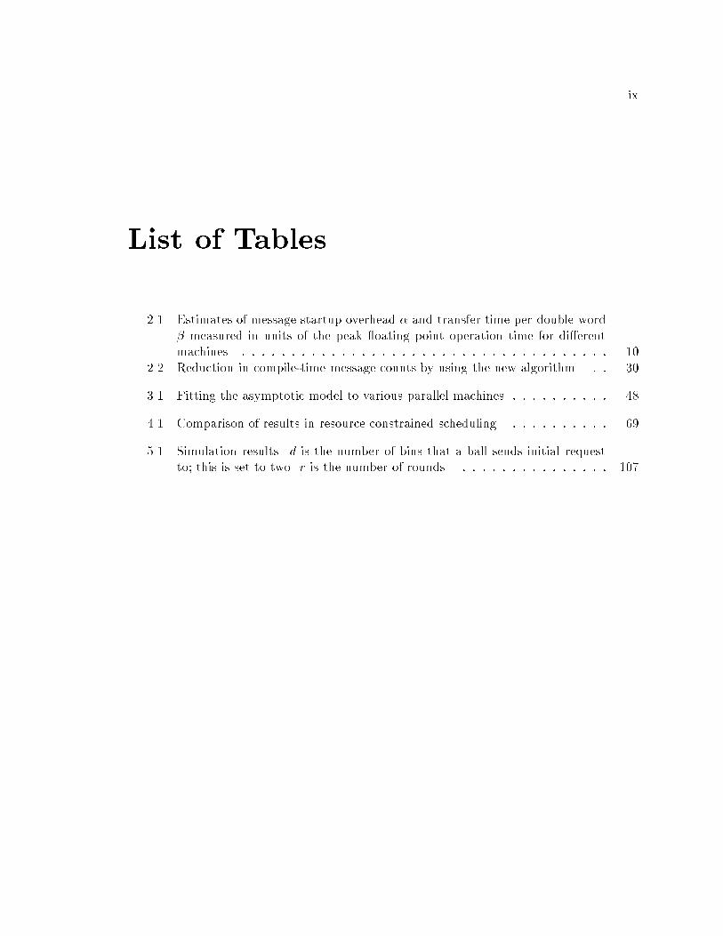
List of Tables ix
1 Introduction 1
1.1 Message scheduling via compiler analysis : : : : : : : : : : : : : : : : : : : : 3
1.2 Scheduling jobs with mixed parallelism : : : : : : : : : : : : : : : : : : : : : 4
1.3 Scheduling resource constrained jobs : : : : : : : : : : : : : : : : : : : : : : 6
1.4 Dynamic scheduling using parallel random allocation : : : : : : : : : : : : 7
2 Message scheduling via compiler analysis 9
2.1 Introduction : : : : : : : : : : : : : : : : : : : : : : : : : : : : : : : : : : : : 9
2.2 Motivating codes : : : : : : : : : : : : : : : : : : : : : : : : : : : : : : : : : 11
2.2.1 Beyond redundancy elimination : : : : : : : : : : : : : : : : : : : : 13
2.2.2 Earliest placement may hurt : : : : : : : : : : : : : : : : : : : : : : 13
2.2.3 Syntax sensitivity : : : : : : : : : : : : : : : : : : : : : : : : : : : : 14
2.3 Network performance : : : : : : : : : : : : : : : : : : : : : : : : : : : : : : 15
2.4 Compiler algorithms : : : : : : : : : : : : : : : : : : : : : : : : : : : : : : : 16
2.4.1 Representation and notation : : : : : : : : : : : : : : : : : : : : : : 18
2.4.2 Identifying the latest position : : : : : : : : : : : : : : : : : : : : : 20
2.4.3 Identifying the earliest position : : : : : : : : : : : : : : : : : : : : 20
2.4.4 Generating candidate positions : : : : : : : : : : : : : : : : : : : : : 24
2.4.5 Subset elimination : : : : : : : : : : : : : : : : : : : : : : : : : : : : 26
2.4.6 Redundancy elimination : : : : : : : : : : : : : : : : : : : : : : : : : 26
2.4.7 Choosing from the candidates : : : : : : : : : : : : : : : : : : : : : : 28
2.4.8 Code generation : : : : : : : : : : : : : : : : : : : : : : : : : : : : : 29
2.5 Performance : : : : : : : : : : : : : : : : : : : : : : : : : : : : : : : : : : : : 30
2.6 Extensions : : : : : : : : : : : : : : : : : : : : : : : : : : : : : : : : : : : : 32
2.6.1 General models : : : : : : : : : : : : : : : : : : : : : : : : : : : : : : 33
2.6.2 Special communication patterns : : : : : : : : : : : : : : : : : : : : 35
2.7 Conclusion : : : : : : : : : : : : : : : : : : : : : : : : : : : : : : : : : : : : 35
vi
3 Scheduling hybrid parallelism 37
3.1 Introduction : : : : : : : : : : : : : : : : : : : : : : : : : : : : : : : : : : : : 37
3.2 Notation : : : : : : : : : : : : : : : : : : : : : : : : : : : : : : : : : : : : : 39
3.3 Switched parallel execution : : : : : : : : : : : : : : : : : : : : : : : : : : : 40
3.3.1 Switching a batch : : : : : : : : : : : : : : : : : : : : : : : : : : : : 42
3.3.2 Precedence graphs : : : : : : : : : : : : : : : : : : : : : : : : : : : : 44
3.4 Modeling and analysis : : : : : : : : : : : : : : : : : : : : : : : : : : : : : : 45
3.4.1 E�ciency of data parallelism : : : : : : : : : : : : : : : : : : : : : : 46
3.4.2 Regular task trees : : : : : : : : : : : : : : : : : : : : : : : : : : : : 48
3.4.3 Analysis : : : : : : : : : : : : : : : : : : : : : : : : : : : : : : : : : : 51
3.4.4 Unbalanced batch problems : : : : : : : : : : : : : : : : : : : : : : : 52
3.4.5 Simulations : : : : : : : : : : : : : : : : : : : : : : : : : : : : : : : : 54
3.5 Experiments : : : : : : : : : : : : : : : : : : : : : : : : : : : : : : : : : : : 58
3.5.1 Software structure : : : : : : : : : : : : : : : : : : : : : : : : : : : : 58
3.5.2 Results : : : : : : : : : : : : : : : : : : : : : : : : : : : : : : : : : : 59
3.6 Related work : : : : : : : : : : : : : : : : : : : : : : : : : : : : : : : : : : : 61
3.7 Discussion : : : : : : : : : : : : : : : : : : : : : : : : : : : : : : : : : : : : : 62
4 Scheduling resource constrained jobs 64
4.1 Introduction : : : : : : : : : : : : : : : : : : : : : : : : : : : : : : : : : : : 64
4.1.1 Model and problem statement : : : : : : : : : : : : : : : : : : : : : : 66
4.1.2 Discussion of results : : : : : : : : : : : : : : : : : : : : : : : : : : : 68
4.2 Motivation : : : : : : : : : : : : : : : : : : : : : : : : : : : : : : : : : : : : 71
4.2.1 Databases : : : : : : : : : : : : : : : : : : : : : : : : : : : : : : : : : 71
4.2.2 Scienti�c applications : : : : : : : : : : : : : : : : : : : : : : : : : : 72
4.2.3 Fidelity : : : : : : : : : : : : : : : : : : : : : : : : : : : : : : : : : : 72
4.3 Makespan lower bound : : : : : : : : : : : : : : : : : : : : : : : : : : : : : 73
4.4 Makespan upper bound : : : : : : : : : : : : : : : : : : : : : : : : : : : : : 75
4.5 Weighted average completion time : : : : : : : : : : : : : : : : : : : : : : : 78
4.5.1 The bicriteria framework : : : : : : : : : : : : : : : : : : : : : : : : 78
4.5.2 DualPack and applications : : : : : : : : : : : : : : : : : : : : : : : 81
4.6 Extensions : : : : : : : : : : : : : : : : : : : : : : : : : : : : : : : : : : : : 84
5 Dynamic scheduling using parallel random allocation 86
5.1 Introduction : : : : : : : : : : : : : : : : : : : : : : : : : : : : : : : : : : : : 86
5.2 Random allocation for dynamic task graphs : : : : : : : : : : : : : : : : : : 87
5.2.1 Models and notation : : : : : : : : : : : : : : : : : : : : : : : : : : : 88
5.2.2 Discussion of results : : : : : : : : : : : : : : : : : : : : : : : : : : : 90
5.2.3 Weighted occupancy : : : : : : : : : : : : : : : : : : : : : : : : : : : 90
5.2.4 Delay sequence : : : : : : : : : : : : : : : : : : : : : : : : : : : : : : 91
5.2.5 Empirical evaluation : : : : : : : : : : : : : : : : : : : : : : : : : : : 94
5.2.6 Discussions : : : : : : : : : : : : : : : : : : : : : : : : : : : : : : : : 96
5.3 Multi-round load balancing protocols : : : : : : : : : : : : : : : : : : : : : 96
5.3.1 The model : : : : : : : : : : : : : : : : : : : : : : : : : : : : : : : : 97
5.3.2 Summary of results : : : : : : : : : : : : : : : : : : : : : : : : : : : : 98
vii
5.3.3 Threshold protocol : : : : : : : : : : : : : : : : : : : : : : : : : : : 98
5.3.4 Other protocols : : : : : : : : : : : : : : : : : : : : : : : : : : : : : : 106
5.3.5 Concluding remarks : : : : : : : : : : : : : : : : : : : : : : : : : : : 107
6 Survey of related work 108
6.1 Communication scheduling : : : : : : : : : : : : : : : : : : : : : : : : : : : 108
6.2 Multiprocessor scheduling : : : : : : : : : : : : : : : : : : : : : : : : : : : : 109
6.3 Minsum metrics : : : : : : : : : : : : : : : : : : : : : : : : : : : : : : : : : : 109
6.4 Resource scheduling : : : : : : : : : : : : : : : : : : : : : : : : : : : : : : : 110
6.5 Distributed load balancing : : : : : : : : : : : : : : : : : : : : : : : : : : : : 111
6.6 Open ends : : : : : : : : : : : : : : : : : : : : : : : : : : : : : : : : : : : : : 111
7 Conclusion 113
Bibliography 115
viii
List of Figures
2.1 The need for combining communication. : : : : : : : : : : : : : : : : : : : : 12
2.2 Earliest placement may lose valuable opportunity for message combining. : 12
2.3 Syntax sensitivity of earliest placement. : : : : : : : : : : : : : : : : : : : : 12
2.4 Bu�er copying and network bandwidth studies on the IBM SP2 and the
Berkeley NOW. : : : : : : : : : : : : : : : : : : : : : : : : : : : : : : : : : : 16
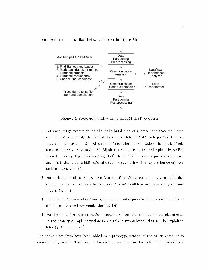
2.5 Prototype modi�cations to the IBM pHPF SPMDizer. : : : : : : : : : : : : 17
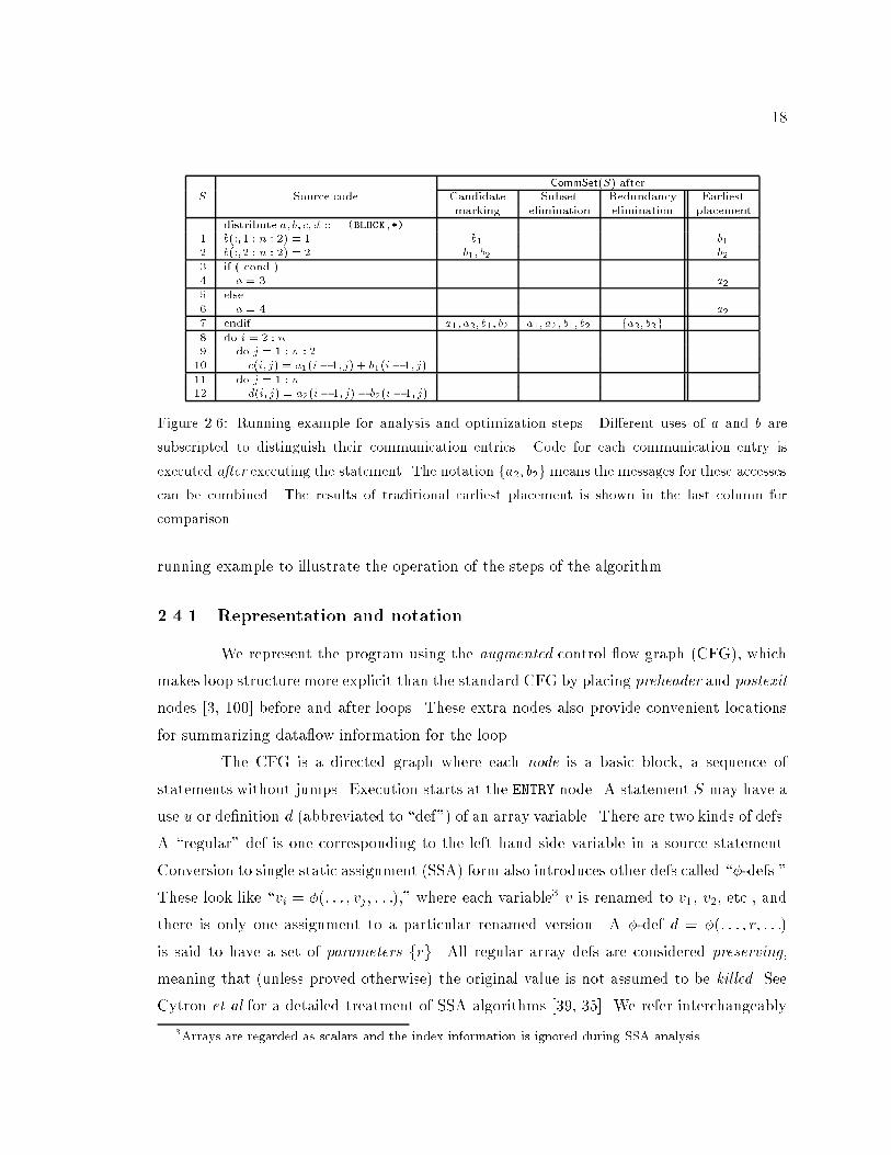
2.6 Running example for analysis and optimization steps. : : : : : : : : : : : : 18
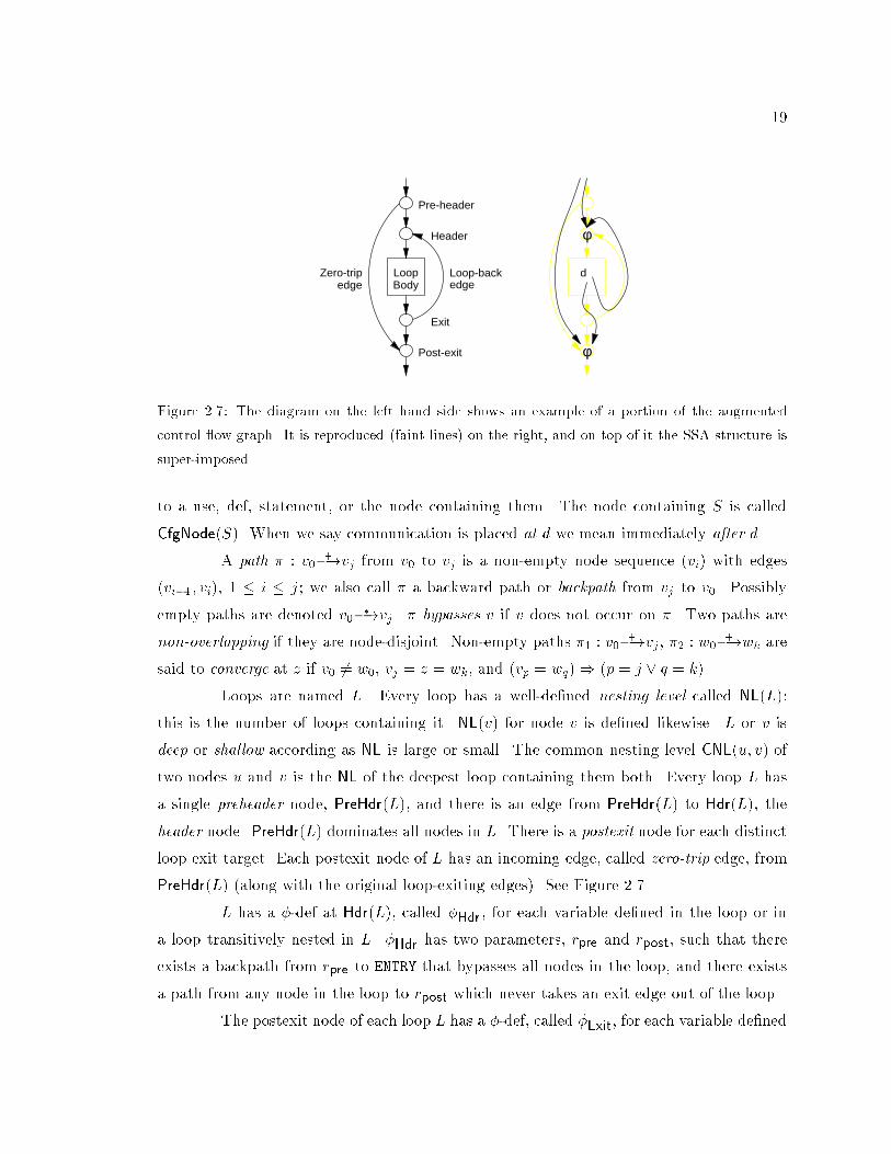
2.7 Augmented single static assignment representation. : : : : : : : : : : : : : : 19
2.8 Pseudocode for locating Earliest and Latest. : : : : : : : : : : : : : : : : : : 21
2.9 Pseudocode for choosing from the candidate positions to place communication. 25
2.10 The candidate communication positions on the dominator tree. : : : : : : : 26
2.11 Performance bene�ts of the new algorithm: normalized running times. : : 31
3.1 An example application with dynamic irregular mixed parallelism. : : : : : 40
3.2 The proposed e�ciency model for data parallelism within a single task. : : 47
3.3 Validation of the asymptotic model using data from ScaLAPACK. : : : : : 49
3.4 Variation of e�ciency with � in sparse Cholesky. : : : : : : : : : : : : : : : 56
3.5 Scalability of sparse Cholesky on four machines using mixed, switched, and
data parallelism. : : : : : : : : : : : : : : : : : : : : : : : : : : : : : : : : : 56
3.6 Plot of e�ciency against problem size for a �xed number of processors. : : : 57
3.7 More e�ciency estimates. : : : : : : : : : : : : : : : : : : : : : : : : : : : : 57
3.8 The software architecture of the dynamic scheduling module in ScaLAPACK. 59
3.9 Performance improvements of switched parallelism over data parallelism on
the Paragon and the SP2. : : : : : : : : : : : : : : : : : : : : : : : : : : : : 60
3.10 Switching and data remapping overheads. : : : : : : : : : : : : : : : : : : : 61
4.1 Illustration of the makespan lower bound. : : : : : : : : : : : : : : : : : : 74
4.2 Existence of bicriteria schedules. : : : : : : : : : : : : : : : : : : : : : : : : 79
5.1 Parallel branch and bound: lower and upper bounds. : : : : : : : : : : : : : 92
5.2 Comparison of speedup between Graham's list schedule and random allocation. 95
5.3 Time break-up of Graham's list schedule and random allocation on the CM5
for the symmetric eigenvalue problem. : : : : : : : : : : : : : : : : : : : : : 95
5.4 A (T; r)-tree with confused balls. : : : : : : : : : : : : : : : : : : : : : : : 104
ix
List of Tables
2.1 Estimates of message startup overhead � and transfer time per double word
� measured in units of the peak oating point operation time for di�erent
machines. : : : : : : : : : : : : : : : : : : : : : : : : : : : : : : : : : : : : : 10
2.2 Reduction in compile-time message counts by using the new algorithm. : : 30
3.1 Fitting the asymptotic model to various parallel machines. : : : : : : : : : : 48
4.1 Comparison of results in resource constrained scheduling. : : : : : : : : : : 69
5.1 Simulation results. d is the number of bins that a ball sends initial request
to; this is set to two. r is the number of rounds. : : : : : : : : : : : : : : : 107
1
Chapter 1
Introduction
Parallelism exists in most forms of computation, and exploiting it is a promising
means to boost the performance of many important scienti�c and commercial applications
beyond peak uniprocessor performance. However, exploiting parallelism is not trivial;
it often requires complete algorithm redesign and implementation for di�erent parallel
machines. It has taken almost a decade to identify a few cost-e�ective parallel architecture
con�gurations, and as a result, system software is only starting to mature and reach a level
of portability and standardization that can motivate application writers to invest in parallel
programming.
This point in time is unique in the development of parallel computing, since some
basic design issues have been resolved, so that one need not chase moving targets any
more, but there is a large scope for algorithm design in systems software. The surviving
architectural choices are clear for the foreseeable future: cost-e�ective parallel machines will
be built from shared memory \symmetric" multiprocessors (SMP's). These will scale up to
a few dozen processors at most. For applications that demand more resources, these SMP's
will be interconnected by a network. Processes on di�erent processors will communicate
by passing messages to each other, either explicitly by subroutine calls, or implicitly, by
accessing remote data and triggering a software abstraction of global memory to issue
messages. In units of CPU cycles, communication overhead is expected to be large. Each
message has some �xed startup overhead time and then some proportional time per byte of
data transfered. It will be the interconnect that will de�ne the character and the price-tag
of the machine; the processors will be commodity.
Apart from interface and portability issues, the challenge for system software, such
2
as compilers, runtime systems, and application libraries, is to export a clean performance
model to the client while adjusting to diverse communication cost parameters and diverse
application behavior in terms of both locality and load balance.
The work in this dissertation is based on the following premises.
� Performance engineering is of paramount importance in parallel computing, because,
\Parallelism is not cheaper or easier, it is faster" [66].
� Scheduling the resources of the multiprocessor (mainly, processors, network, memory,
and IO activity) judiciously between the units of work is essential for achieving high
utilization of the resources. Very few compilers or runtime systems take such a
global view of the scheduling problem yet, and we shall show the bene�ts of doing so
throughout the thesis.
� These resource scheduling algorithms must use simple models of the machine and
the workload, so that the resulting system is performance-portable across diverse
platforms without need for ad-hoc tuning.
The contribution of this thesis is a resource scheduling framework for scienti�c and
commercial applications on scalable multiprocessors, comprising techniques at the compiler,
runtime, and application level.
Despite the attention that the area of resource allocation and job scheduling has
received, many problems in parallel system scheduling lack satisfactory solutions. First,
simple application of existing results to new domains is rarely possible, because the setting
often has crucial details not addressed by classical scheduling literature. Second, the
practical situation is usually complex, and it is hard to abstract a model that is both simple
and faithful to reality. Third, most of the problems are computationally intractable, and
knowledge of complexity and approximations is needed to design algorithms and analyze
them. Finally, practical algorithmics, re ecting both the constraints and simpli�cations
o�ered by practical scenarios, are more important than exploiting powerful but impractical
primitives from theory.
The rest of this chapter summarizes the problems and new solutions described in
the thesis.
3
1.1 Message scheduling via compiler analysis
Parallelism expressed through arrays and loops is very common in scienti�c
numerical applications. Many languages have been designed for expressing array parallelism,
commonly called \data parallelism." The success of data parallelism has reached the stage
where a language standard called High Performance Fortran (HPF) has been de�ned. HPF
extends Fortran with two features: one can refer to regular array sections rather than
individual elements (this extension is also part of Fortran 90 [49]), and give directives to
the compiler to distribute and align arrays on parallel machines. The compiler partitions
computation to match the data distribution and generates communication for remote arrays.
However, compiling HPF code to get performance close to hand-coded message-passing
programs is still a major challenge. On scalable multiprocessors such as the IBM SP2 or
Intel Paragon, a single extra communication step can cost tens of thousands of CPU cycles.
There is a large body of literature on compiler analysis and optimization of
communication generated by loops involving distributed arrays. Initial progress was mostly
restricted to local optimizations at the single loop-nest level; these could not detect and
eliminate communication that is redundant between di�erent loop nests or subroutines. As
a simple example, a single value of a distributed array could be used in several loops after
its de�nition throughout a subroutine; if the array value is unchanged, communication for
the uses should be done once after the de�nition of the value, but without global analysis
it would be done before each loop enclosing an use.
Several factors complicate the situation. The main existing technique to detect
redundancy has been to trace uses of values back to the de�nition and cancel all
communication that is rendered redundant by other communication placed at that point.
This is called earliest placement, and is also good for overlapping communication with
computation. However, this technique places communication for a remote array access at
a place depending only on that access and not others, which may prevent some highly
pro�table optimizations like combining messages from multiple arrays into one. While
message combining amortizes communication overhead, it requires memory copies for
packing and unpacking data. This has to be done carefully so that the communication
bu�ers are smaller than the cache, or the bene�ts of amortizing the �xed overhead of a
message may be canceled by cache miss penalty.
In Chapter 2 we will describe a new compiler algorithm for communication analysis
4
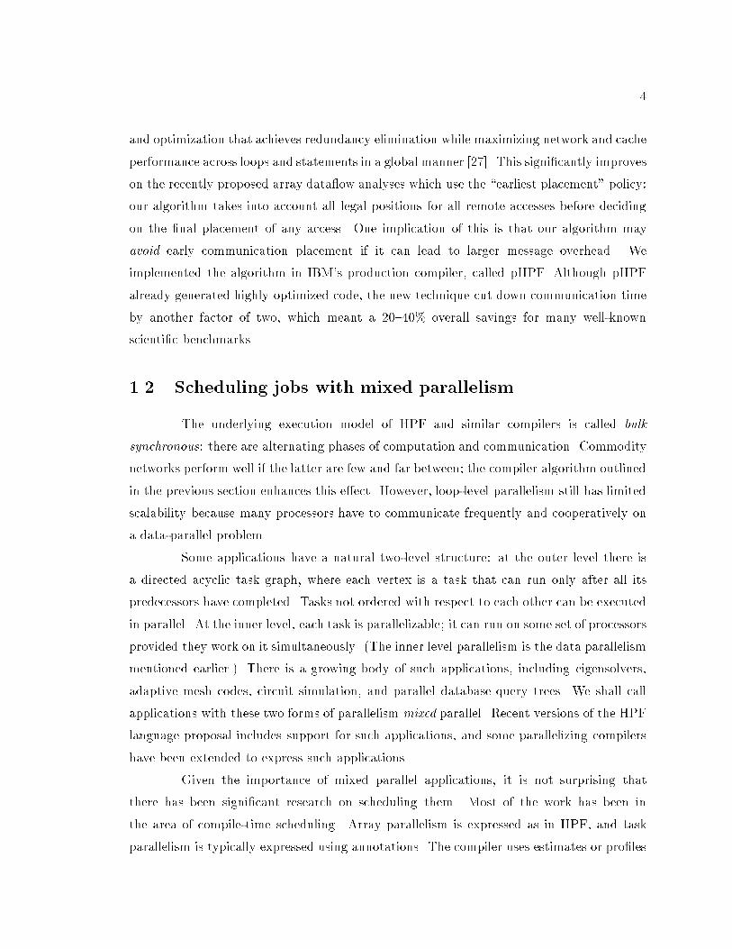
and optimization that achieves redundancy elimination while maximizing network and cache
performance across loops and statements in a global manner [27]. This signi�cantly improves
on the recently proposed array data ow analyses which use the \earliest placement" policy:
our algorithm takes into account all legal positions for all remote accesses before deciding
on the �nal placement of any access. One implication of this is that our algorithm may
avoid early communication placement if it can lead to larger message overhead. We
implemented the algorithm in IBM's production compiler, called pHPF. Although pHPF
already generated highly optimized code, the new technique cut down communication time
by another factor of two, which meant a 20{40% overall savings for many well-known
scienti�c benchmarks.
1.2 Scheduling jobs with mixed parallelism
The underlying execution model of HPF and similar compilers is called bulk
synchronous: there are alternating phases of computation and communication. Commodity
networks perform well if the latter are few and far between; the compiler algorithm outlined
in the previous section enhances this e�ect. However, loop-level parallelism still has limited
scalability because many processors have to communicate frequently and cooperatively on
a data-parallel problem.
Some applications have a natural two-level structure: at the outer level there is
a directed acyclic task graph, where each vertex is a task that can run only after all its
predecessors have completed. Tasks not ordered with respect to each other can be executed
in parallel. At the inner level, each task is parallelizable; it can run on some set of processors
provided they work on it simultaneously. (The inner level parallelism is the data parallelism
mentioned earlier.) There is a growing body of such applications, including eigensolvers,
adaptive mesh codes, circuit simulation, and parallel database query trees. We shall call
applications with these two forms of parallelism mixed parallel. Recent versions of the HPF
language proposal includes support for such applications, and some parallelizing compilers
have been extended to express such applications.
Given the importance of mixed parallel applications, it is not surprising that
there has been signi�cant research on scheduling them. Most of the work has been in
the area of compile-time scheduling. Array parallelism is expressed as in HPF, and task
parallelism is typically expressed using annotations. The compiler uses estimates or pro�les
5
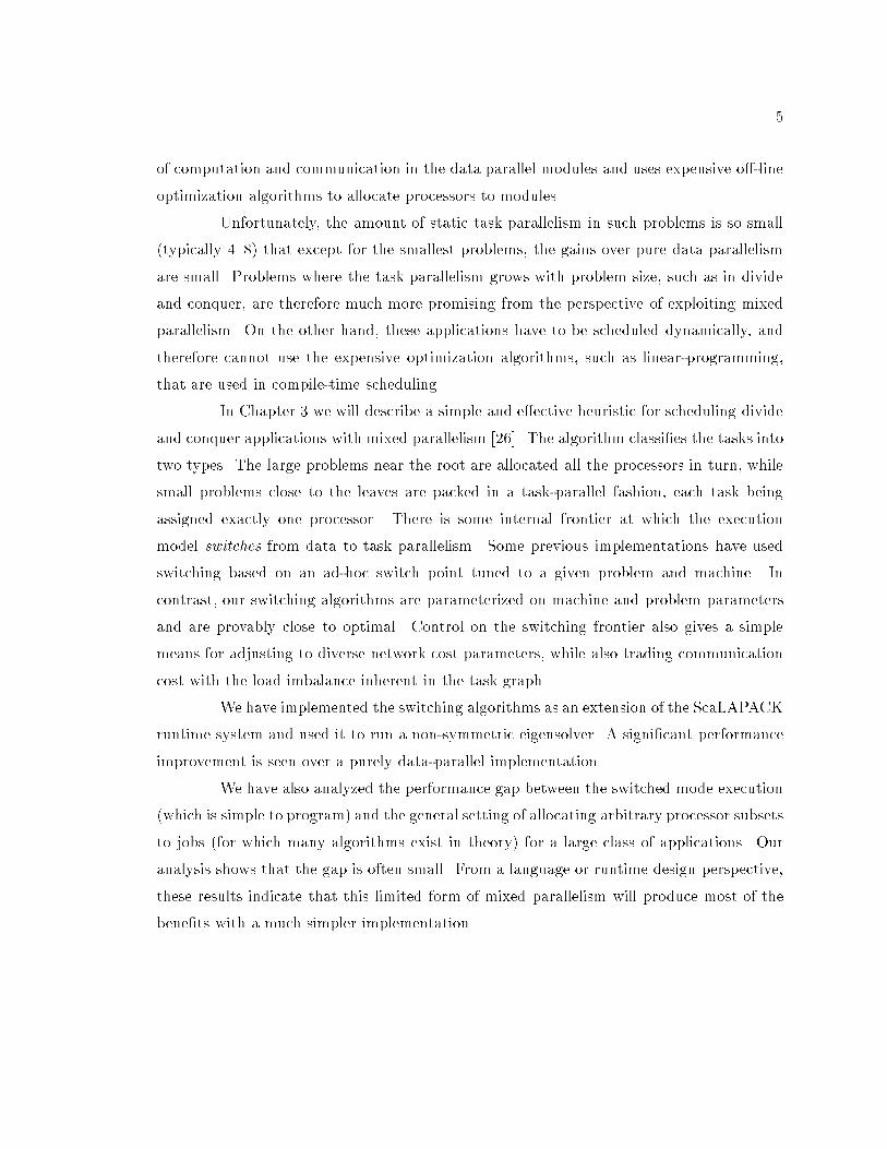
of computation and communication in the data parallel modules and uses expensive o�-line
optimization algorithms to allocate processors to modules.
Unfortunately, the amount of static task parallelism in such problems is so small
(typically 4{8) that except for the smallest problems, the gains over pure data parallelism
are small. Problems where the task parallelism grows with problem size, such as in divide
and conquer, are therefore much more promising from the perspective of exploiting mixed
parallelism. On the other hand, these applications have to be scheduled dynamically, and
therefore cannot use the expensive optimization algorithms, such as linear-programming,
that are used in compile-time scheduling.
In Chapter 3 we will describe a simple and e�ective heuristic for scheduling divide
and conquer applications with mixed parallelism [26]. The algorithm classi�es the tasks into
two types. The large problems near the root are allocated all the processors in turn, while
small problems close to the leaves are packed in a task-parallel fashion, each task being
assigned exactly one processor. There is some internal frontier at which the execution
model switches from data to task parallelism. Some previous implementations have used
switching based on an ad-hoc switch point tuned to a given problem and machine. In
contrast, our switching algorithms are parameterized on machine and problem parameters
and are provably close to optimal. Control on the switching frontier also gives a simple
means for adjusting to diverse network cost parameters, while also trading communication
cost with the load imbalance inherent in the task graph.
We have implemented the switching algorithms as an extension of the ScaLAPACK
runtime system and used it to run a non-symmetric eigensolver. A signi�cant performance
improvement is seen over a purely data-parallel implementation.
We have also analyzed the performance gap between the switched mode execution
(which is simple to program) and the general setting of allocating arbitrary processor subsets
to jobs (for which many algorithms exist in theory) for a large class of applications. Our
analysis shows that the gap is often small. From a language or runtime design perspective,
these results indicate that this limited form of mixed parallelism will produce most of the
bene�ts with a much simpler implementation.
6
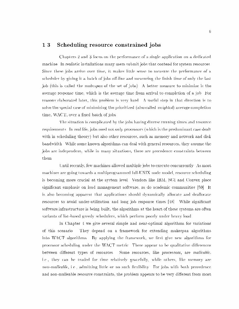
1.3 Scheduling resource constrained jobs
Chapters 2 and 3 focus on the performance of a single application on a dedicated
machine. In realistic installations many users submit jobs that contend for system resources.
Since these jobs arrive over time, it makes little sense to measure the performance of a
scheduler by giving it a batch of jobs o�-line and measuring the �nish time of only the last
job (this is called the makespan of the set of jobs). A better measure to minimize is the
average response time, which is the average time from arrival to completion of a job. For
reasons elaborated later, this problem is very hard. A useful step in that direction is to
solve the special case of minimizing the prioritized (also called weighted) average completion
time, WACT, over a �xed batch of jobs.
The situation is complicated by the jobs having diverse running times and resource
requirements. In real life, jobs need not only processors (which is the predominant case dealt
with in scheduling theory) but also other resources, such as memory and network and disk
bandwidth. While some known algorithms can deal with general resources, they assume the
jobs are independent, while in many situations, there are precedence constraints between
them.
Until recently, few machines allowed multiple jobs to execute concurrently. As most
machines are going towards a multiprogrammed full-UNIX node model, resource scheduling
is becoming more crucial at the system level. Vendors like IBM, SGI and Convex place
signi�cant emphasis on load management software, as do academic communities [50]. It
is also becoming apparent that applications should dynamically allocate and deallocate
resources to avoid under-utilization and long job response times [48]. While signi�cant
software infrastructure is being built, the algorithms at the heart of these systems are often
variants of list-based greedy schedulers, which perform poorly under heavy load.
In Chapter 4 we give several simple and near-optimal algorithms for variations
of this scenario. They depend on a framework for extending makespan algorithms
into WACT algorithms. By applying the framework, we �rst give new algorithms for
processor scheduling under the WACT metric. There appear to be qualitative di�erences
between di�erent types of resources. Some resources, like processors, are malleable,
i.e., they can be traded for time relatively gracefully, while others, like memory are
non-malleable, i.e., admitting little or no such exibility. For jobs with both precedence
and non-malleable resource constraints, the problem appears to be very di�erent from most
7
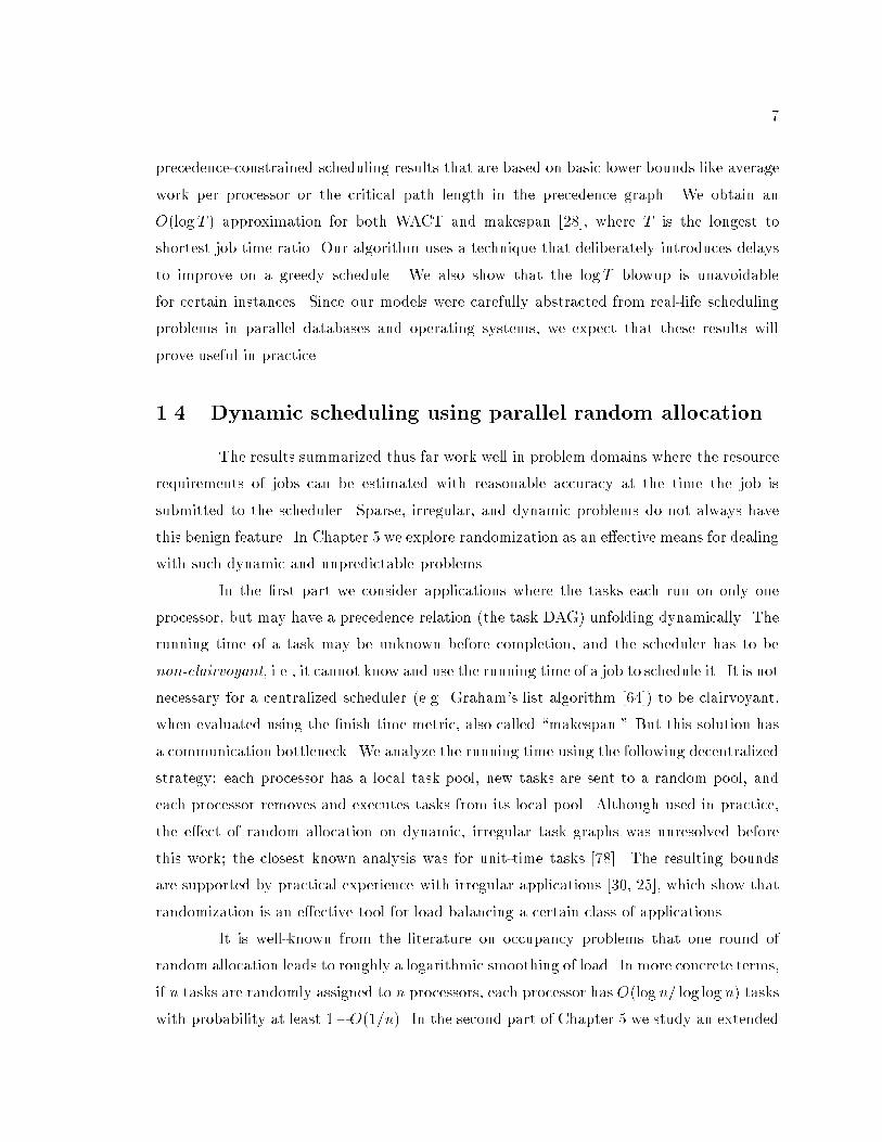
precedence-constrained scheduling results that are based on basic lower bounds like average
work per processor or the critical path length in the precedence graph. We obtain an
O(logT ) approximation for both WACT and makespan [28], where T is the longest to
shortest job time ratio. Our algorithm uses a technique that deliberately introduces delays
to improve on a greedy schedule. We also show that the logT blowup is unavoidable
for certain instances. Since our models were carefully abstracted from real-life scheduling
problems in parallel databases and operating systems, we expect that these results will
prove useful in practice.
1.4 Dynamic scheduling using parallel random allocation
The results summarized thus far work well in problem domains where the resource
requirements of jobs can be estimated with reasonable accuracy at the time the job is
submitted to the scheduler. Sparse, irregular, and dynamic problems do not always have
this benign feature. In Chapter 5 we explore randomization as an e�ective means for dealing
with such dynamic and unpredictable problems.
In the �rst part we consider applications where the tasks each run on only one
processor, but may have a precedence relation (the task DAG) unfolding dynamically. The
running time of a task may be unknown before completion, and the scheduler has to be
non-clairvoyant, i.e., it cannot know and use the running time of a job to schedule it. It is not
necessary for a centralized scheduler (e.g. Graham's list algorithm [64]) to be clairvoyant,
when evaluated using the �nish time metric, also called \makespan." But this solution has
a communication bottleneck. We analyze the running time using the following decentralized
strategy: each processor has a local task pool, new tasks are sent to a random pool, and
each processor removes and executes tasks from its local pool. Although used in practice,
the e�ect of random allocation on dynamic, irregular task graphs was unresolved before
this work; the closest known analysis was for unit-time tasks [78]. The resulting bounds
are supported by practical experience with irregular applications [30, 25], which show that
randomization is an e�ective tool for load balancing a certain class of applications.
It is well-known from the literature on occupancy problems that one round of
random allocation leads to roughly a logarithmic smoothing of load. In more concrete terms,
if n tasks are randomly assigned to n processors, each processor has O(logn= log log n) tasks
with probability at least 1�O(1=n). In the second part of Chapter 5 we study an extended
8
model of random allocation, where assignment of tasks to processors are made in multiple
rounds so as to further smooth down the load imbalance to sub-logarithmic amounts. In
addition to the task scheduling application, this setting can be motivated by the problem of
allocating �le blocks in distributed \serverless" �le systems like xFS [6]. In this setting there
are n client workstations whose local disks comprise the �le system, which can be abstracted
as n servers. As clients write �les, new disk blocks must be allocated in a decentralized
way without overloading any particular server. There is a trade-o� between the cost of
communication to obtain more global information and the cost of load imbalance owing to
imperfect knowledge. At one extreme, one can send each new block to a random server; at
the other, one can get optimal load balance by maintaining exact global load information.
We give a precise characterization of this trade-o� [1]. Initial simulation results agree with
theoretical predictions.
Extensive work has been done on all the problems studied. In Chapter 6 we will
present a survey and classi�cation of known results based on job and machine models.
Finally, in Chapter 7 we will summarize the thesis and suggest directions for future work.
9
Chapter 2
Message scheduling via compiler
analysis
2.1 Introduction
Distributed memory architectures provide a cost-e�ective method for building
scalable parallel computers. However, the absence of a global address space and the resulting
need for explicit message passing makes these machines di�cult to program. This has
motivated the design of languages like High Performance Fortran (HPF) [55], which allow
the programmer to write sequential or shared-memory parallel programs that are annotated
with directives specifying data decomposition. The compilers for these languages are
responsible for partitioning the computation and generating the communication necessary
to fetch values of non-local data referenced by a processor [72, 123, 20, 5, 21, 68].
Accessing remote data is usually orders of magnitude slower than accessing
local data, for the following reasons. It is getting increasingly cost-e�ective to build
multiprocessors from commodity hardware components and system software. Most current
generation CPU's are well beyond the 100MFLOPS mark, and are consistently out-pacing
network performance. Most vendors support UNIX-like environments on each processor, in
particular with multiprogramming and virtual memory. This means that low-overhead
message passing implementations like Active Messages [115], which work best with
gang-scheduled time slicing, user-level access to the network interface, and register-based
data transfer, are not the best choice. As a result, communication startup overheads tend
10
Machine NW software � �
Paragon NX 7:8� 103
9
Cray T3D BLT 2:7� 104
9
CM5+VU CMMD 1:4� 104
103
IBM SP1 MPL 2:8� 104
50
IBM SP2 MPL 1:2� 104
60
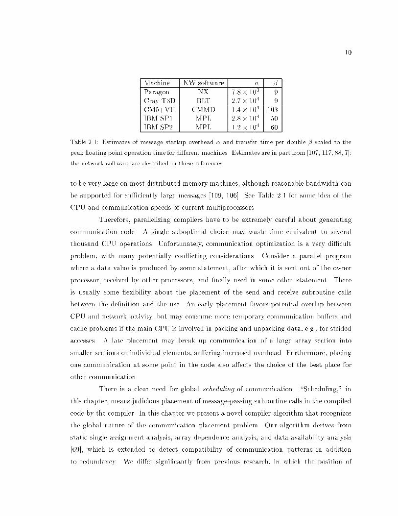
Table 2.1: Estimates of message startup overhead � and transfer time per double � scaled to the
peak oating point operation time for di�erent machines. Estimates are in part from [107, 117, 88, 7];
the network software are described in these references.
to be very large on most distributed memory machines, although reasonable bandwidth can
be supported for su�ciently large messages [109, 106]. See Table 2.1 for some idea of the
CPU and communication speeds of current multiprocessors.
Therefore, parallelizing compilers have to be extremely careful about generating
communication code. A single suboptimal choice may waste time equivalent to several
thousand CPU operations. Unfortunately, communication optimization is a very di�cult
problem, with many potentially con icting considerations. Consider a parallel program
where a data value is produced by some statement, after which it is sent out of the owner
processor, received by other processors, and �nally used in some other statement. There
is usually some exibility about the placement of the send and receive subroutine calls
between the de�nition and the use. An early placement favors potential overlap between
CPU and network activity, but may consume more temporary communication bu�ers and
cache problems if the main CPU is involved in packing and unpacking data, e.g., for strided
accesses. A late placement may break up communication of a large array section into
smaller sections or individual elements, su�ering increased overhead. Furthermore, placing
one communication at some point in the code also a�ects the choice of the best place for
other communication.
There is a clear need for global scheduling of communication. \Scheduling," in
this chapter, means judicious placement of message-passing subroutine calls in the compiled
code by the compiler. In this chapter we present a novel compiler algorithm that recognizes
the global nature of the communication placement problem. Our algorithm derives from
static single assignment analysis, array dependence analysis, and data availability analysis
[69], which is extended to detect compatibility of communication patterns in addition
to redundancy. We di�er signi�cantly from previous research, in which the position of
11
communication code for each remote access is decided independent of other remote accesses;
instead, we determine the positions in an interdependent and global manner. The algorithm
achieves both redundancy elimination and message combining globally, and is able to reduce
the number of messages to an extent that is not achievable with any previous approach.
Our algorithm has been implemented in the IBM pHPF prototype compiler [68].
We report results from a preliminary study of some well-known HPF programs. The
performance gains are impressive. Reduction in static message count can be up to a factor
of almost nine. Time spent in communication is reduced in many cases by a factor of two or
more. We believe that these are also the �rst results from any implementation of redundant
message elimination across di�erent loop nests, and add signi�cant experimental experience
to research on communication optimization.
2.2 Motivating codes
We will use a few code fragments to show the importance of recognizing the global
nature of the message placement problem. We are interested in the communication patterns
and the exibility in message placement revealed by data dependence analysis, not the
particulars of the applications.
In the code fragments that we present, we will elide actual operations and show
each right hand side (RHS) as a list of variables accessed. Frequently we deal with Fortran 90
(F90) style shift operations that involve nearest-neighbor communication; we show this
pictorially using arrows. For simplicity, the combinable messages in our examples have
identical patterns on the processor template; in practice, combining is feasible when one
pattern is a subset of another.
Speci�cally, we demonstrate the following.
� Redundancy elimination is useful, but often not enough to reduce the number of
messages. Reducing message count is crucial for our target architectures, especially
for synchronous and collective communication.
� The traditional mechanisms of redundancy elimination can sometimes prevent the
compiler from generating the best communication code.
� The well-known redundancy elimination technique of earliest communication place-
ment is sensitive to minor syntactic di�erences in the high-level source, and may
12
Timestep loop:
glast(:; :) = g(1; : : :)
for i = 2 to nx� 1
� � � = g(i; :; :)" #!
� � � = sum(g(i;ny; :));sum(g(i;ny� 1; :));sum(g(i;0; :));sum(g(i; 1; :))
� � � = glast(:; :)" #!
� � � = sum(glast(ny; :));sum(glast(ny� 1; :));sum(glast(0; :));sum(glast(1; :))
glast(:; :) = g(i; :; :)
g(i; :; :) = � � �
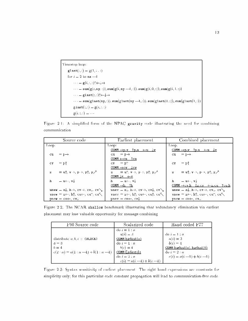
Figure 2.1: A simpli�ed form of the NPAC gravity code illustrating the need for combining
communication.
Source code Earliest placement Combined placement
Loop:
cu = p!
cv = p"
z = u", v!, p!, p", p%
h = u , v#
unew = z#, h!, cv!, cv#, cv&
vnew = z , h", cu , cu", cu-
pnew = cu , cv#
Loop:
COMM!p,v "p,u u #vcu = p!
COMM cu "cucv = p"
COMM!cv #cv
z = u", v!, p!, p", p%COMM #z z
h = u , v#
COMM!h "hunew = z#, h!, cv!, cv#, cv&
vnew = z , h", cu , cu", cu-
pnew = cu , cv#
Loop:
COMM!p,v "p,u u #vcu = p!
cv = p"
z = u", v!, p!, p", p%
h = u , v#
COMM!cv,h #z,cv z,cu "cu,h
unew = z#, h!, cv!, cv#, cv&
vnew = z , h", cu , cu", cu-
pnew = cu , cv#
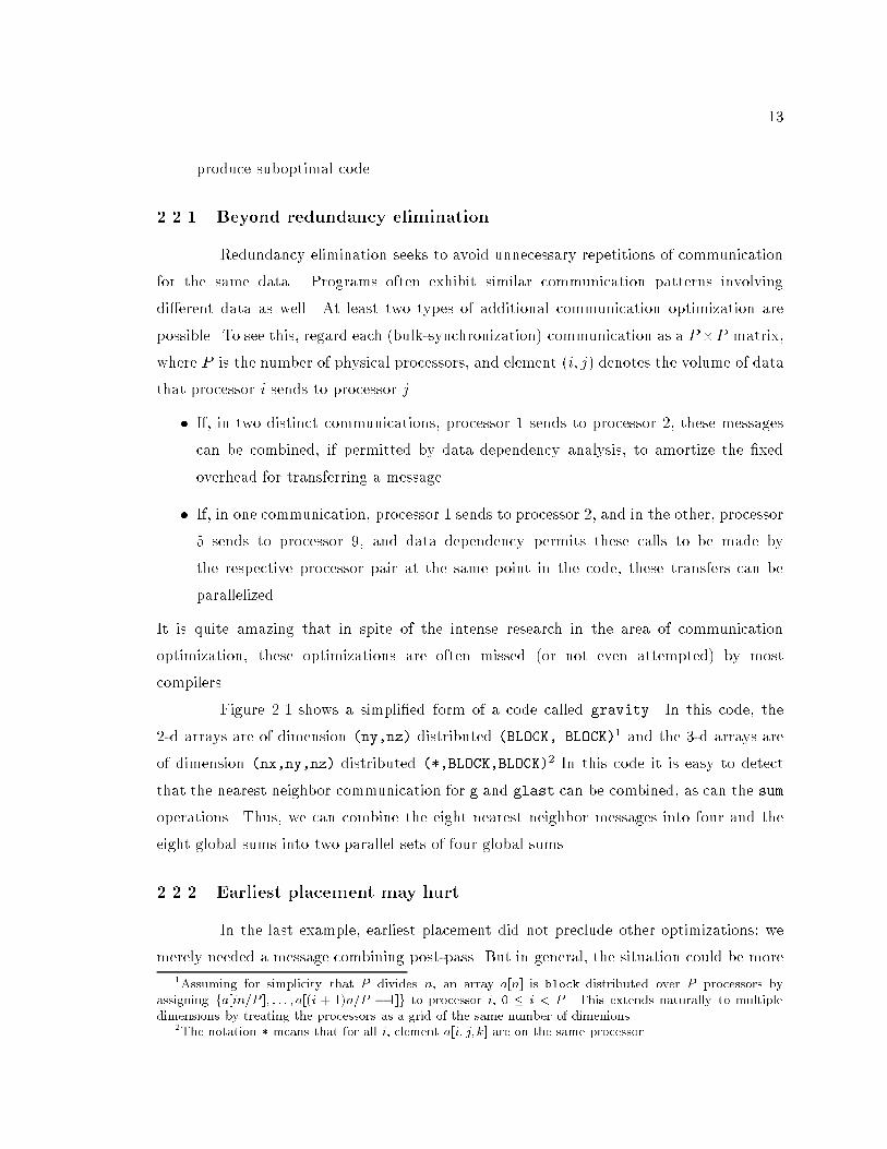
Figure 2.2: The NCAR shallow benchmark illustrating that redundancy elimination via earliest
placement may lose valuable opportunity for message combining.
F90 Source code Scalarized code Hand coded F77
distribute a; b; c :: (BLOCK)
a = 3b = 4
c(2 : n) = a(1 : n� 1) + b(1 : n� 1)
do i = 1 : na(i) = 3
COMM Earliest(a)
do i = 1 : nb(i) = 4
COMM Earliest(b)
do i = 2 : nc(i) = a(i� 1) + b(i� 1)
do i = 1 : n
a(i) = 3
b(i) = 4COMM Earliest(a);Earliest(b)
do i = 2 : n
c(i) = a(i� 1) + b(i� 1)
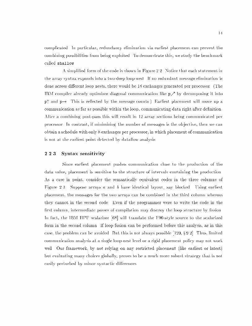
Figure 2.3: Syntax sensitivity of earliest placement. The right hand expressions are constants for
simplicity only; for this particular code constant propagation will lead to communication-free code.
13
produce suboptimal code.
2.2.1 Beyond redundancy elimination
Redundancy elimination seeks to avoid unnecessary repetitions of communication
for the same data. Programs often exhibit similar communication patterns involving
di�erent data as well. At least two types of additional communication optimization are
possible. To see this, regard each (bulk-synchronization) communication as a P �P matrix,
where P is the number of physical processors, and element (i; j) denotes the volume of data
that processor i sends to processor j.
� If, in two distinct communications, processor 1 sends to processor 2, these messages
can be combined, if permitted by data dependency analysis, to amortize the �xed
overhead for transferring a message.
� If, in one communication, processor 1 sends to processor 2, and in the other, processor
5 sends to processor 9, and data dependency permits these calls to be made by
the respective processor pair at the same point in the code, these transfers can be
parallelized.
It is quite amazing that in spite of the intense research in the area of communication
optimization, these optimizations are often missed (or not even attempted) by most
compilers.
Figure 2.1 shows a simpli�ed form of a code called gravity. In this code, the
2-d arrays are of dimension (ny,nz) distributed (BLOCK, BLOCK)1 and the 3-d arrays are
of dimension (nx,ny,nz) distributed (*,BLOCK,BLOCK)2 In this code it is easy to detect
that the nearest neighbor communication for g and glast can be combined, as can the sum
operations. Thus, we can combine the eight nearest neighbor messages into four and the
eight global sums into two parallel sets of four global sums.
2.2.2 Earliest placement may hurt
In the last example, earliest placement did not preclude other optimizations; we
merely needed a message combining post-pass. But in general, the situation could be more
1Assuming for simplicity that P divides n, an array a[n] is block distributed over P processors by
assigning fa[in=P ]; : : : ; a[(i + 1)n=P � 1]g to processor i, 0 � i < P . This extends naturally to multiple
dimensions by treating the processors as a grid of the same number of dimenions.2The notation * means that for all i, element a[i; j; k] are on the same processor.
14
complicated. In particular, redundancy elimination via earliest placement can prevent the
combining possibilities from being exploited. To demonstrate this, we study the benchmark
called shallow.
A simpli�ed form of the code is shown in Figure 2.2. Notice that each statement in
the array syntax expands into a two-deep loop-nest. If no redundant message elimination is
done across di�erent loop nests, there would be 18 exchanges generated per processor. (The
IBM compiler already optimizes diagonal communication like p% by decomposing it into
p" and p!. This is re ected by the message counts.) Earliest placement will move up a
communication as far as possible within the loop, communicating data right after de�nition.
After a combining post-pass this will result in 12 array sections being communicated per
processor. In contrast, if minimizing the number of messages is the objective, then we can
obtain a schedule with only 8 exchanges per processor, in which placement of communication
is not at the earliest point detected by data ow analysis.
2.2.3 Syntax sensitivity
Since earliest placement pushes communication close to the production of the
data value, placement is sensitive to the structure of intervals containing the production.
As a case in point, consider the semantically equivalent codes in the three columns of
Figure 2.3. Suppose arrays a and b have identical layout, say blocked. Using earliest
placement, the messages for the two arrays can be combined in the third column whereas
they cannot in the second code. Even if the programmer were to write the code in the
�rst column, intermediate passes of compilation may destroy the loop structure by �ssion.
In fact, the IBM HPF scalarizer [68] will translate the F90-style source to the scalarized
form in the second column. If loop fusion can be performed before this analysis, as in this
case, the problem can be avoided. But this is not always possible [120, x 9.2]. Thus, limitedcommunication analysis at a single loop-nest level or a rigid placement policy may not work
well. Our framework, by not relying on any restricted placement (like earliest or latest)
but evaluating many choices globally, proves to be a much more robust strategy that is not
easily perturbed by minor syntactic di�erences.
15
2.3 Network performance
By pro�ling our target networks, we justify the need for global message scheduling
and identify simplifying assumptions that can be made about the optimization problem.
We pick two platforms: the IBM SP2 with a custom network, and a network of Sparc
workstations (NOW) connected by a commodity network (Myrinet). The SP2 uses IBM's
message passing library MPL; the NOW uses MPICH, a portable implementation of the MPI
standard from Argonne National Labs. Details of the networks can be found in [109, 106, 79].
We want to measure the bene�ts of large messages, while estimating the local block copy
(bcopy) cost to collect many small messages into a large one. Figure 2.4 shows the pro�ling
code and results.
We will be mostly interested in e�ective bandwidth since the HPF runtime does
bulk transfer as the common case. For �ne-grained communication, there is a distinction
between CPU overhead per message, which cannot be overlapped with computation, and
network latency, which can. In the bulk-synchronous execution model that HPF compiles
down to, the bene�ts of overlap are very small. Kennedy et al estimate this to be typically
5{9% for 2-d stencil problems of size 256� 256 on a 16-processor iPSC/860, in the context
of the Fortran-D execution model and runtime system [81].
The top curve shows the bandwidth of local block copy (bcopy) as a function of
bu�er size. The bottom curve plots network bandwidth as a function of message length,
based on the time that the receiver waits for completion.
The top curve shows that as long as the message bu�ers �t in cache, we can
ignore the overhead of bcopy. Fortunately, for both machines, most of the message startup
amortization bene�ts occur at message sizes much smaller than the cache limit; given typical
cache sizes, we believe this is a fairly general feature.
On the other hand, for messages much larger than cache, it may be important to
suppress combining communication from non-contiguous array sections. E.g., for the SP2,
the bandwidth of copying bu�ers larger than the cache is barely twice the message-passing
bandwidth beyond cache size.
If there is a network co-processor or DMA, it is possible for the sender to quickly
inject the message and the receiver to retrieve it more slowly. The middle curve shows
bandwidth computed using the time the sender takes to inject the message. While the
injection bandwidth is much lower than bcopy, it is larger than receive bandwidth for
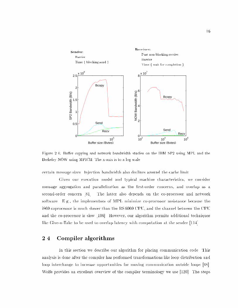
16
Sender:
Barrier
Time f blocking send g
Receiver:
Post non-blocking receive
Barrier
Time f wait for completion g
105
0
0.5
1
1.5
2
2.5x 10
8
Buffer size (Bytes)
SP
2 B
andw
idth
(B
/s)
Recv
Send
Bcopy
102
104
106
0
2
4
6
8x 10
7
Buffer size (Bytes)
NO
W B
andw
idth
(B
/s)
RecvSend
Bcopy
Figure 2.4: Bu�er copying and network bandwidth studies on the IBM SP2 using MPL and the
Berkeley NOW using MPICH. The x-axis is to a log scale.
certain message sizes. Injection bandwidth also declines around the cache limit.
Given our execution model and typical machine characteristics, we consider
message aggregation and parallelization as the �rst-order concerns, and overlap as a
second-order concern [81]. The latter also depends on the co-processor and network
software. E.g., the implementors of MPL minimize co-processor assistance because the
i860 coprocessor is much slower than the RS 6000 CPU, and the channel between the CPU
and the co-processor is slow [106]. However, our algorithm permits additional techniques
like Give-n-Take to be used to overlap latency with computation at the sender [114].
2.4 Compiler algorithms
In this section we describe our algorithm for placing communication code. This
analysis is done after the compiler has performed transformations like loop distribution and
loop interchange to increase opportunities for moving communication outside loops [68].
Wolfe provides an excellent overview of the compiler terminology we use [120]. The steps
17
of our algorithm are described below and shown in Figure 2.5.
for hand compilation
Modified pHPF SPMDizer
Dataflow/Dependence
Analyzer
LoopTransformer
2. Mark candidate statements1. Find Earliest and Latest
3. Eliminate subsets4. Eliminate redundancy5. Choose final candidate
Trace dump to lst file
Communication
Partitioning
Analysis
CommunicationCode Generation
DataPartitioning
Postprocessing
Preprocessing
Data
Figure 2.5: Prototype modi�cations to the IBM pHPF SPMDizer.
1. For each array expression on the right hand side of a statement that may need
communication, identify the earliest (x2.4.3) and latest (x2.4.2) safe position to place
that communication. One of our key innovations is to exploit the static single
assignment (SSA) information [39, 35] already computed in an earlier phase by pHPF,
re�ned by array dependence-testing [121]. In contrast, previous proposals for such
analysis typically use a bidirectional data ow approach with array section descriptors
and/or bit-vectors [69].
2. For each non-local reference, identify a set of candidate positions, any one of which
can be potentially chosen as the �nal point to emit a call to a message-passing runtime
routine (x2.4.4).
3. Perform the \array-section" analog of common subexpression elimination: detect and
eliminate subsumed communication (x2.4.6).
4. For the remaining communication, choose one from the set of candidate placements.
In the prototype implementation we do this in two substeps that will be explained
later (x2.4.5 and x2.4.7).
The above algorithms have been added to a prototype version of the pHPF compiler as
shown in Figure 2.5. Throughout this section, we will use the code in Figure 2.6 as a
18
CommSet(S) afterS Source code Candidate Subset Redundancy Earliest
marking elimination elimination placement
distribute a; b; c; d :: (BLOCK,*)
1 b(:;1 : n : 2) = 1 b1 b1
2 b(:;2 : n : 2) = 2 b1; b2 b2
3 if ( cond )4 a = 3 a2
5 else6 a = 4 a2
7 endif a1; a2; b1; b2 a1; a2; b1; b2 fa2; b2g8 do i = 2 : n9 do j = 1 : n : 2
10 c(i; j) = a1(i� 1; j) + b1(i� 1; j)
11 do j = 1 : n12 d(i; j) = a2(i� 1; j)� b2(i� 1; j)
Figure 2.6: Running example for analysis and optimization steps. Di�erent uses of a and b are
subscripted to distinguish their communication entries. Code for each communication entry is
executed after executing the statement. The notation fa2; b2g means the messages for these accesses
can be combined. The results of traditional earliest placement is shown in the last column for
comparison.
running example to illustrate the operation of the steps of the algorithm.
2.4.1 Representation and notation
We represent the program using the augmented control ow graph (CFG), which
makes loop structure more explicit than the standard CFG by placing preheader and postexit
nodes [3, 100] before and after loops. These extra nodes also provide convenient locations
for summarizing data ow information for the loop.
The CFG is a directed graph where each node is a basic block, a sequence of
statements without jumps. Execution starts at the ENTRY node. A statement S may have a
use u or de�nition d (abbreviated to \def") of an array variable. There are two kinds of defs.
A \regular" def is one corresponding to the left hand side variable in a source statement.
Conversion to single static assignment (SSA) form also introduces other defs called \�-defs."
These look like \vi = �(: : : ; vj ; : : :)," where each variable3 v is renamed to v1, v2, etc., and
there is only one assignment to a particular renamed version. A �-def d = �(: : : ; r; : : :)
is said to have a set of parameters frg. All regular array defs are considered preserving,
meaning that (unless proved otherwise) the original value is not assumed to be killed. See
Cytron et al for a detailed treatment of SSA algorithms [39, 35]. We refer interchangeably
3Arrays are regarded as scalars and the index information is ignored during SSA analysis.
19
Post-exit
Exit
edgeLoop-back
Pre-header
Header
dBodyLoop
edgeZero-trip
φ
φ
Figure 2.7: The diagram on the left hand side shows an example of a portion of the augmented
control ow graph. It is reproduced (faint lines) on the right, and on top of it the SSA structure is
super-imposed.
to a use, def, statement, or the node containing them. The node containing S is called
CfgNode(S). When we say communication is placed at d we mean immediately after d.
A path � : v0+�!vj from v0 to vj is a non-empty node sequence (vi) with edges
(vi�1; vi), 1 � i � j; we also call � a backward path or backpath from vj to v0. Possibly
empty paths are denoted v0��!vj . � bypasses v if v does not occur on �. Two paths are
non-overlapping if they are node-disjoint. Non-empty paths �1 : v0+�!vj , �2 : w0
+�!wk are
said to converge at z if v0 6= w0, vj = z = wk, and (vp = wq)) (p = j _ q = k).
Loops are named L. Every loop has a well-de�ned nesting level called NL(L):
this is the number of loops containing it. NL(v) for node v is de�ned likewise. L or v is
deep or shallow according as NL is large or small. The common nesting level CNL(u; v) of
two nodes u and v is the NL of the deepest loop containing them both. Every loop L has
a single preheader node, PreHdr(L), and there is an edge from PreHdr(L) to Hdr(L), the
header node. PreHdr(L) dominates all nodes in L. There is a postexit node for each distinct
loop exit target. Each postexit node of L has an incoming edge, called zero-trip edge, from
PreHdr(L) (along with the original loop-exiting edges). See Figure 2.7.
L has a �-def at Hdr(L), called �Hdr , for each variable de�ned in the loop or in
a loop transitively nested in L. �Hdr has two parameters, rpre and rpost, such that there
exists a backpath from rpre to ENTRY that bypasses all nodes in the loop, and there exists
a path from any node in the loop to rpost which never takes an exit edge out of the loop.
The postexit node of each loop L has a �-def, called �Exit, for each variable de�ned
20
in the loop or in a loop transitively nested in it. Because of �Exit, a de�nition d can reach
a use u only through a de�nition d0 at a level CNL(d; u). d0 can possibly be d only if
CNL(d; u) = NL(d); otherwise, d0 is a �-def at a level CNL(d; u).
2.4.2 Identifying the latest position
We describe how the compiler �nds Latest(u), the latest point to place communi-
cation for u, which is also placed in as shallow a loop level as possible, so that messages are
maximally vectorized. This follows from standard communication analysis: communication
is placed just before the outermost loop in which there is no true dependence on u, and is
placed just before the statement containing u if no such loop exists [123, 72, 68].
Given a use u, let d range over the reaching regular defs of u. (Reaching
defs are de�ned in Cytron et al [39, 35].) Consider some d. Observe that it is never
necessary to place communication for u deeper than at CNL(d; u). Given d and u, we
can compute all possible direction vectors (each is a CNL(d; u)-dimensional vector) [120].
These vectors are used in the routine IsArrayDep, shown in Figure 2.8(d) on page 21.
Let DepLevel(d; u) = maxf` : IsArrayDep(d; u; `)g, the deepest level at which there is a
loop-carried dependency between u and d.
Because of the dependency at level DepLevel(d; u), communication for u cannot
be moved outside loop level DepLevel(d; u). The overall communication level for use u,
denoted CommLevel(u), is set to maxdfDepLevel(d; u)g. Finally, to place communication,
we check CommLevel(u): if CommLevel(u) = NL(u), communication is placed immediately
before the statement containing u4; if CommLevel(u) < NL(u), communication is placed
in the loop preheader of the loop at level (CommLevel(u) + 1) that contains u. Note that
CommLevel(u) > NL(u) is not possible, and that by construction Latest(u) dominates u.
2.4.3 Identifying the earliest position
We now describe how to compute Earliest(u) for use u. Typically, data ow analysis
with array sections marks a set of nodes as \earliest", such that a copy of the communication
code has to be placed at all these points. This is acceptable if each array section is
communicated using a separate call to the communication library, but for our purposes,
it greatly complicates code generation. In di�erent control ow paths, communication for u
4In this case no vectorization has been possible.
21
a. Earliest(u)
For each def d of use u in depth-�rst preorder traversal:
If Test(d; u) then return d.
b. Test(d; u)
If d is a �-def, say d = �(: : : ; ri; : : :)
For each �-parameter rivisit[�] = 0, visit[d] = 1
Let ci = Rcount(Reaching(ri); u;CNL(d; u); visit)
If two or more ci's are positive
Return TRUE
else (d is a regular def)
If IsArrayDep(d; u;CNL(d; u))
Return TRUE.
c. Rcount(d; u; l;visit)
If d is a �-def, say d = �(: : : ; ri; : : :)
If visit[d] return 0
visit[d] = 1
Return
PiRcount(Reaching(ri); u; l; visit)
else (d is a regular def)
If IsArrayDep(d; u; l)
Return 1
else if d is a preserving def
Return Rcount(Reaching(d); u; l;visit)
else return 0.
d. IsArrayDep(d; u; `)
If d is the pseudo-def at ENTRY then return TRUE
If ` > CNL(d; u) then return FALSE
If 9 direction vector ~v = (v1; : : : ; vCNL(d;u)) such that
� vi = 0, for i 2 f1; : : : ; `� 1g, and� v` � 0
then return TRUE
else return FALSE
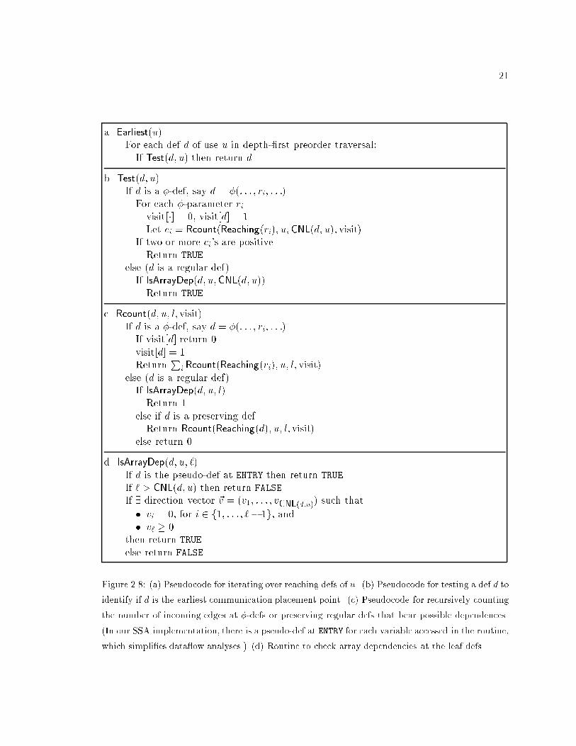
Figure 2.8: (a) Pseudocode for iterating over reaching defs of u. (b) Pseudocode for testing a def d to
identify if d is the earliest communication placement point. (c) Pseudocode for recursively counting
the number of incoming edges at �-defs or preserving regular defs that bear possible dependences.
(In our SSA implementation, there is a pseudo-def at ENTRY for each variable accessed in the routine,
which simpli�es data ow analyses.) (d) Routine to check array dependencies at the leaf defs.
22
may be combined with di�erent references, making it impossible to generate a single version
of the original computation containing u. The resulting code expansion can be enormous.
Moreover, each message will need to have a descriptor for their contents, because, depending
on the control path taken at runtime, the arrays packaged into a message may be di�erent.
Therefore, we restrict our search to the single earliest position that dominates the
use. Our experience with benchmarks, albeit limited, suggests that further sophistication
is often unnecessary. The pseudocode for computing Earliest(u) for a use u is shown in
Figure 2.8(a{d). Earliest goes through defs reaching u in a certain order, Testing each in
turn and returning with the �rst success. Test calls Rcount to �nd out if communication
can be pushed beyond the candidate def d, or that the def represents a merge of at least
two values and is hence a critical point to place communication. Rcount recurses through
reaching defs of d, calling IsArrayDep at the leaves of the recursion, which are regular defs.
Claim 2.4.1 Earliest(u) returns the earliest single dominating communication point d1 for
use u.
In Figure 2.6, Earliest(a1) = Earliest(a2) = 7. Traditional array data ow analysis, which
does not insist on dominating defs [69], would lead to Earliest0(a1) = Earliest0(a2) = f4; 6g.In both cases, a2 subsumes a1. We prove Claim 2.4.1 using the following three lemmas.
Lemma 2.4.2 d1 dominates u.
Proof. (By contradiction.) We assume d1 is not the pseudo-def at ENTRY, since the latter
dominates all nodes in the CFG. Let `1 = NL(d1), and L1 be the loop containing d1. Note
that `1 � NL(u) because Earliest will never ag a d1 with NL(d1) > NL(u). Assume d1 does
not dominate u. Then there exist two or more paths: one from ENTRY to u that bypasses
d1, and another from d1 to u. If NL(u) = NL(d1), these two paths imply that there exists
a �-def at level `1 with (at least) two parameters, r1 and r2, such that there exist two
non-overlapping backpaths: one from r1 to d1, and the other from r2 to the pseudo-def
at ENTRY that bypasses d1. (Because of the zero-trip edges, we can ignore other loops
nested in L1.). That there is such a �-def at level `1 still holds if NL(u) > NL(d1), because
the preheader node of each loop containing u dominates u, and the two (or more) paths
converge at the preheader node which is at level `1, at the latest. Test is called on at least
one of these �-defs, say p, before d1 during the traversal of Earliest(u), starting from u.
23
During execution of Test(p; u), Rcount gets called on defs Reaching(r1) and Reaching(r2),
with nesting level CNL(p; u) = `1. The call at Reaching(r1) returns a positive number,
because some recursive call inspects d1. Similarly the call at Reaching(r2) also returns a
positive number, because some recursive call inspects ENTRY. Since at least two invocations
of Rcount return a positive numbers, the �-def, not d1, will be returned as Earliest(u) if d1
does not dominate u, a contradiction.
Lemma 2.4.3 Let n3 be any proper dominator-tree ancestor of d1. Then there exists a
regular def d2 such that IsArrayDep(d2; u;CNL(d1; u)) returns TRUE, and there also exists a
path d2��!d1
+�!u that bypasses n3.
Proof. If d1 is the pseudo-def at ENTRY, there is nothing to prove. Also, if d1 is a regular
def, IsArrayDep(d1; u;CNL(d1; u)) must hold for d1 to be returned as Earliest(u), in which
case d1 serves as the de�nition d2 in the statement of the lemma. Therefore, we can assume
d1 is a �-def.
By design, Test(d1) returned TRUE because at least two Rcount calls on the
�-parameters of d1 returned positive counts. But because of the visit[ ] array, no def is
accounted more than once. Therefore the two positive counts can be attributed to two
node-disjoint backpaths to two distinct regular defs (one of which could be ENTRY). At
most one of these paths contain n3. Let d2 be some regular def on the other path such that
IsArrayDep(d2; u;CNL(d1; u)) = TRUE. Then there is a d2+�!u path bypassing n3.
Lemma 2.4.4 There is no regular def d4 along a path d1+�!d4
+�!u such that
IsArrayDep(d4; u;CNL(d4; u)) returns TRUE, and there is a path from d4 to u that bypasses d1.
That is, it su�ces to place communication at d1.
Proof. (By contradiction.) Assume there exists such a d4. According to SSA construction,
two cases can occur: either (1) d4, as well as d1, dominates u, or (2) d4 has a path, bypassing
d1, from it to u through one or more �-defs that dominate u.
Case 1. If d4 dominates u, d4 cannot also dominate d1. Otherwise, there exists a path
from ENTRY to d4 to u that bypasses d1 (second condition in the lemma), in which case d1
cannot dominate u, contradicting Lemma 2.4.2. Therefore, d1 dominates d4 (note that if
both d4 and d1 dominate u, one of them must dominate the other), which in turn dominates
u. Thus Test(d4; u) is called before Test(d1; u) by Earliest(u). Test(d4; u) = TRUE because
IsArrayDep(d4; u;CNL(d4; u)) = TRUE, so d4 will get returned as Earliest(u); a contradiction.
24
Case 2. In the second case, d1 dominates the �-defs. If not, then d1 would not dominate u
either, (contrary to Lemma 2.4.2) because there is a path d4+�!� +�!u avoiding d1. Hence,
these �-defs are dominated by d1 and are visited before d1 by Earliest(u). It follows, from a
similar argument in the proof of Lemma 2.4.2, that these two paths converge at some node
at level CNL(d4; u), creating a �-def at level CNL(d4; u). This �-node has (at least) two
parameters, r1 and r2, such that there exist two non-overlapping paths: one from d4 to r1,
and the other from d1 to r2. When applied to r1, Rcount returns positive, possibly because
of d4, which satis�es IsArrayDep(d4; u;CNL(d4; u)). When applied to r2, Rcount returns
positive, possibly because of the pseudo-def at ENTRY. Since (at least) two parameters
return positive, the �-def, not d1, is returned by Earliest(u), another contradiction.
Proof of Claim 2.4.1. Observe that only a node that dominates u can serve as a single
communication point for u. Lemma 2.4.2 says that d1 = Earliest(u) dominates u. Consider
all dominator-tree ancestors of u. From this set, Lemma 2.4.3 rules out all nodes that strictly
dominate d1 as unsafe. Finally, Lemma 2.4.4 implies that d1 is a safe communication point
for u.
2.4.4 Generating candidate positions
Since any safe position to insert a single copy of communication for use u must
dominate u, the set of candidate positions has a very simple characterization in terms of
the following claims. We omit the proofs; see Figure 2.10 for the justi�cation.
Claim 2.4.5 Starting at the basic block containing Latest(u), denoted c(Latest(u)), if we
follow parent links in the dominator tree of the CFG, we will reach the basic block containing
Earliest(u).
Claim 2.4.6 The statements marked in the basic blocks encountered during the dominator
tree traversal from c(Latest(u)) up to c(Earliest(u)) are exactly those that are single candidate
positions for communication placement for use u.
Our algorithm for �nding candidate placements of communication is thus ex-
tremely simple, and shown in Figure 2.9(e). In our example (Figure 2.6), statements 3,
4, 5, and 6 are not candidates for placing communication for accesses b1 and b2 because
they do not dominate those uses.
25
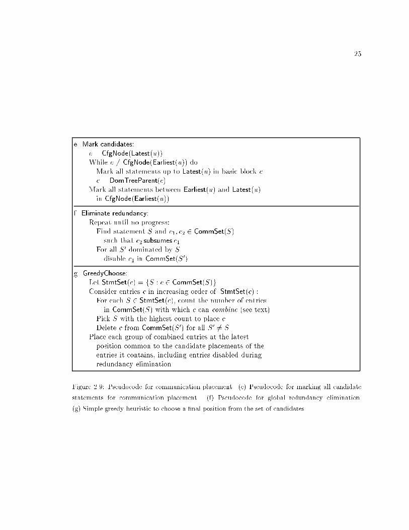
e. Mark candidates:
c = CfgNode(Latest(u))
While c 6= CfgNode(Earliest(u)) do
Mark all statements up to Latest(u) in basic block c
c = DomTreeParent(c)
Mark all statements between Earliest(u) and Latest(u)
in CfgNode(Earliest(u)).
f. Eliminate redundancy:
Repeat until no progress:
Find statement S and c1; c2 2 CommSet(S)
such that c2 subsumes c1For all S0 dominated by S
disable c1 in CommSet(S0)
g. GreedyChoose:
Let StmtSet(c) = fS : c 2 CommSet(S)gConsider entries c in increasing order of jStmtSet(c)j:For each S 2 StmtSet(c), count the number of entries
in CommSet(S) with which c can combine (see text)
Pick S with the highest count to place c
Delete c from CommSet(S0) for all S0 6= S
Place each group of combined entries at the latest
position common to the candidate placements of the
entries it contains, including entries disabled during
redundancy elimination.
Figure 2.9: Pseudocode for communication placement. (e) Pseudocode for marking all candidate
statements for communication placement. (f) Pseudocode for global redundancy elimination.
(g) Simple greedy heuristic to choose a �nal position from the set of candidates.
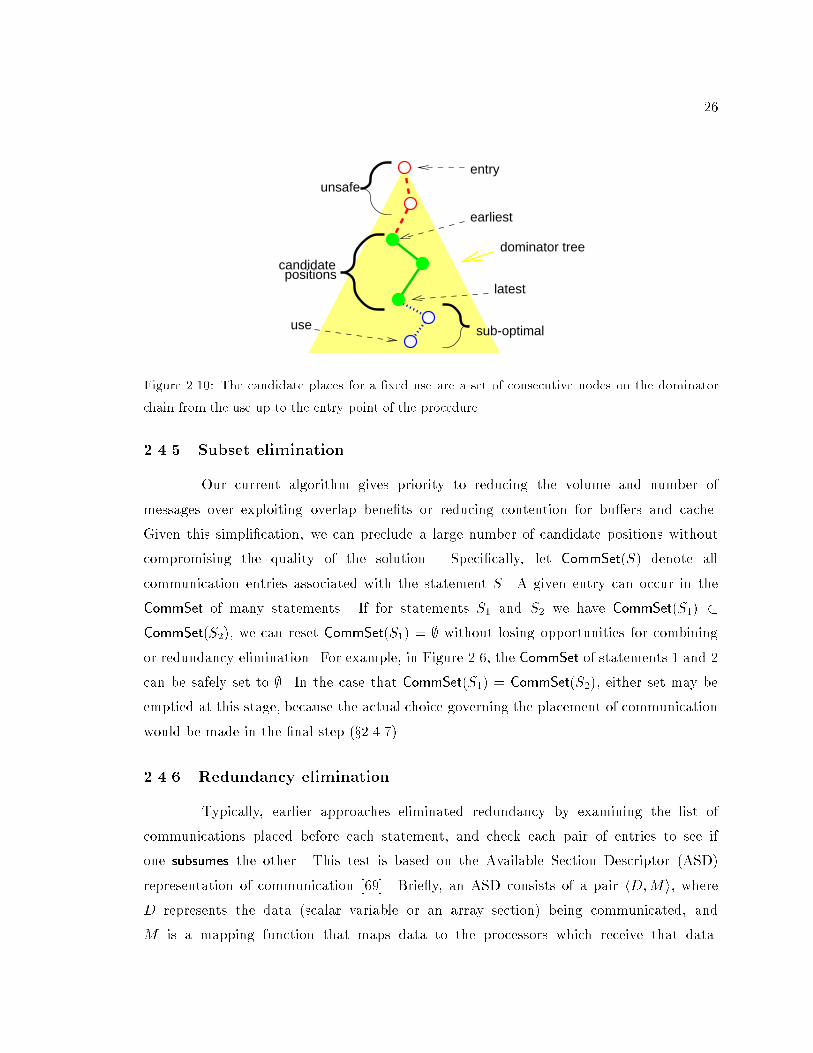
26
positionscandidate
earliest
use sub-optimal
unsafe
latest
dominator tree
entry
Figure 2.10: The candidate places for a �xed use are a set of consecutive nodes on the dominator
chain from the use up to the entry point of the procedure.
2.4.5 Subset elimination
Our current algorithm gives priority to reducing the volume and number of
messages over exploiting overlap bene�ts or reducing contention for bu�ers and cache.
Given this simpli�cation, we can preclude a large number of candidate positions without
compromising the quality of the solution. Speci�cally, let CommSet(S) denote all
communication entries associated with the statement S. A given entry can occur in the
CommSet of many statements. If for statements S1 and S2 we have CommSet(S1) �CommSet(S2), we can reset CommSet(S1) = ; without losing opportunities for combining
or redundancy elimination. For example, in Figure 2.6, the CommSet of statements 1 and 2
can be safely set to ;. In the case that CommSet(S1) = CommSet(S2), either set may be
emptied at this stage, because the actual choice governing the placement of communication
would be made in the �nal step (x2.4.7).
2.4.6 Redundancy elimination
Typically, earlier approaches eliminated redundancy by examining the list of
communications placed before each statement, and check each pair of entries to see if
one subsumes the other. This test is based on the Available Section Descriptor (ASD)
representation of communication [69]. Brie y, an ASD consists of a pair hD;Mi, whereD represents the data (scalar variable or an array section) being communicated, and
M is a mapping function that maps data to the processors which receive that data.
27
A communication hD1;M1i is made redundant by another communication hD2;M2i if
D1 � D2, and M1(D1) �M2(D1).
In our case, since there can be many entries for a reference, we have to
propagate the redundancy information globally. The pseudocode for eliminating redundant
communication in the context of our current framework is shown in Figure 2.9(f). The
modi�cation is that in each step examining a statement S, the subsumed communication
entry is cleared not only from CommSet(S) but from all statements S0 such that S dominates
S0. (The dominance ordering prevents a cycle of deletions.) We iterate over statements
and communication pairs until no more elimination occurs.
Claim 2.4.7 The subset and redundancy elimination steps are safe, i.e., the remaining
communication entries are su�cient.
Proof. Subset elimination in an arbitrary order is clearly safe because � is transitive.
The only concern is that when we throw away all copies of an entry because it was found
subsumed at one place, its copy may earlier have subsumed some other communication at
another place.
Let entries e1; e2 2 CommSet(S1) and e2; e3 2 CommSet(S2). Since e2 is in both,
assume w.l.o.g. that S1 dominates S2. We say that ej is redundant if ASD(ej) � ASD(ei),
for some statement S, and ei; ej 2 CommSet(S).
The possible mishap sequence is that we �nd ASD(e3) � ASD(e2) at S2, delete e3
from all S, �nd ASD(e2) � ASD(e1) at S1, and delete e2 from all S, including S1 and S2. If
the remaining entry e1 does not remain available at S2, it must be due to a def d of some
data in ASD(e3) between S1 and S2. But in that case, since d 2 ASD(e2), e2 could not have
occurred at both S1 and S2 in the �rst place.
One implication of the above ordering of eliminations is noteworthy. Consider
our running example (Figure 2.6), speci�cally the communication due to the uses b1
and b2 (ASD(b1) � ASD(b2), since b1 represents b[2 : n; 1 : n : 2] and b1 represents
b[2 : n; 1 : n]). Since Earliest(b1) = 1 6= Earliest(b2) = 2, an initial test of redundancy
based on earliest placement, followed by candidate marking and subset elimination will not
catch the redundancy. Thus, by choosing a placement for b1 later than Earliest(b1), we are
able to eliminate the communication for b1 completely. In contrast, the solution proposed
in [69] would move each communication to the earliest point, and reduce the communication
28
for b2 to ASD(b2)�ASD(b1), while the communication for b1 would remain unchanged. The
solution obtained with our current method is superior because it reduces the communication
startup overhead, and it makes code generation much simpler.
2.4.7 Choosing from the candidates
At this stage we can still have a communication entry c in multiple CommSet's,
and we have to arbitrate in favor of one. The goal is to minimize the total communication
cost. In the common message cost model using �xed overhead per message and bandwidth,
minimizing the cost is NP-hard (also see x2.6). In practice, simple greedy heuristics work
quite well; see Figure 2.9(g). It is similar to Click's global code motion heuristic [36]:
consider the most constrained communication entry next, and put it where it is compatible
in communication pattern (as shown by the test below) with the largest number of other
candidate communication. A more re�ned heuristic would use estimates of message sizes
and consider the communication cost if the current entry were combined with a given set
of entries.
The entries in the CommSet of each statement can now be partitioned into groups,
each group consisting of one or more entries which will be combined into a single aggregate
communication operation. Any exibility still available in placing this aggregate can be
used to push this communication later, if reducing contention for bu�ers and cache is
more important than overlap bene�ts (as is folk truism for the SP2), or push it earlier if
the situation were reversed. Our algorithm places communication for each group at the
latest position common to the possible placements of each entry in that group (including
positions disabled during the previous step for redundancy elimination). Deferring the
placement decision until this �nal step enables our algorithm to take advantage of any
possible placement that leads to redundancy elimination or combining bene�ts, without
the drawback of unnecessary movement of communication that uses up more resources or
degrades performance.
Criteria for communication compatibility. While in principle, code for arbitrary
communications can be combined into code for a single communication operation, we are
interested in combining messages only when the startup overheads associated with all but
one of them can be eliminated, leading to improved performance. Hence, we view two
communications as compatible for combining if the associated sender-receiver relationships
29
are identical or one is a subset of the other.
Thus, communications for hD1;M1i and hD2;M2i are combined only if M1 =M2
or M1 � M2. The combined communication is given by hD1 [D2;M2i. In order to ensure
better performance and for simplicity of code generation, we impose the following additional
constraints on combining.
� The combined data size of D1 [D2 must be below a threshold (based on our study
reported in x2.3, currently set to 20 KB for SP2), beyond which combining messages
leads to diminishing returns or even worse performance. When data sizes are unknown,
the compiler uses rules of thumb like assuming that nearest-neighbor communication
(NNC) and reductions (where volume of data communicated is signi�cantly lower than
that involved in computation) are operating within the range suitable for combining.
� The size of D1 [ D2, as approximated by a single section descriptor (array sections
are not closed under the union operation), should not exceed the combined size of D1
and D2 by more than a small constant. This descriptor for D1[D2 refers to identical
sections of di�erent arrays if D1 and D2 correspond to di�erent arrays, and to a single
array otherwise.
The check for M1 � M2 is done in the virtual processor space of template positions,
as described in [69]. However, we have incorporated extensions to check for equality of
mappings in physical processor space for nearest-neighbor communication and for mappings
to a constant processor position [69].
2.4.8 Code generation
As shown in Figure 2.5, the step after communication analysis and optimization
is to insert communication code in the form of subroutine calls to the pHPF runtime
library routines, which in turn invoke MPL/MPI. The runtime library provides a high-level
interface through which the compiler speci�es the data being communicated in the form of
array sections, and the runtime system takes care of packing and unpacking of data. For
NNC, data is received in overlap regions [123] surrounding the local portion of the arrays.
For other kinds of communication involving arrays, data is received into a bu�er that is
allocated dynamically, and the array reference that led to this communication is replaced
by a reference to the bu�er.
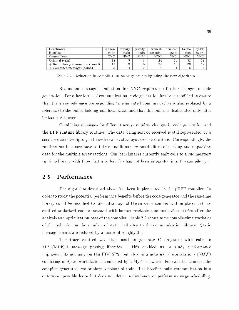
30
Benchmark shallow gravity gravity trimesh trimesh hyd o hyd oRoutine main main main normdot gauss ux hydro
Comm Type NNC NNC SUM NNC NNC NNC NNC
Original (orig) 18 8 8 24 13 52 12+ Redundancy elimination (nored) 12 8 8 24 13 30 12+ Combined messages (comb) 8 4 2 4 4 6 6
Table 2.2: Reduction in compile-time message counts by using the new algorithm.
Redundant message elimination for NNC requires no further change to code
generation. For other forms of communication, code generation has been modi�ed to ensure
that the array reference corresponding to eliminated communication is also replaced by a
reference to the bu�er holding non-local data, and that this bu�er is deallocated only after
its last use is over.
Combining messages for di�erent arrays requires changes in code generation and
the HPF runtime library routines. The data being sent or received is still represented by a
single section descriptor, but now has a list of arrays associated with it. Correspondingly, the
runtime routines now have to take on additional responsibilities of packing and unpacking
data for the multiple array sections. Our benchmarks currently emit calls to a rudimentary
runtime library with these features, but this has not been integrated into the compiler yet.
2.5 Performance
The algorithm described above has been implemented in the pHPF compiler. In
order to study the potential performance bene�ts before the code generator and the run-time
library could be modi�ed to take advantage of the superior communication placement, we
emitted scalarized code annotated with human readable communication entries after the
analysis and optimization pass of the compiler. Table 2.2 shows some compile-time statistics
of the reduction in the number of static call sites to the communication library. Static
message counts are reduced by a factor of roughly 2{9.
The trace emitted was then used to generate C programs with calls to
MPL/MPICH message passing libraries. This enabled us to study performance
improvements not only on the IBM SP2, but also on a network of workstations (NOW)
consisting of Sparc workstations connected by a Myrinet switch. For each benchmark, the
compiler generated two or three versions of code. The baseline pulls communication into
outermost possible loops but does not detect redundancy or perform message scheduling.
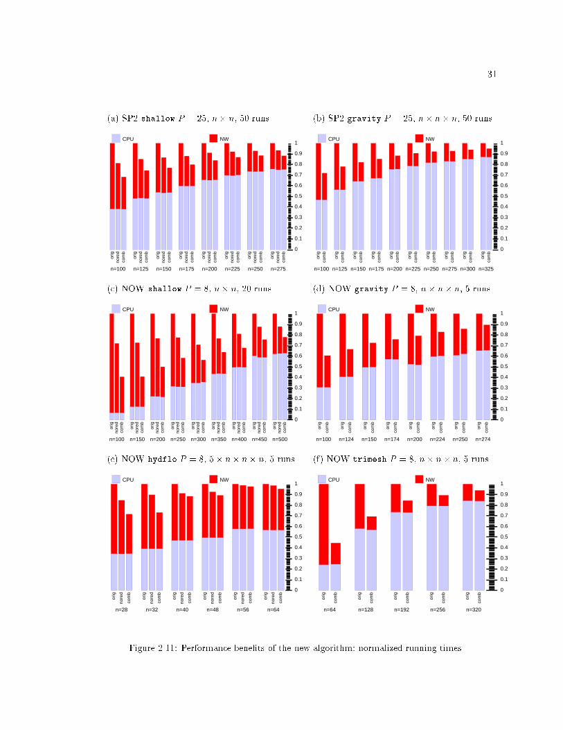
31
(a) SP2 shallow P = 25, n� n, 50 runs
CPU NW
0
0.1
0.2
0.3
0.4
0.5
0.6
0.7
0.8
0.9
1
orig
nor
ed c
omb
n=100
orig
nor
ed c
omb
n=125
orig
nor
ed c
omb
n=150
orig
nor
ed c
omb
n=175
orig
nor
ed c
omb
n=200
orig
nor
ed c
omb
n=225
orig
nor
ed c
omb
n=250 o
rig n
ored
com
b
n=275
(b) SP2 gravity P = 25, n� n � n, 50 runs
CPU NW
0
0.1
0.2
0.3
0.4
0.5
0.6
0.7
0.8
0.9
1
orig
com
b
n=100
orig
com
b
n=125
orig
com
b
n=150
orig
com
b
n=175
orig
com
b
n=200
orig
com
b
n=225
orig
com
b
n=250
orig
com
b
n=275
orig
com
b
n=300
orig
com
b
n=325
(c) NOW shallow P = 8, n� n, 20 runs
CPU NW
0
0.1
0.2
0.3
0.4
0.5
0.6
0.7
0.8
0.9
1
orig
nor
ed c
omb
n=100
orig
nor
ed c
omb
n=150
orig
nor
ed c
omb
n=200
orig
nor
ed c
omb
n=250
orig
nor
ed c
omb
n=300
orig
nor
ed c
omb
n=350
orig
nor
ed c
omb
n=400
orig
nor
ed c
omb
n=450
orig
nor
ed c
omb
n=500
(d) NOW gravity P = 8, n� n� n, 5 runs
CPU NW
0
0.1
0.2
0.3
0.4
0.5
0.6
0.7
0.8
0.9
1 o
rig
com
b
n=100
orig
com
b
n=124
orig
com
b
n=150
orig
com
b
n=174
orig
com
b
n=200 o
rig
com
b n=224
orig
com
b
n=250
orig
com
b
n=274
(e) NOW hydflo P = 8, 5� n� n� n, 5 runs
CPU NW
0
0.1
0.2
0.3
0.4
0.5
0.6
0.7
0.8
0.9
1
orig
nor
ed
com
b
n=28
orig
nor
ed
com
b
n=32
orig
nor
ed
com
b
n=40
orig
nor
ed
com
b
n=48
orig
nor
ed
com
b
n=56
orig
nor
ed
com
b
n=64
(f) NOW trimesh P = 8, n� n � n, 5 runs
CPU NW
0
0.1
0.2
0.3
0.4
0.5
0.6
0.7
0.8
0.9
1
orig
com
b
n=64
orig
com
b
n=128
orig
com
b
n=192
orig
com
b
n=256
orig
com
b
n=320
Figure 2.11: Performance bene�ts of the new algorithm: normalized running times.
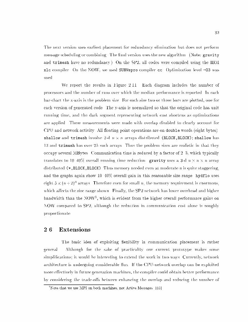
32
The next version uses earliest placement for redundancy elimination but does not perform
message scheduling or combining. The �nal version uses the new algorithm. (Note: gravity
and trimesh have no redundancy.) On the SP2, all codes were compiled using the IBM
xlc compiler. On the NOW, we used SUNWspro compiler cc. Optimization level -O3 was
used.
We report the results in Figure 2.11. Each diagram includes the number of
processors and the number of runs over which the median performance is reported. In each
bar-chart the x-axis is the problem size. For each size two or three bars are plotted, one for
each version of generated code. The y-axis is normalized so that the original code has unit
running time, and the dark segment representing network cost shortens as optimizations
are applied. These measurements were made with overlap disabled to clearly account for
CPU and network activity. All oating point operations are on double words (eight bytes).
shallow and trimesh involve 2-d n � n arrays distributed (BLOCK,BLOCK); shallow has
13 and trimesh has over 25 such arrays. Thus the problem sizes are realistic in that they
occupy several MBytes. Communication time is reduced by a factor of 2{3, which typically
translates to 10{40% overall running time reduction. gravity uses a 3-d n � n � n array
distributed (*,BLOCK,BLOCK). Thus memory needed even at moderate n is quite staggering,
and the graphs again show 10{40% overall gain in this reasonable size range. hydflo uses
eight 5� (n+2)3arrays. Therefore even for small n, the memory requirement is enormous,
which a�ects the size range shown. Finally, the SP2 network has lower overhead and higher
bandwidth than the NOW5, which is evident from the higher overall performance gains on
NOW compared to SP2, although the reduction in communication cost alone is roughly
proportionate.
2.6 Extensions
The basic idea of exploiting exibility in communication placement is rather
general. Although for the sake of practicality our current prototype makes some
simpli�cations; it would be interesting to extend the work in two ways. Currently, network
architecture is undergoing considerable ux. If the CPU-network overlap can be exploited
more e�ectively in future generation machines, the compiler could obtain better performance
by considering the trade-o�s between enhancing the overlap and reducing the number of
5Note that we use MPI on both machines, not Active Messages [115].
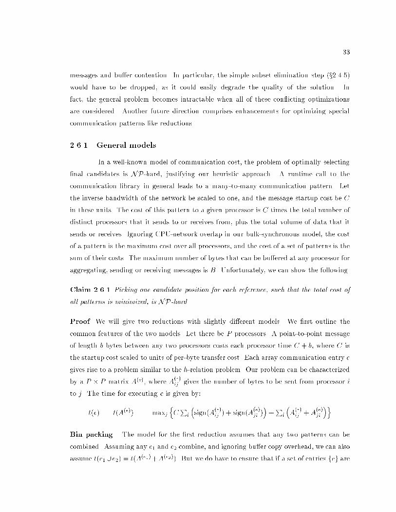
33
messages and bu�er contention. In particular, the simple subset elimination step (x2.4.5)would have to be dropped, as it could easily degrade the quality of the solution. In
fact, the general problem becomes intractable when all of these con icting optimizations
are considered. Another future direction comprises enhancements for optimizing special
communication patterns like reductions.
2.6.1 General models
In a well-known model of communication cost, the problem of optimally selecting
�nal candidates is NP-hard, justifying our heuristic approach. A runtime call to the
communication library in general leads to a many-to-many communication pattern. Let
the inverse bandwidth of the network be scaled to one, and the message startup cost be C
in these units. The cost of this pattern to a given processor is C times the total number of
distinct processors that it sends to or receives from, plus the total volume of data that it
sends or receives. Ignoring CPU-network overlap in our bulk-synchronous model, the cost
of a pattern is the maximum cost over all processors, and the cost of a set of patterns is the
sum of their costs. The maximum number of bytes that can be bu�ered at any processor for
aggregating, sending or receiving messages is B. Unfortunately, we can show the following.
Claim 2.6.1 Picking one candidate position for each reference, such that the total cost of
all patterns is minimized, is NP-hard.
Proof. We will give two reductions with slightly di�erent models. We �rst outline the
common features of the two models. Let there be P processors. A point-to-point message
of length b bytes between any two processors costs each processor time C + b, where C is
the startup cost scaled to units of per-byte transfer cost. Each array communication entry e
gives rise to a problem similar to the h-relation problem. Our problem can be characterized
by a P � P matrix A(e), where A
(e)ij
gives the number of bytes to be sent from processor i
to j. The time for executing e is given by:
t(e) = t(A(e)) = maxj
nCP
i
�sign(A
(e)ij) + sign(A
(e)ji)
�+
Pi
�A(e)ij
+ A(e)ji
�o
Bin packing. The model for the �rst reduction assumes that any two patterns can be
combined. Assuming any e1 and e2 combine, and ignoring bu�er copy overhead, we can also
assume t(e1[e2) = t(A(e1)+A(e2)). But we do have to ensure that if a set of entries feg are
34
combined, no processor bu�ers more than B bytes for sending or receiving. It is trivial to
reduce bin-packing to this problem. Let there be communication only from processor 1 to 2;
and let the number of bytes in the messages be the item sizes from the bin-packing problem,
and let the bu�er limit be the bin size. Minimizing the number of bins then corresponds to
the minimum number of messages.
Set cover. In practice, code generation issues make it impossible to combine arbitrary
entries e1 and e2. The second model ignores the bu�er constraint B and focuses on the
communication pattern; speci�cally, assume that similar to x2.4.7, we combine entries
e1 = hD1;M1i and e2 = hD2;M2i i� M1 �M2 or M2 �M1.
Initially make the temporary assumption that sending message is free, and
receiving message has some enormous startup cost. Under this model, the cost of an entry is
the maximum number of messages any processor receives. If sending also had large startup
cost, the cost of an entry would be the maximum number of messages any processor sends
plus receives.
Given a set cover instance with elems fe1; : : : ; eng and sets fS1; : : : ; Smg. Elemsare assigned numbers 1; : : : ; n. We will have n + m entries. Each entry is P � P where
P = n + 1. For each element j there is an entry cj of the following form: cj [0; j] = 1; all
other cj [ ] = 0. For every set Si there is also an entry: ci[0; j] = 1 i� j 2 Si. All other
ci[ ] = 0. The rules for combining are as above. We say two entries c1 and c2 are combinable
i� elementwise c1 � c2 or c2 � c1. If there is a set cover of size K, then there is a message
schedule with K messages, and conversely. It is not only NP-hard to solve set cover exactly,but there is a constant c such that it is not possible to get a polynomial time algorithm that
returns a solution within a multiplicative factor of c logn of optimum, unless P = NP .The reason for the temporary assumption was that otherwise processor 0 would
have to send many messages, while all other processors receive one message each in parallel
for every entry. To remove the assumption, just stagger the �rst row of each matrix: instead
of setting c[0; j] to 1, set c[j � 1; j] to 1. Now for each entry each processor has to send at
most one message and receive at most one message. By blowing up P by a factor of 2, we
can even make sure that no processor both sends and receives.
Like many other NP-hard problems, the optimization problem can be formulated
as an integer linear program (ILP). Furthermore, several additional constraints can be
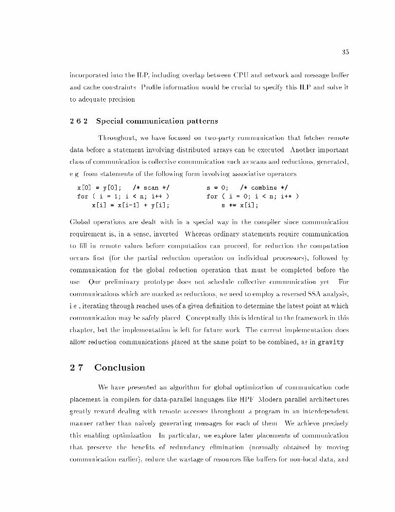
35
incorporated into the ILP, including overlap between CPU and network and message bu�er
and cache constraints. Pro�le information would be crucial to specify this ILP and solve it
to adequate precision.
2.6.2 Special communication patterns
Throughout, we have focused on two-party communication that fetches remote
data before a statement involving distributed arrays can be executed. Another important
class of communication is collective communication such as scans and reductions, generated,
e.g. from statements of the following form involving associative operators.
x[0] = y[0]; /* scan */ s = 0; /* combine */
for ( i = 1; i < n; i++ ) for ( i = 0; i < n; i++ )
x[i] = x[i-1] + y[i]; s += x[i];
Global operations are dealt with in a special way in the compiler since communication
requirement is, in a sense, inverted. Whereas ordinary statements require communication
to �ll in remote values before computation can proceed, for reduction the computation
occurs �rst (for the partial reduction operation on individual processors), followed by
communication for the global reduction operation that must be completed before the
use. Our preliminary prototype does not schedule collective communication yet. For
communications which are marked as reductions, we need to employ a reversed SSA analysis,
i.e., iterating through reached uses of a given de�nition to determine the latest point at which
communication may be safely placed. Conceptually this is identical to the framework in this
chapter, but the implementation is left for future work. The current implementation does
allow reduction communications placed at the same point to be combined, as in gravity.
2.7 Conclusion
We have presented an algorithm for global optimization of communication code
placement in compilers for data-parallel languages like HPF. Modern parallel architectures
greatly reward dealing with remote accesses throughout a program in an interdependent
manner rather than naively generating messages for each of them. We achieve precisely
this enabling optimization. In particular, we explore later placements of communication
that preserve the bene�ts of redundancy elimination (normally obtained by moving
communication earlier), reduce the wastage of resources like bu�ers for non-local data, and
36
improve performance due to other factors like fewer messages. Preliminary performance
results obtained on some HPF benchmarks show signi�cant reduction in communication
costs and overall improvements in performance of those programs on the IBM SP2 and
a cluster of Sparcs connected by Myrinet. In the future, we will conduct performance
studies to investigate the desirability of including partial redundancy elimination as well
into our framework. Another area for future work is interprocedural analysis; we believe
that the application of our algorithm across procedure boundaries can often lead to further
improvements in performance.
37
Chapter 3
Scheduling hybrid parallelism
3.1 Introduction
The parallel executable code that compilers for data parallel languages generate
usually runs in a bulk synchronous style. There are alternating phases of computation
and cooperative communication across most or all processors. Fine-grain asynchronous
communication is expensive on most current machines. Reducing this is an active area
of parallel architecture research. However, it is also important for compilers and runtime
systems to optimize an application to coarsen the grain size and make the communication
more coordinated. The compiler algorithm outlined in the previous chapter enhances the
bulk-synchrony of the program. Another way to reduce communication overhead is to
reduce the number of processors, which makes sense only if the application has other
work that can be done on the freed processors. In the context of data-parallel languages
like High Performance Fortran (HPF), this is equivalent to applications that show task
parallelism as well as the standard data parallelism of loops. There is a growing body of
such applications, including eigensolvers, adaptive mesh codes, circuit simulation, and query
trees in parallel relational databases. Another incentive for investigating such programming
models is that future multiprocessors are likely to be clusters of symmetric shared memory
(SMP) machines. The data and task parallelism will map e�ciently to within and across
SMP clusters, since loop-level communication in data parallelism can be supported by
shared memory, while relatively infrequent task-level communication can be implemented
via message passing across clusters.
Recent versions of the HPF proposal includes support for such applications [55].
38
Some parallelizing compilers have been extended to express such a mixed parallel execution
model, but the algorithmic details of the runtime scheduler are still under debate. These
applications are characterized by a precedence graph of tasks, each of which can run on many
processors in a data parallel fashion. For applications amenable to compile-time scheduling,
the task graph has to be known statically, and information about the communication and
computation cost of all the task nodes is needed.
Unfortunately, the amount of static task parallelism in most problems is so small
(typically 4{8) that except for the smallest problems, the gains over pure data parallelism
are negligible. Static task graphs, such as those generated from control ow graphs
by parallelizing compilers, have a �xed small degree of task parallelism. For example,
the benchmarks in [95] have 4{7 fold e�ective task parallelism and the signal processing
applications in [110] have a 2{5 fold task parallelism. The task parallelism in climate
modeling applications is typically no more than 4{6.
Problems where the task parallelism grows with problem size, such as divide and
conquer problems, are therefore much more promising from the perspective of exploiting
mixed parallelism, and are the focus of this chapter. On the other hand, these applications
may have to be scheduled dynamically, because the structure of the task graph and costs of
tasks may not be known in advance. With runtime scheduling, the ability to use expensive
optimization techniques, such as linear-programming, is limited. This chapter explores
how to extend the purely data-parallel execution model of HPF and implement simple and
e�ective dynamic scheduling algorithms. Speci�cally, we make the following contributions:
� We identify the nature of applications that need task parallelism in addition to data
parallelism for enhanced performance. In particular, we focus on dynamic, scalable
task parallelism such as in divide and conquer.
� For dynamic scenarios, we formulate and give practical solutions for scheduling such
task graphs using a simple switched execution strategy: some tasks are allocated all
processors, some only one; the system alternates between executing tasks of the �rst
type one after the other, and packing tasks of the second type into the processors
evenly.
� We prove that the algorithms are close to the best possible switched execution. We also
show by experiments that the gains of switched parallelism over pure data-parallelism
39
can be dramatic, e.g., up to a factor of three times higher MFLOPS on the IBM SP2.
(This 3� factor is not to be compared with the 2{7� task parallelism mentioned
earlier; those amounts of statically available task parallelism do not translate into
similar improvements over data parallelism.)
� Using simulation we estimate the gap between the e�ciency of switched parallel
execution with the best possible e�ciency of any scheduler. The gap is small.
Data parallelism is the most familiar parallel execution model in scienti�c
computing, as in ScaLAPACK, CMSSL, FortranD, CM-Fortran, and High Performance
Fortran [45, 76, 72, 49, 55]. The computational load can usually be balanced statically, and
the important performance issue is generating parallel loops with minimal communication
overhead (as in Chapter 2). In general, data parallel applications show cooperative
computation and communication within loops, and the parallelism in an operation is
exploited over the complete machine partition.
Task parallelism is speci�ed at the language level using statements like \fork",
which generate a new thread of control to execute the given function invocation. Tasks
may depend on the completion of other tasks, so task parallelism is modeled by an acyclic
graph (DAG) whose vertices represent tasks. Each task runs on exactly one processor (i.e.,
is sequential). The advantage is that communication is potentially required only in setting
up the task and retrieving outputs. Since the task runs on one processor, no inter-processor
communication occurs during task execution. (In our problem domain we do not need to
deal with inter-process communication on the same processor.) The challenge is that often
no information about the structure of the task graph or the cost of tasks is available at
compile-time, making load balancing a more di�cult runtime problem.
3.2 Notation
We will model mixed parallel applications as macro-data ow graphs [95]. Each
vertex of the (directed acyclic) graph represents a data-parallel task, which could be written
using HPF or ScaLAPACK. The edges represent data and/or control dependency. In this
chapter we will assume some advance knowledge of a task's running time given the number
of processors it is allocated, at the time the task arrives, at the latest. The most general
form in which this can be speci�ed is function tj(�), which gives the running time of task
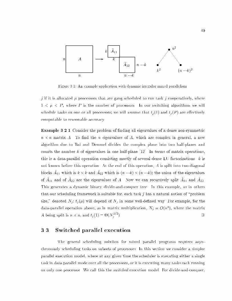
40
. . . . . . . . . . . . . . . . .
. . . . . . . . . . . . . . . . .
..
..
..
..
..
..
..
..
.
..
..
..
..
..
..
..
..
.
-A
eA11
eA22
n
n
k
k
n � k
n� k
n2
k2 (n� k)2
Figure 3.1: An example application with dynamic irregular mixed parallelism.
j if it is allocated � processors that are gang scheduled to run task j cooperatively, where
1 < � < P , where P is the number of processors. In our switching algorithms we will
schedule tasks on one or all processors; we will assume that tj(1) and tj(P ) are e�ectively
computable to reasonable accuracy.
Example 3.2.1 Consider the problem of �nding all eigenvalues of a dense non-symmetric
n � n matrix A. To �nd the n eigenvalues of A, which are complex in general, a new
algorithm due to Bai and Demmel divides the complex plane into two half-planes and
counts the number k of eigenvalues in one half-plane [12]. In terms of matrix operations,
this is a data-parallel operation consisting mostly of several dense LU factorizations. k is
not known before this operation. At the end of this operation, A is split into two diagonal
blocks ~A11 which is k � k and ~A22 which is (n� k)� (n� k); the union of the eigenvalues
of ~A11 and of ~A22 are the eigenvalues of A. Now we can recursively split ~A11 and ~A22.
This generates a dynamic binary divide-and-conquer tree. In this example, as in others
that our scheduling framework is suitable for, each task j has a natural notion of \problem
size," denoted Nj; tj(�) will depend of Nj in some well-de�ned way. For example, for the
data-parallel operation above, as in matrix multiplication, Nj = O(n2), where the matrix
A being split is n� n, and tj(1) = �(N3=2j
). 2
3.3 Switched parallel execution
The general scheduling solution for mixed parallel programs requires asyn-
chronously scheduling tasks on subsets of processors. In this section we consider a simpler
parallel execution model, where at any given time the scheduler is executing either a single
task in data parallel mode over all the processors, or it is executing many tasks each running
on only one processor. We call this the switched execution model. For divide-and-conquer,
41
there is in fact only one switch point: large tasks near the root of the divide-and-conquer
tree run in data parallel mode; the remaining tasks are packed into a task parallel mode.
Switching is simple to program and, for divide-and-conquer, has only one global
data remapping phase. General processor subset scheduling may have better processor
utilization but has much higher communication and synchronization overhead. In this
section, we will give simple heuristics to schedule tasks in such a model, and prove some
bounds on their performance. Then in x3.4, we study how close the performance of this
restricted model is to the best possible. We set up the switching problem as follows.
Input. There is a set J of n tasks and P processors. These tasks have data parallelism.
Task j speci�es running times under two settings: on one processor, it takes time tj(1)
run in task-parallel fashion; on all P processors it takes time tj(P ) to run in data-parallel
fashion. (Usually tj(P ) � t1(P )=P , but we will not need this property.) The tasks may be
independent as in x3.3.1, or there may be certain precedence restrictions between them, as
in x3.3.2.
Model. We wish to minimize the execution time of a schedule with the following structure.
The tasks are classi�ed (partitioned) into two groups, JP and J1. Tasks in JP are run one
after the other in some order consistent with the precedence restrictions, allocating to each
task all the P processors. Let the total time for this phase be tP . Each task in J1 is run
on one processor. They can run concurrently with each other, again as long as precedence
restrictions are not violated. Let the total time for this phase be t1. The total execution
time is tP + t1.
Classi�cation. The classi�cation problem is to �nd JP and J1 such that there is a
two-phase schedule of optimal makespan where JP is executed in data parallel mode and
J1 is executed in task parallel mode.
Scheduling. Given JP and J1, the problem is to compute a good schedule. Note
that scheduling JP is trivial, and Graham's list scheduling su�ces for J1. Even after
classi�cation, constructing an optimal schedule is clearly NP-hard via reduction from
partition. It is easy to see that even the classi�cation is NP-hard.
Claim 3.3.1 The classi�cation problem is NP-hard, even for independent tasks.
42
Proof. By reducing partition to the classi�cation problem. Given a partition instance
A = fa1; : : : ; ang, where these are positive integers, let there be P = 2 processors and n
tasks, task j having tj(1) = aj and tj(P ) =aj
2+ � for suitably small � > 0. If there is a
partition of A, then the best classi�cation is task-parallel for all tasks. If a partition of A
does not exist, then the best classi�cation is data-parallel for all tasks.
However, it is often possible to classify tasks to achieve near-optimal makespan, as
we see next. Thereafter we can use a standard list-type near-optimal scheduling algorithm
to get an overall schedule within a small constant factor of the optimal switched schedule,
in the worst case.
3.3.1 Switching a batch
The input instance is a set J of independent tasks. Task i has sizeNi and sequential
running time ti(1) = f(Ni) which increases with Ni. Assume all Ni are large enough that
ti(1) > ti(P ) (otherwise these small tasks would clearly be better o� in the task parallel
phase). The problem is to decide for each whether to execute it in data parallel mode or
task parallel mode. It is clear that there is an optimal switched schedule that switches
exactly once between the data-parallel and task-parallel phase.
A �rst cut solution is to de�ne JP = fj : tj(P ) < tj(1)g; this has been used
in practice [17]. This is overly conservative since it does not consider the complete ready
list to decide the fate of a single task. We use the following algorithm: sort the tasks in
decreasing order of problem size, and �nd an index j such that the total time of executing
tasks 1; : : : ; j one after the other in data parallel mode followed by tasks j + 1; : : : ; jJ j in a
task parallel packing is minimized.
Let Pack(P; S) be the makespan (length of schedule) generated by packing tasks
from set S in task parallel mode into P processors. There are approximation algorithms
that return Pack � (1 + �)PackOPT for any �xed � > 0, within time that is polynomial in
jSj [104]. Here PackOPT is the optimal makespan. It is easy to see that PackOPT(P; S) �1P
Ps2S ts(1) + maxs2S ts(1), by an averaging argument. Consider the following heuristic,
which we call Pre�x-Su�x.
1. Sort tasks in decreasing order of tj(1); i.e., let t1(1) � t2(1) � � � � � tL(1).
43
2. For 1 � i � L + 1, de�ne p[i] =
P1�j<i tj(P ) (p[1] = 0), and de�ne s[i] =
Pack(P; fi; : : : ; Lg) (s[L+ 1] = 0).
3. Pick 1 � i� � L+1 such that p[i�]+s[i�] is minimal over all i, such that 1 � i � L+1.
4. Run tasks 1; : : : ; i��1 in data parallel mode, and tasks i�; : : : ; L in task parallel mode.
For the analysis, consider a modi�ed problem where tasks i; : : : ; L have to be
scheduled using switched parallelism, given the constraint that the largest task i has to be
run during the task parallel phase. Let s�[i] be the optimal switched makespan subject to
this new constraint.
Lemma 3.3.2 PackOPT(P; fi; : : : ; Lg) � 2 s�[i].
Proof. Because PackOPT(P; fi; : : : ; Lg) � 1P(ti(1) + � � � + tL(1)) + ti(1), and s�[i] �
maxf 1P(ti(1) + � � �+ tL(1)); ti(1)g.
Theorem 3.3.3 Independent tasks can be classi�ed in polynomial time such that the
resulting makespan is within a factor of (2+ �) of the makespan of the optimal schedule, for
arbitrary constant � > 0.
Proof. Given an optimal schedule, let ` be the smallest index in the above sorted order
such that task ` is executed in task parallel mode. Pre�x-Su�x produces a schedule of length
p[i�]+s[i�] � p[`]+s[`] = p[`]+Pack(P; f`; : : : ; Lg) � p[`]+(1+�) PackOPT(P; f`; : : : ; Lg) �p[`] + 2 (1+ �) s�[`] � 2 (1 + �) (p[`] + s�[`]) = 2 (1 + �) OPT, since OPT � p[`] + s�[`].
In a dynamic divide-and-conquer tree, we assume that the problem size of tasks
decreases down any path in the tree. For such trees, we can proceed as follows.
1. Maintain a ready-list of independent tasks/tasks that have been generated but not
executed yet.
2. Before scheduling a module in data parallel mode, apply the above pre�x-su�x
heuristic to the ready-list of tasks.
3. If the best data parallel pre�x is empty, decide to switch to task parallelism at this
point.
44
This is only a heuristic, since in the worst case, an adversary can prune all but the largest
task on the frontier immediately after the algorithm decides to switch. While this means
that we have no provable bounds, such malicious behavior is rare in practice. We will show
that this heuristic performs quite well in x3.5.
3.3.2 Precedence graphs
In contrast to dynamic trees, if the precedence graph is a tree and is known
before startup, we can provide a simple polynomial time constant factor algorithm. It uses
dynamic programming and is very inexpensive compared to mathematical programming
type approaches.
The problem instance is a set of n tasks, each task j specifying tj(1) and tj(P )
as before. We will consider schedules with one switch: the large nodes at and near the
tree root are processed in fully parallel mode, and then a switch is made to task-parallel
execution of the remaining nodes.
De�nition 3.3.4 For task j in a directed acyclic precedence relation �, PathToLeaf(j) =tj(1) + maxj�i PathToLeaf(i), and PathToRoot(j) = tj(1) + maxi�j PathToRoot(i).
We will do binary search for the makespan between a lower and upper bound
similar to the classical �-approximate decision procedures [104]. Suppose in the current
search step the proposed deadline is D.
1. Compute PathToLeaf(j) by a bottom-up traversal. Compute SP = fj :
PathToLeaf(j)� tj(1) > Dg. If Pj2SP tj(P ) > D then deadline D is infeasible.
2. We will solve a certain knapsack-like problem. The items to pack are tasks, these are
assigned pro�ts and weights. The knapsack has a weight limit; the goal is to maximize
the pro�t of items packed. Let the pro�t of task j be tj(1), and the weight be tj(P ).
Obtain S0P= Knapsack(J;D) having total weight at most (1+�)D such that the pro�t
is at least that of the optimal knapsack packing. The algorithm Knapsack has been
described in Chapter 4, x?? (page 82).
3. If
Pj 62S0
Ptj(1) > D � P then deadline D is not feasible.
45
4. Execute SP [ S0Pon all P processors in any order consistent with the precedence
constraints given by the tree edges. List schedule the remaining tasks in task parallel
fashion.
Lemma 3.3.5 If deadline D is feasible, the above schedule terminates in time (4 + �)D.
Proof. If D is feasible, then
Pj2SP[S0P tj(P ) � (2 + �)D. Also by a standard critical path
argument the time to execute all j 62 SP [ S0P using list scheduling is at mostXj 62SP[S0P
tj(1) + max
j 62SP[S0PPathToLeaf(j) � 2D:
Theorem 3.3.6 A single switch point for a task tree can be found that gives makespan
within a factor of (4+ �) of the optimal switch, for an arbitrarily small constant � > 0. The
algorithm takes time polynomial in 1=� and the number of tasks.
One can solve series-parallel task graphs in a similar fashion. Notice the \single"
clause; clearly, if tj(1) and tj(P ) are arbitrary, a single switch can be very bad. However,
tree precedences are most common in divide and conquer problems, where problem sized
decreases monotonically down any path from the root; thus for any P and j1 � j2, the
e�ciency of running j1 on P processors is at least that of j2. Under this realistic condition
it is easy to see that one switch makespan is within a factor of two of many switches.
While these worst-case factors are small, they may mask the bene�ts of investing in
mixed parallelism in the �rst place. Therefore, we will need to supplement these worst-case
results by simulations and actual implementation. This we do next.
3.4 Modeling and analysis
In this section we will obtain analytical and empirical results that indicate that
the switched scheduling model achieves e�ciency quite close to the best possible, in our
context of divide-and-conquer problems. For this we will develop a model in two parts:
1. We propose a model for the e�ciency of a data parallel module as a function of N=P ,
the \problem size per processor."
2. We model regular divide-and-conquer trees in terms of the out-degree d and the shrink
factor c, the ratio of the problem size of a parent to that of a child.
46
3.4.1 E�ciency of data parallelism
If all the data parallel modules j at the nodes of the task graph where ideally
scalable, i.e., had tj(�) = tj(1)=� for � as large as P , the number of processors in the
machine, then using mixed or switched parallelism is a non-issue. The gains from extending
beyond pure data parallelism are a function of how poorly scalable the data parallel modules
are. In this section we propose an e�ciency model for a data parallel module.
We let e(N;P ) be the parallel e�ciency of solving a problem of size N on P
processors. Informally, the \size" N of a problem or task is the total data volume, e.g., for
n � n matrix multiplication, N = �(n2). If the serial running time is f(N), the parallel
running time r(N;P ) on P processors is r(N;P ) = f(N)=(P �e(N;P )). e(N;P ) depends onthe algorithm, and relative speeds of computation and communication. Despite e's possibly
complex dependence on all these parameters, we will show that for a number of algorithms of
interest, e(N;P ) is accurately modeled by a simple two-parameter function of the problem
size per processor, N=P .
By Amdahl's law, we expect e to be a decreasing function of P , with e(�; 1) = 1. So
our intuition is that e(N;P ) should be an increasing function of N=P . We will let e1 � 1
be its asymptotic value for large N=P . The next question is how e(N;P ) approaches e1.
There are, of course, an in�nite number of functions to model this, but we shall propose
a simple model that we will empirically validate. Roughly speaking, the model captures
programs having an area-to-volume relationship between communication and computation,
which abounds in parallel scienti�c applications.
3.4.1.1 A proposed model
One model we have found to agree very closely with experimental data is the
following. The e�ciency of a data parallel task of size N on P processors is modeled as
e(N;P ) =
8><>:
1 if P = 1
e11 + �P=N
if P > 1.
(3.1)
The parameter � measures how fast the e�ciency approaches its asymptotic value e1. As
shown in Figure 3.2 the e�ciency reaches half its asymptotic value when N=P = �. Thus,
the smaller the value of �, the more e�cient the implementation is for a �xed problem size.
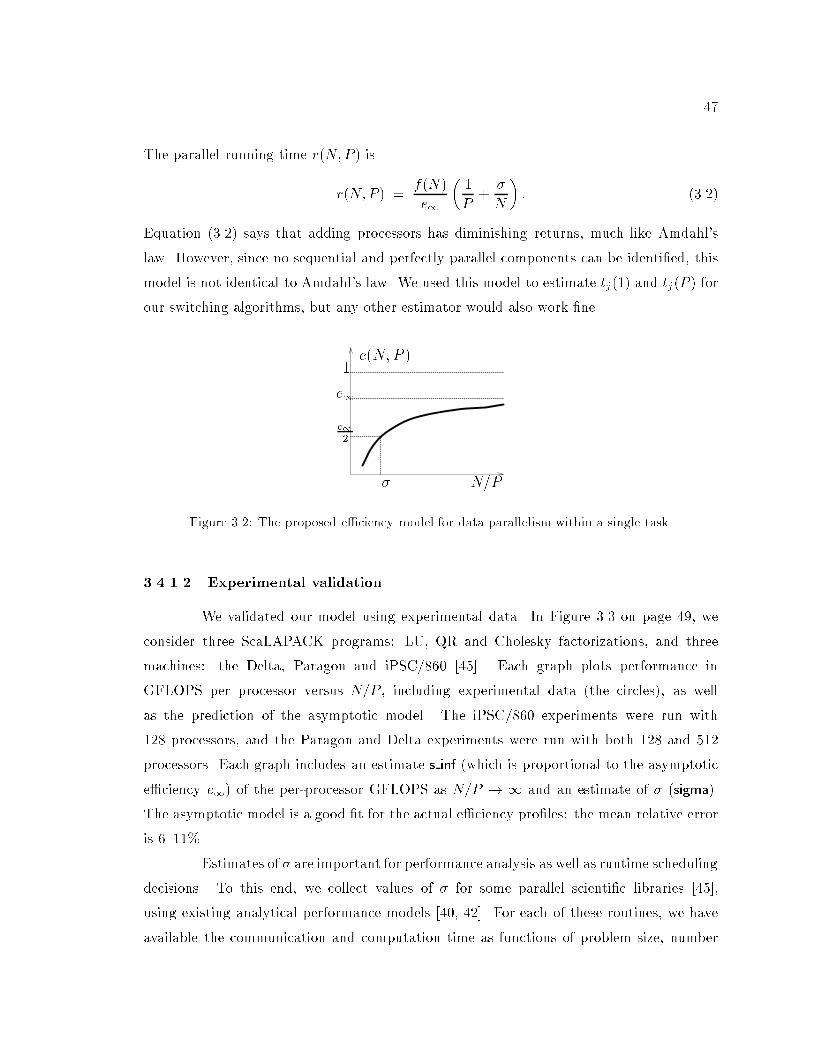
47
The parallel running time r(N;P ) is
r(N;P ) =f(N)
e1
�1
P+
�
N
�: (3.2)
Equation (3.2) says that adding processors has diminishing returns, much like Amdahl's
law. However, since no sequential and perfectly parallel components can be identi�ed, this
model is not identical to Amdahl's law. We used this model to estimate tj(1) and tj(P ) for
our switching algorithms, but any other estimator would also work �ne.
N=P�
e(N;P )1
e1
e1
2
Figure 3.2: The proposed e�ciency model for data parallelism within a single task.
3.4.1.2 Experimental validation
We validated our model using experimental data. In Figure 3.3 on page 49, we
consider three ScaLAPACK programs: LU, QR and Cholesky factorizations, and three
machines: the Delta, Paragon and iPSC/860 [45]. Each graph plots performance in
GFLOPS per processor versus N=P , including experimental data (the circles), as well
as the prediction of the asymptotic model. The iPSC/860 experiments were run with
128 processors, and the Paragon and Delta experiments were run with both 128 and 512
processors. Each graph includes an estimate s inf (which is proportional to the asymptotic
e�ciency e1) of the per-processor GFLOPS as N=P ! 1 and an estimate of � (sigma).
The asymptotic model is a good �t for the actual e�ciency pro�les: the mean relative error
is 6{11%.
Estimates of � are important for performance analysis as well as runtime scheduling
decisions. To this end, we collect values of � for some parallel scienti�c libraries [45],
using existing analytical performance models [40, 42]. For each of these routines, we have
available the communication and computation time as functions of problem size, number
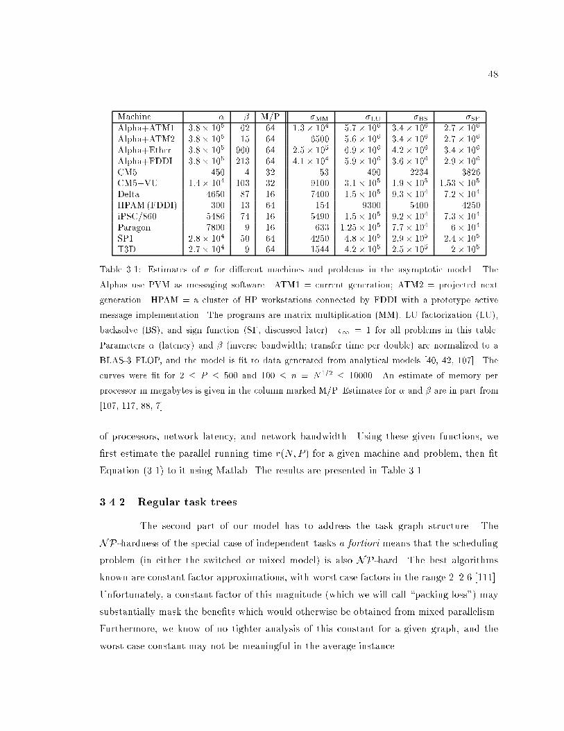
48
Machine � � M/P �MM �LU �BS �SFAlpha+ATM1 3:8� 105 62 64 1:3� 104 5:7� 106 3:4� 106 2:7� 106
Alpha+ATM2 3:8� 105 15 64 6500 5:6� 106 3:4� 106 2:7� 106
Alpha+Ether 3:8� 105 960 64 2:5� 105 6:9� 106 4:2� 106 3:4� 106
Alpha+FDDI 3:8� 105 213 64 4:1� 104 5:9� 106 3:6� 106 2:9� 106
CM5 450 4 32 53 490 2234 3826CM5+VU 1:4� 104 103 32 9100 3:1� 105 1:9� 105 1:53� 105
Delta 4650 87 16 7400 1:5� 105 9:3� 104 7:2� 104
HPAM(FDDI) 300 13 64 154 9300 5400 4250iPSC/860 5486 74 16 5490 1:5� 105 9:2� 104 7:3� 104
Paragon 7800 9 16 633 1:25� 105 7:7� 104 6� 104
SP1 2:8� 104 50 64 4250 4:8� 105 2:9� 105 2:4� 105
T3D 2:7� 104 9 64 1544 4:2� 105 2:5� 105 2� 105
Table 3.1: Estimates of � for di�erent machines and problems in the asymptotic model. The
Alphas use PVM as messaging software. ATM1 = current generation; ATM2 = projected next
generation. HPAM = a cluster of HP workstations connected by FDDI with a prototype active
message implementation. The programs are matrix multiplication (MM), LU factorization (LU),
backsolve (BS), and sign function (SF, discussed later). e1 = 1 for all problems in this table.
Parameters � (latency) and � (inverse bandwidth; transfer time per double) are normalized to a
BLAS-3 FLOP, and the model is �t to data generated from analytical models [40, 42, 107]. The
curves were �t for 2 � P � 500 and 100 � n = N1=2� 10000. An estimate of memory per
processor in megabytes is given in the column marked M/P. Estimates for � and � are in part from
[107, 117, 88, 7].
of processors, network latency, and network bandwidth. Using these given functions, we
�rst estimate the parallel running time r(N;P ) for a given machine and problem, then �t
Equation (3.1) to it using Matlab. The results are presented in Table 3.1.
3.4.2 Regular task trees
The second part of our model has to address the task graph structure. The
NP-hardness of the special case of independent tasks a fortiori means that the scheduling
problem (in either the switched or mixed model) is also NP-hard. The best algorithms
known are constant factor approximations, with worst case factors in the range 2{2.6 [111].
Unfortunately, a constant factor of this magnitude (which we will call \packing loss") may
substantially mask the bene�ts which would otherwise be obtained from mixed parallelism.
Furthermore, we know of no tighter analysis of this constant for a given graph, and the
worst case constant may not be meaningful in the average instance.
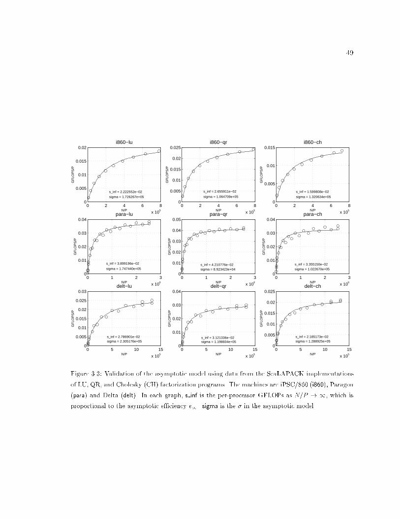
49
0 2 4 6 8
x 105
0
0.005
0.01
0.015
0.02
s_inf = 2.222552e−02
sigma = 1.726267e+05
i860−lu
N/P
GF
LOP
S/P
0 2 4 6 8
x 105
0
0.005
0.01
0.015
0.02
0.025
s_inf = 2.655911e−02
sigma = 1.064709e+05
i860−qr
N/P
GF
LOP
S/P
0 2 4 6 8
x 105
0
0.005
0.01
0.015
s_inf = 1.599808e−02
sigma = 1.320634e+05
i860−ch
N/P
GF
LOP
S/P
0 1 2 3
x 106
0
0.01
0.02
0.03
0.04
s_inf = 3.899196e−02
sigma = 1.747440e+05
para−lu
N/P
GF
LOP
S/P
0 1 2 3
x 106
0
0.01
0.02
0.03
0.04
0.05
s_inf = 4.210776e−02sigma = 8.923423e+04
para−qr
N/P
GF
LOP
S/P
0 1 2 3
x 106
0
0.01
0.02
0.03
0.04
s_inf = 3.355150e−02sigma = 1.022670e+05
para−ch
N/P
GF
LOP
S/P
0 5 10 15
x 105
0
0.005
0.01
0.015
0.02
0.025
0.03
s_inf = 2.786901e−02sigma = 2.305176e+05
delt−lu
N/P
GF
LOP
S/P
0 5 10 15
x 105
0
0.01
0.02
0.03
0.04
s_inf = 3.121336e−02sigma = 1.198604e+05
delt−qr
N/P
GF
LOP
S/P
0 5 10 15
x 105
0
0.005
0.01
0.015
0.02
0.025
s_inf = 2.185173e−02sigma = 1.288925e+05
delt−ch
N/P
GF
LOP
S/P
Figure 3.3: Validation of the asymptotic model using data from the ScaLAPACK implementations
of LU, QR, and Cholesky (CH) factorization programs. The machines are iPSC/860 (i860), Paragon
(para) and Delta (delt). In each graph, s inf is the per-processor GFLOPs as N=P ! 1, which is
proportional to the asymptotic e�ciency e1. sigma is the � in the asymptotic model.
50
3.4.2.1 Model
We therefore consider how mixed parallelism will perform in very favorable
circumstances, namely in regular divide and conquer trees. Our assumptions are listed
below.
� The task graph is a complete tree with branching factor d � 2.
� The d child tasks of a task of size N are all of size N=c, where c > 1.
� The work required to do a task of size N is f(N) = Na, where a � 1.
We call such regular trees that have a root size of N as (N; a; c; d) trees. This is a very
simple model, and so we need to understand the limits of its applicability. First, task
communication is not accounted for. But for a > 1, task communication cost is generally
of lower order than the node cost f(N) (e.g., O(N) vs. O(N3=2) in the case of many dense
matrix operations). Thus, we expect our model to overestimate the bene�ts of mixed
parallelism, provided problems are large enough. Therefore, a prediction of little bene�t
frommixed parallelism for a particular problem is likely to be trustworthy, while a prediction
of great bene�t from mixed parallelism must be further analyzed. Second, for evaluating
e�ciency gains with high accuracy, only regular trees could be considered. In spite of their
simplicity, regular trees provide a good starting point for preliminary analysis [18].
3.4.2.2 Examples
Eigenvalue algorithms. Several eigenvalue algorithms exhibit mixed parallelism because
they use divide and conquer. One such algorithm was described in Example 3.2.1 on page 40.
If the divide step on a matrix of size N = n2 is perfect, each child is of sizen
2 � n
2 , or N=4.
Performing this separation requires O(N3=2) FLOPS. This successive separation process
forms a binary tree with c = 4, d = 2, and a = 3=2. (We scale time so that the constant in
O(N3=2) becomes one.)
For symmetric matrices, an algorithm similar in spirit is the beta-function
technique of Bischof et al [17]. An eigenvalue algorithm of a di�erent avor, but still from
the divide and conquer category, is Cuppen's method for symmetric tridiagonal matrices,
where we can actually split the matrix exactly in half all the time [38, 99] (although the
costs of the children are not so simple).
51
Sparse Cholesky. We consider the regular but important special case of the matrix
arising from the 5-point Laplacian on a square grid, ordered using the nested dissection
ordering [60]. In this case one may think of dividing the matrix into 4 independent
subproblems, corresponding to dividing the square grid into 4 subsquares, each of half
the perimeter. The work performed at a node which corresponds to an n�n grid is O(n3);
most of this cost is a dense Cholesky of a small n�n submatrix corresponding to the nodes
on the boundaries of the subsquares. Thus N = n2, a = 3=2, c = 4 and d = 4. We will also
see that the results go over to matrices with planar graphs.
3.4.3 Analysis
We make some simple observations about batches of independent tasks. For a
single task with sequential running time f(N), the choice is only between 1 and P processors,
and the running time is
f(N) � min
�1
e1
�1
P+
�
N
�; 1
�
For a batch of L independent tasks, each of size N , the sequential running time t1
of all L tasks is Lf(N). The data parallel running time tD, where we run each task in data
parallel fashion one after the other, is just L times the above expression. We let tT denote the
task parallel running time, where we assign one processor per task. Finally, we let tM denote
the mixed parallel running time, the optimal running time over all possible assignments of
processors to tasks. Let eD, eS , and eM be the corresponding overall e�ciencies.
By allocating only one processor per task, we can get parallel execution time
dL=Pef(N). Since the work lower bound is Lf(N)=P , pure task parallelism is optimal
when L � P (modulo rounding e�ects, which we ignore here and elsewhere). Thus, we
need only consider the case L < P . Also assume L divides P . We note the following easy
observations.
1. When L divides P , the running time for L independent tasks of size N in the asymp-
totic model using optimal mixed parallelism is tM = f(N)�min
n1; 1
e1
�L
P+
�
N
�o,
2. When L divides P , the running time using data parallelism is tD = L f(N) �min
n1; 1
e1
�1P+
�
N
�o.
52
3. When task parallelism is not optimal, the relative improvement of using mixed
parallelism over pure data parallelism for the batch problem is
eM
eD=
N
�P+ 1
N
�P+
1L
(3.3)
Example 3.4.1 We apply this analysis to complex matrix multiplication, which was
reported as a benchmark for the Illinois Paradigm compiler [95]. The task is MM, the
machine is the CM5 without vector units, and L = 4. From Figure 3.1 we obtain � = 53
and e1 = 1 for this problem. To attain a relative improvement � of mixed over data
parallelism, i.e. eD=eM < 1� �, we need the problem size to be small. Speci�cally, if each
MM involves n�n matrices, we can substitute the numbers into (3.3) and see that n needs
to be less than roughly
p53P (3� 4�)=4� for this improvement. E.g., if P = 64 and � = 0:5,
then n < 42, a tiny problem indeed. It is interesting that the experiments reported in [95]
for the CM5 use P 2 f64; 128g processors and n = 64. On the Paragon with P = 512 and
� = 633, to ensure eD=eM < 0:5 as above, we will need roughly that n < 569, which is
still not large by the standard of many scienti�c applications: a matrix of this size �lls only
0.03% of the Paragon's total memory. 2
The conclusion is that MM data parallelizes too well to bene�t much from mixed
parallelism on a machine as balanced (i.e. with as low a �) as the CM5 without vectors
units. Better hunting grounds for cases where mixed parallelism helps signi�cantly are more
unbalanced machines (high �) and problems with less scalable data parallel components.
Example 3.4.2 Changing the problem to BS (backsolve; solving an n�n upper triangular
system of linear equations) in the last example and changing the machine to a 16 processor
SP1, we see that n < 1386 must hold for eD=eM � 0:5. This is a relatively realistic size.
Mixed parallelism improves the e�ciency from roughly 33% to 66%. 2
3.4.4 Unbalanced batch problems
So far we have considered batches of tasks of identical size N . Here we argue
that permitting tasks of di�erent sizes makes data parallelism only closer in performance to
optimal mixed parallelism, because, if there are a few large tasks that dominate the work
content of the batch, the margin for improvement over pure data parallelism will be small.
53
To prove this, suppose we have a batch of L > 1 tasks, the i-th task of size
Ni. Suppose all tasks have the same e�ciency pro�le e(Ni; P ), and that the sequential
processing time for task i is f(Ni), where f(x) = xa as before. We will need the following
theorem for our proof.
Theorem 3.4.3 (H�older's Inequality) Let xk ; yk > 0 for 1 � k � L, p > 1, and q be
such that 1p+
1q= 1. Then
Xk
xkyk ��X
k
xp
k
�1=p�Xk
yq
k
�1=q:
Let the pure data parallel running time be tD, the optimal switched execution time be tS ,
and the optimal mixed parallel running time be tM (tM � tS � tD). We will show that,
among all possible batches, a balanced batch poses the worst instance for data parallelism
and thus provides the greatest potential for improvement through mixed parallelism. Of
course, certain quantities have to remain invariant over the space of maximization. Two
invariants are possible:
1. The total work
Pif(Ni) = F , a constant.
2. The total size
PiNi = N , a constant.
We will consider both variations.
Lemma 3.4.4 With tD, tM , and f de�ned as above,
eM
eD=
tD
tM� 1
e1+
�P
e1
�Pk f(Nk)=NkPk f(Nk)
�:
Proof. Immediate, using tM � 1P
Pk f(Nk).
The remaining exercise is to bound from above the parenthesized term in the above RHS.
Theorem 3.4.5 Subject to either invariant,
eM
eD� 1
e1
�1 +
�PL
N
�:
Proof. Here we will do a continuous analysis, assuming Ni's are real, rather than integers.
Also assume Ni > 1 to avoid problems near zero.
For constant F , the quantity in parentheses is maximized when all f(Ni) = F=L.
This follows since x=f�1(x) = x1�1=a which is convex for a > 1.
54
For constant N , using p = a=(a� 1) and q = a in Theorem 3.4.3, we obtain
Xk
Na�1k
� 1 ��X
k
Na
k
�1� 1a � L1=a:
Since
PkNa
k� L(N=L)a = Na=La�1, we have
PkNa�1kP
kNa
k
� L1=a�PkNa
k
�1=a � L
N:
This value is achieved when all Nk are set to N=L.
It can be veri�ed that the claim also holds for functions of the form f(x) = x log x, etc., so
the claim is quite broadly applicable. We can trivially get similar bounds on the e�ciency
gap for irregular task graphs by throwing away the dependency information.
Corollary 3.4.6 The maximum bene�t from mixed parallelism for a task graph G with L
vertices such that the sum of problem sizes is N can be bounded as
eM
eS� eM
eD� 1
e1
�1 +
�PL
N
�;
in the asymptotic model using P processors.
We can also derive some heuristic bounds to the performance gap in some irregular
graphs. E.g., Gilbert and Tarjan study nested dissection algorithms to solve sparse systems
on planar graphs [62], where a problem of size N is divided into d = 2 subproblems, where
each part is no bigger than 2N=3. No matter what strategy we use in the upper levels, we
only need to go down roughly `(�) =lg(�=P )lg(2=3) � 1:71(1� log �
logP ) lgP levels before the largest
leaf is of size at most �N=P . At this point task packing is at most (1 + �) times optimal.
Given that there is not much need to go below this level, L � P 1:71, so the maximum bene�t
cannot be much larger than tS=tM � tD=tM � 1 + �P 2:72=N .
3.4.5 Simulations
As we mentioned earlier, to get accurate estimates of the performance gains from
mixed or switched parallelism, we use simulations based on the data parallel and task graph
models.
Our space of optimal schedules includes those that assign arbitrary subsets of
processors to the tasks. This involves the following runtime support:
55
� It must be possible to create and destroy subsets of the set of physical processor
and rename them in a virtual processor space. These are called contexts in the
Message Passing Interface (MPI) jargon [44]. Note that every message has to be
indirectly addressed to a virtual destination processor, and if many contexts are
de�ned hierarchically, many table-lookups are needed for each message.
� Contexts need to provide synchronization and collective communication primitives,
so that they can be gang-scheduled. These can be potentially expensive. The CM-5,
for example, provides a 5�s hardware barrier over the physical partition, but the best
software barrier over a processor subset takes over 50�s.
In our simulations, we will ignore these overheads, and thus get an upper bound
to the best possible e�ciency, and compare our switched performance against this upper
bound. We will also compare switching with pure data parallelism as in HPF.
Results. The space of programs, machines, and problem sizes is too large to examine
completely; therefore we take some slices through this space that give insight into the
bene�ts of mixed parallelism for typical current architectures and our suite of scienti�c
programs. The following graphs are shown.
1. We �x P = 128, e1 = 1, a = 3=2, and c = d = 4 (as in sparse Cholesky), and
plot eD=eM and eS=eM against � (log-scale) in Figure 3.4. The memory per node
is assumed to be 64MBytes, and the four plots correspond to problem sizes that �ll
25, 50, 75 and 100% of the memory. For typical values of � for various machines see
Table 3.1.
2. For the same sparse Cholesky problem, we consider four machines. In each case, the
x-axis is P . N is such that the memory is completely �lled. We plot eM , eS , and eD
against lg P in Figure 3.5.
3. The setting is as above, except that typical values of P are chosen for each machine
and the x-axis is n = N1=2(log-scale). See Figure 3.6.
4. The setting is as in item (3), but the problem is the sign function program (c = 4,
d = 2). See Figure 3.7. For each task, as a reasonable estimate, there are 15 LU's, 15
BS's and 8 MM's. For this compound data parallel task, estimates of � for various
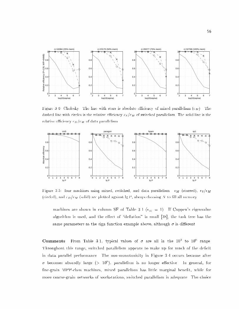
56
2 3 4 5 6 70
0.2
0.4
0.6
0.8
1n=16384 (25% mem)
Rel
ativ
e ef
ficie
ncy
(P=
128,
M/P
=64
MB
)
log10(sigma)2 3 4 5 6 7
0
0.2
0.4
0.6
0.8
1n=23170 (50% mem)
log10(sigma)2 3 4 5 6 7
0
0.2
0.4
0.6
0.8
1n=28377 (75% mem)
log10(sigma)2 3 4 5 6 7
0
0.2
0.4
0.6
0.8
1n=32768 (100% mem)
log10(sigma)
Figure 3.4: Cholesky. The line with stars is absolute e�ciency of mixed parallelism (eM ). The
dashed line with circles is the relative e�ciency eS=eM of switched parallelism. The solid line is the
relative e�ciency eD=eM of data parallelism.
0 1 2 3 4 5 6 7 80
0.2
0.4
0.6
0.8
1
lg P
Abs
olut
e ef
ficie
ncy
cm5
0 1 2 3 4 5 6 7 80
0.2
0.4
0.6
0.8
1
lg P
paragon
0 1 2 3 4 5 6 7 80
0.2
0.4
0.6
0.8
1
lg P
hpam
0 1 2 3 4 5 6 7 80
0.2
0.4
0.6
0.8
1
lg P
sp1
Figure 3.5: four machines using mixed, switched, and data parallelism. eM (starred), eS=eM
(circled), and eD=eM (solid) are plotted against lgP , always choosing N to �ll all memory.
machines are shown in column SF of Table 3.1 (e1 = 1). If Cuppen's eigenvalue
algorithm is used, and the e�ect of \de ation" is small [38], the task tree has the
same parameters as the sign function example above, although � is di�erent.
Comments. From Table 3.1, typical values of � are all in the 102to 10
6range.
Throughout this range, switched parallelism appears to make up for much of the de�cit
in data parallel performance. The non-monotonicity in Figure 3.4 occurs because after
� becomes absurdly large (> 106), parallelism is no longer e�ective. In general, for
�ne-grain MPP-class machines, mixed parallelism has little marginal bene�t, while for
more coarse-grain networks of workstations, switched parallelism is adequate. The choice
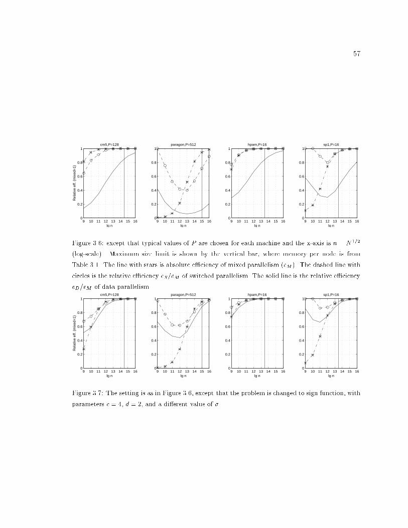
57
9 10 11 12 13 14 15 160
0.2
0.4
0.6
0.8
1cm5,P=128
lg n
Rel
ativ
e ef
f. (m
ixed
=1)
9 10 11 12 13 14 15 160
0.2
0.4
0.6
0.8
1paragon,P=512
lg n9 10 11 12 13 14 15 16
0
0.2
0.4
0.6
0.8
1hpam,P=16
lg n9 10 11 12 13 14 15 16
0
0.2
0.4
0.6
0.8
1sp1,P=16
lg n
Figure 3.6: except that typical values of P are chosen for each machine and the x-axis is n = N1=2
(log-scale). Maximum size limit is shown by the vertical bar, where memory per node is from
Table 3.1. The line with stars is absolute e�ciency of mixed parallelism (eM ). The dashed line with
circles is the relative e�ciency eS=eM of switched parallelism. The solid line is the relative e�ciency
eD=eM of data parallelism.
9 10 11 12 13 14 15 160
0.2
0.4
0.6
0.8
1cm5,P=128
lg n
Rel
ativ
e ef
f. (m
ixed
=1)
9 10 11 12 13 14 15 160
0.2
0.4
0.6
0.8
1paragon,P=512
lg n9 10 11 12 13 14 15 16
0
0.2
0.4
0.6
0.8
1hpam,P=16
lg n9 10 11 12 13 14 15 16
0
0.2
0.4
0.6
0.8
1sp1,P=16
lg n
Figure 3.7: The setting is as in Figure 3.6, except that the problem is changed to sign function, with
parameters c = 4, d = 2, and a di�erent value of �.
58
of strategy is dictated not only by �, N and P , but also the size reduction factor c and
branching degree d. This is seen in �gures 3.6 and 3.7: mixed parallelism gives less marginal
bene�t over switched or data for small values of d and large values of c (and vice versa).
Figures 3.6 and 3.7 exhibit troughs because at the lower end of problem sizes, absolute
e�ciency of all the strategies are very small but close to each other.
3.5 Experiments
Encouraged by the promising simulation and analysis, we implemented the
switched parallel scheduler as a new module in the ScaLAPACK scalable scienti�c software
library [45]. In particular, it was used to schedule the divide and conquer tree generated
by the sign function example in x3.2. The ScaLAPACK library is structured as follows.
The lowermost layer called BLACS (Basic Linear Algebra Communication Subroutines) is
built on top of a message passing layer such as NX (on the Paragon), MPI/MPL (Message
Passing Interface, on the IBM SP's), or CMMD (on the CM-5). For us BLACS provides
two types of functions:
� Routines to de�ne contexts: these are subsets of processors that form a virtual machine
and can participate in collective communication.
� Routines to transfer array sections between contexts.
On top of BLACS is built PBLAS (Parallel Basic Linear Algebra Subroutines):
these handle elementary matrix-vector and matrix-matrix operations with block-cyclic
layouts. ScaLAPACK itself is the topmost layer providing higher functionality like Cholesky
and LU factorization.
3.5.1 Software structure
Our implementation of the library has the following components.
� PBLAS/ScaLAPACK subroutines are modi�ed to export the FLOP count of relevant
subroutines symbolically in terms of the input problem size. Currently we implement
this by hand using header �les.
� The machine can be queried for its message latency and bandwidth. This is a set of
functions similar to query functions for machine epsilon and over ow.
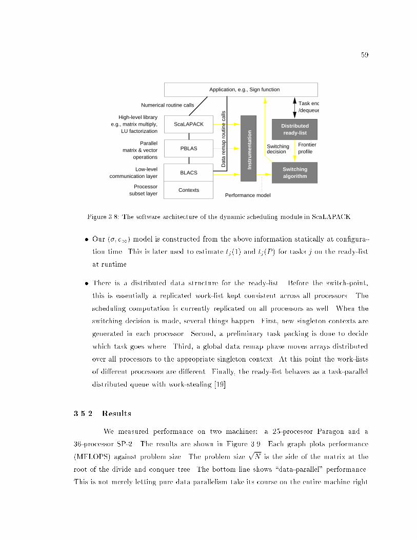
59
Low-level
ScaLAPACK
communication layer
Task enq
Application, e.g., Sign function
Processorsubset layer
LU factorization
High-level library
Contexts
Parallel
Numerical routine calls
e.g., matrix multiply,
matrix & vector
/dequeue
PBLAS
BLACS
operations
Dat
a re
map
rou
tine
calls
Inst
rum
enta
tio
n
Switchingalgorithm
Frontierprofile
Performance model
ready-listDistributed
decisionSwitching
Figure 3.8: The software architecture of the dynamic scheduling module in ScaLAPACK.
� Our (�; e1) model is constructed from the above information statically at con�gura-
tion time. This is later used to estimate tj(1) and tj(P ) for tasks j on the ready-list
at runtime.
� There is a distributed data structure for the ready-list. Before the switch-point,
this is essentially a replicated work-list kept consistent across all processors. The
scheduling computation is currently replicated on all processors as well. When the
switching decision is made, several things happen. First, new singleton contexts are
generated in each processor. Second, a preliminary task packing is done to decide
which task goes where. Third, a global data remap phase moves arrays distributed
over all processors to the appropriate singleton context. At this point the work-lists
of di�erent processors are di�erent. Finally, the ready-list behaves as a task-parallel
distributed queue with work-stealing [19].
3.5.2 Results
We measured performance on two machines: a 25-processor Paragon and a
36-processor SP-2. The results are shown in Figure 3.9. Each graph plots performance
(MFLOPS) against problem size. The problem size
pN is the side of the matrix at the
root of the divide and conquer tree. The bottom line shows \data-parallel" performance.
This is not merely letting pure data parallelism take its course on the entire machine right
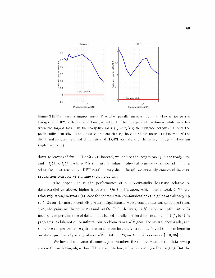
60
103
0.9
1
1.1
1.2
1.3
1.4
1.5
1.6
Sw
itche
d pa
ralle
l MF
LOP
S
Problem size: sqrt(N)
Paragon
Data parallel
103
1
1.5
2
2.5
3
Sw
itche
d pa
ralle
l MF
LOP
S
Problem size: sqrt(N)
SP2
Data parallel
Figure 3.9: Performance improvements of switched parallelism over data-parallel execution on the
Paragon and SP2, with the latter being scaled to 1. The data parallel baseline scheduler switches
when the largest task j in the ready-list has tj(1) < tj(P ); the switched scheduler applies the
pre�x-su�x heuristic. The x-axis is problem size n, the side of the matrix at the root of the
divide-and-conquer tree, and the y-axis is MFLOPS normalized to the purely data-parallel version
(higher is better).
down to leaves (of size 1�1 or 2�2). Instead, we look at the largest task j in the ready-list,and if tj(1) < tj(P ), where P is the total number of physical processors, we switch. This is
what the most reasonable HPF runtime may do, although we certainly cannot claim even
production compiler or runtime systems do this.
The upper line is the performance of our pre�x-su�x heuristic relative to
data-parallel as above; higher is better. On the Paragon, which has a weak CPU and
relatively strong network (at least for coarse-grain communication) the gains are already up
to 50%; on the more recent SP-2 with a signi�cantly worse communication to computation
cost, the gains are between 200 and 300%. In both cases, as N ! 1 no optimization is
needed; the performance of data and switched parallelism tend to the same limit (1, for this
problem). While not quite in�nite, our problem range
pN goes into several thousands, and
therefore the performance gains are much more impressive and meaningful than the bene�ts
on static problems typically of size
pN = 64 : : :128, on P = 64 processors [110, 95].
We have also measured some typical numbers for the overhead of the data remap
step in the switching algorithm. They are quite low; a few percent. See Figure 3.10. But the
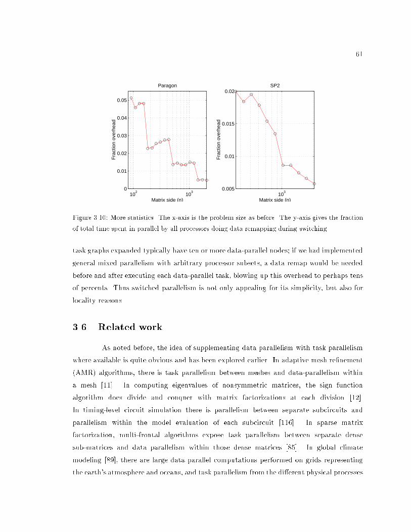
61
103
0.005
0.01
0.015
0.02
Matrix side (n)
Fra
ctio
n ov
erhe
ad
SP2
102
103
0
0.01
0.02
0.03
0.04
0.05
Matrix side (n)
Fra
ctio
n ov
erhe
ad
Paragon
Figure 3.10: More statistics. The x-axis is the problem size as before. The y-axis gives the fraction
of total time spent in parallel by all processors doing data remapping during switching.
task graphs expanded typically have ten or more data-parallel nodes; if we had implemented
general mixed parallelism with arbitrary processor subsets, a data remap would be needed
before and after executing each data-parallel task, blowing up this overhead to perhaps tens
of percents. Thus switched parallelism is not only appealing for its simplicity, but also for
locality reasons.
3.6 Related work
As noted before, the idea of supplementing data parallelism with task parallelism
where available is quite obvious and has been explored earlier. In adaptive mesh re�nement
(AMR) algorithms, there is task parallelism between meshes and data-parallelism within
a mesh [11]. In computing eigenvalues of nonsymmetric matrices, the sign function
algorithm does divide and conquer with matrix factorizations at each division [12].
In timing-level circuit simulation there is parallelism between separate subcircuits and
parallelism within the model evaluation of each subcircuit [116]. In sparse matrix
factorization, multi-frontal algorithms expose task parallelism between separate dense
sub-matrices and data parallelism within those dense matrices [85]. In global climate
modeling [89], there are large data parallel computations performed on grids representing
the earth's atmosphere and oceans, and task parallelism from the di�erent physical processes
62
being modeled.
Several researchers have proposed support to take advantage of this mixed
parallelism. In the theory area, the best known on-line scheduling algorithm for mixed
parallelism is 2:62-optimal [16, 52], and the best o�-line algorithm is 2-optimal [113, 87].
But these are worst-case guarantees. In the systems area, the Paradigm compiler [95],
iWarp compiler [110], and NESL compiler [32] all support forms of mixed task and data
parallelism, and there are plans to merge data Fortran D with Fortran M [56] and pC++
with CC++ [84] to support mixed parallelism. The compiler e�orts all depend on static
task graph and pro�le data and perform extensive optimizations to allocate processors. We
have already noted how dynamic task parallelism is more promising to exploit.
A problem domain quite di�erent from scienti�c computing where mixed paral-
lelism has been used is in parallel database query scheduling. In a relational database, each
query is roughly speaking an in-tree of parallelizable tasks; where each task is an operator
like a join or select. Each operator has partitioned parallelism similar to data-parallelism.
A chain of operators may also show pipelined parallelism, but we can regard those nodes to
be collapsed into a single node with data parallelism. There is also task parallelism between
unordered nodes. Recently algorithms have been designed for trading between locality and
load balance in this scenario [33]. We will come back to similar problems in Chapter 4.
The switching technique has been independently discovered after our paper [26]
was published in a di�erent context: that of scheduling tasks with penalties. Every task
has a running time, and a penalty for rejection; the goal is to minimize the sum of the
makespan of accepted tasks and the penalty of rejected tasks [15]. While their main result
is an on-line algorithm for independent tasks, we also give an o�-line algorithm for trees
(this can be generalized to series-parallel graphs).
3.7 Discussion
We have shown in this chapter that by exploiting dynamic task parallel to
supplement the diminishing returns of data parallelism in mixed parallel divide-and-conquer
applications, and by designing simple heuristics for switched scheduling, signi�cant
performance improvements are possible. We conclude the chapter with a few comments.
What happens if the leaf tasks are di�erent from the interior tasks? It is usually the
case that the leaf tasks are more e�cient in terms of CPU operations, but they may be less
63
parallelizable. This in fact happens in the non-symmetric eigenvalue code. The pre�x-su�x
heuristic can be modi�ed so that the task packing is done with the leaf estimates. This
works well in practice (the pro�t margin is even higher than 300%), but is not interesting
to report on from the modeling and analysis point of view.
What happens if the task tree folds back, as in a conquer phase? In our application
domain, the sizes are known during the unfolding, so the folding back will be a static
scheduling problem. In terms of the runtime strategy, processors can do one of these two
things:
� rendezvous at the �rst phase switch point, compute the second phase reverse switch
frontier, and go into a task parallel phase in between, OR
� go into the �rst phase task parallel mode as before, rendezvous before the folding
back, compute the reverse switch frontier, and proceed as above.
Can we extend the analysis to make global statements about the switching
heuristic, in particular, qualify the empirical intuition that since problem sizes decrease
down any path, a switching decision cannot be far wrong? This will depend on the
out-degree and the size shrink factor.
What if data transfer cost at the switching point/s are signi�cant? This will be
particularly important for arbitrary task graphs with arbitrary problem sizes at the nodes,
where many switches may be needed. In that case we will need to minimize number or cost
of switches, or trade that against the costs of data parallel ine�ciency and task parallel
packing loss.
64
Chapter 4
Scheduling resource constrained
jobs
4.1 Introduction
So far in this thesis we have been concerned mostly with optimizing the
performance of a single parallel program. On a typical multiprocessing system several
such programs run simultaneously, contending for CPU time and other resources. While
classical scheduling theory has been largely concerned with processor scheduling, memory,
network and IO bandwidth are other resources which dictate how best to schedule programs
with diverse needs. Moreover, classical scheduling results are predominantly for minimizing
makespan (the �nish time of a �xed set of programs); in real life, system utilization, fairness,
and honoring priority are also important. In this chapter we will develop new techniques
for scheduling such workloads.
To use terminology consistent with scheduling literature, we will refer to what
independent users submit as programs. Each program is a collection of jobs. (In Chapter 3
there was only one program, and we called the jobs parallelizable or data-parallel tasks.)
Every job speci�es some resources that it needs to reserve during execution and perhaps
some other jobs that need to �nish before it can start.
Judicious job scheduling is crucial to obtaining fast response and e�ective
utilization. Consequently, algorithms for scheduling have been extensively researched since
the 60's, both in theory and in practice. In the past decade, there has been increasing
65
interest in scheduling speci�cally for parallel systems. There is increased awareness of
general resource scheduling problems, rather than just processor scheduling [50].
Owing to the vastly di�erent nature and applicability of sequential and parallel
computing systems, the scheduling problems of practical interest are rather di�erent in the
two settings. For example, scheduling general-purpose jobs is essential for a uniprocessor
operating systems, while it is hardly an issue yet for existing parallel systems, none of which
run the average workstation workload; similarly, scheduling threads for massive game tree
searches is a reality for parallel systems while it is not an issue for uniprocessors.
In this chapter, we extend our scope from optimizing single programs using
compiler and runtime approaches to that of scheduling multi-user parallel workloads. To
propose a model, we focus on applications where parallelism has been e�ectively exploited.
We isolate parallel databases and scienti�c computing as two such areas. In both these areas
the computation is well-structured so regular subproblems can be solved in parallel, and
the resource requirements of jobs can be estimated in advance. For these reasons, parallel
computing has proven highly successful in these two areas. Here, we carefully model the
resource scheduling problems in these applications and study them.
In the model we abstract from these applications, many users submit programs to
the system over time; each program is a directed acyclic graph of jobs; the graph is assumed
to be known when the program is submitted. A job is characterized by a set of resource
requirements, which are also known at submission time. Resources are of various di�erent
types. Some resources, like processors, can be traded for time gracefully, while others,
like memory, are not exible in such a continuous fashion. The acyclic graph represents
precedence constraints; each job speci�es a set of predecessors that must complete before it
starts.
We initiate a study of such resource scheduling models. Two features distinguish
our goal from many classical results. First, our jobs are themselves parallelizable, like the
data-parallel tasks in the applications in Chapter 3. Second, rather than minimizing the
�nish time of a �xed set of jobs, we wish to accept programs over time; these programs
have priorities and we minimize the sum of �nish time weighted by the respective priorities
(this is called a minsum metric, as compared to makespan, which is a minmax metric). The
results in this chapter represent initial work towards extending scheduling algorithms to
take into account features of real-life multiprocessing workload, and we expect a number of
possible directions for extending them.
66
4.1.1 Model and problem statement
We describe some motivating scenarios in parallel databases and scienti�c compu-
tation later in x4.2. The model and problems we abstract from there are as follows.
Model. The multiprocessor consists of m identical processors and s types of other
resources not including the processors. It is not necessary to maintain the identity of
programs separate from jobs: the arrival of a program is equivalent to the arrival of some
number of jobs, specifying some precedence graph between them. Thus we will consider the
unit of computation to be a job. A job j will need several kinds of resources. A resource is
malleable if there is a range of trade-o�s between the amount of that resource allocated to
the job and its running time. It is non-malleable if the job has to reserve a �xed amount of
the resource for as long as it runs, no matter what that time is.
A job arrives with the following information:
� The trade-o� between processor and time. This is expressed by a running time
function, tj(�), on 1 � � � m processors, where m is the number of processors
in the system. In general, the running time tj would be a function of all malleable
resources. Our case studies seem to indicate that only one resource is really malleable:
processors. Once the processor allocation is �xed, we shall see that all other resouces
essentially become non-malleable.
We shall study various forms of the trade-o� function. In the most general setting
we will assume that tj( ) are arbitrary computable functions; in this case we say the
processor resource is malleable. In a simpler setting, we will assume tj(�) = tjmj=�,
where j shows linear speedup up to mj processors, on which its running time is tj ;
in this case we shall say the processor resource is perfectly malleable, up to a limit.
Some programs are not written to be adaptive to any number of processors. For jobs
generated by such programs, processors are a non-malleable resource. Job j will run
on exactly mj processors for time tj . We will round tj 's to powers of 2 for convenience,
and also denote T = maxjftjg=minjftjg. We will overload tj to represent both a �xed
number and a function; the meaning will be clear from context.
� Precedence constraints: a set of jobs (that have already been submitted to the
scheduler) that must complete before j can start. This induces a partial order �
67
on the jobs. Note that if jobs arrive on-line, then � may be revealed to the scheduler
gradually.
� Apart from the processors requirement, jobs may also specify a vector of other
non-malleable resources. We will let there be s distinct types of resources, where we
can assume s = O(1). E.g., if we are modeling processors, memory and IO bandwidth
as resources, s = 2. The resource vector will be denoted ~rj = (rj1; : : : ; rjk; : : : ; rjs), of
the fractions rjk of resource of type k demanded by job j, k = 1; : : : ; s. For notational
simplicity we scale the total available resource to be 1 unit for each type. For the
reasons above we keep the processor resource separate from all others.
� Job j speci�es a positive priority wj, also called its weight. The higher this number,
the more pro�table it is to �nish it early.
Problem. A scheduler is an algorithm that speci�es for each processor and time slot,
a portion of at most one job to be executed, so that all jobs get executed subject to all
the constraints above. Consider a set of n jobs. Let a scheduler complete job j at time
Cj . The two performance metrics that we seek to minimize are the makespan, maxj Cj
and the weighted average completion time (WACT),1n
Pj wjCj . Other possible metrics are
mentioned in x4.6, some of those are provably much harder than either makespan or WACT.
We impose further constraints on the schedulers. First, preemption is not allowed.
Time-slicing and preemption of space-shared resources is very expensive because (1) the
state has to be evicted to slower layers of the memory hierarchy, (2) processes have to
synchronize and switch across protection domains, and (3) in- ight messages have to be
ushed and reinjected [50, page 6]. Anecdotal evidence suggests that many practitioners
switch o� time sharing for production runs on parallel machines that do not permit creating
dedicated space partitions. To recover from pathological cases, some machines (like the
Cray T3D) have an expensive roll-in/out mechanism, but it is important to minimize its
deployment. Second, the number of types of non-malleable resources, s, can be assumed to
be a small constant. Resources are not private to processors; they are equally accessible
by all jobs. Typically the set of resources will be memory, disk and network bandwidth
(i.e., s = 3). IO and network bandwidth are often centralized from the user's perspective.
With respect to memory, our model is closer to SMP's than distributed memory machines.
Third, it su�ces for our scheduler to be a sequential algorithm since in both databases and
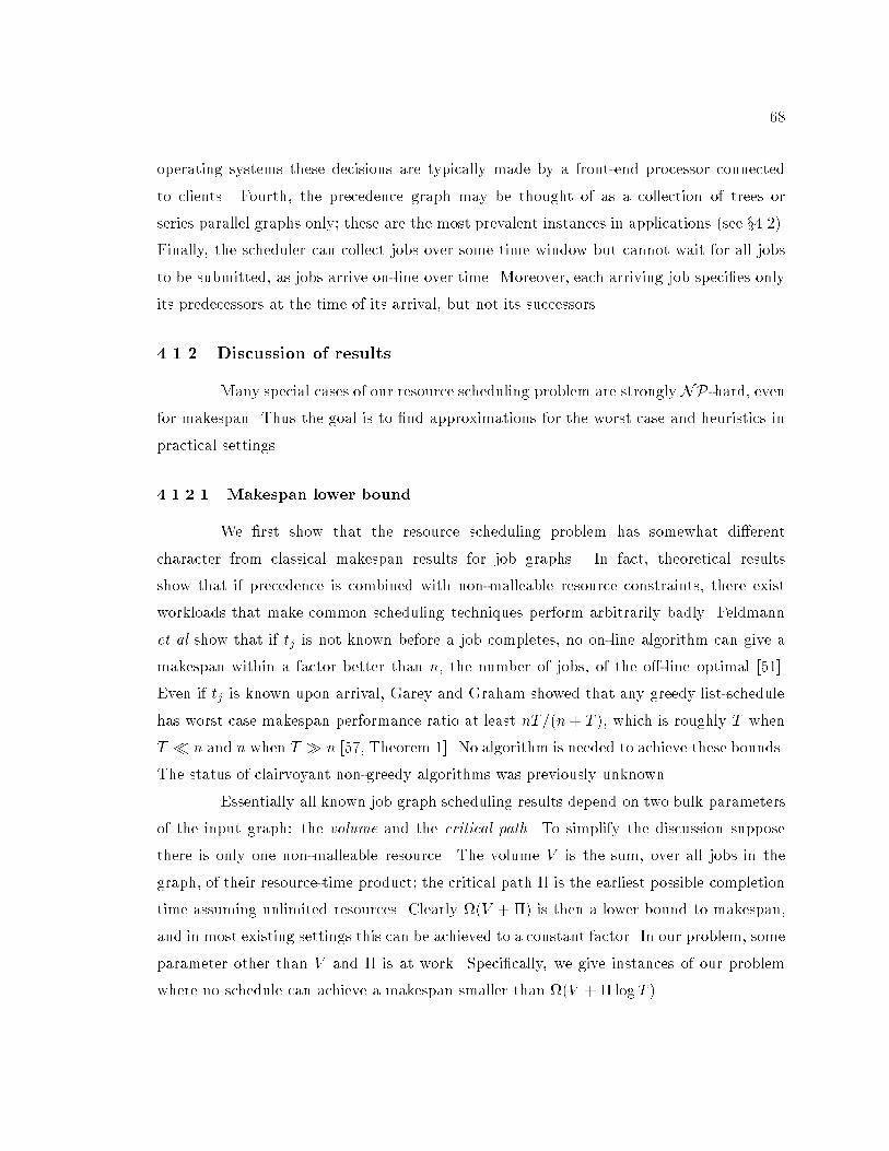
68
operating systems these decisions are typically made by a front-end processor connected
to clients. Fourth, the precedence graph may be thought of as a collection of trees or
series parallel graphs only; these are the most prevalent instances in applications (see x4.2).Finally, the scheduler can collect jobs over some time window but cannot wait for all jobs
to be submitted, as jobs arrive on-line over time. Moreover, each arriving job speci�es only
its predecessors at the time of its arrival, but not its successors.
4.1.2 Discussion of results
Many special cases of our resource scheduling problem are strongly NP-hard, evenfor makespan. Thus the goal is to �nd approximations for the worst case and heuristics in
practical settings.
4.1.2.1 Makespan lower bound
We �rst show that the resource scheduling problem has somewhat di�erent
character from classical makespan results for job graphs. In fact, theoretical results
show that if precedence is combined with non-malleable resource constraints, there exist
workloads that make common scheduling techniques perform arbitrarily badly. Feldmann
et al show that if tj is not known before a job completes, no on-line algorithm can give a
makespan within a factor better than n, the number of jobs, of the o�-line optimal [51].
Even if tj is known upon arrival, Garey and Graham showed that any greedy list-schedule
has worst case makespan performance ratio at least nT=(n+ T ), which is roughly T when
T � n and n when T � n [57, Theorem 1]. No algorithm is needed to achieve these bounds.
The status of clairvoyant non-greedy algorithms was previously unknown.
Essentially all known job graph scheduling results depend on two bulk parameters
of the input graph: the volume and the critical path. To simplify the discussion suppose
there is only one non-malleable resource. The volume V is the sum, over all jobs in the
graph, of their resource-time product; the critical path � is the earliest possible completion
time assuming unlimited resources. Clearly (V + �) is then a lower bound to makespan,
and in most existing settings this can be achieved to a constant factor. In our problem, some
parameter other than V and � is at work. Speci�cally, we give instances of our problem
where no schedule can achieve a makespan smaller than (V + � logT ).
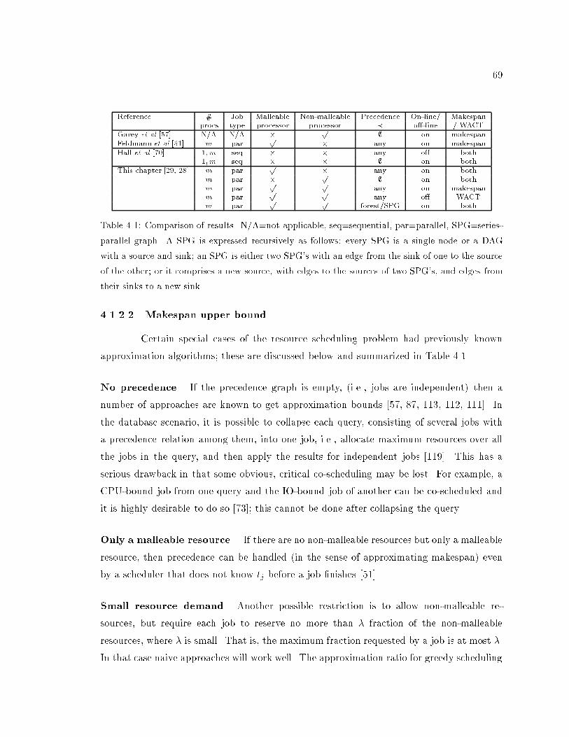
69
Reference # Job Malleable Non-malleable Precedence On-line/ Makespanprocs type processor processor � o�-line / WACT
Garey et al [57] N/A N/A � p ; on makespan
Feldmann et al [51] m parp � any on makespan
Hall et al [70] 1;m seq � � any o� both1;m seq � � ; on both
This chapter [29, 28] m parp � any on both
m par � p ; on bothm par
p pany on makespan
m parp p
any o� WACTm par
p pforest/SPG on both
Table 4.1: Comparison of results. N/A=not applicable, seq=sequential, par=parallel, SPG=series-
parallel graph. A SPG is expressed recursively as follows: every SPG is a single node or a DAG
with a source and sink; an SPG is either two SPG's with an edge from the sink of one to the source
of the other; or it comprises a new source, with edges to the sources of two SPG's, and edges from
their sinks to a new sink.
4.1.2.2 Makespan upper bound
Certain special cases of the resource scheduling problem had previously known
approximation algorithms; these are discussed below and summarized in Table 4.1.
No precedence. If the precedence graph is empty, (i.e., jobs are independent) then a
number of approaches are known to get approximation bounds [57, 87, 113, 112, 111]. In
the database scenario, it is possible to collapse each query, consisting of several jobs with
a precedence relation among them, into one job, i.e., allocate maximum resources over all
the jobs in the query, and then apply the results for independent jobs [119]. This has a
serious drawback in that some obvious, critical co-scheduling may be lost. For example, a
CPU-bound job from one query and the IO-bound job of another can be co-scheduled and
it is highly desirable to do so [73]; this cannot be done after collapsing the query.
Only a malleable resource. If there are no non-malleable resources but only a malleable
resource, then precedence can be handled (in the sense of approximating makespan) even
by a scheduler that does not know tj before a job �nishes [51].
Small resource demand. Another possible restriction is to allow non-malleable re-
sources, but require each job to reserve no more than � fraction of the non-malleable
resources, where � is small. That is, the maximum fraction requested by a job is at most �.
In that case naive approaches will work well. The approximation ratio for greedy scheduling
70
can be easily shown to be 1+1
1�� . This is however useless even if one, or a few jobs need a
large fraction, or equivalently, if � approaches 1. In fact, � = 1�O(1=m) su�ces to render
the greedy schedule useless. Intuitively, a few resource-intensive jobs can delay a convoy of
tiny jobs.
We show that we can attain the existential lower bound on the makespan, for the
above choice of parameters (V , � and T ). We give a simple approximation algorithm that
matches the O(V + � logT ) makespan bound. In contrast to our algorithm, most known
practical solutions use some variant of greedy list- or queue-type scheduling [50, 59, 90].
Jobs on arrival are placed in a list ordered by some heuristic (often FIFO). The scheduler
dispatches the �rst ready job on the list when enough resources become available. List
scheduling and its variants are appealingly simple to implement, but they can be notoriously
bad, which is not surprising given the negative results mentioned above.
4.1.2.3 Weighted average completion time
We extend the makespan upper bound to the weighted average completion time
metric. For this we use a recent elegant framework by Hall et al for optimizing WACT, which
we also show to be nearly optimal for makespan. The framework needs two subroutines: a
knapsack-type routine for picking a set of \high-returns" jobs to run next, and a makespan
algorithm to run them. By designing these subroutines, we give the �rst logarithmic
approximation algorithm for our resource scheduling problem using the WACT metric.
For several slightly simpler variants, the logarithmic factor can be reduced to a small
constant. Many of these on-line results are the �rst constant approximation algorithms for
the corresponding problems, on-line or o�-line, while others are on-line algorithms whose
performance is close to the best known o�-line results. These ideas can be adapted to yield
the �rst known (o�-line or on-line) constant-approximation algorithms for minsum open
shop scheduling and minsum job shop scheduling with a �xed number of machines.
Previous work on the WACT metric gave either non-clairvoyant, preemptive
solutions for sequential jobs or jobs that used a perfectly malleable processor resource,
with job precedence [41]; or clairvoyant, non-preemptive solutions for independent jobs
with only non-malleable resource, if any [92, 112]. Apart from algorithm design, we believe
it is important to point out some di�erences between existing scheduling literature and
features needed by schedulers in parallel computing systems. We also remark that although
71
our problem is di�erent from existing theoretical settings, our solution borrows from various
existing techniques [57, 103, 29, 70].
In x4.2 we study database and scienti�c computing scenarios to justify our model.In x4.3 and x4.4 we give the makespan lower and upper bounds. In x4.5 we show how to
extend the makespan algorithm to a WACT algorithm. In x4.6 we pose some unresolved
problems.
4.2 Motivation
4.2.1 Databases
Query scheduling in parallel databases is a topic of active research [23, 90, 119, 66,
59]. Queries arrive from many users to a front-end manager process. A query is an in-tree,
where the internal vertices are operations like sort, merge, select, join etc., which we call
jobs. (We think of pipelines as collapsed into single vertices.) The leaves are relations
stored on disk. Edges represent data transfer; the source vertex sends output to disk, which
the target vertex later reads. Queries may have a priority associated with them, e.g., an
interactive transaction has high priority and statistics collection has low priority.
Databases keep certain access statistics along with the relations, which are used
to predict the size of the result of a join or a select and how many CPU instructions will
be required to compute these results. The tools are standard in database literature [101].
For parallel databases, one can also estimate for each operation the maximum number
of processors that can be employed for near-linear speedup [73]. Thus tj and mj can be
estimated when a job arrives. Estimates of sizes of intermediate results can be used to
estimate the memory and disk bandwidth resource vector ~rj .
The running time of a job is roughly inversely proportional to the number of
processors in the range [1; mj], but not the total available memory. For example, a
hash-join between two relations R1 and R2 with, say, R1 being smaller, takes time roughly
proportional to dlogr jR1je, where r is the memory allocated; typically the query planner
picks r = jR1j or r = jR1j1=2, independent of other queries [90]. Once processor and memoryallocation are �xed, the disk bandwidth requirement can be estimated from the total IO
volume and job running time.
This model is best suited to shared memory databases running on symmetric
72
multiprocessors (SMP) with shared access to disk [73]. They currently scale to 30{40
processors. There is growing consensus that SMP's and scalable multiprocessors will
converge to networked clusters of SMP nodes [66]. Since communication costs across clusters
is much more expensive than shared access within a cluster, the expectation is that most
queries will be parallelized within an SMP node.
4.2.2 Scienti�c applications
Multiprocessor installations are shared by many users submitting programs to
manager processes running on the front-end that schedules them. Examples of front-end
schedulers are DJM (distributed job manager) on the CM5, NQS (network queuing system)
on the Paragon, POE (parallel operating environment) on the SP2. Users may submit a
script to the manager. A script �le has a sequence of invocations of executables, each line
typically specifying a priority, the number of processors, estimated memory and running
time. Notice that although there may be some exibility in the amount of memory needed,
the user typically speci�es a �xed choice to the scheduler, which has to regard it as in exible.
To improve utilization, system support has been designed to express jobs at a �ner level
inside an application and convey the information to the resource manager by annotating
the parallel executable [65, 48, 91].
The common precedence graphs are chains for scripts, series-parallel graphs
(de�ned in Table 4.1) for structured programs, forests for database queries, and trees for
divide-and-conquer and branch-and-bound algorithms.
4.2.3 Fidelity
The most general representation of a job is its running time as a function of the
resources allocated to it. It is di�cult to �nd this function [59], and unclear if it is simple
enough to be used by the optimizer. We group the resources into two types: malleable and
non-malleable. We handle only one malleable resource that a�ects the running time. It
may be of interest to evaluate more elaborate alternatives. We assume that tj is known
(constant or function), which is reasonable for our target domain, but for less predictable
applications, some type of adaptive scheduling is needed. Even though virtual memory
appears to make memory a malleable resource, most parallel systems that support paging
(including the SP2 or the Paragon, and excluding the CM5) strongly encourage users to
73
write programs that �t in physical memory. Paging non-cooperatively on a multiprocessor
can be disastrous for performance.
We have tried to avoid both unwarranted simpli�cations and gratuitous generality.
For example, we have not assumed for simplicity that all resources are malleable. Memory is
clearly not malleable, even for programs that are adaptive in limited ways to the amount of
allocated memory. On the other hand, we have not modeled the details of the inter-processor
network.
4.3 Makespan lower bound
Many results in DAG scheduling rely on two bulk parameters of the workload.
One, which we call the volume parameter, is the sum of resource-time products over jobs in
the graph, denoted V . For example, consider jobs with only one resource type: processors.
If each job runs on only one processor, as in list-scheduling [64], then the fractional resource
every job occupies is rj = 1=m, where there are m processors in all. If the processor
resource is perfectly malleable up to limit mj , or non-malleable, �xed at mj for job j, then
the fractional resource job j occupies is rj = mj=m. In all cases we de�ne V =
Pj tjrj.
The other parameter is the critical path � of the graph. � = maxj �j , where �j is the
minimum time at which j can complete, if in�nite resources were available.
(V +�) is a lower bound to makespan. If the problem is relaxed to remove either
precedence or non-malleable resources, then this lower bound can be achieved to a constant
factor: �+1m
Pjtj = �+V for sequential jobs [64], and �+(
p5�1
3�p5)1m
Pjtjmj = �+O(V )
for malleable jobs [51]. These depend on arguments of the form: \if a critical path is being
ignored, most of the resources are being utilized."
In this section, we show that O(V +�) makespan is not always possible with both
non-malleable resources and precedence constraints. Thus this di�erentiates our problem
from list-scheduling [64, 57] and malleable job scheduling [51]. Our formulation is di�erent
in avor because jobs may have to wait even when resource utilization is very low because
their speci�c requirement of the non-malleable resources are not met. In contrast, jobs can
proceed with a smaller amount of a malleable resource with proportionate slowdown. Thus
some parameter other than V and � is at work.
Claim 4.3.1 With precedence and non-malleable resources, the optimal makespan can be
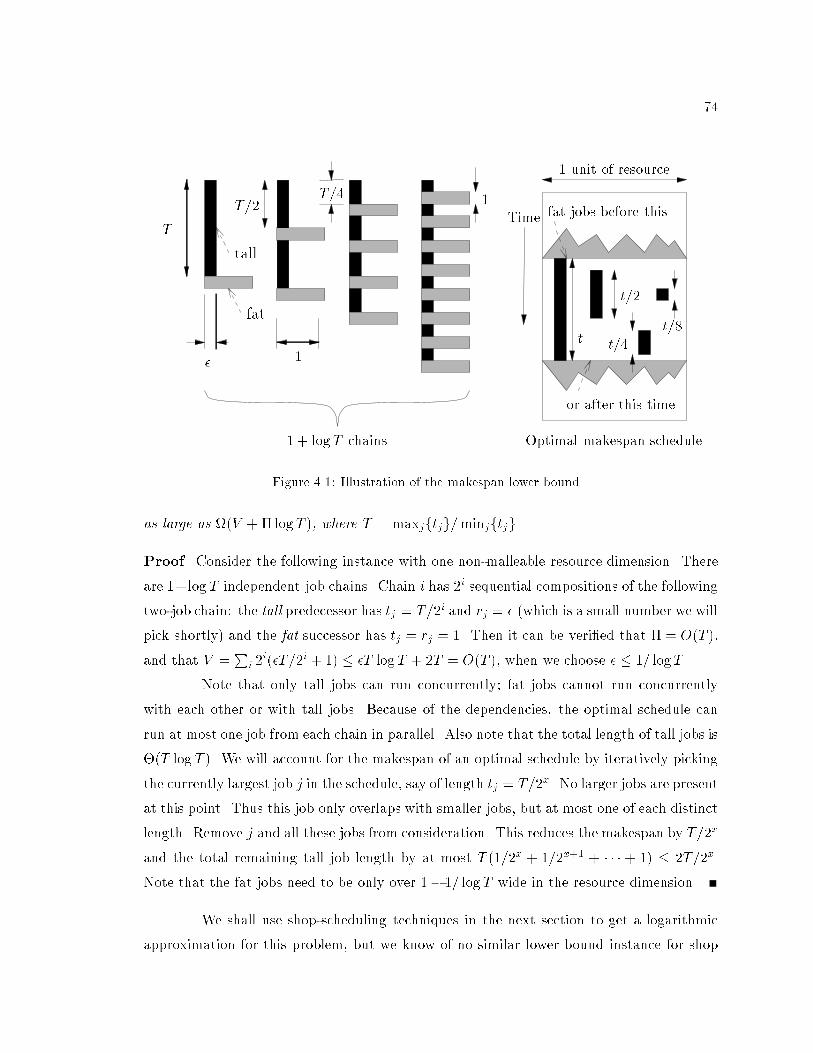
74
fat jobs before this...Time
� 1
T
T=2T=4
1
1 + logT chains
1 unit of resource
Optimal makespan schedule
t=2
t=4t
tall
fatt=8
... or after this time
Figure 4.1: Illustration of the makespan lower bound.
as large as (V + � logT ), where T = maxjftjg=minjftjg.
Proof. Consider the following instance with one non-malleable resource dimension. There
are 1+log T independent job chains. Chain i has 2i sequential compositions of the following
two-job chain: the tall predecessor has tj = T=2i and rj = � (which is a small number we will
pick shortly) and the fat successor has tj = rj = 1. Then it can be veri�ed that � = O(T ),
and that V =
Pi 2
i(�T=2i + 1) � �T logT + 2T = O(T ), when we choose � � 1= logT .
Note that only tall jobs can run concurrently; fat jobs cannot run concurrently
with each other or with tall jobs. Because of the dependencies, the optimal schedule can
run at most one job from each chain in parallel. Also note that the total length of tall jobs is
�(T log T ). We will account for the makespan of an optimal schedule by iteratively picking
the currently largest job j in the schedule, say of length tj = T=2x. No larger jobs are present
at this point. Thus this job only overlaps with smaller jobs, but at most one of each distinct
length. Remove j and all these jobs from consideration. This reduces the makespan by T=2x
and the total remaining tall job length by at most T (1=2x + 1=2x+1 + � � � + 1) � 2T=2x.
Note that the fat jobs need to be only over 1� 1= logT wide in the resource dimension.
We shall use shop-scheduling techniques in the next section to get a logarithmic
approximation for this problem, but we know of no similar lower bound instance for shop
75
problems. Speci�cally, a shop problem instance has some number of jobs; each job j consists
of some operations; the i-th operation must run for time tji on a speci�ed machine mji;
for each job, no two of its operations may run concurrently. Let � = maxjfP
itjig and
V = maxmfP
mji=mtjig, then maxf�; V g is the only known lower bound on the shop
makespan based on bulk properties of the instance; this seems to indicate that the resource
scheduling problem is somewhat di�erent from shop-scheduling.
Claim 4.3.1 also implies that a recent elegant constant factor WACT approximation
technique due to Chekuri et al, which converts uniprocessor schedules to multiprocessor
schedules [34], will not generalize to handle non-malleable resources. Their technique is
to start with a uniprocessor schedule, where job j completes at time C1j, and derive an
m-machine schedule with Cm
j= O(C1
j=m+�j). In their model all jobs are sequential and
the jobs need no other resources. If we additionally add jobs that request non-malleable
resources, their conversion does not go through, and with good reason: if it did, a schedule
with O(�) additive term, rather than the (� logT ) term that we showed above, will hold,
thus violating the lower bound.
4.4 Makespan upper bound
In this section we will give an algorithm Makespan that is polynomial in s, T and
n that will achieve a makespan of O(V s+� logT ) for an input set of jobs J with the bulk
parameters V , � and T de�ned before, where there is one malleable resource and there are
s types of non-malleable resources. Let ~vj = tj~rj, and V = maxf 1m
Pjmjtj ; k
Pj~vjk1g.
Also let �j be the critical path length from a root through job j, and � = maxjf�jg.The makespan algorithm �rst invokes the malleable scheduling of Feldmann et
al [51] to allocate processors to jobs in J , and to assign (infeasible) preliminary execution
intervals to these jobs that still violate other resource constraints. Then we partition the
jobs into a sequence of layers with jobs within a layer being independent of each other.
Finally we schedule these layers one by one using bin-packing.
Step 1. Let12 < < 1 be a free parameter to be set later. Compute a greedy schedule for
J ignoring all non-malleable resource requirements, as follows. Whenever there are more
than m free processors, schedule any job j in J (whose predecessors have all completed)
on the minimum of mj and the number of free processors [51].
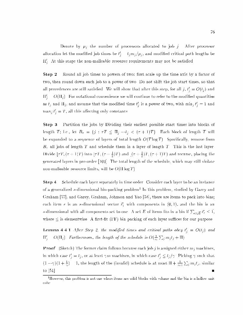
76
Denote by �j the number of processors allocated to job j. After processor
allocation let the modi�ed job times be t0j= tjmj=�j , and modi�ed critical path lengths be
�0j. At this stage the non-malleable resource requirements may not be satis�ed.
Step 2. Round all job times to powers of two: �rst scale up the time axis by a factor of
two, then round down each job to a power of two. Do not shift the job start times, so that
all precedences are still satis�ed. We will show that after this step, for all j, t0j= O(tj) and
�0j= O(�j). For notational convenience we will continue to refer to the modi�ed quantities
as tj and �j , and assume that the modi�ed time t0jis a power of two, with minj t
0j= 1 and
maxj t0j= T , all this a�ecting only constants.
Step 3. Partition the jobs by Dividing their earliest possible start times into blocks of
length T ; i.e., let B� = fj : �T � �j � tj < (� + 1)Tg. Each block of length T will
be expanded to a sequence of layers of total length O(T logT ). Speci�cally, remove from
B� all jobs of length T and schedule them in a layer of length T . This is the last layer.
Divide [�T; (� + 1)T ) into [�T; (� + 12)T ) and [(� + 1
2)T; (� + 1)T ) and recurse, placing the
generated layers in pre-order [103]. The total length of the schedule, which may still violate
non-malleable resource limits, will be O(� logT ).
Step 4. Schedule each layer separately in time order. Consider each layer to be an instance
of a generalized s-dimensional bin-packing problem1In this problem, studied by Garey and
Graham [57], and Garey, Graham, Johnson and Yao [58], there are items to pack into bins;
each item e is an s-dimensional vector ~re with components in (0; 1), and the bin is an
s-dimensional with all components set to one. A set E of items �ts in a bin if
Pe2E ~re � ~1,
where � is elementwise. A �rst-�t (FF) bin packing of each layer su�ces for our purpose.
Lemma 4.4.1 After Step 2, the modi�ed times and critical paths obey t0j= O(tj) and
�0j= O(�j). Furthermore, the length of the schedule is O( 1
m
Pj mjtj + �).
Proof. (Sketch) The former claim follows because each job j is assigned eithermj machines,
in which case t0j= tj , or at least m machines, in which case t0
j� tj= . Picking such that
(1� )(1+ 1 ) = 1, the length of the (invalid) schedule is at most � +
1m
Pj mjtj , similar
to [51].
1However, this problem is not one where items are solid blocks with volume and the bin is a hollow unitcube.
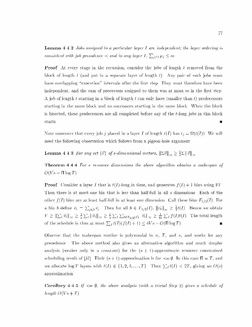
77
Lemma 4.4.2 Jobs assigned to a particular layer I are independent; the layer ordering is
consistent with job precedence � and in any layer I,P
j2I �j � m.
Proof. At every stage in the recursion, consider the jobs of length t removed from the
block of length t (and put in a separate layer of length t). Any pair of such jobs must
have overlapping \execution" intervals after the �rst step. They must therefore have been
independent, and the sum of processors assigned to them was at most m in the �rst step.
A job of length t starting in a block of length t can only have (smaller than t) predecessors
starting in the same block and no successors starting in the same block. When the block
is bisected, these predecessors are all completed before any of the t-long jobs in this block
starts.
Note moreover that every job j placed in a layer I of length t(I) has tj = (t(I)). We will
need the following observation which follows from a pigeon-hole argument.
Lemma 4.4.3 For any set f~vg of s-dimensional vectors, k�~vk1 � 1s� k~vk1.
Theorem 4.4.4 For s resource dimensions the above algorithm obtains a makespan of
O(V s +� logT ).
Proof. Consider a layer I that is t(I)-long in time, and generates f(I) + 1 bins using FF.
Then there is at most one bin that is less than half-full in all s dimensions. Each of the
other f(I) bins are at least half-full in at least one dimension. Call these bins F1=2(I). For
a bin b de�ne ~vb =P
j2b ~vj . Then for all b 2 F1=2(I), k~vbk1 � 14 t(I). Hence we obtain
V � kPb ~vbk1 � 1s
Pb k~vbk1 � 1
s
PI
Pb2F1=2(I) k~vbk1 � 1
4s
PI f(I)t(I). The total length
of the schedule is thus at most
PIt(I)(f(I) + 1) � 4V s+ O(� logT ).
Observe that the makespan routine is polynomial in n, T , and s, and works for any
precedence. The above method also gives an alternative algorithm and much simpler
analysis (weaker only in a constant) for the (s + 1)-approximate resource constrained
scheduling result of [57]. Their (s+ 1)-approximation is for �= ;. In this case � = T , and
we allocate logT layers with t(I) 2 f1; 2; 4; : : : ; Tg. Then
PI t(I) < 2T , giving an O(s)
approximation.
Corollary 4.4.5 If �= ;, the above analysis (with a trivial Step 3) gives a schedule of
length O(V s+ T ).
78
We do not know the status of the gap between the upper and lower bound w.r.t. the
factor of s.
4.5 Weighted average completion time
In this section we will describe how to extend the makespan algorithm developed
earlier to the weighted average completion time (WACT) metric. We �rst justify why this
metric is of interest. Makespan algorithms were designed for batch operations, which means
that only the maximum completion time maxjfCjg was of concern. In parallel computer
installations, jobs are submitted by di�erent parties over time, are collected over some
windows and then scheduled with some priorities. One good metric is response time, which
over an arbitrary set of test jobs can be denoted
Pj(Cj � aj), where aj is when job j is
submitted and Cj is the completion time. Unfortunately this is a rather intractable metric
in the worst case, but in practice the following strategy works well: collect jobs in suitable
time windows, assign priorities to jobs based on how long they have been waiting, and
then run a priority-based batch scheduling algorithm to select which jobs to do next. The
Operating Systems research literature has many proposals for choosing the priority function
to favor starved or short jobs [54].
We will thus be interested in designing subroutines that input a set of jobs that
have arrived but not been scheduled yet, and constructs a schedule with near-minimalPjwjCj , where wj is the priority assigned to job j and Cj the completion time of job j
measured from the current time. This metric is called weighted average completion time
(WACT). For a single processor and no other resources, \shortest remaining processing
time" is optimal for WACT, given independent jobs. In some sense, we show how to
generalize this intuition to multiple processors, multiple resource types, and jobs with
precedence.
4.5.1 The bicriteria framework
For a single processor, any optimal WACT schedule has optimal makespan.
Surprisingly, this does not hold for unrelated parallel machines, on which a job can run
at various speeds on various machines, and the speed of a machine is not independent of
the job. For unrelated machines, there are instances where any optimal WACT schedule
for n jobs has makespan (logn= log logn) times the optimal makespan [74].
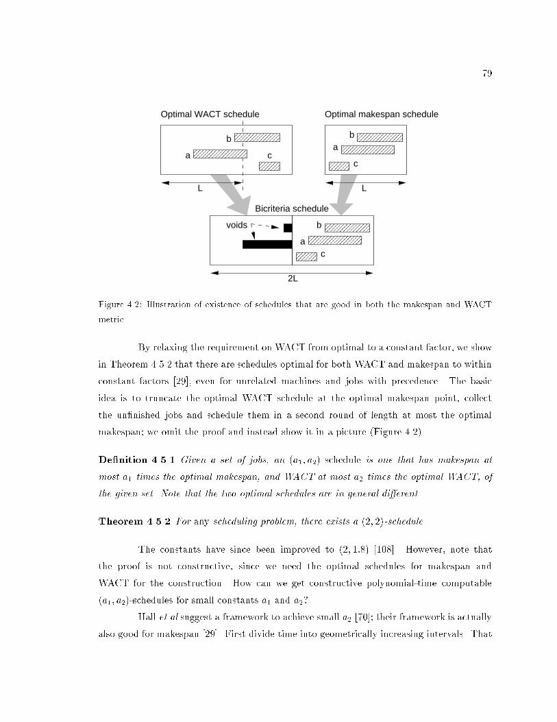
79
2L
voids
����������
������ ������������������������������
������������������
������������
Optimal WACT schedule Optimal makespan schedule
L L
Bicriteria schedule
��������a
b
c
ba
c
b
ac
Figure 4.2: Illustration of existence of schedules that are good in both the makespan and WACT
metric.
By relaxing the requirement on WACT from optimal to a constant factor, we show
in Theorem 4.5.2 that there are schedules optimal for both WACT and makespan to within
constant factors [29], even for unrelated machines and jobs with precedence. The basic
idea is to truncate the optimal WACT schedule at the optimal makespan point, collect
the un�nished jobs and schedule them in a second round of length at most the optimal
makespan; we omit the proof and instead show it in a picture (Figure 4.2).
De�nition 4.5.1 Given a set of jobs, an (a1; a2) schedule is one that has makespan at
most a1 times the optimal makespan, and WACT at most a2 times the optimal WACT, of
the given set. Note that the two optimal schedules are in general di�erent.
Theorem 4.5.2 For any scheduling problem, there exists a (2; 2)-schedule.
The constants have since been improved to (2; 1:8) [108]. However, note that
the proof is not constructive, since we need the optimal schedules for makespan and
WACT for the construction. How can we get constructive polynomial-time computable
(a1; a2)-schedules for small constants a1 and a2?
Hall et al suggest a framework to achieve small a2 [70]; their framework is actually
also good for makespan [29]. First divide time into geometrically increasing intervals. That
80
is, de�ne �0 = 1, �` = 2`�1
, ` = 1; : : :. In what follows, consider the `th interval in time,
namely, (�`�1; �`]; other intervals are processed similarly.
Step 1. Let J` be the set of jobs that have arrived within time [1; �`] but have not already
been scheduled. We remove from consideration any job which cannot be scheduled within
the `-th interval because of dependence and consequent critical path length. Compute the
earliest possible �nish time �j of each job j based on critical path (assuming unlimited
resources and processors). Any job j for which �j > �` is removed from J` and deferred to
a later interval.
Step 2. In this step, we choose a suitable subset of J` to be scheduled, carrying a possibly
empty remainder forward to the subsequent intervals.
The subset of J` chosen for scheduling is described as follows. From J` we have to
pick a subset J�`such that
Pj2J�
`tjmj � m�`,
Pj2J�
`tj~rj � �`~1, for any jobs j1; j2, j1 � j2
and j2 2 J�`implies j1 2 J�
`, and the objective w(J�
`) =
Pj2J�
`wj is maximized. Suppose
the optimal value of the objective above is W �`. Since the above problem is NP-hard,
we will instead obtain a subset J 0`with value at least W �
`closed under �, and satisfyingP
j2J 0`tjmj = �m�`, and
Pj2J 0
`tj~rj � ��`~1, for some factor �. We will describe this
�-approximate procedure2, called DualPack, in x4.5.2. We postpone the jobs in J` n J 0` to alater interval.
Step 3. In this step we schedule the jobs in J 0`using a suitable �-approximate Makespan
subroutine which will �nd a schedule of length ��`. We schedule the output of Makespan in
the interval [���`; ���`+1).
The following analysis of the geometric series framework for WACT was proposed
by Hall et al [70]. We repeat this for later reference, and give a proof that it is also good
for makespan.
Theorem 4.5.3 Given a �-approximation for the makespan problem and a �-
approximation to the knapsack problem, one can constructively and deterministically �nd a
(4��; 4��)-schedule.
2Notation: a �-approximate minimization algorithm returns an objective function that is at most � timesoptimal in the worst case.
81
Proof. (Sketch) Consider J` and J 0`as in the algorithm. Let w(J 0
`) be weight of the jobs
in J 0`. Say an optimal schedule completes within time �L, �nishing job j at time C�
j, and
let the total weight of jobs completing in (�`�1; �`] be W �`in that optimal schedule. Notice
that for all ` = 1; : : : ; L,P
`
i=1 w(J0i) �P`
i=1W�i. This follows from the design of DualPack.
Now observe that because of this dominance property, the above algorithm too �nishes
within round L, and also that
P`w(J 0
`) =
P`W �
`. Finally, the cost of the the schedule it
determines is at most ��P
L
`=1 �`+1w(J0`) = 4��
PL
`=1 �`�1w(J0`) � 4��
PL
`=1 �`�1W�`, which
is at most 4��P
jwjC
�j. Let the optimal makespan be C�
max, and Bmax = 2Kbe the start
of the interval containing C�max. By the design of DualPack, all jobs will be scheduled in
iteration K + 1, and will complete within time ��2K+2.
The best expected constants are obtained by scaling the geometric series by a
random variable [29]. Speci�cally, instead of �` = 2`, one picks �` = 2
�X+`, where X is a
random variable uniformly distributed in (0; 1].
Theorem 4.5.4 Given a �-approximation for the makespan problem and a �-
approximation to the knapsack problem, one can �nd an expected (2��ln 2 ;2��ln 2 ) approximation
for makespan and WACT.
Proof. (Sketch) Fix an optimal WACT schedule in which job j completes at C�j. Let
Bj be the start of the interval [�; 2�) in which j completes. Since the intervals have
random endpoints, Bj is a random variable. Its expected value is E[Bj ] = C�j
R 10 2
�xdx =
12 ln2C
�j. As in Theorem 4.5.3 this means that the approximate schedule has E[
PjwjCj] �
4��P
jwj E[Bj ] � 4��
2 ln2
PjwjC
�j. The makespan argument extends similarly.
4.5.2 DualPack and applications
Using the basic framework, we propose new WACT algorithms for a variety
of scheduling scenarios where jobs may have malleable and/or non-malleable resource
constraints. The crux of these algorithms is the design of the two subroutines: DualPack
and Makespan. The most general version of Makespan described in x4.4 will su�ce in all
the problems we shall study. Therefore in this section we will focus on DualPack.
Our implementation of DualPack(J;D) has the same outline in each of our
applications. The inputs are J , the candidate jobs for the next iteration from which
we pick a subset, and D, the amount of time allocated for the next iteration. First,
82
we prune from J the jobs that are impossible to complete within D time units, either
because of precedence constraints or because their processing time is too large. In the
exposition, we shall restrict our attention to precedence constraints � that are out-trees;
in- or out-forests and series-parallel graphs can all be handled similarly. To prune
out-trees based on precedence constraints, de�ne PathToRoot(j) = tj if j is a root, and
PathToRoot(j) = PathToRoot(parent(j)) + tj otherwise. This quantity can be computed in
linear time, and then jobs j with PathToRoot(j) > D can then be pruned. Second, we use
a auxiliary routine Knapsack to solve an appropriate knapsack problem over the remaining
jobs in order to �nd a set of jobs of su�ciently large weight to schedule in the next iteration.
The input to the routine Knapsack(J; S) consists of a set J of n items (jobs), where
item j has weight wj and size sj , and a knapsack of size S; in addition, we might be given
precedence constraints on the items; if j1 � j2 in the precedence ordering then we forbid
the packing of j2 into the knapsack unless j1 is also packed. The knapsack problem is to
�nd the maximum weight set that can be packed into the knapsack; let the optimal value
be denoted W �. The routine Knapsack(J; S) �nds a set of total weight at least W �
that has
total size at most (1 + �)S, where � > 0 is an arbitrarily small constant (we used � = 1+ �
in the previous section). To achieve this, we round down each sj by units of �S=n and then
use dynamic programming as in [75].
In each of the following subsections, we will give an implementation of DualPack
for a speci�c problem; throughout, we denote the deadline by D and the set of jobs from
which we choose by J . All of these are results for both makespan and WACT; we report
only the WACT result and omit proofs for brevity.
4.5.2.1 Malleable jobs
We give an algorithm for malleable parallelizable jobs without precedence con-
straints. The best o�-line performance guarantee known for the non-malleable special case,
where all jobs arrive at time zero, is 8.53, due to Turek et al [112]. Using an idea of Ludwig
et al [87], this can be extended to the malleable case. Our WACT algorithm handles
malleable jobs, on-line job arrival and has a performance guarantee of 12 + �, and if we
allow randomization, a nearly identical (expected) guarantee of 8:67.
Recall that each job j speci�es a running time function tj(�). We implement
DualPack(J;D) as follows: for each job j, we �nd the value of � such that tj(�) � D
83
for which �tj(�) (i.e., the processor-time product) is minimized. Jobs for which there is
no such � are removed from J ; otherwise, let mj be the value for which this minimum is
attained. If job j is scheduled by DualPack, it will be run onmj machines. We set the weight
and size of job j 2 J to be wj and mjpj , respectively, and then call Knapsack, returning
J 0 = Knapsack(J;mD). Finally, we use the list scheduling algorithm of Garey and Graham
[57] to schedule J 0.
Theorem 4.5.5 The above DualPack routine is a (3 + �)-approximation algorithm for
the maximum scheduled weight problem. This gives a deterministic on-line (12 + �)-
approximation algorithm for scheduling malleable jobs on parallel machines, and a ran-
domized on-line algorithm with expected performance within 8:67 of optimal.
4.5.2.2 Perfectly malleable jobs with precedence
We shall consider perfectly malleable jobs, as in Feldmann et al [51], and
precedence constraints that are forests or series parallel graphs. Our DualPack routine is
as follows. We remove from J any j with PathToRoot(j) > D, set J 0 = Knapsack(J`; mD),
and list schedule J 0 as in [51]: let � = (
p5� 1)=2 be the golden ratio; whenever there is a
job j with all of its predecessors completed and the number of busy processors is less than
�m, schedule the job on the minimum of mj and the number of free processors.
Theorem 4.5.6 The above DualPack routine is a dual (2 + � + �)-approximation algo-
rithm for the maximum scheduled weight problem. This gives a deterministic on-line
10:48-approximation minsum algorithm for perfectly malleable jobs with forest precedence
constraints, and a randomized algorithm with expected performance within 7:58 of optimal.
4.5.2.3 Resource and precedence constraints
After handling the special cases of independent jobs and perfectly malleable jobs,
we study the general model set up at the beginning of this chapter where jobs use both
malleable and non-malleable resources and have precedence constraints. We point out that
throughout the previous applications, we had �, the approximation factor for Makespan, to
be a small constant, and �, the approximation factor for Knapsack, to be 1 + � for � > 0
arbitrarily small. As we saw in x4.3, if we can only use bulk parameters like volume and
path in the knapsack routine (this is all we can do at the moment), then � = �(logT ) for
the case where we have both non-malleable resources and precedence constraints.
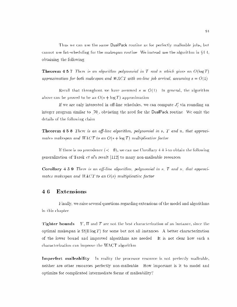
84
Thus we can use the same DualPack routine as for perfectly malleable jobs, but
cannot use list-scheduling for the makespan routine. We instead use the algorithm in x4.4,obtaining the following.
Theorem 4.5.7 There is an algorithm polynomial in T and n which gives an O(logT )
approximation for both makespan and WACT with on-line job arrival, assuming s = O(1).
Recall that throughout we have assumed s = O(1). In general, the algorithm
above can be proved to be an O(s+ logT ) approximation.
If we are only interested in o�-line schedules, we can compute J 0`via rounding an
integer program similar to [70], obviating the need for the DualPack routine. We omit the
details of the following claim.
Theorem 4.5.8 There is an o�-line algorithm, polynomial in s, T and n, that approxi-
mates makespan and WACT to an O(s+ log T ) multiplicative factor.
If there is no precedence (�= ;), we can use Corollary 4.4.5 to obtain the followinggeneralization of Turek et al's result [112] to many non-malleable resources.
Corollary 4.5.9 There is an o�-line algorithm, polynomial in s, T and n, that approxi-
mates makespan and WACT to an O(s) multiplicative factor.
4.6 Extensions
Finally, we raise several questions regarding extensions of the model and algorithms
in this chapter.
Tighter bounds. V , � and T are not the best characterization of an instance, since the
optimal makespan is (� logT ) for some but not all instances. A better characterization
of the lower bound and improved algorithms are needed. It is not clear how such a
characterization can improve the WACT algorithm.
Imperfect malleability. In reality the processor resource is not perfectly malleable,
neither are other resources perfectly non-malleable. How important is it to model and
optimize for complicated intermediate forms of malleability?
85
Persistent resources. A job may allocate memory mid-way through execution. We
cannot model this by a chain of two jobs, since the memory the job was already holding is
not released. How can jobs with such persistent resource needs be scheduled?
Non-clairvoyance and preemption. For the motivating applications, reasonable es-
timates of job running time are possible. More general purpose schedulers must be
non-clairvoyant, i.e., work without knowledge of tj before j completes [105, 92]. To handle
this, recourse to job preemption or cancellation is needed, whose large cost has to be factored
into the algorithm.
Arbitrary DAGs. While we have handled hierarchical job graphs such as forests or series-
parallel graphs, the general DAG case is open. It is known that precedence-constrained
knapsack with general precedence is strongly NP-hard [75], unlike forests. We show that
settling the approximability issue will be challenging [4]. This shows that the framework of
[70] may need modi�cation to handle DAG's, not necessarily that the scheduling problem
is di�cult.
Claim 4.6.1 There is an approximation preserving reduction from Expansion, the problem
of estimating the vertex expansion of a bipartite graph, to P.O.K., the partial order knapsack
problem, even when all item costs and pro�ts are restricted to f0; 1g.
Proof. Given G = (L;R;E), suppose we need the vertex expansion of R. Construct a two
layer partial order �: the upper layer contains a job j for every u 2 L, with c(j) = 1,
p(j) = 0. The lower layer contains a job j for every v 2 R, with c(j) = 0, p(j) = 1. E is
directed from L to R. Run the routine for P.O.K. n times, with target pro�ts P 2 f1; : : : ; ng.Return minP fC(P )=Pg, where C(P ) is the cost returned for target pro�t P .
Flowtime. In this chapter we consider maxj Cj and
PjwjCj ; some more ambitious
objective functions are
Pj(Cj � aj) and
Pj wj(Cj � aj), commonly called owtime.
Unfortunately, even with a single machine, o�-line problem instance, and no resource or
precedence constraints, it is NP-hard to approximate non-preemptive owtime better thanabout a factor of (
pn) [80]. In a practical implementation of our algorithm, one might
arti�cially increase wj for jobs waiting for a long time.
86
Chapter 5
Dynamic scheduling using parallel
random allocation
5.1 Introduction
Thus far in the thesis we have developed scheduling algorithms for problems with
one benign feature: when a job arrives at the scheduler, its resource requirements and
running time can be estimated. For the scienti�c problem domain addressed so far, this is
a reasonable assumption. However, in more dynamic and irregular programs, the scheduler
may not have any knowledge of the running time of jobs or tasks prior to completion.
Schedulers that produce schedules without this knowledge are called non-clairvoyant. There
are a few techniques to handle non-clairvoyant scenarios, depending on the cost model and
the optimization objective.
In the simplest non-clairvoyant model, the goal is to minimize the �nish time of
a dynamically growing task graph, and there is a central pool in which all ready jobs are
placed. Assuming that shared access to the central pool takes zero time, Graham analyzed
the makespan of the resulting schedule (called a list-schedule) and showed that it is less
than a factor of two worse than the optimal makespan [64].
This solution has a communication bottleneck problem: all processors access the
central pool. The overhead can be especially large for �ne-grain tasks. One technique to
reduce the overhead is to let each processor have a local task pool from which it removes
and executes some task, if any. New tasks are sent to the pool of a processor chosen
87
uniformly at random. Karp and Zhang analyzed the performance of this strategy for
unit-time tasks. In x5.2 we extend the analysis to handle arbitrary unknown task times
without preemption, i.e., tasks run to completion once they are started. (If arbitrarily
frequent preemption is permitted, the unknown time case is no di�erent from the unit-time
case. We mention in passing that for the weighted average completion time metric, the only
known non-clairvoyant approximation algorithms use preemption every time-step.)
The chapter continues in x5.3 with the study of an extension of random allocation
in a distributed setting. In the previous model, each task was assigned a random destination
only once, independent of where other tasks were sent. Roughly speaking, a single round
of random allocation gives a logarithmic smoothing of load. As a more precise example,
when n balls are thrown independently and uniformly at random into n bins, the number of
balls in the most heavily loaded bin is �(logn= log logn), with probability over 1�O(1=n).
Note that balls do not need to communicate with each other, and only one round of random
throwing is needed. We show how the load imbalance can be decreased as we invest more
rounds of random throws (which implicitly propagates the load information).
Apart from the usual applications in distributed job scheduling, such multi-round
load distribution protocols may �nd other uses. For example, in a serverless distributed �le
system, newly created data blocks have to be assigned storage on the disk at one of the
workstations using the �le system. To distribute blocks evenly among the disks, we may
send each block to a random disk, or maintain global information about the number of free
blocks on each disk. Our analysis explores the trade-o� between these two extremes.
5.2 Random allocation for dynamic task graphs
We analyze the performance of random allocation schemes applied to irregular and
dynamic task-parallel programs. Execution of the program de�nes a job precedence graph
with vertices representing jobs and directed edges representing precedence constraints. The
precedence graph is revealed on-line and is irregular in shape, and the processing times of
jobs are diverse and unknown before job completion. The objective function to minimize
is makespan, the maximum completion time of a job. Although the exact problem is
NP-hard, good approximations are possible if the algorithm assigning jobs to processors is
centralized, and thus has perfect global knowledge. For example, Graham's list-scheduling
algorithm [64] will result in a �nish time at most 2 � 1=P times optimal, where P is the
88
number of processors. However, this may lead to a severe communication bottleneck at
the processor where the pool of jobs resides, especially for �ne-grained tasks. Our goal,
therefore, is to study decentralized allocation which avoids such bottlenecks.
The bottleneck can be relieved in a variety of ways, each of which reduces
communication cost by sacri�cing global load information and thus risking some load
imbalance. We study work sharing, where busy processors forward jobs to random
processors. Some other techniques are work stealing, where idle processors ask for work [19],
and di�usion, where neighbors exchange local load information and then move some jobs
from busy to lazy processors [61].
5.2.1 Models and notation
The input comprises a set J of jobs presented to the algorithm in a distributed and
on-line fashion. Job j has running time tj , also referred to as its \weight" (not to be confused
with \priority" as in Chapter 4). We assume these are powers of 2; this will a�ect the results
only in constant factors. We assume that tj can be known only when job j completes. The
total work or weight in a job set J is denoted t(J) =P
j2J tj . The number of jobs in J
is denoted n(J). The average job weight is t(J) = t(J)=n(J). Let tmax(J) = maxj2Jftjgand tmin(J) = minj2Jftjg, and let T (J) = tmax(J)=tmin(J). Equivalently we scale jobs
so that tmin = 1 and tmax = T . This is in keeping with recent analyses of on-line load
balancing algorithms [10], and is more broadly applicable than results with assumptions
about distribution or variance.
J will have an associated acyclic precedence relation � � J � J . Let �j =
maxj0�jf�j0g+ tj be the earliest time at which j can �nish given in�nitely many processors
(the de�nition is not circular since the precedence graph is acyclic). Let �(J) = maxj2Jf�jgbe the longest critical path. We assume there is a unique root job. The number of edges
on a path from j to the root is denoted h(j); the path will be clear from context. Also let
h(J) be the maximum number of edges on any precedence path in J .
J will be omitted when clear from context. We assume that job times and the job
graph are oblivious of the decisions made by the scheduler. In exhaustive traversal, J is
�nite and the goal is to execute all jobs in J in any order obeying �. In heuristic search
or branch and bound, the job graph J provided may be very large or even in�nite. Each
job j has an associated cost c(j), with the requirements that j1 � j2 ) c(j1) < c(j2) and
89
all costs are distinct without loss of generality. The goal of the execution is to start at the
root and execute jobs obeying �, until the leaf node with minimum cost c� is identi�ed. It
is not necessary to generate and execute all jobs in J .
Sequential algorithm. A common sequential strategy is the \best �rst" traversal. All
available jobs with completed predecessors are maintained in a priority queue. While the
queue is non-empty, the job j with least c(j) is removed and executed. The jobs executed
are ~J = fj 2 J : c(j) < c�g � J . In the special case of complete traversal, ~J = J . For all
models, we assume that operations on a priority queue for job selection take negligible time
compared to job execution time. In this model, the sequential algorithm takes time t( ~J).
We assume jJ j � j ~J j � P . The interesting case for us is when jJ j � j ~J j, so that work
stealing is not an option.
Parallel algorithm. Parallel execution starts with the root job in one processor. A job
can be started when all predecessors have been completed. When a processor completes
executing a job j, all successors of j become available to that processor. Processors can
negotiate to transfer available jobs among themselves.
There is no coordinated global communication for load balancing purposes. We
study the setting with a local priority queue of jobs in the memory of each processor as
in [78]. Thus, priority is preserved within each local queue but not across processors. An
idle processor non-preemptively executes the best job from its local queue, if any. Any
newly available job with completed predecessors is enqueued into the priority queue of a
processor chosen uniformly at random. The destination processor is not interrupted.
Communication. The machine model consists of processors with individual local
memory connected by a communication network. We ignore the topology of the interconnect
as in the LogP model [37]. Communicating a job takes unit time at the two processors
involved in the transfer.
Pruning and termination. In parallel branch and bound, each processor has to
periodically propagate the cost of the least cost leaf it has expanded, so that all processors
know the cost of the global best cost leaf in order to use it for pruning. Also, barrier
synchronizations are required to detect situations where all local queues are empty so
90
that the processors can terminate. We note that these can be done infrequently with
low overhead, so they do not a�ect the time bounds we derive.
5.2.2 Discussion of results
For exhaustive search ~J = J , and greedy centralized schedules give a simple bound
on makespan in terms of variables de�ned above: �(t=P+�), the average work per processor
plus the critical path length. We show that the situation changes somewhat in the branch
and bound setting: (t( ~J)P
+ h( ~J) � T (J)) may be necessary even for an ideal centralized
scheduler with no communication cost. Then we give an analysis of parallel branch and
bound with ~J 6= J in a complete network: we show that with probability at least 1 � �,
the makespan is O( tP+ hT log hT + T log
n
�), where t = t( ~J), h = h( ~J), n = n( ~J), and
T = T (J). We also report on experience with some irregular programs. This is necessary
for two reasons. First, our analysis is probabilistic and asymptotic; in practice, constant
factors would be important. Second, although the above result establishes near-optimal load
balance, our model does not re ect the gains from avoiding communication bottlenecks.
Other results of the di�usion type are based on occasionally matching busy and
idle processors and transferring jobs [61, 98]. These are not appropriate for relatively
�ne-grain jobs which is our focus. Notice also that diversity in job execution times makes
coordination even harder unless a processor can suspend long jobs and participate in global
communication.
Work stealing is the strategy of least communication for the particular case where
the job graph J is an out-tree, all jobs must be executed, and the relative order of execution
is immaterial (provided it obeys �). In work stealing, the graph is expanded depth-�rst
locally in each processor, and idle processors steal jobs nearest to the root [122, 19]. In
many application such as parallel search or branch and bound, the total work done is very
sensitive to the job order, and one wishes to deviate from the best sequential order as little
as possible [47, 8].
5.2.3 Weighted occupancy
At �rst we consider the weighted occupancy problem, where there is no precedence
among jobs. There are n weighted balls (jobs), ball j having weight tj . These balls are
thrown uniformly at random into P bins (processors). We want to bound the weight of the
91
heaviest bin.
Lemma 5.2.1 For random allocation of weighted balls to bins, with probability at least 1��,each bin has O( t
P+ T (log log T + log
P
�)) weight.
Proof. Classify the balls into weights 1; 2; : : : ; T , where there are ni balls of weight 2i. Fix
one bin. The probability that there are at least mi balls of weight 2iin this bin is at most�
ni
mi
�P�mi � (
eni
Pmi)mi , which is less that
�
P logT for mi = O(niP+ log logT + log
P
�). Adding
over i and all P bins gives the result.
5.2.4 Delay sequence
Next, we show an upper bound for random allocation. Unlike in the previous
section, occupancy results cannot be used directly, since unlike a batch, a DAG schedule
cannot be composed from arbitrary task subsets. Further, in analyses related to global
task pools as above, arguments depend signi�cantly on statements to the e�ect that during
certain intervals of time, most processors do useful work. We can no longer say this when
each processor has a local task pool: processors can remain idle even though there are tasks
yet to expand, because they can be in the queues of other processors. We handle this using
a delay sequence argument. The following lemma is similar to Ranade's construction [96].
Lemma 5.2.2 Suppose the execution �nishes at time � . Then the following 4-tuple
(s; Q;R;�) exists:
� s is a job that �nished no earlier than � . Let S = (s1; : : : ; sh(s)) be a path of \special"
jobs from the root of the DAG to job s = sh(s).
� Q = (q1; : : : ; qh(s)) is an ordered list, where q` is the processor that executed s`, for
1 � ` � h(s).
� R � ~J is a set of jobs, and
� �1; : : : ;�h(s) is a partition of [1; � ] such that
{ R \ fs1; : : : ; sh(s)g = ;.{ Each job in R become \ready" and arrives into qj during interval �j , for some
j, 1 � j � h(s).
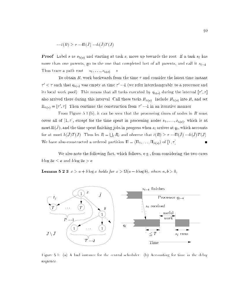
92
{ t(R) � � ��( ~J)� h( ~J)T (J).
Proof. Label s as sh(s) and starting at task s, move up towards the root. If a task s` has
more than one parents, go to the one that completed last of all parents, and call it s`�1.
Thus trace a path root = s1; : : : ; sh(s) = s.
To obtain R, work backwards from the time � and consider the latest time instant
� 0 < � such that qh(s) was empty at time �0�1 (we refer interchangeably to a processor and
its local work pool). This means that all tasks executed by qh(s) during the interval [� 0; � ]
also arrived there during this interval. Call these tasks Rh(s). Include Rh(s) into R, and set
�h(s) = [� 0; � ]. Then continue the construction from � 0 � 1 in an iterative manner.
From Figure 5.1 (b), it can be seen that the processing times of nodes in R must
cover all of [1; � ], except for the time spent in processing nodes s1; : : : ; sh(s), which is at
most �( ~J), and the time spent �nishing jobs in progress when s` arrives at q`, which accounts
for at most h( ~J)T (J). Thus let R =
S`R` and observe that t(R) � � ��( ~J)� h( ~J)T (J).
We have also constructed a ordered partition � = (�1; : : : ;�h(s)) of [1; � ].
We also note the following fact, which follows, e.g., from considering the two cases
b log 2a � a and b log 2a > a.
Lemma 5.2.3 x > a+ b logx holds for x > (a+ b log b), where a; b > 0,
� � �
� � �
J n ~J
1
1
1 1
T T
P � 1
T � 2
x
tj
s`�1 �nishes
useful
work
s` runs� T
y
Processor q`�1
s` received
q`
Time
~J
Figure 5.1: (a) A bad instance for the central scheduler. (b) Accounting for time in the delay
sequence.
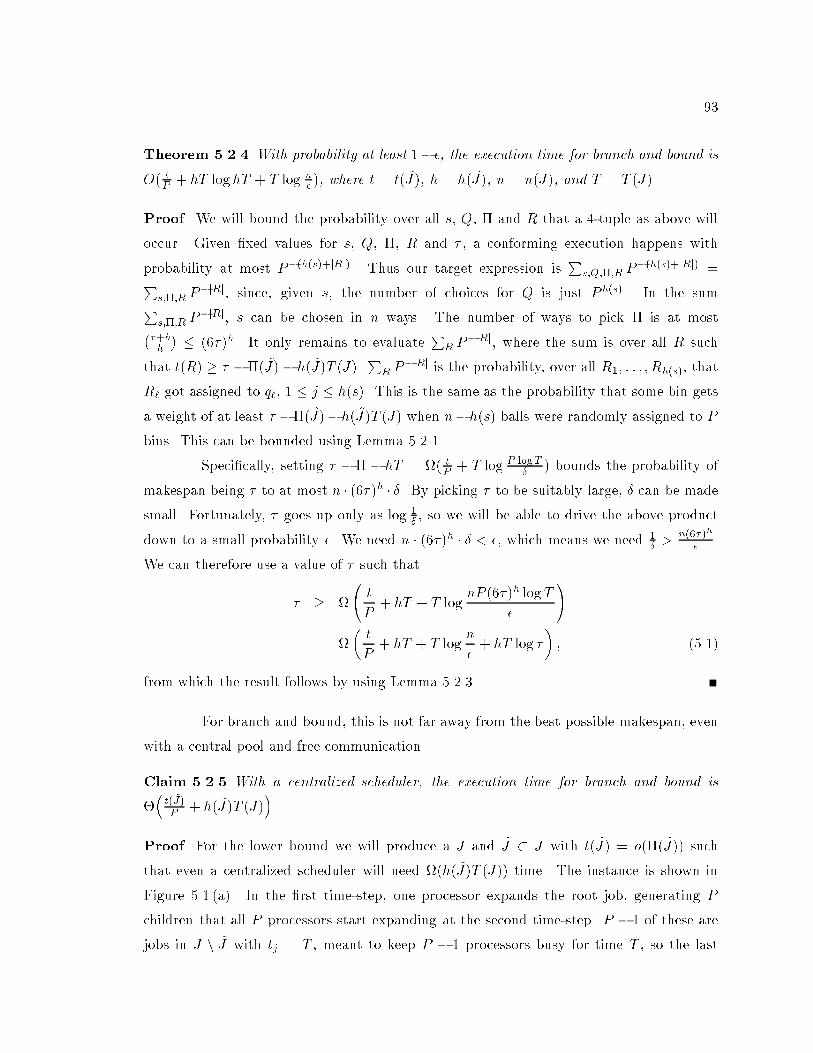
93
Theorem 5.2.4 With probability at least 1� �, the execution time for branch and bound is
O( tP+ hT log hT + T log
n
�), where t = t( ~J), h = h( ~J), n = n(J), and T = T (J).
Proof. We will bound the probability over all s, Q, � and R that a 4-tuple as above will
occur. Given �xed values for s, Q, �, R and � , a conforming execution happens with
probability at most P�(h(s)+jRj). Thus our target expression is
Ps;Q;�;R P
�(h(s)+jRj)=P
s;�;R P�jRj
, since, given s, the number of choices for Q is just Ph(s). In the sumP
s;�;R P�jRj
, s can be chosen in n ways. The number of ways to pick � is at most��+hh
� � (6�)h. It only remains to evaluate
PR P
�jRj, where the sum is over all R such
that t(R) � � ��( ~J)� h( ~J)T (J).P
RP�jRj is the probability, over all R1; : : : ; Rh(s), that
R` got assigned to q`, 1 � j � h(s). This is the same as the probability that some bin gets
a weight of at least � ��( ~J)� h( ~J)T (J) when n� h(s) balls were randomly assigned to P
bins. This can be bounded using Lemma 5.2.1.
Speci�cally, setting � � � � hT = (t
P+ T log
P logT�
) bounds the probability of
makespan being � to at most n � (6�)h � �. By picking � to be suitably large, � can be made
small. Fortunately, � goes up only as log1�, so we will be able to drive the above product
down to a small probability �. We need n � (6�)h � � < �, which means we need1�>
n(6�)h
�.
We can therefore use a value of � such that
� �
t
P+ hT + T log
nP (6�)h logT
�
!
=
�t
P+ hT + T log
n
�+ hT log �
�; (5.1)
from which the result follows by using Lemma 5.2.3.
For branch and bound, this is not far away from the best possible makespan, even
with a central pool and free communication.
Claim 5.2.5 With a centralized scheduler, the execution time for branch and bound is
�
�t( ~J)P
+ h( ~J)T (J)�.
Proof. For the lower bound we will produce a J and ~J � J with t( ~J) = o(�( ~J)) such
that even a centralized scheduler will need (h( ~J)T (J)) time. The instance is shown in
Figure 5.1 (a). In the �rst time-step, one processor expands the root job, generating P
children that all P processors start expanding at the second time-step. P � 1 of these are
jobs in J n ~J with tj = T , meant to keep P � 1 processors busy for time T , so the last
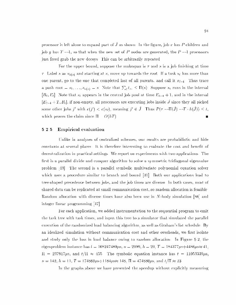
94
processor is left alone to expand part of ~J as shown. In the �gure, job x has P children and
job y has T � 1, so that when the new set of P nodes are generated, the P � 1 processors
just freed grab the new decoys. This can be arbitrarily repeated.
For the upper bound, suppose the makespan is � and s is a job �nishing at time
� . Label s as sh(s) and starting at s, move up towards the root. If a task s` has more than
one parent, go to the one that completed last of all parents, and call it s`�1. Thus trace
a path root = s1; : : : ; sh(s) = s. Note thatP
`ts` � �(s). Suppose s` runs in the interval
[B`; E`]. Note that s` appears in the central job pool at time E`�1 + 1, and in the interval
[E`�1+ T;B`], if non-empty, all processors are executing jobs inside~J since they all picked
some other jobs j0 with c(j0) < c(s`), meaning j0 2 ~J . Thus P (� � �( ~J) � T � h( ~J)) � t,
which proves the claim since � = O(hT ).
5.2.5 Empirical evaluation
Unlike in analyses of centralized schemes, our results are probabilistic and hide
constants at several places. It is therefore interesting to evaluate the cost and bene�t of
decentralization in practical settings. We report on experiments with two applications. The
�rst is a parallel divide and conquer algorithm to solve a symmetric tridiagonal eigenvalue
problem [43]. The second is a parallel symbolic multivariate polynomial equation solver
which uses a procedure similar to branch and bound [31]. Both our applications lead to
tree-shaped precedence between jobs, and the job times are diverse. In both cases, most of
shared data can be replicated at small communication cost, so random allocation is feasible.
Random allocation with diverse times have also been use in N -body simulation [86] and
integer linear programming [47].
For each application, we added instrumentation to the sequential program to emit
the task tree with task times, and input this tree to a simulator that simulated the parallel
execution of the randomized load balancing algorithm, as well as Graham's list schedule. By
an idealized simulation without communication cost and other overheads, we �rst isolate
and study only the loss in load balance owing to random allocation. In Figure 5.2, the
eigenproblem instance has t = 108247480�s, n = 2999, h = 20, T = 184377�s�4486�s� 41,
� = 237917�s, and t=� � 455. The symbolic equation instance has t = 11053339�s,
n = 142, h = 11, T = 174860�s�1184�s� 148, � = 474880�s, and t=� � 23.
In the graphs above we have presented the speedup without explicitly measuring
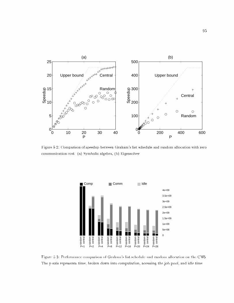
95
0 10 20 30 400
5
10
15
20
25
P
Spe
edup
(a)
Upper bound Central
Random
0 200 400 6000
100
200
300
400
500
P
Spe
edup
(b)
Upper bound
Central
Random
Figure 5.2: Comparison of speedup between Graham's list schedule and random allocation with zero
communication cost. (a) Symbolic algebra, (b) Eigensolver.
Comp Comm Idle
0
5e+08
1e+09
1.5e+09
2e+09
2.5e+09
3e+09
3.5e+09
4e+09
ran
dom
cen
tral
P=1
ran
dom
cen
tral
P=2
ran
dom
cen
tral
P=4
ran
dom
cen
tral
P=8
ran
dom
cen
tral
P=12
ran
dom
cen
tral
P=16
ran
dom
cen
tral
P=20
ran
dom
cen
tral
P=24
ran
dom
cen
tral
P=28
Figure 5.3: Performance comparison of Graham's list schedule and random allocation on the CM5.
The y-axis represents time, broken down into computation, accessing the job pool, and idle time.
96
communication costs. We also measured actual speedup on the CM5 multiprocessor.
Comparing the speedup curves enabled us to judge the closeness of the simulation to
reality. In Figure 5.3, we present a break-up analysis of parallel running time for the
eigensolver, comparing a centralized task queue with the random distributed allocation.
Although load imbalance is larger for random allocation, the bene�t due do decentralization
is overwhelming.
5.2.6 Discussions
Several questions arise from this and related results. It would be interesting to
tighten the makespan estimates in this section, as well as to provide randomized lower
bounds. The performance of multiple round strategies [9, 1] for dynamic job graphs remains
open, as is their e�ect on further reducing the load imbalance. Finally, extending the results
to capture network contention as in the atomic message model [86] seems like a natural goal.
5.3 Multi-round load balancing protocols
The goal of this section is to generalize single round random allocations to multiple
rounds, aided by spreading load information, to facilitate better load balance. It is well
known that when n balls are thrown independently and uniformly at random into n bins,
with high probability (by which we shall mean 1 � O( 1n)) the maximum number of balls
received by any bin is �(logn
log logn) [93]. Recently, an important extension of this result was
proven by Azar et al [9]. Suppose we place the balls sequentially, one at a time; for each ball,
we choose two bins independently and uniformly at random, and place the ball in the less
full bin. When all the balls have been placed, the fullest bin contains only �(log log n) balls
with high probability, an exponential improvement over the simple randomized approach.
Notice that in both these cases, the expected number of balls in a bin is one, but the
maximum occupancy grows with n, with the obvious implication that any technique for
reducing the gap between the expected and maximum occupancy may be useful for load
balancing parallel jobs. For example, such logarithmic terms appeared in the analysis in
x5.2.We mention a few scenarios that motivate a detailed study of the trade-o�
between the investment in communication rounds and the resulting load balance. The
�rst motivation is directly from the analysis in x5.2, where the randomized upper bounds
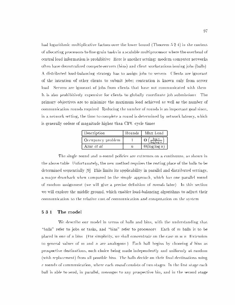
97
had logarithmic multiplicative factors over the lower bound (Theorem 5.2.4) in the context
of allocating processors to �ne-grain tasks in a scalable multiprocessor where the overhead of
central load information is prohibitive. Here is another setting: modern computer networks
often have decentralized compute-servers (bins) and client workstations issuing jobs (balls).
A distributed load-balancing strategy has to assign jobs to servers. Clients are ignorant
of the intention of other clients to submit jobs; contention is known only from server
load. Servers are ignorant of jobs from clients that have not communicated with them.
It is also prohibitively expensive for clients to globally coordinate job submissions. The
primary objectives are to minimize the maximum load achieved as well as the number of
communication rounds required. Reducing the number of rounds is an important goal since,
in a network setting, the time to complete a round is determined by network latency, which
is generally orders of magnitude higher than CPU cycle times.
Description Rounds Max Load
Occupancy problem 1 �
�logn
log logn
�Azar et al n �(log log n)
The single round and n-round policies are extremes on a continuum, as shown in
the above table. Unfortunately, the new method requires the resting place of the balls to be
determined sequentially [9]. This limits its applicability in parallel and distributed settings,
a major drawback when compared to the simple approach, which has one parallel round
of random assignment (we will give a precise de�nition of rounds later). In this section
we will explore the middle ground, which enables load-balancing algorithms to adjust their
communication to the relative cost of communication and computation on the system.
5.3.1 The model
We describe our model in terms of balls and bins, with the understanding that
\balls" refer to jobs or tasks, and \bins" refer to processors. Each of m balls is to be
placed in one of n bins. (For simplicity, we shall concentrate on the case m = n. Extension
to general values of m and n are analogous.) Each ball begins by choosing d bins as
prospective destinations, each choice being made independently and uniformly at random
(with replacement) from all possible bins. The balls decide on their �nal destinations using
r rounds of communication, where each round consists of two stages. In the �rst stage each
ball is able to send, in parallel, messages to any prospective bin, and in the second stage
98
each bin is able to send, in parallel, messages to any ball from which it has ever received a
message. In the �nal round, the balls commit to one of the prospective bins and the process
terminates. Messages are assumed to be of size polylog(n;m). The goal is to minimize
the maximum load, which is de�ned to be the maximum number of balls in any bin upon
completion.
5.3.2 Summary of results
Our main goal is to develop and analyze a multiple round protocol for assigning
balls to bins. Informally, for each round, each bin sets a threshold T , and accepts up to
T balls in that round. Excess balls are thrown to a random destination again. Clearly,
increasing T will complete the protocol in a few communication steps, but the maximum
bin load will be large. On the other hand, reducing T limits the maximum load at the
expense of many rounds. We will quantify this trade-o� in x5.3.3.Our analysis exploits a basic tool that expresses the relation between occupancy
distributions and Poisson distributions [63, 1]. Using this tool, we show that after a �xed
number of rounds r, the �nal maximum load is O�
r
qlogn
log logn
�with high probability.
We also show via lower bounds that no better load balance can be achieved by
a large class of load balancing algorithms. The class that we restrict our attention to are
non-adaptive, in that the possible destinations are chosen before any communication takes
place. We will also restrict our discussion to strategies that are symmetric, in the sense
that all balls and bins perform the same underlying algorithm and all possible destinations
are chosen independently and uniformly at random. We believe that these restrictions have
practical merit, as an algorithm with these properties would be easier to implement. We
provide a lower bound for non-adaptive and symmetric strategies. For any �xed number r
of rounds of communication and any �xed number d of choices for each ball, we show that
with constant probability the maximum load is at least
�r
qlogn
log logn
�.
5.3.3 Threshold protocol
Balls and bins execute the following protocol, which we call Threshold(T ).
1. While there exists a ball that has not been assigned to a bin do the following round
of steps.
2. In parallel, each unaccepted ball chooses a random bin and sends it a request.
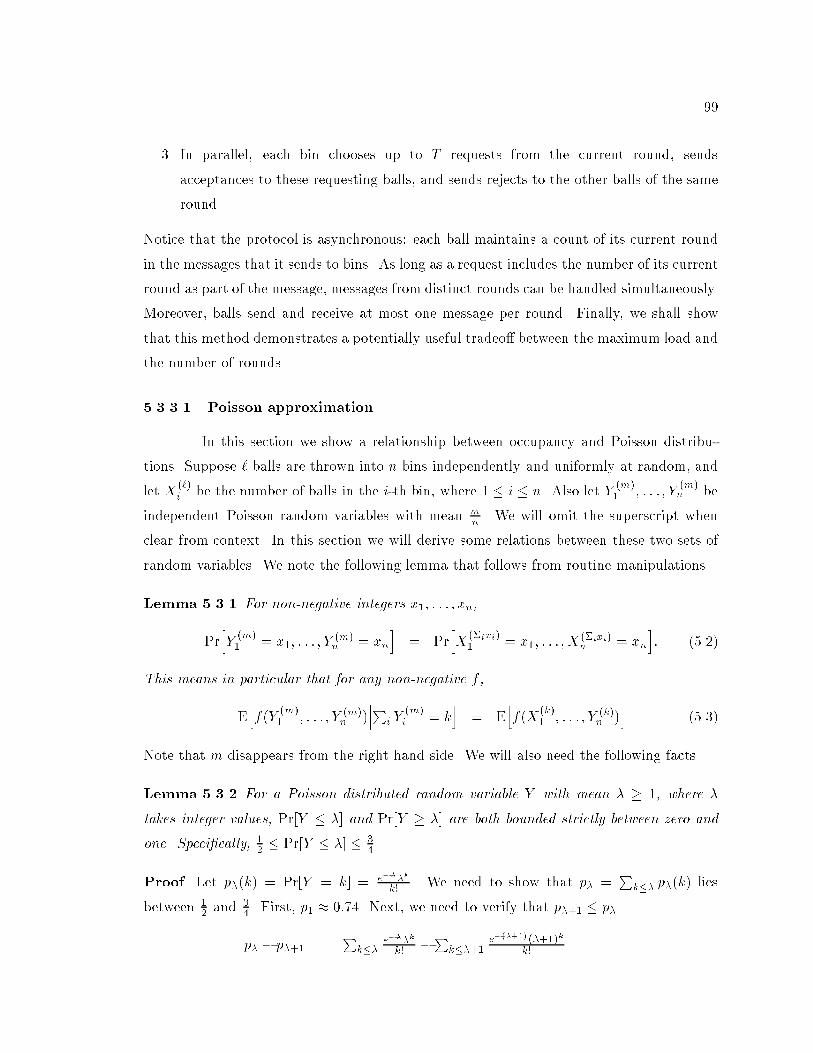
99
3. In parallel, each bin chooses up to T requests from the current round, sends
acceptances to these requesting balls, and sends rejects to the other balls of the same
round.
Notice that the protocol is asynchronous: each ball maintains a count of its current round
in the messages that it sends to bins. As long as a request includes the number of its current
round as part of the message, messages from distinct rounds can be handled simultaneously.
Moreover, balls send and receive at most one message per round. Finally, we shall show
that this method demonstrates a potentially useful tradeo� between the maximum load and
the number of rounds.
5.3.3.1 Poisson approximation
In this section we show a relationship between occupancy and Poisson distribu-
tions. Suppose ` balls are thrown into n bins independently and uniformly at random, and
let X(`)i
be the number of balls in the i-th bin, where 1 � i � n. Also let Y(m)1 ; : : : ; Y
(m)n be
independent Poisson random variables with meanm
n. We will omit the superscript when
clear from context. In this section we will derive some relations between these two sets of
random variables. We note the following lemma that follows from routine manipulations.
Lemma 5.3.1 For non-negative integers x1; : : : ; xn,
Pr
hY(m)1 = x1; : : : ; Y
(m)n = xn
i= Pr
hX
(�ixi)1 = x1; : : : ; X
(�ixi)n = xn
i: (5.2)
This means in particular that for any non-negative f ,
E
hf(Y
(m)1 ; : : : ; Y (m)
n )
���Pi Y(m)i
= ki
= E
hf(X
(k)1 ; : : : ; Y (k)
n )
i(5.3)
Note that m disappears from the right hand side. We will also need the following facts.
Lemma 5.3.2 For a Poisson distributed random variable Y with mean � � 1, where �
takes integer values, Pr[Y � �] and Pr[Y � �] are both bounded strictly between zero and
one. Speci�cally, 12 � Pr[Y � �] � 3
4 .
Proof. Let p�(k) = Pr[Y = k] = e��
�k
k! . We need to show that p� =
Pk�� p�(k) lies
between12 and
34 . First, p1 � 0:74. Next, we need to verify that p�+1 � p�.
p� � p�+1 =
Pk��
e��
�k
k! �Pk��+1e�(�+1)(�+1)k
k!
100
= e�(�+1)hP
k��e�
k�(�+1)kk! � (�+1)�
�!
i� e
�(�+1)
�!
hPk��
�e�k � (�+ 1)
k
�� (�+ 1)
�
i� e
�(�+1)
�(��1)�!he��+2 � �(�+ 1)
� � (e� 1)�� 1
i:
The expression in brackets is at least
���e�2 � �(1 + 1
�)�
�� (e� 1)�� 1 � e��+1(�� 1)� (e� 1)�� 1;
which is positive for all � � 2.
Finally, we apply the Central Limit Theorem [53] to observe that lim�!1 p� =12.
Let fXig be a sequence of n iid random variables. Suppose the expectation
� = E[Xi] and variance �2 = V[Xi] exist and let Sn =
PiXi. Then for every
�xed �,
limn!1Pr
�Sn � n�
�pn
< �
�= �(�);
where �(x) = Pr[X � x], and X is a normally distributed random variable with
E[X ] = 0 and V[X ] = 1.
As an immediate corollary, let there be n = � Poisson distributed variables each
with � = � = 1. Then Sn is distributed Poisson with mean and variance �, i.e., Sn � Y .
Now letting � = 0 gives the result.
Theorem 5.3.3 If f(x1; : : : ; xn) be a non-negative function, then
E
hf(X
(m)1 ; : : : ; X(m)
n )
i�
p2�mE
hf(Y
(m)1 ; : : : ; Y (m)
n )
i: (5.4)
Further if Ehf(X
(k)1 ; : : : ; X
(k)n )
iis monotonically increasing with k, then
E[f(X1; : : : ; Xn)] � 4 � E[f(Y1; : : : ; Yn)]: (5.5)
Similarly if Ehf(X
(k)1 ; : : : ; X
(k)n )
iis monotonically decreasing with k, then
E[f(X1; : : : ; Xn)] � 2 � E[f(Y1; : : : ; Yn)]: (5.6)
Proof. We have that
E
hf(Y
(m)1 ; : : : ; Y (m)
n )
i=
Xk�0
E
hf(Y
(m)1 ; : : : ; Y (m)
n )
���Pi Y(m)i
= ki� Pr
hPi Y
(m)i
= ki
=
Xk�0
E
hf(X
(k)1 ; : : : ; X(k)
n )
i� Pr
hPi Yi = k
i; using (5.3)
� E
hf(X
(m)1 ; : : : ; X(m)
n )
i� Pr
hPi Yi = m
i:
101
Equation (5.4) now follows by noting that Pr[�iYi = m] =mme�m
m!and applying Stirling's
approximation.
If E
hf(X
(k)1 ; : : : ; X
(k)n )
iincreases with k, then by a similar argument we have
E
hf(Y
(m)1 ; : : : ; Y (m)
n)] =
Xk�0
E
hf(X
(k)1 ; : : : ; X(k)
n)
i�Pr
hPiYi = k
i; using (5.3)
� E
hf(X
(m)1 ; : : : ; X(m)
n)
i�Pr
hPiYi � m
iSince E[�iYi] = m, Lemma 5.3.2 says that Pr[�iYi � m] � 1
4, and (5.5) follows. The
derivation of (5.6) is similar.
In what follows, we will use \[c]" to stand for the indicator Ic which has value one if condition
c is true, zero otherwise.
Example 5.3.4 Suppose we want to show that the number of bins with at least � balls is
not likely to be much larger than B, for appropriate � and B. De�ne f as follows:
f(x1; : : : ; xn) =
hPi[xi � �] > B
i:
Since Ehf(X
(k)1 ; : : : ; X
(k)n )
iincreases with k, we can upper bound the probability that more
than B bins have at least � balls each, by the probability that I = �iIi > B, where
Ii =hY(m)i
� �i, where the Yi's are iid Poisson with mean
m
n. For m � n, � > 2 will su�ce
to infer that Pr[Yi � �] � 2Pr[Yi = �] � 2�! . Note also that Pr[Yi � �] � Pr[Yi = �]. 2
5.3.3.2 Upper bound for Threshold
Theorem 5.3.5 For m = n balls, if r is �xed independent of n, then Threshold(T )
terminates after r rounds with high probability, where T = O�
r
qr lognlog logn
�.
Proof. Let kj be the number of balls to be (re)thrown after j rounds (k0 = n). We will
show by induction that
kj � n
�4 logn
T !
�Tj�1T�1
(5.7)
with high probability (by which we mean 1 � O( 1na) for a suitably large constant a). The
case j = 0 is readily veri�ed. Now consider the situation when kj balls are thrown into n
bins in the (j + 1)-st round. For large enough n, kj=n � 1 < T for all j 2 f0; : : : ; rg.
102
Moving freely between the occupancy and the Poisson case by virtue of Theo-
rem 5.3.3, we can now proceed as in Example 5.3.4 to obtain that
e�kj=n(kj=n)T
T !� Pr[Ii = 1] � 2e�kj=n(kj=n)T
T !: (5.8)
the expected number Ii's that are ones is at most2ne
�kj=n(kj=n)T
T !. Now we use the simple
version of Cherno� bound, which says that for n Bernoulli trials with success probability p,
and 0 < � � 1, the number of successes Sn obeys Pr[Sn � (1+ �)np] � e��2np=3
. In our case
p = Pr[Ii = 1]. By setting � = 1 and verifying that np � a logn for a suitably large constant
a (this su�ces since r is constant too), we get that with high probability, after the (j+1)-st
round, w.h.p. the number of bins with more than T balls is at most4ne�kj=n(kj=n)
T
T ! . We can
make the conservative upper bound assumption that with probability exponentially close
to one, none of these over-full bins have more than logn balls in it, so that w.h.p.,
kj+1 � 4ne�kj=n lognT !
�4 logn
T !
�T (Tj�1)
T�1
� n
�4 logn
T !
�1+T (Tj�1)
T�1
= n
�4 logn
T !
�T (Tj+1�1)
T�1
: (5.9)
The induction follows. It only remains to verify that for constants r and 0 < � < 1, and
suitably large n, T = O�
r
qr lognlog logn
�su�ces to reduce kr�1 to less than n1��, at which point
one more round su�ces. This immediately implies a maximum load of O(rT ), which, for
�xed r, is O( rplogn= log logn).
Some additional bounds can be derived for non-constant r. In particular, for T = 1, one
can show that r = �(log logn) w.h.p.
5.3.3.3 Lower bound
In this section we will show a matching lower bound for �xed r. We can show
directly that the Threshold protocol will need (r) rounds to complete given a choice of T
only slightly smaller than the above choice in the upper bound case. More generally, we
can show this property for all symmetric, non-adaptive protocols.
Symmetric, non-adaptive protocols can be modeled using an edge orientation
setting. Consider the case of n balls and n bins. Each ball is an vertex in an n-vertex
graph. Initially, n random undirected edges are added to the graph, where by \random" we
103
mean that for each edge, independent of others, the two endpoints are chosen uniformly at
random (the issue of self-loops does not a�ect the asymptotic analysis). Choosing a �nal
destination is equivalent to choosing an orientation for the edge. The goal of the algorithm
is to minimize the maximum indegree over all vertices of the graph. In the case where there
are n balls and n bins, the corresponding graph is a random graph from Gn;n, the set of allgraphs with n vertices and n edges.
De�nition 5.3.6 Let N(x) be the edges incident with vertex x. The (r; x)-neighborhood
of an edge e = (x; y), denoted by Nr;x(e), is de�ned inductively by: N1;x(e) = N(x)� feg,Nr;x(e) = N(Nr�1;x(e))� feg.
A ball (edge) (x; y) gets confused about which way to orient if large neighborhoods
of both the endpoints are isomorphic. Speci�cally, suppose we invest r rounds of
communication. In each round of communication, a ball discovers a little more about
the graph. Speci�cally, since we want lower bounds, we may assume that the bins transport
all available information about the balls whenever possible. In r rounds, a ball e = (x; y)
knows everything about the balls in Nr;x(e)[Nr;y(e), and no more, before it must commit
to a bin; this follows from a simple induction argument. Suppose Nr;x(e) and Nr;y(e) are
isomorphic trees rooted at x and y. Then the ball has no reason to prefer one bin over
another, and must essentially choose randomly between bins x and y.
Obvious tie-breaking schemes do not a�ect the lower bound. For instance, if the
balls are ordered at the bins, either by random I.D. numbers or by a random permutation,
and then choose a bin according to their rank, the balls are essentially choosing a bin at
random. The proof can easily be modi�ed also for the case where the balls are ranked at
the bins by some �xed ordering, by using the symmetry of the destination choices of the
balls.
If many confused balls are incident on one bin, with constant probability, over half
of them will opt for the bin, which will become overloaded. We thus need to show that for
r and T suitably related to n, a random graph G 2 Gn;n has, with high probability, a near
isolated (T; r)-tree, de�ned as follows (see Figure 5.4).
1. It is a rooted balanced tree of depth r. All the leaves are at depth r.
2. The root has out-degree T . Internal nodes have one parent and T � 1 children.

104
Overloaded bin
level r � 1
level r
(T � 1)r
T � 1
(T � 1)r�1
level 0
level 1
T children
T � 1
v
z
Confused ball
Figure 5.4: A (T; r)-tree with confused balls.
3. The tree is near-isolated in the sense that no edge of G other than the tree edges are
incident to any internal node of the tree.
Theorem 5.3.7 With constant probability, a random graph from Gn;n contains a near-
isolated (T; r)-tree for �xed r and T = (rplogn= log logn). Assuming confused balls pick
each bin with probability 12, some bin will have load (T ) with constant probability.
Proof. A (T; r)-tree has
X(T;r) = 1 + TP
0�k<r (T � 1)k
= 1 + T(T�1)r�1
T�2 � T rvertices,
Y(T;r) = 1 + TP
0�k<r�1 (T � 1)k
= 1 + T(T�1)r�1�1
T�2 � T r�1
vertices incident only on internal edges, and Z(T;r) = X(T;r)�1 internal edges. We will drop
the subscript (T; r) from X , Y , and Z when clear from context.
Let ~v = (v1; : : : ; vX) be a sequence of X(T;r) vertices, and let I~v be the indicator
for \~v is a near-isolated (T; r)-tree," with v1 being the root, v2; : : : ; vT+1 being the �rst
level children, and so on. Let I =
P~v I~v . Note that I is not an indicator; it is a
non-negative integer random variable. For such variables it is routine to verify that
Pr[I = 0] � 1� E[I ]2=E[I2]. We will use this inequality to show that Pr[I = 0] is strictly
less than one; for this we will bound E[I ] from below and E[I2] from above by appropriate
constants in the next two lemmas.
Lemma 5.3.8 E[I ] is at least a constant for �xed r and T = (rplogn= log logn).
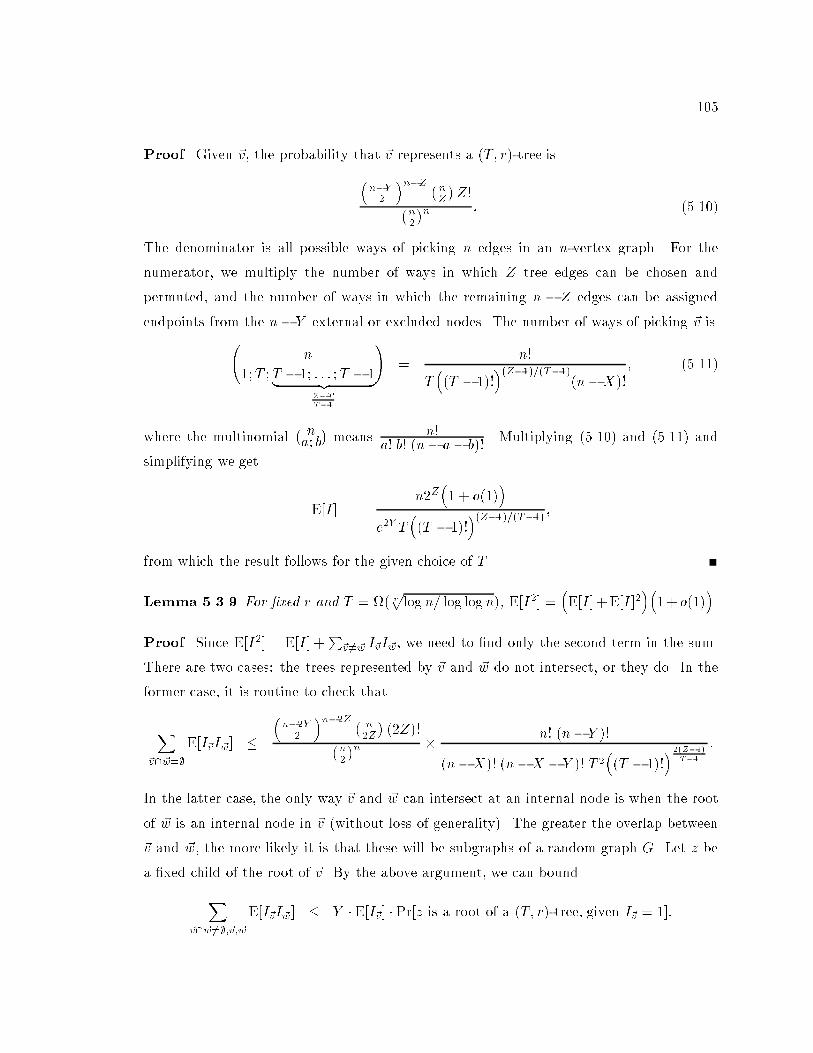
105
Proof. Given ~v, the probability that ~v represents a (T; r)-tree is
�n�Y2
�n�Z �
n
Z
�Z!�
n
2
�n : (5.10)
The denominator is all possible ways of picking n edges in an n-vertex graph. For the
numerator, we multiply the number of ways in which Z tree edges can be chosen and
permuted, and the number of ways in which the remaining n � Z edges can be assigned
endpoints from the n� Y external or excluded nodes. The number of ways of picking ~v is n
1;T ;T � 1; : : : ;T � 1| {z }Z�TT�1
!=
n!
T�(T � 1)!
�(Z�1)=(T�1)(n�X)!
; (5.11)
where the multinomial
� na; b�means
n!a! b! (n� a� b)!
. Multiplying (5.10) and (5.11) and
simplifying we get
E[I ] =
n2Z�1 + o(1)
�e2Y T
�(T � 1)!
�(Z�1)=(T�1) ;from which the result follows for the given choice of T .
Lemma 5.3.9 For �xed r and T = (rplog n= log logn), E[I2] =
�E[I ]+E[I ]2
��1+ o(1)
�.
Proof. Since E[I2] = E[I ] +P
~v 6=~w I~vI~w, we need to �nd only the second term in the sum.
There are two cases: the trees represented by ~v and ~w do not intersect, or they do. In the
former case, it is routine to check that
X~v\~w=;
E[I~vI~w] ��n�2Y2
�n�2Z �
n
2Z
�(2Z)!�
n
2
�n � n! (n� Y )!
(n�X)! (n�X � Y )! T 2�(T � 1)!
�2(Z�1)
T�1
:
In the latter case, the only way ~v and ~w can intersect at an internal node is when the root
of ~w is an internal node in ~v (without loss of generality). The greater the overlap between
~v and ~w, the more likely it is that these will be subgraphs of a random graph G. Let z be
a �xed child of the root of ~v. By the above argument, we can bound
X~v\~w6=;;~v; ~w
E[I~vI~w ] � Y � E[I~v] �Pr[z is a root of a (T; r)-tree, given I~v = 1]:
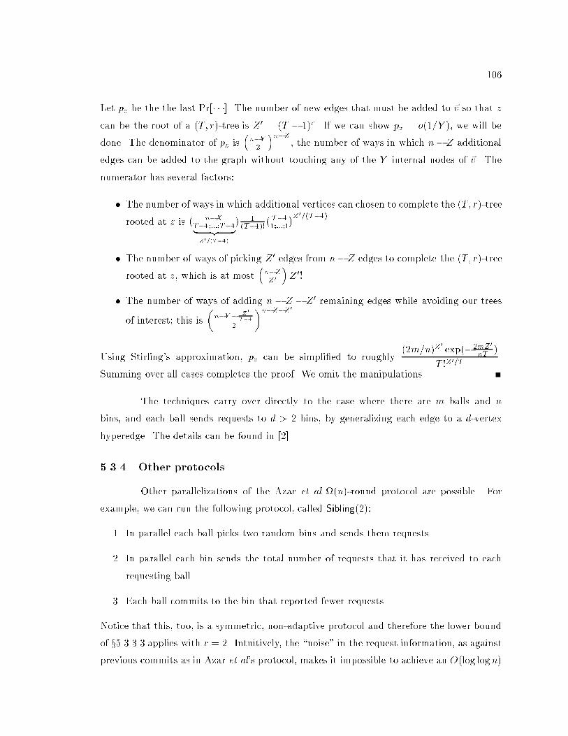
106
Let pz be the the last Pr[� � �]. The number of new edges that must be added to ~v so that z
can be the root of a (T; r)-tree is Z0 = (T � 1)r. If we can show pz = o(1=Y ), we will be
done. The denominator of pz is�n�Y2
�n�Z
, the number of ways in which n� Z additional
edges can be added to the graph without touching any of the Y internal nodes of ~v. The
numerator has several factors:
� The number of ways in which additional vertices can chosen to complete the (T; r)-tree
rooted at z is�
n�XT�1;:::;T�1| {z }Z0=(T�1)
�1
(T�1)!�T�11;:::;1
�Z0=(T�1).
� The number of ways of picking Z0 edges from n� Z edges to complete the (T; r)-tree
rooted at z, which is at most
�n�ZZ0
�Z0!.
� The number of ways of adding n � Z � Z0 remaining edges while avoiding our trees
of interest; this is
�n�Y � Z0
T�1
2
�n�Z�Z0.
Using Stirling's approximation, pz can be simpli�ed to roughly
(2m=n)Z0
exp(�2mZ0
nT)
T !Z0=T
.
Summing over all cases completes the proof. We omit the manipulations.
The techniques carry over directly to the case where there are m balls and n
bins, and each ball sends requests to d > 2 bins, by generalizing each edge to a d-vertex
hyperedge. The details can be found in [2].
5.3.4 Other protocols
Other parallelizations of the Azar et al (n)-round protocol are possible. For
example, we can run the following protocol, called Sibling(2):
1. In parallel each ball picks two random bins and sends them requests.
2. In parallel each bin sends the total number of requests that it has received to each
requesting ball.
3. Each ball commits to the bin that reported fewer requests.
Notice that this, too, is a symmetric, non-adaptive protocol and therefore the lower bound
of x5.3.3.3 applies with r = 2. Intuitively, the \noise" in the request information, as against
previous commits as in Azar et al's protocol, makes it impossible to achieve an O(log logn)
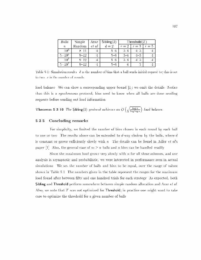
107
Balls Simple Azar Sibling(2) Threshold(T )
n Random et al d = 2 r = 2 r = 3 r = 5
106
8{11 4 5{6 5{6 4{5 4
5 � 106 9{12 4 5{6 5{6 4{5 4
107
9{12 4 5{6 5{6 4{5 4
5 � 107 9{12 4 5{6 6 5 4
Table 5.1: Simulation results. d is the number of bins that a ball sends initial request to; this is set
to two. r is the number of rounds.
load balance. We can show a corresponding upper bound [1]; we omit the details. Notice
that this is a synchronous protocol; bins need to know when all balls are done sending
requests before sending out load information.
Theorem 5.3.10 The Sibling(2) protocol achieves an O�q
lognlog logn
�load balance.
5.3.5 Concluding remarks
For simplicity, we limited the number of bins chosen in each round by each ball
to one or two. The results above can be extended to d-way choices by the balls, where d
is constant or grows su�ciently slowly with n. The details can be found in Adler et al's
paper [1]. Also, the general case of m � n balls and n bins can be handled readily.
Since the maximum load grows very slowly with n for all these schemes, and our
analysis is asymptotic and probabilistic, we were interested in performance seen in actual
simulations. We set the number of balls and bins to be equal, over the range of values
shown in Table 5.1. The numbers given in the table represent the ranges for the maximum
load found after between �fty and one hundred trials for each strategy. As expected, both
Sibling and Threshold perform somewhere between simple random allocation and Azar et al.
Also, we note that T was not optimized for Threshold; in practice one might want to take
care to optimize the threshold for a given number of balls.
108
Chapter 6
Survey of related work
Scheduling and resource allocation problems have been studied extensively in all
the forms discussed in this thesis. In this chapter we review some of the major results in the
various areas. Most of the exact problems are NP-hard, sometimes in the strong sense, andtherefore the thrust is on developing good approximation algorithms. Particular technical
references and their relation with this thesis are given in speci�c chapters.
6.1 Communication scheduling
The results in Chapter 2 follow (and generalize) a large number of preliminary
results in communication optimization, such as message vectorizing, coalescing, and
redundancy elimination [72, 123, 20, 5, 21, 68]. Message vectorization is the technique of
hoisting communication of array elements or sections out of loops to produce a single large
message. Typically this works locally on single loop-nests [123, 72, 67, 83, 68]. As compilers
were applied to more complex code, eliminating redundant communication beyond single
loop-nests and even across procedures became essential. This was typically done by tracing
the uses of an array (section) to a de�ning statement, placing all the communication entries
after that def, and canceling subsumed communication entries [69].
Communication can also be regarded as invoking a long-lasting asynchronous
operation on the network \functional unit." To minimize the latency penalty for �ne-grain
communication, it helps to detect writes to shared memory that can be reordered or
overlapped without violating the programmer's view of consistency of program variables. An
early result in this direction �nds cycles of con icting reads and writes and inserts minimal
109
synchronization to break all cycles [102]. This technique has recently been improved for
single program multiple data (SPMD) sources [82]. Another related area is instruction
scheduling, which has been intensively studied [94]. The performance impact of these
scheduling algorithms has grown with the advent of superscalar RISC architectures which
have multiple functional units permitting out-of-order execution.
6.2 Multiprocessor scheduling
Job scheduling in multiprocessors has been extensively researched in both Oper-
ations Research and Computer Science [71]. Two decades later there is signi�cant interest
in the Computer Science community on scheduling parallel jobs [111, 41]. For independent
jobs that need a �xed given number of processors, various rectangle packing algorithms
naturally model the problem: every job can be regarded as a rectangle of width equal to
the number of processors, and of height representing the running time [14, 13].
It is more realistic to assume that processors are a malleable resource: i.e., they can
be traded for time. This trade-o� can be speci�ed as an arbitrary function for the running
time on any given number of processors. For jobs with this model of trade-o�, various
constant-factor approximations for makespan are known for the special case where there is
no precedence relation; i.e., the jobs are independent [16, 87]. Our results in Chapters 3
and 4 extend these results.
In a slightly simpler but still reasonably realistic model of malleability, every job
speci�es a maximum number of processor up to which it will give perfect speedup. For
this model, constant factor makespan approximations are known that handle precedence
between jobs exposed on-line. Furthermore, the algorithm is non-clairvoyant; i.e., it does
not need to know the running time of a job before completion [51]. These and similar
algorithms [15, 34] are essentially based on online gambling techniques.
6.3 Minsum metrics
Most makespan results are relatively straight-forward in that the approximation
algorithms are compared against a very simple lower bound: the sum of average work per
processor and critical path length [64, 51]. Also, makespan results are relevant for a batch
of jobs in isolation; in fact, on-line arrival of the batch make little di�erence [105] (also see
110
Chapter 5). In contrast, for a parallel computer installation, other measures that emphasize
notions of fairness or resource utilization are considered more appropriate. In such scenarios,
on-line arrivals may make problems harder.
Some such measures of recent interest are weighted average completion time
(WACT) and weighted ow time (WFT), de�ned as follows. Suppose job j arrived at
aj and is completed at time Cj . It also speci�ed a weight, or priority, wj . Then the WACT
is
PjwjCj and WFT is
Pjwj(Cj � aj). Another dimension of the problem is whether the
jobs arrive on-line or are all known o�-line; in the former model the scheduler does not
know of job j before time aj .
For independent non-malleable jobs in the o�-line setting, several WACT results
have been known [111]. Recently, Hall etal suggested two important general frameworks
for o�-line and on-line WACT optimization [70]. Our results in Chapter 4 build upon these
results.
6.4 Resource scheduling
Garey et al [57] study a generalization of non-malleable jobs where there are s
distinct types of resources. At any time a total of at most one unit of each resource can
be allocated. Job j speci�es an s-dimensional resource vector ~rj = (rjk), where rjk � 1
is the fraction of resource of type k that j keeps allocated for the duration it runs. Their
positive (makespan) results are for independent jobs [57] and for dependent jobs all of equal
duration [58].
We showed in Chapter 4 that for the general case with arbitrary times and
precedence, even with only one resource type, the simple lower bound: the maximum of
average resource-time product V =
Pjtjrj and critical path �, cannot always be matched
to a constant factor by even an optimal makespan algorithm. (Here �j is the earliest time
job j can �nish ignoring resource needs and only considering the total time of its longest
predecessor chain.) Not surprisingly, Garey et al [57] observe that list scheduling algorithms
can perform very poorly (give a makespan that is larger than optimal by a factor equal to
the number of jobs) on such problems.
111
6.5 Distributed load balancing
The above settings all assumed a centralized scheduler. For �ne-grain jobs, such
as in parallel programs with light-weight task parallelism, an important concern it to make
scheduling decisions in a decentralized way, so that there is no central bottleneck where
processor allocation is done.
The bottleneck can be relieved in a variety of ways, each of which reduces
communication cost by sacri�cing global load information and thus risking some load
imbalance. We studied work sharing, where busy processors forward jobs to random
processors. This is similar to Karp and Zhang's model [78]. Work sharing is good at
dispersing hot-spots.
Another technique that has been designed and analyzed lately is work stealing,
where idle processors ask for work [19]. The theoretical bounds are only applicable to
divide and conquer, where a �nite, �xed task tree has to be completely executed. The
basic idea, dating back to Kung and Wu's work, is for each processor to follow depth-�rst
tree expansion order locally, while an idle processor that \steals" work from others gets a
shallowest unexpanded node [122]. Work stealing is good at reducing communication, since
many jobs run on the processors where they were generated. They do not handle more
general cases like branch and bound where the total work to �nd the solution may depend
on the schedule.
Both of the above assume an amorphous network. For general network topologies,
another technique that has been studied a great deal recently is di�usion, where neighbors
exchange local load information and then move some jobs from busy to lazy processors [98,
61].
Our application of random allocation to load balancing scenarios is related to
results on random hashing and PRAM emulation [22, 77]. In those problems, reusing hash
functions and economizing on randomness are important issues; we have used randomness
generously, our main concern being communication and load balance.
6.6 Open ends
Except in Chapter 5, we have only considered clairvoyant scheduling, where the
resources and time required by a job are speci�ed when the job arrives. This is reasonable
112
for the applications we have targeted. In the design of schedulers for general-purpose
workstations that run a mix of diverse jobs for which no a priori estimates of time and
resource can be made, non-clairvoyance is of great importance. As might be suspected,
non-clairvoyant schedulers are remarkably handicapped compared to clairvoyant ones [92],
even when permitted the (essential) power of preemption. These results are for sequential
jobs; some of them have been extended to the perfectly malleable job model [41].
A further re�nement of the scheduler performance metric is weighted ow time,
de�ned as
Pjwj(Cj � aj), where wj is the priority of job j, and aj and Cj are its arrival
and completion time respectively. The results reported above show that polynomial time
constant factor approximations for weighted average completion time are possible for a
variety of situations, including non-clairvoyant ones (the latter with preemption). In sharp
contrast, a remarkable recent result shows that for non-preemptive weighted ow time,
approximating better than about a factor of
pn is NP-hard [80] even in the simplest
model of sequential jobs on a single processor, with an o�-line clairvoyant scheduler. This
lower bound holds a fortiori for our generalized job models. It is perhaps unreasonable
in practice to demand near-optimal weighted ow time without preemption. Here an
interesting distinction arises between one and many processors. For a uniprocessor, the
least remaining processing time or LRPT heuristic is easily seen to be optimal for total ow
time
Pj(Cj � aj), while for any �xed number of processors m � 2, Du et al [46] show that
obtaining a preemptive schedule to minimize total ow time is NP-hard. In fact, C. Phillips(personal communication) has shown that LRPT is o� by a factor of (logn) from optimal
for just two machines.
113
Chapter 7
Conclusion
In this thesis we have formulated and solved several resource allocation and
scheduling problems relevant to parallel computation, in the context of compilers, runtime
systems, operating systems, and applications. The speci�c contributions of the thesis are
summarized below.
� By judicious compile time communication code scheduling through global array
data ow analysis, we optimized network access while also performing redundant
communication elimination; this reduced communication cost by factors of two to
three in data-parallel programs.
� By extending the pure data-parallel model to support dynamic task parallelism,
and designing runtime scheduling heuristics, we extended the class of scienti�c
applications that can be e�ciently solved. Two to three times the MFLOPS of pure
data-parallelism was obtained.
� We initiated a study of generalized resource scheduling that is intended to model
realistic extensions of processor scheduling scenarios. We designed new algorithms
that handle in exible resources such as memory, precedence between jobs, and job
priorities.
� For irregular, dynamic problems, we gave a precise characterization of the trade-o�
between load balance and communication cost. These results give valuable guidelines
for distributed load-balancing systems. We also showed that randomness is useful to
exploit in �ne-grain task allocation.
114
It seems that promising areas of parallel computing research will be guided by the
following goals.
� Reasonable and cost-e�ective speedups must be obtained for essentially all applica-
tions on low-end personal desktop installations.
� Remarkable speedups and scaleups must be obtained on perhaps expensive high-end
installations shared by many users.
Multithreaded architectures and aggressive compilation are prominent means to
attain the �rst objective. Moreover, as transistor density increases, it becomes more
attractive to design multiple processors on a chip. Such machines can either be used to
improve utilization over di�erent unrelated jobs, or parallelize a single job. For the former
goal, compilers have to solve the problem of scheduling threads which are, roughly speaking,
a sequence of operations on di�erent functional units. This appears related to ow-shop
problems in Operations Research. For the latter goal, two di�erent problems arise. The
�rst problem is to detect parallelism; since our goal here is general-purpose parallelism, this
detection must be automatic. For popular languages like C or C++, detecting parallelism
in presence of aliases, pointers, and linked data structures is very di�cult. Several projects
such as Suif, Olden, and Jade, as well as commutativity and synchronization analyses have
made initial progress in these directions [24, 118, 97]. The second problem is for the compiler
to explicitly orchestrate communication between di�erent register �les or functional units.
The latter goal appears to guide multiprocessor system design in the following direction.
� They must be built out of commodity processors with a stable instruction set and
interface between the processor and the network, so that a processor upgrade can be
directly integrated into an existing multiprocessor.
� The network interface and software must have performance high enough for asyn-
chronous, small messages, to enable e�cient execution of challenging irregular and
dynamic codes.
� Since such installations are likely to be expensive, system support at the OS level
has to be provided so that apart from running one application well, the system
allocates resources to multiple jobs e�ectively. The work in the latter half of the
thesis represents some advance in that direction.
115
Bibliography
[1] M. Adler, S. Chakrabarti, M. Mitzenmacher, and L. Rasmussen. Parallel randomized
load balancing. In Symposium on the Theory of Computing (STOC). ACM, 1995.
[2] M. Adler, S. Chakrabarti, M. Mitzenmacher, and L. Rasmussen. Parallel randomized
load balancing. 1996. Journal version of [1] in preparation.
[3] F. Allen, M. Burke, P. Charles, R. Cytron, and J. Ferrante. An overview of the
ptran analysis system for multiprocessing. Proc. ACM 1987 International Conference
on Supercomputing, 1987. Also published in Journal of Parallel and Distributed
Computing, Oct., 1988, 5(5) pages 617-640.
[4] N. Alon. Eigenvalues and expanders. Combinatorica, 6(2):83{96, 1986.
[5] S. P. Amarasinghe and M. S. Lam. Communication optimization and code generation
for distributed memory machines. In Programming Language Design and Implemen-
tation (PLDI), Albuquerque, NM, June 1993. ACM SIGPLAN.
[6] T. Anderson, M. Dahlin, J. Neefe, D. Patterson, D. Roselli, and R. Wang. Serverless
network �le systems. In ACM Symposium on Operating Systems Principle (SOSP).
ACM, Dec. 1995. To appear in TOCS, February 1996.
[7] R. Arpaci, D. Culler, A. Krishnamurthy, S. Steinberg, and K. Yelick. Empirical
evaluation of the CRAY-T3D: A compiler perspective. In International Symposium
on Computer Architecture. ACM SIGARCH, 1995.
[8] G. Attardi and C. Traverso. Strategy-accurate parallel Buchberger algorithms. In
International Conference on Parallel Symbolic Computation, 1994.
116
[9] Y. Azar, A. Broder, A. Karlin, and E. Upfal. Balanced allocations. In Symposium on
the Theory of Computing (STOC). ACM, 1994.
[10] Y. Azar, B. Kalyanasundaram, S. Plotkin, K. Pruhs, and O. Waarts. Online load
balancing of temporary tasks. In Workshop on Algorithms and Data Structures
(WADS), LNCS 709, pages 119{130, 1993.
[11] S. B. Baden. Programming abstractions for dynamically partitioning and coordinating
localized scienti�c calculations running on multiprocessors. SIAM Journal on
Scienti�c and Statistical Computing, 12(1):145{157, 1991.
[12] Z. Bai and J. Demmel. Design of a parallel nonsymmetric eigenroutine toolbox,
Part I. In Proceedings of the Sixth SIAM Conference on Parallel Proceesing for
Scienti�c Computing. SIAM, 1993. Long version available as UC Berkeley Computer
Science report all.ps.Z via anonymous ftp from tr-ftp.cs.berkeley.edu, directory
pub/tech-reports/csd/csd-92-718.
[13] B. S. Baker, E. G. Co�man, and R. L. Rivest. Orthogonal packings in two dimensions.
SIAM Journal on Computing, 9(4):846{855, Nov. 1980.
[14] B. S. Baker and J. S. Schwarz. Shelf algorithms for two-dimensional packing problems.
SIAM Journal on Computing, 12(3):508{525, 1983.
[15] Y. Bartal, S. L. A. Marchetti-Spaccamela, J. Sgall, and L. Stougie. Multiprocessor
scheduling with rejection. In Symposium on Discrete Algorithms (SODA). ACM-
SIAM, 1996.
[16] K. Belkhale and P. Banerjee. An approximate algorithm for the partitionable
independent task scheduling problem. In International Conference on Parallel
Processing (ICPP). IEEE, August 1990. Full version in technical reports UILU-ENG-
90-2253 and CRHC-90-15, University of Illinois, Urbana.
[17] C. Bischof, S. Huss-Lederman, X. Sun, A. Tsao, and T. Turnbull. Parallel performance
of a symmetric eigensolver based on the invariant subspace decomposition approach.
In Scalable High Performance Computing Conference, pages 32{39, Knoxville, TN,
May 1994. IEEE.
117
[18] R. D. Blumofe, M. Frigo, C. F. Joerg, C. E. Leiserson, and K. H. Randall. An analysis
of DAG-consistent distributed shared-memory algorithms. In Symposium on Parallel
Algorithms and Architectures (SPAA), Italy, June 1996. ACM.
[19] R. Blumwofe and C. Leiserson. Scheduling multithreaded computations by work
stealing. In Foundations of Computer Science (FOCS), Santa Fe, NM, November
1994. IEEE.
[20] Z. Bozkus, A. Choudhary, G. Fox, T. Haupt, and S. Ranka. A compilation
approach for Fortran 90D/HPF compilers on distributed memory MIMD computers.
In Proc. Sixth Annual Workshop on Languages and Compilers for Parallel Computing,
Portland, Oregon, Aug. 1993.
[21] T. Brandes. ADAPTOR: A compilation system for data-parallel Fortran programs. In
C. W. Kessler, editor, Automatic parallelization { new approaches to code generation,
data distribution, and performance prediction. Vieweg Advanced Studies in Computer
Science, Vieweg, Wiesbaden, Jan. 1994.
[22] A. Broder and A. Karlin. Multi-level adaptive hashing. In Symposium on Discrete
Algorithms (SODA). ACM-SIAM, 1990.
[23] K. Brown et al. Resource allocation and scheduling for mixed database workloads.
Technical Report 1095, University of Wisconsin at Madison, July 1992.
[24] M. Carlisle and A. Rogers. Software caching and computation migration in Olden.
In Principles and Practice of Parallel Programming (PPoPP), Santa Barbara, CA,
1995. ACM SIGPLAN.
[25] S. Chakrabarti. Random allocation of jobs with weights and precedence. Theoretical
Computer Science, 1996. To appear.
[26] S. Chakrabarti, J. Demmel, and K. Yelick. Modeling the bene�ts of mixed data and
task parallelism. In Symposium on Parallel Algorithms and Architectures (SPAA).
ACM, 1995.
[27] S. Chakrabarti, M. Gupta, and J.-D. Choi. Global communication analysis and
optimization. In Programming Language Design and Implementation (PLDI),
Philadelphia, 1996. ACM.
118
[28] S. Chakrabarti and S. Muthukrishnan. Resource scheduling for parallel database
and scienti�c applications. In Symposium on Parallel Algorithms and Architectures
(SPAA), Italy, June 1996. ACM.
[29] S. Chakrabarti, C. Phillips, A. Schulz, D. Shmoys, C. Stein, and J. Wein. Improved
scheduling algorithms for minsum criteria. In Automata, Languages and Programming
(ICALP), LNCS, Paderborn, Germany, July 1996. Springer-Verlag.
[30] S. Chakrabarti, A. Ranade, and K. Yelick. Randomized load balancing for tree
structured computation. In Scalable High Performance Computing Conference, pages
666{673, Knoxville, Tennessee, May 1994. IEEE.
[31] S. Chakrabarti and K. Yelick. Distributed data structures and algorithms for Grobner
basis computation. Journal of Lisp and Symbolic Computation, 7:147{172, 1994.
[32] S. Chatterjee. Compiling data-parallel programs for e�cient execution on shared-
memory multiprocessors. Technical Report CMU-CS-91-189, CMU, Pittsburgh,
PA 15213, October 1991.
[33] C. Chekuri, W. Hasan, and R. Motwani. Scheduling problems in parallel query
optimization. In ACM Symposium on Principles of Database Systems, 1995.
[34] C. Chekuri, R. Motwani, and B. Natarajan. Scheduling to minimize weighted
completion time. Manuscript, 1995.
[35] J.-D. Choi, R. Cytron, and J. Ferrante. On the e�cient engineering of ambitious
program analysis. IEEE Transactions on Software Engineering, 20(2):105{114, Feb.
1994.
[36] C. Click. Global code motion global value numbering. In Programming Language
Design and Implementation (PLDI), pages 246{257. ACM SIGPLAN, 1995.
[37] D. Culler, R. Karp, D. Patterson, A. Sahay, K. Schauser, E. Santos, R. Sumbramonian,
and T. von Eicken. LogP: Towards a realistic model of parallel computation.
In Principles and Practice of Parallel Programming (PPoPP), pages 1{12. ACM-
SIGPLAN, 1993.
[38] J. Cuppen. A divide and conquer method for the symmetric tridiagonal eigenproblem.
Numer. Math., 36:177{195, 1981.
119
[39] R. Cytron, J. Ferrante, B. Rosen, M. Wegman, and F. Zadeck. E�ciently computing
static single assignment form and the control dependence graph. ACM Transactions
on Programming Languages and Systems, 13(4):451{490, Oct. 1991.
[40] J. Demmel and K. Stanley. The performance of �nding eigenvalues and eigenvectors
of dense symmetric matrices on distributed memory computers. In Proceedings of the
Seventh SIAM Conference on Parallel Proceesing for Scienti�c Computing. SIAM,
1994.
[41] X. Deng, N. Gu, T. Brecht, and K. Lu. Preemptive scheduling of parallel jobs on
multiprocessors. In Symposium on Discrete Algorithms (SODA). ACM-SIAM, Jan.
1996.
[42] F. Desprez, B. Tourancheau, and J. J. Dongarra. Performance complexity of LU
factorization with e�cient pipelining and overlap on a multiprocessor. Technical
report, University of Tennessee, Knoxville, Feb 1994. (LAPACK Working Note #67).
[43] I. Dhillon and J. Demmel. Private communication., March 1994.
[44] J. Dongarra, R. Hempel, A. Hay, and D. Walker. A proposal for a user-level
message passing interface in a distributed memory environment. Technical Report
ORNL/TM-12231, Oak Ridge National Laboratory, Oak Ridge, TN, February 1993.
[45] J. Dongarra, R. van de Geijn, and D. Walker. A look at scalable dense linear algebra
libraries. In Scalable High-Performance Computing Conference. IEEE Computer
Society Press, April 1992.
[46] J. Du, J. Y.-T. Leung, and G. H. Young. Minimizing mean ow time with release
time constraint. Theoretical Computer Science, 75(3):347{355, Oct. 1990.
[47] J. Eckstein. Parallel branch and bound algorithms for general mixed integer
programming on the CM-5. SIAM Journal on Optimization, 4, 1994.
[48] K. Ekanadham, J. E. Moreira, and V. K. Naik. Application oriented resource
management on large scale parallel systems. Technical Report RC 20151, IBM
Research, Yorktown Heights, Aug. 1995.
[49] Fortran 90. ANSI standard X3.198-199x, which is identical to ISO standard ISO/IEC
1539:1991.
120
[50] D. G. Feitelson and L. Rudolph, editors. Job Scheduling Strategies for Parallel
Processing, number 949 in LNCS. Springer-Verlag, Apr. 1995. Workshop at
International Parallel Processing Symposium.
[51] A. Feldmann, M.-Y. Kao, J. Sgall, and S.-H. Teng. Optimal online scheduling of
parallel jobs with dependencies. In Symposium on the Theory of Computing (STOC),
pages 642{651. ACM, 1993.
[52] A. Feldmann, J. Sgall, and S.-H. Teng. Dynamic scheduling on parallel machines. In
Foundations of Computer Science (FOCS), pages 111{120, 1992.
[53] W. Feller. An Introduction to Probability Theory and Its Applications. John Wiley
and Sons, New York, 1958.
[54] L. L. Fong and M. S. Squillante. Time-function scheduling: a general approach to
controllable resource management. Operating Systems Review, 29(5):230, Dec. 1995.
[55] H. P. F. Forum. High Performance Fortran language speci�cation, version 1.0.
Technical Report CRPC-TR92225, Rice University, May 1993.
[56] I. Foster, M. Xu, B. Avalani, and A. Chowdhary. A compilation system that integrates
High Performance Fortran and FortranM. In Scalable High Performance Computing
Conference, pages 293{300. IEEE, 1994.
[57] M. R. Garey and R. L. Graham. Bounds for multiprocessor scheduling with resource
constraints. SIAM Journal on Computing, 4(2):187{200, June 1975.
[58] M. R. Garey, R. L. Graham, D. S. Johnson, and A. C. Yao. Resource constrained
scheduling as generalized bin packing. Journal of Combinatorial Theory, Series A,
21(3):257{298, Nov. 1976.
[59] M. Garofalakis and Y. Ioannidis. Multi-dimensional resource scheduling for parallel
queries. In ACM SIGMOD Conference on the Management of Data. ACM, May 1996.
[60] A. George and J. Liu. Computer Solution of Large Sparse Positive De�nite Systems.
Prentice-Hall Inc., Englewood Cli�s, New Jersey, 1981.
121
[61] B. Ghosh and S. Muthukrishnan. Dynamic load balancing on parallel and distributed
networks by random matchings. In Symposium on Parallel Algorithms and Architec-
tures (SPAA), pages 226{235, Cape May, NJ, June 1994. ACM.
[62] J. Gilbert and R. Tarjan. The analysis of a nested dissection algorithm. Numerische
Mathematik, 50:377{404, 1987.
[63] G. Gonnet. Expected length of the longest probe sequence in hash code searching.
Journal of the ACM, 28(2):289{304, Apr. 1991.
[64] R. L. Graham. Bounds on multiprocessor timing anomalies. SIAM Journal of Applied
Mathematics, 17(2):416{429, March 1969.
[65] S. L. Graham, S. Lucco, and O. Sharp. Orchestrating interactions among parallel
computations. In Programming Language Design and Implementation (PLDI), pages
100{111, Albuquerque, NM, June 1993. ACM.
[66] J. Gray. A survey of parallel database techniques and systems, September 1995.
Tutorial at VLDB.
[67] M. Gupta and P. Banerjee. A methodology for high-level synthesis of communication
on multicomputers. In Proc. 6th ACM International Conference on Supercomputing,
Washington D.C., July 1992.
[68] M. Gupta, S. Midki�, E. Schonberg, V. Seshadri, K. Wang, D. Shields, W.-M. Ching,
and T. Ngo. An HPF compiler for the IBM SP2. In Proc. Supercomputing '95, San
Diego, CA, Dec. 1995.
[69] M. Gupta, E. Schonberg, and H. Srinivasan. A uni�ed framework for optimizing
communication in data-parallel programs. Technical Report RC 19872(87937)
12/14/94, IBM Research, 1994. To appear in IEEE Transactions on Parallel and
Distributed Systems.
[70] L. Hall, D. Shmoys, and J. Wein. Scheduling to minimize average completion time:
O�-line and on-line algorithms. In Symposium on Discrete Algorithms (SODA).
ACM-SIAM, 1996.
[71] L. A. Hall. Approximation Algorithms for NP-Hard Problems, chapter ApproximationAlgorithms for Scheduling. PWS Publishing Company, Boston, MA, 1996.
122
[72] S. Hiranandani, K. Kennedy, and C. Tseng. Compiling Fortran D for MIMD
distributed-memory machines. Communications of the ACM, 35(8):66{80, Aug. 1992.
[73] W. Hong and M. Stonebraker. Optimization of parallel query execution plans in
XPRS. Distributed and Parallel Databases, 1(1):9{32, Jan. 1993. Also see Parallel
Query Processing using Shared Memory Multiprocessing and Disk Arrays by W. Hong,
PhD thesis, UCB/ERL M93-28.
[74] C. A. J. Hurkens and M. J. Coster. On the makespan of a schedule minimizing total
completion time for unrelated parallel machines. Unpublished manuscript, 1996.
[75] D. S. Johnson and K. A. Niemi. On knapsacks, partitions, and a new dynamic
programming technique for trees. Mathematics of Operations Research, 8(1):1{14,
February 1983.
[76] S. L. Johnsson. Communication e�cient basic linear algebra computations on
hypercube architectures. Journal of Parallel and Distributed Computing, 4(2), Apr.
1987.
[77] R. Karp, M. Luby, and F. M. auf der Heide. E�cient PRAM simulation on a
distributed memory machine. In Symposium on the Theory of Computing (STOC),
pages 318{326. ACM, 1992.
[78] R. M. Karp and Y. Zhang. A randomized parallel branch-and-bound procedure.
Journal of the ACM, 40:765{789, 1993. Preliminary version in ACM STOC 1988,
pp290{300.
[79] K. Keeton, T. Anderson, and D. Patterson. LogP quanti�ed: The case for
low-overhead local area networks. In Proc. Hot Interconnects III: A Symposium on
High Performance Interconnects, Stanford, CA, Aug. 1995.
[80] H. Kellerer, T. Tautenhahn, and G. J. Woeginger. Approximability and non-
approximability results for minimizing total ow time on a single machine. In
Symposium on the Theory of Computing (STOC). ACM, May 1996.
[81] K. Kennedy and N. Nedeljkovic. Combining dependence and data- ow analyses to
optimize communication. In International Parallel Processing Symposium. IEEE,
1995.
123
[82] A. Krishnamurthy and K. Yelick. Optimizing parallel programs with explicit
synchronization. In Programming Language Design and Implementation (PLDI), La
Jolla, CA, June 1995. ACM.
[83] J. Li and M. Chen. Compiling communication-e�cient programs for massively parallel
machines. IEEE Transactions on Parallel and Distributed Systems, 2(3):361{376, July
1991.
[84] X. Li and H. Huang. On the concurrency of C++. In Proceedings ICCI '93. Fifth
International Conference on Computing and Information, pages 215{19, Ontario,
Canada, May 1993.
[85] J. W. H. Liu. The multifrontal method for sparse matrix solution: theory and practice.
SIAM Review, 34(1):82{109, March 1992.
[86] P. Liu. The Parallel Implementation of N -body Algorithms. PhD thesis, DIMACS
Center, Rutgers University, Piscataway, New Jersey 08855{1179, May 1994. Also
available as DIMACS Technical Report 94-27.
[87] W. Ludwig and P. Tiwari. Scheduling malleable and nonmalleable parallel tasks. In
Symposium on Discrete Algorithms (SODA), pages 167{176. ACM-SIAM, 1994.
[88] S. Luna. Implementing an e�cient portable global memory layer on distributed mem-
ory multiprocessors. Technical Report UCB/CSD-94-810, University of California,
Berkeley, CA 94720, May 1994.
[89] C. R. Mechoso, C.-C. Ma, J. Farrara, J. A. Spahr, and R. W. Moore. Parallelization
and distribution of a coupled atmosphere-ocean general circulation model. Monthly
Weather Review, 121(7):2062{2076, 1993.
[90] M. Mehta and D. Dewitt. Dynamic memory allocation for multiple-query workloads.
In Very Large Databases (VLDB), pages 354{367, 1993.
[91] J. E. Moreira, V. K. Naik, and R. B. Konuru. A system for dynamic resource allocation
and data distribution. Technical Report RC 20257, IBM Research, Yorktown Heights,
Oct. 1995.
124
[92] R. Motwani, S. Phillips, and E. Torng. Non-clairvoyant scheduling. Theoretical
Computer Science, 130:17{47, August 1994. Preliminary version in SODA 1993,
pp 422{431.
[93] R. Motwani and P. Raghavan. Randomized Algorithms. Cambridge University Press,
1995.
[94] K. V. Palem and B. B. Simons. Scheduling time-critical instructions on RISC
machines. In Principles of Programming Languages (POPL), pages 270{280, San
Francisco, CA, Jan. 1990.
[95] S. Ramaswamy, S. Sapatnekar, and P. Banerjee. A convex programming approach for
exploiting data and functional parallelism on distributed memory multiprocessors. In
International Conference on Parallel Processing (ICPP). IEEE, 1994.
[96] A. Ranade. A simpler analysis of the Karp-Zhang parallel branch-and-bound method.
Technical Report UCB/CSD 90/586, University of California, Berkeley, CA 94720,
August 1990.
[97] M. C. Rinard, D. J. Scales, and M. S. Lam. Jade: A high-level, machine-independent
language for parallel programming. IEEE Computer, June 1993.
[98] L. Rudolph, M. Slivkin-Allalouf, and E. Upfal. A simple load balancing scheme
for task allocation in parallel machines. In Symposium on Parallel Algorithms and
Architectures (SPAA), pages 237{245, 1991.
[99] J. Rutter. A serial implementation of Cuppen's divide and conquer algorithm for
the symmetric eigenvalue problem. Mathematics Dept. Master's Thesis available by
anonymous ftp to tr-ftp.cs.berkeley.edu, directory pub/tech-reports/csd/csd-94-799,
�le all.ps, University of California, 1994.
[100] V. Sarkar. The PTRAN parallel programming system. Parallel Functional Program-
ming Languages and Compilers, pages 309{391, 1991.
[101] P. G. Selinger, M. M. Astrahan, D. D. Chamberlin, R. A. Lorie, and T. G. Price.
Access path selection in a relational database management system. In ACM SIGMOD
Conference on the Management of Data, pages 23{34, 1979.
125
[102] D. Shasha and M. Snir. E�cient and correct execution of parallel programs that share
memory. ACM Transactions on Programming Languages and Systems, 10(2):282{312,
April 1988.
[103] D. Shmoys, C. Stein, and J. Wein. Improved approximation algorithms for shop
scheduling problems. SIAM Journal on Computing, 23:617{632, 1994. Preliminary
version in SODA 1991.
[104] D. B. Shmoys and D. S. Hochbaum. Using dual approximation algorithms for
scheduling problems: theoretical and practical results. Journal of the ACM,
34(1):144{162, January 1987.
[105] D. B. Shmoys, J. Wein, and D. P. Williamson. Scheduling parallel machines online.
In Foundations of Computer Science (FOCS), pages 131{140, 1991.
[106] M. Snir et al. The communication software and parallel environment of the IBM SP2.
IBM Systems Journal, 34(2):205{221, 1995.
[107] K. Stanley and J. Demmel. Modeling the performance of linear systems solvers
on distributed memory multiprocessors. Technical report, University of California,
Berkeley, CA 94720, 1994. In preparation.
[108] C. Stein and J. Wein. Personal communication, May 1996.
[109] C. Stunkel et al. The SP2 high performance switch. IBM Systems Journal,
34(2):185{204, 1995.
[110] J. Subhlok, J. Stichnoth, D. O'Hallaron, and T. Gross. Exploiting task and data
parallelism on a multicomputer. In Principles and Practice of Parallel Programming
(PPoPP), pages 13{22, San Diego, May 1993. ACM-SIGPLAN.
[111] J. Turek, W. Ludwig, J. Wolf, L. Fleischer, P. Tiwari, J. Glasgow, U. Schweigelshohn,
and P. S. Yu. Scheduling parallelizable tasks to minimize average response time. In
Symposium on Parallel Algorithms and Architectures (SPAA). ACM, 1994.
[112] J. Turek, U. Schwiegelshohn, J. Wolf, and P. Yu. Scheduling parallel tasks to minimize
average response time. In Symposium on Discrete Algorithms (SODA), pages 112{121.
ACM-SIAM, 1994.
126
[113] J. Turek, J. L. Wolf, and P. S. Yu. Approximate algorithms for scheduling
parallelizable tasks. In Symposium on Parallel Algorithms and Architectures (SPAA),
pages 323{332, 1992.
[114] R. v Hanxleden and K. Kennedy. Give-n-Take|a balanced code placement framework.
In Programming Language Design and Implementation (PLDI), Orlando, FL, June
1994. ACM SIGPLAN.
[115] T. von Eicken, D. E. Culler, S. C. Goldstein, and K. E. Schauser. Active messages:
a mechanism for integrated communication and computation. In International
Symposium on Computer Architecture (ISCA), Australia, May 1992. ACM.
[116] C.-P. Wen and K. Yelick. Parallel timing simulation on a distributed memory
multiprocessor. In International Conference on CAD, Santa Clara, CA, November
1993. An earlier version appeared as UCB Technical Report CSD-93-723.
[117] R. C. Whaley. Basic linear algebra communication subprograms: Analysis and
implementation across multiple parallel architectures. Technical Report LAPACK
working note 73, University of Tennessee, Knoxville, June 1994.
[118] R. P. Wilson and M. S. Lam. E�cient context-sensitive pointer analysis for C
programs. In Programming Language Design and Implementation (PLDI), La Jolla.
CA, June 1995. ACM SIGPLAN.
[119] J. Wolf, J. Turek, M. Chen, and P. Yu. The optimal scheduling of multiple queries
in a parallel database machine. Technical Report RC 18595 (81362) 12/17/92, IBM,
1992.
[120] M. Wolfe. High Performance Compilers for Parallel Computing. Addison-Wesley,
1996.
[121] M. Wolfe and U. Banerjee. Data dependence and its application to parallel processing.
International Journal of Parallel Programming, 16(2):137{178, Apr. 1987.
[122] I.-C. Wu and H. T. Kung. Communication complexity for parallel divide-and-conquer.
In Foundations of Computer Science (FOCS), pages 151{162, 1991.
[123] H. Zima, H. Bast, and M. Gerndt. SUPERB: A tool for semi-automatic MIMD/SIMD
parallelization. Parallel Computing, 6:1{18, 1988.


![CS276A Text Retrieval and Mining Lecture 13 [Borrows slides from Ray Mooney and Soumen Chakrabarti]](https://img.pdfslide.net/doc/110x75/56649d585503460f94a3863e/cs276a-text-retrieval-and-mining-lecture-13-borrows-slides-from-ray-mooney.jpg)