Embed Size (px)
Citation preview

Southern Africa Labour and Development Research Unit
SALDRU Working Paper Number 194
byJanina Hundenborn, Murray Leibbrandt
and Ingrid Woolard
Drivers of Inequalit y in South Africa
NIDS Discussion Paper 2016/16

About the Author(s) and Acknowledgments
Janina Hundenborn: University of Cape Town, Southern Africa Labour and Develop-ment Unit (SALDRU)Murray Leibbrandt: University of Cape Town, Southern Africa Labour and DevelopmentUnit (SALDRU) and NRF National Research Chair of Poverty and Inequality ResearchIngrid Woolard: University of Cape Town, Research Associate, Southern Africa Labourand Development Unit (SALDRU), IZA Research Fellow
Acknowledgments:This publication has been produced with the nancial assistance of the Programme toSupport Pro-Poor Policy Development (PSPPD), located in the Department of Planning,Monitoring and Evaluation (DPME), and is a product of the strategic partnership betweenSouth African government and the European Union. The content of this publication canin no way be taken to reflect the views of the DPME or the European Union.
Recommended citation
Hundenborn, J., Leibbrandt, M., Woolard, I. (2016). Drivers of Inequality in South Africa. A Southern Africa Labour and Development Research Unit Working Paper Number 194/NIDS Discussion Paper 2016/16. Cape Town: SALDRU, University of Cape Town
ISBN: 978-1-928281-55-9
© Southern Africa Labour and Development Research Unit, UCT, 2016
Working Papers can be downloaded in Adobe Acrobat format from www.saldru.uct.ac.za.Printed copies of Working Papers are available for R25.00 each plus vat and postage charges.
Orders may be directed to:The Senior Administrative Officer, SALDRU, University of Cape Town, Private Bag, Rondebosch, 7701,Tel: (021) 650 5698, Fax: (021) 650 5697, Email: [email protected]
Drivers of Inequality in South Africa Janina Hundenborn, Murray Leibbrandt and Ingrid Woolard
Saldru Working Paper 194
NIDS Discussion Paper 2016/16University of Cape Town, November 2016
Abstract
The first democratic elections in 1994 brought about the promise for equal opportunity and an overall improvement of living standards for the majority of the South African population. The newly elected government promised to combat high levels of poverty as well as inequality inherited from the apartheid regime. However, 20 years after the democratization of South Africa, levels of inequality remain stubbornly high. Therefore, this paper analyzes the role of income from different sources in order to investigate which one(s) continue to drive those high levels of inequality. We use data from the 1993 Project for Statistics on Living Standards and Development (PSLSD) to present a detailed snapshot of the level and texture of inequality that was prevalent at the end of the apartheid regime. Furthermore, we use recent data from the National Income Dynamics Study (NIDS) from 2008 and 2014 to assess the role of different income sources in overall inequality and compare these contemporary snapshots to the results from 1993. We do so by applying two different decomposition methods to inequality measured by the Gini coefficient. The first is static, explaining the role of income sources in driving income inequality at each of the three points in time. The second is dynamic, explaining the role of changing income sources in changes in income inequality over time. We find that over the past 20 years, labour income has been the major contributor to overall inequality. The results indicate that a drop in inequality from labour market sources led to a decrease in overall income inequality. A more nuanced decomposition technique within the dynamic decomposition allows us to extract the effect of changes in household demographics on inequality from these results. This shows that when factors of household composition are accounted for, changes in all of the different income sources have led to a decrease in inequality between 2008 and 2014 in particular and over the entire post‐apartheid period in general.
Keywords: income distribution; South Africa; inequality drivers; labour markets
1 Introduction
Levels of inequality have remained high in the recent history of South Africa and analyzingthe drivers of these income inequalities are of importance to both researchers and policymakers. There is a well-established literature that looks at the drivers of inequality inSouth Africa by decomposing income inequality by groups (race and space in particular)or by income sources using South Africa’s available household surveys (see Leibbrandt etal., 2012, Leibbrandt et al., 2010). Decompositions of inequality by income source allowus to determine what income source(s) lead to the overall high levels of inequality andprovide a foundation on how to address inequalities in those income sources particularly.
This paper will start by updating existing work of inequality decomposition using thelatest round of National Income Dynamics Study (NIDS) data from 2014/2015. We willcompare the 1993 Project for Statistics on Living Standards and Development (PSLSD)data, the 2008 NIDS data and the most contemporary picture in detail. Furthermore,the application of some recently developed dynamic decompositions will allow for an as-sessment of how changes in income sources but also in relevant demographic factors haveinfluenced changes in inequality over time.
The decomposition methods utilized in existing literature are useful but only looselyindicative of drivers of inequality. This paper will complement current research by follow-ing a methodology developed by Lerman and Yitzhaki (1975), we will model the changesin the distribution of per capita income with a particular focus on the role of differentincome sources before applying micro-simulations as outlined by Azevedo et al. (2013).Micro-simulations allow an assessment of the effect of changes in income sources but alsoin relevant household characteristics on the changes in inequality over time.
Our results show a drop in overall inequality between 1993 and 2014 despite a temporaryincrease in inequality between 1993 and 2008. The Gini coefficient increased between 1993and 2008 from 0.681 to 0.69 and dropped to 0.655 in 2014. The decrease between 2008and 2014 seems to be driven largely by a decrease in inequality in income from labourmarket sources. The static decomposition by Lerman and Yitzhaki (1975) shows a strongcorrelation between labour market incomes and total household income and reports adecrease in inequality within this income source. Furthermore, the static approach indi-cates that government grants had a decreasing effect on inequality and that remittanceshave at least the potential to lower inequality. Applying a more nuanced approach, thedynamic decomposition method allowed us not only to evaluate the effect of changes indifferent income sources on the overall Gini but also to account for changes in householdcomposition. While the effects of the share of adults in the household are small, theyseem to be driving inequality slightly upwards. The share of employed adults, however,had a decreasing effect between 1993 and 2008. Once these household composition vari-ables are accounted for, the change in the Gini coefficient is largely driven by changes inthe different income sources. The strongest driver was found to be labour income whichincreased inequality by 6.6% between 1993 and 2008 and contributed 6.7% to a decreasein inequality between 2008 and 2014. However, the inequality increasing forces of labourincome between 1993 and 2008 were largely offset by redistributive efforts by the govern-ment through government grants. Other important changes were driven by investment
1
income, while remittances seem to have had only small effects.
In the next section, Section 2, we review the NIDS data in detail and compare the char-acteristics of NIDS with the PSLSD data. We will continue in Section 3.1 by outliningand applying the so-called static decomposition method by Lerman and Yitzhaki (1975)and extended by Stark et al. (1986) to the PSLSD data set from 1993, NIDS data of 2008and 2014/2015 before applying a dynamic approach using micro-simulations to the timeframe from 1993 to 2008 and 2008 to 2014 respectively in Section 3.2. Finally, Section 4concludes.
2 Descriptive Statistics
The data sets we use in this paper stem from the 1993 Project for Statistics on LivingStandards and Development (PSLSD) and the National Income Dynamics Study (NIDS).Using these different data sets allows us to compare levels of inequality prevalent at theend of the apartheid period and over the last 20 years by applying both static and dy-namic decomposition methods.
Both datasets offer detailed information collected on income from different sources. ThePSLSD was a household level survey in which one individual answered all questions re-garding the household (Leibbrandt et al., 2012). The household questionnaire comprisedareas such as demography, household services and expenditure, including health and edu-cation, land access and use, employment and other income, health and educational statusand anthropometry (SALDRU, 1994). Similarly, the NIDS dataset offers great detail inthe information collected on income from different sources as well as information on ahousehold and an individual level. NIDS may be slightly more reliable with regard toindividual data, given that NIDS contains questionnaires not only for the household asa whole but also individual questionnaires for all resident members of the household. Asopposed to the one time study of the PSLSD, NIDS is a nationally representative panelsurvey of South African individuals (NIDS, 2013). Every two years, the study collectsinformation on households and individuals with regards to a wide range of topics includ-ing labour market participation, individual and household income from employment andnon-employment sources as well as data on wealth, individual health and well-being andeducation.
Leibbrandt et al. (2012) compare and contrast the PSLSD and NIDS datasets in muchdetail and conclude that the two datasets are largely comparable with the exception ofdata collected on agricultural income and imputed rent. Particularly agricultural incomeplays only a small role in overall household income and therefore, we will abstain fromusing these income categories in our analysis. In order to compare changes over time, thispaper will use the 1993 PSLSD data1 and compare it to NIDS Wave 1 data collected in20082 as well as the data collected in 2014/20153. For simplicity, we will refer to 2014incomes from here on as all numbers will be represented in 2014 prices.
1see SALDRU 1993.2see SALDRU 2008.3see SALDRU 2014-2015.
2
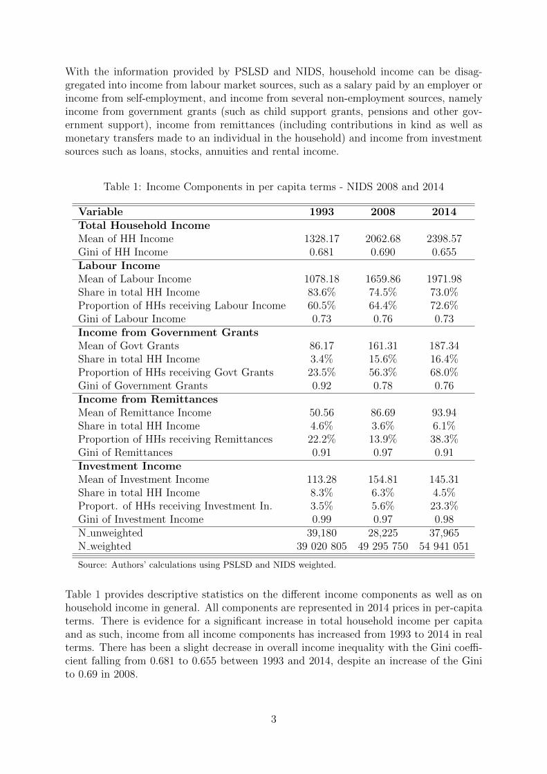
With the information provided by PSLSD and NIDS, household income can be disag-gregated into income from labour market sources, such as a salary paid by an employer orincome from self-employment, and income from several non-employment sources, namelyincome from government grants (such as child support grants, pensions and other gov-ernment support), income from remittances (including contributions in kind as well asmonetary transfers made to an individual in the household) and income from investmentsources such as loans, stocks, annuities and rental income.
Table 1: Income Components in per capita terms - NIDS 2008 and 2014
Variable 1993 2008 2014Total Household IncomeMean of HH Income 1328.17 2062.68 2398.57Gini of HH Income 0.681 0.690 0.655Labour IncomeMean of Labour Income 1078.18 1659.86 1971.98Share in total HH Income 83.6% 74.5% 73.0%Proportion of HHs receiving Labour Income 60.5% 64.4% 72.6%Gini of Labour Income 0.73 0.76 0.73Income from Government GrantsMean of Govt Grants 86.17 161.31 187.34Share in total HH Income 3.4% 15.6% 16.4%Proportion of HHs receiving Govt Grants 23.5% 56.3% 68.0%Gini of Government Grants 0.92 0.78 0.76Income from RemittancesMean of Remittance Income 50.56 86.69 93.94Share in total HH Income 4.6% 3.6% 6.1%Proportion of HHs receiving Remittances 22.2% 13.9% 38.3%Gini of Remittances 0.91 0.97 0.91Investment IncomeMean of Investment Income 113.28 154.81 145.31Share in total HH Income 8.3% 6.3% 4.5%Proport. of HHs receiving Investment In. 3.5% 5.6% 23.3%Gini of Investment Income 0.99 0.97 0.98N unweighted 39,180 28,225 37,965N weighted 39 020 805 49 295 750 54 941 051
Source: Authors’ calculations using PSLSD and NIDS weighted.
Table 1 provides descriptive statistics on the different income components as well as onhousehold income in general. All components are represented in 2014 prices in per-capitaterms. There is evidence for a significant increase in total household income per capitaand as such, income from all income components has increased from 1993 to 2014 in realterms. There has been a slight decrease in overall income inequality with the Gini coeffi-cient falling from 0.681 to 0.655 between 1993 and 2014, despite an increase of the Ginito 0.69 in 2008.
3
Labour income holds the largest share of total household income among the differentincome sources. A majority of households receive income from labour market sources andthe proportion of households receiving labour income has steadily increased from 60.5%in 1993 to 64% of all households in 2008 and 73% in 2014. The Gini coefficient for thiscomponent is relatively large and has fallen slightly by 0.032 points from 0.764 to 0.732between 2008 and 2014. Considering the strong dependency on this type on income, thisslight decrease in the Gini of income from labour market sources as well as the fact that,compared to 1993, much more households receive this type of income may be the driverof the overall decrease in income inequality within the observed time period. We returnto investigate this in more detail.
Interestingly, within the same time period, income from government grants has increasedas has the proportion of households receiving this type of income. The proportion ofhouseholds receiving some form of government support rose significantly from 23.5% in1993 to 56.3% in 2008 and as far as 68% in 2014. Income from government grants reportsa relatively large Gini coefficient which most likely stems from the fact that there aremany households reporting zero income from this source. Overall, the Gini of incomefrom government grants decreased slightly from 0.777 in 2008 to 0.758 in 2014. However,the Gini has fallen by 0.16 points since 1993 which is indicative of the fact that so manymore households receive grant income by 2014. Therefore, grant income plays a muchlarger role in total household income with its share having risen from only 6% in 1993 to16.4% in total household income by 2014.
In addition, the proportion of households receiving remittances has increased significantlybetween 1993 and 2014, despite a large drop in 2008. Previously, 22% of households re-ceived income in the form of inter-household transfers in cash and in kind. This proportiondropped to a low of 14% in 2008. In 2014, 38% of households received this form of income.There are less households reporting zero income from remittances, therefore, the distribu-tion of this type of income has become more equal. This would also explain the decreasefrom a Gini of 0.97 to 0.91 between 2008 and 2014. The overall share of remittances intotal household income is still relatively small and has increased between 1993 and 2014from 3.1% to 6.1% in total household income.
Lastly, we observe a strong increase in the proportion of households receiving incomefrom investment sources between 1993 and 2014. When previously only 3.5% of house-holds reported income from investment, 23% report this type of income in 2014. Invest-ment income remains highly unequal over the observed time period with a Gini coefficientclose to one in all three years. The fact that the share of investment in total householdincome has decreased, however, would indicate that other income components, namelylabour income and government grants, have grown stronger than investment income andplay a more important role in the income composition of the households.
Table 1 discussed the development of income in real terms in 1993, 2008 and 2014. In orderto interpret these changes, however, it is imperative to study changes in the underlyingdemographic variables as well. Thus, Table 2 presents descriptive statistics for householdcomposition variables. Household size has decreased from 4.38 in 1993 to 3.5 people inan average household in 2008 and then to 3.2 persons on average in 2014. Households
4
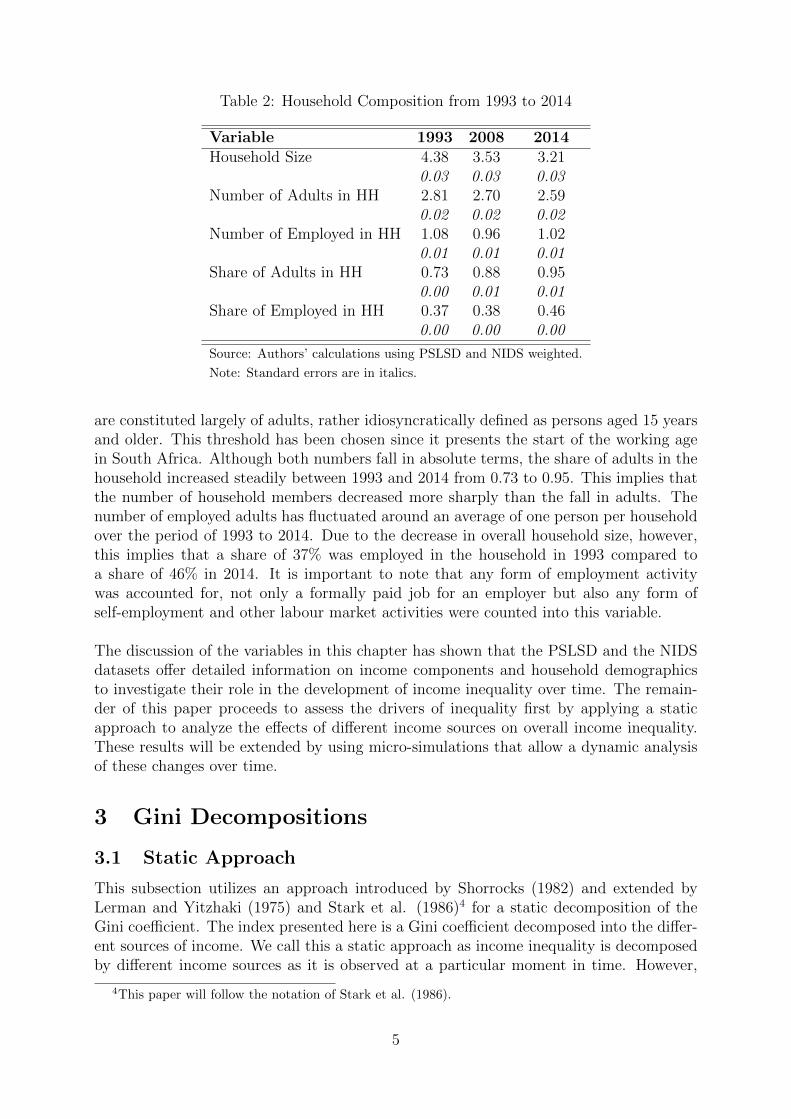
Table 2: Household Composition from 1993 to 2014
Variable 1993 2008 2014Household Size 4.38 3.53 3.21
0.03 0.03 0.03Number of Adults in HH 2.81 2.70 2.59
0.02 0.02 0.02Number of Employed in HH 1.08 0.96 1.02
0.01 0.01 0.01Share of Adults in HH 0.73 0.88 0.95
0.00 0.01 0.01Share of Employed in HH 0.37 0.38 0.46
0.00 0.00 0.00
Source: Authors’ calculations using PSLSD and NIDS weighted.
Note: Standard errors are in italics.
are constituted largely of adults, rather idiosyncratically defined as persons aged 15 yearsand older. This threshold has been chosen since it presents the start of the working agein South Africa. Although both numbers fall in absolute terms, the share of adults in thehousehold increased steadily between 1993 and 2014 from 0.73 to 0.95. This implies thatthe number of household members decreased more sharply than the fall in adults. Thenumber of employed adults has fluctuated around an average of one person per householdover the period of 1993 to 2014. Due to the decrease in overall household size, however,this implies that a share of 37% was employed in the household in 1993 compared toa share of 46% in 2014. It is important to note that any form of employment activitywas accounted for, not only a formally paid job for an employer but also any form ofself-employment and other labour market activities were counted into this variable.
The discussion of the variables in this chapter has shown that the PSLSD and the NIDSdatasets offer detailed information on income components and household demographicsto investigate their role in the development of income inequality over time. The remain-der of this paper proceeds to assess the drivers of inequality first by applying a staticapproach to analyze the effects of different income sources on overall income inequality.These results will be extended by using micro-simulations that allow a dynamic analysisof these changes over time.
3 Gini Decompositions
3.1 Static Approach
This subsection utilizes an approach introduced by Shorrocks (1982) and extended byLerman and Yitzhaki (1975) and Stark et al. (1986)4 for a static decomposition of theGini coefficient. The index presented here is a Gini coefficient decomposed into the differ-ent sources of income. We call this a static approach as income inequality is decomposedby different income sources as it is observed at a particular moment in time. However,
4This paper will follow the notation of Stark et al. (1986).
5
by taking the derivative with respect to a small percentage change in income from a par-ticular source, Stark et al. (1986) analyzed the effect of a marginal change in an incomesource on the overall Gini coefficient at that point in time holding all other income sourcesconstant. This section will briefly analyze the methodology of this static approach beforecomparing the decomposition of 1993 PSLSD data to NIDS 2008 and 2014.
The decomposition of the Gini coefficient is instrumental in analyzing the role of differentincome sources in more depth so as to gain a deeper understanding of the underlying fac-tors of South Africa’s persistently high levels of inequality. Following Stark et al. (1986),the overall Gini coefficient G0 can be presented as follows.
G0 =K∑k=1
Rk ·Gk · Sk (1)
where Sk and Gk are the share and the Gini coefficient of income component k respec-tively.5 Rk represents the so-called Gini correlation of component k with total householdincome, it shows similar characteristics as the Pearson’s and Spearman’s correlation co-efficients.
As such, equation (1) yields the decomposition of the Gini coefficient by income source(Stark et al., 1986). It allows us to examine three important concepts:
1. the share of the respective income source in overall household income, Sk
2. the inequality within the different income sources, Gk, and
3. the (Gini) correlation Rk between income component k and total household income.
By definition, the share of an income source in overall household income Sk and the Ginicoefficient of any income source Gk are always positive and bounded between 0 and 1.The Gini correlation Rk, however, will be positive when an income component contributespositively to the overall Gini, that is when yk is an increasing function of total income y0.Correspondingly, Rk will be negative when income component yk is a decreasing functionof total income y0. Rk is bounded by −1 ≤ Rk ≤ 1 and will be equal to zero when yk andy0 are uncorrelated.
In addition to the three concepts outlined above, the assessment of the effect of a smallchange in any one of the income components k on the overall Gini will be of interest. Forthis purpose, assume that an exogenous change in any income component j by a factor eoccurs. Then, income from j is assumed to change according to yj(e) = (1 + e)yj and
∂G0
∂e= Sj(Rj ·Gj −G0). (2)
Equation (2) is a partial derivative which simulates a marginal change in a particularincome source while holding income from other sources constant. Further, dividing (2)by G0 yields
∂G0/∂e
G0
=Sj ·Rj ·Gj
G0
− Sj. (3)
5The decomposition and the methodology are discussed in more detail in Appendix A.
6
Thus, the change in overall inequality due to a small change in income component j isequal to the initial share of j in total inequality less the share of component j in totalhousehold income (Stark et al., 1986). Given the characteristics of Rj, this yields twopossible outcomes for the overall Gini coefficient. If income component j has a negativeor zero correlation between j and total household income y0, an increase in income fromcomponent j will have an equalizing effect, thereby lowering inequality. This is due tothe fact that Sj, the share of income from component j, as well as the Gini indices for jand total income, Gj and G0, are always positive. The other possible outcome is when Rj
represents a positive Gini correlation. Assuming that Gj > G0, then Rk·Gk
Gwhich leads to
an increase in inequality associated with component j. Gj > G0 is a necessary conditionfor an inequality-increasing effect of income component j given that Rj is always smalleror equal to 1.
In summary, this approach allows us to analyze the three concepts laid out above aswell as the effect of a change in j on total income inequality. Nevertheless, the methodproposed by Stark et al. (1986) comes with one major limitation. When assessing thechange in one income component, income from all other components is held constant.However, the validity of this assumption is debatable as households tend to either com-pensate by increasing income from other sources or possibly decreasing efforts to obtainother income when income from one component j changes. As such, the approach byStark et al. (1986) provides a valuable snapshot of inequality within one period as wellas its decomposition but fails to adequately assess the effect of changes in income compo-nents on overall inequality. This is due to its one-dimensional approach which limits itspotential to analyze how changes in different income sources drive aggregate changes inincome inequality over a period of time.
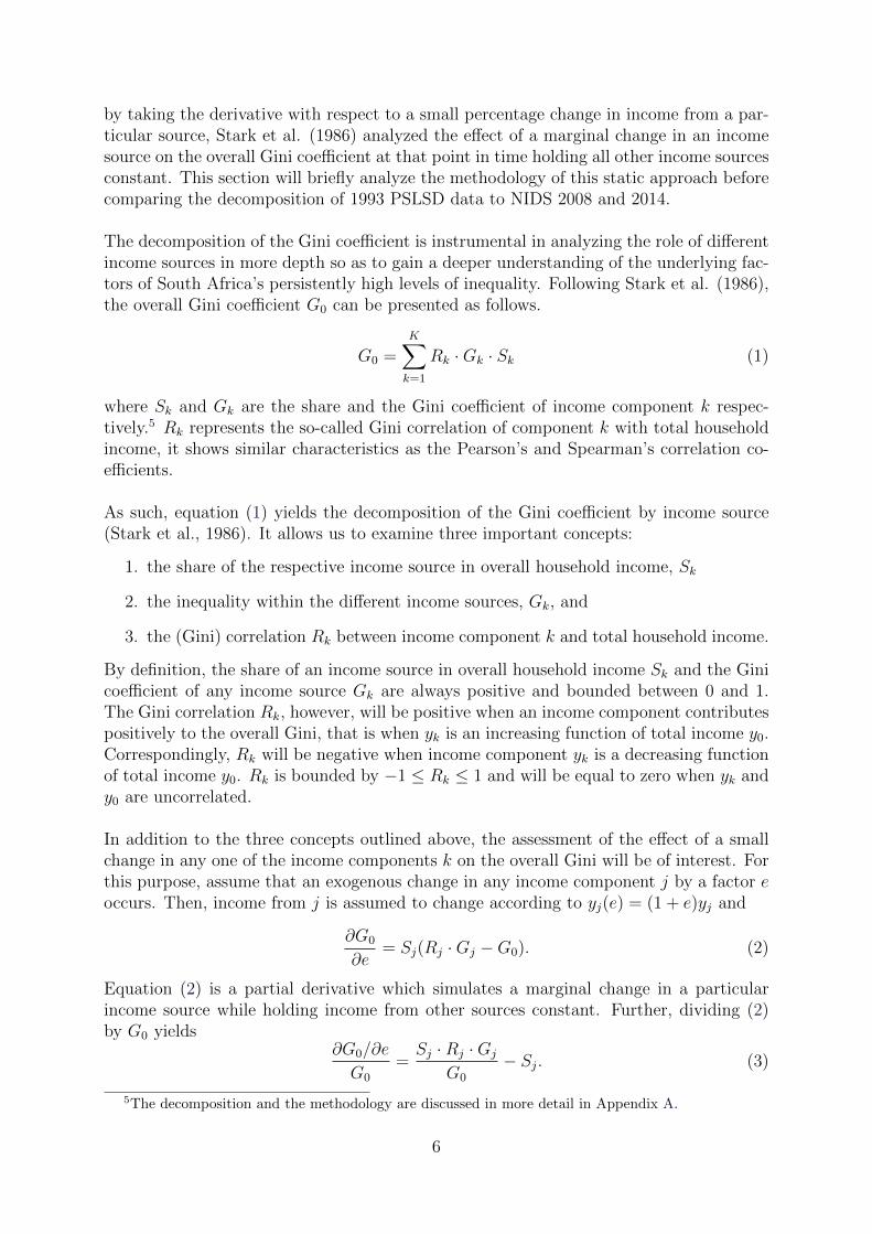
The results of the decomposition method by Stark et al. (1986) are provided in Ta-ble 3 for 1993, 2008 and 2014. Equation (1) has shown that the Gini coefficient is the sumof the products of the first three columns of Table 3 for each component k. These productsof SK · Rk · Gk are reported as the (absolute) contribution in column (4). The results inTable 3 show that income from labour market sources is the biggest driver of inequality.In 1993, labour income contributed 84.4% to overall inequality which increased to 87.2%in 2008 and 90.2% in 2014 as can be seen in Column (5) of Table 3 . The Gini coefficientof labour income was 0.73 in 1993, 0.759 in 2008 and 0.731 in 2014. Labour income isalso the most strongly correlated of all income sources with the Gini coefficient. The Ginicorrelation, or Rk is close to one for all three years under observation. In this context it isimportant to point out that the drop in the Gini of labour income between 2008 and 2014seems to have contributed to the large decrease in overall income inequality as measuredby the Gini coefficient. While the Gini of labour income decreased by 0.03 between 2008and 2014, the relative contribution increased by 3%. As labour is the largest contributorto overall inequality, the drop in the Gini of the income source explains partially whyoverall inequality has decreased. Most importantly, it is clear from the decompositionthat during the period under observation, labour income seems to be the driver behindhousehold income inequality.
The second largest driver of inequality is income from investment sources. This is de-spite the fact that between 1993 and 2014, the relative contribution of investment income
7
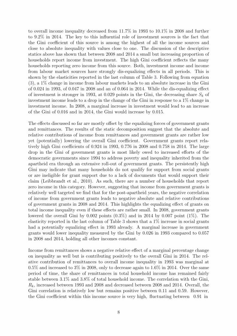
to overall income inequality decreased from 11.7% in 1993 to 10.1% in 2008 and furtherto 9.2% in 2014. The key to this influential role of investment sources is the fact thatthe Gini coefficient of this source is among the highest of all the income sources andclose to absolute inequality with values close to one. The discussion of the descriptivestatics above has shown that between 2008 and 2014 a small but increasing proportion ofhouseholds report income from investment. The high Gini coefficient reflects the manyhouseholds reporting zero income from this source. Both, investment income and incomefrom labour market sources have strongly dis-equalizing effects in all periods. This isshown by the elasticities reported in the last column of Table 3. Following from equation(3), a 1% change in income from labour markets leads to an absolute increase in the Giniof 0.024 in 1993, of 0.047 in 2008 and an of 0.064 in 2014. While the dis-equalizing effectof investment is stronger in 1993, at 0.029 points in the Gini, the decreasing share Sk ofinvestment income leads to a drop in the change of the Gini in response to a 1% change ininvestment income. In 2008, a marginal increase in investment would lead to an increaseof the Gini of 0.016 and in 2014, the Gini would increase by 0.015.
The effects discussed so far are mostly offset by the equalizing forces of government grantsand remittances. The results of the static decomposition suggest that the absolute andrelative contributions of income from remittances and government grants are rather lowyet (potentially) lowering the overall Gini coefficient. Government grants report rela-tively high Gini coefficients of 0.924 in 1993, 0.776 in 2008 and 0.758 in 2014. The largedrop in the Gini of government grants is most likely owed to increased efforts of thedemocratic governments since 1994 to address poverty and inequality inherited from theapartheid era through an extensive roll-out of government grants. The persistently highGini may indicate that many households do not qualify for support from social grantsor are ineligible for grant support due to a lack of documents that would support theirclaim (Leibbrandt et al., 2010). As such, there are a number of households that reportzero income in this category. However, suggesting that income from government grants isrelatively well targeted we find that for the post-apartheid years, the negative correlationof income from government grants leads to negative absolute and relative contributionsof government grants in 2008 and 2014. This highlights the equalizing effect of grants ontotal income inequality even if these effects are rather small. In 2008, government grantslowered the overall Gini by 0.002 points (0.3%) and in 2014 by 0.007 point (1%). Theelasticity reported in the last column of Table 3 shows that a 1% increase in social grantshad a potentially equalizing effect in 1993 already. A marginal increase in governmentgrants would lower inequality measured by the Gini by 0.026 in 1993 compared to 0.057in 2008 and 2014, holding all other incomes constant.
Income from remittances shows a negative relative effect of a marginal percentage changeon inequality as well but is contributing positively to the overall Gini in 2014. The rel-ative contribution of remittances to overall income inequality in 1993 was marginal at0.5% and increased to 3% in 2008, only to decrease again to 1.6% in 2014. Over the sameperiod of time, the share of remittances in total household income has remained fairlystable between 3.1% and 3.8% of total household income. The correlation with the Gini,Rk, increased between 1993 and 2008 and decreased between 2008 and 2014. Overall, theGini correlation is relatively low but remains positive between 0.11 and 0.59. However,the Gini coefficient within this income source is very high, fluctuating between 0.91 in
8
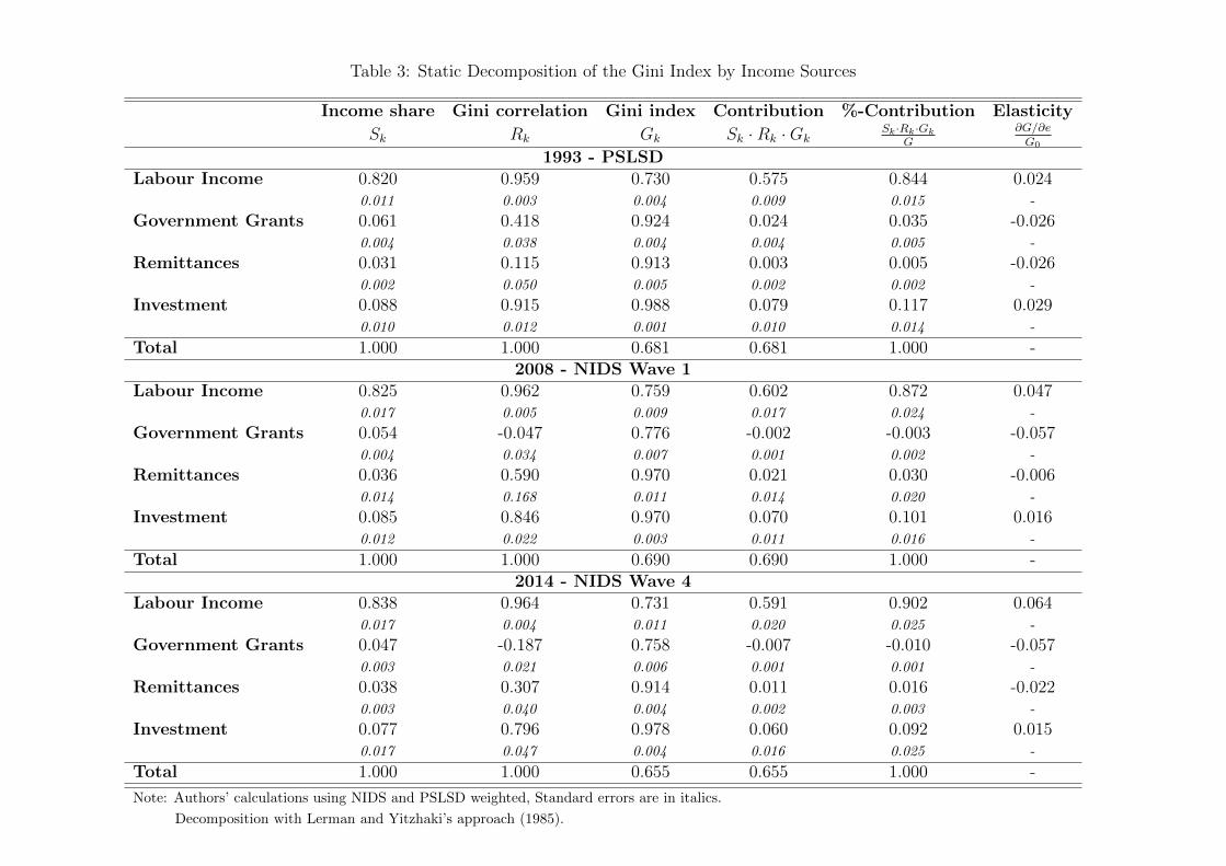
Table 3: Static Decomposition of the Gini Index by Income Sources
Income share Gini correlation Gini index Contribution %-Contribution Elasticity
Sk Rk Gk Sk ·Rk ·GkSk·Rk·Gk
G∂G/∂eG0
1993 - PSLSDLabour Income 0.820 0.959 0.730 0.575 0.844 0.024
0.011 0.003 0.004 0.009 0.015 -
Government Grants 0.061 0.418 0.924 0.024 0.035 -0.0260.004 0.038 0.004 0.004 0.005 -
Remittances 0.031 0.115 0.913 0.003 0.005 -0.0260.002 0.050 0.005 0.002 0.002 -
Investment 0.088 0.915 0.988 0.079 0.117 0.0290.010 0.012 0.001 0.010 0.014 -
Total 1.000 1.000 0.681 0.681 1.000 -2008 - NIDS Wave 1
Labour Income 0.825 0.962 0.759 0.602 0.872 0.0470.017 0.005 0.009 0.017 0.024 -
Government Grants 0.054 -0.047 0.776 -0.002 -0.003 -0.0570.004 0.034 0.007 0.001 0.002 -
Remittances 0.036 0.590 0.970 0.021 0.030 -0.0060.014 0.168 0.011 0.014 0.020 -
Investment 0.085 0.846 0.970 0.070 0.101 0.0160.012 0.022 0.003 0.011 0.016 -
Total 1.000 1.000 0.690 0.690 1.000 -2014 - NIDS Wave 4
Labour Income 0.838 0.964 0.731 0.591 0.902 0.0640.017 0.004 0.011 0.020 0.025 -
Government Grants 0.047 -0.187 0.758 -0.007 -0.010 -0.0570.003 0.021 0.006 0.001 0.001 -
Remittances 0.038 0.307 0.914 0.011 0.016 -0.0220.003 0.040 0.004 0.002 0.003 -
Investment 0.077 0.796 0.978 0.060 0.092 0.0150.017 0.047 0.004 0.016 0.025 -
Total 1.000 1.000 0.655 0.655 1.000 -
Note: Authors’ calculations using NIDS and PSLSD weighted, Standard errors are in italics.
Decomposition with Lerman and Yitzhaki’s approach (1985).
1993 and 2014 and 0.97 in 2008. This is due to the fact that many households report zeroincome in this income category which drives up the Gini coefficient within the incomesource. The marginal change analysis show that remittances have potential to lower theGini coefficient. A 1% increase in remittances would lead to a 0.026 decrease in inequalityas measured by the Gini in 1993, a decrease of 0.006 in 2008 and a decrease of the Gini by0.022 in 2014. Thus, the elasticities reveal a stronger redistributive effect of this incomesource than the static decomposition alone.
The main shortcoming of the approach proposed by Stark et al. (1986) is in its staticanalysis. While this decomposition allows a detailed analysis of the contribution of differ-ent income sources in a given year, it is limited in its evaluation of the effect of changes inone income source on changes in total inequality. The elasticities measured here are giventhat all other household decisions regarding income are held constant which remains aquestionable assumption. For example, if the arrival of a state old age pension pushes ahousehold up the income distribution, the decomposition reflects the situation after thearrival of the pension. The elasticities are an attempt to correct for this weakness. How-ever, they can only simulate a small or marginal change in income from a source, holdingall other sources constant. Thus, the estimated elasticities are limited as simulations ofthe influence on the income distribution of sources that changed quite markedly over thepost-apartheid period. To overcome this, we proceed to a more contemporary approachthat uses micro-simulations to assess the effect of changes in one income source on overallinequality.
3.2 Micro Simulations
Even though the static decomposition offers a useful snapshot of inequality from a cross-sectional point of view, it only provides limited insights in the effects of changes in eachincome source to changing inequality. We therefore introduce an approach by Barroset al. (2006) and Azevedo et al. (2013) that tries to model changes in different incomesources using micro-simulations. The following section will be implementing this so-calleddynamic decomposition of income inequality.
Following Azevedo et al. (2013), the micro-simulations used in his approach model coun-terfactuals by changing one factor at a time in order to decompose the contribution ofthe effect of measured changes in the different income sources. An additional strength tothese dynamic decompositions is that it facilitates the modeling of changes in income percapita and, therefore, a focus on changes in the denominator allows us to examine andseparate out the impact of changes in household demographics.
Following the notation of Azevedo et al. (2013), household income per capita can berepresented as the sum of incomes of all household members over the number of house-hold members n.
Ypc =Yhn
=1
n
n∑i=1
yi, (4)
where yi is the income of individual i and Yh is the total household income. Equation(4) can be rewritten assuming that only persons aged 15 years and above are able tocontribute to household income. Then, in fact, household income per capita will depend
10
on the number of adults in the household or nA such that
Ypc =nA
n
(1
nA
n∑i∈A
yi
), (5)
where nA
nrepresents the share of adults in the household. The expression in parentheses
is the income per adult which can be written as the sum of income from different incomesources. Assume for simplicity that income per adult can be divided into two sub cat-egories, labour income and income from non-labour sources or yLi and yNL
i respectively(Azevedo et al., 2013). In the context of this paper, income from non-labour sources mayinclude income from social grants, pensions and other government sources, remittances orinvestment income. Regarding labour income, it is important to note that not all adultsin the household will be employed, instead only the share n0
nAwill earn income from labour
markets with n0 being the number of employed adults. Then, equation (5) transformsinto
Ypc =nA
n
(1
nA
n∑i∈A
yLi +1
nA
n∑i∈A
yNLi
)(6)
=nA
n
[n0
nA
(1
n0
n∑i∈A
yLi
)+
1
nA
n∑i∈A
yNLi
]. (7)
The distribution of household per capita income F (·) depends on the different componentsoutlined in equation (7) and in turn, inequality measures depend on the cumulative densityfunction F (·) and as such, can be written as a function of the components discussed above.
Azevedo et al. (2013) show that micro simulations can be used to estimate the contribu-tion of each component to the observed changes in the inequality measures by changingeach component one at a time. With this in mind, assume that ϑ is a measure of inequal-ity and as such a function of the cumulative density function F (·) and the componentsoutlined above. Then
ϑ = Φ(F (Ypc(n,nA
n,n0
nA
,1
n0
n∑i∈A
yLi︸ ︷︷ ︸yLP0
,1
nA
n∑i∈A
yNLi︸ ︷︷ ︸
yNLPA
))), (8)
with yLP0 representing labour market incomes and yNLPA being the non-labour income in-
cluding government grants, remittances and investment income. In order to estimate thecontribution of each component to the observed changes in the inequality between period1 and period 2, Azevedo et al. (2013) substitute the period 1 level of the respectiveincome source into the counterfactual distribution of period 2. To give an illustrationfor the case of the study at hand, assume there is a change in the share of adults in ahousehold between 1993 and 2008. Following Azevedo et al. (2013), the counterfactualswill be created by ordering households according to their household income per capitaand then averaging the values of each component in equation (8) by quantiles. In orderto compute ϑ, the 1993 value of n0
nAwill be substituted into the distribution of income
f(·) by quantiles observed in 2008:
ϑ = Φ(F (Ypc(n,nA
n,n0
nA
, yLP0, yNLPA))). (9)
11
Then, ϑ− ϑ is the estimated contribution of the share of adults that earn labour marketincome in 2008. In the same manner in which n0
nAwas substituted, each of the other com-
ponents of interest can be substituted into the distribution of income per capita in 2008following the rank-preserving exercise and their contribution to changes in inequality canbe estimated. For example, when decomposing the impact of labour market incomes, the2008 labour market income will be substituted with the average labour market income in1993 for each quantile. The effect of labour market income on inequality is then measuredby comparing the level of inequality of the simulated data with actual levels of inequalityobserved in 2008.
Azevedo et al. (2013) refine the method introduced by Barros et al. (2006) by com-puting what they call a “cumulative counterfactual distribution”. By adding one variableat a time, the impacts of a change in each of the variables of interest and their interactionscan be estimated as the difference between those cumulative counterfactuals (Azevedo etal., 2013).
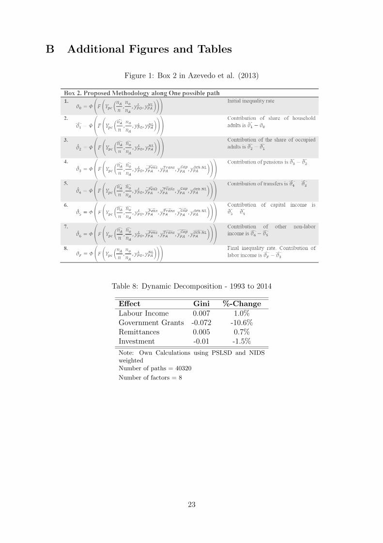
One technical issue that has to be addressed in the simulation is the fact that the cu-mulative counterfactuals estimated differ depending on the order in which the differentvariables are added. In other words, the path that is used for the estimation of the cu-mulative effects matters. This problem is called path-dependence (Azevedo et al., 2013).In order to overcome this caveat, Azevedo et al. (2013) suggest calculating the Shapley-Shorrocks estimate of each component. The Shapley-Shorrocks estimate calculates thedecomposition across all possible paths before averaging the results.6 Since there areeight variables of interest, this aggregates to 40, 320 possible paths, i.e. the result of 8factorial. The estimates of the Shapeley-Shorrocks values are reported in the tables below.
While this prevents the analysis from suffering from this major shortcoming, one caveatremains. The counterfactuals calculated in this manner are the result of a statistical ex-ercise rather than actual economic equilibria, in which it is assumed that one componentcan be changed at a time, keeping all other factors constant. However, an increase in anyincome source would generally lead to an adjustment in economic behaviour. Householdstend to substitute a loss in one income source with an increase in another and, vice versa,an increase in one income source may cause a decrease in efforts to obtain income fromanother source. Nevertheless, since the Shapeley-Shorrocks values calculate the averagesof this substituting exercise, they represent the closest possible approximation. Therefore,we proceed to calculate these simulated counterfactuals using the 1993 PSLSD and NIDS2008 and 2014 data sets.
The decompositions are done in two steps, first from 1993 to 2008, then from 2008 to2014. The dynamic decomposition will be broken into these two steps since the results ofthe static decomposition exercises showed that there was an increase in inequality between1993 and 2008, whereas the static decomposition reported a decrease between 2008 and2014. In the dynamic decomposition, we would like to assess what drove the increase andlater decrease of inequality over these periods of time.7
6For details of this cumulative path method, see Box 2 from Azevedo et al. (2013) in Appendix B.7The results of the dynamic decomposition from 1993 to 2014 are reported in Appendix B.
12

Table 4: Dynamic Decomposition - 1993 to 2008
Effect Gini %-ChangeLabour Income 0.029 4.3%Government Grants -0.063 -9.3%Remittances 0.018 2.6%Investment -0.002 -0.3%
Note: Own Calculations using PSLSD and NIDSweightedNumber of paths = 40320
Number of factors = 8
Before we can proceed and compare the PSLSD and NIDS data sets in this dynamicdecomposition, it is necessary to undertake a rank-preserving exercise as discussed above.Following Azevedo et al. (2013), households will be ranked by income per capita anddivided into quantiles. For each of those quantiles, the average of each component inequation (8) in the first period, say 1993, will be assigned to each household in the samequantile in the second period, say 2008. This will be done for households ranked accord-ing to their household income per capita, however, it is possible to order households bythe different income components instead. This may offer some insights into the effectsof changes in that particular component on overall inequality. For components that arehighly correlated with overall inequality, this change in the ranking order will result insmall differences. However, when this is not the case, re-ranking according to differentincome sources allows us to differentiate shifts in the overall income distributions fromdevelopments within the distribution of the particular income source.
Table 5: Dynamic Decomposition - 2008 to 2014
Effect Gini %-ChangeLabour Income -0.021 -3.0%Government Grants -0.012 -1.7%Remittances -0.012 -1.7%Investment -0.006 -0.9%
Note: Own Calculations using NIDS W1 and W4weightedNumber of paths = 40320
Number of factors = 8
To sum up, Tables 6 and 7 will provide the results of the simulations following differentrankings. The decomposition in Tables 4 and 5 ranks households according to overall percapita income. It reports the estimation without taking account of changes in demogra-phy. It is therefore implicitly attributing these demographic to changes in the per capitavalues of the different income sources. As such, the results in Tables 4 and 5 serve asbenchmarks for further analysis.
13
The estimation in Table 4 shows that between 1993 and 2008, changes in labour incomehad an increasing effect on the Gini which is similar to the results found in the staticdecomposition. In the observed time period, changes in labour income increased the Giniby 0.029 points or 4.3% of the original Gini. Changes in incomes from non-labour sources,on the other hand, mostly had an equalizing effect, lowering the overall Gini coefficient.The strongest effect is from government grants. Changes in government grants loweredthe Gini by 0.063 points (9.3%). This reflects the substantial roll out of social grants and,in particular, the Child Support Grant that is documented in Leibbrandt et al. (2010).Changes in income from investment also had an overall negative effect on the Gini of0.002 points or 0.3%. This is most likely due to the fact that the share of income frominvestment sources fell sharply in the period observed while the proportion of householdsreceiving this type of income increased. Income from remittances increased the Gini by0.018 points which translates into a 2.6% change from the 1993 Gini coefficient. If werecall Table 1 that reported on descriptive statistics of the different income sources, we seethat the share of remittances in total income as well as the share of households receivingincome from this source decreased between 1993 and 2008. This can help explain howremittances contributed to an increase in inequality between 1993 and 2008.
Turning now to the 2008 to 2014 period, from the static decomposition we know thatbetween 2008 and 2014 the overall Gini coefficient decrease from 0.69 to 0.655. The dy-namic decomposition using NIDS 2008 and 2014 data shows that all income componentscontributed to this fall in overall inequality. Again, we used a rank preserving and demog-raphy preserving exercise to compare households in 2008 with 2014. Results are reportedin Table 5. The strongest contributor to the decline in overall inequality was income fromlabour market sources. Changes in income from labour markets resulted in a decreasein the Gini of 0.021 or 3%. This supports the results of the static decomposition whichshowed that the Gini within labour market income had fallen but the contribution to theoverall Gini had increased. As such, a decrease in inequality from labour market incomemay have driven the overall decrease in inequality. However, labour market income wasnot the only contributor to a decrease in total household income inequality. Changes inincomes from government grants as well as remittances each resulted in a decrease in theGini of 1.7%. Furthermore, changes in investment income decreased the Gini coefficientby another 0.9%.
The approach developed by Azevedo et al. (2013) allows us to differentiate the changesin inequality not only according to different income sources but also by household demo-graphics. In Table 2, we presented a basic description of household demographics at eachof the three points in time. To recapitulate, household size decreased between 1993 and2014 from an average of 4.4 persons in a household to only 3.2 on average. At the sametime, the share of adults as well as the share of employed household members increased.In 1993, 73.4% of the household were 15 or above compared to 95.4% in 2014 and theshare of employed had increased from 37% to 46%. Tables 6 and 7 go on to factor inthese changes in household decomposition into the dynamic decompositions. The tablesalso allow for a re-ranking of income sources.
It can be seen from Table 6 that between 1993 and 2008 the change in the share ofadults in the household increased the Gini coefficient by 0.002 units (0.3%). The share
14
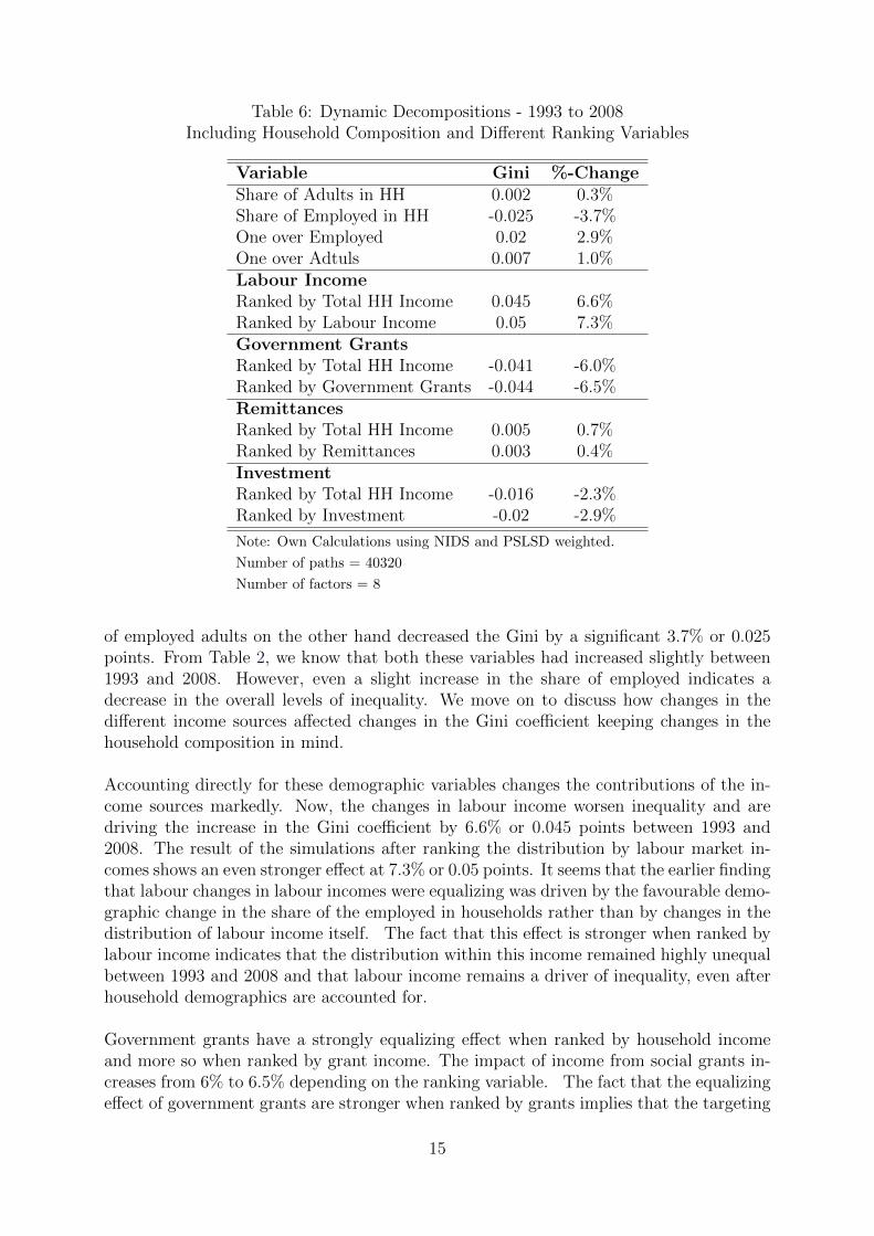
Table 6: Dynamic Decompositions - 1993 to 2008Including Household Composition and Different Ranking Variables
Variable Gini %-ChangeShare of Adults in HH 0.002 0.3%Share of Employed in HH -0.025 -3.7%One over Employed 0.02 2.9%One over Adtuls 0.007 1.0%Labour IncomeRanked by Total HH Income 0.045 6.6%Ranked by Labour Income 0.05 7.3%Government GrantsRanked by Total HH Income -0.041 -6.0%Ranked by Government Grants -0.044 -6.5%RemittancesRanked by Total HH Income 0.005 0.7%Ranked by Remittances 0.003 0.4%InvestmentRanked by Total HH Income -0.016 -2.3%Ranked by Investment -0.02 -2.9%
Note: Own Calculations using NIDS and PSLSD weighted.
Number of paths = 40320
Number of factors = 8
of employed adults on the other hand decreased the Gini by a significant 3.7% or 0.025points. From Table 2, we know that both these variables had increased slightly between1993 and 2008. However, even a slight increase in the share of employed indicates adecrease in the overall levels of inequality. We move on to discuss how changes in thedifferent income sources affected changes in the Gini coefficient keeping changes in thehousehold composition in mind.
Accounting directly for these demographic variables changes the contributions of the in-come sources markedly. Now, the changes in labour income worsen inequality and aredriving the increase in the Gini coefficient by 6.6% or 0.045 points between 1993 and2008. The result of the simulations after ranking the distribution by labour market in-comes shows an even stronger effect at 7.3% or 0.05 points. It seems that the earlier findingthat labour changes in labour incomes were equalizing was driven by the favourable demo-graphic change in the share of the employed in households rather than by changes in thedistribution of labour income itself. The fact that this effect is stronger when ranked bylabour income indicates that the distribution within this income remained highly unequalbetween 1993 and 2008 and that labour income remains a driver of inequality, even afterhousehold demographics are accounted for.
Government grants have a strongly equalizing effect when ranked by household incomeand more so when ranked by grant income. The impact of income from social grants in-creases from 6% to 6.5% depending on the ranking variable. The fact that the equalizingeffect of government grants are stronger when ranked by grants implies that the targeting
15
of grants was effective in addressing households at the bottom of the income distribution.Compared to the baseline results of Table 4, the effect of government grants is lower oncedemographic changes are separated out. This highlights the necessity to account for thesedemographic variables.
Changes in remittances increased inequality, both when ranked by total household in-come as well as ranked by remittance income. The effect is small at 0.7% in the first caseand decreases to 0.4% in the latter. Remittances probably have such a small effect on theGini due to the fact that they play only a minor role in overall household income. Theresults of the static decomposition in Table 3 showed that remittances only contributedbetween 0.5% and 3% to total inequality and their shares in income were at about 3%.When we asses the effect of remittances and rank by remittance income, we find that theeffect is smaller than when ranked by total household income. This indicates that thedistribution of remittances is slightly more equal than the distribution overall householdincome. It supports the findings of the static decomposition that highlighted the equal-izing potential of remittances even though they were contributing positively to overallinequality.
Finally, changes in income from investment sources had a small but equalizing effecton changes in the Gini for the different rankings. When ranked by total income, thiseffect is at 2.3%. When assessing the effect of changes in the distribution of investmentincome, the effect is at 2.9%. These effects are much larger than the 0.3% estimated inthe benchmark case which highlights the importance of separating out the role of changesin household composition.
Overall, it would seem that increased efforts by the post-Apartheid state in addressingpoverty and inequality through government grants have largely offset inequality increasingeffects of labour market income. Government grants reduced inequality significantly butnot enough so that overall inequality increased between 1993 and 2008, driven predom-inantly by changes in inequality from labour market incomes. Table 7 will now analysethe drivers of changes in inequality between 2008 and 2014.
We start with demographic changes. Both the share of adults as well as the share ofemployed adults in a household had an increasing effect on inequality between 2008 and2014. The effects are significant at about 1% of the 2008 Gini in both cases. This isinteresting as both shares have increased between 2008 and 2014 (see Table 1). The sharehad increased previously, however, between 1993 and 2008 the share of employed had ledto a decrease in the Gini. In order to harmonize these results, we move on to analyzingthe effects of changes in the different income sources.
Once these demographic variables are accounted for, income from all sources contributedto the decline in overall inequality. The strongest driver in the fall of the Gini coeffi-cient is income from labour market sources. The effect is at -0.046 points of the Gini or-6.7%. This large change is the same when ranked by total household income as whenranked by labour income. This supports the very strong correlation found between labourincome and total household income per capita in the static decomposition. In Table 1we reported that the share of labour income dropped between 2008 and 2014 while the
16
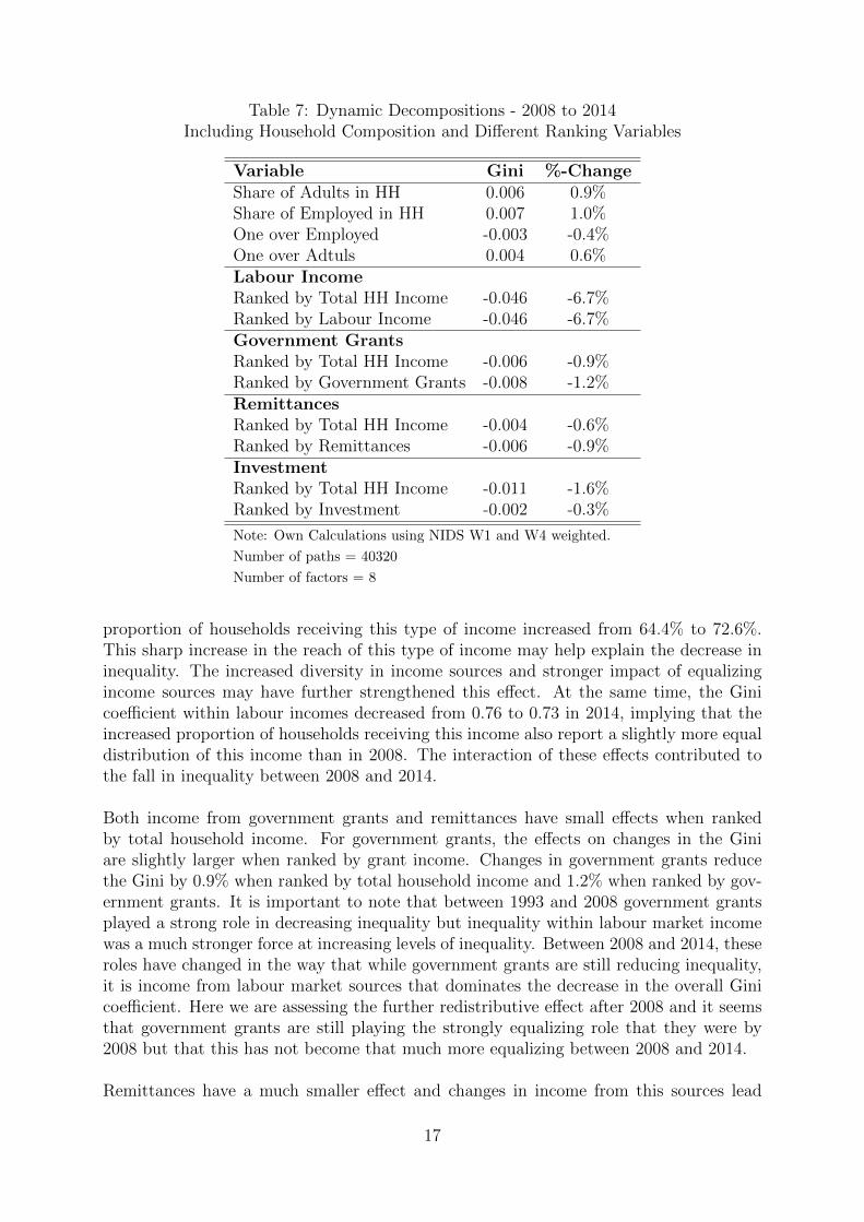
Table 7: Dynamic Decompositions - 2008 to 2014Including Household Composition and Different Ranking Variables
Variable Gini %-ChangeShare of Adults in HH 0.006 0.9%Share of Employed in HH 0.007 1.0%One over Employed -0.003 -0.4%One over Adtuls 0.004 0.6%Labour IncomeRanked by Total HH Income -0.046 -6.7%Ranked by Labour Income -0.046 -6.7%Government GrantsRanked by Total HH Income -0.006 -0.9%Ranked by Government Grants -0.008 -1.2%RemittancesRanked by Total HH Income -0.004 -0.6%Ranked by Remittances -0.006 -0.9%InvestmentRanked by Total HH Income -0.011 -1.6%Ranked by Investment -0.002 -0.3%
Note: Own Calculations using NIDS W1 and W4 weighted.
Number of paths = 40320
Number of factors = 8
proportion of households receiving this type of income increased from 64.4% to 72.6%.This sharp increase in the reach of this type of income may help explain the decrease ininequality. The increased diversity in income sources and stronger impact of equalizingincome sources may have further strengthened this effect. At the same time, the Ginicoefficient within labour incomes decreased from 0.76 to 0.73 in 2014, implying that theincreased proportion of households receiving this income also report a slightly more equaldistribution of this income than in 2008. The interaction of these effects contributed tothe fall in inequality between 2008 and 2014.
Both income from government grants and remittances have small effects when rankedby total household income. For government grants, the effects on changes in the Giniare slightly larger when ranked by grant income. Changes in government grants reducethe Gini by 0.9% when ranked by total household income and 1.2% when ranked by gov-ernment grants. It is important to note that between 1993 and 2008 government grantsplayed a strong role in decreasing inequality but inequality within labour market incomewas a much stronger force at increasing levels of inequality. Between 2008 and 2014, theseroles have changed in the way that while government grants are still reducing inequality,it is income from labour market sources that dominates the decrease in the overall Ginicoefficient. Here we are assessing the further redistributive effect after 2008 and it seemsthat government grants are still playing the strongly equalizing role that they were by2008 but that this has not become that much more equalizing between 2008 and 2014.
Remittances have a much smaller effect and changes in income from this sources lead
17
to a 0.6% decrease in the overall Gini when ranked by total household income. Thiseffect is slightly stronger when ranked by remittance income at 0.9%. This supports thepotential to decrease inequality that we discussed in the static decomposition. However,the static decomposition reported that remittances are currently contributing to inequal-ity. The dynamics decompositions shows that when the effects of household compositionvariables are netted out, remittances decrease inequality between 2008 and 2014.
Finally, income from investment sources has a decreasing effect on the Gini as well. In-terestingly, the effect is lower when ranked by investment income at only 0.3%. Rankedby total household income, changes in investment result in a 1.6% change in the Gini.The fact that the changes in the Gini are smaller when ranked by investment income mayindicate that the distribution of income from this source is still rather unequal and onlysmall changes occurred between 2008 and 2014.
In Appendix B, Tables 8 and 9 report the aggregate trends from a broad-period decom-position that applies the different methods of Azevedo et al. (2013) to compare changesbetween 1993 and 2014. In this long-term comparison we find that the effect of govern-ment grants on changes in the Gini is very strong (-10.6%) in the baseline decomposition.Table 8 which does not account for household demographics finds that changes in labourincome contributed 1.0% to the overall changes in inequality measured by the Gini andthat remittances contributed 0.7%. Investment income decreased the Gini coefficient by0.01 units or 1.5% between 1993 and 2014. Once we account for household compositionvariables, these effects change slightly.
The results reported in Table 9 show that the share of adults in a household contribute toa 1.3% change in the Gini coefficient between 1993 and 2014, this is equivalent to 0.009units. The share of employed adults in a household lead to a 2.9% decrease over the sametime period. However, it is important to note that the separated decomposition of Table6 and Table 7 reported that the share of employed had a decreasing effect of close to4% only between 1993 and 2008, whereas between 2008 and 2014 changes in the share ofemployed contributed to a 1% increase in the Gini.
Table 9 also reports that over the period of 1993 to 2014 changes in labour income con-tributed to a 0.6% decrease in the Gini when ranked by total household income. Whenthis is ranked by labour income, however, the effect reverses and it reports an increase inthe Gini by 0.6%. The fact that the change in the Gini is negative when ranked by totalhousehold income and positive when ranked by labour income would indicate a slightlymore unequal distribution within labour market income. It fails to decompose the in-equality increasing effect of labour income that we found between 1993 and 2008 and theinequality reducing effect between 2008 and 2014.
Furthermore, between 1993 and 2014, changes in government grants reduced the Giniby 6.3%, 7% when ranked by grant income. This is in line with the inequality reducingeffects we found previously and seems to be the aggregate of the effects we found between1993 and 2008 and between 2008 and 2014 respectively. The effect of remittances overthe entire time period netted out to zero when ranked by total household income anda small -0.3% when ranked by remittance income. While this appears to be the aggre-
18
gate of the separate effects found in Tables 6 and 7, this overall analysis fails to uncoverthe inequality increasing effects of remittances between 1993 and 2008 that were offsetby the inequality decreasing effect of changes in this income source between 2008 and 2014.
Finally, investment was found to have a decreasing effect of 4.6% when ranked by totalhousehold income and reports a slightly smaller effect of 2.3% when ranked by investmentincome. It should have become clear that while the decomposition between 1993 and2014 generally reports the aggregated trends in inequality over the observed time period,it fails to account for changes in the effects of the different income source on the increaseand then decrease of overall inequality measured by the Gini coefficient uncovered by theseparate decompositions.
The above decompositions of changes in inequality between 1993 and 2008 as well as2008 and 2014 respectively, show that government grants are strong drivers in the reduc-tion of overall income inequality. Furthermore, changes in labour market income havestrong effects on overall inequality measured by the Gini coefficient. Between 1993 and2008, it was income from labour markets that drove the increase in inequality and between2008 and 2014, income from this source contributed strongly to a decrease in the Gini.The equalizing role of government grants has long been established in the literature (seeLeibbrandt et al., 2012, and Leibbrandt et al., 2010) and as such, the ambivalent effectof changes in the labour income are left to be explored in more detail in future research.
4 Conclusion
This paper has applied different decomposition methods in order to ascertain drivers ofinequality in South Africa over the post-apartheid period. A static decomposition by in-come sources highlighted the dominance of contributions in labour market income. Usingdata from the Project for Statistics on Living Standards and Development from 1993 aswell as from the National Income Dynamics Study from 2008 and 2014, labour marketincome has been shown to be the largest contributor to the high levels of inequality inSouth Africa. Furthermore, we have shown that while inequality was rising from 0.68in 1993 to about 0.7 in 2008, it has been declining in recent years to a Gini coefficientof 0.655 by 2014. According to the decompositions performed in this paper, householdsbenefit significantly from income from government grants, however, labour income as wellas investment income strongly contribute to overall inequality.
The different methods of decomposing inequality according to income sources have shownthat income from labour markets is a strong driver behind high inequality levels in SouthAfrica. The static decomposition method following Stark et al. (1986) suggested thatlabour market income contributes between 84% and 90% to the overall Gini coefficientsbetween 1993 and 2014, proceeded by large contributions of investment income to in-equality. We also find that between 2008 and 2014, labour market incomes remain highlycorrelated with overall inequality. The dynamic decomposition has shown that between1993 and 2008 it was income from labour markets that dominated the increase in inequal-ity and that changes in inequality within labour market income contributed strongly tothe decrease on inequality between 2008 and 2014.
19
The dynamic approach following Azevedo et al. (2013) implements a series of counter-factual simulations to identify the direct effect of a change in a particular income sourceon the total income inequality. The results of the different ranking exercises within thedynamic decomposition showed that changes in the targeting and extensions to the sys-tem of government grants largely offset the inequality increasing effects of labour incomebetween 1993 and 2008. The static decomposition method was unable to differentiatebetween the effects of labour income and government grants in that way. The role ofgovernment grants changed hugely between 1993 and 2008. Poverty-alleviating policiesthat resulted in an increase in government grants limited the increase in inequality overthis period immensely. Even between 2008 and 2014, government grants played a sig-nificant role in reducing inequality and different ranking methods show that targeting ofsocial policies was successful in addressing those households at the bottom of the incomedistribution.
Furthermore, the dynamic approach has shown that investment income played a muchsmaller yet inequality reducing role, particularly between 1993 and 2008. The staticdecomposition failed to detect these lowering effects of investment income on inequality.Additionally, the results of the static decomposition suggested that while remittances havethe potential to lower inequality, as shown by negative elasticities, they are contributingpositively to inequality. However, the dynamic approach using micro simulations paints adifferent picture. Once we account for demographic changes, remittances led to increasesin the Gini between 1998 and 2008 but helped decrease inequality between 2008 and 2014.Aggregated across both time periods, however, the effects of remittances were close to zero.
The more nuanced analysis using micro-simulations allowed us to account for changesin household demographics as well as changes in income sources. Changes in the shareof employed adults had a dis-equalizing effect between 1993 and 2008 but an equalizingeffect between 2008 and 2014, whereas changes in the number of adults in a householdled to an increase in the Gini in both periods. The effects of both these variables wouldbe overlooked in the decomposition method by Stark et al. (1986). Particularly between2008 and 2014 we find that it is the household composition variables that drive inequal-ity upwards, whereas all income sources report an equalizing effect. This highlights theimprovement in information by using the method of Azevedo et al. (2013).
All in all, this paper analyzed the development of inequality over the past 20 years us-ing household survey data, showing that inequality has started to fall in South Africa.However, the static and dynamic analysis in this paper highlight the need for further im-provement especially with regards to the high level of inequality within the distributionof labour market income which seems to be driving the overall high levels of inequal-ity. The dynamic analysis shows a greater impact on inequality of social grants than thestatic decomposition. This makes sense given the massive increase in social grants overthe post-apartheid period. Nonetheless, extensive dependency on government grants willnot be sustainable in tackling prevailing levels of inequality further. Therefore, the keyto lowering income inequality in the long-term remains in labour market policies thatare inclusive of those at the bottom of the income distribution through employment andearnings.
20
The dominant role of labour market income both in the increase of inequality between1993 and 2008 as well as the decrease in recent years has been established in this paper.As such, the effect of changes in labour market income may be analyzed with more detailin future research. Furthermore, as survey data tend to miss or under-report the top endof the income distribution, we hope to be able to utilize income tax records from the SouthAfrican Revenue Service. This would allow us to combine these data with surveys to geta more comprehensive picture of the income distribution and the pre-tax and post-taxdistributions of income.
21
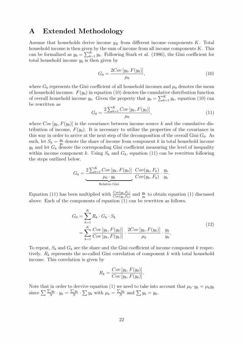
A Extended Methodology
Assume that households derive income yK from different income components K. Totalhousehold income is then given by the sum of income from all income components K. Thiscan be formalized as y0 =
∑Kk=1 yk. Following Stark et al. (1986), the Gini coefficient for
total household income y0 is then given by
G0 =2Cov [y0, F (y0)]
µ0
, (10)
where G0 represents the Gini coefficient of all household incomes and µ0 denotes the meanof household incomes. F (y0) in equation (10) denotes the cumulative distribution functionof overall household income y0. Given the property that y0 =
∑Kk=1 yk, equation (10) can
be rewritten as
G0 =2∑K
k=1Cov [yk, F (y0)]
µ0
, (11)
where Cov [yk, F (y0)] is the covariance between income source k and the cumulative dis-tribution of income, F (y0). It is necessary to utilize the properties of the covariance inthis way in order to arrive at the next step of the decomposition of the overall Gini G0. Assuch, let Sk = yk
y0denote the share of income from component k in total household income
y0 and let Gk denote the corresponding Gini coefficient measuring the level of inequalitywithin income component k. Using Sk and Gk, equation (11) can be rewritten followingthe steps outlined below.
G0 =2∑K
k=1Cov [yk, F (y0)]
µ0 · y0︸ ︷︷ ︸Relative Gini
·Cov(yk, Fk)
Cov(yk, Fk)· ykyk.
Equation (11) has been multiplied with Cov(yk,Fk)Cov(yk,Fk)
and ykyk
to obtain equation (1) discussed
above. Each of the components of equation (1) can be rewritten as follows.
G0 =K∑k=1
Rk ·Gk · Sk
=K∑k=1
Cov [yk, F (y0)]
Cov [yk, F (yk)]· 2Cov [yk, F (yk)]
µk
· yky0,
(12)
To repeat, Sk and Gk are the share and the Gini coefficient of income component k respec-tively. Rk represents the so-called Gini correlation of component k with total householdincome. This correlation is given by
Rk =Cov [yk, F (y0)]
Cov [yk, F (yk)].
Note that in order to dervive equation (1) we need to take into account that µ0 ·yk = µky0since
∑ ∑yk
N· yk =
∑yk
N·∑yk with µk =
∑yk
Nand
∑yk = y0.
22
B Additional Figures and Tables
Figure 1: Box 2 in Azevedo et al. (2013)
Table 8: Dynamic Decomposition - 1993 to 2014
Effect Gini %-ChangeLabour Income 0.007 1.0%Government Grants -0.072 -10.6%Remittances 0.005 0.7%Investment -0.01 -1.5%
Note: Own Calculations using PSLSD and NIDSweightedNumber of paths = 40320
Number of factors = 8
23
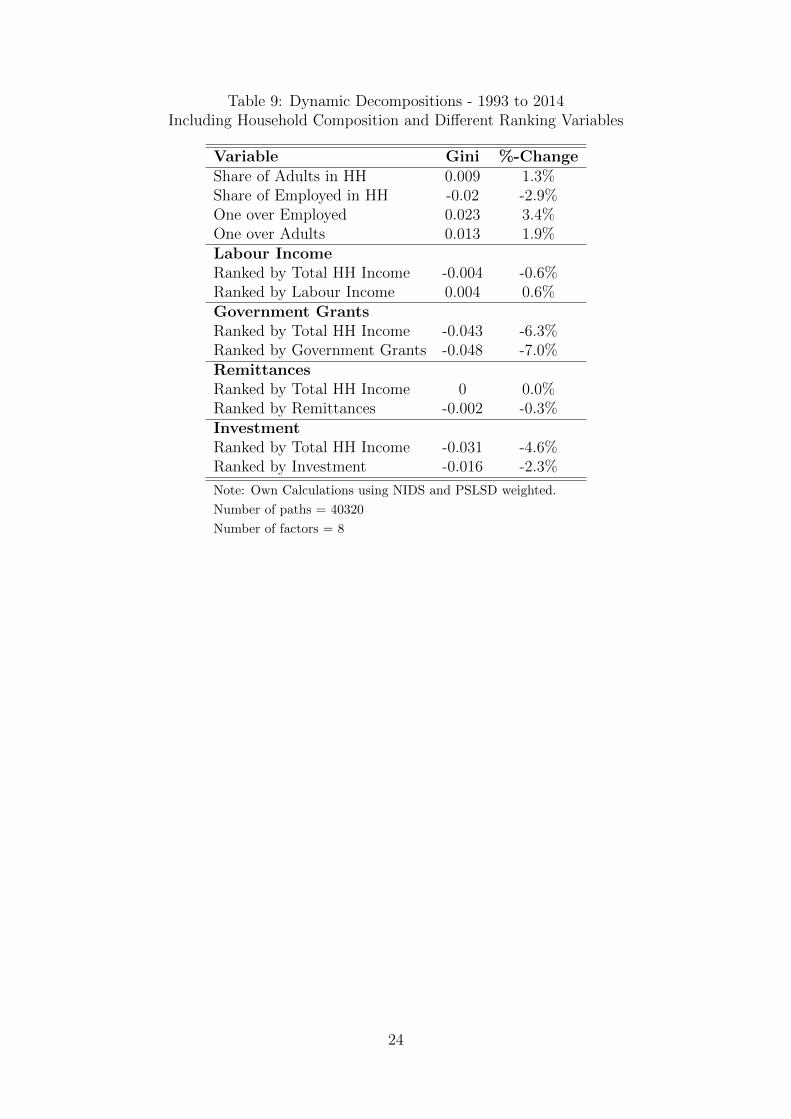
Table 9: Dynamic Decompositions - 1993 to 2014Including Household Composition and Different Ranking Variables
Variable Gini %-ChangeShare of Adults in HH 0.009 1.3%Share of Employed in HH -0.02 -2.9%One over Employed 0.023 3.4%One over Adults 0.013 1.9%Labour IncomeRanked by Total HH Income -0.004 -0.6%Ranked by Labour Income 0.004 0.6%Government GrantsRanked by Total HH Income -0.043 -6.3%Ranked by Government Grants -0.048 -7.0%RemittancesRanked by Total HH Income 0 0.0%Ranked by Remittances -0.002 -0.3%InvestmentRanked by Total HH Income -0.031 -4.6%Ranked by Investment -0.016 -2.3%
Note: Own Calculations using NIDS and PSLSD weighted.
Number of paths = 40320
Number of factors = 8
24
References
[1] Azevedo, J., Inchaust, G., and Sanfelice, V. Decomposing the recent in-equality decline in latin america,. Tech. rep., The World Bank, 2013.
[2] Barros, R. P. D., Carvalho, M. D., Franco, S., and Mendonca, R. Umaanalise das principais causas da queda recente na desigualdade de renda brasileira.Tech. Rep. 1203, Instituto de Pesquisa Economica Aplicada (Ipea), August 2006.
[3] Leibbrandt, M., Finn, A., and Woolard, I. Describing and decomposing post-apartheid income inequality in south africa. Development Southern Africa (2012).
[4] Leibbrandt, M., Woolard, I., Finn, A., and Argent, J. Trends in southafrican income distribution and poverty since the fall of apartheid. OECD Social,Employment and Migration Working Papers, 101 (2010).
[5] Lerman, R. I., and Yitzhaki, S. Income inequality effects by income source: anew approach and applications to the united states. The Review of Economics andStatistics (1985), 151–156.
[6] NIDS. Wave 3 overview. Tech. rep., National Planning Comission, 2013.
[7] SALDRU. South Africans rich and poor: baseline household statistics. Project forStatistics on Living Standards. Southern African Labour and Development ResearchUnit, School of Economics, University of Cape Town, 1994.
[8] Schiel, R., Leibbrandt, M., and Lam, D. Assessing the impact of social grantson inequality: A South African case study. Contemporary Issues in DevelopmentEconomics. Palgrave MacMillan, New York, 2016, ch. 8, pp. 112 – 135.
[9] Shorrocks, A. F. Inequality decomposition by factor components. Econometrica:Journal of the Econometric Society (1982), 193–211.
[10] Stark, O., Taylor, J. E., and Yitzhaki, S. Remittances and inequality. TheEconomic Journal 96, 383 (1986), 722–740.
Data Sources
[1] SALDRU. Project for Statistics on Living Standards and Development - PSLSD[dataset]. Southern Africa Labour and Development Research Unit [producer], CapeTown (2012). Version 2.0.
[2] SALDRU. National Income Dynamics Study 2008, Wave 1 [dataset]. Southern AfricaLabour and Development Research Unit [producer], Cape Town (2015). Version 6.0.
[3] SALDRU. National Income Dynamics Study 2014-2015, Wave 4 [dataset]. South-ern Africa Labour and Development Research Unit [producer], Cape Town (2015).Version 1.0.
25

The Southern Africa Labour and Development Research Unit (SALDRU) conducts research directed at improving the well-being of South Africa’s poor. It was established in 1975. Over the next two decades the unit’s research played a central role in documenting the human costs of apartheid. Key projects from this period included the Farm Labour Conference (1976), the Economics of Health Care Conference (1978), and the Second Carnegie Enquiry into Poverty and Development in South Africa (1983-86). At the urging of the African National Congress, from 1992-1994 SALDRU and the World Bank coordinated the Project for Statistics on Living Standards and Development (PSLSD). This project provide baseline data for the implementation of post-apartheid socio-economic policies through South Africa’s fi rst non-racial national sample survey. In the post-apartheid period, SALDRU has continued to gather data and conduct research directed at informing and assessing anti-poverty policy. In line with its historical contribution, SALDRU’s researchers continue to conduct research detailing changing patterns of well-being in South Africa and assessing the impact of government policy on the poor. Current research work falls into the following research themes: post-apartheid poverty; employment and migration dynamics; family support structures in an era of rapid social change; public works and public infrastructure programmes, fi nancial strategies of the poor; common property resources and the poor. Key survey projects include the Langeberg Integrated Family Survey (1999), the Khayelitsha/Mitchell’s Plain Survey (2000), the ongoing Cape Area Panel Study (2001-) and the Financial Diaries Project.
www.saldru.uct.ac.za
Level 3, School of Economics Building, Middle Campus, University of Cape Town
Private Bag, Rondebosch 7701, Cape Town, South Africa
Tel: +27 (0)21 650 5696
Fax: +27 (0) 21 650 5797
Web: www.saldru.uct.ac.za
southern africa labour and development research unit


![WHAT DRIVES YOUTH UNEMPLOYMENT AND WHAT … · (J-PAL); Vimal Ranchhod, Cecil Mlatsheni and Callie Ardington (Southern Africa Labour and Development Research Unit [SALDRU], UCT);](https://img.pdfslide.net/doc/110x75/5f0c97297e708231d4362947/what-drives-youth-unemployment-and-what-j-pal-vimal-ranchhod-cecil-mlatsheni.jpg)