Embed Size (px)
Citation preview
Space-Time
Discontinuous Galerkin Methods
for Convection-Diffusion Problems
Application to Wet-Chemical Etching
The research described in this thesis was undertaken at the Group of Numerical
Analysis and Computational Mechanics, Department of Applied Mathematics, Fac-
ulty EWI, Universiteit Twente, Enschede.
The funding of the research was provided by the Dutch Technology Foundation STW
through research project TWI. 5453 (Analysis and control of transport phenomena
in wet-chemical etching processes).
c© J.J. Sudirham, Enschede, 2005
No part of this work may be reproduced by print, photocopy or any other means without the
permission in writing from the author.
Printed by Wohrmann Printing Service, Zutphen, The Netherlands
The summary in Dutch was done by Ruud van Damme
ISBN 90-365-2287-0
SPACE-TIME DISCONTINUOUS GALERKIN METHODS
FOR CONVECTION-DIFFUSION PROBLEMS
APPLICATION TO WET-CHEMICAL ETCHING
DISSERTATION
to obtain
the doctor’s degree at the University of Twente,
on the authority of the rector magnificus,
prof. dr. W.H.M. Zijm,
on account of the decision of the graduation committee,
to be publicly defended
on Thursday 8 December 2005 at 15.00
by
Janivita Joto Sudirham
born on 24 May 1974
in Jakarta, Indonesia
This dissertation has been approved by the promoter
Prof. dr. ir. J.J.W. van der Vegt
and the assistant promoter
dr. R.M.J. van Damme
Praise be to Allah, who hath guided us to this work:
never could we have found guidance,
had it not been for the guidance of Allah. (Q.S. 7:43)
with the power and skill did We construct the firmament,
for it is We who create the vastness of space. (Q.S. 51:47)
this thesis is dedicated
to my mother and my father
to my husband

Summary
Etching is an important step in the fabrication of microstructures, during which a
pattern is transferred onto the background material by etching away part of the
material. In industrial applications, an acid fluid is used to dissolve the material and
it is therefore called wet-chemical etching. The transport of the acid fluid and etching
products during wet-chemical etching is important to obtain the desired patterns.
However, it is generally complicated to control the process. Numerical simulations
are then used to study transport phenomena during etching. Due to the complexity
of the phenomena and the geometry of the structures, wet-chemical etching processes
require numerical techniques which can deal with deforming elements to accommodate
the movement of the etching cavity boundary.
In this thesis we discuss space-time discontinuous Galerkin (DG) finite element
methods for transport phenomena in incompressible flows. The methods, which simul-
taneously discretize the equations in space and time, provide the necessary flexibility
to deal with time deforming meshes and mesh adaptation. In particular, we discuss
space-time DG methods for the advection-diffusion equation, which governs the con-
centration of the acid fluid, and for the incompressible Navier-Stokes equations to
model the flow of the acid fluid inside and outside the etching cavity. We provide a
detailed theoretical analysis of the stability of the newly developed methods, as well
as some simple numerical tests to investigate the accuracy of the methods.
We demonstrate the capabilities of the newly developed methods to wet-chemical
etching processes. Two cases of diffusion-controlled etching are discussed: etching of
a slit, which can be considered as a two dimensional problem, and etching of a circular
hole. The latter we solve without using the fact that the problem has a rotational
symmetry, this we have done in order to show that a fully three dimensional simulation
is indeed possible. For simple cases, the numerical results show good agreement
with the predictions obtained with an analytical approach. Moreover, the numerical
simulations can give a complete description of the time evolution of the shape of
the etching cavity. The numerical simulations of convection-dominated etching of a
slit coupled with the Stokes equations give a detailed description of the transport
phenomena in wet-chemical etching inside the cavity.
vii

Samenvatting
Het etsproces is een essentieel onderdeel in het fabricatieproces van microstructuren.
Er wordt in dit proces als het ware een zeker patroon, dat vastgelegd is in het zoge-
naamde masker, gecopieerd op het materiaal door dit materiaal weg te etsen op de
plaatsen waar het masker het materiaal niet beschermt. In industriele toepassingen
wordt een zure vloeistof gebruikt om het materiaal op te lossen, en deze manier van
etsen wordt daarom nat-chemisch etsen genoemd. Het transport van de zure vloeistof
en het ets-materiaal bepaalt in hoge mate het uiteindelijke patroon. Het is echter
zo, dat dit proces moeilijk te beheersen is. Daarom worden numerieke simluaties
gebruikt om de transportfenomenen beter te begrijpen. Door de complexiteit van
alle fenomenen alsook de geometrie van de structuren, is het noodzakelijk dat deze
numerieke simulaties kunnen omgaan met deformerende elementen om de beweging
van het scheidingsoppervlak tussen daar waar wel en waar niet ge-etst is, nauwkeurig
te kunnen volgen.
In dit proefschrift bediscussieren we Galerkin methoden waarvan de basisfuncties
zowel in de ruimtelijke richting als in de tijdrichting discontinu mogen zijn (DG).
Doel is om met deze methoden transportproblemen van incompressibele vloeistoffen
te beschrijven. Deze methoden, die tegelijkertijd de vergelijkingen in de ruimte en
in tijd discretizeren, staan garant voor de noodzakelijke flexibiliteit die nodig is om
bewegende roosters en ook topologisch veranderende roosters, aan te kunnen. In
het bijzonder bespreken we DG methoden, in plaats en in tijd, voor de advectie-
diffusievergelijking – deze bepaalt de concentratie van de zure vloeistof – en voor
de Navier-Stokesvergelijkingen. Deze laatste zijn nodig om de beweging van de zure
vloeistof in het hele domein nauwkeurig te beschrijven. We geven in dit proefschrift
ook een gedetailleerde theoretische analyse van de stabiliteit van de ontworpen nu-
merieke methoden. Voorts voeren we enkele eenvoudige numerieke tests uit om de
nauwkeurigheid van de methoden te onderzoeken en de methoden te valideren.
We demonstreren de mogelijkheden van deze nieuwe methoden aan de hand van
nat-chemisch etsprocessen. Twee gevallen van etsen, waarbij diffusie het etsproces
domineeert, worden besproken. Op de eerste plaats een etsprobleem waarbij het
masker een (zeer lange) spleet heeft, die overal even breed is. Dit geval kunnen we
effectief beschouwen als een tweedimensionaal probleem in de ruimte. Op de tweede
ix
plaats bekijken we het proces waarbij het masker precies een cirkelvormig gaatje
bevat. Dit probleem hebben we door kunnen rekenen zonder gebruik te maken van de
cirkelsymmetrie die het probleem in zich heeft – dit hebben we gedaan om aan te tonen
dat berekeningen in drie ruimtedimensies inderdaad tot de mogelijkheden behoren.
De numerieke resultaten laten in alle gevallen een zeer goede overeenkomst zien met
de analytische voorspellingen. Sterker nog, de numerieke simulaties geven een be-
schrijving van de verandering van de etsholte als functie van de tijd. De numerieke
simulaties van de vergelijkingen waarin de vloeistofbeweging wordt beschreven door
de zogenaamde vergelijkingen van Stokes, zijn ook uitgevoerd voor het nat-chemisch
etsen met een masker met een zeer lange spleet en geven een nauwkeurige beschrijving
van de transportverschijnselen in de etsholte.
x
Contents
Summary vii
Samenvatting ix
Contents xi
1 Introduction 1
1.1 The etching process . . . . . . . . . . . . . . . . . . . . . . . . . . . . 1
1.2 Overview of mathematical models for wet-chemical etching . . . . . . 5
1.3 Approach . . . . . . . . . . . . . . . . . . . . . . . . . . . . . . . . . . 7
1.4 Objectives . . . . . . . . . . . . . . . . . . . . . . . . . . . . . . . . . . 8
1.5 Outline of the thesis . . . . . . . . . . . . . . . . . . . . . . . . . . . . 8
2 Mathematical Modeling of Wet-Chemical Etching Processes 11
2.1 Introduction . . . . . . . . . . . . . . . . . . . . . . . . . . . . . . . . . 11
2.2 Governing equations for wet-chemical etching processes . . . . . . . . 12
2.3 Dimensionless form of the governing equations . . . . . . . . . . . . . 14
3 Discontinuous Galerkin Methods for Elliptic Equations 17
3.1 Introduction . . . . . . . . . . . . . . . . . . . . . . . . . . . . . . . . . 17
3.2 Model problem . . . . . . . . . . . . . . . . . . . . . . . . . . . . . . . 18
3.3 Finite element spaces and trace operators . . . . . . . . . . . . . . . . 19
3.4 DG weak formulations . . . . . . . . . . . . . . . . . . . . . . . . . . . 21
3.5 Adaptation . . . . . . . . . . . . . . . . . . . . . . . . . . . . . . . . . 25
3.5.1 Adaptation algorithms . . . . . . . . . . . . . . . . . . . . . . . 26
3.5.2 The efficiency of the method . . . . . . . . . . . . . . . . . . . 28
3.6 Concluding remarks . . . . . . . . . . . . . . . . . . . . . . . . . . . . 31
4 A Space-Time Discontinuous Galerkin Method for the Advection-
Diffusion Equation in Time-Dependent Domains 33
4.1 Introduction . . . . . . . . . . . . . . . . . . . . . . . . . . . . . . . . . 33
4.2 The advection-diffusion equation . . . . . . . . . . . . . . . . . . . . . 34
xi
4.3 Space-time description, finite element spaces and trace operators . . . 35
4.3.1 Definition of space-time slabs, elements and faces . . . . . . . . 35
4.3.2 Finite element spaces and trace operators . . . . . . . . . . . . 36
4.3.3 Lifting operators . . . . . . . . . . . . . . . . . . . . . . . . . . 39
4.4 Space-time DG discretization for the advection-diffusion . . . . . . . . 39
4.4.1 Weak formulation for the auxiliary variable . . . . . . . . . . . 40
4.4.2 Weak formulation for the primal variable . . . . . . . . . . . . 41
4.5 Consistency, coercivity, and stability . . . . . . . . . . . . . . . . . . . 46
4.5.1 Main results . . . . . . . . . . . . . . . . . . . . . . . . . . . . . 46
4.5.2 Detailed proofs . . . . . . . . . . . . . . . . . . . . . . . . . . . 48
4.6 Error estimates and hp-convergence . . . . . . . . . . . . . . . . . . . . 51
4.6.1 Bounds for the interpolation error . . . . . . . . . . . . . . . . 51
4.6.2 Global estimates . . . . . . . . . . . . . . . . . . . . . . . . . . 54
4.6.3 Error estimates at specific time levels . . . . . . . . . . . . . . 55
4.6.4 Proofs . . . . . . . . . . . . . . . . . . . . . . . . . . . . . . . . 58
4.7 Numerical results . . . . . . . . . . . . . . . . . . . . . . . . . . . . . . 60
4.8 Concluding remarks . . . . . . . . . . . . . . . . . . . . . . . . . . . . 66
5 A Space-Time Discontinuous Galerkin Method for Incompressible
Flows 69
5.1 Introduction . . . . . . . . . . . . . . . . . . . . . . . . . . . . . . . . . 69
5.2 The incompressible flows . . . . . . . . . . . . . . . . . . . . . . . . . . 70
5.3 Space-time elements, finite element spaces and trace operators . . . . 72
5.3.1 Definition of space-time slabs, elements and faces . . . . . . . . 72
5.3.2 Finite element spaces and trace operators . . . . . . . . . . . . 72
5.3.3 Lifting operators . . . . . . . . . . . . . . . . . . . . . . . . . . 74
5.4 Space-time DG discretization for the Oseen equations . . . . . . . . . 74
5.4.1 Weak formulation for the auxiliary variable . . . . . . . . . . . 75
5.4.2 Weak formulation for the primal variables . . . . . . . . . . . . 76
5.4.3 Weak formulation for the continuity equation . . . . . . . . . . 81
5.5 Stability analysis . . . . . . . . . . . . . . . . . . . . . . . . . . . . . . 82
5.6 Numerical results . . . . . . . . . . . . . . . . . . . . . . . . . . . . . . 90
5.7 Concluding remarks . . . . . . . . . . . . . . . . . . . . . . . . . . . . 93
6 Simulation of Wet-Chemical Etching Processes 95
6.1 Introduction . . . . . . . . . . . . . . . . . . . . . . . . . . . . . . . . . 95
6.2 Discretization of the equation for the moving boundary . . . . . . . . 95
6.3 Construction of an initial computational mesh . . . . . . . . . . . . . . 96
6.4 Diffusion-controlled wet-chemical etching . . . . . . . . . . . . . . . . . 97
6.4.1 Algorithm for the simulations . . . . . . . . . . . . . . . . . . . 97
6.4.2 Diffusion-controlled etching of a slit . . . . . . . . . . . . . . . 99
6.4.3 Diffusion-controlled etching of a circular hole . . . . . . . . . . 103
xii
6.5 Convection-dominated wet-chemical etching . . . . . . . . . . . . . . . 109
6.5.1 Convection-dominated etching with a prescribed velocity field . 109
6.5.2 Fully coupled convection-dominated etching using the Stokes
equations . . . . . . . . . . . . . . . . . . . . . . . . . . . . . . 112
7 Conclusions and Future Research 117
7.1 Conclusions . . . . . . . . . . . . . . . . . . . . . . . . . . . . . . . . . 117
7.2 Recommendations for future research . . . . . . . . . . . . . . . . . . . 118
A Algebraic System for the Space-Time Discontinuous Galerkin Dis-
cretizations 119
A.1 Algebraic system for the advection-diffusion equation . . . . . . . . . . 119
A.1.1 Algebraic system for the diffusive part . . . . . . . . . . . . . . 119
A.1.2 Algebraic system for the advective part . . . . . . . . . . . . . 123
A.2 Algebraic system for incompressible flows . . . . . . . . . . . . . . . . 124
A.2.1 Algebraic system for the diffusive and convective parts . . . . . 125
A.2.2 Algebraic system for the pressure term and incompressibility
constraint . . . . . . . . . . . . . . . . . . . . . . . . . . . . . . 126
A.2.3 Algebraic system for the stability term . . . . . . . . . . . . . . 128
B Anisotropic Interpolation Error Estimates 131
B.1 Preliminaries . . . . . . . . . . . . . . . . . . . . . . . . . . . . . . . . 131
B.2 Interpolation error estimates on the reference element . . . . . . . . . 134
B.3 Interpolation error estimates on the space-time element . . . . . . . . 137
Bibliography 143
Acknowledgements 149
Ringkasan 151
xiii

Chapter 1
Introduction
1.1 The etching process
Nowadays, many devices are assembled from large numbers of small but important
components. These components contain extremely small features and are produced
with special fabrication techniques. One of these techniques is photolithography in
which a pattern with small features is transferred onto a photosensitive substrate and
the background material is chemically etched away to produce the desired pattern.
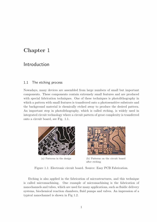
An important step in photolithography, which is called etching, is widely used in
integrated circuit technology where a circuit pattern of great complexity is transferred
onto a circuit board, see Fig. 1.1.
(a) Patterns in the design (b) Patterns on the circuit board
after etching
Figure 1.1: Electronic circuit board. Source: Easy PCB Fabrication.
Etching is also applied in the fabrication of microstructures, and this technique
is called micromachining. One example of micromachining is the fabrication of
nanochannels and tubes, which are used for many applications, such as fluidic delivery
systems, biochemical reaction chambers, fluid pumps and valves. An impression of a
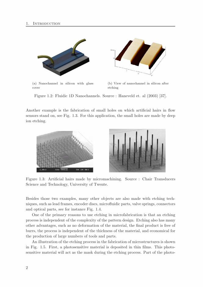
typical nanochannel is shown in Fig 1.2.
1
1. Introduction
(a) Nanochannel in silicon with glass
cover
(b) View of nanochannel in silicon after
etching
Figure 1.2: Fluidic 1D Nanochannels. Source : Haneveld et. al (2003) [37].
Another example is the fabrication of small holes on which artificial hairs in flow
sensors stand on, see Fig. 1.3. For this application, the small holes are made by deep
ion etching.
Figure 1.3: Artificial hairs made by micromachining. Source : Chair Transducers
Science and Technology, University of Twente.
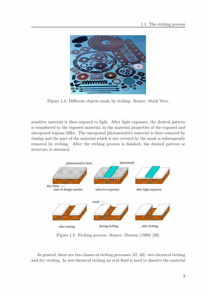
Besides those two examples, many other objects are also made with etching tech-
niques, such as lead frames, encoder discs, microfluidic parts, valve springs, connectors
and optical parts, see for instance Fig. 1.4.
One of the primary reasons to use etching in microfabrication is that an etching
process is independent of the complexity of the pattern design. Etching also has many
other advantages, such as no deformation of the material, the final product is free of
burrs, the process is independent of the thickness of the material, and economical for
the production of large numbers of tools and parts.
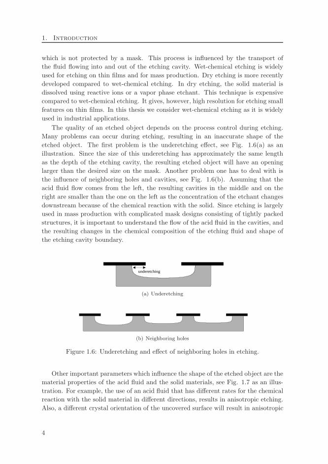
An illustration of the etching process in the fabrication of microstructures is shown
in Fig. 1.5. First, a photosensitive material is deposited in thin films. This photo-
sensitive material will act as the mask during the etching process. Part of the photo-
2
1.1. The etching process
Figure 1.4: Different objects made by etching. Source: Stork Veco.
sensitive material is then exposed to light. After light exposure, the desired pattern
is transferred to the exposed material, as the material properties of the exposed and
unexposed regions differ. The unexposed photosensitive material is then removed by
rinsing and the part of the material which is not covered by the mask is subsequently
removed by etching. After the etching process is finished, the desired pattern or
structure is obtained.
mask
photomaskphotosensitive layer
after light exposure
after rinsing during etching after etching
thin filmsselective exposurestart of design transfer
Figure 1.5: Etching process. Source: Driesen (1999) [29].
In general, there are two classes of etching processes [47, 48]: wet-chemical etching
and dry etching. In wet-chemical etching an acid fluid is used to dissolve the material
3
1. Introduction
which is not protected by a mask. This process is influenced by the transport of
the fluid flowing into and out of the etching cavity. Wet-chemical etching is widely
used for etching on thin films and for mass production. Dry etching is more recently
developed compared to wet-chemical etching. In dry etching, the solid material is
dissolved using reactive ions or a vapor phase etchant. This technique is expensive
compared to wet-chemical etching. It gives, however, high resolution for etching small
features on thin films. In this thesis we consider wet-chemical etching as it is widely
used in industrial applications.
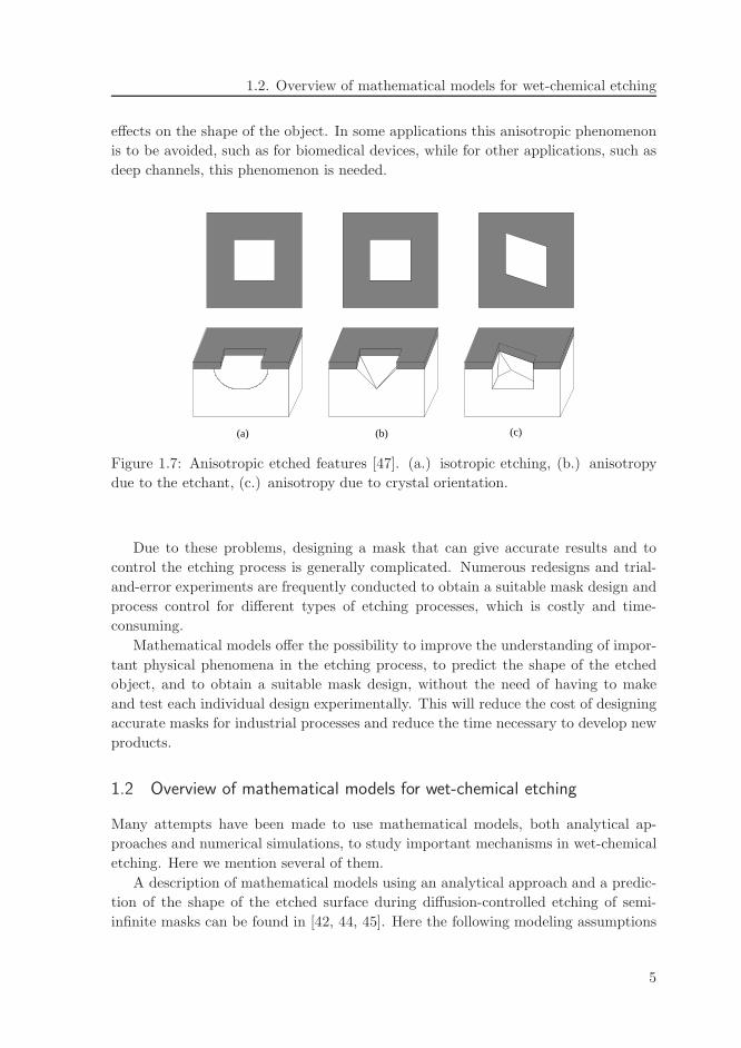
The quality of an etched object depends on the process control during etching.
Many problems can occur during etching, resulting in an inaccurate shape of the
etched object. The first problem is the underetching effect, see Fig. 1.6(a) as an
illustration. Since the size of this underetching has approximately the same length
as the depth of the etching cavity, the resulting etched object will have an opening
larger than the desired size on the mask. Another problem one has to deal with is
the influence of neighboring holes and cavities, see Fig. 1.6(b). Assuming that the
acid fluid flow comes from the left, the resulting cavities in the middle and on the
right are smaller than the one on the left as the concentration of the etchant changes
downstream because of the chemical reaction with the solid. Since etching is largely
used in mass production with complicated mask designs consisting of tightly packed
structures, it is important to understand the flow of the acid fluid in the cavities, and
the resulting changes in the chemical composition of the etching fluid and shape of
the etching cavity boundary.
underetching
(a) Underetching
(b) Neighboring holes
Figure 1.6: Underetching and effect of neighboring holes in etching.
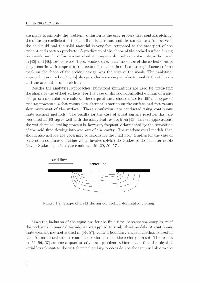
Other important parameters which influence the shape of the etched object are the
material properties of the acid fluid and the solid materials, see Fig. 1.7 as an illus-
tration. For example, the use of an acid fluid that has different rates for the chemical
reaction with the solid material in different directions, results in anisotropic etching.
Also, a different crystal orientation of the uncovered surface will result in anisotropic
4
1.2. Overview of mathematical models for wet-chemical etching
effects on the shape of the object. In some applications this anisotropic phenomenon
is to be avoided, such as for biomedical devices, while for other applications, such as
deep channels, this phenomenon is needed.
(a) (b) (c)
Figure 1.7: Anisotropic etched features [47]. (a.) isotropic etching, (b.) anisotropy
due to the etchant, (c.) anisotropy due to crystal orientation.
Due to these problems, designing a mask that can give accurate results and to
control the etching process is generally complicated. Numerous redesigns and trial-
and-error experiments are frequently conducted to obtain a suitable mask design and
process control for different types of etching processes, which is costly and time-
consuming.
Mathematical models offer the possibility to improve the understanding of impor-
tant physical phenomena in the etching process, to predict the shape of the etched
object, and to obtain a suitable mask design, without the need of having to make
and test each individual design experimentally. This will reduce the cost of designing
accurate masks for industrial processes and reduce the time necessary to develop new
products.
1.2 Overview of mathematical models for wet-chemical etching
Many attempts have been made to use mathematical models, both analytical ap-
proaches and numerical simulations, to study important mechanisms in wet-chemical
etching. Here we mention several of them.
A description of mathematical models using an analytical approach and a predic-
tion of the shape of the etched surface during diffusion-controlled etching of semi-
infinite masks can be found in [42, 44, 45]. Here the following modeling assumptions
5
1. Introduction
are made to simplify the problem: diffusion is the only process that controls etching,
the diffusion coefficient of the acid fluid is constant, and the surface reaction between
the acid fluid and the solid material is very fast compared to the transport of the
etchant and reaction products. A prediction of the shape of the etched surface during
time evolution for diffusion-controlled etching of a slit and a circular hole, is discussed
in [43] and [46], respectively. These studies show that the shape of the etched objects
is symmetric with respect to the center line, and there is a strong influence of the
mask on the shape of the etching cavity near the edge of the mask. The analytical
approach presented in [43, 46] also provides some simple rules to predict the etch rate
and the amount of underetching.
Besides the analytical approaches, numerical simulations are used for predicting
the shape of the etched surface. For the case of diffusion-controlled etching of a slit,
[66] presents simulation results on the shape of the etched surface for different types of
etching processes: a fast versus slow chemical reaction on the surface and fast versus
slow movement of the surface. These simulations are conducted using continuous
finite element methods. The results for the case of a fast surface reaction that are
presented in [66] agree well with the analytical results from [43]. In real applications,
the wet-chemical etching process is, however, frequently dominated by the convection
of the acid fluid flowing into and out of the cavity. The mathematical models then
should also include the governing equations for the fluid flow. Studies for the case of
convection-dominated etching which involve solving the Stokes or the incompressible
Navier-Stokes equations are conducted in [29, 56, 57].
acid flowcenter line
Figure 1.8: Shape of a slit during convection-dominated etching.
Since the inclusion of the equations for the fluid flow increases the complexity of
the problems, numerical techniques are applied to study these models. A continuous
finite element method is used in [56, 57], while a boundary element method is used in
[29]. All numerical studies conducted so far consider the etching of a slit. The results
in [29, 56, 57] assume a quasi steady-state problem, which means that the physical
variables relevant to the wet-chemical etching process do not change much due to the
6
1.3. Approach
change of the position of the etched surface.
Convection also influences the shape of the cavity which is no longer symmetric
with respect to the center line of the slit since the concentration of the etchant in
the cavity is influenced by the convection. A sketch of the shape of a slit during
convection-dominated etching is given in Fig. 1.8.
1.3 Approach
Mathematical models offer the possibility to study the physical phenomena during
etching and to predict the shape of an etched object. For relatively simple models
analytical techniques can be used to predict the final shape of an etched object, but
when the transport phenomena in the wet-chemical etching processes or the shape of
the object become more complex, then numerical simulations are more useful since
they require less modeling assumptions.
The numerical simulation of wet-chemical etching is, however, a non-trivial task.
The numerical method should be able to compute the fluid flow and transport phe-
nomena in complex and time-dependent geometries. The numerical technique should
also be able to adapt the computational mesh locally in order to capture small struc-
tures, such as boundary layers and singularities accurately and efficiently. One of the
techniques that has these features is the discontinuous Galerkin (DG) finite element
method.
The DG method is a class of finite element methods that uses basis functions that
are discontinuous across the element boundary. This has several important benefits,
in particular, DG methods can achieve higher order accuracy on unstructured meshes,
are suitable for local adaptation, and efficient on parallel computers. These features
make DG methods an excellent numerical technique for the simulation of wet-chemical
etching.
An important aspect in the simulation of wet-chemical etching is that we need to
perform computations on time-dependent flow domains where the shape of the domain
is part of the solution. This requires the use of moving and deforming elements which
is greatly facilitated by the use of a space-time discretization.
In a space-time discretization, there is no separation between the space and time
variables. This discretization technique is beneficial for problems defined on time-
dependent domains, such as occur in fluid-solid interaction problems and other prob-
lems with moving interfaces. The space-time DG method is proposed in [41], together
with a theoretical analysis of this technique for multidimensional scalar conservation
laws (see also [15]). In [64, 65], the space-time DG method is extended to non-
linear hyperbolic systems in particular the Euler equations of gas dynamics. The
space-time DG method provides optimal efficiency to adapt and deform the mesh to
accommodate for the changes in the domain boundaries, while maintaining a conser-
vative numerical discretization. Since simulations of wet-chemical etching processes
7
1. Introduction
require a numerical technique that can deal with the movement of the etching cavity
boundary, space-time DG methods are well suited for the simulation of wet-chemical
etching. In this thesis we consider the development and analysis of space-time DG
methods for the advection-diffusion equation and the incompressible (Navier)-Stokes
equations and we apply these techniques to the simulation of wet-chemical etching.
1.4 Objectives
The research documented in this thesis has two main objectives: the development
of a space-time discontinuous Galerkin finite element method for the simulation of
transport phenomena in incompressible flow and the application and demonstration
of this technique to wet-chemical etching of different objects.
The first objective requires the development of a space-time DG method suitable
for solving: (a) the advection-diffusion equation for an active etching component
in a time-dependent domain and (b) the incompressible (Navier)-Stokes equations
which control the fluid flow inside and outside the etching cavity. Also, a detailed
theoretical analysis is necessary to investigate the accuracy, stability, and convergence
of the numerical methods, which is essential to obtain a robust and accurate numerical
technique.
The second objective focusses on the simulation of wet-chemical etching processes.
The capability of the newly developed method to simulate different types of etching
processes will be investigated using a sequence of increasingly more complicated model
problems. First, simulations of diffusion-controlled etching will be conducted to study
the potential of the space-time DG method for this type of etching. These simulations
are also used to investigate the accuracy of the computed shape of the moving bound-
ary by comparing them with analytical approximations and other numerical results.
Next, simulations of convection-dominated etching are conducted to study the trans-
port phenomena in wet-chemical etching in a more realistic model by including the
velocity field of the acid fluid into the model. This is intended to study the influence
of the convection of the acid fluid on the shape of the cavity.
1.5 Outline of the thesis
The outline of this thesis is as follows.
In Chapter 2 the governing equations relevant for wet-chemical etching processes
are presented. First, the equations are formulated in their usual form. Next, we
introduce reference values for wet-chemical etching processes and use these values to
write the equations in dimensionless form.
The next three chapters will be devoted to the development and analysis of DG
methods suitable for the simulation of wet-chemical etching. First, the discretization
of elliptic partial differential equations with DG methods is discussed in Chapter
8
1.5. Outline of the thesis
3, which serves as an introduction to DG discretizations for second-order partial
differential equations. We also present some simple one dimensional numerical tests
to demonstrate the accuracy of the DG methods, in particular their suitability for
hp-adaptation.
In Chapter 4, we discuss the space-time DG discretization for the convection-
diffusion equation in time-dependent flow domains and give a complete derivation
of this numerical method. A detailed theoretical analysis of the stability and error
estimates is also given. This chapter is completed with some simple numerical tests to
verify the theoretical analysis of the convergence rate of the space-time DG method.
The space-time DG discretization for time-dependent incompressible flows is dis-
cussed in Chapter 5. Special attention is given to the extension of the DG techniques
developed for steady-state problems to problems on time-dependent domains. The
theoretical analysis of the stability of the method is given, as well as some simple
tests to investigate the accuracy of the method.
Simulation results for different types of wet-chemical etching processes are pre-
sented in Chapter 6. First, we describe the DG discretization for an equation govern-
ing the movement of the etching surface together with the construction of an initial
space-time mesh for the computations.
For the etching simulations we consider both diffusion and convection-dominated
etching. For diffusion-controlled etching, two cases are discussed: the etching of a slit,
which can be seen as a two dimensional problem, and the etching of a circular hole,
as an example of a three dimensional problem. For convection-dominated etching, we
consider the etching of a slit. First, we only consider the case when the velocity field of
the etchant concentration throughout the computational domain is given. Next, the
computations of the transport of the etchant are fully coupled with the computation
of the velocity field using the time-dependent Stokes equations.
Finally, conclusions and recommendations for future research are presented in
Chapter 7.
9

Chapter 2
Mathematical Modeling of Wet-Chemical Etching
Processes
2.1 Introduction
In this chapter we discuss the main transport phenomena involved in wet-chemical
etching processes and describe the governing equations.
x
x
Γ
Γ
Γ
2
1
mask mask
solid materialcavity surface Γ ( t )
Γ ( t = 0 )
Ω ( t )
fluid flow
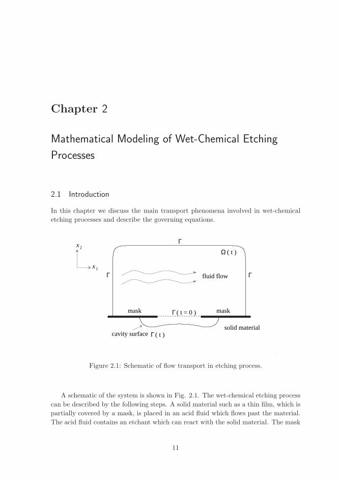
Figure 2.1: Schematic of flow transport in etching process.
A schematic of the system is shown in Fig. 2.1. The wet-chemical etching process
can be described by the following steps. A solid material such as a thin film, which is
partially covered by a mask, is placed in an acid fluid which flows past the material.
The acid fluid contains an etchant which can react with the solid material. The mask
11
2. Mathematical Model of Wet-Chemical Etching
is made of a different material that does not react with the acid. The etchant is
transported by convection and diffusion to the uncovered part of the solid material
where it reacts, thereby dissolving the unprotected part of the material, and develops a
small cavity. As etching proceeds, the shape of the cavity evolves with time according
to the etch rate distribution along the cavity, which depends on the concentration of
the etchant inside the flow domain. In the next sections, we discuss in more detail
the governing equations which describe wet-chemical etching processes.
2.2 Governing equations for wet-chemical etching processes
In this section we discuss the governing equations for each subproblem in wet-chemical
etching.
1. Concentration of the etchant
For many applications we can assume that only one species in the acid fluid,
which is the etchant, is important in the etching process. The distribution of
the concentration of the etchant c in a domain Ω ⊂ Rd, with d = 2 or 3, is
governed by a scalar advection-diffusion equation
∂c
∂t+
d∑
i=1
∂
∂xi
(uic
)−D
d∑
i=1
∂2c
∂x2i
= 0, (2.1)
with ui the Cartesian components of the velocity vector u, and D the diffu-
sion coefficient, which is assumed to be constant throughout the flow domain.
The governing equation (2.1) has to be completed with initial and boundary
conditions, which are related to the type of process we consider.
The boundary condition at the etching surface needs to be discussed in more
detail, as it is related to the chemical reaction between the etchant and the solid
material. First, some chemical background information is described, which is
taken from [29, 45]. We consider as an example metallic iron (Fe) to be etched
with ferric chloride (FeCl3)
Fe(s) + 2FeCl3(aq) 3FeCl2(aq), (2.2a)
where (s) means solid and (aq) means that the species is dissolved in water.
The process in (2.2a) shows that two molecules of ferric chloride are needed to
dissolve one molecule of iron
2Fe3+ + Fe→ 3Fe2+, (2.2b)
where Fe3+ means a molecule of iron that misses three electrons. As shown in
[45], assuming that there is only one active component, the amount of etchant
disappearing at the surface is: k c, with k the surface reaction constant of the
12
2.2. Governing equations for wet-chemical etching processes
dissolution process and c the concentration at the surface. The amount of solid
dissolved by the reaction is then equal to: k c/m, with m a constant which
follows from the chemical reaction (for a reaction such as (2.2b) the constant m
is equal to 2). This phenomenon tends to lower the concentration of the active
component at the surface and a diffusion process is then initiated. The amount
of etchant that is reacted away at the surface is balanced by a diffusive transport
of etchant towards the surface. This leads to the following mass-transfer balance:
D
d∑
i=1
ni∂c
∂xi= −k c, (2.3)
with ni the i-th component of outward normal vector n at the boundary ∂Ω of
Ω.
2. Movement of the cavity boundary
The movement of the boundary of the etching cavity depends on the chemical
reaction between the etchant and the solid material at the surface. This move-
ment is obtained from the consideration that for the amount of etchant used in
the reaction, m times the amount of solid material will dissolve into the fluid.
Based on a mass balance, the velocity of the cavity boundary in the direction of
the outward normal then is linearly proportional to the normal derivative of the
concentration at the boundary in the opposite direction. Denoting the points
on the cavity surface as xs = (xs,1, . . . , xs,d), each Cartesian component of xs
moves according to the following equation
dxs,i
dt= −σsni
d∑
j=1
∂c
∂xjnj , for j = 1, . . . , d, (2.4)
with constant σs given by
σs =DMs
mρs. (2.5)
This constant σ represents the rate of the chemical reaction between the solid
material and the acid fluid on the etching surface. Here Ms is the molecular
weight of the solid material and ρs its density.
3. Fluid flow inside the etching cavity
When the distribution of the concentration is convection-dominated we need to
model the flow of the acid fluid coming into and going out of the etching cavity.
This flow is, in a very good approximation, an incompressible flow. The velocity
field u = ui, i = 1, . . . , d of the acid fluid and its kinematic pressure p are
13
2. Mathematical Model of Wet-Chemical Etching
therefore governed by the incompressible Navier-Stokes equations
∂ui
∂t+
d∑
j=1
uj∂ui
∂xj− ν
d∑
j=1
∂2ui
∂x2j
+∂p
∂xi= 0, (2.6a)
d∑
i=1
∂ui
∂xi= 0, (2.6b)
with ν > 0 the kinematic viscosity.
2.3 Dimensionless form of the governing equations
In the experiments and in the numerical simulations, it is useful to introduce dimen-
sionless variables. A key benefit of this approach is that the dimensional analysis
will provide the similarity variables which are the independent variables, describing
the physical processes. Therefore, in this section the governing equations will be pre-
sented in dimensionless form. First, we introduce reference values for the variables
relevant in wet-chemical etching processes.
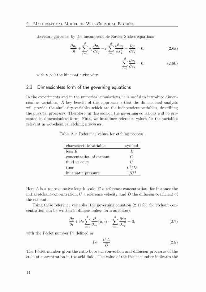
Table 2.1: Reference values for etching process.
characteristic variable symbol
length L
concentration of etchant C
fluid velocity U
time L2/D
kinematic pressure 1/U2
Here L is a representative length scale, C a reference concentration, for instance the
initial etchant concentration, U a reference velocity, and D the diffusion coefficient of
the etchant.
Using these reference variables, the governing equation (2.1) for the etchant con-
centration can be written in dimensionless form as follows:
∂c
∂t+ Pe
d∑
i=1
∂
∂xi
(uic
)−
d∑
i=1
∂2c
∂x2i
= 0, (2.7)
with the Peclet number Pe defined as
Pe =U L
D. (2.8)
The Peclet number gives the ratio between convection and diffusion processes of the
etchant concentration in the acid fluid. The value of the Peclet number indicates the
14
2.3. Dimensionless form of the governing equations
type of the etching process we consider. A small Peclet number means that the trans-
port of the etchant is caused by the diffusion process and is called diffusion-controlled
etching, whereas for large Peclet numbers the concentration is influenced by the fluid
flow and is considered convection-dominated etching. In industrial applications, the
Peclet number is generally large: Pe ∼ 104 and the convection dominates the trans-
port of the etchant. The diffusion process is, however, dominant in thin layers close
to the etched surface. For small values of the Peclet number we can neglect the
convection term in (2.7).
In dimensionless form, the boundary condition (2.3) becomes
d∑
i=1
ni∂c
∂xi= −Sh c, (2.9)
with the Sherwood number Sh defined as
Sh =k L
D. (2.10)
Here k is the surface reaction constant of the dissolution process. The Sherwood
number represents the ratio between the amount of etchant that reacts at the surface
and the amount of etchant transported by the diffusion process towards the surface. In
wet-chemical etching processes the Sherwood number can cover a wide range of values
for different applications, ranging from zero to infinity, and has a significant effect on
the shape of the surface. A small Sherwood number means that the etchant which
has reacted on the surface is immediately transported away from the surface, and the
concentration of the etchant near the surface will be the same as the concentration
away from the surface. A large Sherwood number means that the transport of the
etchant away from the surface is slow compared to the dissolution process of the
etchant at the surface. The etching process is controlled by the mass transfer to and
from the surface and the final shape of the surface depends on a combination of the
fluid velocity field and the concentration of the etchant on the surface.
Next, we consider the governing equation for the movement of the boundary de-
scribed by (2.4). Using the reference values in Table 2.1, we can write (2.4) in dimen-
sionless form as follows:
dxs,i
dt= − 1
βni
d∑
j=1
∂c
∂xjnj, for j = 1, . . . , d, (2.11)
with the parameter β defined as
β =D
σsC. (2.12)
Here σs is the constant defined in (2.5). The parameter β is a measure for the
velocity by which the etched surface moves. When β is very large (β ≫ 1) the surface
moves very slowly. Typical values of β for a few well-known etching systems are
15
2. Mathematical Model of Wet-Chemical Etching
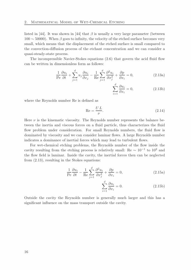
listed in [44]. It was shown in [44] that β is usually a very large parameter (between
100 ∼ 50000). When β goes to infinity, the velocity of the etched surface becomes very
small, which means that the displacement of the etched surface is small compared to
the convection-diffusion process of the etchant concentration and we can consider a
quasi-steady-state process.
The incompressible Navier-Stokes equations (2.6) that govern the acid fluid flow
can be written in dimensionless form as follows:
1
Pe
∂ui
∂t+
d∑
j=1
uj∂ui
∂xj− 1
Re
d∑
j=1
∂2ui
∂x2j
+∂p
∂xi= 0, (2.13a)
d∑
i=1
∂ui
∂xi= 0, (2.13b)
where the Reynolds number Re is defined as
Re =U L
ν. (2.14)
Here ν is the kinematic viscosity. The Reynolds number represents the balance be-
tween the inertia and viscous forces on a fluid particle, thus characterizes the fluid
flow problem under consideration. For small Reynolds numbers, the fluid flow is
dominated by viscosity and we can consider laminar flows. A large Reynolds number
indicates a dominance of inertial forces which may lead to turbulent flows.
For wet-chemical etching problems, the Reynolds number of the flow inside the
cavity resulting from the etching process is relatively small: Re ∼ 10−1 to 102 and
the flow field is laminar. Inside the cavity, the inertial forces then can be neglected
from (2.13), resulting in the Stokes equations:
1
Pe
∂ui
∂t− 1
Re
d∑
j=1
∂2ui
∂x2j
+∂p
∂xi= 0, (2.15a)
d∑
i=1
∂ui
∂xi= 0. (2.15b)
Outside the cavity the Reynolds number is generally much larger and this has a
significant influence on the mass transport outside the cavity.
16
Chapter 3
Discontinuous Galerkin Methods for Elliptic Equations
3.1 Introduction
Discontinuous Galerkin (DG) methods have a number of interesting features which
make them attractive for the solution of the transport equations describing wet-
chemical etching. As outlined in Chapter 1, in particular space-time DG methods
are promising and will receive significant attention in the next two chapters. The
key feature of DG methods is that they use basis functions which are only weakly
coupled to the basis functions in neighboring elements. This makes DG methods
ideally suited for higher order accurate discretizations on unstructured meshes, mesh
adaptation and parallel computing. In this chapter, we will provide an introduction
to the main aspects of DG methods using second-order elliptic partial differential
equations as an example. We will introduce the main techniques frequently used in
the subsequent chapters and also discuss some simple model problems to highlight
certain features of DG methods, including their usefulness for adaptation.
DG methods have been around for quite some time. The first DG method was
introduced in 1973 by Reed and Hill [51] for hyperbolic equations, and since then
there have been major developments in DG methods for first-order hyperbolic partial
differential equations. In particular, the work of Cockburn and Shu has been of
great importance. For a survey, see [18, 19]. At the same time DG methods were
independently proposed for elliptic and parabolic partial differential equations, see
for example [3, 28, 67]. Based on the term added to stabilize the discretization, these
DG methods were usually called interior penalty (IP) methods. The interior penalty
method has, however, a mesh dependent constant which needs to be properly chosen
to ensure stability and is considerably more complicated than continuous Galerkin
(CG) methods, which initially have been applied much more frequently.
In recent years, DG methods have attracted significant attention resulting in many
applications. At first, many researches were dedicated to the development of DG
methods for nonlinear hyperbolic equations, especially for dealing with discontin-
17
3. DGFEM for Elliptic Equations
uous solutions and shock capturing [17]. The excellent results obtained with DG
methods for hyperbolic problems drew the attention from several researchers which
extended the DG discretizations to the more complex fluid flow problems in which,
although the convection still dominates the problem, diffusion should also be taken
into account. An important step forward in combining convection and diffusion in
a DG discretization were the results of Bassi and Rebay [6] for the compressible
Navier-Stokes equations. These equations are rewritten as a first-order system, af-
ter which the DG discretization technique is applied. The approach of Bassi and
Rebay, however, suffered from a weak instability and during the same time several
other approaches were put forward. Important contributions are from Baumann and
Oden [9, 10] which proposed a DG algorithm without free parameters for elliptic par-
tial differential equations and also applied this technique to the convection-diffusion
equation and the compressible Navier-Stokes equations. This algorithm is, however,
suboptimal in accuracy and not stable for linear polynomials. An alternative method
is provided by the Local Discontinuous Galerkin (LDG) method, developed by Cock-
burn and Shu [16] as an extension to the method of Bassi and Rebay. This method is
suitable for a wide range of partial differential equations and has gained considerable
popularity in recent years. The convergence of the LDG method for elliptic problems
on arbitrary and Cartesian meshes is studied in [14] and [20]. An overview of all DG
methods developed so far for elliptic partial differential equations, together with a
unified analysis, can be found in [4]. Motivated by the nice results obtained with DG
methods for elliptic and hyperbolic problems, they have been recently extended to
the incompressible Navier-Stokes equations. The LDG method is used in [21] for the
Stokes equations, and subsequently extended to the Oseen equations in [23], and the
incompressible Navier-Stokes equations in [24]. An analysis of several DG techniques
applied to the Stokes equations is provided in [54, 55].
In the remaining part of this chapter we first introduce the div-grad equation as a
model problem in Section 3.2 and the finite element spaces in Section 3.3. Next, we
describe in Section 3.4 the main steps to derive a DG discretization for second-order
elliptic partial differential equations. Finally, an adaptation technique applied to the
DG discretization is discussed in Section 3.5. In addition, both in Sections 3.4 and
3.5, several aspects of DG methods will be demonstrated with some simple numerical
experiments.
3.2 Model problem
As an introduction to the discontinuous Galerkin methods discussed in Chapters 4
and 5, we describe in this chapter the main steps of deriving a DG discretization for
second order elliptic partial differential equations using the div-grad equation as a
model problem.
Let Ω ⊂ Rd, d = 1, 2, or 3, be a computational domain with boundary ∂Ω. The
18
3.3. FE spaces and trace operators
boundary is partitioned as ∂Ω = ∂ΩD ∪ ∂ΩN , with ∂ΩD ∩ ∂ΩN = ∅ and ∂ΩD has a
nonzero measure. Introducing the notation ∇ for the spatial gradient operator in Rd,
defined as ∇ =(
∂∂x1
, . . . , ∂∂xd
), we consider the following boundary value problem
−∇ · (a∇φ) = f in Ω, (3.1)
with a = aijdi,j=1 a symmetric positive definite matrix and f a given function on
Ω. We supplement (3.1) with the boundary conditions
φ = bD on ∂ΩD, n · (a∇φ) = bN on ∂ΩN , (3.2)
where bD and bN are given functions defined on ∂ΩD and ∂ΩN , respectively, and n
the unit outward normal vector on ∂Ω. As discussed in [4], it is beneficial for the DG
discretization to rewrite the second order partial differential equation (3.1) as a first
order system of equations by introducing an auxiliary variable λ = ∇φ, such that
(3.1) is written as
λ = a∇φ, (3.3a)
−∇ · λ = f. (3.3b)
3.3 Finite element spaces and trace operators
In this section we define the finite element spaces for the DG discretization for the
elliptic equation (3.1) and the trace operators necessary to account for the discontinu-
ity of the basis functions across the element faces. Before doing that, we first discuss
the partitioning of the computational domain into elements.
The computational domain Ω is partitioned into N elements K. The tessellation
Th = K of Ω is defined as
Th := Kj |N⋃
j=1
Kj = Ω and Kj ∩Kj′ = ∅ if j 6= j′, 1 ≤ j, j′ ≤ N.
In this chapter we assume that each element K ∈ Th is an affine image of a fixed
master element K; i.e., K = FK(K) for all K ∈ Th, where K is either the open unit
simplex or the open unit hypercube in Rd. This assumption can be relaxed by using
a composition of two mappings discussed later in Chapter 4. The boundary of each
element is denoted by ∂K, and the outward normal vector on ∂K is denoted by nK .
The radius of the smallest sphere containing each element K is denoted by hK .
We consider several sets of faces. The set of all faces S in Ω is denoted with F ,
the set of all interior faces in Ω with FI , and the set of all boundary faces on ∂Ω
with Fbnd. Two sets of boundary faces are defined as follows. The set of faces with a
Dirichlet boundary condition is denoted as FD, while the set of faces with a Neumann
19
3. DGFEM for Elliptic Equations
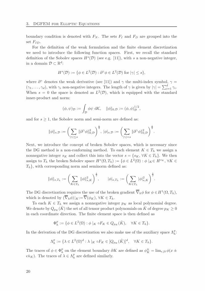
boundary condition is denoted with FN . The sets FI and FD are grouped into the
set FID.
For the definition of the weak formulation and the finite element discretization
we need to introduce the following function spaces. First, we recall the standard
definition of the Sobolev spaces Hs(D) (see e.g. [11]), with s a non-negative integer,
in a domain D ⊂ Rd:
Hs(D) := φ ∈ L2(D) : ∂γφ ∈ L2(D) for |γ| ≤ s,
where ∂γ denotes the weak derivative (see [11]) and γ the multi-index symbol, γ =
(γ1, . . . , γd), with γi non-negative integers. The length of γ is given by |γ| = ∑di=1 γi.
When s = 0 the space is denoted as L2(D), which is equipped with the standard
inner-product and norm:
(φ, ψ)D :=
∫
Dφψ dK, ‖φ‖0,D := (φ, φ)
1/2D ,
and for s ≥ 1, the Sobolev norm and semi-norm are defined as:
‖φ‖s,D :=
(∑
|γ|≤s
‖∂γφ‖20,D
) 12
, |φ|s,D :=
(∑
|γ|=s
‖∂γφ‖20,D
) 12
.
Next, we introduce the concept of broken Sobolev spaces, which is necessary since
the DG method is a non-conforming method. To each element K ∈ Th we assign a
nonnegative integer sK and collect this into the vector s = sK , ∀K ∈ Th. We then
assign to Th the broken Sobolev space Hs(Ω, Th) := φ ∈ L2(Ω) : φ |K∈ HsK , ∀K ∈Th, with corresponding norm and seminorm defined as:
‖φ‖s,Th:=
(∑
K∈Th
‖φ‖2s,K
) 12
, |φ|s,Th:=
(∑
K∈Th
|φ|2s,K
) 12
.
The DG discretization requires the use of the broken gradient ∇hφ for φ ∈H1(Ω, Th),
which is denoted by (∇hφ) |K :=∇(φK), ∀K ∈ Th.
To each K ∈ Th we assign a nonnegative integer pK as local polynomial degree.
We denote byQpK(K) the set of all tensor product polynomials on K of degree pK ≥ 0
in each coordinate direction. The finite element space is then defined as
Φph := φ ∈ L2(Ω) : φ |K FK ∈ QpK
(K), ∀K ∈ Th.
In the derivation of the DG discretization we also make use of the auxiliary space Λph:
Λph := λ ∈ L2(Ω)d : λ |K FK ∈ [QpK
(K)]d, ∀K ∈ Th.
The traces of φ ∈ Φph on the element boundary ∂K are defined as φ±K = limǫ↓0 φ(x±
ǫnK). The traces of λ ∈ Λph are defined similarly.
20
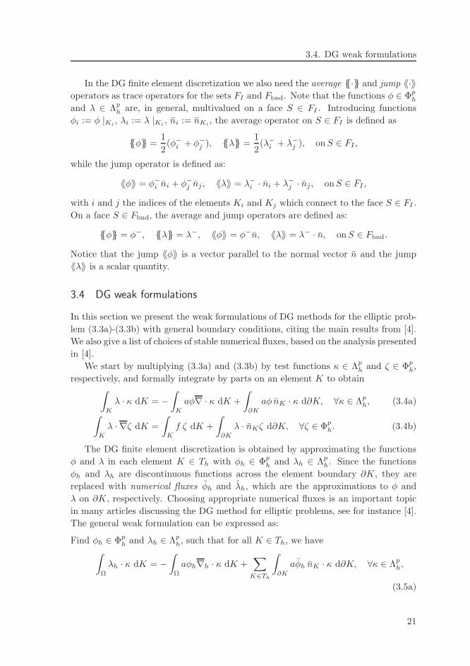
3.4. DG weak formulations
In the DG finite element discretization we also need the average · and jump 〈〈·〉〉operators as trace operators for the sets FI and Fbnd. Note that the functions φ ∈ Φp
h
and λ ∈ Λph are, in general, multivalued on a face S ∈ FI . Introducing functions
φi := φ |Ki, λi := λ |Ki
, ni := nKi, the average operator on S ∈ FI is defined as
φ =1
2(φ−i + φ−j ), λ =
1
2(λ−i + λ−j ), onS ∈ FI ,
while the jump operator is defined as:
〈〈φ〉〉 = φ−i ni + φ−j nj , 〈〈λ〉〉 = λ−i · ni + λ−j · nj , onS ∈ FI ,
with i and j the indices of the elements Ki and Kj which connect to the face S ∈ FI .
On a face S ∈ Fbnd, the average and jump operators are defined as:
φ = φ−, λ = λ−, 〈〈φ〉〉 = φ−n, 〈〈λ〉〉 = λ− · n, onS ∈ Fbnd.
Notice that the jump 〈〈φ〉〉 is a vector parallel to the normal vector n and the jump
〈〈λ〉〉 is a scalar quantity.
3.4 DG weak formulations
In this section we present the weak formulations of DG methods for the elliptic prob-
lem (3.3a)-(3.3b) with general boundary conditions, citing the main results from [4].
We also give a list of choices of stable numerical fluxes, based on the analysis presented
in [4].
We start by multiplying (3.3a) and (3.3b) by test functions κ ∈ Λph and ζ ∈ Φp
h,
respectively, and formally integrate by parts on an element K to obtain∫
K
λ · κ dK = −∫
K
aφ∇ · κ dK +
∫
∂K
aφ nK · κ d∂K, ∀κ ∈ Λph, (3.4a)
∫
K
λ · ∇ζ dK =
∫
K
f ζ dK +
∫
∂K
λ · nKζ d∂K, ∀ζ ∈ Φph. (3.4b)
The DG finite element discretization is obtained by approximating the functions
φ and λ in each element K ∈ Th with φh ∈ Φph and λh ∈ Λp
h. Since the functions
φh and λh are discontinuous functions across the element boundary ∂K, they are
replaced with numerical fluxes φh and λh, which are the approximations to φ and
λ on ∂K, respectively. Choosing appropriate numerical fluxes is an important topic
in many articles discussing the DG method for elliptic problems, see for instance [4].
The general weak formulation can be expressed as:
Find φh ∈ Φph and λh ∈ Λp
h, such that for all K ∈ Th, we have∫
Ω
λh · κ dK = −∫
Ω
aφh∇h · κ dK +∑
K∈Th
∫
∂K
aφh nK · κ d∂K, ∀κ ∈ Λph,
(3.5a)
21
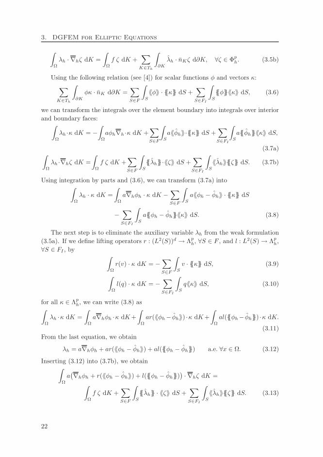
3. DGFEM for Elliptic Equations
∫
Ω
λh · ∇hζ dK =
∫
Ω
f ζ dK +∑
K∈Th
∫
∂K
λh · nKζ d∂K, ∀ζ ∈ Φph. (3.5b)
Using the following relation (see [4]) for scalar functions φ and vectors κ:
∑
K∈Th
∫
∂K
φκ · nK d∂K =∑
S∈F
∫
S
〈〈φ〉〉 · κ dS +∑
S∈FI
∫
S
φ〈〈κ〉〉 dS, (3.6)
we can transform the integrals over the element boundary into integrals over interior
and boundary faces:∫
Ω
λh ·κ dK = −∫
Ω
aφh∇h ·κ dK +∑
S∈F
∫
S
a〈〈φh〉〉·κ dS +∑
S∈FI
∫
S
aφh〈〈κ〉〉 dS,
(3.7a)∫
Ω
λh ·∇hζ dK =
∫
Ω
f ζ dK +∑
S∈F
∫
S
λh·〈〈ζ〉〉 dS +∑
S∈FI
∫
S
〈〈λh〉〉ζ dS. (3.7b)
Using integration by parts and (3.6), we can transform (3.7a) into∫
Ω
λh · κ dK =
∫
Ω
a∇hφh · κ dK −∑
S∈F
∫
S
a〈〈φh − φh〉〉 · κ dS
−∑
S∈FI
∫
S
aφh − φh〈〈κ〉〉 dS. (3.8)
The next step is to eliminate the auxiliary variable λh from the weak formulation
(3.5a). If we define lifting operators r : (L2(S))d → Λph, ∀S ∈ F , and l : L2(S)→ Λp
h,
∀S ∈ FI , by∫
Ω
r(v) · κ dK = −∑
S∈F
∫
S
v · κ dS, (3.9)
∫
Ω
l(q) · κ dK = −∑
S∈FI
∫
S
q〈〈κ〉〉 dS, (3.10)
for all κ ∈ Λph, we can write (3.8) as
∫
Ω
λh ·κ dK =
∫
Ω
a∇hφh ·κ dK+
∫
Ω
ar(〈〈φh− φh〉〉) ·κ dK+
∫
Ω
al(φh− φh) ·κ dK.
(3.11)
From the last equation, we obtain
λh = a∇hφh + ar(〈〈φh − φh〉〉) + al(φh − φh) a.e. ∀x ∈ Ω. (3.12)
Inserting (3.12) into (3.7b), we obtain∫
Ω
a(∇hφh + r(〈〈φh − φh〉〉) + l(φh − φh)
)· ∇hζ dK =
∫
Ω
f ζ dK +∑
S∈F
∫
S
λh · 〈〈ζ〉〉 dS +∑
S∈FI
∫
S
〈〈λh〉〉ζ dS. (3.13)
22
3.4. DG weak formulations
The DG weak formulation for the div-grad equation (3.1) then can be written as:
Find a φh ∈ Φph, such that the following relation is satisfied for all ζ ∈ Φp
h:
B(φh, ζ) =
∫
Ω
f ζ dK, (3.14)
where using (3.9)-(3.10), B(φh, ζ) are defined as:
B(φh, ζ) :=
∫
Ω
a∇hφh · ∇hζ dK −∑
S∈F
∫
S
(a〈〈φh − φh〉〉 · ∇hζ + λh · 〈〈ζ〉〉
)dS
−∑
S∈FI
∫
S
(aφh − φh〈〈∇hζ〉〉+ 〈〈λh〉〉ζ
)dS. (3.15)
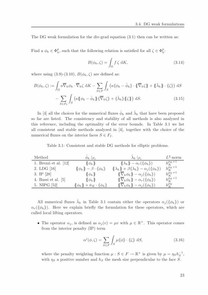
In [4] all the choices for the numerical fluxes φh and λh that have been proposed
so far are listed. The consistency and stability of all methods is also analyzed in
this reference, including the optimality of the error bounds. In Table 3.1 we list
all consistent and stable methods analyzed in [4], together with the choice of the
numerical fluxes on the interior faces S ∈ FI .
Table 3.1: Consistent and stable DG methods for elliptic problems.
Method φh |FIλh |FI
L2-norm
1. Brezzi et al. [12] φh λh − αr(〈〈φh〉〉) hpK+1K
2. LDG [16] φh − β · 〈〈φh〉〉 λh+ β〈〈λh〉〉 − αj(〈〈φh〉〉) hpK+1K
3. IP [28] φh ∇hφh − αj(〈〈φh〉〉) hpK+1K
4. Bassi et al. [5] φh ∇hφh − αr(〈〈φh〉〉) hpK+1K
5. NIPG [52] φh+ nK · 〈〈φh〉〉 ∇hφh − αj(〈〈φh〉〉) hpK
K
All numerical fluxes λh in Table 3.1 contain either the operators αj(〈〈φh〉〉) or
αr(〈〈φh〉〉). Here we explain briefly the formulation for these operators, which are
called local lifting operators.
• The operator αj , is defined as αj(v) = µv with µ ∈ R+. This operator comes
from the interior penalty (IP) term
αj(φ, ζ) =∑
S∈F
∫
S
µ〈〈φ〉〉 · 〈〈ζ〉〉 dS, (3.16)
where the penalty weighting function µ : S ∈ F → R+ is given by µ = ηSh−1S ,
with ηS a positive number and hS the mesh size perpendicular to the face S.
23
3. DGFEM for Elliptic Equations
• The operator αr(v), is defined as αr(v) = −ηSrS(v) on a face S ∈ FI and
as αr(v) = −ηSrS(v) + ηSrS(bDn) on a face S ∈ FD. On a face S ∈ FN
this operator αr(v) is equal to zero. For all κ ∈ Λph, the local lifting operator
rS : (L2(S))d → Λph is given by
∫
Ω
rS(v) · κ dK = −∫
S
v · κ dS, on S ∈ FI , (3.17)
∫
Ω
rS(v) · κ dK = −∫
S
v · κ dS, on S ∈ FD. (3.18)
Note that rS(v) vanishes outside the union of the one or two elements connected
to the face S and that r(v) =∑
S∈F rS(v) for any K ∈ Th.
We state here the main conclusions based on the analysis given in [4]. The Methods
1-4 in Table 3.1 are consistent, adjoint consistent, stable (under certain conditions on
the parameters µ and ηs) and have optimal rates of convergence hpK+1K in the L2-
norm. Method 5 is consistent and stable (under similar conditions on µ, ηS), but is
not adjoint consistent and has suboptimal rates of convergence hpK
K in the L2-norm.
All methods in Table 3.1 have a local lifting operator in their formulation, either of the
form αj or αr. This fact indicates that the lifting operator plays an important role in
the DG method (more precisely to the stability of the methods). It is also concluded
in [4] that DG methods whose numerical fluxes λh are independent of λh (Methods
3-5 in Table 3.1) produce stiffness matrices with a smaller number of non-zero entries.
This makes that matrices resulting from the DG discretization with Methods 3-5 are
more sparse than the matrices resulting from the DG discretization with Methods
1-2.
Considering several aspects of the numerical discretization, such as consistency,
stability, optimal convergence, and sparsity of the resulting matrices, Methods 3-4 in
Table 3.1 are good candidates for further study. Method 3, however, uses the local
lifting operator αj and the parameter µ in this operator depends on h−1S , the mesh
size perpendicular to the face S on which this operator acts, which is not easy to
define on general anisotropic meshes. Method 4, meanwhile, uses the local lifting
operator αr, and this operator only depends on a parameter ηS which is independent
of the element size. Based on this fact, we choose Method 4 for the extension of the
DG formulation to space-time problems, which will be discussed in Chapters 4 and 5.
We discuss now in detail the bilinear form B(·, ·) for Method 4, which is first
introduced in [5], and later discussed in [7, 12]. For the general boundary conditions
(3.2), the Bassi et al. method [5] uses the following numerical fluxes:
φh = φh onS ∈ FI ,
φh = bD onS ∈ FD, (3.19)
φh = φh onS ∈ FN ,
24
3.5. Adaptation
and:
λh = ∇hφh+ ηSrS(〈〈φh〉〉) onS ∈ FI ,
λh = ∇hφh + ηSrS(〈〈φh〉〉)− ηSrS(bDn) onS ∈ FD, (3.20)
λh · n = bN onS ∈ FN .
Substituting (3.19)-(3.20) into (3.15), we obtain
B(φh, ζ) :=
∫
Ω
a∇hφh ·∇hζ dK
−∑
S∈FID
∫
S
a(〈〈φh〉〉·∇hζ+ ∇hφh·〈〈ζ〉〉+ ηSrS(〈〈φh〉〉)·〈〈ζ〉〉
)dS
+∑
S∈FD
∫
S
a(bDn·∇hζ + ηSrS(bDn)·nζ
)dS −
∑
S∈FN
∫
S
bNζ dS. (3.21)
It is shown in [4, 12] that the bilinear form (3.21) is stable when the constant parameter
ηS is chosen such that ηS > NS , with NS the number of faces on each element.
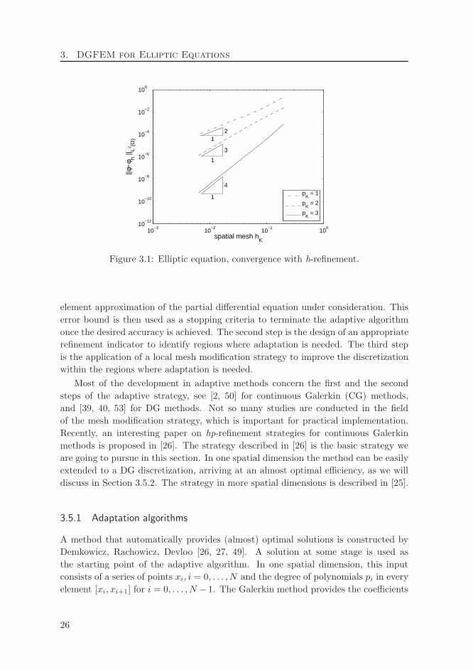
We complete this section with presenting some simple numerical experiments in
one spatial dimension to demonstrate theoretically predicted rate of convergence of
the DG discretization Method 4, O(hpK+1K ) in the L2-norm (see the last column in
Table 3.1).
We consider the elliptic equation (3.1) in Ω = (0, 1) with a = 1. The right hand
side f and the Dirichlet boundary condition bD are chosen such that the exact solution
is:
φ(x) = sin(2πx).
We show the rates of convergence of the error in the L2-norm for successively finer
meshes and increasing polynomial degrees. The results are given in Fig. 3.1. This
figure shows that the error in the L2-norm converges at the optimal rate hpK+1K , which
is predicted by the theoretical estimates given in the last column in Table 3.1.
3.5 Adaptation
One of features of DG methods is their suitability for adaptation. In the field of
adaptation several different strategies are distinguished: h-refinement by locally re-
fining the mesh size, p-refinement by locally increasing the polynomial degree, and
hp-refinement, which is a combination of h and p-refinement.
The search for optimal adaptation strategies has a long history in the development
of finite element methods. A series of memorable papers on h-adaptivity, p-adaptivity,
and hp-adaptivity has been written by Babuska and Gui in 1986, see [34, 35, 36].
In general, the construction of an adaptive strategy involves three main steps
[39]. The first one is the derivation of a sharp a posteriori error bound for the finite
25
3. DGFEM for Elliptic Equations
10−3
10−2
10−1
100
10−12
10−10
10−8
10−6
10−4
10−2
100
spatial mesh hK
||φ−
φ h ||L2 (Ω
) 1
1
1
2
3
4p
K = 1
pK = 2
pK = 3
Figure 3.1: Elliptic equation, convergence with h-refinement.
element approximation of the partial differential equation under consideration. This
error bound is then used as a stopping criteria to terminate the adaptive algorithm
once the desired accuracy is achieved. The second step is the design of an appropriate
refinement indicator to identify regions where adaptation is needed. The third step
is the application of a local mesh modification strategy to improve the discretization
within the regions where adaptation is needed.
Most of the development in adaptive methods concern the first and the second
steps of the adaptive strategy, see [2, 50] for continuous Galerkin (CG) methods,
and [39, 40, 53] for DG methods. Not so many studies are conducted in the field
of the mesh modification strategy, which is important for practical implementation.
Recently, an interesting paper on hp-refinement strategies for continuous Galerkin
methods is proposed in [26]. The strategy described in [26] is the basic strategy we
are going to pursue in this section. In one spatial dimension the method can be easily
extended to a DG discretization, arriving at an almost optimal efficiency, as we will
discuss in Section 3.5.2. The strategy in more spatial dimensions is described in [25].
3.5.1 Adaptation algorithms
A method that automatically provides (almost) optimal solutions is constructed by
Demkowicz, Rachowicz, Devloo [26, 27, 49]. A solution at some stage is used as
the starting point of the adaptive algorithm. In one spatial dimension, this input
consists of a series of points xi, i = 0, . . . , N and the degree of polynomials pi in every
element [xi, xi+1] for i = 0, . . . , N − 1. The Galerkin method provides the coefficients
26
3.5. Adaptation
of each individual polynomial. The adaptive algorithm for one spatial dimension can
be summarized in the following algorithm.
Algorithm 3.1 1D Adaptive algorithm from [26].
(1) Compute the solution u∗ on a globally refined hp grid, i.e., the solution on a twice
finer grid, with the polynomial degree in every element raised by one. So within
an old element [xi, xi+1], u∗ can be represented by two polynomials of degree
pi + 1, namely on the element [xi, (xi + xi+1)/2] and on [(xi + xi+1)/2, xi+1].
Hence the total number of the degrees of freedom on a refined grid becomes
2(pi + 2).
(2) Solve the following (equidistant) interpolation problems in each old element
[xi, xi+1]:
(i) interpolate u∗ on [xi, xi+1] with one polynomial of degree pi + 1, i.e., the
number of the degrees of freedom is equal to pi + 2.
(ii) interpolate u∗ on both elements [xi, (xi +xi+1)/2] and [(xi +xi+1)/2, xi+1]
with two polynomials whose degrees add up to pi, i.e. the number of the
degrees of freedom equals pi,1 + 1 + pi,2 + 1 = pi + 2, with pi,1, pi,2 are
the polynomial degrees of the two subintervals. The choice for a pair of
polynomial degrees is: (pi − 1, 1), (pi − 2, 2), ..., (1, pi − 1).
(3) For each choice in Steps (2.i) and (2.ii), we compute the error ǫi, defined as:
ǫi = ‖u∗ − uchoice‖0,K ,
and the best choice is the one that gives minimal ǫi. This choice is stored,
together with the corresponding ǫi.
(4) The elements i with error ǫi larger than a given tolerance are refined with the
adaptation technique (h or p-refinement) chosen in Step (3).
There are several remarks regarding Algorithm 3.1. First, the strategy requires
first finding a much better reference solution u∗ of the problem, and then locally in
every element the best approximation of u∗ is constructed using interpolation with
a smaller number of coefficients. Indeed, in element i, the solution u∗ has 2(pi + 2)
degrees of freedom, whereas each approximation in Step (2) has pi + 2 degrees of
freedom. The degrees of freedom on a refined element are increased by one, no matter
what choice has been made in Step (2).
For the DG discretization the basic strategy is slightly modified. The interpolation
and the L2-norm computations are replaced with the computation of the L2-norm of
the approximation. (Using Legendre polynomials as basis functions, Step (2) reduces
to taking a few inner-products). The following algorithm is then applied for the DG
discretization.
27
3. DGFEM for Elliptic Equations
Algorithm 3.2 Modified 1D adaptation algorithm.
(1) Compute the solution u∗ on a globally refined hp grid. Within an old element
[xi, xi+1], u∗ can be represented by two polynomials of degree pi +1, namely on
the element [xi, (xi + xi+1)/2] and on [(xi + xi+1)/2, xi+1].
(2) In each old element [xi, xi+1] compute the following approximation errors:
(i) The L2-approximation of u∗ on [xi, xi+1] with one polynomial of degree
pi + 1.
(ii) The L2-approximation of u∗ on both elements [xi, (xi +xi+1)/2] and [(xi +
xi+1)/2, xi+1] with two polynomials whose degrees add up to pi. The choice
for a pair of the polynomial degrees is: (pi, 0), ..., (0, pi).
(3) In each element determine the best approximation from Steps (2.i) and (2.ii),
that is the one with the smallest ǫi, with ǫi defined in Algorithm 3.1.
(4) The elements i with the error ǫi larger than a given tolerance are refined with
the adaptation technique (either h or -p refinement) chosen in Step (3).
3.5.2 The efficiency of the method
We test the described method on the following model problem:
d
dx
(
xβ dφ(x)
dx
)
= 2− β, φ(0) = 0, φ(1) = 1, (3.22)
which has the analytic solution: φ(x) = x2−β . This solution is chosen based on the
discussion in [34, 35, 36] which specifies theoretically the results of an optimal hp-
refinement strategy. This theoretical result therefore provides a benchmark for every
hp-adaptive method. The characterization of an optimal solution to problem (3.22)
discussed in [34, 35, 36] can be summarized as follows:
• The error ǫ as a function of N , with N the total degrees of freedom, shows an
exponential decay:
ǫ ≤ Ce−γ√
N (3.23)
with γ a positive constant.
• The optimal mesh is a graded one, i.e.,
hi+1 = λhi, (3.24)
with i the mesh index counted from x = 0, which means that away from the
singularity the mesh stretches with a factor of λ. The optimal value for λ is
given as: λ = λ∗ = 1/(√
2− 1)2 ≈ 6.
28
3.5. Adaptation
• The polynomial degree increases away from the singularity with the following
formula:
pi = ⌈µi⌉, (3.25)
with i the mesh index counted from x = 0 and µ a positive constant.
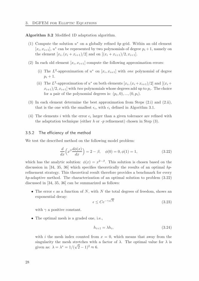
The adaptive method described in Algorithm 3.2 is implemented for problem (3.22)
with β = 1/3, and the results show a very good approximation of the optimal solution
and the final grid resulting from the adaptation. The local degree of the polynomials
in each element is shown in Fig. 3.2.
index interval
pol
ynom
iald
egre
e
0 10 20 301
2
3
4
5
6
7
8
9
10
Figure 3.2: Local polynomial degree for problem (3.22) with β = 1/3, using Algorithm
3.2.
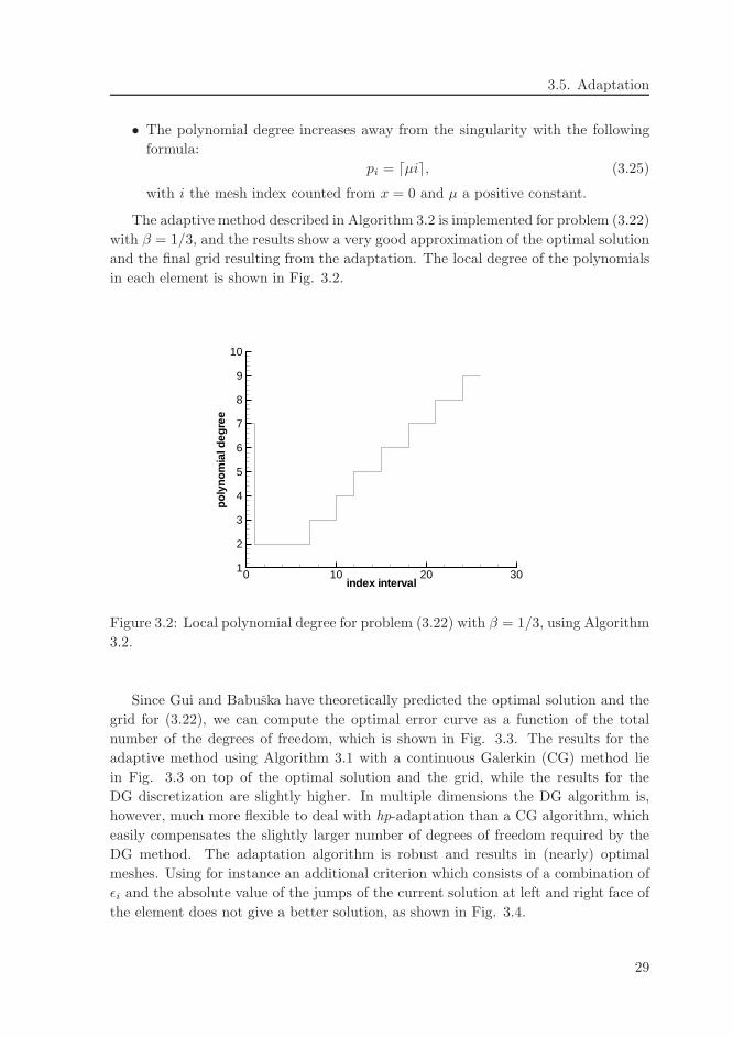
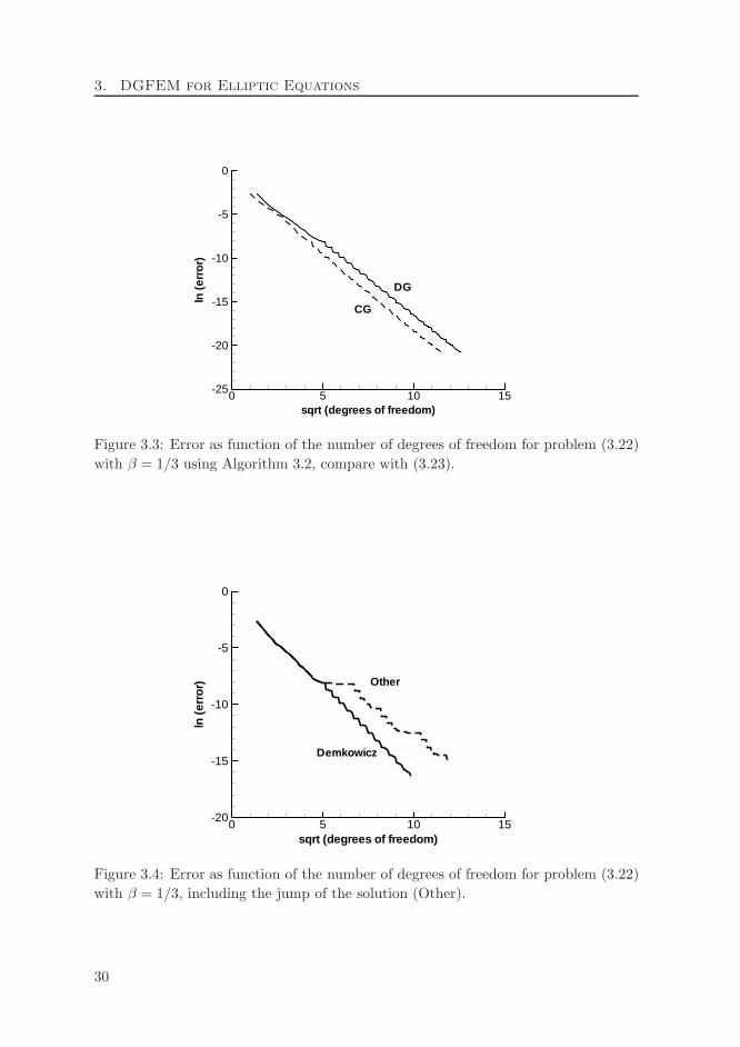
Since Gui and Babuska have theoretically predicted the optimal solution and the
grid for (3.22), we can compute the optimal error curve as a function of the total
number of the degrees of freedom, which is shown in Fig. 3.3. The results for the
adaptive method using Algorithm 3.1 with a continuous Galerkin (CG) method lie
in Fig. 3.3 on top of the optimal solution and the grid, while the results for the
DG discretization are slightly higher. In multiple dimensions the DG algorithm is,
however, much more flexible to deal with hp-adaptation than a CG algorithm, which
easily compensates the slightly larger number of degrees of freedom required by the
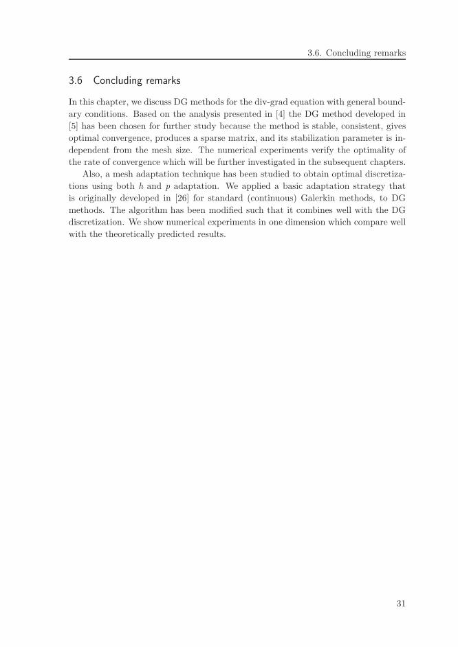
DG method. The adaptation algorithm is robust and results in (nearly) optimal
meshes. Using for instance an additional criterion which consists of a combination of
ǫi and the absolute value of the jumps of the current solution at left and right face of
the element does not give a better solution, as shown in Fig. 3.4.
29
3. DGFEM for Elliptic Equations
sqrt (degrees of freedom)
ln(e
rro
r)
0 5 10 15-25
-20
-15
-10
-5
0
CG
DG
Figure 3.3: Error as function of the number of degrees of freedom for problem (3.22)
with β = 1/3 using Algorithm 3.2, compare with (3.23).
sqrt (degrees of freedom)
ln(e
rror
)
0 5 10 15-20
-15
-10
-5
0
Demkowicz
Other
Figure 3.4: Error as function of the number of degrees of freedom for problem (3.22)
with β = 1/3, including the jump of the solution (Other).
30
3.6. Concluding remarks
3.6 Concluding remarks
In this chapter, we discuss DG methods for the div-grad equation with general bound-
ary conditions. Based on the analysis presented in [4] the DG method developed in
[5] has been chosen for further study because the method is stable, consistent, gives
optimal convergence, produces a sparse matrix, and its stabilization parameter is in-
dependent from the mesh size. The numerical experiments verify the optimality of
the rate of convergence which will be further investigated in the subsequent chapters.
Also, a mesh adaptation technique has been studied to obtain optimal discretiza-
tions using both h and p adaptation. We applied a basic adaptation strategy that
is originally developed in [26] for standard (continuous) Galerkin methods, to DG
methods. The algorithm has been modified such that it combines well with the DG
discretization. We show numerical experiments in one dimension which compare well
with the theoretically predicted results.
31

Chapter 4
A Space-Time Discontinuous Galerkin Method for the
Advection-Diffusion Equation in Time-Dependent
Domains
4.1 Introduction
Wet-chemical etching processes require a finite element method which can efficiently
deal with deforming elements to accommodate for the movement of the etching cav-
ity boundary. In addition, thin boundary layers and singularities must be captured
which can be done efficiently with mesh adaptation using either mesh refinement
(h-adaptation) or adjustment of the polynomial degree (p-refinement). The space-
time DG method, which simultaneously discretizes the equations in space and time,
provides the necessary flexibility to deal both with time deforming meshes and hp-
adaptation, and is an excellent technique for this type of problems. In this chapter
we discuss the space-time DG discretization for the advection-diffusion equation in a
time-dependent domain, which is the governing equation for the concentration of the
etchant (2.1). The material is taken from [61].
First, the advection-diffusion equation is transformed to the space-time framework
in a rather general setting. This will allow the extension of the mathematical model
to anisotropic etching processes. After a description of the construction of space-
time elements and the introduction of the function spaces and trace operators in
Section 4.3, we give a complete derivation of the space-time DG discretization for
the advection-diffusion equation in Section 4.4. This section is completed with the
Arbitrary Lagrangian Eulerian (ALE) formulation of the space-time DG discretization
as the latter formulation is useful for actual implementation of the discretization.
We then analyze the stability and the uniqueness of the numerical solution of
the space-time DG discretization in Section 4.5. We also give error estimates and
prove hp convergence of the space-time DG discretization in Section 4.6. Some simple
numerical experiments are presented in Section 4.7 to verify the analysis.
33
4. A Space-Time DGFEM for Advection-Diffusion
4.2 The advection-diffusion equation
In this section we consider the advection-diffusion equation in the usual form and in
the space-time framework. Let Ωt be an open, bounded domain in Rd, with d the
number of spatial dimensions. The closure of Ωt is Ωt and the boundary of Ωt is
denoted by ∂Ωt. The subscript t denotes the domain at time t as we consider the
geometry of the spatial domain to be time-dependent. The outward normal vector
to ∂Ωt is denoted by n = (n1, . . . , nd). Denoting x = (x1, . . . , xd) as the spatial
variables, we consider the time-dependent advection-diffusion equation:
∂c
∂t+
d∑
i=1
∂
∂xi
(ui(t, x)c
)−
d∑
i,j=1
∂
∂xj
(
Dij(t, x)∂c
∂xi
)
= 0, in Ωt, (4.1)
where u = (u1, . . . , ud) is a vector field whose entries are continuous real-valued
functions on Ωt. Furthermore,D ∈ Rd×d is a symmetric matrix of diffusion coefficients
on Ωt whose entries are continuous real-valued functions. This matrix is positive
definite in Ωt and positive semi-definite on ∂Ωt. Then there exists a symmetric
matrix D⋆ ∈ Rd×d, the matrix square root D⋆ = D1/2, such that
D = D⋆D⋆. (4.2)
In the space-time discretization we directly consider a domain in Rd+1. A point
x ∈ Rd+1 has coordinates (x0, x), with x0 = t representing time. We then define the
space-time domain E ⊂ Rd+1. The boundary of the space-time domain ∂E consists
of the hypersurfaces Ω0 := x ∈ ∂E | x0 = 0, ΩT := x ∈ ∂E | x0 = T , and
Q := x ∈ ∂E | 0 < x0 < T . We reformulate the advection-diffusion equation now
in the space-time framework. First, we introduce the vector function B ∈ Rd+1 and
the symmetric matrix A ∈ R(d+1)×(d+1) as:
B =(1, u
), A =
(0 0
0 D
)
.
Then the advection-diffusion equation (4.1) can be transformed into a space-time
formulation as:
−∇ · (−Bc+A∇c) = 0 in E , (4.3)
where ∇ =(
∂∂x0
, ∂∂x1
, . . . , ∂∂xd
)denotes the gradient operator in Rd+1. Later we will
also use the notation ∇ to denote the spatial gradient operator in Rd, defined as
∇ =(
∂∂x1
, . . . , ∂∂xd
). The unit outward normal vector at ∂E is denoted with n.
As different boundary conditions are imposed on ∂E , we discuss in more detail
the subdivision of ∂E into different parts. The boundary ∂E is divided into disjoint
boundary subsets ΓS ,Γ−, and Γ+, where each subset is defined as follows:
ΓS := x ∈ ∂E : nTDn > 0,Γ− := x ∈ ∂E \ ΓS : B · n < 0, Γ+ := x ∈ ∂E \ ΓS : B · n ≥ 0.
34
4.3. Space-time description, FE spaces and trace operators
The subscript S denotes the part of ∂E where matrix D is symmetric positive definite,
while the subscripts − and + denote the inflow and outflow boundaries, respectively.
We assume that ΓS has a non-zero surface measure. Note that ∂E = ΓS ∪ Γ− ∪ Γ+.
We subdivide ΓS further into two sets: ΓS = ΓDS ∪ ΓM , with ΓDS the part of ΓS
with a Dirichlet boundary condition and ΓM the part of ΓS with a mixed boundary
condition. We also subdivide Γ− into two parts: Γ− = ΓDB ∪Ω0, with ΓDB the part
of Γ− with a Dirichlet boundary condition and Ω0 the part of Γ− with the initial
condition. Note that ΓD = ΓDS ∪ ΓDB ⊂ ∂E is the part of the space-time domain
boundary with a Dirichlet boundary condition. The boundary conditions on different
parts of ∂E are written as
c = c0 on Ω0,
c = gD on ΓD, (4.4)
αc+ n · (A∇c) = gM on ΓM ,
with α ≥ 0 and c0, gD, gM given functions defined on the boundary. There is no
boundary condition imposed on Γ+.
4.3 Space-time description, finite element spaces and trace operators
4.3.1 Definition of space-time slabs, elements and faces
In this section we give a description of the space-time slabs, elements and faces used
in the DG discretization. First, consider the time interval I = [0, T ], partitioned by
an ordered series of time levels t0 = 0 < t1 < . . . < tNt= T . Denoting the nth
time interval as In = (tn, tn+1), we have I = ∪nIn. The length of In is defined as
nt = tn+1− tn. Let Ωtnbe an approximation to the spatial domain Ω at tn for each
n = 0, . . . , Nt. A space-time slab is defined as the domain En = E ∩ (In × Rd) with
boundaries Ωtn, Ωtn+1 and Qn = ∂En \ (Ωtn
∪ Ωtn+1).
We now describe the construction of the space-time elements K in the space-time
slab En. Let the domain Ωtnbe divided into Nn non-overlapping spatial elements
Kn. At tn+1 the spatial elements Kn+1 are obtained by mapping the elements Kn
to their new position. Each space-time element K is obtained by connecting elements
Kn and Kn+1 using linear interpolation in time. A sketch of the space-time slab En
and element K for two spatial dimensions is shown in Fig. 4.1. We denote by hKthe radius of the smallest sphere containing each element K. The element boundary
∂K is the union of open faces of K, which contains three parts Kn,Kn+1, and QnK =
∂K \ (Kn ∪Kn+1). We denote by nK the unit outward space-time normal vector on
∂K. The definition of the space-time domain is completed with the tessellation T nh ,
which consists of all space-time elements in En, and Th = ∪nT nh , which consists of all
space-time elements in E .
35
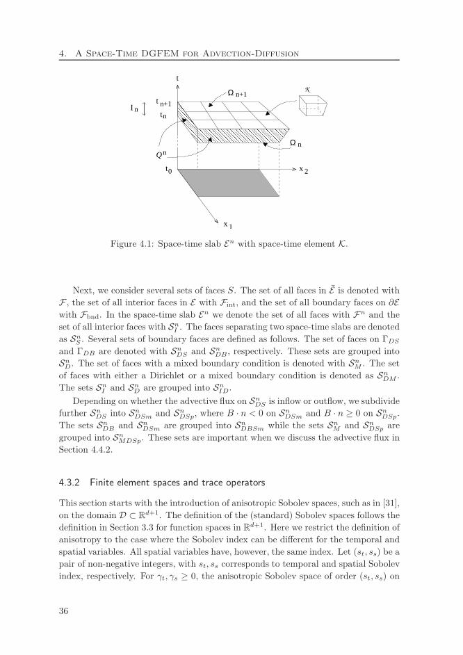
4. A Space-Time DGFEM for Advection-Diffusion
I n
t n+1
tn
t0
Qn
Ω
Ω n
x
tK
x
n+1
2
1
Figure 4.1: Space-time slab En with space-time element K.
Next, we consider several sets of faces S. The set of all faces in E is denoted with
F , the set of all interior faces in E with Fint, and the set of all boundary faces on ∂Ewith Fbnd. In the space-time slab En we denote the set of all faces with Fn and the
set of all interior faces with SnI . The faces separating two space-time slabs are denoted
as SnS . Several sets of boundary faces are defined as follows. The set of faces on ΓDS
and ΓDB are denoted with SnDS and Sn
DB , respectively. These sets are grouped into
SnD. The set of faces with a mixed boundary condition is denoted with Sn
M . The set
of faces with either a Dirichlet or a mixed boundary condition is denoted as SnDM .
The sets SnI and Sn
D are grouped into SnID.
Depending on whether the advective flux on SnDS is inflow or outflow, we subdivide
further SnDS into Sn
DSm and SnDSp, where B · n < 0 on Sn
DSm and B · n ≥ 0 on SnDSp.
The sets SnDB and Sn
DSm are grouped into SnDBSm while the sets Sn
M and SnDSp are
grouped into SnMDSp. These sets are important when we discuss the advective flux in
Section 4.4.2.
4.3.2 Finite element spaces and trace operators
This section starts with the introduction of anisotropic Sobolev spaces, such as in [31],
on the domain D ⊂ Rd+1. The definition of the (standard) Sobolev spaces follows the
definition in Section 3.3 for function spaces in Rd+1. Here we restrict the definition of
anisotropy to the case where the Sobolev index can be different for the temporal and
spatial variables. All spatial variables have, however, the same index. Let (st, ss) be a
pair of non-negative integers, with st, ss corresponds to temporal and spatial Sobolev
index, respectively. For γt, γs ≥ 0, the anisotropic Sobolev space of order (st, ss) on
36
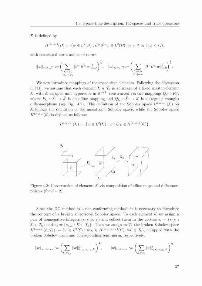
4.3. Space-time description, FE spaces and trace operators
D is defined by
H(st,ss)(D) := w ∈ L2(D) : ∂γt∂γsw ∈ L2(D) for γt ≤ st, |γs| ≤ ss,
with associated norm and semi-norm:
‖w‖st,ss,D :=
(∑
γt≤st
|γs|≤ss
‖∂γt∂γsw‖20,D
) 12
, |w|st,ss,D :=
(∑
γt=st
|γs|=ss
‖∂γt∂γsw‖20,D
) 12
.
We now introduce mappings of the space-time elements. Following the discussion
in [31], we assume that each element K ∈ Th is an image of a fixed master element
K, with K an open unit hypercube in Rd+1, constructed via two mappings QK FK,
where FK : K → K is an affine mapping and QK : K → K is a (regular enough)
diffeomorphism (see Fig. 4.2). The definition of the Sobolev space H(st,ss)(K) on
K follows the definition of the anisotropic Sobolev space, while the Sobolev space
H(st,ss)(K) is defined as follows:
H(st,ss)(K) := w ∈ L2(K) : w QK ∈ H(st,ss)(K).
F
K
K KK
QK
t
x1
x2
1h
∆ tn
h2
Figure 4.2: Construction of elements K via composition of affine maps and diffeomor-
phisms (for d = 2).
Since the DG method is a non-conforming method, it is necessary to introduce
the concept of a broken anisotropic Sobolev space. To each element K we assign a
pair of nonnegative integers (st,K, ss,K) and collect them in the vectors st = st,K :
K ∈ Th and ss = ss,K : K ∈ Th. Then we assign to Th the broken Sobolev space
H(st,ss)(E , Th) := w ∈ L2(E) : w|K ∈ H(st,K,ss,K)(K), ∀K ∈ Th, equipped with the
broken Sobolev norm and corresponding semi-norm, respectively,
‖w‖st,ss,Th:=
(∑
K∈Th
‖w‖2st,K,ss,K,K
) 12
, |w|st,ss,Th:=
(∑
K∈Th
|w|2st,K ,ss,K,K
) 12
.
37
4. A Space-Time DGFEM for Advection-Diffusion
For w ∈ H(1,1)(E , Th), we define the broken gradient ∇hw of w by (∇hw)|K :=
∇(w|K), ∀K ∈ Th.
Now we introduce the finite element spaces associated with the tessellation Th that
will be used in this chapter. To each elementK we assign a pair of nonnegative integers
(pt,K, ps,K) as local polynomial degrees, where the subscripts t and s denote time and
space, and collect them into vectors pt = pt,K : K ∈ Th and ps = ps,K : K ∈ Th.Defining Qpt,K,ps,K
(K) as the set of all tensor-product polynomials on K of degree pt,Kin the time direction and degree ps,K in each spatial coordinate direction, we then
introduce the finite element space of discontinuous piecewise polynomial functions as
W(pt,ps)h := w ∈ L2(E) : w|K QK FK ∈ Q(pt,K,ps,K)(K), ∀K ∈ Th.
In the derivation and analysis of the numerical discretization we also make use of the
auxiliary space Υ(pt,ps)h :
Υ(pt,ps)h = ϕ ∈ L2(E)d+1 : ϕ|K QK FK ∈ [Q(pt,K,ps,K)(K)]d+1, ∀K ∈ Th.
The so called traces of w ∈ W(pt,ps)h on ∂K are defined as: w±
K = limǫ↓0 w(x ± ǫnK).
The traces of ϕ ∈ Υ(pt,ps)h are defined similarly.
Next, we define the average · and jump [[·]] operators as trace operators for
the sets Fint and Fbnd. Note that functions w ∈ W(pt,ps)h and ϕ ∈ Υ
(pt,ps)h are in
general multivalued on a face S ∈ Fint. Introducing the functions wi := w|Ki, ϕi :=
ϕ|Ki, ni := n|∂Ki
, we define the average operator on S ∈ Fint as:
w =1
2(w−
i + w−j ), ϕ =
1
2(ϕ−
i + ϕ−j ), onS ∈ Fint,
while the jump operator is defined as:
[[w]] = w−i ni + w−
j nj , [[ϕ]] = ϕ−i · ni + ϕ−
j · nj , on S ∈ Fint,
with i and j the indices of the elements Ki and Kj which connect to the face S ∈ Fint.
On a face S ∈ Fbnd, the average and jump operators are defined as:
w = w−, ϕ = ϕ−, [[w]] = w− n, [[ϕ]] = ϕ− · n, onS ∈ Fbnd.
Note that the jump [[w]] is a vector parallel to the normal vector n and the jump
[[ϕ]] is a scalar quantity. We also need the spatial jump operator 〈〈·〉〉 for functions
w ∈ W(pt,ps)h , which is defined as:
〈〈w〉〉 = w−i ni + w−
j nj , on S ∈ Fint, 〈〈w〉〉 = w− n, on S ∈ Fbnd.
This spatial jump operator is similar to the jump operator in Section 3.3.
38
4.4. Space-time DG for advection-diffusion
4.3.3 Lifting operators
In this section we introduce several lifting operators. The lifting operators discussed
in this section are similar to the ones introduced in [4, 12]. These operators are
required for the derivation of the space-time DG formulation in Section 4.4 and also
for the analysis in Sections 4.5 and 4.6.
First, we introduce the local lifting operator rS : (L2(S))d+1 → Υ(pt,ps)h as:
∫
ErS(κ) · ϕ dE = −
∫
S
κ · ϕ dS, ∀ϕ ∈ Υ(pt,ps)h , ∀S ∈ ∪nSn
ID. (4.5)
The support of the operator rS is limited to the element(s) that share the face S.
Then we introduce the global lifting operator R : (L2(∪nSnID))d+1 → Υ
(pt,ps)h as:
∫
ER(κ) · ϕ dE =
∑
S∈∪nSnID
∫
ErS(κ) · ϕ dE , ∀ϕ ∈ Υ
(pt,ps)h . (4.6)
We specify the above lifting operators for the Dirichlet boundary condition. Let
P be the L2 projection on Υ(pt,ps)h , and replace κ by PgDn in (4.5). Then on faces
S ∈ ∪nSnD we have
∫
ErS(PgDn) · ϕ dE = −
∫
S
gDn · ϕ dS, ∀ϕ ∈ Υ(pt,ps)h , ∀S ∈ ∪nSn
D. (4.7)
For the global lifting operators, we proceed in a similar way. Using the projection
operator P , we replace κ by PgDn in (4.6) and (4.5) to have:∫
ER(PgDn) · ϕ dE = −
∑
S∈∪nSnD
∫
S
gDn · ϕ dS, ∀ϕ ∈ Υ(pt,ps)h . (4.8)
Using (4.6) and (4.8), we then introduce RID : (L2(∪nSnID))d+1 → Υ
(pt,ps)h as:
RID(κ) = R(κ)−R(PgDn). (4.9)
The spatial part of the lifting operators R and rS , denoted by R and rS , are obtained
by eliminating the first component of R and rS , respectively.
4.4 Space-time DG discretization for the advection-diffusion
In this section, we describe the derivation of the space-time DG weak formulation
for the advection-diffusion equation. As shown in e.g. [4, 12], it is beneficial for a
DG discretization to rewrite the second order partial differential equation (4.3) into
a system of first order equations. Following the same approach, we introduce an
auxiliary variable υ = A∇c to obtain the following system of first order equations:
υ = A∇c, (4.10a)
39
4. A Space-Time DGFEM for Advection-Diffusion
−∇ · (−Bc+ υ) = 0. (4.10b)
We discuss the derivation of the weak formulation of (4.10a)-(4.10b) in the following
sections.
4.4.1 Weak formulation for the auxiliary variable
First, we consider the auxiliary equation (4.10a). By multiplying this equation with
an arbitrary test function ϕ ∈ Υ(pt,ps)h and integrating over an element K ∈ Th, we
obtain: ∫
Kυ · ϕ dK =
∫
KA∇c · ϕ dK, ∀ϕ ∈ Υ
(pt,ps)h .
Next, we substitute υ and c with their numerical approximations υh ∈ Υ(pt,ps)h and
ch ∈ W(pt,ps)h . After integration by parts twice and summation over all elements, we
have for all ϕ ∈ Υ(pt,ps)h the following formulation:
∫
Eυh · ϕ dE =
∫
EA∇hch · ϕ dE +
∑
K∈Th
∫
∂KA(ch − c−h )n · ϕ− d∂K. (4.11)
The variable ch is the numerical flux that must be introduced to account for the
multivalued trace on ∂K.
We recall the following relation (see [4], relation (3.3)), which holds for vectors ϕ
and scalars q, piecewise smooth on Th:
∑
K∈Th
∫
∂K(ϕ · n)q d∂K =
∑
S∈F
∫
S
ϕ · [[q]] dS +∑
S∈Fint
∫
S
[[ϕ]]q dS. (4.12)
When applied to the last contribution in (4.11) and using the symmetry of the matrix
A, this results in
∑
K∈Th
∫
∂KA(ch − c−h )n · ϕ− d∂K
=∑
S∈F
∫
S
[[ch − ch]] · Aϕ dS +∑
S∈Fint
∫
S
ch − ch[[Aϕ]] dS. (4.13)
We consider now the choice for the numerical flux ch. Several stable numerical
fluxes for elliptic problems are listed in Table 3.1. Based on the discussion in Section
3.4 concerning the consistency, conservation properties, and matrix sparsity of those
numerical fluxes in Table 3.1, we choose the following numerical flux, which is similar
to the choices in [5, 12]:
ch = ch on S ∈ Fint, ch = gD on S ∈ ∪nSnD, ch = c−h elsewhere. (4.14)
40
4.4. Space-time DG for advection-diffusion
Note that on faces S ∈ SnS , which are the element boundaries Kn and Kn+1, the
normal vector n has values n = (±1, 0, . . . , 0︸ ︷︷ ︸
d ×
) and thus An = (0, . . . , 0︸ ︷︷ ︸
(d+1) ×
). Hence there
is no coupling between the space-time slabs. Substituting the choices for the numerical
flux (4.14) into (4.13) and using the fact that entries of the matrix A are continuous
functions, we obtain for each space-time slab En:
∑
K∈T nh
∫
∂KA(ch − c−h )n · ϕ− d∂K
= −∑
S∈SnID
∫
S
[[ch]] ·Aϕ dS +∑
S∈SnD
∫
S
gDn ·Aϕ dS. (4.15)
After summation over all space-time slabs, and using the symmetry of matrix A we
can introduce the lifting operator (4.9) into (4.15) to obtain
∑
K∈Th
∫
∂KA(ch − c−h )n · ϕ− d∂K =
∫
EARID([[ch]]) · ϕ dE . (4.16)
Introducing (4.16) into (4.11), we obtain for all ϕ ∈ Υ(pt,ps)h :
∫
Eυh · ϕ dE =
∫
EA∇hch · ϕ dE +
∫
EARID([[ch]]) · ϕ dE ,
which implies that we can express υh ∈ Υ(pt,ps)h as:
υh = A∇hch +ARID([[ch]]) a.e. ∀x ∈ E . (4.17)
4.4.2 Weak formulation for the primal variable
The weak formulation for the advection-diffusion equation is obtained if we multiply
(4.10b) with arbitrary test functions w ∈ W(pt,ps)h , integrate by parts over element
K, and then substitute c, υ with their numerical approximations ch ∈ W(pt,ps)h , υh ∈
Υ(pt,ps)h :
∫
E(−Bch + υh) · ∇hw dE −
∑
K∈Th
∫
∂K(−Bch + υh) · nw− d∂K = 0. (4.18)
Here we replaced ch, υh on ∂K with the numerical fluxes ch, υh, to account for the
multivalued traces on ∂K.
The next step is to find appropriate choices for the numerical fluxes. We separate
the numerical fluxes into an advective flux Bch and a diffusive flux υh. For the
advective flux, the obvious choice is an upwind flux, as described in [64]. However,
for simplicity of proving the stability of the discretization, the upwind flux is written
41
4. A Space-Time DGFEM for Advection-Diffusion
as the sum of an average plus a jump penalty, as suggested in [13]. Thus, we write
the numerical flux B ch as:
Bch = Bch+ CS [[ch]]. (4.19)
The parameter CS is chosen as:
CS =1
2|B · n| on S ∈ Fint. (4.20)
For conciseness of the proofs discussed later in Sections 4.5 and 4.6 we extend the
definition of CS to the boundary of the space-time domain as:
CS =
−B · n/2, on S ∈ (∪nSnDBSm ∪Ω0),
+B · n/2, on S ∈ (∪nSnMDSp ∪ Γ+).
(4.21)
If we substitute ϕ and q in relation (4.12) with Bch+CS [[ch]] and w, respectively,
the summation over the boundaries ∂K can be written as a sum over all faces:∑
K∈Th
∫
∂K(Bch+ CS [[ch]]) · nw− d∂K
=∑
S∈Fint
∫
S
(Bch+ CS [[ch]]) · [[w]] dS +∑
S∈Fbnd
∫
S
Bch · nw dS. (4.22)
Now we consider the numerical flux υh. From [4], we have several options for this
numerical flux. For similar reason as in Section 4.4.1, we choose υh = υh, which is
the same as in [5, 12]. By replacing υh with υh, then using (4.12), the contribution
with υh in (4.18) can also be written as a sum over all faces S ∈ F :
∑
K∈Th
∫
∂Kυh · nw− d∂K =
∑
S∈F
∫
S
υh · [[w]] dS. (4.23)
Using (4.22)-(4.23) and (4.17) (to eliminate υh), the primal formulation for ch is
obtained:∫
E
(−Bch +A∇hch +ARID([[ch]])
)· ∇hw dE
+∑
S∈Fint
∫
S
(Bch+ CS [[ch]]) · [[w]] dS +∑
S∈Fbnd
∫
S
Bch · nw dS
−∑
S∈F
∫
S
(A∇hch+ARID([[ch]])
)· [[w]] dS = 0. (4.24)
This relation can be simplified using the following steps. Due to the symmetry of the
matrix A and using the lifting operator RID (4.9) we have the relation∫
EARID([[ch]]) · ∇hw dE
= −∑
S∈∪nSnID
∫
S
A[[ch]] · ∇hw dS +∑
S∈∪nSnD
∫
S
AgDn · ∇hw dS. (4.25)
42
4.4. Space-time DG for advection-diffusion
Further, the lifting operator RID has nonzero values only on faces S ∈ SnID. Using
R,RID (see (4.6) and (4.9)) we obtain the following relation
−∑
S∈F
∫
S
ARID([[ch]]) · [[w]] dS
=
∫
EAR([[ch]]) · R([[w]]) dE −
∫
EAR(PgDn) ·R([[w]]) dE . (4.26)
Following a similar approach as in [12], we replace each term in (4.26) with the local
lifting operator rS , defined in Section 4.3.3, and make the following simplifications:
∫
EAR([[ch]]) ·R([[w]]) dE ∼=
∑
S∈∪nSnID
∑
K∈Th
ηK
∫
KArS([[ch]]) · rS([[w]]) dK, (4.27)
∫
EAR(PgDn) ·R([[w]]) dE ∼=
∑
S∈∪nSnD
∑
K∈Th
ηK
∫
KArS(PgDn) · rS([[w]]) dK. (4.28)
In Section 4.5 we will derive a sufficient condition for the constant ηK > 0 to guar-
antee a stable and unique solution. The advantage of this replacement is that the
stiffness matrix in the weak formulation using the local lifting operators is consider-
ably sparser than the stiffness matrix resulting from the weak formulation with global
lifting operators. We refer to [4, 12] for a further explanation.
Substituting relations (4.25)-(4.26) into (4.24), using relations (4.27)-(4.28), and
considering the structure of matrix A, we then obtain:
−∫
EBch · ∇hw dE +
∫
ED∇hch · ∇hw dE
−∑
S∈∪nSnID
∫
S
D〈〈ch〉〉 · ∇hw dS +∑
S∈∪nSnD
∫
S
gDDn · ∇hw dS
+∑
S∈Fint
∫
S
(Bch+ CS [[ch]]) · [[w]] dS +∑
S∈Fbnd
∫
S
Bch · nw dS
−∑
S∈∪nSnID
∫
S
D∇hch · 〈〈w〉〉 dS −∑
S∈Fbnd\∪nSnD
∫
S
D∇hch · nw dS
+∑
S∈∪nSnID
∑
K∈Th
ηK
∫
KDrS([[ch]]) · rS([[w]]) dK
−∑
S∈∪nSnD
∑
K∈Th
ηK
∫
KDrS(PgDn) · rS([[w]]) dK = 0. (4.29)
Here we used the spatial gradient operator ∇, the spatial jump operator 〈〈·〉〉 (see Sec-
tion 4.3.2) and the spatial lifting operator rS (see Section 4.3.3). Next, we substitute
43
4. A Space-Time DGFEM for Advection-Diffusion
the following boundary and initial conditions:
D∇hch · n = gM − αch on S ∈ ∪nSnM ,
ch = gD on S ∈ ∪nSnDBSm,
ch = c0 on Ω0,
into (4.29). We introduce now the bilinear form a :W(pt,ps)h ×W(pt,ps)
h → R:
a(ch, w) = aa(ch, w) + ad(ch, w), (4.30)
with aa :W(pt,ps)h ×W(pt,ps)
h → R, ad :W(pt,ps)h ×W(pt,ps)
h → R defined as:
aa(ch, w) =−∫
EBch · ∇hw dE +
∑
S∈Fint
∫
S
(Bch+ CS [[ch]]) · [[w]] dS
+∑
S∈(∪nSnMDSp
∪Γ+)
∫
S
B · nchw dS, (4.31)
ad(ch, w) =
∫
ED∇hch · ∇hw dE
−∑
S∈∪nSnID
∫
S
(D〈〈ch〉〉 · ∇hw +D∇hch · 〈〈w〉〉
)dS
+∑
S∈∪nSnID
∑
K∈Th
ηK
∫
KDrS([[ch]])·rS([[w]]) dK+
∑
S∈∪nSnM
∫
S
αchw dS, (4.32)
and the linear form ℓ :W(pt,ps)h → R defined as:
ℓ(w) = −∑
S∈∪nSnD
∫
S
gDDn · ∇hw dS+∑
S∈∪nSnD
∑
K∈Th
ηK
∫
KDrS(PgDn)·rS([[w]]) dK
+∑
S∈∪nSnM
∫
S
gMw dS −∑
S∈∪nSnDBSm
∫
S
BgD · nw dS +
∫
Ω0
c0w dΩ. (4.33)
Note that the term∑
S∈Fbnd\∪nSnDM
∫
S D∇hch · nw dS is dropped from the bilinear
form ad(·, ·) since on S ∈ Fbnd \ ∪nSnDM the matrix D is zero. The space-time DG
discretization for (4.1) can now be formulated as follows.
Find a ch ∈ W(pt,ps)h such that:
a(ch, w) = ℓ(w), ∀w ∈ W(pt,ps)h . (4.34)
This formulation is the most straightforward for the analysis discussed in Sections
4.5 and 4.6, but for practical implementations, an arbitrary Lagrangian Eulerian
(ALE) formulation is preferable. Therefore, in this paper, we also present the ALE
44
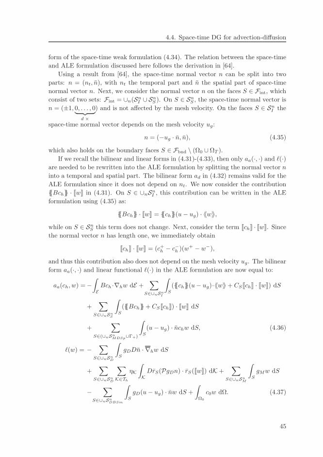
4.4. Space-time DG for advection-diffusion
form of the space-time weak formulation (4.34). The relation between the space-time
and ALE formulation discussed here follows the derivation in [64].
Using a result from [64], the space-time normal vector n can be split into two
parts: n = (nt, n), with nt the temporal part and n the spatial part of space-time
normal vector n. Next, we consider the normal vector n on the faces S ∈ Fint, which
consist of two sets: Fint = ∪n(SnI ∪ Sn
S ). On S ∈ SnS , the space-time normal vector is
n = (±1, 0, . . . , 0︸ ︷︷ ︸
d ×
) and is not affected by the mesh velocity. On the faces S ∈ SnI the
space-time normal vector depends on the mesh velocity ug:
n = (−ug · n, n), (4.35)
which also holds on the boundary faces S ∈ Fbnd \ (Ω0 ∪ΩT ).
If we recall the bilinear and linear forms in (4.31)-(4.33), then only aa(·, ·) and ℓ(·)are needed to be rewritten into the ALE formulation by splitting the normal vector n
into a temporal and spatial part. The bilinear form ad in (4.32) remains valid for the
ALE formulation since it does not depend on nt. We now consider the contribution
Bch · [[w]] in (4.31). On S ∈ ∪nSnI , this contribution can be written in the ALE
formulation using (4.35) as:
Bch · [[w]] = ch(u− ug) · 〈〈w〉〉,
while on S ∈ SnS this term does not change. Next, consider the term [[ch]] · [[w]]. Since
the normal vector n has length one, we immediately obtain
[[ch]] · [[w]] = (c+h − c−h )(w+ − w−),
and thus this contribution also does not depend on the mesh velocity ug. The bilinear
form aa(·, ·) and linear functional ℓ(·) in the ALE formulation are now equal to:
aa(ch, w) =−∫
EBch ·∇hw dE +
∑
S∈∪nSnI
∫
S
(ch(u− ug)·〈〈w〉〉+ CS [[ch]] · [[w]]) dS
+∑
S∈∪nSnS
∫
S
(Bch+ CS [[ch]]) · [[w]] dS
+∑
S∈(∪nSnMDSp
∪Γ+)
∫
S
(u − ug) · nchw dS, (4.36)
ℓ(w) = −∑
S∈∪nSnD
∫
S
gDDn · ∇hw dS
+∑
S∈∪nSnD
∑
K∈Th
ηK
∫
KDrS(PgDn) · rS([[w]]) dK +
∑
S∈∪nSnM
∫
S
gMw dS
−∑
S∈∪nSnDBSm
∫
S
gD(u− ug) · nw dS +
∫
Ω0
c0w dΩ. (4.37)
45
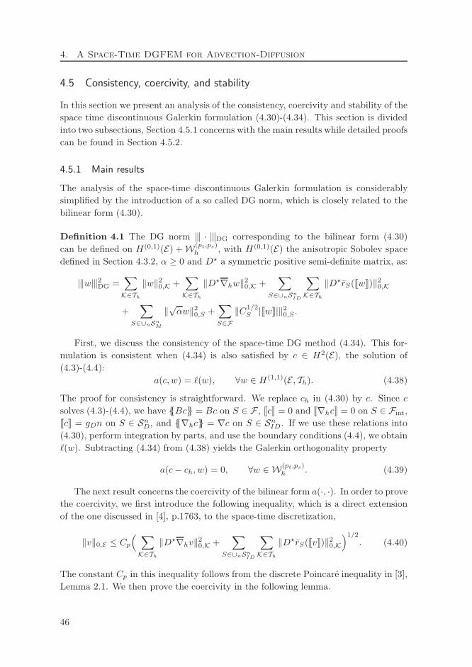
4. A Space-Time DGFEM for Advection-Diffusion
4.5 Consistency, coercivity, and stability
In this section we present an analysis of the consistency, coercivity and stability of the
space time discontinuous Galerkin formulation (4.30)-(4.34). This section is divided
into two subsections, Section 4.5.1 concerns with the main results while detailed proofs
can be found in Section 4.5.2.
4.5.1 Main results
The analysis of the space-time discontinuous Galerkin formulation is considerably
simplified by the introduction of a so called DG norm, which is closely related to the
bilinear form (4.30).
Definition 4.1 The DG norm |‖ · ‖|DG corresponding to the bilinear form (4.30)
can be defined on H(0,1)(E) +W(pt,ps)h , with H(0,1)(E) the anisotropic Sobolev space
defined in Section 4.3.2, α ≥ 0 and D⋆ a symmetric positive semi-definite matrix, as:
|‖w‖|2DG =∑
K∈Th
‖w‖20,K +∑
K∈Th
‖D⋆∇hw‖20,K +∑
S∈∪nSnID
∑
K∈Th
‖D⋆rS([[w]])‖20,K
+∑
S∈∪nSnM
‖√αw‖20,S +∑
S∈F‖C1/2
S |[[w]]|‖20,S .
First, we discuss the consistency of the space-time DG method (4.34). This for-
mulation is consistent when (4.34) is also satisfied by c ∈ H2(E), the solution of
(4.3)-(4.4):
a(c, w) = ℓ(w), ∀w ∈ H(1,1)(E , Th). (4.38)
The proof for consistency is straightforward. We replace ch in (4.30) by c. Since c
solves (4.3)-(4.4), we have Bc = Bc on S ∈ F , [[c]] = 0 and [[∇hc]] = 0 on S ∈ Fint,
[[c]] = gDn on S ∈ SnD, and ∇hc = ∇c on S ∈ Sn
ID. If we use these relations into
(4.30), perform integration by parts, and use the boundary conditions (4.4), we obtain
ℓ(w). Subtracting (4.34) from (4.38) yields the Galerkin orthogonality property
a(c− ch, w) = 0, ∀w ∈ W(pt,ps)h . (4.39)
The next result concerns the coercivity of the bilinear form a(·, ·). In order to prove
the coercivity, we first introduce the following inequality, which is a direct extension
of the one discussed in [4], p.1763, to the space-time discretization,
‖v‖0,E ≤ Cp
( ∑
K∈Th
‖D⋆∇hv‖20,K +∑
S∈∪nSnID
∑
K∈Th
‖D⋆rS([[v]])‖20,K
)1/2
. (4.40)
The constant Cp in this inequality follows from the discrete Poincare inequality in [3],
Lemma 2.1. We then prove the coercivity in the following lemma.
46
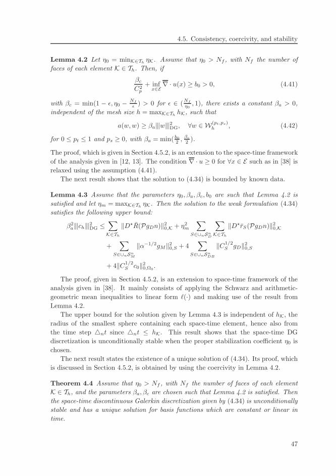
4.5. Consistency, coercivity, and stability
Lemma 4.2 Let η0 = minK∈ThηK. Assume that η0 > Nf , with Nf the number of
faces of each element K ∈ Th. Then, if
βc
C2p
+ infx∈E∇ · u(x) ≥ b0 > 0, (4.41)
with βc = min(1 − ǫ, η0 − Nf
ǫ ) > 0 for ǫ ∈ (Nf
η0, 1), there exists a constant βa > 0,
independent of the mesh size h = maxK∈ThhK, such that
a(w,w) ≥ βa|‖w‖|2DG, ∀w ∈ W(pt,ps)h , (4.42)
for 0 ≤ pt ≤ 1 and ps ≥ 0, with βa = min( b02 ,
βc
2 ).
The proof, which is given in Section 4.5.2, is an extension to the space-time framework
of the analysis given in [12, 13]. The condition ∇ · u ≥ 0 for ∀x ∈ E such as in [38] is
relaxed using the assumption (4.41).
The next result shows that the solution to (4.34) is bounded by known data.
Lemma 4.3 Assume that the parameters η0, βa, βc, b0 are such that Lemma 4.2 is
satisfied and let ηm = maxK∈ThηK. Then the solution to the weak formulation (4.34)
satisfies the following upper bound:
β2a|‖ch‖|2DG ≤
∑
K∈Th
‖D⋆R(PgDn)‖20,K + η2m
∑
S∈∪nSnD
∑
K∈Th
‖D⋆rS(PgDn)‖20,K
+∑
S∈∪nSnM
‖α−1/2gM‖20,S + 4∑
S∈∪nSnDB
‖C1/2S gD‖20,S
+ 4‖C1/2S c0‖20,Ω0
.
The proof, given in Section 4.5.2, is an extension to space-time framework of the
analysis given in [38]. It mainly consists of applying the Schwarz and arithmetic-
geometric mean inequalities to linear form ℓ(·) and making use of the result from
Lemma 4.2.
The upper bound for the solution given by Lemma 4.3 is independent of hK, the
radius of the smallest sphere containing each space-time element, hence also from
the time step nt since nt ≤ hK. This result shows that the space-time DG
discretization is unconditionally stable when the proper stabilization coefficient η0 is
chosen.
The next result states the existence of a unique solution of (4.34). Its proof, which
is discussed in Section 4.5.2, is obtained by using the coercivity in Lemma 4.2.
Theorem 4.4 Assume that η0 > Nf , with Nf the number of faces of each element
K ∈ Th, and the parameters βa, βc are chosen such that Lemma 4.2 is satisfied. Then
the space-time discontinuous Galerkin discretization given by (4.34) is unconditionally
stable and has a unique solution for basis functions which are constant or linear in
time.
47
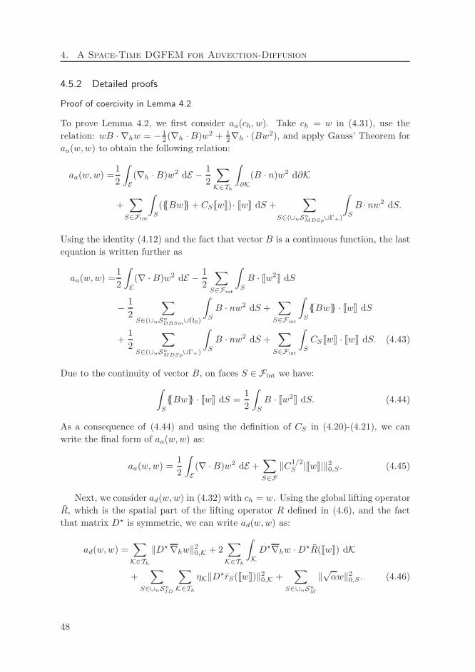
4. A Space-Time DGFEM for Advection-Diffusion
4.5.2 Detailed proofs
Proof of coercivity in Lemma 4.2
To prove Lemma 4.2, we first consider aa(ch, w). Take ch = w in (4.31), use the
relation: wB · ∇hw = − 12 (∇h · B)w2 + 1
2∇h · (Bw2), and apply Gauss’ Theorem for
aa(w,w) to obtain the following relation:
aa(w,w) =1
2
∫
E(∇h ·B)w2 dE − 1
2
∑
K∈Th
∫
∂K(B · n)w2 d∂K
+∑
S∈Fint
∫
S
(Bw+ CS [[w]])· [[w]] dS +∑
S∈(∪nSnMDSp
∪Γ+)
∫
S
B · nw2 dS.
Using the identity (4.12) and the fact that vector B is a continuous function, the last
equation is written further as
aa(w,w) =1
2
∫
E(∇ · B)w2 dE − 1
2
∑
S∈Fint
∫
S
B · [[w2]] dS
− 1
2
∑
S∈(∪nSnDBSm
∪Ω0)
∫
S
B · nw2 dS +∑
S∈Fint
∫
S
Bw · [[w]] dS
+1
2
∑
S∈(∪nSnMDSp
∪Γ+)
∫
S
B · nw2 dS +∑
S∈Fint
∫
S
CS [[w]] · [[w]] dS. (4.43)
Due to the continuity of vector B, on faces S ∈ Fint we have:
∫
S
Bw · [[w]] dS =1
2
∫
S
B · [[w2]] dS. (4.44)
As a consequence of (4.44) and using the definition of CS in (4.20)-(4.21), we can
write the final form of aa(w,w) as:
aa(w,w) =1
2
∫
E(∇ · B)w2 dE +
∑
S∈F‖C1/2
S |[[w]]|‖20,S . (4.45)
Next, we consider ad(w,w) in (4.32) with ch = w. Using the global lifting operator
R, which is the spatial part of the lifting operator R defined in (4.6), and the fact
that matrix D⋆ is symmetric, we can write ad(w,w) as:
ad(w,w) =∑
K∈Th
‖D⋆∇hw‖20,K + 2∑
K∈Th
∫
KD⋆∇hw ·D⋆R([[w]]) dK
+∑
S∈∪nSnID
∑
K∈Th
ηK‖D⋆rS([[w]])‖20,K +∑
S∈∪nSnM
‖√αw‖20,S . (4.46)
48
4.5. Consistency, coercivity, and stability
Using the Schwarz and arithmetic-geometric mean inequalities we obtain
2
∫
KD⋆∇hw ·D⋆R([[w]]) dK ≥ −ǫ‖D⋆∇hw‖20,K −
1
ǫ‖D⋆R([[w]])‖20,K, (4.47a)
with ǫ > 0. As a consequence of (4.6) and the fact that the local lifting operator rSis only non-zero in the elements connected to the face S, we also have
‖D⋆R([[w]])‖20,K ≤ Nf
∑
S∈∪nSnID
‖D⋆rS([[w]])‖20,K, (4.47b)
with Nf the number of faces of each element K ∈ Th. Introducing (4.47a)-(4.47b)
into (4.46) and combining with (4.45), we deduce
a(w,w) ≥ 1
2
∫
E(∇ · u)w2 dE +
(1− ǫ
) ∑
K∈Th
‖D⋆∇hw‖20,K
+(η0 −
Nf
ǫ
) ∑
S∈∪nSnID
∑
K∈Th
‖D⋆rS([[w]])‖20,K
+∑
S∈∪nSnM
‖√αw‖20,S +∑
S∈F‖C1/2
S |[[w]]|‖20,S , (4.48)
with η0 defined as η0 = minK∈ThηK. If we take η0 > Nf and ǫ ∈ (
Nf
η0, 1), and choosing
βc = min(1− ǫ, η0 − Nf
ǫ ) > 0, we obtain
a(w,w) ≥1
2
∫
E(∇·u)w2 dE + βc
∑
K∈Th
‖D⋆∇hw‖20,K + βc
∑
S∈∪nSnID
∑
K∈Th
‖D⋆rS([[w]])‖20,K
+∑
S∈∪nSnM
‖√αw‖20,S +∑
S∈F‖C1/2
S |[[w]]|‖20,S . (4.49)
Making use inequality (4.40) into (4.49) and assuming the existence of b0 > 0 that
satisfies (4.41), we then obtain:
a(w,w) ≥ b02‖w‖20,E+
βc
2
∑
K∈Th
‖D⋆∇hw‖20,K+βc
2
∑
S∈∪nSnID
∑
K∈Th
‖D⋆rS([[w]])‖20,K
+∑
S∈∪nSnM
‖√αw‖20,S +∑
S∈F‖C1/2
S |[[w]]|‖20,S . (4.50)
Since βc/2 is always less than one, choosing βa = min( b02 ,
βc
2 ) completes the proof of
the coercivity.
Proof of boundedness in Lemma 4.3
To prove Lemma 4.3, we take w = ch in (4.34), which results in the relation:
a(ch, ch) = ℓ(ch). (4.51)
49
4. A Space-Time DGFEM for Advection-Diffusion
Using the lifting operator R in (4.8), the symmetry of matrix D, and the definition
of CS on S ∈ Fbnd given by (4.21), the linear functional ℓ(ch) can be written as:
ℓ(ch) =∑
K∈Th
∫
KD⋆R(PgDn) ·D⋆∇hch dK
+∑
S∈∪nSnD
∑
K∈Th
ηK
∫
KD⋆rS(PgDn) ·D⋆rS([[ch]]) dK +
∑
S∈∪nSnM
∫
S
gMch dS
+ 2∑
S∈∪nSnDBSm
∫
S
CSgDch dS + 2
∫
Ω0
CSc0ch dΩ. (4.52)
Applying the Schwarz and arithmetic-geometric mean inequalities on each term in
(4.52) and combining this result with (4.51) and Lemma 4.2 using w = ch, we obtain
the inequality
βa‖ch‖20,E +(βa−
ǫ12
) ∑
K∈Th
‖D⋆∇hch‖20,K+(βa−
ηmǫ22
) ∑
S∈∪nSnID
∑
K∈Th
‖D⋆rS([[ch]])‖20,K
+(βa−
ǫ32
) ∑
S∈∪nSnM
‖√αch‖20,S +(βa−ǫ4
) ∑
S∈F‖C1/2
S |[[ch]]|‖20,S
≤ 1
2ǫ1
∑
K∈Th
‖D⋆R(PgDn)‖20,K +ηm
2ǫ2
∑
S∈∪nSnD
∑
K∈Th
‖D⋆rS(PgDn)‖20,K
+1
2ǫ3
∑
S∈∪nSnM
‖α−1/2gM‖20,S+1
ǫ4
∑
S∈∪nSnDBSm
‖C1/2S gD‖20,S +
1
ǫ4‖C1/2
S c0‖20,Ω0, (4.53)
with ǫ1, . . . , ǫ4 > 0 and ηm = maxK∈ThηK. Next, we substitute the following coef-
ficients: ǫ1 = βa, ǫ2 = βa
ηm, ǫ3 = βa, and ǫ4 = βa
2 into (4.53) and multiply the result
with 2βa to complete the proof.
Proof of the uniqueness in Theorem 4.4
To prove the uniqueness of the solution it is sufficient to show that the following
homogeneous equation:
Find a ch ∈ W(pt,ps)h such that:
a(ch, w) = 0, ∀w ∈ W(pt,ps)h , with ch(0, x) = 0, (4.54)
has only the trivial solution ch = 0 for all t > 0.
We proceed as follows. Assume that ch is a solution of (4.54) and take w = ch in
(4.30). Then we rewrite (4.42) as:
a(ch, ch) ≥βa
Nt−1∑
n=0
(∑
K∈T nh
‖ch‖20,K +∑
K∈T nh
‖D⋆∇hch‖20,K +∑
S∈SnID
∑
K∈T nh
‖D⋆rS([[ch]])‖20,K
+∑
S∈SnM
‖√αch‖20,S +∑
S∈Fn
‖C1/2S |[[ch]]|‖20,S
)
.
50
4.6. Error estimates and hp-convergence
Consider now the space-time slab for n = 0. The coercivity condition, in combination
with the initial condition c+h = 0 at t = 0 and (4.54), implies that ch = 0 in the
first space-time slab when constant or linear polynomials in time are used. We can
continue this argument to the other space-time slabs and obtain that ch = 0 is the
only solution possible for the homogeneous equation. Hence the DG algorithm has a
unique solution ch for constant or linear basis functions in time. The unconditional
stability of the DG algorithm is a direct consequence of Lemma 4.3.
4.6 Error estimates and hp-convergence
First, let us define the projection P : L2(E)→W(pt,ps)h as:
∑
K∈Th
(Pc, w)K =∑
K∈Th
(c, w)K, ∀w ∈ W(pt,ps)h , (4.55)
which can be used to decompose the global error c− ch as:
c− ch = (c− Pc) + (Pc− ch) ≡ ρ+ θ, (4.56)
with ρ the interpolation error and θ the discretization error. In the next section we
discuss the upper bounds for the interpolation error ρ.
4.6.1 Bounds for the interpolation error
In this section we present the upper bounds for the interpolation error ρ = c − Pc.These estimates are an extension of the bounds for the interpolation error derived
in [31] to general dimensions. We restrict the derivations for a separate polynomial
degree pt,K in time and a polynomial degree ps,K in each spatial variable.
Lemma 4.5 Assume that K is a space-time element in Rd+1 constructed via two
mappings QK, FK, with FK : K → K and QK : K → K. Assume also that hi,K, i =
1, . . . , d is the edge length of K in the xi direction, and nt the edge length in the
x0 direction (see illustration in Fig. 4.2 for d = 2). Let c|K ∈ H(kt,K+1,ks,K+1)(K),
with kt,K, ks,K ≥ 0. Let P denote the L2 projection of c onto the finite element space
W(pt,ps)h . Then the projection error ρ = c−Pc in K and its trace at the boundary ∂K
obey the error bounds:
‖ρ‖20,K ≤CZK, (4.57)
‖∇hρ‖20,K ≤CNK, (4.58)
‖ρ‖20,∂K ≤C(AK +BK), (4.59)
51
4. A Space-Time DGFEM for Advection-Diffusion
where
ZK =
d∑
i=1
(hi,Kps,K
)2sK
‖∂sK
i c‖20,K +
(nt
pt,K
)2s0,K
‖∂s0,K
0 c‖20,K,
NK =
d∑
i=1
h2tKi,K
p2tK−1s,K
‖∂tK+1i c‖2
0,K +
d∑
i=1
∑
j 6=i
h2tK+2j,K
p2tKs,K‖∂tK+1
j ∂ic‖20,K
+
d∑
i=1
(nt)2t0,K+2
p2t0,K
t,K‖∂t0,K+1
0 ∂ic‖20,K,
AK =
d∑
i=1
(hi,Kps,K
)2tK+1
‖∂tK+1i c‖2
0,K +
d∑
i=1
∑
j 6=i
1
hi,K
(hj,Kps,K
)2sK
‖∂sK
j c‖20,K
+
d∑
i=1
∑
j 6=i
hi,Kps,K
(hj,Kps,K
)2qK‖∂qK
j ∂ic‖20,K,
BK =
d∑
i=1
1
hi,K
(nt
pt,K
)2s0,K
‖∂s0,K
0 c‖20,K +
d∑
i=1
hi,Kps,K
(nt
pt,K
)2q0,K
‖∂q0,K
0 ∂ic‖20,K
+(nt
pt,K
)2t0,K+1
‖∂t0,K+10 c‖2
0,K +1
nt
d∑
i=1
(hi,Kps,K
)2sK
‖∂sK
i c‖20,K
+nt
pt,K
d∑
i=1
(hi,Kps,K
)2qK‖∂qK
i ∂0c‖20,K,
with pt,K and ps,K the local polynomial degree in time and space, respectively, on
element K, 0 < s0,K ≤ min(pt,K + 1, kt,K + 1), 0 < sK ≤ min(ps,K + 1, ks,K + 1), 0 <
q0,K ≤ min(pt,K + 1, kt,K), 0 < qK ≤ min(ps,K + 1, ks,K), 0 < t0,K ≤ min(pt,K, kt,K),
and 0 < tK ≤ min(ps,K, ks,K). The constant C has a positive value that depends only
on the spatial dimension d and the mapping QK.
Remark 4.6 In particular, when c is sufficiently smooth and the spatial shape of
element K is regular: hK = hi,K, i = 1, . . . , d, we obtain the following leading terms
for each estimate given in Lemma 4.5:
‖ρ‖20,K ≤ C(h
2ps,K+2Kp2ps,K+2s,K
+nt
2pt,K+2
p2pt,K+2t,K
)
|c|2pt,K+1,ps,K+1,K,
‖∇hρ‖20,K ≤ C( h
2ps,K
Kp2ps,K−1s,K
+nt
2pt,K+2
p2pt,K
t,K
)
|c|2pt,K+1,ps,K+1,K,
‖ρ‖20,∂K ≤ C(h
2ps,K+1Kp2ps,K+1s,K
+nt
2pt,K+1
p2pt,K+1t,K
)
|c|2pt,K+1,ps,K+1,K.
52
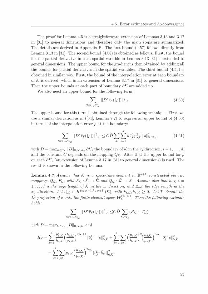
4.6. Error estimates and hp-convergence
The proof for Lemma 4.5 is a straightforward extension of Lemmas 3.13 and 3.17
in [31] to general dimensions and therefore only the main steps are summarized.
The details are derived in Appendix B. The first bound (4.57) follows directly from
Lemma 3.13 in [31]. The second bound (4.58) is obtained as follows. First, the bound
for the partial derivative in each spatial variable in Lemma 3.13 [31] is extended to
general dimensions. The upper bound for the gradient is then obtained by adding all
the bounds for partial derivatives in the spatial variables. The third bound (4.59) is
obtained in similar way. First, the bound of the interpolation error at each boundary
of K is derived, which is an extension of Lemma 3.17 in [31] to general dimensions.
Then the upper bounds at each part of boundary ∂K are added up.
We also need an upper bound for the following term:∑
S∈∪nSnID
‖D⋆rS([[ρ]])‖20,E . (4.60)
The upper bound for this term is obtained through the following technique. First, we
use a similar derivation as in ([54], Lemma 7.2) to express an upper bound of (4.60)
in terms of the interpolation error ρ at the boundary:
∑
S∈∪nSnID
‖D⋆rS([[ρ]])‖20,E ≤ CD∑
K
d∑
i=1
h−1i,Kp
2s,K‖ρ‖20,∂Ki
, (4.61)
with D = maxK∈Th‖D‖0,∞,K, ∂Ki the boundary of K in the xi direction, i = 1, . . . , d,
and the constant C depends on the mapping QK. After that the upper bound for ρ
on each ∂Ki (an extension of Lemma 3.17 in [31] to general dimensions) is used. The
result is shown in the following Lemma.
Lemma 4.7 Assume that K is a space-time element in Rd+1 constructed via two
mappings QK, FK, with FK : K → K and QK : K → K. Assume also that hi,K, i =
1, . . . , d is the edge length of K in the xi direction, and nt the edge length in the
x0 direction. Let c|K ∈ H(kt,K+1,ks,K+1)(K), with kt,K, ks,K ≥ 0. Let P denote the
L2 projection of c onto the finite element space W(pt,ps)h . Then the following estimate
holds:∑
S∈∪nSnID
‖D⋆rS([[ρ]])‖20,E ≤CD∑
K∈Th
(RK + TK),
with D = maxK∈Th‖D‖0,∞,K and
RK =d∑
i=1
p2s,Khi,K
(hi,Kps,K
)2tK+1
‖∂tK+1i c‖2
0,K +d∑
i=1
∑
j 6=i
(ps,Khi,K
)2(hj,Kps,K
)2sK
‖∂sK
j c‖20,K
+d∑
i=1
∑
j 6=i
ps,K(hj,Kps,K
)2qK‖∂qK
j ∂ic‖20,K,
53
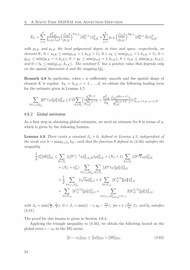
4. A Space-Time DGFEM for Advection-Diffusion
TK =
d∑
i=1
p2s,K
hi,Knt
(nt
pt,K
)2s0,K
‖∂s0,K
0 c‖20,K +
d∑
i=1
ps,K(nt
pt,K
)2q0,K
‖∂q0,K
0 ∂ic‖20,K,
with pt,K and ps,K the local polynomial degree in time and space, respectively, on
element K, 0 < s0,K ≤ min(pt,K + 1, kt,K + 1), 0 < sK ≤ min(ps,K + 1, ks,K + 1), 0 <
q0,K ≤ min(pt,K + 1, kt,K), 0 < qK ≤ min(ps,K + 1, ks,K), 0 < t0,K ≤ min(pt,K, kt,K),
and 0 < tK ≤ min(ps,K, ks,K). The constant C has a positive value that depends only
on the spatial dimension d and the mapping QK.
Remark 4.8 In particular, when c is sufficiently smooth and the spatial shape of
element K is regular: hK = hi,K, i = 1, . . . , d, we obtain the following leading term
for the estimate given in Lemma 4.7:
∑
S∈∪nSnID
‖D⋆rS([[ρ]])‖20,E≤CD∑
K∈Th
( h2ps,K
Kp2ps,K−1s,K
+p2
s,KhK
nt2pt,K+1
p2pt,K+2t,K
)
|c|2pt,K+1,ps,K+1,K.
4.6.2 Global estimates
As a first step in obtaining global estimates, we need an estimate for θ in terms of ρ,
which is given by the following Lemma.
Lemma 4.9 There exists a constant βa > 0, defined in Lemma 4.2, independent of
the mesh size h = maxK∈ThhK, such that the function θ defined in (4.56) satisfies the
inequality
1
4β2
a|‖θ‖|2DG ≤∑
K∈Th
‖(D⋆)−1u‖20,∞,K‖ρ‖20,K + (Nf + 1)∑
K∈Th
‖D⋆∇hρ‖20,K
+ (Nf + η2m)
∑
S∈∪nSnID
∑
K∈Th
‖D⋆rS([[ρ]])‖20,K
+1
2
∑
S∈∪nSnM
‖√αρ‖20,S + 2∑
S∈Fint
‖C1/2S ρ‖20,S
+∑
S∈Fint
‖C1/2S |[[ρ]]|‖20,S +
∑
S∈(∪nSnMDSp
∪Γ+)
2‖C1/2S |[[ρ]]|‖20,S ,
with βa = min( b02 ,
βc
2 ), 0 < βc = min(1− ǫ, η0 − Nf
ǫ ), for ǫ ∈ (Nf
η0, 1), and b0 satisfies
(4.41).
The proof for this lemma is given in Section 4.6.4.
Applying the triangle inequality to (4.56), we obtain the following bound on the
global error c− ch in the DG norm:
|‖c− ch‖|DG ≤ |‖ρ‖|DG + |‖θ‖|DG. (4.62)
54
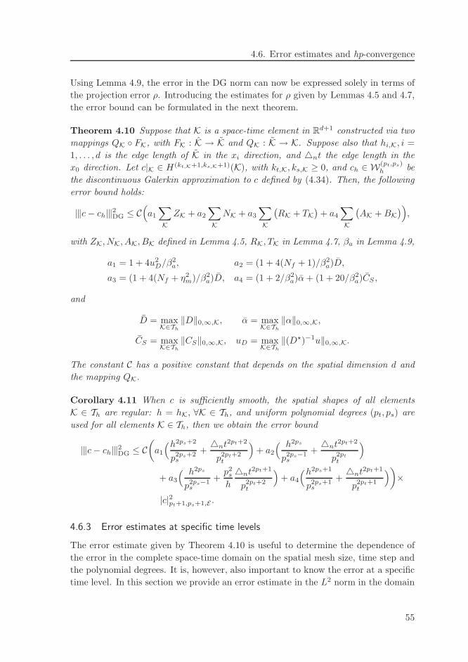
4.6. Error estimates and hp-convergence
Using Lemma 4.9, the error in the DG norm can now be expressed solely in terms of
the projection error ρ. Introducing the estimates for ρ given by Lemmas 4.5 and 4.7,
the error bound can be formulated in the next theorem.
Theorem 4.10 Suppose that K is a space-time element in Rd+1 constructed via two
mappings QK FK, with FK : K → K and QK : K → K. Suppose also that hi,K, i =
1, . . . , d is the edge length of K in the xi direction, and nt the edge length in the
x0 direction. Let c|K ∈ H(kt,K+1,ks,K+1)(K), with kt,K, ks,K ≥ 0, and ch ∈ W(pt,ps)h be
the discontinuous Galerkin approximation to c defined by (4.34). Then, the following
error bound holds:
|‖c− ch‖|2DG ≤ C(
a1
∑
KZK + a2
∑
KNK + a3
∑
K
(RK + TK
)+ a4
∑
K
(AK +BK
))
,
with ZK, NK, AK, BK defined in Lemma 4.5, RK, TK in Lemma 4.7, βa in Lemma 4.9,
a1 = 1 + 4u2D/β
2a, a2 = (1 + 4(Nf + 1)/β2
a)D,
a3 = (1 + 4(Nf + η2m)/β2
a)D, a4 = (1 + 2/β2a)α+ (1 + 20/β2
a)CS ,
and
D = maxK∈Th
‖D‖0,∞,K, α = maxK∈Th
‖α‖0,∞,K,
CS = maxK∈Th
‖CS‖0,∞,K, uD = maxK∈Th
‖(D⋆)−1u‖0,∞,K.
The constant C has a positive constant that depends on the spatial dimension d and
the mapping QK.
Corollary 4.11 When c is sufficiently smooth, the spatial shapes of all elements
K ∈ Th are regular: h = hK, ∀K ∈ Th, and uniform polynomial degrees (pt, ps) are
used for all elements K ∈ Th, then we obtain the error bound
|‖c− ch‖|2DG ≤ C(
a1
(h2ps+2
p2ps+2s
+nt
2pt+2
p2pt+2t
)
+ a2
( h2ps
p2ps−1s
+nt
2pt+2
p2pt
t
)
+ a3
( h2ps
p2ps−1s
+p2
s
h
nt2pt+1
p2pt+2t
)
+ a4
(h2ps+1
p2ps+1s
+nt
2pt+1
p2pt+1t
))
×
|c|2pt+1,ps+1,E .
4.6.3 Error estimates at specific time levels
The error estimate given by Theorem 4.10 is useful to determine the dependence of
the error in the complete space-time domain on the spatial mesh size, time step and
the polynomial degrees. It is, however, also important to know the error at a specific
time level. In this section we provide an error estimate in the L2 norm in the domain
55
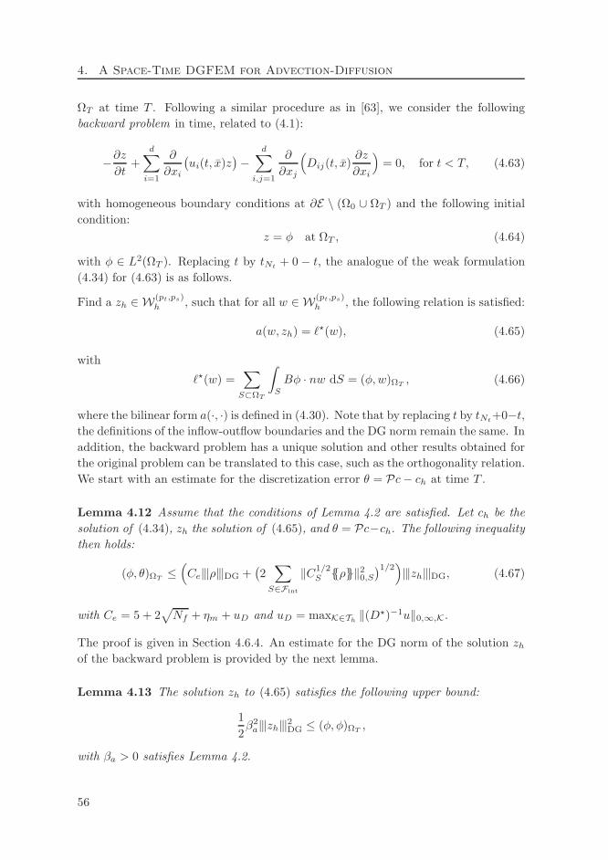
4. A Space-Time DGFEM for Advection-Diffusion
ΩT at time T . Following a similar procedure as in [63], we consider the following
backward problem in time, related to (4.1):
−∂z∂t
+
d∑
i=1
∂
∂xi
(ui(t, x)z
)−
d∑
i,j=1
∂
∂xj
(
Dij(t, x)∂z
∂xi
)
= 0, for t < T, (4.63)
with homogeneous boundary conditions at ∂E \ (Ω0 ∪ ΩT ) and the following initial
condition:
z = φ at ΩT , (4.64)
with φ ∈ L2(ΩT ). Replacing t by tNt+ 0 − t, the analogue of the weak formulation
(4.34) for (4.63) is as follows.
Find a zh ∈ W(pt,ps)h , such that for all w ∈ W(pt,ps)
h , the following relation is satisfied:
a(w, zh) = ℓ⋆(w), (4.65)
with
ℓ⋆(w) =∑
S⊂ΩT
∫
S
Bφ · nw dS = (φ,w)ΩT, (4.66)
where the bilinear form a(·, ·) is defined in (4.30). Note that by replacing t by tNt+0−t,
the definitions of the inflow-outflow boundaries and the DG norm remain the same. In
addition, the backward problem has a unique solution and other results obtained for
the original problem can be translated to this case, such as the orthogonality relation.
We start with an estimate for the discretization error θ = Pc− ch at time T .
Lemma 4.12 Assume that the conditions of Lemma 4.2 are satisfied. Let ch be the
solution of (4.34), zh the solution of (4.65), and θ = Pc−ch. The following inequality
then holds:
(φ, θ)ΩT≤
(
Ce|‖ρ‖|DG +(2
∑
S∈Fint
‖C1/2S ρ‖20,S
)1/2)
|‖zh‖|DG, (4.67)
with Ce = 5 + 2√Nf + ηm + uD and uD = maxK∈Th
‖(D⋆)−1u‖0,∞,K.
The proof is given in Section 4.6.4. An estimate for the DG norm of the solution zh
of the backward problem is provided by the next lemma.
Lemma 4.13 The solution zh to (4.65) satisfies the following upper bound:
1
2β2
a|‖zh‖|2DG ≤ (φ, φ)ΩT,
with βa > 0 satisfies Lemma 4.2.
56
4.6. Error estimates and hp-convergence
The proof is given in Section 4.6.4. Using Lemma 4.13, the estimate given by (4.67)
can further be written as
(φ, θ)ΩT≤√
2
βa
(
Ce|‖ρ‖|DG +(2
∑
S∈Fint
‖C1/2S ρ‖20,S
)1/2)
‖φ‖0,ΩT.
After using the relation
‖θ‖0,ΩT= sup
06=φ∈L2(ΩT )
(φ, θ)ΩT
‖φ‖0,ΩT
,
we then have
‖θ‖0,ΩT≤√
2
βa
(
Ce|‖ρ‖|DG +(2
∑
S∈Fint
‖C1/2S ρ‖20,S
)1/2)
. (4.68)
Using the hp-estimates for ρ in Lemma 4.5, we obtain the following bound.
Theorem 4.14 Suppose that K is a space-time element in Rd+1 constructed via two
mappings QK FK, with FK : K → K and QK : K → K. Suppose also that hi,K, i =
1, . . . , d is the edge length of K in the xi direction, and nt the edge length in the
x0 direction. Let c|K ∈ H(kt,K+1,ks,K+1)(K), with kt,K, ks,K ≥ 0 and ch ∈ W(pt,ps)h be
the discontinuous Galerkin approximation to c defined by (4.34). Then the following
error bound holds:
‖c− ch‖20,ΩT≤ C
(∑
K
(
b1ZK + b2(NK +RK + TK
)+ (b3 + b4)
(AK +BK
)))
,
with ZK, NK, AK, BK defined in Lemma 4.5, RK, TK in Lemma 4.7,
b1 = 2C2e/β
2a, b2 =
(2C2
e/β2a
)D,
b3 =(2C2
e/β2a
)α, b4 =
(2C2
e/β2a + 4/β2
a + 1)CS ,
the coefficients D, α, CS given in Theorem 4.10, Ce in Lemma 4.12, and βa satisfies
Lemma 4.2. The constant C has a positive value that depends only on the spatial
dimension d and the mapping QK.
The proof of this theorem is immediate using (4.68) and Lemma 4.5.
Corollary 4.15 When c is sufficiently smooth, the spatial shapes of all elements
K ∈ Th are regular: h = hK, ∀K ∈ Th, and uniform polynomial degrees (pt, ps) are
used for all elements K ∈ Th, then we obtain the error bound
‖c− ch‖20,ΩT≤C
(
b1
(h2ps+2
p2ps+2s
+nt
2pt+2
p2pt+2t
)
+b2
(
2h2ps
p2ps−1s
+nt
2pt+2
p2pt
t
+p2
s
h
nt2pt+2
p2pt
t
)
+(b3 + b4)(h2ps+1
p2ps+1s
+nt
2pt+1
p2pt+1t
))
|c|2pt+1,ps+1,E .
57
4. A Space-Time DGFEM for Advection-Diffusion
4.6.4 Proofs
Proof of the upper bound for the discretization error θ in Lemma 4.9
The proof of Lemma 4.9 starts with the orthogonality relation (4.39) and the decom-
position of the error (4.56), which imply that
a(θ + ρ, w) = 0, ∀w ∈ W(pt,ps)h . (4.69)
Taking w = θ, we obtain a(θ, θ) = −a(ρ, θ). We continue with the derivation of
an estimate for |a(ρ, θ)|. First, we consider the bilinear form aa(ρ, θ). Since θ ∈W(pt,ps)
h , which is a polynomial function, we have ∂θ∂t ∈ W
(pt,ps)h and we can use the
L2 orthogonality relation for the projection P , given by (4.55), to obtain:
aa(ρ, θ) =−∑
K∈Th
∫
K(D⋆)−1uρ ·D⋆∇hθ dK +
∑
S∈Fint
∫
S
Bρ · [[θ]] dS
+∑
S∈Fint
∫
S
CS [[ρ]] · [[θ]] dS +∑
S∈(∪nSnMDSp
∪Γ+)
∫
S
B · nρθ dS. (4.70)
Using the same argument as in [13], that is by using (4.20) and the continuity property
of B, we have: |Bρ · n| = |B · n||ρ| = 2CS |ρ|. Then, by using the Schwarz
inequality together with the arithmetic-geometric mean inequality in the form: pq ≤p2
β + βq2
4 , we have the following estimate:
|aa(ρ, θ)| ≤ 1
β
∑
K∈Th
‖(D⋆)−1u‖20,∞,K‖ρ‖20,K +2
β
∑
S∈Fint
‖C1/2S ρ‖20,S
+1
β
∑
S∈Fint
‖C1/2S |[[ρ]]|‖20,S +
2
β
∑
S∈(∪nSnMDSp
∪Γ+)
‖C1/2S |[[ρ]]|‖20,S
+1
4β
∑
K∈Th
‖D⋆∇hθ‖20,K +3
4β
∑
S∈Fint
‖C1/2S |[[θ]]|‖20,S
+1
2β
∑
S∈(∪nSnMDSp
∪Γ+)
‖C1/2S |[[θ]]|‖20,S . (4.71)
Next, we consider the bilinear form ad(ρ, θ). Using the lifting operator R, the
bilinear form can be written as:
ad(ρ, θ) =∑
K∈Th
∫
KD∇hρ·∇hθ dK+
∑
K∈Th
∫
KR([[ρ]])·D∇hθ dK +
∑
K∈Th
∫
KD∇hρ·R([[θ]]) dK
+∑
S∈∪nSnID
∑
K∈Th
ηK
∫
KDrS([[ρ]])·rS([[θ]]) dK +
∑
S∈∪nSnM
∫
S
αρθ dS. (4.72)
58
4.6. Error estimates and hp-convergence
Applying the Schwarz’ inequality, inequality (4.47b) and arithmetic-geometric mean
inequality yields:
|ad(ρ, θ)| ≤Nf + 1
β
∑
K∈Th
‖D⋆∇hρ‖20,K +Nf + η2
m
β
∑
S∈∪nSnID
∑
K∈Th
‖D⋆rS([[ρ]])‖20,K
+1
2β
∑
S∈∪nSnM
‖√αρ‖20,S +β
2
∑
K∈Th
‖D⋆∇hθ‖20,K
+β
2
∑
S∈∪nSnID
∑
K∈Th
‖D⋆rS([[θ]])‖2L2(K) +β
2
∑
S∈∪nSnM
‖√αθ‖20,S , (4.73)
with ηm = maxK∈ThηK. Adding (4.71) and (4.73) and combining the result with the
coercivity estimate (4.42) for w = θ, and taking β = βa, with βa defined in Lemma
4.2, we deduce:
βa
4|‖θ‖|2DG ≤
1
βa
∑
K∈Th
‖(D⋆)−1u‖20,∞,K‖ρ‖20,K +Nf + 1
βa
∑
K∈Th
‖D⋆∇hρ‖20,K
+Nf + η2
m
βa
∑
S∈∪nSnID
∑
K∈Th
‖D⋆rS([[ρ]])‖20,K
+1
2βa
∑
S∈∪nSnM
‖√αρ‖20,S +2
βa
∑
S∈Fint
‖C1/2S ρ‖20,S
+1
βa
∑
S∈Fint
‖C1/2S |[[ρ]]|‖20,S +
2
βa
∑
S∈(∪nSnMDSp
∪Γ+)
‖C1/2S |[[ρ]]|‖20,S . (4.74)
Multiplying the last equation with βa completes the proof of Lemma 4.9.
Proof of the upper bound for φ in Lemma 4.12
The proof of Lemma 4.12 starts with introducing w = θ in (4.65) and using (4.69):
(φ, θ)ΩT= aa(θ, zh) + ad(θ, zh) ≤ |aa(ρ, zh)|+ |ad(ρ, zh)|.
We estimate now each term separately. First, we derive an estimate for the bilinear
form aa(ρ, zh). Since ∂zh
∂t ∈ W(pt,ps)h , the contribution
∫
K ρ∂zh
∂t dK is zero due to the
orthogonality relation (4.55) and hence the bilinear form aa is similar to (4.70). Using
the Schwarz’ inequality, we can estimate aa as:
|aa(ρ, zh)| ≤(
Cc|‖ρ‖|DG +(2
∑
S∈Fint
‖C1/2S ρ‖20,S
)1/2)
|‖zh‖|DG,
with Cc = 3 + uD and uD = maxK∈Th‖(D⋆)−1u‖0,∞,K. Next, we consider ad(ρ, zh),
which is of the form (4.72). Using inequality (4.47b), we obtain the upper bound for
the bilinear form ad as follows:
|ad(ρ, zh)| ≤ Cd|‖ρ‖|DG|‖zh‖|DG,
59
4. A Space-Time DGFEM for Advection-Diffusion
with Cd = 2 + 2√Nf + ηm. Collecting all the terms, we obtain the estimate
(φ, θ)ΩT≤
(
Ce|‖ρ‖|DG +(2
∑
S∈Fint
‖C1/2S ρ‖20,S
)1/2)
|‖zh‖|DG,
with Ce = Cc + Cd.
Proof of the upper bound for zh in Lemma 4.13
To prove Lemma 4.13 we proceed as follows. First, we take w = zh in (4.65). Then
we use the Schwarz and arithmetic-geometric mean inequalities and the definition of
CS on S ∈ Fbnd (4.21) to obtain:
a(zh, zh) ≤ 1
2α1(φ, φ)ΩT
+ α1
∑
S∈F‖C1/2
S |[[zh]]|‖20,S , (4.75)
with α1 > 0 an arbitrary constant. Since Lemma 4.2 also applies to the backward
problem, we can state that
a(zh, zh) ≥ βa|‖zh‖|2DG, (4.76)
with βa > 0 defined in Lemma 4.2. Combining (4.75) and (4.76) and choosing α1 =βa
2 , we obtain:1
2βa|‖zh‖|2DG ≤
1
βa(φ, φ)ΩT
.
Multiplying the last equation with βa completes the proof.
4.7 Numerical results
In this section we present a number of numerical experiments in two spatial dimensions
in order to verify the error analysis discussed in the previous sections. We provide
results for the following time-dependent advection-diffusion equation:
∂c
∂t+ u
2∑
i=1
∂c
∂xi−D
2∑
i=1
∂2c
∂x2i
= 0, (0, 1)2, (4.77)
with u and D ≥ 0 constants. The initial condition is
c(0, x1, x2) = sin(πx1) sin(πx2),
and the boundary conditions are chosen so that the analytical solution is given by
c(t, x1, x2) = sin(π(x1 − ut)) sin(π(x2 − ut)) exp(−2Dπ2t).
We consider three cases: (1) advection problem (u = 1, D = 0), (2) advection-diffusion
problem (u = 1, D = 1), and (3) diffusion problem (u = 0, D = 1).
60
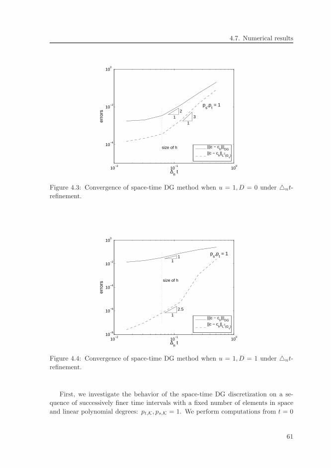
4.7. Numerical results
10−2
10−1
100
10−4
10−2
100
∆n t
erro
rsp
s,p
t = 1
12
1
3
size of h |||c − ch|||
DG||c − c
h||
L2(Ω
T)
Figure 4.3: Convergence of space-time DG method when u = 1, D = 0 under nt-
refinement.
10−2
10−1
100
10−8
10−6
10−4
10−2
100
∆n t
erro
rs
ps,p
t = 1
11
12.5
size of h
|||c − ch|||
DG||c − c
h||
L2(Ω
T)
Figure 4.4: Convergence of space-time DG method when u = 1, D = 1 under nt-
refinement.
First, we investigate the behavior of the space-time DG discretization on a se-
quence of successively finer time intervals with a fixed number of elements in space
and linear polynomial degrees: pt,K, ps,K = 1. We perform computations from t = 0
61
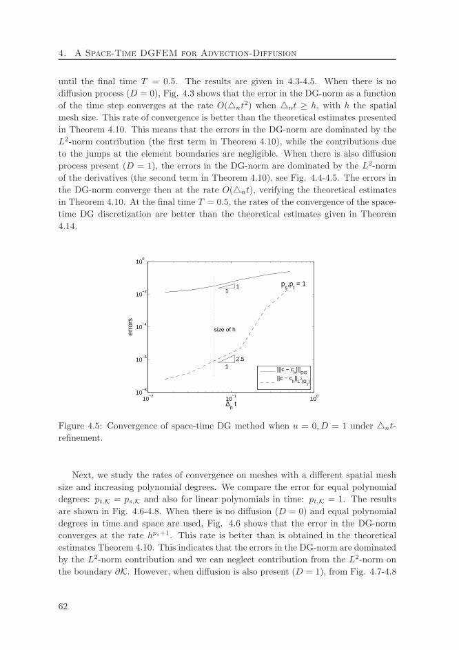
4. A Space-Time DGFEM for Advection-Diffusion
until the final time T = 0.5. The results are given in 4.3-4.5. When there is no
diffusion process (D = 0), Fig. 4.3 shows that the error in the DG-norm as a function
of the time step converges at the rate O(nt2) when nt ≥ h, with h the spatial
mesh size. This rate of convergence is better than the theoretical estimates presented
in Theorem 4.10. This means that the errors in the DG-norm are dominated by the
L2-norm contribution (the first term in Theorem 4.10), while the contributions due
to the jumps at the element boundaries are negligible. When there is also diffusion
process present (D = 1), the errors in the DG-norm are dominated by the L2-norm
of the derivatives (the second term in Theorem 4.10), see Fig. 4.4-4.5. The errors in
the DG-norm converge then at the rate O(nt), verifying the theoretical estimates
in Theorem 4.10. At the final time T = 0.5, the rates of the convergence of the space-
time DG discretization are better than the theoretical estimates given in Theorem
4.14.
10−2
10−1
100
10−8
10−6
10−4
10−2
100
∆n t
erro
rs
ps,p
t = 1
11
12.5
size of h
|||c − ch|||
DG||c − c
h||
L2(Ω
T)
Figure 4.5: Convergence of space-time DG method when u = 0, D = 1 under nt-
refinement.
Next, we study the rates of convergence on meshes with a different spatial mesh
size and increasing polynomial degrees. We compare the error for equal polynomial
degrees: pt,K = ps,K and also for linear polynomials in time: pt,K = 1. The results
are shown in Fig. 4.6-4.8. When there is no diffusion (D = 0) and equal polynomial
degrees in time and space are used, Fig. 4.6 shows that the error in the DG-norm
converges at the rate hps+1. This rate is better than is obtained in the theoretical
estimates Theorem 4.10. This indicates that the errors in the DG-norm are dominated
by the L2-norm contribution and we can neglect contribution from the L2-norm on
the boundary ∂K. However, when diffusion is also present (D = 1), from Fig. 4.7-4.8
62
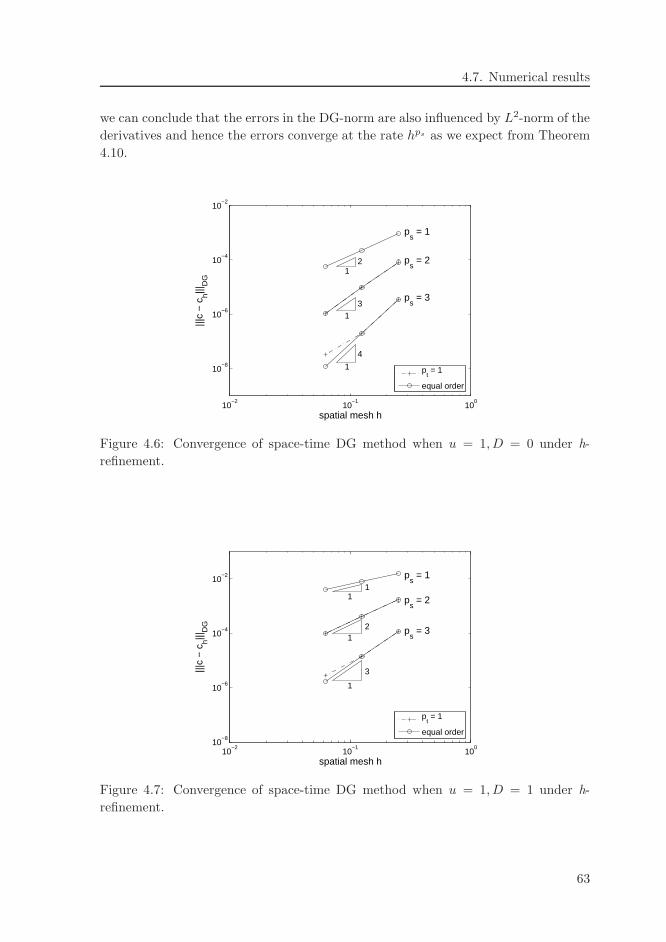
4.7. Numerical results
we can conclude that the errors in the DG-norm are also influenced by L2-norm of the
derivatives and hence the errors converge at the rate hps as we expect from Theorem
4.10.
10−2
10−1
100
10−8
10−6
10−4
10−2
spatial mesh h
|||c
− c
h|||D
G
ps = 1
ps = 2
ps = 3
12
13
1
4
pt = 1
equal order
Figure 4.6: Convergence of space-time DG method when u = 1, D = 0 under h-
refinement.
10−2
10−1
100
10−8
10−6
10−4
10−2
spatial mesh h
|||c
− c
h|||D
G
ps = 1
ps = 2
ps = 3
11
12
1
3
pt = 1
equal order
Figure 4.7: Convergence of space-time DG method when u = 1, D = 1 under h-
refinement.
63
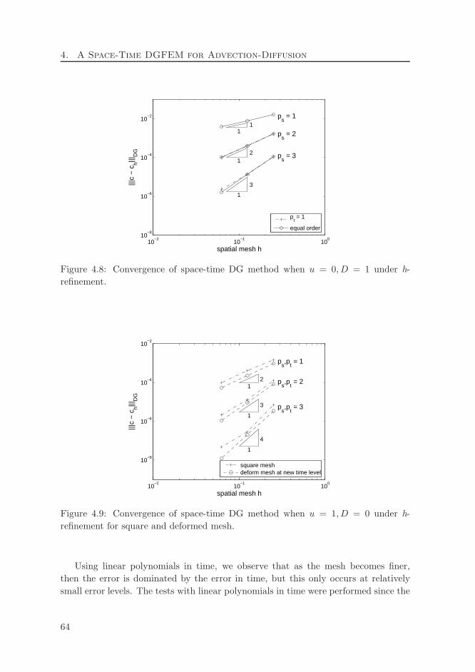
4. A Space-Time DGFEM for Advection-Diffusion
10−2
10−1
100
10−8
10−6
10−4
10−2
spatial mesh h
|||c
− c
h|||D
G
ps = 1
ps = 2
ps = 3
11
12
1
3
pt = 1
equal order
Figure 4.8: Convergence of space-time DG method when u = 0, D = 1 under h-
refinement.
10−2
10−1
100
10−8
10−6
10−4
10−2
spatial mesh h
|||c
− c
h|||D
G
ps,p
t = 1
ps,p
t = 2
ps,p
t = 3
12
1
3
1
4
square meshdeform mesh at new time level
Figure 4.9: Convergence of space-time DG method when u = 1, D = 0 under h-
refinement for square and deformed mesh.
Using linear polynomials in time, we observe that as the mesh becomes finer,
then the error is dominated by the error in time, but this only occurs at relatively
small error levels. The tests with linear polynomials in time were performed since the
64
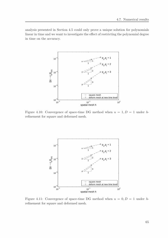
4.7. Numerical results
analysis presented in Section 4.5 could only prove a unique solution for polynomials
linear in time and we want to investigate the effect of restricting the polynomial degree
in time on the accuracy.
10−2
10−1
100
10−8
10−6
10−4
10−2
spatial mesh h
|||c
− c
h|||D
G
ps,p
t = 1
ps,p
t = 2
ps,p
t = 3
11
12
1
3
square meshdeform mesh at new time level
Figure 4.10: Convergence of space-time DG method when u = 1, D = 1 under h-
refinement for square and deformed mesh.
10−2
10−1
100
10−8
10−6
10−4
10−2
spatial mesh h
|||c
− c
h|||D
G
ps,p
t = 1
ps,p
t = 2
ps,p
t = 3
11
12
1
3
square meshdeform mesh at new time level
Figure 4.11: Convergence of space-time DG method when u = 0, D = 1 under h-
refinement for square and deformed mesh.
65
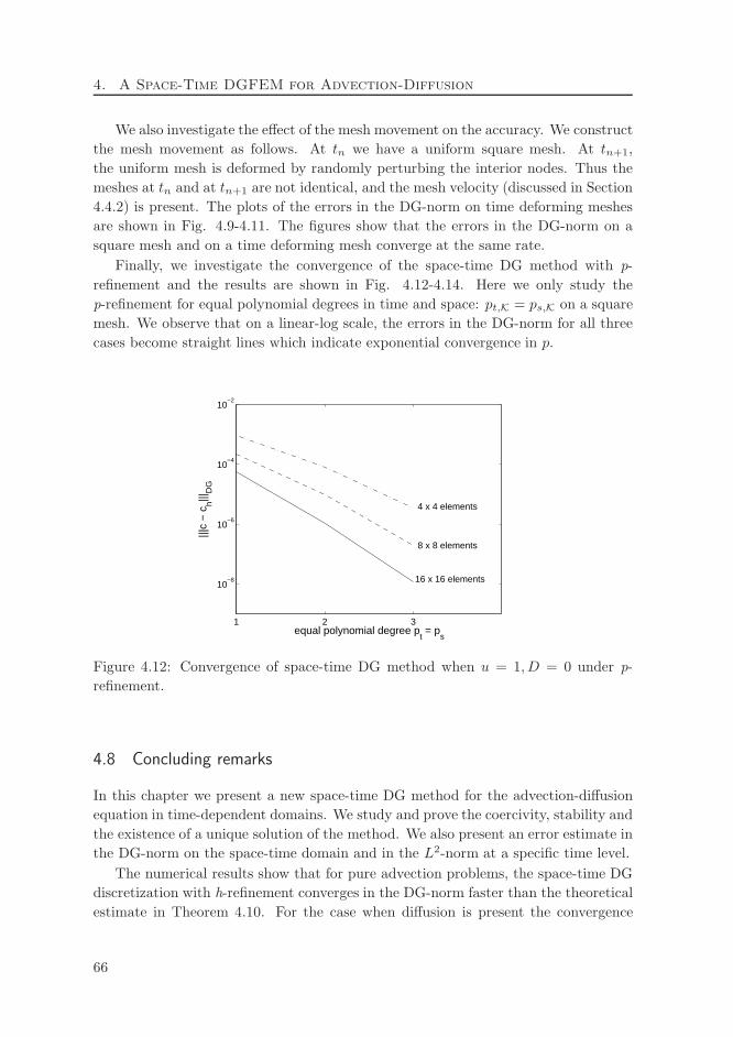
4. A Space-Time DGFEM for Advection-Diffusion
We also investigate the effect of the mesh movement on the accuracy. We construct
the mesh movement as follows. At tn we have a uniform square mesh. At tn+1,
the uniform mesh is deformed by randomly perturbing the interior nodes. Thus the
meshes at tn and at tn+1 are not identical, and the mesh velocity (discussed in Section
4.4.2) is present. The plots of the errors in the DG-norm on time deforming meshes
are shown in Fig. 4.9-4.11. The figures show that the errors in the DG-norm on a
square mesh and on a time deforming mesh converge at the same rate.
Finally, we investigate the convergence of the space-time DG method with p-
refinement and the results are shown in Fig. 4.12-4.14. Here we only study the
p-refinement for equal polynomial degrees in time and space: pt,K = ps,K on a square
mesh. We observe that on a linear-log scale, the errors in the DG-norm for all three
cases become straight lines which indicate exponential convergence in p.
1 2 3
10−8
10−6
10−4
10−2
equal polynomial degree pt = p
s
|||c
− c
h|||D
G
4 x 4 elements
8 x 8 elements
16 x 16 elements
Figure 4.12: Convergence of space-time DG method when u = 1, D = 0 under p-
refinement.
4.8 Concluding remarks
In this chapter we present a new space-time DG method for the advection-diffusion
equation in time-dependent domains. We study and prove the coercivity, stability and
the existence of a unique solution of the method. We also present an error estimate in
the DG-norm on the space-time domain and in the L2-norm at a specific time level.
The numerical results show that for pure advection problems, the space-time DG
discretization with h-refinement converges in the DG-norm faster than the theoretical
estimate in Theorem 4.10. For the case when diffusion is present the convergence
66
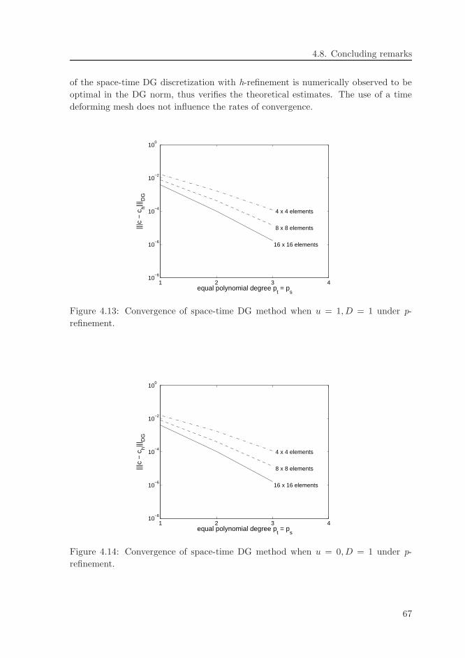
4.8. Concluding remarks
of the space-time DG discretization with h-refinement is numerically observed to be
optimal in the DG norm, thus verifies the theoretical estimates. The use of a time
deforming mesh does not influence the rates of convergence.
1 2 3 410
−8
10−6
10−4
10−2
100
equal polynomial degree pt = p
s
|||c
− c
h|||D
G
4 x 4 elements
8 x 8 elements
16 x 16 elements
Figure 4.13: Convergence of space-time DG method when u = 1, D = 1 under p-
refinement.
1 2 3 410
−8
10−6
10−4
10−2
100
equal polynomial degree pt = p
s
|||c
− c
h|||D
G
4 x 4 elements
8 x 8 elements
16 x 16 elements
Figure 4.14: Convergence of space-time DG method when u = 0, D = 1 under p-
refinement.
67
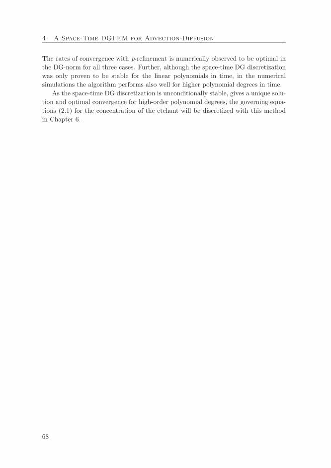
4. A Space-Time DGFEM for Advection-Diffusion
The rates of convergence with p-refinement is numerically observed to be optimal in
the DG-norm for all three cases. Further, although the space-time DG discretization
was only proven to be stable for the linear polynomials in time, in the numerical
simulations the algorithm performs also well for higher polynomial degrees in time.
As the space-time DG discretization is unconditionally stable, gives a unique solu-
tion and optimal convergence for high-order polynomial degrees, the governing equa-
tions (2.1) for the concentration of the etchant will be discretized with this method
in Chapter 6.
68
Chapter 5
A Space-Time Discontinuous Galerkin Method for
Incompressible Flows
5.1 Introduction
In this chapter we discuss a space-time DG discretization for the incompressible
Navier-Stokes equations, which are the governing equations for the velocity and pres-
sure field in the acid fluid, see (2.6). The algorithm is closely related to the DG
discretization developed by Cockburn, Kanschat, and Schotzau, which is discussed in
a series of papers [21, 22, 23, 24]. Also, the analysis in [54, 55] provides important
information on the construction of DG algorithms for incompressible flows. A dif-
ferent approach using approximate Riemann solvers for the artificial compressibility
pertubation of the incompressible Navier-Stokes equations is provided in [8], but this
technique only applies to steady flows.
There are four important points that have to be considered in the development
of a DG discretization for the incompressible Navier-Stokes equations. Each one is
shortly discussed here together with what has been studied in the literature for the
steady-state case.
The first issue is the treatment of the nonlinearity in the convective term. There
are several ways to deal with this nonlinear term. In [24] the nonlinear incompressible
Navier-Stokes equations are linearized by applying a Picard linearization to obtain
a sequence of Oseen equations. This sequence of Oseen equations is then solved
iteratively. An alternative technique is to solve the nonlinear equations directly using
a Newton method, such as done in [8]. This requires, however, a careful linearization
of all terms which is non-trivial when the solution of the Navier-Stokes equations
must be coupled with more complicated models for the chemical reactions in the
wet-chemical etching process.
The second issue is the DG discretization of the viscous terms. The obvious
choice is to discretize the viscous terms in a similar way as done for elliptic equations
69
5. A Space-Time DGFEM for Incompressible Flows
(see Chapter 3), but now extended to vector functions. In [8], the Bassi and Rebay
method (Method 4 in Table 3.1) is used, while the LDG method (Method 2 in Table
3.1) is used in [21, 22, 23, 24]. Based on our experience with the advection-diffusion
equation, discussed in Chapter 4, we will use the Bassi and Rebay method for the
viscous contribution.
The third issue is the incompressibility constraint imposed by the continuity equa-
tion. In [24], the mean values are chosen as the numerical flux at the element faces
in the continuity equation. In order to have a globally divergence-free velocity field,
a post processing operator is then used to project the velocity field onto the space of
globally divergence-free functions. Another approach, presented in [8], is to add an
artificial compressibility term to the continuity equation. The numerical flux at the
element faces is provided by the solution of a Riemann problem. This algorithm is,
however, limited to steady flows.
The fourth issue is the pressure stabilization. The analysis presented in [54, 55]
discusses the importance of the pressure stabilization operator for the choice of the
polynomial degrees in the approximations of the velocity and pressure. Without a
stabilization term, the DG method can only be proven stable when the polynomial
degree used in the approximation of the pressure is one less than the polynomial
degree for the approximation of the velocity. By adding a stabilization term similar
to the one used for the elliptic equations, stability is proven when equal polynomial
degrees are used for both the velocity and the pressure.
The above issues are also of direct interest for a space-time DG discretization
of the incompressible Navier-Stokes equations. To deal with the nonlinear term, we
follow the approach in which the nonlinear problem is linearized as an Oseen equation.
This is discussed in Section 5.2. After the introduction of the finite element spaces
and trace operators in Section 5.3, we give the derivation of the space-time DG weak
formulation for the Oseen equations in time-dependent domains in Section 5.4. The
discretization of the viscous terms follows the space-time DG discretization in Chapter
4. Two approaches for the stabilization term are considered, which are similar to
the stabilization operators for the elliptic equations discussed in Chapter 3. The
analysis of the stability of the space-time DG discretization for the Oseen equations
is presented in Section 5.5. Some numerical experiments are given in Section 5.6.
5.2 The incompressible flows
In this section we recapitulate the Navier-Stokes equations given for incompressible
flows and set some notations. We follow the description given in [32].
Let Ωt be an open, bounded, time-dependent domain in Rd at time t, where d is
the number of spatial dimensions. The closure of Ωt is Ωt and the boundary of Ωt is
denoted by ∂Ωt. Denoting x = (x1, . . . , xd) as the spatial variables, we consider the
70
5.2. The incompressible flows
time-dependent incompressible Navier-Stokes equations for the velocity field u ∈ Rd
and the kinematic pressure p := p/ρ ∈ R in the domain Ωt:
∂u
∂t+∇ · (u⊗ u)− ν∇ · ∇u+∇p = f, in Ωt, (5.1a)
∇ · u = 0, in Ωt, (5.1b)
where ν ∈ R+ is the kinematic viscosity and f ∈ Rd the force vector. We introduce
the product between two vectors a ∈ Rm, b ∈ Rn as a ⊗ b ∈ Rm×n with elements
(a⊗ b)ij = aibj. The notation ∇ is used for the spatial gradient operator in Rd, and
defined as ∇ =(
∂∂x1
, . . . , ∂∂xd
). We also define the divergence of a tensor A ∈ R
m×n
as: ∇ ·A =∑
j∂
∂xjAij .
As mentioned in the introduction, we linearize (5.1) using a Picard linearization.
This results in the Oseen equations:
∂u
∂t+∇ · (u⊗ w) − ν∇ · ∇u+∇p = f, in Ωt, (5.2a)
∇ · u = 0, in Ωt, (5.2b)
with w ∈ Rd a given convective divergence free velocity field.
For the space-time discretization, we consider the Oseen equations directly in a
domain in Rd+1. A point x ∈ Rd+1 has coordinates (x0, x), with x0 = t representing
time. We define the space-time domain E ⊂ Rd+1. The boundary of the space-time
domain ∂E consists of the hypersurfaces Ω0 := x ∈ ∂E | x0 = 0, ΩT := x ∈ ∂E |x0 = T , and Q := x ∈ ∂E | 0 < x0 < T . Introducing the gradient operator in
Rd+1 as ∇ =
(∂
∂x0, ∂
∂x1, . . . , ∂
∂xd
)and the vector C = (1, w), the Oseen equations (5.2)
can be transformed into a space-time formulation as:
∇ · (u⊗ C)− ν∇ · ∇u+∇ · (Id p) = f, in E , (5.3a)
∇ · u = 0, in E , (5.3b)
with Id the d× d identity matrix.
Since different boundary conditions are imposed on ∂E , we discuss the subdivision
of ∂E into different parts. The boundary ∂E is divided into disjoint subsets Γm and
Γp, with:
Γm := x ∈ ∂E : C · n < 0, Γp := x ∈ ∂E : C · n ≥ 0.The subscripts m and p denote the inflow and outflow boundaries, respectively. We
subdivide Γm further into two sets: ΓDm and Ω0, with ΓDm the part of Γm with a
Dirichlet boundary condition and Ω0 the part of Γm with the initial condition. The
part Γp is divided into three sets: ΩT , ΓDp and ΓN , with ΩT the part of ∂E at the
final time T , ΓDp the part of Γp with a Dirichlet boundary condition and ΓN the
part of Γp with a Neumann boundary condition. Note that ΓD = ΓDm ∪ ΓDp is the
71
5. A Space-Time DGFEM for Incompressible Flows
part of the space-time boundary with a Dirichlet boundary condition. The boundary
conditions on different parts of ∂E are written as
u = u0 on Ω0, (5.4a)
u = gD on ΓD, (5.4b)
n · ∇u = gN on ΓN , (5.4c)
p = pN on ΓN , (5.4d)
with u0 a given initial function and gD, gN , pN given functions defined on the bound-
ary. There is no boundary condition imposed on ΩT .
5.3 Space-time elements, finite element spaces and trace operators
5.3.1 Definition of space-time slabs, elements and faces
The description of the space-time slabs and the construction of the space-time ele-
ments in this section follows the definitions given in Section 4.3.1. As already intro-
duced in the previous section, we consider the problem in a space-time domain E .The nth time interval is denoted by In, with its length defined as nt = tn+1 − tn.
A space-time slab is defined as the domain En = E ∩ (In × Rd) with boundaries Ωtn
,
Ωtn+1 and Qn = ∂En \ (Ωtn∪ Ωtn+1).
The space-time element is denoted by K, with hK the radius of the smallest sphere
containing each element K. The element boundary ∂K is the union of open faces of K,
which contains three parts Kn,Kn+1, and QnK = ∂K\(Kn∪Kn+1). We denote by nK
the unit outward space-time normal vector on ∂K. The definition of the space-time
domain is completed with the tessellation T nh in each space-time slab and Th = ∪nT n
h
in the space-time domain.
We consider several sets of faces S. The set of all faces in E is denoted with F , the
set of all interior faces in E with Fint, and the set of all boundary faces on ∂E with
Fbnd. In the space-time slab En we denote the set of all faces with Fn and the set
of all interior faces with SnI . The faces separating two space-time slabs are denoted
as SnS . Several sets of boundary faces are defined as follows. The set of faces with a
Dirichlet boundary condition is denoted with SnD. This set can be divided further into
sets SnDm and Sn
Dp, which correspond to the faces with a Dirichlet boundary condition
on Γm and Γp, respectively. The set of faces with a Neumann boundary condition is
denoted with SnN . Further, the sets Sn
I and SnD are grouped into Sn
ID and the sets
SnI ,Sn
D and SnN are grouped into Sn
IDN .
5.3.2 Finite element spaces and trace operators
The definitions of the anisotropic Sobolev spaces and the broken Sobolev spaces which
are given in Section 4.3.2, with their corresponding norms and semi-norms, can be
72
5.3. Space-time elements, FE spaces and trace operators
straightforwardly extended to vector and tensor functions. For simplicity then the
anisotropic Sobolev spaces that we discuss in this chapter follow the definition in
Section 4.3.2.
We now discuss the finite element spaces associated with the tessellation Th that
will be used in this chapter. To each element K we assign a pair of nonnegative
integers (pt,K, ps,K) as local polynomial degrees, where the subscripts t and s denote
time and space, respectively, and collect them into vectors pt = pt,K : K ∈ Thand ps = ps,K : K ∈ Th. We define Qpt,K,ps,K
(K) as the set of all tensor-product
polynomials on K of degree pt,K in the time direction and degree ps,K in each spatial
coordinate direction. The finite element spaces of discontinuous polynomial functions
are defined as follows
V(pt,ps)h := v ∈ L2(E)d : v|K QK FK ∈ [Q(pt,K,ps,K)(K)]d, ∀K ∈ Th,Q(pt,ps)
h := q ∈ L2(E) : q|K QK FK ∈ Q(pt,K,ps,K)(K), ∀K ∈ Th.
In the derivation and analysis of the numerical discretization we also make use of
auxiliary spaces Σ(pt,ps)h and Σ
(pt,ps)h :
Σ(pt,ps)h := τ ∈ L2(E)d×(d+1) : τ |K QK FK ∈ [Q(pt,K,ps,K)(K)]d×(d+1), ∀K ∈ Th,
Σ(pt,ps)h := τ ∈ L2(E)d×d : τ |K QK FK ∈ [Q(pt,K,ps,K)(K)]d×d, ∀K ∈ Th.
The so called traces of v ∈ V (pt,ps)h on ∂K are defined as: v±K = limǫ↓0 v(x ± ǫnK).
The traces of q ∈ Q(pt,ps)h , τ ∈ Σ
(pt,ps)h , and τ ∈ Σ
(pt,ps)h are defined similarly.
Next, we define several trace operators for the sets Fint and Fbnd. Note that func-
tions v ∈ V (pt,ps)h , q ∈ Q(pt,ps)
h , τ ∈ Σ(pt,ps)h and τ ∈ Σ
(pt,ps)h are in general multivalued
on a face S ∈ Fint. Introducing the functions vi := v|Ki, qi := q|Ki
, τi := τ |Ki, τi :=
τ |Ki, we define the average operator · on S ∈ Fint as:
v = (vi + vj)/2, q = (qi + qj)/2, τ = (τi + τj)/2, τ = (τi + τj)/2,
while on S ∈ Fbnd, we set accordingly
v = v, q = q, τ = τ, τ = τ .
We also introduce the jump operators [[·]] and 〈〈·〉〉. For functions q ∈ Q(pt,ps)h ,
τ ∈ Σ(pt,ps)h and τ ∈ Σ
(pt,ps)h , the jump operators are defined on S ∈ Fint as:
[[q]] = qini + qjnj , [[τ ]] = τi · ni + τj · nj ,
〈〈q〉〉 = qini + qj nj , 〈〈τ〉〉 = τi · ni + τj · nj ,
with ni, ni the outward normal vector on ∂Ki and its spatial part. For functions
v ∈ V (pt,ps)h , we define the jump operators on S ∈ Fint as follows:
[[[v]]] = vi ⊗ ni + vj ⊗ nj, 〈〈〈v〉〉〉 = vi ⊗ ni + vj ⊗ nj , 〈〈v〉〉 = vi · ni + vj · nj .
73
5. A Space-Time DGFEM for Incompressible Flows
By taking all functions from the neighboring element equal to zero, the definitions of
jump operators are also valid on boundary faces S ∈ Fbnd. Note that 〈〈v〉〉 is scalar,
[[q]] ∈ Rd+1, 〈〈q〉〉 ∈ Rd are vectors, and [[[v]]] ∈ Rd×(d+1), 〈〈〈v〉〉〉 ∈ Rd×d are matrices.
The jumps [[τ ]], 〈〈τ 〉〉 ∈ Rd are also vectors.
5.3.3 Lifting operators
The derivation of the space-time DG formulation in this chapter requires several lifting
operators. In this section we introduce lifting operators for vector functions.
First, we introduce the lifting operator LS : (L2(S))d×(d+1) → Σ(pt,ps)h :
∫
ELS(ϑ) : τ dE =
∫
S
ϑ : τ dS, ∀τ ∈ Σ(pt,ps)h , ∀S ∈ ∪nSn
ID, (5.5)
where the dyadic product between two matrices A,B ∈ Rm×n is defined as: A : B =∑m
i=1
∑nj=1 AijBij . The global lifting operator L : (L2(∪nSn
ID))d×(d+1) → Σ(pt,ps)h is
then introduced as∫
EL(ϑ) : τ dE =
∑
S∈∪nSnID
∫
ELS(ϑ) : τ dE , ∀τ ∈ Σ
(pt,ps)h . (5.6)
We specify the above lifting operators for the Dirichlet boundary condition, using
a similar argument as in Section 4.3.3. On faces S ∈ ∪nSnD we have
∫
ELS(PgD ⊗ n) : τ dE =
∫
S
gD ⊗ n : τ dS, ∀τ ∈ Σ(pt,ps)h , ∀S ∈ ∪nSn
D, (5.7)
with P the L2 projection on Σ(pt,ps)h . For the global lifting operators, we proceed also
as in Section 4.3.3. We replace ϑ by PgD⊗n in (5.5) and (5.6) to obtain the following
global lifting operator for the Dirichlet boundary:∫
EL(PgD ⊗ n) : τ dE =
∑
S∈∪nSnD
∫
S
gD ⊗ n : τ dS, ∀τ ∈ Σ(pt,ps)h . (5.8)
Using (5.6) and (5.8), we then introduce LID : (L2(∪nSnID))d×(d+1) → Σ
(pt,ps)h as:
LID(ϑ) = −L(ϑ) + L(PgD ⊗ n). (5.9)
Later in this chapter, we will also use the spatial part of the lifting operators, denoted
by L, LS , which are obtained by eliminating the first component of L,LS , respectively.
5.4 Space-time DG discretization for the Oseen equations
In this section we give a derivation of the space-time DG weak formulation for the
Oseen equations (5.3). As in Chapter 4, we introduce an auxiliary variable σ = ∇u,
74
5.4. Space-time DG for Oseen equations
to obtain the following system of first order equations:
σ = ∇u, in E , (5.10a)
∇ · (u ⊗ C)− ν∇ · σ +∇ · (Id p) = f, in E , (5.10b)
∇ · u = 0, in E , (5.10c)
together with the boundary conditions (5.4a)-(5.4d). We assume that the convective
velocity field w in the vector C is in the space:
Jh := v ∈ L2(E)d,∇ · v = 0 andv |K∈ H0,1(K)d, ∀K ∈ Th.
In the next three sections we give the derivation of the weak formulation for (5.10).
5.4.1 Weak formulation for the auxiliary variable
First, we consider the auxiliary variable (5.10a). Multiplying (5.10a) with an arbitrary
test function τ ∈ Σ(pt,ps)h and integrating over an element K ∈ T n
h , we obtain:∫
Kσ : τ dK =
∫
K∇u : τ dK, ∀τ ∈ Σ
(pt,ps)h . (5.11)
Next, we substitute σ, u with their approximations σh ∈ Σ(pt,ps)h , uh ∈ V (pt,ps)
h and
perform integration by parts on the right hand side of (5.11) twice with respect to
x1, . . . , xd. After summation over all elements K ∈ T nh , we obtain for all τ ∈ Σ
(pt,ps)h :
∫
En
σh : τ dE =
∫
En
∇huh : τ dE +∑
K∈T nh
∫
QnK
(uσh − uh)⊗ n : τ d∂K. (5.12)
The variable uσh is the numerical flux that must be defined to account for the mul-
tivalued trace at QnK. Note that since we perform the integration by parts on the
spatial variables, we only have to consider the weak formulation in the space-time
slab En since there are no fluxes between different space-time slabs.
We recall the following relation, which is an extension of the identity introduced
in [4] for tensors τ and vectors v, piecewise smooth on Th:
∑
K∈T nh
∫
QnK
v ⊗ n : τ d∂K =∑
S∈SnIDN
∫
S
〈〈〈v〉〉〉 : τ dS +∑
S∈SnI
∫
S
v · 〈〈τ 〉〉 dS, (5.13)
and can be proved by a straightforward calculation. When applied to the last term
in (5.12), this results in
∑
K∈T nh
∫
QnK
(uσh − uh)⊗ n : τ d∂K =
∑
S∈SnIDN
∫
S
〈〈〈uσh − uh〉〉〉 : τ dS
+∑
S∈SnI
∫
S
uσh − uh · 〈〈τ 〉〉 dS. (5.14)
75
5. A Space-Time DGFEM for Incompressible Flows
We consider now the choice for numerical flux uσh. We make a similar choice as in
Section 4.4.1, but now applied to vector functions:
uσh = uh on Sn
I , uσh = gD on Sn
D, uσh = uh on Sn
N . (5.15)
Replacing uσh in (5.14) with the choices for the numerical flux (5.15), we obtain:
∑
K∈T nh
∫
QnK
(uσh − uh)⊗ n : τ d∂K =−
∑
S∈SnID
∫
S
〈〈〈uh〉〉〉 :τ dS
+∑
S∈SnD
∫
S
gD ⊗ n : τ dS. (5.16)
The weak formulation (5.12) is now equal to:
Find a σh ∈ Σ(pt,ps)h , such that for all τ ∈ Σ
(pt,ps)h , the following relation is satisfied:
∫
En
σh : τ dE =
∫
En
∇huh : τ dE−∑
S∈SnID
∫
S
〈〈〈uh〉〉〉 :τ dS+∑
S∈SnD
∫
S
gD⊗n : τ dS. (5.17)
We sum now (5.17) over all space-time slabs. The last two terms on the right hand
side of (5.17) are then replaced with the spatial part of the lifting operator LID,
defined in (5.9), to obtain:
∫
En
LID(〈〈〈uh〉〉〉) : τ dE = −∑
S∈SnID
∫
S
〈〈〈uh〉〉〉 :τ dS +∑
S∈SnD
∫
S
gD ⊗ n : τ dS. (5.18)
Using (5.18) into (5.17), we can express σh ∈ Σ(pt,ps)h as
σh = ∇huh + LID(〈〈〈uh〉〉〉), a.e. ∀x ∈ E . (5.19)
This relation will be used in the next section to eliminate the auxiliary variable from
the DG discretization.
5.4.2 Weak formulation for the primal variables
In this section we derive the weak formulation for (5.10b). First we multiply (5.10b)
with arbitrary test functions v ∈ V (pt,ps)h and integrate over the element K, such that
for all v ∈ V (pt,ps)h the following relation is satisfied:
∫
K(∇ · (u⊗C)) · v dK−
∫
K(ν∇ ·σ) · v dK+
∫
K(∇ · Id p) · v dK =
∫
Kf · v dK. (5.20)
The functions u, σ, p are then substituted by their approximations uh ∈ V (pt,ps)h , σh ∈
Σ(pt,ps)h , ph ∈ Q(pt,ps)
h , respectively. Next, we integrate by parts each term on the
left hand side of (5.20). For the first term, integration by parts is with respect to
76
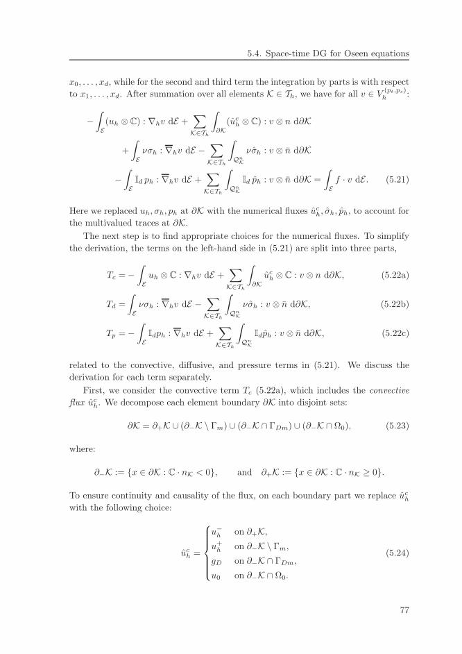
5.4. Space-time DG for Oseen equations
x0, . . . , xd, while for the second and third term the integration by parts is with respect
to x1, . . . , xd. After summation over all elements K ∈ Th, we have for all v ∈ V (pt,ps)h :
−∫
E(uh ⊗ C) : ∇hv dE +
∑
K∈Th
∫
∂K(uc
h ⊗ C) : v ⊗ n d∂K
+
∫
Eνσh : ∇hv dE −
∑
K∈Th
∫
QnK
νσh : v ⊗ n d∂K
−∫
EId ph : ∇hv dE +
∑
K∈Th
∫
QnK
Id ph : v ⊗ n d∂K =
∫
Ef · v dE . (5.21)
Here we replaced uh, σh, ph at ∂K with the numerical fluxes uch, σh, ph, to account for
the multivalued traces at ∂K.
The next step is to find appropriate choices for the numerical fluxes. To simplify
the derivation, the terms on the left-hand side in (5.21) are split into three parts,
Tc =−∫
Euh ⊗ C : ∇hv dE +
∑
K∈Th
∫
∂Kuc
h ⊗ C : v ⊗ n d∂K, (5.22a)
Td =
∫
Eνσh : ∇hv dE −
∑
K∈Th
∫
QnK
νσh : v ⊗ n d∂K, (5.22b)
Tp =−∫
EIdph : ∇hv dE +
∑
K∈Th
∫
QnK
Idph : v ⊗ n d∂K, (5.22c)
related to the convective, diffusive, and pressure terms in (5.21). We discuss the
derivation for each term separately.
First, we consider the convective term Tc (5.22a), which includes the convective
flux uch. We decompose each element boundary ∂K into disjoint sets:
∂K = ∂+K ∪ (∂−K \ Γm) ∪ (∂−K ∩ ΓDm) ∪ (∂−K ∩ Ω0), (5.23)
where:
∂−K := x ∈ ∂K : C · nK < 0, and ∂+K := x ∈ ∂K : C · nK ≥ 0.
To ensure continuity and causality of the flux, on each boundary part we replace uch
with the following choice:
uch =
u−h on ∂+K,u+
h on ∂−K \ Γm,
gD on ∂−K ∩ ΓDm,
u0 on ∂−K ∩ Ω0.
(5.24)
77
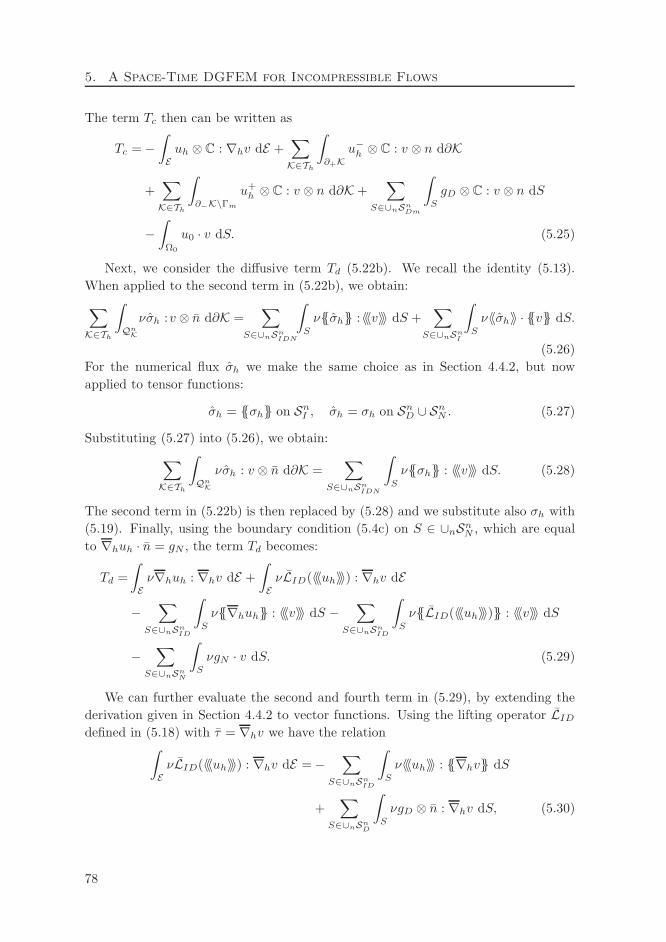
5. A Space-Time DGFEM for Incompressible Flows
The term Tc then can be written as
Tc =−∫
Euh ⊗ C : ∇hv dE +
∑
K∈Th
∫
∂+Ku−h ⊗ C : v ⊗ n d∂K
+∑
K∈Th
∫
∂−K\Γm
u+h ⊗ C : v ⊗ n d∂K +
∑
S∈∪nSnDm
∫
S
gD ⊗ C : v ⊗ n dS
−∫
Ω0
u0 · v dS. (5.25)
Next, we consider the diffusive term Td (5.22b). We recall the identity (5.13).
When applied to the second term in (5.22b), we obtain:
∑
K∈Th
∫
QnK
νσh :v ⊗ n d∂K =∑
S∈∪nSnIDN
∫
S
νσh :〈〈〈v〉〉〉 dS +∑
S∈∪nSnI
∫
S
ν〈〈σh〉〉 · v dS.
(5.26)
For the numerical flux σh we make the same choice as in Section 4.4.2, but now
applied to tensor functions:
σh = σh on SnI , σh = σh on Sn
D ∪ SnN . (5.27)
Substituting (5.27) into (5.26), we obtain:
∑
K∈Th
∫
QnK
νσh : v ⊗ n d∂K =∑
S∈∪nSnIDN
∫
S
νσh : 〈〈〈v〉〉〉 dS. (5.28)
The second term in (5.22b) is then replaced by (5.28) and we substitute also σh with
(5.19). Finally, using the boundary condition (5.4c) on S ∈ ∪nSnN , which are equal
to ∇huh · n = gN , the term Td becomes:
Td =
∫
Eν∇huh : ∇hv dE +
∫
EνLID(〈〈〈uh〉〉〉) : ∇hv dE
−∑
S∈∪nSnID
∫
S
ν∇huh : 〈〈〈v〉〉〉 dS −∑
S∈∪nSnID
∫
S
νLID(〈〈〈uh〉〉〉) : 〈〈〈v〉〉〉 dS
−∑
S∈∪nSnN
∫
S
νgN · v dS. (5.29)
We can further evaluate the second and fourth term in (5.29), by extending the
derivation given in Section 4.4.2 to vector functions. Using the lifting operator LID
defined in (5.18) with τ = ∇hv we have the relation∫
EνLID(〈〈〈uh〉〉〉) : ∇hv dE =−
∑
S∈∪nSnID
∫
S
ν〈〈〈uh〉〉〉 : ∇hv dS
+∑
S∈∪nSnD
∫
S
νgD ⊗ n : ∇hv dS, (5.30)
78
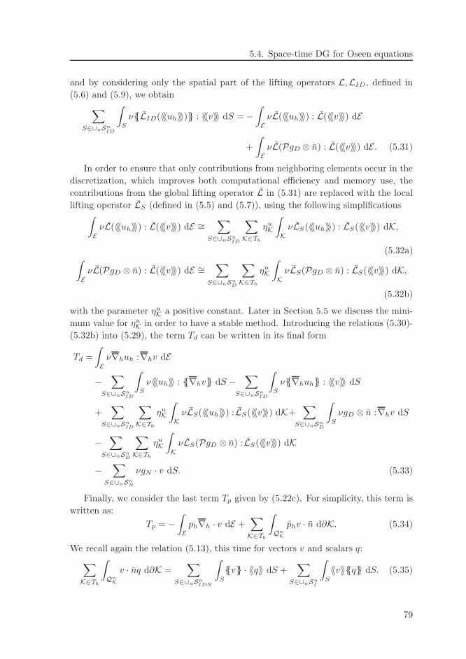
5.4. Space-time DG for Oseen equations
and by considering only the spatial part of the lifting operators L,LID, defined in
(5.6) and (5.9), we obtain
∑
S∈∪nSnID
∫
S
νLID(〈〈〈uh〉〉〉) : 〈〈〈v〉〉〉 dS =−∫
EνL(〈〈〈uh〉〉〉) : L(〈〈〈v〉〉〉) dE
+
∫
EνL(PgD ⊗ n) : L(〈〈〈v〉〉〉) dE . (5.31)
In order to ensure that only contributions from neighboring elements occur in the
discretization, which improves both computational efficiency and memory use, the
contributions from the global lifting operator L in (5.31) are replaced with the local
lifting operator LS (defined in (5.5) and (5.7)), using the following simplifications∫
EνL(〈〈〈uh〉〉〉) : L(〈〈〈v〉〉〉) dE ∼=
∑
S∈∪nSnID
∑
K∈Th
ηuK
∫
KνLS(〈〈〈uh〉〉〉) : LS(〈〈〈v〉〉〉) dK,
(5.32a)∫
EνL(PgD ⊗ n) : L(〈〈〈v〉〉〉) dE ∼=
∑
S∈∪nSnD
∑
K∈Th
ηuK
∫
KνLS(PgD ⊗ n) : LS(〈〈〈v〉〉〉) dK,
(5.32b)
with the parameter ηuK a positive constant. Later in Section 5.5 we discuss the mini-
mum value for ηuK in order to have a stable method. Introducing the relations (5.30)-
(5.32b) into (5.29), the term Td can be written in its final form
Td =
∫
Eν∇huh :∇hv dE
−∑
S∈∪nSnID
∫
S
ν〈〈〈uh〉〉〉 : ∇hv dS −∑
S∈∪nSnID
∫
S
ν∇huh : 〈〈〈v〉〉〉 dS
+∑
S∈∪nSnID
∑
K∈Th
ηuK
∫
KνLS(〈〈〈uh〉〉〉) : LS(〈〈〈v〉〉〉) dK+
∑
S∈∪nSnD
∫
S
νgD ⊗ n :∇hv dS
−∑
S∈∪nSnD
∑
K∈Th
ηuK
∫
KνLS(PgD ⊗ n) : LS(〈〈〈v〉〉〉) dK
−∑
S∈∪nSnN
νgN · v dS. (5.33)
Finally, we consider the last term Tp given by (5.22c). For simplicity, this term is
written as:
Tp = −∫
Eph∇h · v dE +
∑
K∈Th
∫
QnK
phv · n d∂K. (5.34)
We recall again the relation (5.13), this time for vectors v and scalars q:
∑
K∈Th
∫
QnK
v · nq d∂K =∑
S∈∪nSnIDN
∫
S
v · 〈〈q〉〉 dS +∑
S∈∪nSnI
∫
S
〈〈v〉〉q dS. (5.35)
79
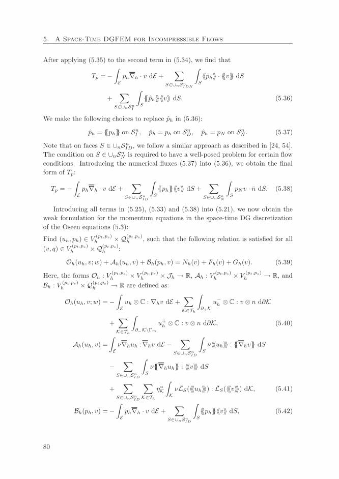
5. A Space-Time DGFEM for Incompressible Flows
After applying (5.35) to the second term in (5.34), we find that
Tp =−∫
Eph∇h · v dE +
∑
S∈∪nSnIDN
∫
S
〈〈ph〉〉 · v dS
+∑
S∈∪nSnI
∫
S
ph〈〈v〉〉 dS. (5.36)
We make the following choices to replace ph in (5.36):
ph = ph on SnI , ph = ph on Sn
D, ph = pN on SnN . (5.37)
Note that on faces S ∈ ∪nSnID, we follow a similar approach as described in [24, 54].
The condition on S ∈ ∪nSnN is required to have a well-posed problem for certain flow
conditions. Introducing the numerical fluxes (5.37) into (5.36), we obtain the final
form of Tp:
Tp = −∫
Eph∇h · v dE +
∑
S∈∪nSnID
∫
S
ph〈〈v〉〉 dS +∑
S∈∪nSnN
∫
S
pNv · n dS. (5.38)
Introducing all terms in (5.25), (5.33) and (5.38) into (5.21), we now obtain the
weak formulation for the momentum equations in the space-time DG discretization
of the Oseen equations (5.3):
Find (uh, ph) ∈ V (pt,ps)h ×Q(pt,ps)
h , such that the following relation is satisfied for all
(v, q) ∈ V (pt,ps)h ×Q(pt,ps)
h :
Oh(uh, v;w) +Ah(uh, v) + Bh(ph, v) = Nh(v) + Fh(v) +Gh(v). (5.39)
Here, the forms Oh : V(pt,ps)h × V (pt,ps)
h × Jh → R, Ah : V(pt,ps)h × V (pt,ps)
h → R, and
Bh : V(pt,ps)h ×Q(pt,ps)
h → R are defined as:
Oh(uh, v;w) =−∫
Euh ⊗ C : ∇hv dE +
∑
K∈Th
∫
∂+Ku−h ⊗ C : v ⊗ n d∂K
+∑
K∈Th
∫
∂−K\Γm
u+h ⊗ C : v ⊗ n d∂K, (5.40)
Ah(uh, v) =
∫
Eν∇huh :∇hv dE −
∑
S∈∪nSnID
∫
S
ν〈〈〈uh〉〉〉 : ∇hv dS
−∑
S∈∪nSnID
∫
S
ν∇huh : 〈〈〈v〉〉〉 dS
+∑
S∈∪nSnID
∑
K∈Th
ηuK
∫
KνLS(〈〈〈uh〉〉〉) : LS(〈〈〈v〉〉〉) dK, (5.41)
Bh(ph, v) =−∫
Eph∇h · v dE +
∑
S∈∪nSnID
∫
S
ph〈〈v〉〉 dS, (5.42)
80
5.4. Space-time DG for Oseen equations
and the linear forms Nh : V(pt,ps)h → R, Fh : V
(pt,ps)h → R, Gh : V
(pt,ps)h → R as:
Nh(v) =−∑
S∈∪nSnDm
∫
S
gD ⊗ C : v ⊗ n dS +
∫
Ω0
u0 · v dS, (5.43)
Fh(v) =−∑
S∈∪nSnD
∫
S
νgD ⊗ n : ∇hv dS
+∑
S∈∪nSnD
∑
K∈Th
ηuK
∫
KνLS(PgD ⊗ n) : LS(〈〈〈v〉〉〉) dK
+∑
S∈∪nSnN
∫
S
νgN · v dS, (5.44)
Gh(v) =
∫
Ef · v dE −
∑
S∈∪nSnN
∫
S
pNv · n dS. (5.45)
5.4.3 Weak formulation for the continuity equation
In this section we derive the weak formulation for the continuity equation (5.10c).
First we multiply (5.10c) with an arbitrary function q ∈ Q(pt,ps)h and integrate over
element K to obtain:∫
K(∇ · u) q dK = 0, ∀q ∈ Q(pt,ps)
h . (5.46)
Next, we substitute u with uh ∈ V (pt,ps)h and integrate by parts twice with respect to
x1, . . . , xd. After summation over all elements K ∈ Th we obtain:
∫
E(∇h · uh)q dE +
∑
K∈Th
∫
QnK
(uph − uh) · nq d∂K = 0, ∀q ∈ Q(pt,ps)
h , (5.47)
with uph the numerical flux that has to be introduced to account for the multivalued
traces on QnK. Using (5.35), we can write (5.47) as
∫
E∇h · uh q dE +
∑
S∈∪nSnIDN
∫
S
uph − uh · 〈〈q〉〉 dS +
∑
S∈∪nSnI
∫
S
〈〈uph − uh〉〉q dS = 0.
(5.48)
The next step is to find appropriate numerical flux uph. Two approaches are
considered for the numerical flux uph on S ∈ ∪nSn
I :
(1.) uph = uh+ γ 〈〈ph〉〉, (2.) up
h = uh+ αLS(〈〈ph〉〉), (5.49)
with γ, α > 0 and the lifting operator LS defined in Section 5.3.3, only now applied
to scalar functions. The first approach is introduced in [22, 23], while the second
81
5. A Space-Time DGFEM for Incompressible Flows
approach is similar to the technique used in [30]. The term containing the pressure
in each approach is called the pressure stabilization. This stabilization has a similar
form as the local lifting operators discussed in Section 3.4. On boundary faces we
choose:
uph = gD on Sn
D, uph = uh on Sn
N . (5.50)
Introducing the numerical fluxes (5.49)-(5.50) into (5.48), we obtain the final form of
the weak formulation for the continuity equation (5.10c):
Find (uh, ph) ∈ V (pt,ps)h ×Q(pt,ps)
h , such that the following relation is satisfied for all
q ∈ Q(pt,ps)h :
−Bh(q, uh) + C(i)h (ph, q) = Hh(q), (5.51)
with Bh defined in (5.42), while C(i)h : Q(pt,ps)
h ×Q(pt,ps)h → R and Hh : Q(pt,ps)
h → R
are defined as:
C(1)h (ph, q) =
∑
S∈∪nSnI
∫
S
γ〈〈ph〉〉 · 〈〈q〉〉 dS, (5.52)
C(2)h (ph, q) =
∑
S∈∪nSnI
∫
S
αLS(〈〈ph〉〉) · 〈〈q〉〉 dS, (5.53)
Hh(q) =−∑
S∈∪nSnD
∫
S
gD · nq dS. (5.54)
The space-time DG weak formulation for the Oseen equations (5.10) can now be
stated as:
Find (uh, ph) ∈ V(pt,ps)h × Q(pt,ps)
h , such that for all (v, q) ∈ V(pt,ps)h × Q(pt,ps)
h the
following relation is satisfied:
Oh(uh, v;w) + Ah(uh, v) + Bh(ph, v) = Nh(v) + Fh(v) + Gh(v),
− Bh(q, uh) + C(i)h (ph, q) = Hh(q).
(5.55)
5.5 Stability analysis
In this section we discuss the stability analysis of the bilinear forms in the space-time
DG weak formulation (5.55).
The analysis of the weak formulation (5.55) is considerably simplified by the in-
troduction of the following DG norm for vector functions given in Definition 5.1 and
the boundary norm stated in Definition 5.2.
Definition 5.1 The DG norm |‖ · ‖|DG corresponding to the bilinear form (5.41) can
be defined onH(0,1)(E)+V (pt,ps)h , withH(0,1)(E) the anisotropic Sobolev space defined
in Section (4.3.2), as:
|‖v‖|2DG =∑
K∈Th
‖v‖20,K +∑
K∈Th
‖∇hv‖20,K +∑
S∈∪nSnID
∑
K∈Th
‖LS(〈〈〈v〉〉〉)‖20,K.
82
5.5. Stability analysis
Definition 5.2 The boundary norm ‖ · ‖C,S, with S ⊂ ∂K, related to the vector
C ∈ Rd+1 is defined as
(v, w)C,S =
∫
S
|C · n|v · w d∂K.
A seminorm is defined on Q(pt,ps)h which is related to the bilinear form C(1)
h :
|q|2SnI
=∑
S∈∪nSnI
∫
S
γ|〈〈q〉〉|2 dS. (5.56)
The first result in this section establishes the continuity properties of the bilinear
form Ah.
Lemma 5.3 Let νm = maxx∈E ν(x), ηum = maxK∈Th
ηuK, and Nf be the number of
faces of each element K ∈ Th. Then there exists a constant αA = ηum +2
√Nf +1 > 0,
independent of the mesh size h = maxK∈ThhK, such that
|Ah(uh, v)| ≤ νmαA|‖uh‖|DG |‖v‖|DG, ∀uh, v ∈ V (pt,ps)h .
Proof . We consider bilinear form Ah in the form
Ah(uh, v) =∑
K∈Th
∫
Kν∇huh : ∇hv dK −
∑
K∈Th
∫
Kν∇huh : L(〈〈〈v〉〉〉) dK
−∑
K∈Th
∫
KνL(〈〈〈uh〉〉〉) : ∇hv dK
+∑
S∈∪nSnID
∑
K∈Th
ηuK
∫
KνLS(〈〈〈uh〉〉〉) : LS(〈〈〈v〉〉〉) dK. (5.57)
As a consequence of (5.6), we have
‖L(〈〈〈v〉〉〉)‖20,K ≤ Nf
∑
S∈∪nSnID
‖LS(〈〈〈v〉〉〉)‖20,K, (5.58)
with Nf the number of faces of each element K ∈ Th. Application of Schwarz’ in-
equality on each term and the use of inequality (5.58) yields:
|Ah(uh, v)| ≤ νmαA|‖uh‖|DG |‖v‖|DG, (5.59)
with νm = maxx∈E ν(x), ηum = maxK∈Th
ηuK, and αA = ηu
m + 2√Nf + 1.
The next result establishes the coercivity of Ah.
Lemma 5.4 Let ν0 = minx∈E ν(x), ηu0 = minK∈Th
ηuK, and Nf be the number of faces
of each element K ∈ Th. Then there exists a constant βA > 0, independent of the
mesh size h = maxK∈ThhK, such that
Ah(v, v) ≥ ν0βA|‖v‖|2DG, ∀v ∈ V (pt,ps)h ,
83
5. A Space-Time DGFEM for Incompressible Flows
with βA = βA
2 min(1, 1/C2p), where βA = min(1− ǫ, ηu
0 − Nf
ǫ ) for ǫ ∈ (Nf
ηu0, 1), and C2
p
the coefficient in the discrete Poincare inequality ([3], Lemma 2.1).
Proof . We start with replacing uh in (5.57) with v:
Ah(v, v) =∑
K∈Th
∫
Kν∇hv : ∇hv dK − 2
∑
K∈Th
∫
Kν∇hv : L(〈〈〈v〉〉〉) dK
+∑
S∈∪nSnID
∑
K∈Th
ηuK
∫
KνLS(〈〈〈v〉〉〉) : LS(〈〈〈v〉〉〉) dK. (5.60)
Using the Schwarz and arithmetic-geometric mean inequalities we have the inequality:
2
∫
K∇hv : L(〈〈〈v〉〉〉) dK ≤ ǫ‖∇hv‖20,K +
1
ǫ‖L(〈〈〈v〉〉〉)‖20,K, (5.61)
with ǫ > 0. Introducing inequalities (5.58) and (5.61) into (5.60), we deduce
Ah(v, v) ≥ ν0(1− ǫ)∑
K∈Th
‖∇hv‖20,K + ν0
(
η0 −Nf
ǫ
) ∑
S∈∪nSnID
∑
K∈Th
‖LS(〈〈〈v〉〉〉)‖20,K,
(5.62)
with ν0 = minx∈E ν(x) and ηu0 = minK∈Th
ηuK. If we take the parameters ηu
0 > Nf
and ǫ ∈ (Nf
ηu0, 1), then for 0 < βA = min(1 − ǫ, ηu
0 − Nf
ǫ ), we obtain
Ah(v, v) ≥ ν0βA∑
K∈Th
‖∇hv‖20,K + ν0βA∑
S∈∪nSnID
∑
K∈Th
‖LS(〈〈〈v〉〉〉)‖20,K. (5.63)
Next, we recall the discrete inequality (4.40) in Section 4.5.1, but applied to vector
functions:
‖v‖0,E ≤ Cp
( ∑
K∈Th
‖∇hv‖20,K +∑
S∈∪nSnID
∑
K∈Th
‖LS(〈〈〈v〉〉〉)‖20,K
)1/2
. (5.64)
Using (5.64) in (5.63), we then obtain:
Ah(v, v) ≥ν0(βA2C2
p
∑
K∈Th
‖v‖20,K +βA2
∑
K∈Th
‖∇hv‖20,K
+βA2
∑
S∈∪nSnID
∑
K∈Th
‖LS(〈〈〈v〉〉〉)‖20,K
)
. (5.65)
Choosing βA = βA
2 min(1, 1/C2p) completes the proof.
The next lemma shows that for w ∈ Jh the trilinear form Oh (5.40) satisfies a
stability relation in the boundary norm.
84
5.5. Stability analysis
Lemma 5.5 For w ∈ Jh and v ∈ V (pt,ps)h , the trilinear form Oh (5.40) satisfies the
following stability relation
Oh(v, v;w) =1
2
∑
K∈Th
‖v−‖2C,∂+K∩Γp+
1
2
∑
K∈Th
‖v−‖2C,∂−K∩Γm
+1
2
∑
K∈Th
‖v− − v+‖2C,∂−K\Γm
, ∀v ∈ V (pt,ps)h .
Proof . First we replace uh in (5.40) with v:
Oh(v, v;w) =−∫
Ev ⊗ C : ∇hv dE +
∑
K∈Th
∫
∂+K(C · n)(v− · v−) d∂K
+∑
K∈Th
∫
∂−K\Γm
(C · n)(v+ · v−) d∂K. (5.66)
Using the following relation
−v ⊗ C : ∇hv =1
2(∇h ·C)(v · v)− 1
2∇h · ((v ⊗ C) · v),
and applying the Gauss’ theorem, the first term in (5.66) can be written for each
element K ∈ Th as
−∫
Kv ⊗ C : ∇hv dK =
1
2
∫
K(∇h ·C)(v · v) dK − 1
2
∫
∂K(C · n)(v− · v−) d∂K. (5.67)
Substituting (5.67) into (5.66) yields:
Oh(v, v;w)=1
2
∫
E(∇h ·C)(v · v) dE +
1
2
∑
K∈Th
∫
∂+K∩Γp
(C · n)(v− · v−) d∂K
+1
2
∑
K∈Th
∫
∂+K\Γp
(C · n)(v− · v−) d∂K
− 1
2
∑
K∈Th
∫
∂−K∩Γm
(C · n)(v− · v−) d∂K
+1
2
∑
K∈Th
∫
∂−K\Γm
(C · n)(v− · v−) d∂K
−∑
K∈Th
∫
∂−K\Γm
(C · n)(v−−v+) · v− d∂K. (5.68)
In the summation over all elements each interior face occurs twice with a boundary
flux of opposite sign, hence
∑
K∈Th
∫
∂+K\Γp
(C · n)(v− · v−) d∂K +∑
K∈Th
∫
∂−K\Γm
(C · n)(v+ · v+) d∂K = 0. (5.69)
85
5. A Space-Time DGFEM for Incompressible Flows
Introducing (5.69) into (5.68) and using the following relation
(v− − v+) · v− =1
2(v− · v−) +
1
2(v− − v+) · (v− − v+)− 1
2(v+ · v+), (5.70)
the trilinear form Oh(v, v;w) can be written as
Oh(v, v;w)=1
2
∫
E(∇h ·C)(v · v) dE +
1
2
∑
K∈Th
∫
∂+K∩Γp
(C · n)(v− · v−) d∂K
− 1
2
∑
K∈Th
∫
∂−K∩Γm
(C · n)(v− · v−) d∂K
− 1
2
∑
K∈Th
∫
∂−K\Γm
(C · n)(v−−v+) · (v−−v+) d∂K. (5.71)
Using the boundary norm and the fact that w ∈ Jh, we then obtain the stability
property of Oh given in Lemma 5.5.
In the next Lemma, we show that the bilinear form Bh (5.42) is continuous.
Lemma 5.6 Let Nf be the number of faces of each element K ∈ Th. Then there
exists a constant αB =√Nf + 1 > 0, independent of the mesh size h = maxK∈Th
hK,
such that
|Bh(q, v)| ≤ αB‖q‖0,0,Th|‖v‖|DG, ∀(q, v) ∈ Q(pt,ps)
h × V (pt,ps)h ,
with ‖ · ‖0,0,Ththe broken Sobolev space norm defined in Section (4.3.2).
Proof . First, we consider the bilinear form Bh(q, v) in the form
Bh(q, v) = −∑
K∈Th
∫
KIdq : ∇hv dK +
∑
K∈Th
∫
KIdq : L(〈〈〈v〉〉〉) dK. (5.72)
Application of Schwarz’ inequality on each term and inequality (5.58) yield:
|Bh(q, v)| ≤ ‖q‖0,0,Th|‖v‖|DG +
√
Nf‖q‖0,0,Th|‖v‖|DG, (5.73)
with ‖ · ‖0,0,Ththe broken Sobolev norm defined in Section 4.3.2. Choosing αB =
√Nf + 1 completes the proof.
For the stability proof we introduce the inf-sup condition for the Stokes equations
in the domain Ωt, for a proof see [32, 54], as follows:
inf06=q∈L2(Ωt)/R
sup06=v∈(H1
0 (Ωt))d
−∫
Ωtq∇h · v dΩ
|v|1,Ωt‖q‖0,Ωt
≥ CΩt> 0, (5.74)
with the constant CΩtdepending only on Ωt. If we fix now q ∈ Q(pt,ps)
h /R, then
the inf-sup condition (5.74) guarantees that there exists a w(t) ∈ (H10 (Ωt))
d, with
t ∈ [0, T ], such that:
−∫
Ωt
q∇h · w(t) dΩ = ‖q‖20,Ωt, with |w(t)|1,Ωt
≤ C−1Ωt‖q‖0,Ωt
, (5.75)
86
5.5. Stability analysis
where we use the Poincare inequality to change |w(t)|1,Ωtinto ‖w(t)‖1,Ωt
. Integrating
in time from t = 0 to t = T , then results in the relation:
−∫
Eq∇h · w dE = ‖q‖20,0,E , with ‖w‖0,1,E ≤ C−1
E ‖q‖0,0,E . (5.76)
In the next lemma, we establish an inf-sup condition for the bilinear form Bh(·, ·),defined in (5.42).
Lemma 5.7 The following inf-sup condition holds for (q, v) ∈ Q(pt,ps)h × V (pt,ps)
h :
Bh(q, v) ≥ C‖q‖20,0,E
(
1− |q|SnI
‖q‖0,0,E
)
, ∀q ∈ Q(pt,ps)h , (5.77)
with C > 0 solely depending on C−1E and the interpolation bounds.
Proof . To prove the inf-sup condition, we follow similar steps as in [55]. First,
we fix q ∈ Q(pt,ps)h . Then we define the L2-projection PK : (L2(K(t)))d → V ps
h , with
K(t) = K ∩ t, and V ps
h equivalent to V(pt,ps)h but now defined on Ωt, as:
∑
K∈Th
∫
K(t)
(PKv)(t) · φ dK =∑
K∈Th
∫
K(t)
v · φ dK, ∀φ ∈ V (pt,ps)h , (5.78)
hence (PKv)(t) ∈ L2([0, T ]; V ps
h ). For q ∈ Q(pt,ps)h /R, we consider the bilinear form
Bh(q, w), with w ∈ (H10 (Ωt))
d, for t ∈ (0, T ):
Bh(q, w) = −∫
Eq∇h · w dE +
∑
S∈∪nSnID
∫
S
q〈〈w〉〉 dS.
Since 〈〈w〉〉 = 0, we can use (5.76) to obtain
Bh(q, w) = ‖q‖20,0,E . (5.79)
Now we consider the bilinear form Bh(q, v), with v = (PKw)(t):
Bh(q, v) =Bh(q, w) + Bh(q,PKw − w),
=‖q‖20,0,E −∫
Eq∇h · (PKw − w) dE +
∑
S∈∪nSnID
∫
S
q〈〈PKw − w〉〉 dS,
=‖q‖20,0,E +
∫
E∇hq · (PKw − w) dE −
∑
K∈Th
∫
QnK
qn · (PKw − w) d∂K
+∑
S∈∪nSnID
∫
S
q〈〈PKw − w〉〉 dS. (5.80)
87
5. A Space-Time DGFEM for Incompressible Flows
The last equation is obtained using integration by parts and the fact that n = 0 at
Ω0 and ΩT . Applying identity (5.35) into (5.80), using the orthogonality property of
the L2-projection PK and the fact that w = 0 at ∂Ωt, we then obtain:
Bh(q, v) = ‖q‖20,0,E −∑
S∈∪nSnI
∫
S
〈〈q〉〉 · PKw − w dS, ∀q ∈ Q(pt,ps)h /R. (5.81)
We estimate the second term on the right hand side in (5.81) as follows:
|∑
S∈∪nSnI
∫
S
〈〈q〉〉 · PKw − w dS| ≤( ∑
S∈∪nSnI
∫
S
γ|〈〈q〉〉|2 dS)1/2
×
( ∑
S∈∪nSnI
1
γ
∫
S
|PKw − w|2 dS)1/2
,
≤C|q|SnI
( ∑
K∈Th
‖∇hw‖20,K
)1/2
, (5.82)
using the seminorm defined in (5.56) for γ ≈ h and the anisotropic interpolation
estimate given by Lemma B.14. Using (5.82), we obtain the following inequality for
Bh(q, v):
Bh(q, v) ≥ ‖q‖20,0,E − C|q|SnI
( ∑
K∈Th
‖∇hw‖20,K
)1/2
= C‖q‖20,0,E
(
1− |q|SnI‖w‖0,1,E
‖q‖20,0,E
)
,
(5.83)
and together with the fact that ‖w‖0,1,E ≤ C−1E ‖q‖0,0,E this completes the proof.
Using the results of the continuity and the coercivity of the bilinear forms Ah,Bh,
and Oh, we can obtain a global stability result. First, we define the product space
Z(pt,ps)h = V
(pt,ps)h ×Q(pt,ps)
h , endowed with the norm:
|‖(v, q)‖|2DG = |‖v‖|2DG + ‖q‖20,0,E + |q|2SnI. (5.84)
If we define the following forms A(i) : Z(pt,ps)h ×Z(pt,ps)
h → R and L : Z(pt,ps)h → R as:
A(i)(u, p; v, q) = Ah(u, v) + Bh(p, v)− Bh(q, u) + C(i)h (p, q), (5.85)
L(v, q) = Nh(v) + Fh(v) +Gh(v) +Hh(q), (5.86)
then (5.55) is equivalent with:
Find (uh, ph) ∈ Z(pt,ps)h such that:
A(i)(uh, ph; v, q) +Oh(uh, v;w) = L(v, q), ∀(v, q) ∈ Z(pt,ps)h . (5.87)
Using Lemma 7.2 from [54], there exists a constant C1 > 0 which depends only
on the shape regularity of the elements, such that for a face S ∈ ∪nSnI :
‖LS(〈〈p〉〉)‖20,E ≥ C1p2s
∫
S
γ|〈〈p〉〉|2 dS,
88
5.5. Stability analysis
with ps the polynomial degree of the spatial variables. Moreover, we have the following
relation:
C(2)h (p, p) =
∑
S∈∪nSnI
α‖LS(〈〈p〉〉)‖20,E ≥ C1α0p20|p|2Sn
I, (5.88)
with α0 = minK∈Thα and p0 = minK∈Th
ps,K.
We can now state a global stability estimate for the Oseen equations discretized
with the space-time DG method, given in (5.87).
Theorem 5.8 There exists a constant CA > 0, only depending on the space-time
domain E, such that the following global stability estimate holds for all (v, q) ∈ Z(pt,ps)h :
inf(0,0) 6=(u,p)∈Z(pt,ps)
h
sup(0,0) 6=(v,q)∈Z(pt,ps)
h
A(u, p; v, q)
|‖(u, p)‖|DG|‖(v, q)‖|DG≥ CA.
Proof . First, we fix (0, 0) 6= (u, p) ∈ V(pt,ps)h × Q(pt,ps)
h . We notice that using
Lemma 5.4 and (5.88):
A(i)(u, p;u, p) =Ah(u, u) + C(i)h (p, p),
≥ν0βA|‖u‖|2DG + C(i)|p|2SnI, (5.89)
with C(1) = 1 (related to the bilinear form C(1)h ) and C(2) = C1α0p
20 (related to the
bilinear form C(2)h ). From Lemma 5.7 and (5.76), we have:
Bh(p, w) ≥ C‖p‖20,0,E − C|p|SnI‖p‖0,0,E , with ‖w‖0,1,E ≤ C−1
E ‖p‖0,0,E . (5.90)
Using Lemma 5.3, (5.90), the arithmetic-geometric mean inequality, (5.76), and the
fact that |‖w‖|DG = ‖w‖0,1,E , we obtain:
A(u, p;w, 0) =Ah(u,w) + Bh(p, w),
≥− νmαAǫ1|‖u‖|2DG − νmαAǫ−11 |‖w‖|2DG + C‖p‖20,0,E
− Cǫ−12 ‖p‖20,0,E − Cǫ2|p|2Sn
I,
≥(C − Cǫ−12 − νmαAC
−2E ǫ−1
1 )‖p‖20,0,E
− νmαAǫ1|‖u‖|2DG − Cǫ2|p|2SnI, (5.91)
with ǫ1, ǫ2 > 0 chosen such that (C − Cǫ−12 − ǫ−1
1 νmαAC−2E ) > 0.
If we choose (v, q) = (u, p) + ǫ3(w, 0) then
A(u, p; v, q) =A(i)(u, p;u, p) + ǫ3A(u, p;w, 0),
≥ǫ3(C − Cǫ−12 − ǫ−1
1 νmαAC−2E )‖p‖20,0,E
+ (ν0βA − νmαAǫ1ǫ3)|‖u‖|2DG + (C(i) − Cǫ2ǫ3)|p|2SnI,
≥C2|‖(u, p)‖|2DG, (5.92)
89
5. A Space-Time DGFEM for Incompressible Flows
with C2 = min(ν0βA− νmαAǫ1ǫ3, ǫ3(C −Cǫ−12 − ǫ−1
1 νmαAC−2E ), C(i)−Cǫ2ǫ3). Next,
we have the following result:
|‖(v, q)‖|2DG ≤|‖(u, p)‖|2DG + ǫ3|‖(w, 0)‖|2DG,
≤|‖(u, p)‖|2DG + ǫ3‖w‖20,1,E ,
≤|‖(u, p)‖|2DG + ǫ3C−2E ‖p‖20,0,E ,
≤|‖(u, p)‖|2DG + ǫ3C−2E |‖(u, p)‖|2DG,
≤C3|‖(u, p)‖|2DG, (5.93)
with C3 = 1 + ǫ3C−2E . Combining the results from (5.92)-(5.93) completes the proof.
5.6 Numerical results
In this section we provide several numerical experiments in two spatial dimensions to
investigate the order of accuracy of the space-time DG discretization given by (5.55).
We consider the Stokes system, which is obtained by neglecting the convective term
in (5.2). The initial and boundary conditions and the source vector f are chosen such
that the analytical solution is given by:
u1(t, x1, x2) = − exp(x1)(x2 cos(x2) + sin(x2)) exp(−t),u2(t, x1, x2) = exp(x1)x2 sin(x2) exp(−t),p(t, x1, x2) = 2 exp(x1) sin(x2) exp(−t).
The computational domain is taken to be (−1, 1)2 and Dirichlet boundary conditions
are imposed on the boundary.
We first study the influence of the choice of the stabilization parameter γ in the
bilinear form C(1)h , defined in (5.52), on the accuracy of the DG solution. We conduct
therefore simulations for different values of γ on a mesh with 8 × 8 elements and
different polynomial degrees, both in space and time. The results are shown in Table
5.1. For each simulation, the polynomial degrees for p are taken the same as for u.
The results show that the choice of the stabilization parameter γ does not influence
the accuracy of u and p. The parameter γ does have, however, a significant influence
on the conditioning of the matrix resulting from the discretization. Larger values of
γ gives a better conditioning of the matrix.
We also study the influence of the choice of the stabilization parameter α in the
bilinear form C(2)h , defined in (5.53), on the accuracy of the DG solution. We conduct
simulations for different values of α on a mesh with 8 × 8 elements and different
polynomial degrees, both in space and time. The results are shown in Table 5.2. For
each simulation, the polynomial degrees for p are taken the same as for u. The same
as in the case of the parameter γ, the results show that the choice of the stabilization
90
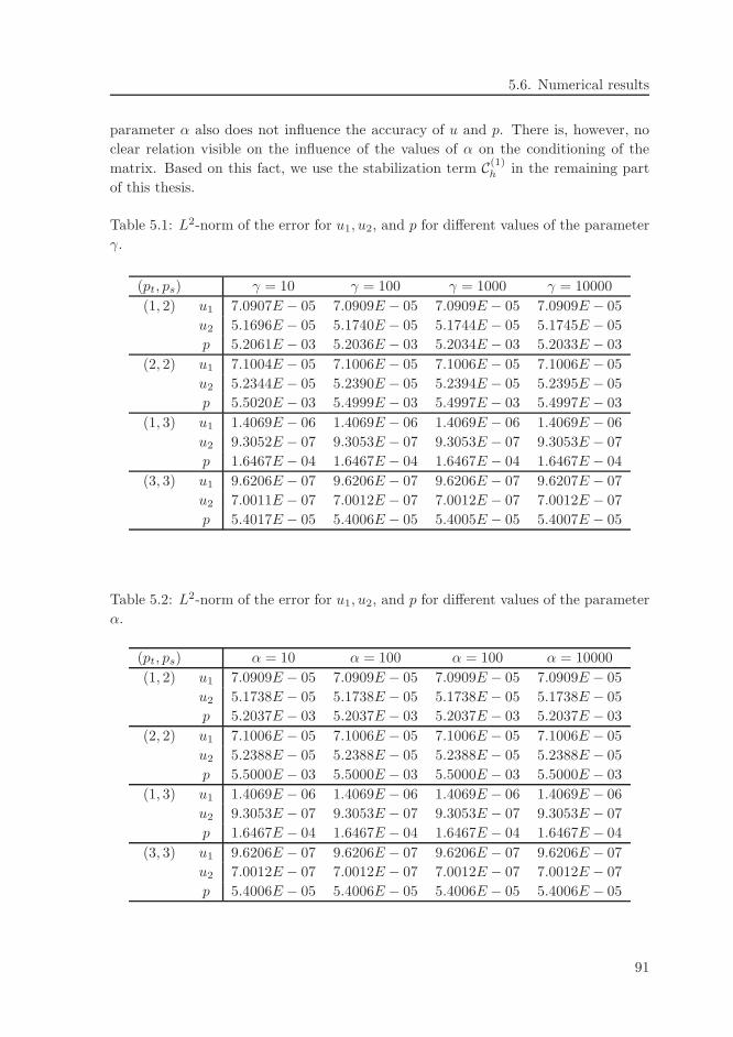
5.6. Numerical results
parameter α also does not influence the accuracy of u and p. There is, however, no
clear relation visible on the influence of the values of α on the conditioning of the
matrix. Based on this fact, we use the stabilization term C(1)h in the remaining part
of this thesis.
Table 5.1: L2-norm of the error for u1, u2, and p for different values of the parameter
γ.
(pt, ps) γ = 10 γ = 100 γ = 1000 γ = 10000
(1, 2) u1 7.0907E − 05 7.0909E − 05 7.0909E − 05 7.0909E − 05
u2 5.1696E − 05 5.1740E − 05 5.1744E − 05 5.1745E − 05
p 5.2061E − 03 5.2036E − 03 5.2034E − 03 5.2033E − 03
(2, 2) u1 7.1004E − 05 7.1006E − 05 7.1006E − 05 7.1006E − 05
u2 5.2344E − 05 5.2390E − 05 5.2394E − 05 5.2395E − 05
p 5.5020E − 03 5.4999E − 03 5.4997E − 03 5.4997E − 03
(1, 3) u1 1.4069E − 06 1.4069E − 06 1.4069E − 06 1.4069E − 06
u2 9.3052E − 07 9.3053E − 07 9.3053E − 07 9.3053E − 07
p 1.6467E − 04 1.6467E − 04 1.6467E − 04 1.6467E − 04
(3, 3) u1 9.6206E − 07 9.6206E − 07 9.6206E − 07 9.6207E − 07
u2 7.0011E − 07 7.0012E − 07 7.0012E − 07 7.0012E − 07
p 5.4017E − 05 5.4006E − 05 5.4005E − 05 5.4007E − 05
Table 5.2: L2-norm of the error for u1, u2, and p for different values of the parameter
α.
(pt, ps) α = 10 α = 100 α = 100 α = 10000
(1, 2) u1 7.0909E − 05 7.0909E − 05 7.0909E − 05 7.0909E − 05
u2 5.1738E − 05 5.1738E − 05 5.1738E − 05 5.1738E − 05
p 5.2037E − 03 5.2037E − 03 5.2037E − 03 5.2037E − 03
(2, 2) u1 7.1006E − 05 7.1006E − 05 7.1006E − 05 7.1006E − 05
u2 5.2388E − 05 5.2388E − 05 5.2388E − 05 5.2388E − 05
p 5.5000E − 03 5.5000E − 03 5.5000E − 03 5.5000E − 03
(1, 3) u1 1.4069E − 06 1.4069E − 06 1.4069E − 06 1.4069E − 06
u2 9.3053E − 07 9.3053E − 07 9.3053E − 07 9.3053E − 07
p 1.6467E − 04 1.6467E − 04 1.6467E − 04 1.6467E − 04
(3, 3) u1 9.6206E − 07 9.6206E − 07 9.6206E − 07 9.6206E − 07
u2 7.0012E − 07 7.0012E − 07 7.0012E − 07 7.0012E − 07
p 5.4006E − 05 5.4006E − 05 5.4006E − 05 5.4006E − 05
91
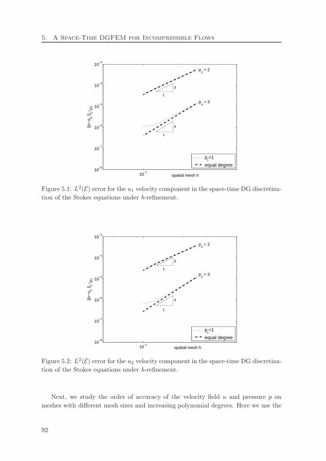
5. A Space-Time DGFEM for Incompressible Flows
10−1
10−8
10−7
10−6
10−5
10−4
10−3
spatial mesh h
||u−
u h ||L2 (E
)
ps = 2
ps = 3
1
1
3
4
pt=1
equal degree
Figure 5.1: L2(E) error for the u1 velocity component in the space-time DG discretiza-
tion of the Stokes equations under h-refinement.
10−1
10−8
10−7
10−6
10−5
10−4
10−3
spatial mesh h
||u−
u h ||L2 (E
)
ps = 2
ps = 3
1
1
3
4
pt=1
equal degree
Figure 5.2: L2(E) error for the u2 velocity component in the space-time DG discretiza-
tion of the Stokes equations under h-refinement.
Next, we study the order of accuracy of the velocity field u and pressure p on
meshes with different mesh sizes and increasing polynomial degrees. Here we use the
92
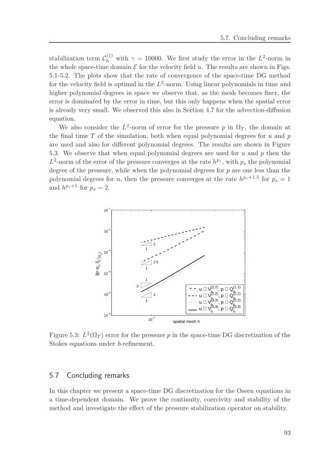
5.7. Concluding remarks
stabilization term C(1)h with γ = 10000. We first study the error in the L2-norm in
the whole space-time domain E for the velocity field u. The results are shown in Figs.
5.1-5.2. The plots show that the rate of convergence of the space-time DG method
for the velocity field is optimal in the L2-norm. Using linear polynomials in time and
higher polynomial degrees in space we observe that, as the mesh becomes finer, the
error is dominated by the error in time, but this only happens when the spatial error
is already very small. We observed this also in Section 4.7 for the advection-diffusion
equation.
We also consider the L2-norm of error for the pressure p in ΩT , the domain at
the final time T of the simulation, both when equal polynomial degrees for u and p
are used and also for different polynomial degrees. The results are shown in Figure
5.3. We observe that when equal polynomial degrees are used for u and p then the
L2-norm of the error of the pressure converges at the rate hps , with ps the polynomial
degree of the pressure, while when the polynomial degrees for p are one less than the
polynomial degrees for u, then the pressure converges at the rate hps+1.5 for ps = 1
and hps+1 for ps = 2.
10−1
10−6
10−5
10−4
10−3
10−2
10−1
spatial mesh h
||p−
p h ||L2 (Ω
T)
1
1
1
1
2
2.5
3
3
u ∈ Vh(2,2), p ∈ Q
h(1,1)
u ∈ Vh(2,2), p ∈ Q
h(2,2)
u ∈ Vh(3,3), p ∈ Q
h(2,2)
u ∈ Vh(3,3), p ∈ Q
h(3,3)
Figure 5.3: L2(ΩT ) error for the pressure p in the space-time DG discretization of the
Stokes equations under h-refinement.
5.7 Concluding remarks
In this chapter we present a space-time DG discretization for the Oseen equations in
a time-dependent domain. We prove the continuity, coercivity and stability of the
method and investigate the effect of the pressure stabilization operator on stability.
93
5. A Space-Time DGFEM for Incompressible Flows
The simulations show that the values of the parameter γ in the pressure stabi-
lization operator C(1)h do not influence the accuracy of the method. The values of γ
have, however, a significant effect on the conditioning of the matrix resulting from the
discretization. Larger values of γ give a better conditioning of the matrix. The values
of the parameter α in the pressure stabilization operator C(2)h also does not influence
the accuracy. Unfortunately, no conclusion can be obtained on the effect of α on the
conditioning of the matrix.
The numerical experiments show that the convergence rate of the space-time DG
solution for the velocity field is optimal in the L2-norm, while the pressure converges
at the rate hps for equal polynomial degrees of the velocity and pressure, with ps
the polynomial degree of the pressure, and between hps+1 and hps+1.5 for mixed
polynomial degrees. The simulations show that the algorithm also performs well for
higher polynomial degrees in time.
The space-time DG discretization in this chapter is limited to the Oseen equations,
the extension to the incompressible Navier-Stokes equations which requires the use
of a projection operator to ensure a divergence free velocity field will be discussed in
[62].
94
Chapter 6
Simulation of Wet-Chemical Etching Processes
6.1 Introduction
In this chapter we present simulation results for different types of wet-chemical etching
processes. The equations describing the transport phenomena in wet-chemical etching
have been stated in Chapter 2, and consist of an advection-diffusion equation for the
etchant concentration, the incompressible Navier-Stokes equations to model the flow
of the etchant, and an equation for the movement of the etching surface.
A space-time DG discretization for the advection-diffusion equation has been de-
veloped in Chapter 4, while in Chapter 5 a space-time DG discretization for the
incompressible Navier-Stokes equations has been worked out. In this chapter we
will first discuss in Section 6.2 the DG discretization of the equation for the moving
boundary of the etching surface. Next, a special technique to construct an initial
space-time computational mesh is described in Section 6.3. These algorithms will be
used to discretize the equations describing wet-chemical etching processes.
In the second part of this chapter simulation results using DG discretizations for
different types of wet-chemical etching processes will be discussed. Part of these
results have been presented in [60].
6.2 Discretization of the equation for the moving boundary
First, we recall the dimensionless form of the moving boundary equation (2.11) for
each Cartesian component xs,i of a point xs at the cavity surface:
dxs,i
dt= − 1
βni
d∑
j=1
∂c
∂xjnj , j = 1, . . . , d. (6.1)
We consider the movement of the etching surface in a time interval In = (tn, tn+1).
For each time interval we assume that In is an image of a reference interval I = (−1, 1)
95
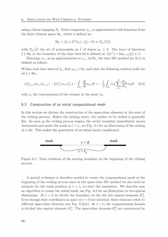
6. Simulation of Wet-Chemical Etching
using a linear mapping FI . Each component xs,i is approximated with functions from
the finite element space Θh, which is defined as:
Θh = ξ ∈ L2(In) : ξ|I FI ∈ PpI(I),
with PpI(I) the set of polynomials on I of degree pI ≥ 0. The trace of functions
ξ ∈ Θh at the boundary of the time interval is defined as: ξ(t±) = limǫ→0 ξ(t± ǫ).Denoting xh,i as an approximation to xs,i in Θh, the time DG method for (6.1) is
defined as follows:
Within each time interval In, find xh,i ∈ Θh such that the following relation holds for
all ξ ∈ Θh:
ξ(t−n+1)xh,i(t−n+1)− ξ(t+n )xh,i(t
−n )−
∫
In
dξ
dtxh,idt = − 1
β
∫
In
niξ
d∑
j=1
∂cs∂xj
njdt, (6.2)
with cs the concentration of the etchant at the point xh.
6.3 Construction of an initial computational mesh
In this section we discuss the construction of the space-time elements at the start of
the etching process. Before the etching starts, the surface to be etched is generally
flat. As soon as the etching process begins, the cavity boundary immediately moves
downwards and under the mask at t = t1, see Fig. 6.1 for an illustration of the etching
of a slit. This makes the generation of an initial mesh complicated.
mask maskt = 0
t = t1
Figure 6.1: Time evolution of the moving boundary at the beginning of the etching
process.
A special technique is therefore needed to create the computational mesh at the
beginning of the etching process since in the space-time DG method we also need an
estimate for the mesh position at t = t1 to start the simulation. We describe now
an algorithm to create the initial mesh, see Fig. 6.2 for an illustration in two-spatial
dimensions. At t = 0 we divide the boundary on the slit into spatial elements K0j .
Even though their coordinates in space at t = 0 are identical, these elements relate to
different space-time elements (see Fig. 6.2(a)). At t = t1 the computational domain
is divided into spatial elements K1j . The space-time elements K0
j are constructed by
96
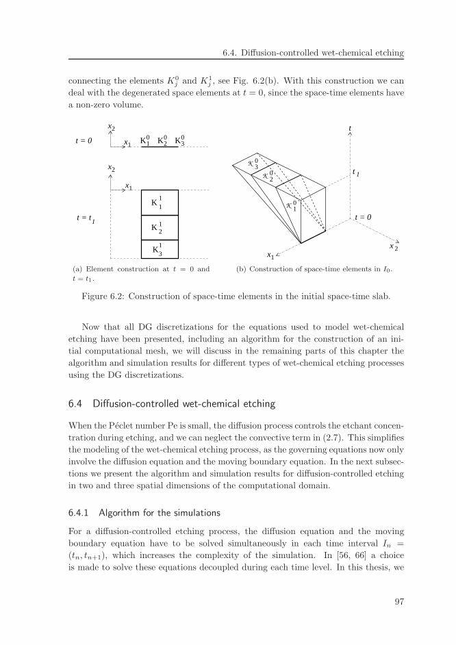
6.4. Diffusion-controlled wet-chemical etching
connecting the elements K0j and K1
j , see Fig. 6.2(b). With this construction we can
deal with the degenerated space elements at t = 0, since the space-time elements have
a non-zero volume.
x
xt = 0
t = t1
K K K0 0 01 2 3
K
K
K
1
2
31
1
1
x
x
1
1
2
2
(a) Element construction at t = 0 and
t = t1.
t 1
t
x
t = 0
K
K
K1
0
0
2
30
x1
2
(b) Construction of space-time elements in I0.
Figure 6.2: Construction of space-time elements in the initial space-time slab.
Now that all DG discretizations for the equations used to model wet-chemical
etching have been presented, including an algorithm for the construction of an ini-
tial computational mesh, we will discuss in the remaining parts of this chapter the
algorithm and simulation results for different types of wet-chemical etching processes
using the DG discretizations.
6.4 Diffusion-controlled wet-chemical etching
When the Peclet number Pe is small, the diffusion process controls the etchant concen-
tration during etching, and we can neglect the convective term in (2.7). This simplifies
the modeling of the wet-chemical etching process, as the governing equations now only
involve the diffusion equation and the moving boundary equation. In the next subsec-
tions we present the algorithm and simulation results for diffusion-controlled etching
in two and three spatial dimensions of the computational domain.
6.4.1 Algorithm for the simulations
For a diffusion-controlled etching process, the diffusion equation and the moving
boundary equation have to be solved simultaneously in each time interval In =
(tn, tn+1), which increases the complexity of the simulation. In [56, 66] a choice
is made to solve these equations decoupled during each time level. In this thesis, we
97
6. Simulation of Wet-Chemical Etching
solve both equations simultaneously by conducting an iteration process. First, the
moving boundary equation is solved to obtain the new position of the etching surface.
The initial concentration used in the moving boundary equation is the one computed
in the previous time step. Then, the diffusion equation is solved in the computational
domain with the updated boundary position, which also provides a new concentra-
tion for the moving boundary equation. This iteration process is continued until the
position of the etching surface at the new time level is obtained. The main steps in
simulating diffusion-controlled wet-chemical etching are summarized in the following
algorithm.
Algorithm 6.1 Algorithm for simulating diffusion-controlled wet-chemical etching.
(1) At the start of the computation in the time interval In, set c(0)h = cn and
x(0)s = xn
s , the concentration and the cavity surface points, respectively, from
the previous time interval.
(2) Set the maximum iteration count maxit and stopping criterion ǫ.
(3) Do for each iteration i = 1, 2, . . . ,maxit:
(i) For all points x(i−1)s,j , j = 1, . . . , Ns, with Ns the number of points at the
etching surface:
Solve (6.2) with cs = c(i−1)h for each Cartesian component of the etching
surface points to obtain x(i)s,j .
(ii) Compute the maximum in the change of the boundary position:
x(i)s,max = max
j|x(i)
s,j − x(i−1)s,j |,
and compute the ratio r(i)s = |x(i)
s,max − x(i−1)s,max|/x(i)
s,max.
(iii) Move the coordinates of the etching surface to the new position x(i)s .
(iv) If r(i)s < ǫ, stop the iteration. If not, continue the iteration procedure.
(v) Solve (2.7) in the new coordinates to obtain c(i)h .
(4) The position of the etching surface at tn+1 is now equal to xn+1s .
(5) Update the mesh and refine the elements if the mesh becomes too coarse due
to the boundary movement.
(6) Solve (2.7) with the new coordinates xn+1s to obtain cn+1
h , the space-time DG
solution of the etchant concentration in the time interval In.
98
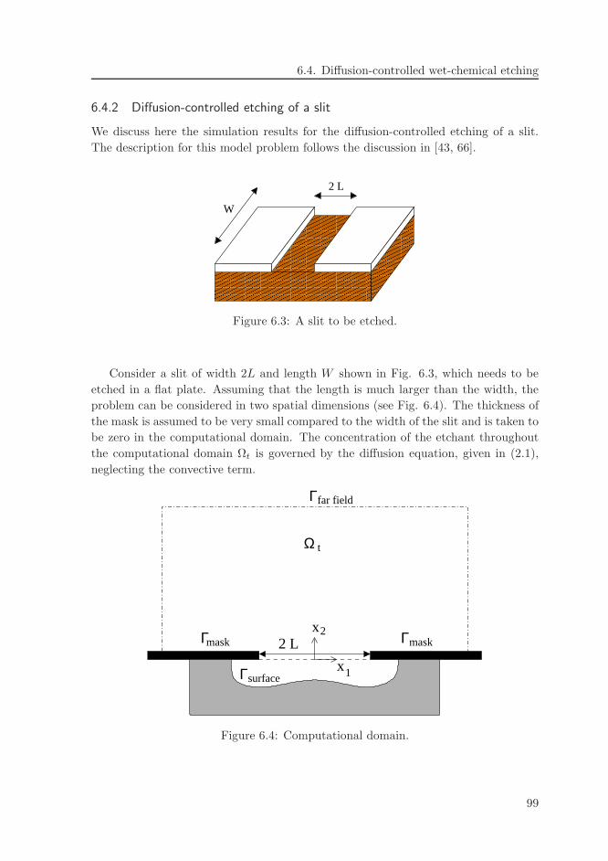
6.4. Diffusion-controlled wet-chemical etching
6.4.2 Diffusion-controlled etching of a slit
We discuss here the simulation results for the diffusion-controlled etching of a slit.
The description for this model problem follows the discussion in [43, 66].
W
2 L
Figure 6.3: A slit to be etched.
Consider a slit of width 2L and length W shown in Fig. 6.3, which needs to be
etched in a flat plate. Assuming that the length is much larger than the width, the
problem can be considered in two spatial dimensions (see Fig. 6.4). The thickness of
the mask is assumed to be very small compared to the width of the slit and is taken to
be zero in the computational domain. The concentration of the etchant throughout
the computational domain Ωt is governed by the diffusion equation, given in (2.1),
neglecting the convective term.
Γ
Γmask
far field
Γsurface
maskΓ
tΩ
2 Lx2
x1
Figure 6.4: Computational domain.
99
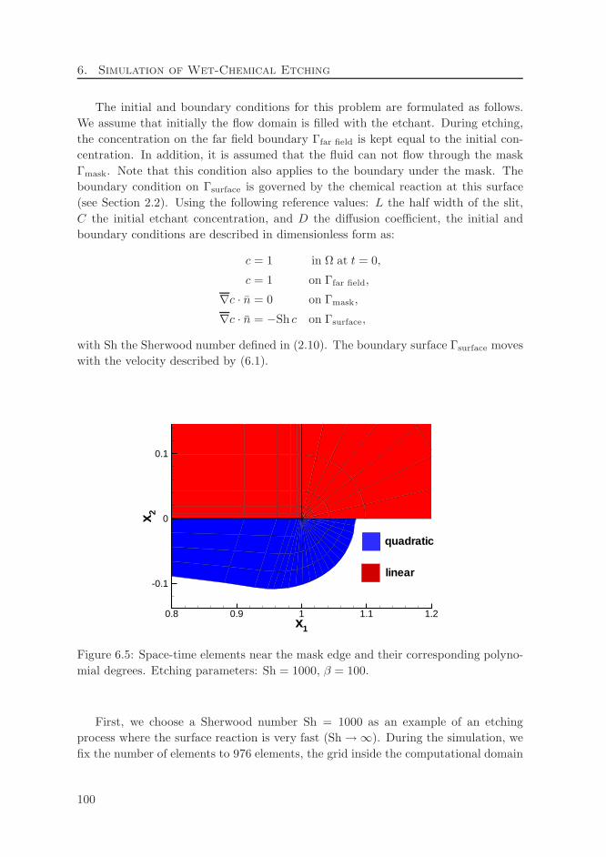
6. Simulation of Wet-Chemical Etching
The initial and boundary conditions for this problem are formulated as follows.
We assume that initially the flow domain is filled with the etchant. During etching,
the concentration on the far field boundary Γfar field is kept equal to the initial con-
centration. In addition, it is assumed that the fluid can not flow through the mask
Γmask. Note that this condition also applies to the boundary under the mask. The
boundary condition on Γsurface is governed by the chemical reaction at this surface
(see Section 2.2). Using the following reference values: L the half width of the slit,
C the initial etchant concentration, and D the diffusion coefficient, the initial and
boundary conditions are described in dimensionless form as:
c = 1 in Ω at t = 0,
c = 1 on Γfar field,
∇c · n = 0 on Γmask,
∇c · n = −Sh c on Γsurface,
with Sh the Sherwood number defined in (2.10). The boundary surface Γsurface moves
with the velocity described by (6.1).
x1
x 2
0.8 0.9 1 1.1 1.2
-0.1
0
0.1
quadratic
linear
Figure 6.5: Space-time elements near the mask edge and their corresponding polyno-
mial degrees. Etching parameters: Sh = 1000, β = 100.
First, we choose a Sherwood number Sh = 1000 as an example of an etching
process where the surface reaction is very fast (Sh→∞). During the simulation, we
fix the number of elements to 976 elements, the grid inside the computational domain
100
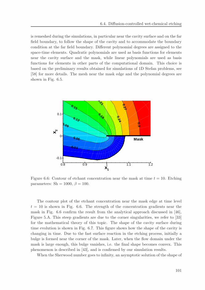
6.4. Diffusion-controlled wet-chemical etching
is remeshed during the simulations, in particular near the cavity surface and on the far
field boundary, to follow the shape of the cavity and to accommodate the boundary
condition at the far field boundary. Different polynomial degrees are assigned to the
space-time elements. Quadratic polynomials are used as basis functions for elements
near the cavity surface and the mask, while linear polynomials are used as basis
functions for elements in other parts of the computational domain. This choice is
based on the preliminary results obtained for simulations of 1D Stefan problems, see
[58] for more details. The mesh near the mask edge and the polynomial degrees are
shown in Fig. 6.5.
0.03
0.06
0.09
0.12
0.15
0.18
0.21
0.240.27
0.3
x1
x 2
0.8 0.9 1 1.1 1.2
-0.1
0
0.1
Mask
Figure 6.6: Contour of etchant concentration near the mask at time t = 10. Etching
parameters: Sh = 1000, β = 100.
The contour plot of the etchant concentration near the mask edge at time level
t = 10 is shown in Fig. 6.6. The strength of the concentration gradients near the
mask in Fig. 6.6 confirm the result from the analytical approach discussed in [46],
Figure 5.A. This steep gradients are due to the corner singularities, we refer to [33]
for the mathematical theory of this topic. The shape of the cavity surface during
time evolution is shown in Fig. 6.7. This figure shows how the shape of the cavity is
changing in time. Due to the fast surface reaction in the etching process, initially a
bulge is formed near the corner of the mask. Later, when the flow domain under the
mask is large enough, this bulge vanishes, i.e. the final shape becomes convex. This
phenomenon is described in [43], and is confirmed by our simulation results.
When the Sherwood number goes to infinity, an asymptotic solution of the shape of
101
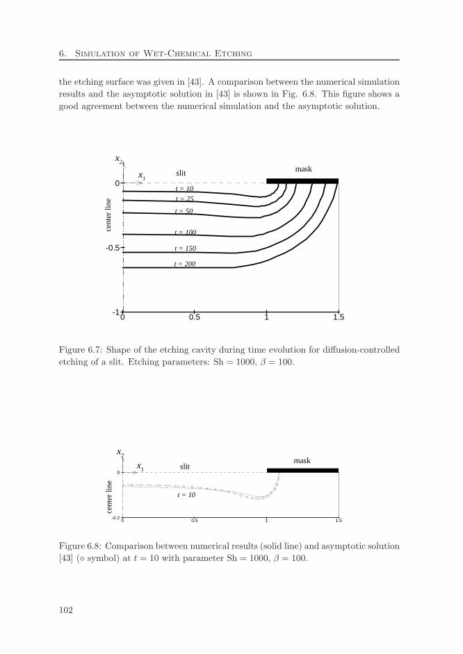
6. Simulation of Wet-Chemical Etching
the etching surface was given in [43]. A comparison between the numerical simulation
results and the asymptotic solution in [43] is shown in Fig. 6.8. This figure shows a
good agreement between the numerical simulation and the asymptotic solution.
0 0.5 1 1.5-1
-0.5
0
t = 50
x1
t = 150
t = 25
t = 100
t = 10
t = 200
slit
cent
erlin
e
maskx2
Figure 6.7: Shape of the etching cavity during time evolution for diffusion-controlled
etching of a slit. Etching parameters: Sh = 1000, β = 100.
0 0.5 1 1.5-0.2
0x1
t = 10
slit
cent
erlin
e
maskx2
Figure 6.8: Comparison between numerical results (solid line) and asymptotic solution
[43] (⋄ symbol) at t = 10 with parameter Sh = 1000, β = 100.
102
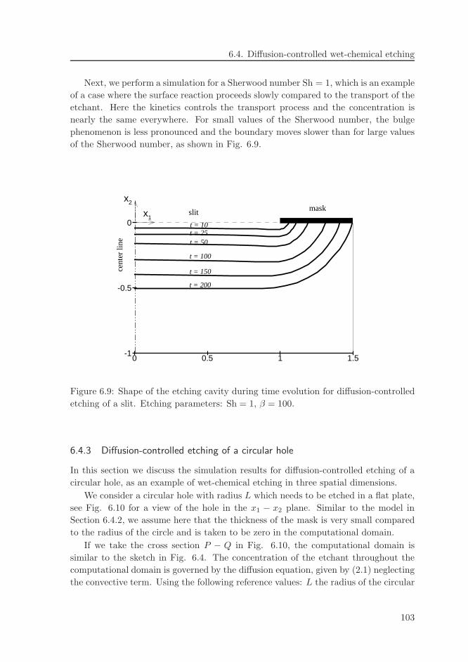
6.4. Diffusion-controlled wet-chemical etching
Next, we perform a simulation for a Sherwood number Sh = 1, which is an example
of a case where the surface reaction proceeds slowly compared to the transport of the
etchant. Here the kinetics controls the transport process and the concentration is
nearly the same everywhere. For small values of the Sherwood number, the bulge
phenomenon is less pronounced and the boundary moves slower than for large values
of the Sherwood number, as shown in Fig. 6.9.
0 0.5 1 1.5-1
-0.5
0
t = 50
x1
t = 150
t = 25
t = 100
t = 10
t = 200
slit
cent
erlin
e
maskx2
Figure 6.9: Shape of the etching cavity during time evolution for diffusion-controlled
etching of a slit. Etching parameters: Sh = 1, β = 100.
6.4.3 Diffusion-controlled etching of a circular hole
In this section we discuss the simulation results for diffusion-controlled etching of a
circular hole, as an example of wet-chemical etching in three spatial dimensions.
We consider a circular hole with radius L which needs to be etched in a flat plate,
see Fig. 6.10 for a view of the hole in the x1 − x2 plane. Similar to the model in
Section 6.4.2, we assume here that the thickness of the mask is very small compared
to the radius of the circle and is taken to be zero in the computational domain.
If we take the cross section P − Q in Fig. 6.10, the computational domain is
similar to the sketch in Fig. 6.4. The concentration of the etchant throughout the
computational domain is governed by the diffusion equation, given by (2.1) neglecting
the convective term. Using the following reference values: L the radius of the circular
103
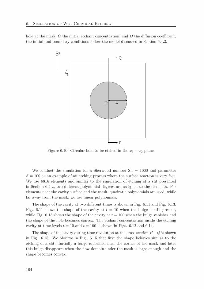
6. Simulation of Wet-Chemical Etching
hole at the mask, C the initial etchant concentration, and D the diffusion coefficient,
the initial and boundary conditions follow the model discussed in Section 6.4.2.
L
P
x
x1
Q2
O
Figure 6.10: Circular hole to be etched in the x1 − x2 plane.
We conduct the simulation for a Sherwood number Sh = 1000 and parameter
β = 100 as an example of an etching process where the surface reaction is very fast.
We use 6816 elements and similar to the simulation of etching of a slit presented
in Section 6.4.2, two different polynomial degrees are assigned to the elements. For
elements near the cavity surface and the mask, quadratic polynomials are used, while
far away from the mask, we use linear polynomials.
The shape of the cavity at two different times is shown in Fig. 6.11 and Fig. 6.13.
Fig. 6.11 shows the shape of the cavity at t = 10 when the bulge is still present,
while Fig. 6.13 shows the shape of the cavity at t = 100 when the bulge vanishes and
the shape of the hole becomes convex. The etchant concentration inside the etching
cavity at time levels t = 10 and t = 100 is shown in Figs. 6.12 and 6.14.
The shape of the cavity during time revolution at the cross section P −Q is shown
in Fig. 6.15. We observe in Fig. 6.15 that first the shape behaves similar to the
etching of a slit. Initially a bulge is formed near the corner of the mask and later
this bulge disappears when the flow domain under the mask is large enough and the
shape becomes convex.
104
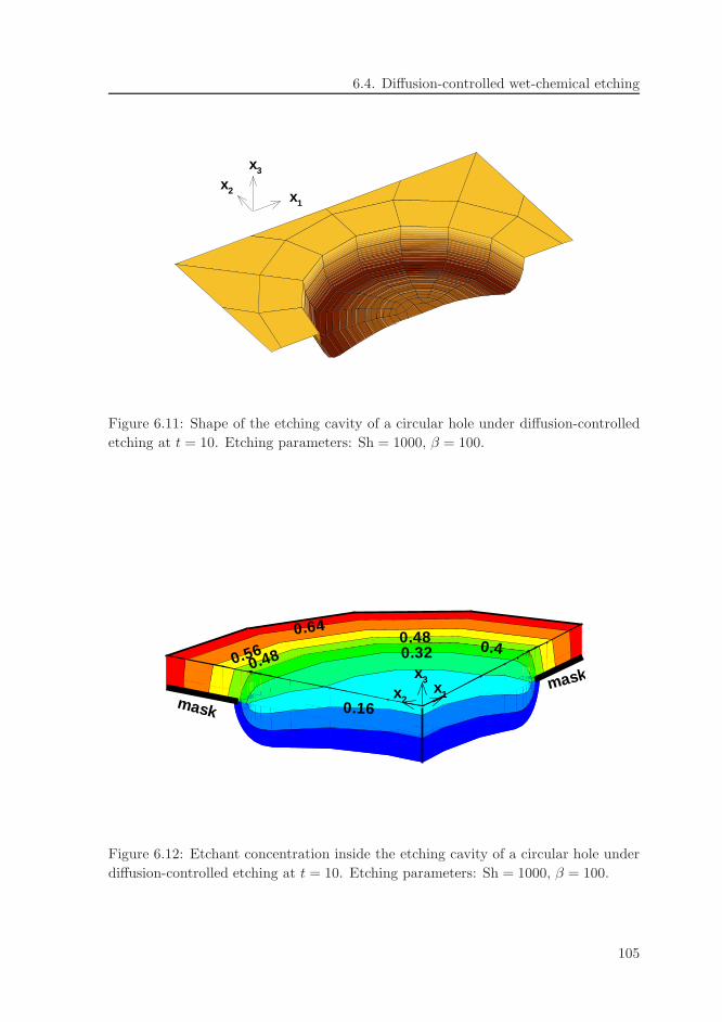
6.4. Diffusion-controlled wet-chemical etching
x3
x2 x1
Figure 6.11: Shape of the etching cavity of a circular hole under diffusion-controlled
etching at t = 10. Etching parameters: Sh = 1000, β = 100.
0.16
0.40.480.56
0.64
0.320.48
mask
maskx3x1x2
Figure 6.12: Etchant concentration inside the etching cavity of a circular hole under
diffusion-controlled etching at t = 10. Etching parameters: Sh = 1000, β = 100.
105
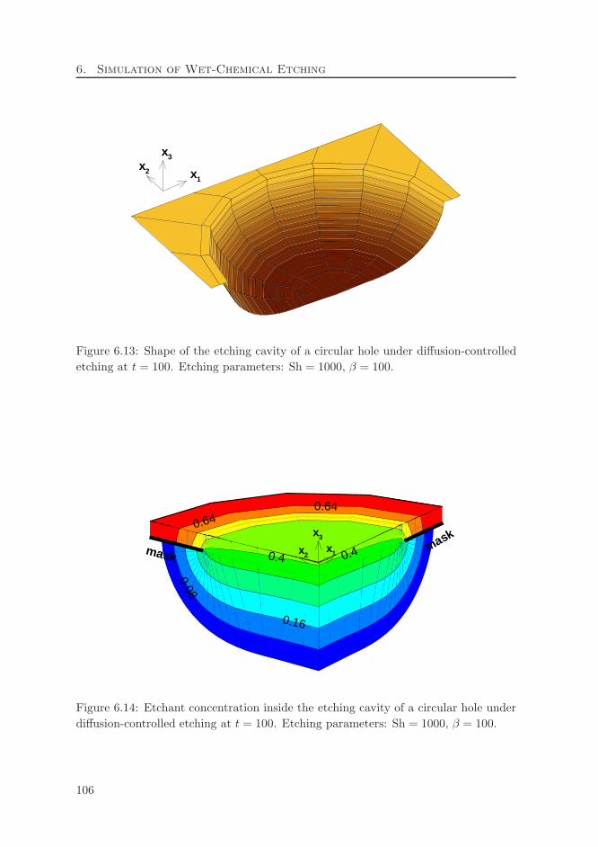
6. Simulation of Wet-Chemical Etching
x3
x1
x2
Figure 6.13: Shape of the etching cavity of a circular hole under diffusion-controlled
etching at t = 100. Etching parameters: Sh = 1000, β = 100.
0.16
0.08
0.40.4
0.64
0.64
maskmaskx3
x2x1
Figure 6.14: Etchant concentration inside the etching cavity of a circular hole under
diffusion-controlled etching at t = 100. Etching parameters: Sh = 1000, β = 100.
106
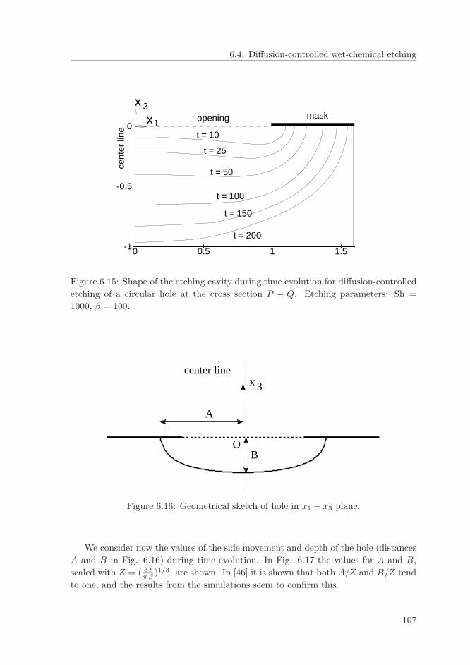
6.4. Diffusion-controlled wet-chemical etching
0 0.5 1 1.5-1
-0.5
0maskx
x
1
3
t = 10
t = 25
t = 50
t = 100
t = 150
t = 200
openingce
nter
line
Figure 6.15: Shape of the etching cavity during time evolution for diffusion-controlled
etching of a circular hole at the cross section P − Q. Etching parameters: Sh =
1000, β = 100.
center linex 3
A
BO
Figure 6.16: Geometrical sketch of hole in x1 − x3 plane.
We consider now the values of the side movement and depth of the hole (distances
A and B in Fig. 6.16) during time evolution. In Fig. 6.17 the values for A and B,
scaled with Z = ( 3 tπ β )1/3, are shown. In [46] it is shown that both A/Z and B/Z tend
to one, and the results from the simulations seem to confirm this.
107
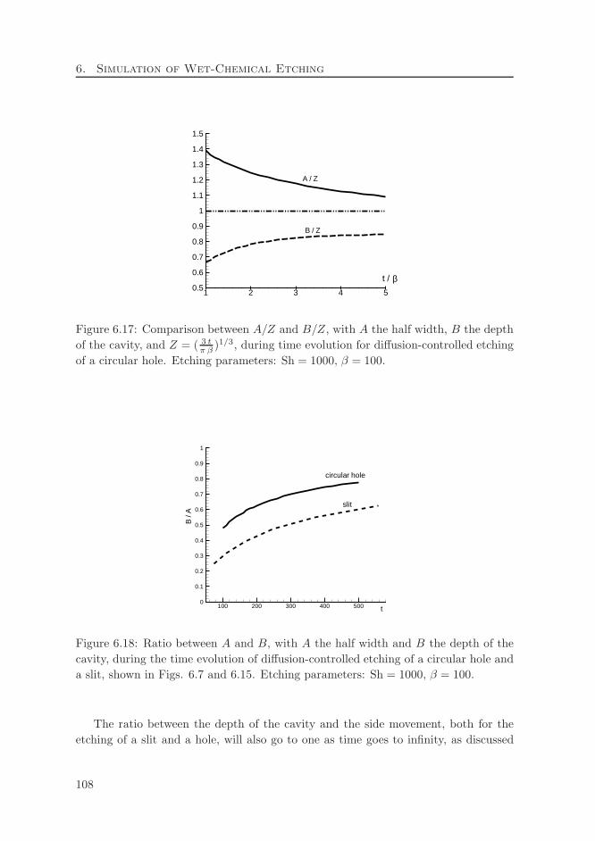
6. Simulation of Wet-Chemical Etching
1 2 3 4 50.5
0.6
0.7
0.8
0.9
1
1.1
1.2
1.3
1.4
1.5
B / Z
A / Z
t / β
Figure 6.17: Comparison between A/Z and B/Z, with A the half width, B the depth
of the cavity, and Z = ( 3 tπ β )1/3, during time evolution for diffusion-controlled etching
of a circular hole. Etching parameters: Sh = 1000, β = 100.
100 200 300 400 5000
0.1
0.2
0.3
0.4
0.5
0.6
0.7
0.8
0.9
1
t
B/A
circular hole
slit
Figure 6.18: Ratio between A and B, with A the half width and B the depth of the
cavity, during the time evolution of diffusion-controlled etching of a circular hole and
a slit, shown in Figs. 6.7 and 6.15. Etching parameters: Sh = 1000, β = 100.
The ratio between the depth of the cavity and the side movement, both for the
etching of a slit and a hole, will also go to one as time goes to infinity, as discussed
108
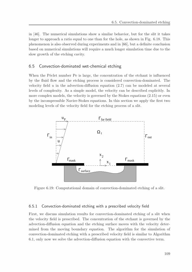
6.5. Convection-dominated etching
in [46]. The numerical simulations show a similar behavior, but for the slit it takes
longer to approach a ratio equal to one than for the hole, as shown in Fig. 6.18. This
phenomenon is also observed during experiments and in [66], but a definite conclusion
based on numerical simulations will require a much longer simulation time due to the
slow growth of the etching cavity.
6.5 Convection-dominated wet-chemical etching
When the Peclet number Pe is large, the concentration of the etchant is influenced
by the fluid flow and the etching process is considered convection-dominated. The
velocity field u in the advection-diffusion equation (2.7) can be modeled at several
levels of complexity. As a simple model, the velocity can be described explicitly. In
more complex models, the velocity is governed by the Stokes equations (2.15) or even
by the incompressible Navier-Stokes equations. In this section we apply the first two
modeling levels of the velocity field for the etching process of a slit.
Γ
Γmask
far field
Γsurface
maskΓ
tΩΓ Γin out
u
x2
1x
Fu
Figure 6.19: Computational domain of convection-dominated etching of a slit.
6.5.1 Convection-dominated etching with a prescribed velocity field
First, we discuss simulation results for convection-dominated etching of a slit when
the velocity field is prescribed. The concentration of the etchant is governed by the
advection-diffusion equation and the etching surface moves with the velocity deter-
mined from the moving boundary equation. The algorithm for the simulation of
convection-dominated etching with a prescribed velocity field is similar to Algorithm
6.1, only now we solve the advection-diffusion equation with the convective term.
109
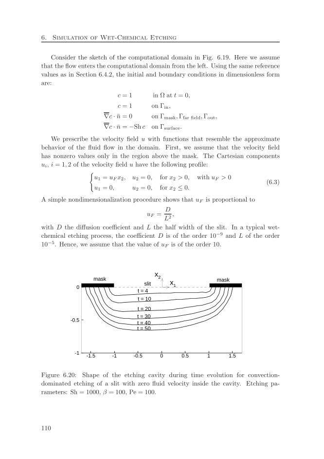
6. Simulation of Wet-Chemical Etching
Consider the sketch of the computational domain in Fig. 6.19. Here we assume
that the flow enters the computational domain from the left. Using the same reference
values as in Section 6.4.2, the initial and boundary conditions in dimensionless form
are:
c = 1 in Ω at t = 0,
c = 1 on Γin,
∇c · n = 0 on Γmask,Γfar field,Γout,
∇c · n = −Sh c on Γsurface.
We prescribe the velocity field u with functions that resemble the approximate
behavior of the fluid flow in the domain. First, we assume that the velocity field
has nonzero values only in the region above the mask. The Cartesian components
ui, i = 1, 2 of the velocity field u have the following profile:
u1 = uFx2, u2 = 0, for x2 > 0, with uF > 0
u1 = 0, u2 = 0, for x2 ≤ 0.(6.3)
A simple nondimensionalization procedure shows that uF is proportional to
uF =D
L2,
with D the diffusion coefficient and L the half width of the slit. In a typical wet-
chemical etching process, the coefficient D is of the order 10−9 and L of the order
10−5. Hence, we assume that the value of uF is of the order 10.
-1.5 -1 -0.5 0 0.5 1 1.5-1
-0.5
0x1
x2mask maskslit
t = 4
t = 10
t = 20t = 30t = 40t = 50
Figure 6.20: Shape of the etching cavity during time evolution for convection-
dominated etching of a slit with zero fluid velocity inside the cavity. Etching pa-
rameters: Sh = 1000, β = 100, Pe = 100.
110
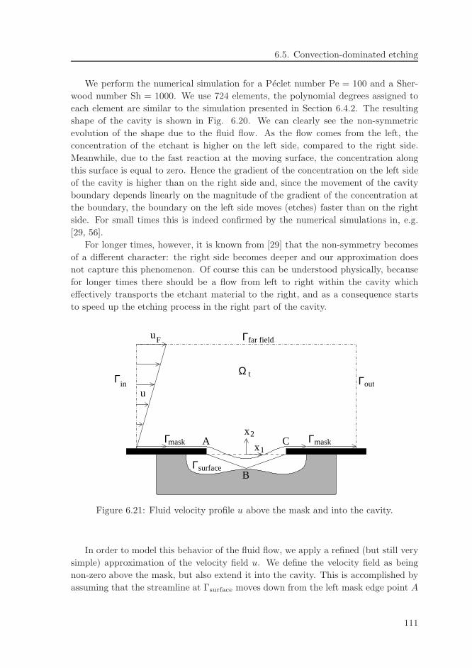
6.5. Convection-dominated etching
We perform the numerical simulation for a Peclet number Pe = 100 and a Sher-
wood number Sh = 1000. We use 724 elements, the polynomial degrees assigned to
each element are similar to the simulation presented in Section 6.4.2. The resulting
shape of the cavity is shown in Fig. 6.20. We can clearly see the non-symmetric
evolution of the shape due to the fluid flow. As the flow comes from the left, the
concentration of the etchant is higher on the left side, compared to the right side.
Meanwhile, due to the fast reaction at the moving surface, the concentration along
this surface is equal to zero. Hence the gradient of the concentration on the left side
of the cavity is higher than on the right side and, since the movement of the cavity
boundary depends linearly on the magnitude of the gradient of the concentration at
the boundary, the boundary on the left side moves (etches) faster than on the right
side. For small times this is indeed confirmed by the numerical simulations in, e.g.
[29, 56].
For longer times, however, it is known from [29] that the non-symmetry becomes
of a different character: the right side becomes deeper and our approximation does
not capture this phenomenon. Of course this can be understood physically, because
for longer times there should be a flow from left to right within the cavity which
effectively transports the etchant material to the right, and as a consequence starts
to speed up the etching process in the right part of the cavity.
Γ
Γmask
far field
Γsurface
maskΓ
tΩΓ Γin out
u
B
CAx1
x2
uF
Figure 6.21: Fluid velocity profile u above the mask and into the cavity.
In order to model this behavior of the fluid flow, we apply a refined (but still very
simple) approximation of the velocity field u. We define the velocity field as being
non-zero above the mask, but also extend it into the cavity. This is accomplished by
assuming that the streamline at Γsurface moves down from the left mask edge point A
111
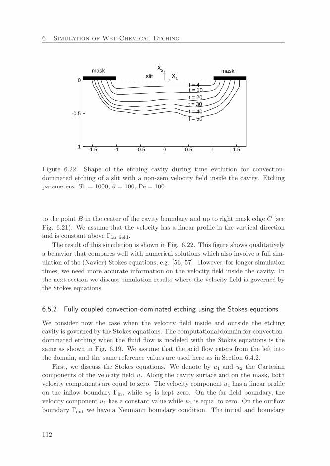
6. Simulation of Wet-Chemical Etching
-1.5 -1 -0.5 0 0.5 1 1.5-1
-0.5
0x1
x2mask maskslit
t = 4t = 10t = 20t = 30t = 40t = 50
Figure 6.22: Shape of the etching cavity during time evolution for convection-
dominated etching of a slit with a non-zero velocity field inside the cavity. Etching
parameters: Sh = 1000, β = 100, Pe = 100.
to the point B in the center of the cavity boundary and up to right mask edge C (see
Fig. 6.21). We assume that the velocity has a linear profile in the vertical direction
and is constant above Γfar field.
The result of this simulation is shown in Fig. 6.22. This figure shows qualitatively
a behavior that compares well with numerical solutions which also involve a full sim-
ulation of the (Navier)-Stokes equations, e.g. [56, 57]. However, for longer simulation
times, we need more accurate information on the velocity field inside the cavity. In
the next section we discuss simulation results where the velocity field is governed by
the Stokes equations.
6.5.2 Fully coupled convection-dominated etching using the Stokes equations
We consider now the case when the velocity field inside and outside the etching
cavity is governed by the Stokes equations. The computational domain for convection-
dominated etching when the fluid flow is modeled with the Stokes equations is the
same as shown in Fig. 6.19. We assume that the acid flow enters from the left into
the domain, and the same reference values are used here as in Section 6.4.2.
First, we discuss the Stokes equations. We denote by u1 and u2 the Cartesian
components of the velocity field u. Along the cavity surface and on the mask, both
velocity components are equal to zero. The velocity component u1 has a linear profile
on the inflow boundary Γin, while u2 is kept zero. On the far field boundary, the
velocity component u1 has a constant value while u2 is equal to zero. On the outflow
boundary Γout we have a Neumann boundary condition. The initial and boundary
112
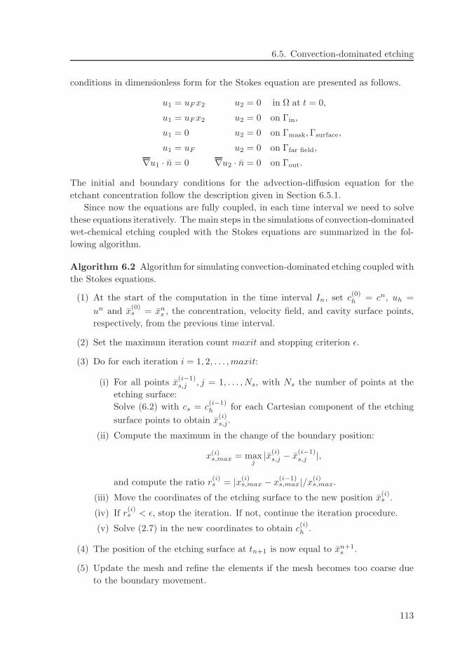
6.5. Convection-dominated etching
conditions in dimensionless form for the Stokes equation are presented as follows.
u1 = uFx2 u2 = 0 in Ω at t = 0,
u1 = uFx2 u2 = 0 on Γin,
u1 = 0 u2 = 0 on Γmask,Γsurface,
u1 = uF u2 = 0 on Γfar field,
∇u1 · n = 0 ∇u2 · n = 0 on Γout.
The initial and boundary conditions for the advection-diffusion equation for the
etchant concentration follow the description given in Section 6.5.1.
Since now the equations are fully coupled, in each time interval we need to solve
these equations iteratively. The main steps in the simulations of convection-dominated
wet-chemical etching coupled with the Stokes equations are summarized in the fol-
lowing algorithm.
Algorithm 6.2 Algorithm for simulating convection-dominated etching coupled with
the Stokes equations.
(1) At the start of the computation in the time interval In, set c(0)h = cn, uh =
un and x(0)s = xn
s , the concentration, velocity field, and cavity surface points,
respectively, from the previous time interval.
(2) Set the maximum iteration count maxit and stopping criterion ǫ.
(3) Do for each iteration i = 1, 2, . . . ,maxit:
(i) For all points x(i−1)s,j , j = 1, . . . , Ns, with Ns the number of points at the
etching surface:
Solve (6.2) with cs = c(i−1)h for each Cartesian component of the etching
surface points to obtain x(i)s,j .
(ii) Compute the maximum in the change of the boundary position:
x(i)s,max = max
j|x(i)
s,j − x(i−1)s,j |,
and compute the ratio r(i)s = |x(i)
s,max − x(i−1)s,max|/x(i)
s,max.
(iii) Move the coordinates of the etching surface to the new position x(i)s .
(iv) If r(i)s < ǫ, stop the iteration. If not, continue the iteration procedure.
(v) Solve (2.7) in the new coordinates to obtain c(i)h .
(4) The position of the etching surface at tn+1 is now equal to xn+1s .
(5) Update the mesh and refine the elements if the mesh becomes too coarse due
to the boundary movement.
113
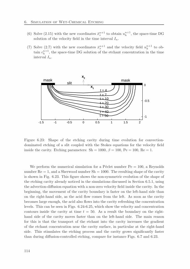
6. Simulation of Wet-Chemical Etching
(6) Solve (2.15) with the new coordinates xn+1s to obtain un+1
h , the space-time DG
solution of the velocity field in the time interval In.
(7) Solve (2.7) with the new coordinates xn+1s and the velocity field un+1
h to ob-
tain cn+1h , the space-time DG solution of the etchant concentration in the time
interval In.
-1
-0.5
0
-1.5 -1 -0.5 0 0.5 1 1.5 2
mask maskslit
x1
x2
t = 4t = 7t = 10t = 20t = 30t = 40t = 50
Figure 6.23: Shape of the etching cavity during time evolution for convection-
dominated etching of a slit coupled with the Stokes equations for the velocity field
inside the cavity. Etching parameters: Sh = 1000, β = 100, Pe = 100, Re = 1.
We perform the numerical simulation for a Peclet number Pe = 100, a Reynolds
number Re = 1, and a Sherwood number Sh = 1000. The resulting shape of the cavity
is shown in Fig. 6.23. This figure shows the non-symmetric evolution of the shape of
the etching cavity already noticed in the simulations discussed in Section 6.5.1, using
the advection-diffusion equation with a non-zero velocity field inside the cavity. In the
beginning, the movement of the cavity boundary is faster on the left-hand side than
on the right-hand side, as the acid flow comes from the left. As soon as the cavity
becomes large enough, the acid also flows into the cavity refreshing the concentration
levels. This can be seen in Figs. 6.24-6.25, which show the velocity and concentration
contours inside the cavity at time t = 50. As a result the boundary on the right-
hand side of the cavity moves faster than on the left-hand side. The main reason
for this is that the transport of the etchant into the cavity increases the gradient
of the etchant concentration near the cavity surface, in particular at the right-hand
side. This stimulates the etching process and the cavity grows significantly faster
than during diffusion-controlled etching, compare for instance Figs. 6.7 and 6.23.
114
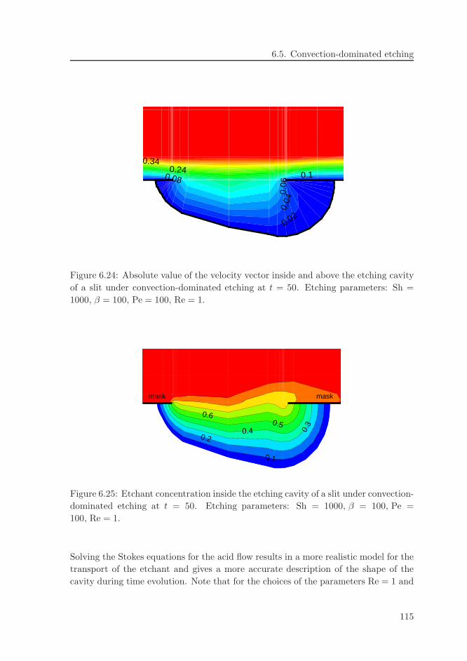
6.5. Convection-dominated etching
0.02
0.04
0.06
0.08 0.10.24
0.34
Figure 6.24: Absolute value of the velocity vector inside and above the etching cavity
of a slit under convection-dominated etching at t = 50. Etching parameters: Sh =
1000, β = 100, Pe = 100, Re = 1.
0.1
0.2
0.3
0.40.5
0.6
mask mask
Figure 6.25: Etchant concentration inside the etching cavity of a slit under convection-
dominated etching at t = 50. Etching parameters: Sh = 1000, β = 100, Pe =
100, Re = 1.
Solving the Stokes equations for the acid flow results in a more realistic model for the
transport of the etchant and gives a more accurate description of the shape of the
cavity during time evolution. Note that for the choices of the parameters Re = 1 and
115
6. Simulation of Wet-Chemical Etching
Pe = 100, the divergence of the velocity field during the simulation is not so nega-
tive. Hence the condition (4.41) in Section (4.5) is fulfilled during the computation.
However, for larger Reynolds number, we can not guarantee condition (4.41) anymore
unless the post-projection is used such as the one discussed in [24].
116
Chapter 7
Conclusions and Future Research
7.1 Conclusions
In this thesis space-time Discontinuous Galerkin (DG) finite element methods for the
equations describing transport phenomena in wet-chemical etching processes have
been developed, analyzed, and tested on real applications. In particular, we pre-
sented a space-time DG method for the advection-diffusion equation for the etchant
concentration in the acid fluid and the incompressible Navier-Stokes equations de-
scribing the flow of the acid fluid. The capability of these newly developed methods
is demonstrated for different types of wet-chemical etching processes. Here we present
the main conclusions.
First, a space-time DG method for the advection-diffusion equation in a time-
dependent computational domain has been presented. Based on a study of the DG
discretizations for second-order elliptic partial differential equations, the discretization
for the diffusive term in the advection-diffusion equation follows the method proposed
by Bassi and Rebay. A detailed analysis is given to provide stability conditions and
to prove the uniqueness of the solution of the DG discretization in a time-dependent
domain. In addition, detailed error estimates are provided and supported with nu-
merical simulations which show optimal convergence.
Also, a space-time DG method for the incompressible Navier-Stokes equations
has been developed. For this method, the algorithm proposed by Bassi and Rebay
for the discretization of the viscous term is combined with the Local Discontinuous
Galerkin (LDG) method for the discretization of the incompressibility condition and
the pressure stabilization, which has been developed by Cockburn and his coworkers.
A detailed analysis is provided to prove the stability of the space-time DG method
when using a pressure stabilization operator. The accuracy of the space-time DG
method applied to the Stokes equations is studied using numerical experiments.
The space-time discretizations are well suited to deal with problems with moving
boundaries which require deforming meshes. The capabilities of the space-time DG
117
7. Conclusions and Future Research
methods for the simulation of wet-chemical etching have been demonstrated using
different models. For this purpose special techniques were developed to generate the
initial mesh for the space-time computations. The numerical simulations of diffusion-
controlled etching of a slit and a circular hole show good agreement with the predic-
tions obtained with analytical techniques. Moreover, the numerical simulations can
give a complete description of the etching cavity during time evolution, something
that the analytical approach is not capable of.
The numerical simulations of convection-dominated etching of a slit coupled with
the Stokes equations give a detailed description of the transport phenomena in wet-
chemical etching, including the flow of the acid fluid inside the cavity. These fully
coupled simulations of convection-dominated etching clearly show the effect of the
transport of the etchant inside the cavity on the shape of the cavity which grows
much faster than under diffusion-controlled etching, but also looses symmetry.
7.2 Recommendations for future research
Here we present several recommendations for future research.
The first recommendation is related to hp-adaptation. From experience with the
simulations of wet-chemical etching, we observe that an adaptation strategy is im-
portant in order to further improve the robustness and accuracy of the numerical
simulations for wet-chemical etching processes. Making use of hp-adaptation, we can
reduce the number of elements and the degrees of freedom of the linear system re-
sulting from the discretization while maintaining the same level of accuracy. This
will reduce the computing time needed for the simulations. An additional adapta-
tion strategy should also be included in the moving boundary equation to remesh the
cavity surface resulting from the simulations.
Further study is also needed in the development of the space-time DG discretiza-
tion for the incompressible Navier-Stokes equations, in particular regarding the pres-
sure stabilization operator and the linear solvers for the resulting linear system.
Regarding the problems in wet-chemical etching, it is worth to investigate the
shape of the cavity near sharp corners, where the underetching behaves differently
than at other parts of the mask edge. Further study should also be pursued in
the direction of anisotropic wet-chemical etching and on modeling multiple chemical
reactions at the cavity surface as this phenomena also occurs in experiments. A further
validation of the simulation model with the experiments presently being conducted
will also require significant attention. Finally, improving mask designs using inverse
methods and the analysis techniques developed in this project will reduce the time
necessary to control the etching process and improve the accuracy of the objects to
be produced.
118
Appendix A
Algebraic System for the Space-Time DG
Discretizations
A.1 Algebraic system for the advection-diffusion equation
In this section we present the algebraic equations for the space-time DG discretization
of the advection-diffusion equation in the space-time slab En, which was discussed in
Section 4.4.2. We introduce the polynomial approximations ch ∈ W(pt,ps)h in each
space-time element Kj as follows:
ch(x) =
Nj∑
n=0
Cn,Kjψn,Kj
(x), (A.1)
with ψn,Kj∈ Qpt,K,ps,K
(K), where Qpt,K,ps,K(K) is defined in Section 4.3.2, and Nj =
(pt,Kj+1)(ps,Kj
+1)d. Similar expressions are used for the test functions w ∈ W(pt,ps)h .
A.1.1 Algebraic system for the diffusive part
We recall the formulation of the bilinear form for the diffusive part, given in (4.32):
ad(ch, w) =∑
K∈T nh
∫
KD∇hch · ∇hw dK
−∑
S∈SnID
∫
S
(D〈〈ch〉〉 · ∇hw +D∇hch · 〈〈w〉〉
)dS
−∑
S∈SnID
ηK
∫
S
DrS([[ch]]) · 〈〈w〉〉 dS +∑
S∈SnM
∫
S
αchw dS, (A.2)
119
A. Algebraic System for Space-Time DG Discretizations
and the diffusive part of the linear form (4.37):
ℓd(w) =−∑
S∈SnD
∫
S
gDDn · ∇hw dS
−∑
S∈SnD
ηK
∫
S
DrS(PgDn) · nw dS +∑
S∈SnM
∫
S
gMw dS. (A.3)
Note that the terms involving the lifting operator rS are written as face integrals for
simpler implementation.
First, we describe an approximation to the local lifting operator rS([[ch]]). This
approximation is derived in [59]. We consider the local lifting operator rS on S ∈∪nSn
I . If we replace the functions κ in (4.5) with 〈〈ch〉〉 and use the fact that the local
lifting operator rS has nonzero values only in the elements Ki and Kj that share the
face S, we obtain the following relation for the spatial part of the local lifting operator
rS :∫
Ki
rS,i(〈〈ch〉〉) · ϕi dK +
∫
Kj
rS,j(〈〈ch〉〉) · ϕj dK
= −1
2
∫
S
(ch,ini + ch,j nj) · (ϕi + ϕj) dS, ∀ϕi, ϕj ∈ Υ(pt,ps)h . (A.4)
Since (A.4) holds for any ϕi, ϕj ∈ Υ(pt,ps)h , we have in element Ki:
∫
Ki
rS,i(〈〈ch〉〉) · ϕi dK = −1
2
∫
S
ch,ini · ϕi dS − 1
2
∫
S
ch,j nj · ϕi dS. (A.5)
A similar expression is obtained for the lifting operator rS,j in element Kj .
We approximate the local lifting operator rS and the test functions ϕ in element
Ki as:
rS,i =
Ni∑
m=0
Rm,Kiψm,Ki
(x), ϕi =
Ni∑
l=0
Pl,Kiψl,Ki
(x). (A.6)
We then introduce the following matrices: Ai ∈ RNi×Ni , Lkij ∈ RNi×Nj , defined as:
(Anm)i =
∫
Ki
ψn,Kiψm,Ki
dK, (Lnm)kij =
∫
S
ψn,Kiψm,Kj
nkKj
dS,
where i, j refer to the element indices, and nk, with k = 1, . . . , d is the k-th component
of the space-time normal vector n on face S. We also introduce the coefficients:
Rki ∈ RNi , Ci ∈ RNi , defined as:
Rki = (Rk
0,Ki. . . Rk
Ni,Ki), Ci = (C0,Ki
. . . CNi,Ki),
with Rki the vector with the expansion coefficients of rS,i and Ci the vector with the
expansion coefficients of ch. Introducing (A.1) and (A.6) into (A.5) and using the
120
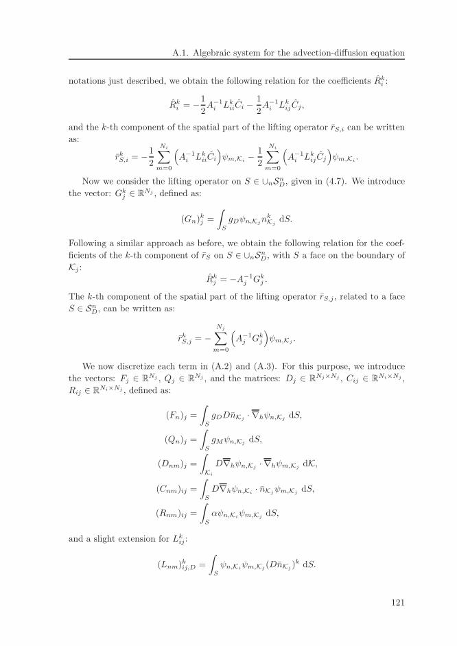
A.1. Algebraic system for the advection-diffusion equation
notations just described, we obtain the following relation for the coefficients Rki :
Rki = −1
2A−1
i LkiiCi −
1
2A−1
i LkijCj ,
and the k-th component of the spatial part of the lifting operator rS,i can be written
as:
rkS,i = −1
2
Ni∑
m=0
(
A−1i Lk
iiCi
)
ψm,Ki− 1
2
Ni∑
m=0
(
A−1i Lk
ijCj
)
ψm,Ki.
Now we consider the lifting operator on S ∈ ∪nSnD, given in (4.7). We introduce
the vector: Gkj ∈ RNj , defined as:
(Gn)kj =
∫
S
gDψn,KjnkKj
dS.
Following a similar approach as before, we obtain the following relation for the coef-
ficients of the k-th component of rS on S ∈ ∪nSnD, with S a face on the boundary of
Kj :
Rkj = −A−1
j Gkj .
The k-th component of the spatial part of the lifting operator rS,j , related to a face
S ∈ SnD, can be written as:
rkS,j = −
Nj∑
m=0
(
A−1j Gk
j
)
ψm,Kj.
We now discretize each term in (A.2) and (A.3). For this purpose, we introduce
the vectors: Fj ∈ RNj , Qj ∈ RNj , and the matrices: Dj ∈ RNj×Nj , Cij ∈ RNi×Nj ,
Rij ∈ RNi×Nj , defined as:
(Fn)j =
∫
S
gDDnKj· ∇hψn,Kj
dS,
(Qn)j =
∫
S
gMψn,KjdS,
(Dnm)j =
∫
Ki
D∇hψn,Kj· ∇hψm,Kj
dK,
(Cnm)ij =
∫
S
D∇hψn,Ki· nKj
ψm,KjdS,
(Rnm)ij =
∫
S
αψn,Kiψm,Kj
dS,
and a slight extension for Lkij :
(Lnm)kij,D =
∫
S
ψn,Kiψm,Kj
(DnKj)k dS.
121
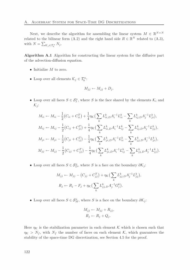
A. Algebraic System for Space-Time DG Discretizations
Next, we describe the algorithm for assembling the linear system M ∈ RN×N
related to the bilinear form (A.2) and the right hand side R ∈ RN related to (A.3),
with N =∑
Kj∈T nhNj .
Algorithm A.1 Algorithm for constructing the linear system for the diffusive part
of the advection-diffusion equation.
• Initialize M to zero.
• Loop over all elements Kj ∈ T nh :
Mjj ←Mjj +Dj.
• Loop over all faces S ∈ SnI , where S is the face shared by the elements Ki and
Kj :
Mii ←Mii −1
2
(Cii + CT
ii
)+
1
4ηK
(∑
k
Lkii,DA
−1i Lk
ii −∑
k
Lkij,DA
−1j Lk
ji
),
Mij ←Mij −1
2
(Cij + CT
ji
)+
1
4ηK
( ∑
k
Lkii,DA
−1i Lk
ij −∑
k
Lkij,DA
−1j Lk
jj
),
Mji ←Mji −1
2
(Cji + CT
ij
)− 1
4ηK
( ∑
k
Lkji,DA
−1i Lk
ii −∑
k
Lkjj,DA
−1j Lk
ji
),
Mjj ←Mjj −1
2
(Cjj + CT
jj
)− 1
4ηK
( ∑
k
Lkji,DA
−1i Lk
ij −∑
k
Lkjj,DA
−1j Lk
jj
).
• Loop over all faces S ∈ SnD, where S is a face on the boundary ∂Kj :
Mjj ←Mjj −(Cjj + CT
jj
)+ ηK
( ∑
k
Lkjj,DA
−1j Lk
jj
),
Rj ← Rj − Fj + ηK( ∑
k
Lkjj,DA
−1j Gk
j
).
• Loop over all faces S ∈ SnM , where S is a face on the boundary ∂Kj :
Mjj ←Mjj +Rjj ,
Rj ← Rj +Qj.
Here ηK is the stabilization parameter in each element K which is chosen such that
ηK > Nf , with Nf the number of faces on each element K, which guarantees the
stability of the space-time DG discretization, see Section 4.5 for the proof.
122
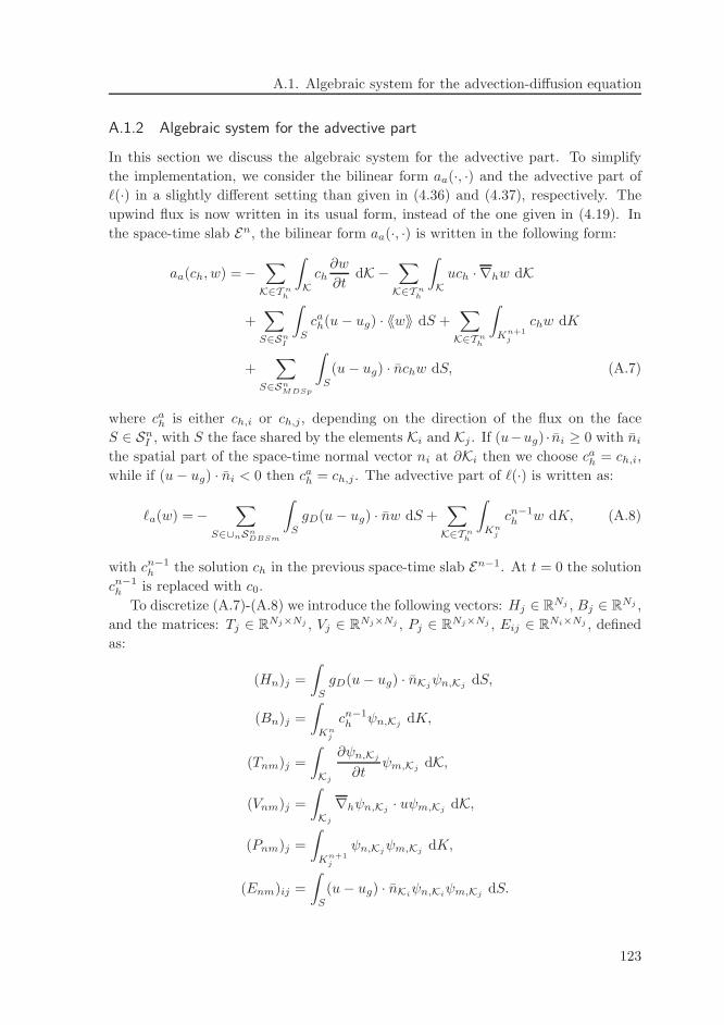
A.1. Algebraic system for the advection-diffusion equation
A.1.2 Algebraic system for the advective part
In this section we discuss the algebraic system for the advective part. To simplify
the implementation, we consider the bilinear form aa(·, ·) and the advective part of
ℓ(·) in a slightly different setting than given in (4.36) and (4.37), respectively. The
upwind flux is now written in its usual form, instead of the one given in (4.19). In
the space-time slab En, the bilinear form aa(·, ·) is written in the following form:
aa(ch, w) =−∑
K∈T nh
∫
Kch∂w
∂tdK −
∑
K∈T nh
∫
Kuch · ∇hw dK
+∑
S∈SnI
∫
S
cah(u − ug) · 〈〈w〉〉 dS +∑
K∈T nh
∫
Kn+1j
chw dK
+∑
S∈SnMDSp
∫
S
(u− ug) · nchw dS, (A.7)
where cah is either ch,i or ch,j, depending on the direction of the flux on the face
S ∈ SnI , with S the face shared by the elements Ki and Kj . If (u−ug) · ni ≥ 0 with ni
the spatial part of the space-time normal vector ni at ∂Ki then we choose cah = ch,i,
while if (u− ug) · ni < 0 then cah = ch,j . The advective part of ℓ(·) is written as:
ℓa(w) =−∑
S∈∪nSnDBSm
∫
S
gD(u − ug) · nw dS +∑
K∈T nh
∫
Knj
cn−1h w dK, (A.8)
with cn−1h the solution ch in the previous space-time slab En−1. At t = 0 the solution
cn−1h is replaced with c0.
To discretize (A.7)-(A.8) we introduce the following vectors: Hj ∈ RNj , Bj ∈ RNj ,
and the matrices: Tj ∈ RNj×Nj , Vj ∈ RNj×Nj , Pj ∈ RNj×Nj , Eij ∈ RNi×Nj , defined
as:
(Hn)j =
∫
S
gD(u− ug) · nKjψn,Kj
dS,
(Bn)j =
∫
Knj
cn−1h ψn,Kj
dK,
(Tnm)j =
∫
Kj
∂ψn,Kj
∂tψm,Kj
dK,
(Vnm)j =
∫
Kj
∇hψn,Kj· uψm,Kj
dK,
(Pnm)j =
∫
Kn+1j
ψn,Kjψm,Kj
dK,
(Enm)ij =
∫
S
(u − ug) · nKiψn,Ki
ψm,KjdS.
123
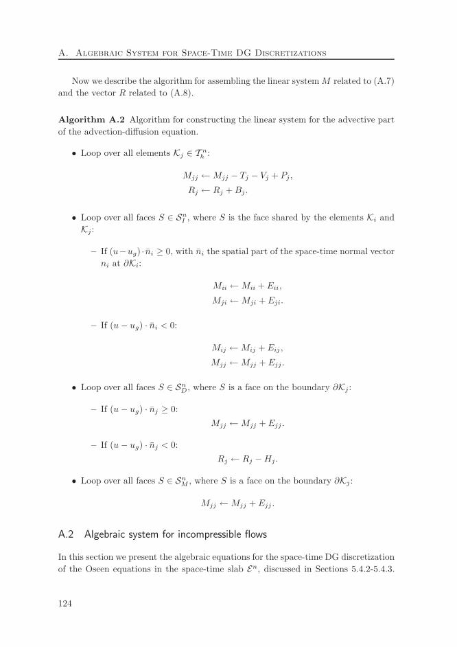
A. Algebraic System for Space-Time DG Discretizations
Now we describe the algorithm for assembling the linear systemM related to (A.7)
and the vector R related to (A.8).
Algorithm A.2 Algorithm for constructing the linear system for the advective part
of the advection-diffusion equation.
• Loop over all elements Kj ∈ T nh :
Mjj ←Mjj − Tj − Vj + Pj ,
Rj ← Rj +Bj .
• Loop over all faces S ∈ SnI , where S is the face shared by the elements Ki and
Kj :
– If (u−ug) · ni ≥ 0, with ni the spatial part of the space-time normal vector
ni at ∂Ki:
Mii ←Mii + Eii,
Mji ←Mji + Eji.
– If (u − ug) · ni < 0:
Mij ←Mij + Eij ,
Mjj ←Mjj + Ejj .
• Loop over all faces S ∈ SnD, where S is a face on the boundary ∂Kj :
– If (u − ug) · nj ≥ 0:
Mjj ←Mjj + Ejj .
– If (u − ug) · nj < 0:
Rj ← Rj −Hj .
• Loop over all faces S ∈ SnM , where S is a face on the boundary ∂Kj :
Mjj ←Mjj + Ejj .
A.2 Algebraic system for incompressible flows
In this section we present the algebraic equations for the space-time DG discretization
of the Oseen equations in the space-time slab En, discussed in Sections 5.4.2-5.4.3.
124
A.2. Algebraic system for incompressible flows
The approximations uh ∈ V (pt,ps)h , ph ∈ Q(pt,ps)
h in each space-time element Kj are
defined as follows:
uh(x) =
Nuj∑
n=0
Un,Kjψn,Kj
(x),
ph(x) =
Npj∑
n=0
Pn,Kjψn,Kj
(x), (A.9)
with ψn,Kj∈ Qpt,K,ps,K
(K), where Qpt,K,ps,K(K) is defined in Section 4.3.2, and
Nuj , N
pj the number of polynomial coefficients for uh and ph, respectively. Similar
expressions are used for the test functions v ∈ V (pt,ps)h and q ∈ Q(pt,ps)
h .
A.2.1 Algebraic system for the diffusive and convective parts
First, we recall the bilinear form Ah(·, ·), given in (5.41), but written in the following
form:
Ah(uh, v) =∑
K∈T nh
∫
Kν∇huh : ∇hv dK
−∑
S∈∪nSnID
∫
S
(ν〈〈〈uh〉〉〉 : ∇hv+ ν∇huh : 〈〈〈v〉〉〉
)dS
+∑
S∈∪nSnID
ηuK
∫
S
νLS(〈〈〈uh〉〉〉) : 〈〈〈v〉〉〉 dS, (A.10)
and the corresponding linear form Fh(·), given in (5.44):
Fh(v) =−∑
S∈∪nSnD
∫
S
νgD ⊗ n : ∇hv dS
+∑
S∈∪nSnD
ηuK
∫
S
νLS(PgD ⊗ n) : v ⊗ n dS +∑
S∈∪nSnN
∫
S
νgN · v dS. (A.11)
These forms are the space-time DG discretization for the diffusive terms in the Oseen
equations. Comparing the form Ah with the form ad in Section A.1.1, we notice
that the form Ah is an extension of the form ad to the vector functions. Hence, all
terms discussed for the algebraic equations generated by ad can be used for the l-th
component of uh by replacing the diagonal terms in the diffusion coefficient matrix
D with the viscosity coefficient ν and setting the other contributions equal to zero,
and replacing the function gM on the face S ∈ SnN with gN . The same applies for the
form ℓd in Section A.1.1 and Fh.
For the definition of the linear system for the l-th component of uh, given by
(A.10)-(A.11), we introduce the matrix M l ∈ RNu×Nu
and the vector Rl ∈ RNu
,
125
A. Algebraic System for Space-Time DG Discretizations
where Nu =∑
Kj∈T nhNu
j . The algorithm for assembling the linear system M l and
the vector Rl then follows Algorithm A.1.
Next, we recall the trilinear form Oh(·, ·; ·) given in (5.40), but reformulated in
ALE form, as follows:
Oh(uh, v;w) = −∑
K∈T nh
∫
Kuh ·
∂v
∂tdK −
∑
K∈T nh
∫
Kuh ⊗ w : ∇hv dK
+∑
K∈T nh
∫
Kn+1j
uhv dK +∑
S∈SnI
∫
S
uah ⊗ (w − ug) : 〈〈〈v〉〉〉 dS
+∑
S∈SnDp
∫
S
uh ⊗ (w − ug) : v ⊗ n dS
+∑
S∈SnN
∫
S
uh ⊗ (w − ug) : v ⊗ n dS, (A.12)
with ug the mesh velocity introduced in Section 4.4.2. The solution uah is either uh,i or
uh,j, depending of the direction of the flux on a face S ∈ SnI , where S is the face shared
by the elements Ki and Kj . If (u−ug)·ni ≥ 0 with ni the spatial par of the space-time
normal vector ni at ∂Ki then we choose uah = uh,i, while if (u − ug) · ni < 0 then
uah = uh,j. The corresponding linear form Nh(·), given in (5.43), is now formulated
in ALE form as follows:
Nh(v) =−∑
S∈∪nSnDm
∫
S
gD ⊗ (w − ug) : v ⊗ n dS +∑
K∈T nh
∫
Knj
un−1h · v dS, (A.13)
where un−1h denotes the solution in the previous space-time slab En−1, and at t = 0
this solution is replaced with the initial solution u0.
Similar to the diffusive part, we also recognize that the form Oh is an extension to
vector functions of the form aa. Hence, all terms discussed for the algebraic equations
generated by aa can be used for each component of uh inOh by replacing the advective
field u in each term with the velocity field w. The same applies for the form ℓa in
Section A.1.2 and Nh. The algorithm for assembling the linear system M l for Oh and
the right hand side Rl for Nh follows directly from Algorithm A.2.
A.2.2 Algebraic system for the pressure term and incompressibility constraint
First, we recall the bilinear form Bh, given in (5.42), which is related to the space-
time DG discretization of the pressure term and the incompressibility constraint in
the Oseen equations:
Bh(ph, v) = −∑
K∈T nh
∫
Kph∇h · v dK +
∑
S∈∪nSnID
∫
S
ph〈〈v〉〉 dS. (A.14)
126
A.2. Algebraic system for incompressible flows
To discretize the l-th component of v in (A.14) we introduce the following matrices:
W lj ∈ R
Nuj ×Np
j and Z lij ∈ R
Nui ×Np
j :
(Wnm)lj =
∫
K
∂ψn,Kj
∂xlψm,Kj
dK,
(Znm)lij =
∫
S
nlKiψn,Ki
ψm,KjdS.
Next, we consider the linear forms Gh and Hh, given in (5.45) and in (5.54),
respectively:
Gh(v) =∑
K∈T nh
∫
Kf · v dK −
∑
S∈∪nSnN
∫
S
pNv · n dS, (A.15)
Hh(q) = −∑
S∈∪nSnD
∫
S
gD · nq dS. (A.16)
To discretize each component of v in (A.15)-(A.16), we introduce the following vectors:
F lj,f ∈ R
Nuj , P l
j ∈ RNp
j , and Tj ∈ RNp
j :
(Fn)lj,f =
∫
Kj
f lψn,KjdK,
(Pn)lj =
∫
S
pNψn,KjnlKj
dS,
(Tn)j =
∫
S
gD · nKjψn,Kj
dS,
with f l the l-th component of the force vector f .
For the l-th component of v in (A.14)-(A.15), we introduce a matrix M lB ∈
RNu×Np
and vectors RlB ∈ R
Nu
, RC ∈ RNp
, where Np =∑
Kj∈T nhNp
j . The al-
gorithm for assembling the linear system M lB related to (A.14) and the right hand
sides RlB and RC related to (A.15) and (A.16), respectively, can now be summarized
as follows.
Algorithm A.3 Algorithm for constructing the linear system for the pressure con-
tribution in the Oseen equations.
• Initialize M lB to zero.
• Loop over all elements Kj ∈ T nh :
M ljj,B ←M l
jj,B −W lj ,
Rlj,B ← Rl
j,B + F lj,f .
127
A. Algebraic System for Space-Time DG Discretizations
• Loop over all faces S ∈ SnI , where S is the face shared by the elements Ki and
Kj :
M lii,B ←M l
ii,B + Z lii,
M lij,B ←M l
ij,B + Z lij ,
M lji,B ←M l
ji,B + Z lji,
M ljj,B ←M l
jj,B + Z ljj .
• Loop over all faces S ∈ SnD, where S is a face on the boundary ∂Kj :
M ljj,B ←M l
jj,B + Z ljj ,
Rj,C ← Rj,C + Tj.
• Loop over all faces S ∈ SnN , where S is a face on the boundary ∂Kj :
Rlj,B ← Rl
j,B + P lj .
A.2.3 Algebraic system for the stability term
Two types of stabilization terms are considered in Section (A.2.3). First, we consider
the stabilization term with the jump, given in (5.52):
C(1)h (ph, q) =
∑
S∈∪nSnI
∫
S
γ〈〈ph〉〉 · 〈〈q〉〉 dS. (A.17)
In order to discretize this term, we introduce the following matrix: Yij ∈ RNp
i×Np
j ,
with:
(Ynm)ij =
∫
S
γnKi· nKj
ψn,Kiψn,Kj
dS. (A.18)
We then construct a matrix M(1)C ∈ RNp×Np
related to the stabilization operator in
(A.17) as follows.
Algorithm A.4 Algorithm for constructing the linear system for the stabilization
term C(1)h .
• Initialize M(1)C to zero.
• Loop over all faces S ∈ SnI , where S is shared by the elements Ki and Kj :
M(1)ii,C ←M
(1)ii,C + Yii,
M(1)ij,C ←M
(1)ij,C + Yij ,
M(1)ji,C ←M
(1)ji,C + Yji,
M(1)jj,C ←M
(1)jj,C + Yjj .
128
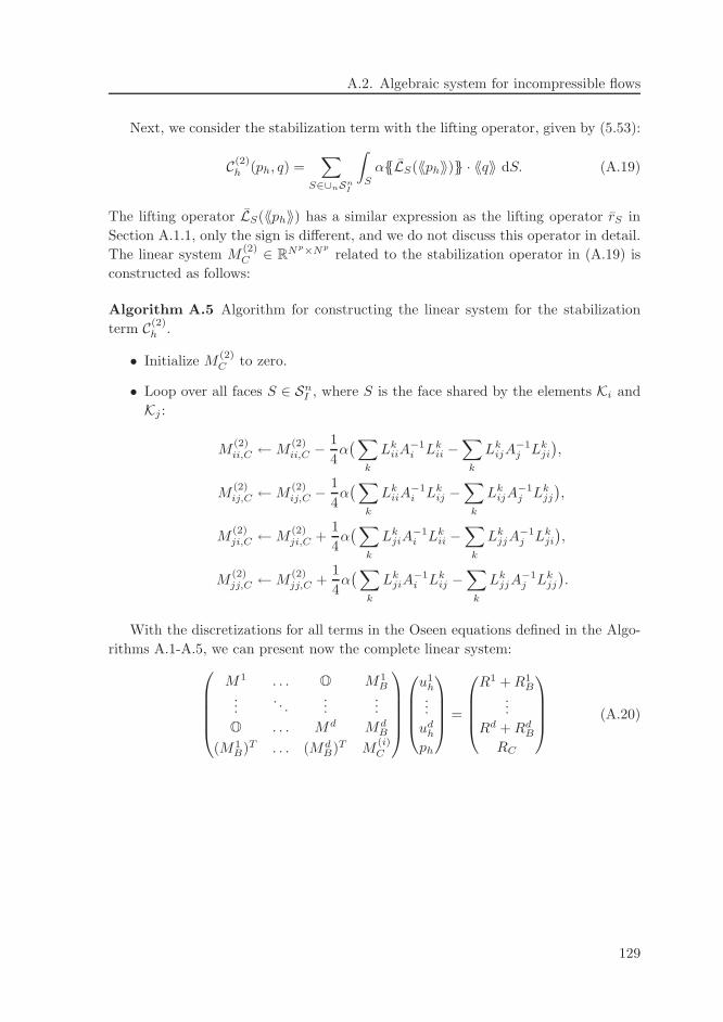
A.2. Algebraic system for incompressible flows
Next, we consider the stabilization term with the lifting operator, given by (5.53):
C(2)h (ph, q) =
∑
S∈∪nSnI
∫
S
αLS(〈〈ph〉〉) · 〈〈q〉〉 dS. (A.19)
The lifting operator LS(〈〈ph〉〉) has a similar expression as the lifting operator rS in
Section A.1.1, only the sign is different, and we do not discuss this operator in detail.
The linear system M(2)C ∈ RNp×Np
related to the stabilization operator in (A.19) is
constructed as follows:
Algorithm A.5 Algorithm for constructing the linear system for the stabilization
term C(2)h .
• Initialize M(2)C to zero.
• Loop over all faces S ∈ SnI , where S is the face shared by the elements Ki and
Kj :
M(2)ii,C ←M
(2)ii,C −
1
4α( ∑
k
LkiiA
−1i Lk
ii −∑
k
LkijA
−1j Lk
ji
),
M(2)ij,C ←M
(2)ij,C −
1
4α( ∑
k
LkiiA
−1i Lk
ij −∑
k
LkijA
−1j Lk
jj
),
M(2)ji,C ←M
(2)ji,C +
1
4α( ∑
k
LkjiA
−1i Lk
ii −∑
k
LkjjA
−1j Lk
ji
),
M(2)jj,C ←M
(2)jj,C +
1
4α( ∑
k
LkjiA
−1i Lk
ij −∑
k
LkjjA
−1j Lk
jj
).
With the discretizations for all terms in the Oseen equations defined in the Algo-
rithms A.1-A.5, we can present now the complete linear system:
M1 . . . O M1B
.... . .
......
O . . . Md MdB
(M1B)T . . . (Md
B)T M(i)C
u1h...
udh
ph
=
R1 +R1B
...
Rd +RdB
RC
(A.20)
129

Appendix B
Anisotropic Interpolation Error Estimates
B.1 Preliminaries
In this appendix, we derive in more detail the anisotropic interpolation error estimates
discussed in Section 4.6.1. The derivations follow the analysis in [31], but are extended
to general dimensions, such that they can be applied in the analysis of the space-time
discretization.
First, we recall the construction of the space-time elements K introduced in Sec-
tion 4.3.2. Each space-time element K is the image of a fixed master element K,
with K an open unit hypercube in Rd+1. We define in K reference coordinates
x = (x0, x1, . . . , xd). The space-time element K is constructed via two mappings
FK and QK, where FK : K → K is an affine mapping and QK : K → K is a (regular
enough) diffeomorphism (see Fig. 4.2). The element K is defined with respect to the
coordinates x = (x0, x1, . . . , xd). We denote by hi, i = 1, . . . , d the edge length of
K in the xi direction, and nt the edge length in the x0 direction. The boundaries
∂Ki, ∂Ki, ∂Ki denote the boundary face with respectively the xi, xi, and xi coordinate
constant.
We also recall the definition of anisotropic Sobolev spaces given in Section 4.3.2.
Note that the definition of anisotropy is restricted to the case where the Sobolev
index can be different for the temporal and spatial variables. All spatial variables
have, however, the same index.
Definition B.1 Let (st, ss) be a pair of non-negative integers, where st, ss correspond
to the temporal and spatial Sobolev index, respectively. The anisotropic Sobolev space
of order (st, ss) on an element K is defined as
H(st,ss)(K) := w ∈ L2(K) : ∂γt∂γsw ∈ L2(K) for 0 ≤ γt ≤ st, 0 ≤ |γs| ≤ ss,
131
B. Anisotropic Interpolation Error Estimates
while on an element K, the anisotropic Sobolev space is defined as
H(st,ss)(K) := w ∈ L2(K) : w QK ∈ H(st,ss)(K).
Next, we introduce the spaces of polynomials associated with the finite element
spaces given in Section 4.3.2.
Definition B.2 Let I ≡ (−1, 1) and K ≡ (−1, 1)d+1. On the interval I we define the
space of polynomials Pp(I) by
Pp(I) := spanxi : i = 0, . . . , p.
Furthermore, we define the anisotropic tensor-product polynomial space Qpt,K,ps,K(K)
by
Qpt,K,ps,K(K) :=Ppt,K
(I)⊗ Pps,K(I)⊗ . . .⊗ Pps,K
(I)︸ ︷︷ ︸
d×
=spanxi0x
m11 . . . xmd
d : i = 0, . . . , pt,K;m1, . . . ,md = 0, . . . , ps,K,
where pt,K, ps,K are local polynomial degrees, in time and space, respectively.
We introduce a one-dimensional L2 projection operator in the following definition.
Definition B.3 Let u ∈ L2(I) and let Pp(I) be the space of polynomials on I of
degree p or less. We define the L2 projection operator
πp : L2(I)→ Pp(I),
by
πpu(x) :=
p∑
n=0
anLn(x),
where
an =2n+ 1
2
∫
I
u(x)Ln(x) dx,
with Ln the Legendre polynomial of degree n defined on I. It is easy to show that
the linear operator πp is idempotent with norm ‖πp‖L2(I)→Pp(I) = 1.
The following lemma, which is taken from [31] (Lemmas 3.2, 3.3, and 3.5), states
several one-dimensional estimates.
Lemma B.4 Let u ∈ Hk+1(I), with integer k ≥ 0. Let πpu be the L2-projection of u
onto Pp(I), p ≥ 0. Then for every integer s, with 0 ≤ s ≤ min(p+ 1, k + 1), we have
the estimates:
‖u− πpu‖0,I ≤ Φ1(p+ 1, s)‖u(s)‖0,I , (B.1)
132
B.1. Preliminaries
with u(s) = dsudxs , and for every integer t, with 0 ≤ t ≤ min(p, k):
‖πpu′ − (πpu)
′‖0,I ≤ CL2
p Φ1(p, t)‖u(t+1)‖0,I , (B.2)
where the parameter CL2
p depends on p, with CL2
0 = 0, CL2
1 = 36/15, and CL2
p =√2p+ 2, and a prime denotes differentiation. Moreover, we have
‖u′ − (πpu)′‖0,I ≤ (1 + CL2
p )Φ1(p, t)‖u(t+1)‖0,I , (B.3)
with Φ1(p, s) :=(Γ(p−s+1)
Γ(p+s+1)
) 12 , and Γ the gamma function, see for instance [1]. At the
boundary of I, we have the following estimate:
|u− πpu(±1)| ≤ Φ1(p, t)√2p+ 1
‖u(t+1)‖0,I . (B.4)
We also introduce the projection operator P : L2(K)→ Qpt,K,ps,K(K).
Definition B.5 Let K ≡ (−1, 1)d+1. We define the L2-projection operator
P : L2(K)→ Qpt,K,ps,K(K),
by
P := π0ptπ1
ps. . . πd
ps,
where π0pt, π1
ps, . . . , πd
psdenote the one-dimensional L2 projection given in Definition
B.3. The superscripts 0, 1, . . . , d refer to the coordinate direction in which the one-
dimensional projection is applied.
In the following lemma, we present a trace inequality for an anisotropic element.
This lemma is a direct extension from [31], Lemma A.1, to a space-time discretization
in d+ 1 dimensions.
Lemma B.6 Let u ∈ H(kt,ks)(K) with kt, ks ≥ 1, K an axiparallel element, with
nt, h1, . . . , hd the length of its edges. Then the following trace inequality holds:
‖u‖20,∂Ki
≤ 2
hi‖u‖2
0,K + 4‖u‖0,K‖∂iu‖0,K,
for i = 0, . . . , d, and h0 = nt.
The next lemma, which provides scaling identities between Sobolev seminorms on
the reference element K and on the axiparallel element K, will be needed for deriving
estimates on a space-time element K. This lemma is a direct extension from [31],
Lemma A.3, to a space-time discretization in d+ 1 dimensions.
133
B. Anisotropic Interpolation Error Estimates
Lemma B.7 Let u ∈ H(kt,ks)(K), and K an axiparallel element with nt, h1, . . . , hd
the length of its edges. On element K, the following scaling identity holds for 0 ≤ l ≤kt, 0 ≤ m1, . . . ,md ≤ ks:
‖∂l0∂
m11 . . . ∂md
d u‖20,K=
(nt
2
)2l−1(h1
2
)2m1−1
. . .(hd
2
)2md−1
‖∂l0∂
m11 . . . ∂md
d u‖20,K,
where u := u FK and ∂i, ∂i denote the partial derivatives in respectively the xi and
xi coordinate directions. On the part of the element boundary ∂Ki with i = 1, . . . , d,
we have:
‖∂l0∂
m11 . . . ∂md
d u‖20,∂Ki
=(nt
2
)2l−1(hi
2
)(h1
2
)2m1−1
. . .(hd
2
)2md−1
‖∂l0∂
m11 . . . ∂md
d u‖20,∂Ki
,
(B.5)
and on the boundary ∂K0 we have:
‖∂l0∂
m11 . . . ∂md
d u‖20,∂K0
=(nt
2
)2l(h1
2
)2m1−1
. . .(hd
2
)2md−1
‖∂l0∂
m11 . . . ∂md
d u‖20,∂K0
.
(B.6)
B.2 Interpolation error estimates on the reference element
In this section we discuss the interpolation error estimates on the reference element K.
The first two lemmas are extensions to a space-time discretization in d+1 dimensions
of the result given in [31], Lemma 3.7.
Lemma B.8 Let u ∈ H(kt+1,ks+1)(K) and kt, ks ≥ 0. Let Pu be the L2-projection of
u onto Qpt,K,ps,K(K). Then we have an estimate
‖u−P u‖0,K ≤ Φ1(ps,K + 1, sK)
d∑
i=1
‖∂sK
i u‖0,K + Φ1(pt,K +1, s0,K)‖∂s0,K
0 u‖0,K, (B.7)
with 0 ≤ sK ≤ min(ps,K + 1, ks + 1) and 0 ≤ s0,K ≤ min(pt,K + 1, kt + 1).
Proof . We show the proof for d = 3. The proof for other dimensions is similar.
Using the tensor product nature of the projection operator, we decompose u− P u as
u− Pu = u− π0ptu+ π0
pt
(
u− π1psu+ π1
ps
(u− π2
psu+ π2
ps(u− π3
psu)
))
,
and apply the triangle inequality to obtain
‖u− P u‖0,K ≤‖u− π0ptu‖0,K + ‖π0
pt(u− π1
psu)‖0,K
+ ‖π0ptπ1
ps(u− π2
psu)‖0,K + ‖π0
ptπ1
psπ2
ps(u − π3
psu)‖0,K.
134
B.2. Interpolation error estimates on the reference element
Since the projection operators π0pt, π1
ps, π2
ps, π3
psare bounded with norm equal to one,
we then obtain:
‖u− Pu‖0,K ≤3∑
i=1
‖u− πipsu‖0,K + ‖u− π0
ptu‖0,K.
Using Fubini’s theorem to separate the integrals in the norms on the right-hand side
into a product of one dimensional integrals and applying (B.1) to each term completes
the proof.
Lemma B.9 Let u ∈ H(kt+1,ks+1)(K) and kt, ks ≥ 0. Let P u be the L2-projection
of u onto Qpt,K,ps,K(K). Denoting the partial derivative in the xi direction as ∂i, for
i = 1, . . . , d, we have the following estimate:
‖∂i(u− P u)‖0,K ≤(1 + CL2
ps,K)Φ1(ps,K, tK)‖∂tK+1
i u‖0,K
+ Φ1(ps,K + 1, qK)d∑
j=1,j 6=i
‖∂qKj ∂iu‖0,K
+ Φ1(pt,K + 1, q0,K)‖∂q0,K
0 ∂iu‖0,K, (B.8)
with 0 ≤ qK ≤ min(ps,K + 1, ks), 0 ≤ q0,K ≤ min(pt,K + 1, kt), and 0 ≤ tK ≤min(ps,K, ks).
Proof . We show the proof for d = 3 and i = 1. The proof for the other coordinate
directions and dimensions is similar. We have:
‖∂1(u − Pu)‖0,K ≤ ‖∂1u− P(∂1u)‖0,K + ‖P(∂1u)− ∂1Pu‖0,K = T1 + T2.
Using Lemma B.8 with u replaced by ∂1u, the term T1 is bounded as follows
T1 ≤Φ1(ps,K + 1, tK)‖∂tK+11 u‖0,K + Φ1(ps,K + 1, qK)
∑
j=2,3
‖∂qKj ∂1u‖0,K
+ Φ1(pt,K + 1, q0,K)‖∂q0,K
0 ∂1u‖0,K.
Using the commutativity of ∂1 with π0pt, π2
ps, π3
psand the fact that π0
pt, π2
ps, π3
psare
idempotent, we have for the term T2:
T2 = ‖π3psπ2
psπ0
pt(π1
ps(∂1u)− ∂1π
1psu)‖0,K ≤ ‖π1
ps(∂1u)− ∂1π
1psu‖0,K.
Then, using (B.2) and Fubini’s theorem we have
T2 ≤ CL2
ps,KΦ1(ps,K, tK)‖∂tK+1
1 u‖0,K.
Adding the terms T1 and T2, and noting that Φ1(ps,K + 1, tK) ≤ Φ1(ps,K, tK), the
result follows.
Next, we present an interpolation error estimate on the boundary of the reference
element ∂K. This estimate is an extension of the result given in [31], Lemma 3.8, to
a space-time discretization in d+ 1 dimensions.
135
B. Anisotropic Interpolation Error Estimates
Lemma B.10 Let u ∈ H(kt+1,ks+1)(K) with integers kt, ks ≥ 0. Let P u be the L2-
projection of u onto Qpt,K,ps,K(K). Denoting with ∂Ki that part of ∂K where xi = ±1,
we have for i = 1, . . . , d the following estimate:
‖u− Pu‖0,∂Ki≤Φ1(ps,K, tK)
√2ps,K + 1
‖∂tK+1i u‖0,K
+√
3Φ1(ps,K + 1, sK)
d∑
j=1,j 6=i
‖∂sK
j u‖0,K
+(√
2 +1
√2ps,K + 1
)Φ1(ps,K + 1, qK)
d∑
j=1,j 6=i
‖∂qKj ∂iu‖0,K
+√
3Φ1(pt,K + 1, s0,K)‖∂s0,K
0 u‖0,K
+(√
2 +1
√2ps,K + 1
)Φ1(pt,K + 1, q0,K)‖∂q0,K
0 ∂iu‖0,K, (B.9)
while on ∂K0, which is the part of ∂K where x0 = ±1, we have the estimate:
‖u− P u‖0,∂K0≤Φ1(pt,K, t0,K)
√2pt,K + 1
‖∂t0,K+10 u‖0,K
+√
3Φ1(ps,K + 1, sK)
d∑
i=1
‖∂sK
i u‖0,K
+(√
2 +1
√2pt,K + 1
)Φ1(ps,K + 1, qK)
d∑
i=1
‖∂qKi ∂0u‖0,K, (B.10)
with 0 ≤ sK ≤ min(ps,K + 1, ks + 1), 0 ≤ s0,K ≤ min(pt,K + 1, kt + 1), 0 ≤ qK ≤min(ps,K + 1, ks), 0 ≤ s0,K, q0,K ≤ min(pt,K + 1, kt), 0 ≤ tK ≤ min(ps,K, ks), and
0 ≤ t0,K ≤ min(pt,K, kt).
Proof . We show the proof for d = 3 and i = 1. The proof for the other coordinate
directions and dimensions is similar. We decompose the projector P as:
P = π1psπm,
with πm = π0ptπ2
psπ3
ps. Using the triangle inequality, we have:
‖u− P u‖0,∂K1≤ ‖u− π1
psu‖0,∂K1
+ ‖π1ps
(u − πmu)‖0,∂K1= A1 +A2.
For the term A2, we proceed as follows. We define w = u − πmu and write
π1psw = w + (π1
psw − w). Then, using (B.4) with t = 0, we obtain
A2 ≤ ‖w‖0,∂K1+ ‖w − π1
psw‖0,∂K1
,
≤ ‖w‖0,∂K1+
1√
2ps,K + 1‖∂1w‖0,K,
= A21 +A22.
136
B.3. Interpolation error estimates on the space-time element
Using the trace inequality, given in Lemma B.6, and the arithmetic-geometric mean
inequality, we then obtain for the term A21:
A21 ≤(‖w‖2
0,K + 4‖w‖0,K‖∂1w‖0,K) 1
2 ,
≤(‖w‖2
0,K + 2‖w‖20,K + 2‖∂1w‖20,K
) 12 ,
and using the fact that√a+ b ≤ √a+
√b, we have:
A21 ≤√
3‖w‖0,K +√
2‖∂1w‖0,K.
Adding up all terms together, we then obtain:
‖u− P u‖0,∂K1≤‖u− π1
psu‖0,∂K1
+√
3‖u− πmu‖0,K
+(√
2 +1
√2ps,K + 1
)‖∂1(u− πmu)‖0,K.
We use (B.4) for the first term and Lemma B.8 with respect to πm for the second
term. For the third term, we first observe that ∂1(u− πmu) = ∂1u− πm∂1u. Further
application of Lemma B.8 with u replaced by ∂1u and P with πm completes the proof.
The proof for the estimate on the boundary ∂K0 is analogous.
B.3 Interpolation error estimates on the space-time element
In this section we derive interpolation error estimates on a space-time element K.
First, we define the projection operators on K and K, respectively, using the mappings
FK and QK, see also [31], Section 3.1.3.
Definition B.11 Let u : K → R and u : K → R and assume there exist one-to-one
and invertible mappings FK : K → K, QK : K → K. We define the L2-projection
operator P on K by the relation
Pu := (P(u FK)) F−1K , ∀u ∈ L2(K),
where, as before, P denotes the L2-projector on the reference element K. Moreover,
we define the L2-projection operator P on K by
Pu := (P(u QK)) Q−1K , ∀u ∈ L2(K).
We denote by JQKthe Jacobian matrix of the mapping QK and introduce the
following notations:
CQK:= ‖ detJQK
‖12
0,∞,K,
C′
QK:= ‖(detJQK
)−1‖12
0,∞,K,
CmnQK
:= ‖ detJQK\mn‖0,∞,K,
C∂i
QK:= ‖ det(J∂Ki
)‖12
0,∞,K,
137
B. Anisotropic Interpolation Error Estimates
with JQK\mn the submatrix of JQKobtained by deleting the m-th row and n-th
column and J∂Kithe surface measure of the boundary ∂Ki.
First, we extend the interpolation estimates in Lemma B.8 to functions defined
on K.
Lemma B.12 Assume that K is a space-time element in Rd+1 constructed via two
one-to-one and invertible mappings QK, FK, with FK : K → K and QK : K → K.
Assume also that hi, i = 1, . . . , d is the edge length of K in the xi direction, and nt
the edge length in the x0 direction. Let u ∈ H(kt+1,ks+1)(K), with kt, ks ≥ 0, and Pbe the L2 projection of u on K. Then we have the following estimate:
‖u− Pu‖0,K ≤CQKΦ1(ps,K + 1, sK)
d∑
i=1
(hi
2
)sK
‖∂sK
i u‖0,K
+ CQKΦ1(pt,K + 1, s0,K)
(nt
2
)s0,K
‖∂s0,K
0 u‖0,K, (B.11)
with 0 ≤ sK ≤ min(ps,K + 1, ks + 1) and 0 ≤ s0,K ≤ min(pt,K + 1, kt + 1).
Proof . First, using the definition of the projection operators P and P , we have
the following bound:
‖u− Pu‖0,K ≤ CQK‖u− Pu‖0,K ≤ CQK
CFK‖u− Pu‖0,K,
with
CFK=
(nt
2
) 12(h1
2
) 12
. . .(hd
2
) 12
.
Using Lemma B.8 and the scaling identities given in Lemma B.7, we have:
‖u− Pu‖0,K ≤ CQKΦ1(ps,K + 1, sK)
d∑
i=1
(hi
2
)sK
‖∂sK
i u‖0,K
+ CQKΦ1(pt,K + 1, s0,K)
(nt
2
)s0,K
‖∂s0,K
0 u‖0,K,
for 0 ≤ sK ≤ min(ps,K+1, ks+1) and 0 ≤ s0,K ≤ min(pt,K+1, kt+1). This completes
the proof.
Next, we extend the interpolation estimates in Lemma B.9 to functions defined
on K.
Lemma B.13 Assume that K is a space-time element in Rd+1 constructed via two
one-to-one and invertible mappings QK, FK, with FK : K → K and QK : K → K.
Assume also that hi, i = 1, . . . , d is the edge length of K in the xi direction, and nt
the edge length in the x0 direction. Let u ∈ H(kt+1,ks+1)(K), with kt, ks ≥ 0, and Pbe the L2 projection of u on K. Then we have the following estimate:
‖∂i(u− Pu)‖0,K ≤ αiiMi +∑
j 6=i
αijMj, (B.12)
138
B.3. Interpolation error estimates on the space-time element
where:
Mi =(1 + CL2
ps,K)Φ1(ps,K, tK)
(hi
2
)tK‖∂tK+1
i u‖0,K
+ Φ1(ps,K + 1, tK + 1)
d∑
j=1,j 6=i
(hj
2
)tK+1
‖∂tK+1j ∂iu‖0,K
+(nt
2
)t0,K+1
Φ1(pt,K + 1, t0,K + 1)‖∂t0,K+10 ∂iu‖0,K,
for i = 1, . . . , d, with αii =√
2CiiQKC
′
QK, αmn =
√2Cmn
QKC
′
QK,m 6= n, and 0 ≤ tK ≤
min(ps,K, ks), 0 ≤ t0,K ≤ min(pt,K, kt), .
Proof . Using the chain rule and the arithmetic-geometric mean inequality, we
obtain:
‖∂i(u− Pu)‖20,K ≤2
∫
K
(
∂i((u− Pu) QK) Q−1K∂xi
∂xi
)2
dK
+ 4
d∑
j=1,j 6=i
∫
K
(
∂j((u − Pu) QK) Q−1K∂xj
∂xi
)2
dK.
Using the mapping Q−1K from K to K we then obtain:
‖∂i(u−Pu)‖0,K ≤√
2C′
QKCii
QK‖∂i(u− Pu)‖0,K + 2C
′
QK
d∑
j=1,j 6=i
CijQK‖∂j(u− Pu)‖0,K.
Now we want to estimate the term ‖∂i(u − P u)‖K, for i = 1, . . . , d. Using the
change of variables from u to u, Lemma B.9 and the scaling identities given in Lemma
B.7, we obtain:
‖∂i(u− P u)‖0,K ≤(1 + CL2
ps,K)Φ1(ps,K, tK)
(hi
2
)tK‖∂tK+1
i u‖0,K
+ Φ1(ps,K + 1, tK + 1)
d∑
j=1,j 6=i
(hj
2
)tK+1
‖∂tK+1j ∂iu‖0,K
+(nt
2
)t0,K+1
Φ1(pt,K + 1, t0,K + 1)‖∂t0,K+10 ∂iu‖0,K.
This completes the proof.
Finally, we derive an estimate on the boundary of element ∂K.
Lemma B.14 Assume that K is a space-time element in Rd+1 constructed via two
one-to-one and invertible mappings QK, FK, with FK : K → K and QK : K → K.
Assume also that hi, i = 1, . . . , d is the edge length of K in the xi direction, and nt
the edge length in the x0 direction. Let u ∈ H(kt+1,ks+1)(K), with kt, ks ≥ 0 and
139
B. Anisotropic Interpolation Error Estimates
P be the L2 projection of u on K. On the boundaries ∂Ki, i = 1, . . . , d we have the
following estimate:
‖u− Pu‖0,∂Ki≤ C∂i
QKM∂
i , (B.13)
where
M∂i =
Φ1(ps,K, tK)√
2ps,K + 1
(hi
2
)tK+ 12 ‖∂tK+1
i u‖0,K
+√
3(hi
2
)− 12
Φ1(ps,K + 1, sK)
d∑
j=1,j 6=i
(hj
2
)sK
‖∂sK
j u‖0,K
+(hi
2
) 12 (√
2 +1
√2ps,K + 1
)Φ1(ps,K + 1, qK)
d∑
j=1,j 6=i
(hj
2
)qK‖∂qK
j ∂iu‖0,K
+√
3(hi
2
)− 12
Φ1(pt,K + 1, s0,K)(nt
2
)s0,K
‖∂s0,K
0 u‖0,K
+(hi
2
) 12 (√
2 +1
√2ps,K + 1
)Φ1(pt,K + 1, q0,K)
(nt
2
)q0,K
‖∂q0,K
0 ∂iu‖0,K,
while on the boundary ∂K0 we have the following estimate:
‖u− Pu‖0,∂K0 ≤ C∂0
QKM∂
0 , (B.14)
where
M∂0 =
Φ1(pt,K, t0,K)√
2pt,K + 1
(nt
2
)t0,K+ 12 ‖∂t0,K+1
0 u‖0,K
+√
3(nt
2
)− 12
Φ1(ps,K + 1, sK)
d∑
i=1
(hi
2
)sK
‖∂sK
i u‖0,K
+(nt
2
) 12 (√
2 +1
√2pt,K + 1
)Φ1(ps,K + 1, qK)
d∑
i=1
(hi
2
)qK‖∂qK
i ∂0u‖0,K,
with 0 ≤ sK ≤ min(ps,K + 1, ks + 1), 0 ≤ s0,K ≤ min(pt,K + 1, kt + 1), 0 ≤ qK ≤min(ps,K + 1, ks), 0 ≤ q0,K ≤ min(pt,K + 1, kt), and 0 ≤ tK ≤ min(ps,K, ks), 0 ≤t0,K ≤ min(pt,K, kt).
Proof . First, using the change of variables, we have:
‖u− Pu‖0,∂Ki≤ C∂i
QK‖u− P u‖0,∂Ki
, for i = 0, 1, . . . , d.
Then, using Lemma B.10 and the scaling identities on the boundary ∂Ki, i = 1, . . . , d,
given in Lemma B.7, we have:
‖u− P u‖0,∂Ki≤M∂
i ,
140
B.3. Interpolation error estimates on the space-time element
while on the boundary ∂K0 we obtain:
‖u− Pu‖0,∂K0≤M∂
0 .
This completes the proof.
141

Bibliography
[1] M. Abramowitz & I.A. Stegun, Handbook of Mathematical Functions, Dover Publi-
cations, New York, 1972.
[2] M. Ainsworth & B. Senior, An Adaptive Refinement Strategy for hp-Finite Element
Computations, Appl. Num. Math., 26, 165-178, 1998.
[3] D.N. Arnold, An Interior Penalty Finite Element Method with Discontinuous Ele-
ments, SIAM J. Num. Anal., 19 (4), 742-760, 1982.
[4] D.N. Arnold, F. Brezzi, B. Cockburn, & L.D. Marini, Unified Analysis of Dis-
continuous Galerkin Methods for Elliptic Problems, SIAM J. Num. Anal., 39 (5), 1749-
1779, 2002.
[5] F. Bassi, S. Rebay, G. Mariotti, S. Pedinotti, & M. Savini, A High-Order Ac-
curate Discontinuous Finite Element Method for Inviscid and Viscous Turbomachinery
Flows, in Proceedings of 2nd European Conference on Turbomachinery, Fluid Dynamics
and Thermodynamics, Technologisch Instituut, Antwerpen, Belgium, 99-108, 1997.
[6] F. Bassi & S. Rebay, A High-Order Accurate Discontinuous Finite Element Method
for the Numerical Solution of the Compressible Navier-Stokes Equations, J. Comput.
Phys., 131, 267-279, 1997.
[7] F. Bassi & S. Rebay, Numerical Evaluation of Two Discontinuous Galerkin Methods
for the Compressible Navier-Stokes Equations, Int. J. Numer. Meth. Fluids, 40, 197-
207, 2002.
[8] F. Bassi, A. Crivellini, D.A. Di Pietro, & S. Rebay, An Artificial Compressibil-
ity Flux for the Discontinuous Galerkin Solution of the Incompressible Navier-Stokes
Equations, submitted to J. Comput. Phys., 2005.
[9] C.E. Baumann & J.T. Oden, A Discontinuous hp Finite Element Method for
Convection-Diffusion Equations, Comput. Methods Appl. Engrg., 175, 311-341, 1999.
[10] C.E. Baumann & J.T. Oden, A Discontinuous hp Finite Element Method for the
Euler and Navier-Stokes Equations, Int. J. Numer. Meth. Fluids, 31, 79-95, 1999.
[11] S.C. Brenner & L.R. Scott, The Mathematical Theory of Finite Element Methods,
2nd ed., Springer-Verlag, 2002.
143
Bibliography
[12] F. Brezzi, G. Manzini, D. Marini, P. Pietra, & A. Russo, Discontinuous Galerkin
Approximations for Elliptic Problems, Numer. Methods Partial Differential Eq., 16,
365-378, 2000.
[13] F. Brezzi, L.D. Marini, & E. Suli, Discontinuous Galerkin Methods for First-Order
Hyperbolic Problems, Math. Models Methods Appl. Sci., 14 (12), 1893-1903, 2004.
[14] P. Castillo, B. Cockburn, I. Perugia, & D. Schotzau, Local Discontinuous
Galerkin Methods for Elliptic Problems, Commun. Numer. Meth. Engng, 18, 69-75,
2002.
[15] B. Cockburn & P.A. Gremaud, Error Estimates for Finite Element Methods for
Nonlinear Conservation Laws, SIAM. J. Num. Anal., 33, 522-554, 1996.
[16] B. Cockburn & C.W. Shu, The Local Discontinuous Galerkin Method for Time-
Dependent Convection-Diffusion Systems, SIAM. J. Num. Anal., 35 (6), 2440-2463,
1998.
[17] B. Cockburn, Discontinuous Galerkin Methods for Convection Dominated Problems,
in High-Order Methods for Computational Physics, T. Barth & H. Deconink (editors),
Springer-Verlag, 1999.
[18] B. Cockburn, G. Karniadakis, & C.W. Shu, Discontinuous Galerkin Methods.
Theory, Computation and Applications, Springer-Verlag, 2000.
[19] B. Cockburn & C.W. Shu, Runge Kutta Discontinuous Galerkin Method for
Convection-Dominated Problems, J. Sci. Comput., 6 (3), 173-261, 2001.
[20] B. Cockburn, G. Kanschat, I. Perugia, & D. Schotzau, Superconvergence of the
Local Discontinuous Galerkin Method for Elliptic Problems on Cartesian Grids, SIAM
J. Numer. Anal., 39 (1), 264-285, 2002.
[21] B. Cockburn, G. Kanschat, D. Schotzau, & C. Schwab, Local Discontinuous
Galerkin Methods for the Stokes Systems, SIAM J. Numer. Anal., 40 (1), 319-343,
2002.
[22] B. Cockburn, G. Kanschat, & D. Schotzau, The Local Discontinuous Galerkin
Method in Incompressible Fluid Flow, in Proceedings of Fifth World Congress on Com-
putational Mechanics V, 2002.
[23] B. Cockburn, G. Kanschat, & D. Schotzau, The Local Discontinuous Galerkin
Method for the Oseen Equations, Math. Comput., 73, 569-593, 2004.
[24] B. Cockburn, G. Kanschat, & D. Schotzau, A Locally Conservative LDG Method
for the Incompressible Navier-Stokes Equations, Math. Comput., 74, 1067-1095, 2004.
[25] R.M.J. van Damme & J.J. Sudirham, Optimal hp Adaptive Methods for Discontinu-
ous Galerkin methods, in preparation.
[26] L. Demkowicz, W. Rachowicz, & Ph. Devloo, A Fully Automatic hp-Adaptivity,
J. Sci. Comput., 17 (1-4), 117-142, 2002.
144
[27] L. Demkowicz, Projection-Based Interpolation, internal report ICES 04-03, 2004.
[28] J. Jr. Douglas & T. Dupont, Interior Penalty Procedures for Elliptic and Parabolic
Galerkin Methods, in Lecture Notes in Physics, 58, Springer-Verlag, 1976.
[29] C.H. Driesen, Simulation of Convection-Driven Wet-Chemical Etching, PhD Thesis,
University of Twente, 1999.
[30] K.J. Fidkowski & P.F. Fischer, A Discontinuous Galerkin Multigrid Method for the
Incompressible Navier-Stokes Equations, internal report, Dept. Aerospace Engineering,
Massachusetts Institute of Technology, 2004.
[31] E.H. Georgoulis, Discontinuous Galerkin Methods on Shaped-Regular and
Anisotropic Meshes, PhD Thesis, Christ Church, University of Oxford, 2003.
[32] V. Girault & P.-A. Raviart, Finite Element Methods for Navier-Stokes Equations.
Theory and Algorithms, Springer-Verlag, 1986.
[33] P. Grisvard, Elliptic Problems in Nonsmooth Domains, Pitman Advanced Pub. Pro-
gram, 1985.
[34] W. Gui & I. Babuska, The h, p, and hp Versions of the Finite Element Method in
1 Dimension, Part I. The Error Analysis of the p-Version, Numer. Math., 49, 577-612,
1986.
[35] W. Gui & I. Babuska, The h, p, and hp Versions of the Finite Element Method in 1
Dimension, Part II. The Error Analysis of the h- and hp Versions, Numer. Math., 49,
613-657, 1986.
[36] W. Gui & I. Babuska, The h, p, and hp Versions of the Finite Element Method in 1
Dimension, Part III. The Adaptive hp Version, Numer. Math., 49, 659-683, 1986.
[37] J. Haneveld, H. Jansen, E. Berenschot, N. Tas, & M. Elwenspoek, Wet-
Anisotropic Etching for Fluidic 1D Nanochannels, J. Micromech. Microeng., 13, S62-
S66, 2003.
[38] P. Houston, C. Schwab, & E. Suli, Discontinuous hp-Finite Element Methods for
Advection-Diffusion-Reaction Problems, SIAM J. Numer. Anal., 39 (6), 2133-2163,
2002.
[39] P. Houston, B. Senior, & E. Suli, Sobolev Regularity Estimation for hp-Adaptive
Finite Element Methods, in Numerical Mathematics and Advanced Applications, F.
Brezzi, A. Buffa, S. Corsaro, & A. Murli (editors), Springer-Verlag, 619-644, 2003.
[40] P. Houston, D. Schotzau, & T.P. Wihler, hp-Adaptive Discontinuous Galerkin
Finite Element Methods for the Stokes Problem, in Proceedings of European Congress
in Applied Sciences and Engineering (ECCOMAS), Jyvaskyla, Finland, 2004.
[41] J. Jaffre, C. Johnson, & A. Szepessy, Convergence of the Discontinuous Galerkin
Finite Element Method for Hyperbolic Conservation Laws, Math. Models Methods Appl.
Sci., 5, 367, 1995.
145
Bibliography
[42] H.K. Kuiken, Etching: A Two-Dimensional Mathematical Approach, Proc. R. Soc.
Lond. A., 392, 199-225, 1984.
[43] H.K. Kuiken, Etching Through A Slit, Proc. R. Soc. Lond. A, 396, 95-117, 1984.
[44] H.K. Kuiken, J.J. Kelly, & P.H.L. Notten, Etching Profiles at Resist Edges Part
I. Mathematical Models for Diffusion-Controlled Cases, J. Electrochem. Soc., 133 (6),
1217-1226, 1986.
[45] H.K. Kuiken, Mathematical Modelling of Etching Processes, in Free Boundary Prob-
lems: Theory and Applications, K.H. Hoffmann & J. Sprekels (editors), Longman Sci-
entific & Technical, 1990.
[46] H.K. Kuiken, A Mathematical Model for Wet-Chemical Diffusion-Controlled Mask
Etching through a Circular Hole, J. Eng. Math., 45, 75-90, 2003.
[47] M. Madou, Fundamentals of Microfabrication, CRC Press, 1997.
[48] MEMSnet, Etching Processes, http://www.memsnet.org/mems/processes/etch.html.
[49] W. Rachowicz, D. Pardo, & L. Demkowicz, Fully Automatic hp-Adaptivity in Three
Dimensions, internal report ICES 04-22, 2004.
[50] R. Rannacher, Error Control in Finite Element Computations, internal report 21/98,
Institut fur Angewandte Mathematik, Universitat Heidelberg, 1998.
[51] W.H. Reed & T.R. Hill, Triangular Mesh Methods for the Neutron Transport Equa-
tion, Technical report LA-UR-73-479, Los Alamos Scientific Laboratory, Los Alamos,
NM, 1973.
[52] B. Riviere, M.F. Wheeler, & V. Girault, Improved Energy Estimates for Interior
Penalty, Constrained and Discontinuous Galerkin Methods for Elliptic Problems. Part
I., Comput. Geosci., 3, 337-360, 1999.
[53] B. Riviere & M.F. Wheeler, A Posteriori Error Estimates for a Discontinuous
Galerkin Method Applied to Elliptic Problems, Comput. Math. Appl., 46, 141-164,
2003.
[54] D. Schotzau, C. Schwab, & A. Toselli, Mixed hp-DGFEM for Incompressible
Flows, SIAM J. Numer. Anal., 40 (6), 2171-2194, 2003.
[55] D. Schotzau, C. Schwab, & A. Toselli, Mixed hp-DGFEM for Incompressible Flows
III : Pressure Stabilization, internal report 2002-25, Seminar for Applied Mathematics,
ETH Zurich, 2002.
[56] C.B. Shin & D.J. Economou, Effect of Transport and Reaction on the Shape Evolu-
tion of Cavities during Wet Chemical Etching, J. Electrochem. Soc., 136 (7), 1997-2004,
1989.
146
[57] C.B. Shin & D.J. Economou, Forced and Natural Convection Effects on the Shape
Evolution of Cavities during Wet Chemical Etching, J. Electrochem. Soc., 138 (2),
527-538, 1991.
[58] J.J. Sudirham, Discontinuous Galerkin Method for Diffusion Problems, unpublished
report, Department of Applied Mathematics, University of Twente, 2002.
[59] J.J. Sudirham, J.J.W. van der Vegt, & R.M.J. van Damme, A Study on Discon-
tinuous Galerkin Finite Element Methods for Elliptic Problems, internal report 1690,
Department of Applied Mathematics, University of Twente, 2003.
[60] J.J. Sudirham, R.M.J. van Damme, & J.J.W. van der Vegt, Space-Time Discon-
tinuous Galerkin Method for Wet-Chemical Etching of Microstructures, in Proceedings
of European Congress in Applied Sciences and Engineering (ECCOMAS), Jyvaskyla,
Finland, 2004.
[61] J.J. Sudirham, J.J.W. van der Vegt, & R.M.J. van Damme, Space-Time Discon-
tinuous Galerkin Method for Advection-Diffusion Problems on Time-Dependent Do-
mains, accepted for publication in Appl. Num. Math., 2005.
[62] J.J. Sudirham, J.J.W. van der Vegt, & R.M.J. van Damme, Space-Time Discon-
tinuous Galerkin Method for the Incompressible Navier-Stokes Equations, in prepara-
tion.
[63] V. Thomee, Galerkin Finite Element Methods for Parabolic Problems, Springer-Verlag,
1997.
[64] J.J.W. van der Vegt & H. van der Ven, Space-Time Discontinuous Galerkin Finite
Element Method with Dynamic Grid Motion for Inviscid Compressible Flows, Part I.
General Formulation, J. Comput. Phys., 182, 546-585, 2002.
[65] H. van der Ven & J.J.W. van der Vegt, Space-Time Discontinuous Galerkin Finite
Element Method with Dynamic Grid Motion for Inviscid Compressible Flows, Part II.
Efficient Flux Quadrature, Comput. Methods Appl. Engrg., 191, 4747-4780, 2002.
[66] C. Vuik & C. Cuvelier, Numerical Solution of an Etching Problem, J. Comput.
Phys., 59, 247-263, 1985.
[67] M. F. Wheeler, An Elliptic Collocation-Finite Element Method with Interior Penal-
ties, SIAM J. Numer. Anal., 15, 152-161, 1978.
147

Acknowledgements
It has been a little more than four years since I started my PhD study which resulted in
this thesis. During those years of study, there are many people that have contributed
in different ways to the completion of this thesis and I would like to express my sincere
thanks to them.
First, I would like to express my sincere gratitude to my first supervisor and my
promoter, Jaap van der Vegt, for giving me the opportunity to work on this project
as well as for his supervision, patience and understanding. His help encouraged me
to work on some theoretical analysis, which is a new thing for me. I also would like
to thank him for carefully reading the draft of this thesis. I would like to express my
sincere thanks to my second supervisor, Ruud van Damme, for his guidance. I can
always discuss with him for the help on computer programs and numerical simulations.
Our small discussions gave me confident to carry on with my work. I also thank him
for the samenvatting and help on the cover. It is nice to have supervisors with whom
you can discuss many things, including non-scientific matters.
My sincere thanks go to Prof. Miko Elwenspoek and Prof. Henk Kuiken for
nice project meetings as well as their willingness to be members of my graduation
committee. I also would like to thank Prof. Piet Hemker, Prof. Barry Koren, and
Guido Kanschat, for their willingness to be members of my graduation committee.
Financial support from STW for the project and the printing is greatly appreciated. I
also would like to thank Leo Kastanje from STW and other users’ committee members
for nice meetings that we had.
I enjoy very much working in MPCM group. In particular I would like to thank my
officemates Satyendra, Joris, Lars, and Yan for a nice and enjoyable working place and
for helping me with computer-related problems. I will remember Lars’ home-made
cakes and Joris’ introduction to classical music and clarinet. I will always treasure
my friendship with Helen, Monika, and Jaqueline, full with laughs, sharing stories,
and nice talks. My thanks go to David, Pablo, Sena, Nathan, Hadi, Kiran, Chris,
and other members of the group for the help, nice talks and lunches. Thank you to
Vijaya for letting me use part of his C++ code as a base of my program which results
in some of the numerical simulations presented in Chapter 6. My special thanks to
Marielle for helping me with administrative matters and for constant invitations for
149
Acknowledgements
joining group lunch everyday.
Being away from my country, I am grateful to have nice friendship from many
Indonesian friends in PPIE, IMEA, Anugrah, and IAMSN. In particular I would like
to thank Sri Nurdiati for the friendship that we have.
My special gratitude and love are directed to my mother and my father for their
love, constant prayers, and understanding. Their support give me the strength to
complete this thesis. My grateful thanks go to my brothers and sisters for their love,
prayers, and support, especially to Mas Kemal, Mbak Vera, and Kevin, for their
hospitality during my very frequent visits to Wageningen. I also want to thank my
parents-in-law for their love and prayers. Last but not least, I would like to express
my special gratitude and love to my husband, for his love, prayers, patience, and
understanding. His support and companion are essential in the completion of this
thesis.
150
Ringkasan
Etching merupakan tahap penting dalam produksi struktur mikro, dimana pola dipin-
dahkan ke bahan dengan mengikis sebagian dari bahan tersebut. Dalam penerapan di
industri, zat kimia cair digunakan untuk melarutkan bahan dan karena itu proses ini
disebut wet-chemical etching. Pengangkutan zat kimia cair dan zat hasil pelarutan
selama proses etching merupakan hal yang penting untuk diperhatikan agar diperoleh
pola yang diinginkan. Namun demikian, sangat sulit untuk mengontrol proses etching.
Simulasi numerik kemudian digunakan untuk mempelajari fenomena pengangkutan
tersebut. Karena fenomena dan geometri dari struktur mikro yang kompleks, proses
wet-chemical etching memerlukan teknik numerik yang dapat digunakan untuk ele-
men yang berubah bentuk, untuk mengakomodir pergerakan dari batas rongga yang
dihasilkan oleh etching.
Di dalam tesis ini dibahas kelas dalam metoda numerik elemen hingga, yang
disebut space-time discontinuous Galerkin (DG), untuk menjelaskan fenomena pen-
gangkutan dalam aliran fluida yang tidak dapat dimampatkan. Metoda ini, yang se-
cara bersamaan mendiskretisasi persamaan matematik dalam ruang dan waktu, mem-
berikan fleksibilitas yang dibutuhkan elemen yang berubah bentuk terhadap waktu.
Khususnya dalam tesis ini, dikembangkan metoda space-time DG untuk persamaan
konveksi-difusi, yang mengatur konsentrasi dari zat kimia, dan persamaan Navier-
Stokes untuk aliran fluida yang tidak dapat dimampatkan, yang memodelkan aliran
dari zat kimia di dalam dan di luar rongga etching. Analisa terperinci untuk sta-
bilitas dari metoda baru dan beberapa hasil simulasi sederhana untuk mempelajari
ketelitian dari metoda baru juga dibahas dalam tesis ini.
Kemampuan metoda baru didemonstrasikan untuk beberapa proses wet-chemical
etching. Pertama dibahas proses etching yang dikontrol oleh difusi: etching pada
celah, sebagai contoh kasus dalam dua dimensi, dan etching pada lubang berben-
tuk lingkaran. Kasus kedua diselesaikan tanpa memanfaatkan pengetahuan mengenai
simetri sumbu rotasi, ini dilakukan untuk menunjukkan bahwa simulasi untuk ka-
sus etching dalam tiga dimensi dapat dimungkinkan dengan menggunakan metoda
numerik yang baru. Untuk kasus sederhana, hasil simulasi menunjukkan kesesuaian
dengan hasil yang diperoleh secara analitik. Selain itu, simulasi numerik memberikan
gambaran lengkap mengenai bentuk rongga etching sepanjang proses berlangsung.
151
Ringkasan
Hasil simulasi untuk proses etching pada celah yang dikontrol oleh konveksi, yang di-
gabungkan dengan persamaan Stokes untuk memodelkan aliran zat kimia cair, mem-
berikan gambaran terperinci mengenai fenomena pengangkutan dari wet-chemical
etching dalam rongga etching.
152


![Discontinuous Galerkin Methods - [Groupe Calcul]](https://img.pdfslide.net/doc/110x75/61fb86042e268c58cd5f2ee4/discontinuous-galerkin-methods-groupe-calcul.jpg)