Space Weather Modeling Framework: A new tool for the space ...web.eecs.umich.edu/~qstout/pap/JGeoRes05.pdf · Space Weather Modeling Framework: A new tool for the space science community

Space Weather Modeling Framework: A new tool for the space

science community

Gabor Toth, Igor V. Sokolov, Tamas I. Gombosi, David R. Chesney,

C. Robert Clauer, Darren L. De Zeeuw, Kenneth C. Hansen, Kevin J. Kane,

Ward B. Manchester, Robert C. Oehmke, Kenneth G. Powell, Aaron J. Ridley,

Ilia I. Roussev, Quentin F. Stout, and Ovsei VolbergCenter for Space Environment Modeling, University of Michigan, Ann Arbor, Michigan, USA

Richard A. Wolf, Stanislav Sazykin, Anthony Chan, and Bin YuRice University, Houston, Texas, USA

Jozsef KotaUniversity of Arizona, Tucson, Arizona, USA

Received 8 March 2004; revised 2 October 2005; accepted 10 October 2005; published 30 December 2005.

[1] The Space Weather Modeling Framework (SWMF) provides a high-performanceflexible framework for physics-based space weather simulations, as well as for variousspace physics applications. The SWMF integrates numerical models of the Solar Corona,Eruptive Event Generator, Inner Heliosphere, Solar Energetic Particles, GlobalMagnetosphere, Inner Magnetosphere, Radiation Belt, Ionosphere Electrodynamics, andUpper Atmosphere into a high-performance coupled model. The components can berepresented with alternative physics models, and any physically meaningful subset of thecomponents can be used. The components are coupled to the control module viastandardized interfaces, and an efficient parallel coupling toolkit is used for the pairwisecoupling of the components. The execution and parallel layout of the components iscontrolled by the SWMF. Both sequential and concurrent execution models are supported.The SWMF enables simulations that were not possible with the individual physicsmodels. Using reasonably high spatial and temporal resolutions in all of the coupledcomponents, the SWMF runs significantly faster than real time on massively parallelsupercomputers. This paper presents the design and implementation of the SWMFand some demonstrative tests. Future papers will describe validation (comparison ofmodel results with measurements) and applications to challenging space weather events.The SWMF is publicly available to the scientific community for doing geophysicalresearch. We also intend to expand the SWMF in collaboration with other modeldevelopers.

Citation: Toth, G., et al. (2005), Space Weather Modeling Framework: A new tool for the space science community, J. Geophys.

Res., 110, A12226, doi:10.1029/2005JA011126.

1. Introduction

[2] The Sun-Earth system is a complex natural systemof many different, interconnecting elements. The solarwind transfers significant mass, momentum, and energy tothe magnetosphere, ionosphere, and upper atmosphere anddramatically affects the physical processes in each ofthese physical domains. The ability to simulate andeventually predict space weather phenomena is importantfor many applications, for instance, the success of space-craft missions and the reliability of satellite communica-tion equipment. In extreme cases, the magnetic storms

may have significant effects on the power grids used bymillions of households.[3] The various domains of the Sun-Earth system can be

simulated with stand-alone models if simplifying assump-tions are made about the interaction of a particular domainwith the rest of the system. Sometimes the effects of theother domains can be taken into account by the use ofsatellite and ground-based measurements. In other cases,statistical and/or phenomenological models can be used. Forthe prediction of space weather events, however, we wish touse first-principles-based physics models for all of theinvolved domains, and these models must execute and becoupled in an efficient manner so that the simulation can runfaster than real time.

JOURNAL OF GEOPHYSICAL RESEARCH, VOL. 110, A12226, doi:10.1029/2005JA011126, 2005

Copyright 2005 by the American Geophysical Union.0148-0227/05/2005JA011126$09.00

A12226 1 of 21

[4] As an illustrative example of modeling multipledomains of the Sun-Earth system with a highly integratednumerical code, we describe the evolution of the spaceplasma simulation program BATS-R-US developed at theUniversity of Michigan. Originally, BATS-R-US wasdesigned as a very efficient, massively parallel MHD codefor space physics applications [Powell et al., 1999; Gombosiet al., 2001]. It is based on a block adaptive Cartesian gridwith block-based domain decomposition, and it employs theMessage Passing Interface (MPI) standard for parallelexecution. Later, the code was coupled to an ionospheremodel [Ridley et al., 2001], various upper atmospheremodels [Ridley et al., 2003], and an inner magnetospheremodel [De Zeeuw et al., 2004]. The physics models werecoupled in a highly integrated manner resulting in a mono-lithic code, which makes it rather difficult to select anarbitrary subset of the various models, to replace one modelwith another one, to change the coupling schedules of theinteracting models, and to run these models concurrently onparallel computers. Thus although BATS-R-US is success-fully used for the global MHD simulation of space weather[Groth et al., 2000; Gombosi et al., 2004; Manchester et al.,2005], monolithic programs have limitations.[5] General frameworks are becoming more and more

important in the numerical simulation of complex phenom-ena [see, e.g., Allen et al., 2000; Reynders, 1996]. Just in theareas of geophysics and plasma physics, there are severalframeworks under development [e.g., Hill et al., 2004;Gurnis et al., 2003; Luhmann et al., 2004; Buis et al.,2003; Leboeuf et al., 2003]. A framework is a reusablesystem design, which aims at coupling together multiple,often independently developed, models via standardizedinterfaces. The framework makes the integration, extension,modification, and use of the coupled system easier than fora monolithic code or a collection of models coupledtogether in an ad hoc manner. Ideally, a framework canefficiently couple together state-of-the-art models, whichare optimal in their respective domains, with minimalchanges in the models.[6] The Center for Space Environment Modeling

(CSEM) at the University of Michigan and its collaboratorshave recently built a Space Weather Modeling Framework(SWMF). The SWMF is designed to couple the models ofthe various physics domains in a flexible yet efficientmanner, which makes the prediction of space weatherfeasible on massively parallel computers. Each model hasits own dependent variables, a mathematical model in theform of equations of evolution, and a numerical schemewith an appropriate grid structure and temporal discretiza-tion. The physics domains may overlap with each other orthey can interact with each other through a boundarysurface. The SWMF is able to incorporate models fromthe community and couple them with modest changes in thesoftware of an individual model. In this paper we presentthe design and implementation of the SWMF and testsinvolving all the components.[7] The paper is organized as follows: in section 2 we

introduce the concept of physics domains and describe thedomains used in the SWMF. The software design andarchitecture are presented in section 3. We explain how totransform a stand-alone physics model into a component ofthe framework and how the component interacts with the

core of the framework and with other components. Section 4describes a SWMF simulation at a general level. We discussthe processor layouts of the components, sequential andconcurrent execution models, handling of the input param-eters, steady state and time-accurate modes of the SWMF,and the inner workings of the component couplings. Theimplemented components of the SWMF are brieflydescribed in section 5, and we present test simulationsinvolving all the components in section 6. Finally, weclose the paper with conclusions and our plans for futureapplications and development.

2. Physics Domains and Their Couplings

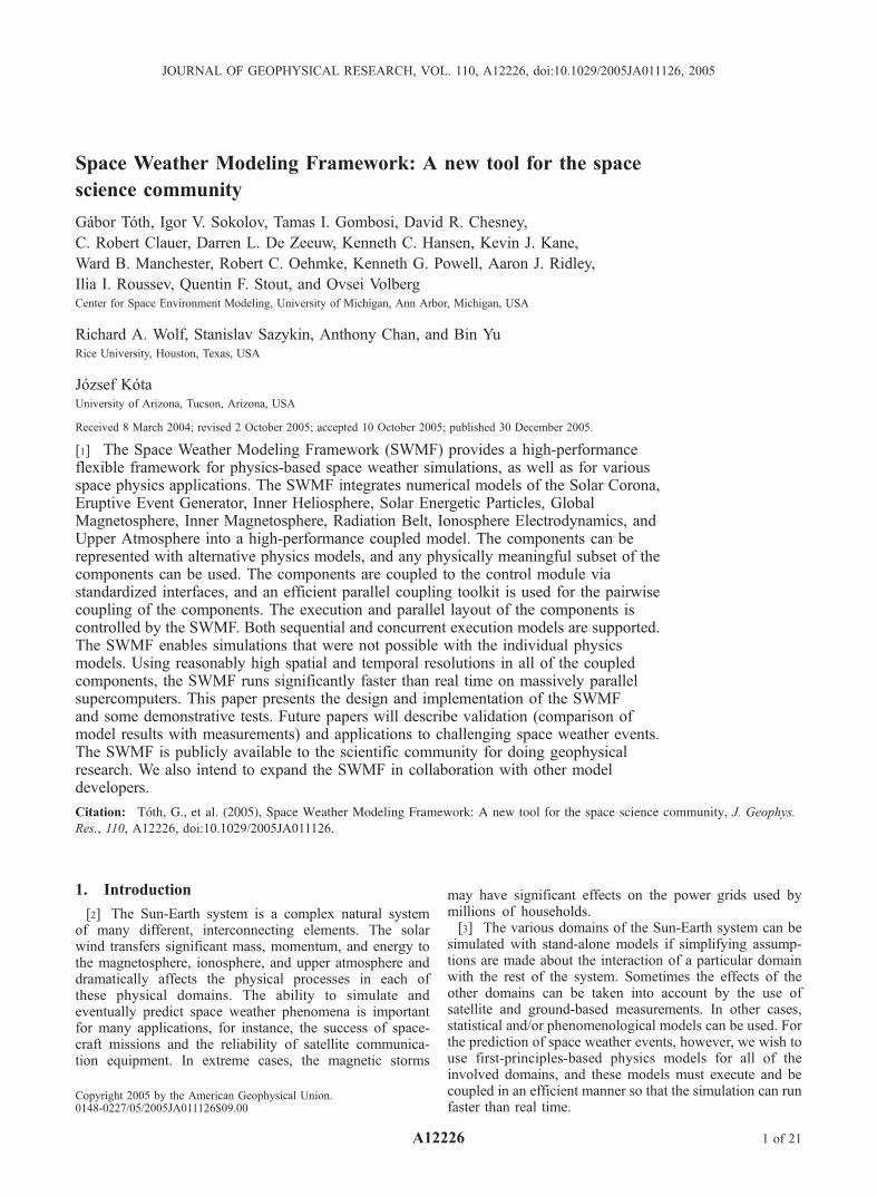
[8] The current version of the SWMF includes ninephysics domains ranging from the surface of the Sun tothe surface of a planet (usually the Earth). The nine physicsdomains are the following: (1) Solar Corona (SC),(2) Eruptive Event Generator (EE), (3) Inner Heliosphere(IH), (4) Solar Energetic Particles (SP), (5) GlobalMagnetosphere (GM), (6) Inner Magnetosphere (IM),(7) Radiation Belt (RB), (8) Ionosphere Electrodynamics(IE), (9) Upper Atmosphere (UA). The physics domainsdepicted in Figure 1 correspond to the components of theframework. Each component can have multiple versions. Acomponent version is based on a particular physics model,which is implemented by a particular physics module.[9] We note here that in the current version of the SWMF

the EE and SC domains are represented by one component.The reason is that there are a multitude of approaches bywhich an eruptive event can be generated, and each ap-proach has different but rather tight coupling with the solarcorona model. Since the SWMF is able to run with anysubset of the components, it is possible to combine anumber of domains into one component as long as onlyone of the combined domains is coupled to the rest of thecomponents. For example, the EE, SC, IH, and SP domainscould be represented by a single ‘‘super’’ IH componentbecause the only coupling required from this subset ofdomains is the coupling with the global magnetosphere.Similarly, the IE and UA domains can be represented with asingle ‘‘super’’ IE component, since (at least currently) theUA domain is only coupled directly to the IE domain.[10] A new domain can be added to the framework in two

different ways. One approach is to incorporate the newdomain into an existing component. For example, one mayadd a reconnection model to the GM component to betterrepresent the physics of the magnetic reconnection. Thisapproach will minimize the development work, but it resultsin a less flexible framework, since it will be difficult toreplace the reconnection model with alternatives, and it willnot be possible to use the same reconnection model withalternative versions of the GM component. To truly extendthe SWMF, one needs to define a new domain and add anew component to the framework. The SWMF has beenextended with new physics domains several times duringthe development process, and the sequence of steps to takeis described in the documentation.[11] While using a monolithic model to represent a large

subset of the components is a possibility, it is at odds withthe purpose of the framework, which aims to provide accessand control to the individual domains. Let us reiterate the

A12226 TOTH ET AL.: SPACE WEATHER MODELING FRAMEWORK

2 of 21

A12226

advantages of using components instead of a single mono-lithic code. Although it is possible to approximate thephysics from the surface of the Sun to the surface of theEarth with a single MHD code, there are many advantagesof dividing up the work into the SC, IH, and GM compo-nents. Each component may use slightly different equations,different coordinate systems, different grids, and differentnumerical schemes, which are optimized for the particularphysics domain. The components may have multiple ver-sions or can be replaced with measurements. For example,the Global Magnetosphere may be driven by the measure-ments of the ACE satellite instead of the IH component. Themultiple component approach results in more optimal rep-resentation of the physics domains and it allows a largenumber of combinations. All of these advantages make theframework more accurate, efficient, and versatile than amonolithic code.[12] Below we briefly describe all nine physics domains,

the typical coordinate systems, the equations to be solved,the boundary conditions, and the couplings with the otherdomains. A component is responsible for solving thedynamical equations in its domain, and it is also responsiblefor receiving and providing information as needed. Themost computationally challenging couplings are describedin more detail, since these present additional tasks to beaccomplished by the components.[13] Before going into the description of the individual

models, we provide a brief outline of the essential

couplings of the domains when all the components ofthe SWMF are used: The Eruptive Event generator iscoupled with the Solar Corona model only. The SolarCorona model drives the Inner Heliosphere model. Boththe SC and the IH models provide input to the SolarEnergetic Particles model. The Inner Heliosphere modeldrives the coupled system of the Global Magnetosphere,Inner Magnetosphere, Ionospheric Electrodynamics, andUpper Atmosphere models through the IH/GM interface.The Radiation Belt model receives information from theGM model only.

2.1. Solar Corona (SC)

[14] The Solar Corona domain extends from the lowcorona at �1 RS (solar radius) to approximately 24 RS.The physics of this domain is well approximated with theequations of magnetohydrodynamics; however, additionalsource terms are required to take into account gravity, theheating, and acceleration of the solar wind [Groth et al.,2000; Usmanov et al., 2000]. Alternative models mimic thecoronal heating by incorporating a variable adiabatic index[Wu et al., 1999] or solve for one extra equation thatdescribes the energy interchange between the solarwind plasma and the large-scale MHD turbulence [Roussevet al., 2003b]. The SC component can be in an inertial (e.g.,Heliographic Inertial (HGI)) frame or in a rotating (e.g.,Heliographic Rotating (HGR)) frame. In a rotating framethe inertial forces must be included.

Figure 1. The Space Weather Modeling Framework (SWMF) and its nine physics domains.


3 of 21

A12226

[15] The inner boundary of the SC component is drivenby the density, pressure, velocity, and magnetic field definedjust above the photosphere. The magnetic field may beobtained from synoptic magnetograms, or a simple dipole(possibly with a few higher-order terms) may be assumed.The boundary conditions for the temperature and massdensity at the Sun may vary with longitude and latitude toachieve the most realistic solar wind near the Sun and at1 AU. The velocity components at the inner boundaryshould maintain line-tying of the magnetic field. The flowat the outer boundary is usually superfast (faster than thefast magnetosonic speed of the plasma), so no informationis propagating inward. Sometimes, however, when a coronalmass ejection (CME) passes the boundary, the solar windspeed may become subfast for short periods of time. Duringsuch periods, the SC component needs to receive the outerboundary condition from the Inner Heliosphere.[16] The Solar Corona provides the plasma variables at

the inner boundary of the Inner Heliosphere. The innerboundary of the IH component does not have to coincidewith the outer boundary of the Solar Corona, i.e., the twodomains are allowed to overlap. Such an overlap is actuallynumerically advantageous when the flow becomes subfastfor a short time. The overlap can reduce reflections or othernumerical artifacts at the inner boundary of the IH, whichcould otherwise arise for subfast flow when the SC and IHcomponents use unaligned grids and different time steps.The Solar Corona also provides information to the SolarEnergetic Particle domain: the geometry of one or multiplefield lines and the plasma parameters along each field lineare provided to the SP component.

2.2. Eruptive Event Generator (EE)

[17] The EE domain is embedded in the Solar Corona,and it is restricted to the region of the eruptive event, whichis typically in the form of a coronal mass ejection (CME).To date, we lack good understanding of the actual physicalprocesses by which a CME is initiated, and it is still anactive field of research. One group of models [Forbes andIsenberg, 1991; Gibson and Low, 1998; Roussev et al.,2003a] assume that a magnetic flux rope exists prior to theeruption. Flux ropes may suddenly lose mechanical equi-librium and erupt due to foot-point motions [Wu et al.,2000], injection of magnetic helicity [Chen and Garren,1993], or draining of heavy prominence material [Low,2001]. Another group of models [Antiochos et al., 1999;Manchester, 2003; Roussev et al., 2004] relies on theexistence of sheared magnetic arcades, which becomeunstable and erupt once some critical state is reached. Herea flux rope is formed by reconnection between the oppositepolarity feet of the arcade during the eruption process.[18] The EE component can be represented as a boundary

condition for the SC component, or it can be a (nonlinear)perturbation of the SC solution. In short, the EE componentinteracts with the SC component only. Owing to themultitude of possibilities, the EE component is integratedinto the SC component in the current implementation of theSWMF. Multiple EE versions are possible, but all the EEversions belong to one SC version only.[19] We note that the eruptive event generator can be

regarded as a boundary condition or as a perturbation of theinitial conditions for the time accurate evolution of the solar

corona. The time accurate evolution itself follows thegoverning MHD equations with the source terms.

2.3. Inner Heliosphere (IH)

[20] The IH domain extends from around 20 solar radii allthe way to the planet. It does not have to cover a sphericalregion, it may be rectangular and asymmetric with respect tothe center of the Sun. The physics of this domain is wellapproximated with the equations of ideal MHD. The IHcomponent is usually in an inertial (e.g., HGI) frame.[21] The inner boundary conditions of the IH component

are obtained from the SC component or measurements. Theflow at the outer boundary of the IH component is alwayssuperfast (the interaction with the interstellar medium isoutside of the IH). The Inner Heliosphere provides the sameinformation to the SP component as the Solar Corona. TheIH component also provides the outer boundaries for the SCcomponent when the flow at the outer boundary of SC is notsuperfast. Finally, the Inner Heliosphere provides the up-stream boundary conditions for the Global Magnetosphere.The IH and GM domains overlap: the upstream boundary ofGM is typically at about 30 RE (Earth radii) from the Earthtoward the Sun, which is inside the IH domain.

2.4. Solar Energetic Particles (SP)

[22] The SP domain consists of one or more one dimen-sional field lines, which are assumed to advect with theplasma. The physics of this domain is responsible for theacceleration of the solar energetic particles along the fieldlines. There are various mathematical models that approx-imate this physical system. They include the effects ofacceleration and spatial diffusion and can be averaged[Sokolov et al., 2004] or nonaveraged [Kota and Jokipii,1999; J. Kota et al., Acceleration and Transport of SolarEnergetic Particles in a Simulated CME Environment,submitted to Astrophysical Journal, 2005, hereinafter re-ferred to as Kota et al., submitted manuscript, 2005] withrespect to pitch angle.[23] The geometry of the field line and the plasma

parameters along the field line are obtained from the SCand IH components. The boundary conditions can be zeroparticle flux at the ends of the field line(s). The SPcomponent does not currently provide information to othercomponents.

2.5. Global Magnetosphere (GM)

[24] The GM domain contains the bow shock, magneto-pause, and magnetotail of the planet. The GM domaintypically extends to about 30 RE on the dayside, hundredsof RE on the nightside, and 50 to 100 RE in the directionsorthogonal to the Sun-Earth line. The physics of this domainis approximated with the resistive MHD equations exceptnear the planet, where it overlaps with the Inner Magneto-sphere. The GM component typically uses Geocentric SolarMagnetic (GSM), Geocentric Solar Ecliptic (GSE), orpossibly Solar Magnetic (SM) coordinate system.[25] The upstream boundary conditions are obtained from

the IH component or from satellite measurements. At theother outer boundaries one can usually assume zero gradientfor the plasma variables, since these boundaries are farenough from the planet to have no significant effect on thedynamics near the planet. The inner boundary of the Global


4 of 21

A12226

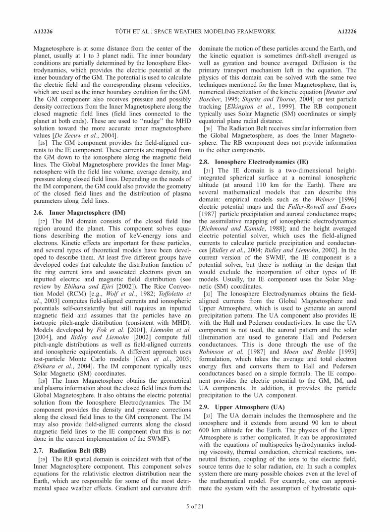
Magnetosphere is at some distance from the center of theplanet, usually at 1 to 3 planet radii. The inner boundaryconditions are partially determined by the Ionosphere Elec-trodynamics, which provides the electric potential at theinner boundary of the GM. The potential is used to calculatethe electric field and the corresponding plasma velocities,which are used as the inner boundary condition for the GM.The GM component also receives pressure and possiblydensity corrections from the Inner Magnetosphere along theclosed magnetic field lines (field lines connected to theplanet at both ends). These are used to ‘‘nudge’’ the MHDsolution toward the more accurate inner magnetospherevalues [De Zeeuw et al., 2004].[26] The GM component provides the field-aligned cur-

rents to the IE component. These currents are mapped fromthe GM down to the ionosphere along the magnetic fieldlines. The Global Magnetosphere provides the Inner Mag-netosphere with the field line volume, average density, andpressure along closed field lines. Depending on the needs ofthe IM component, the GM could also provide the geometryof the closed field lines and the distribution of plasmaparameters along field lines.

2.6. Inner Magnetosphere (IM)

[27] The IM domain consists of the closed field lineregion around the planet. This component solves equa-tions describing the motion of keV-energy ions andelectrons. Kinetic effects are important for these particles,and several types of theoretical models have been devel-oped to describe them. At least five different groups havedeveloped codes that calculate the distribution function ofthe ring current ions and associated electrons given aninputted electric and magnetic field distribution (seereview by Ebihara and Ejiri [2002]). The Rice Convec-tion Model (RCM) [e.g., Wolf et al., 1982; Toffoletto etal., 2003] computes field-aligned currents and ionosphericpotentials self-consistently but still requires an inputtedmagnetic field and assumes that the particles have anisotropic pitch-angle distribution (consistent with MHD).Models developed by Fok et al. [2001], Liemohn et al.[2004], and Ridley and Liemohn [2002] compute fullpitch-angle distributions as well as field-aligned currentsand ionospheric equipotentials. A different approach usestest-particle Monte Carlo models [Chen et al., 2003;Ebihara et al., 2004]. The IM component typically usesSolar Magnetic (SM) coordinates.[28] The Inner Magnetosphere obtains the geometrical

and plasma information about the closed field lines from theGlobal Magnetosphere. It also obtains the electric potentialsolution from the Ionosphere Electrodynamics. The IMcomponent provides the density and pressure correctionsalong the closed field lines to the GM component. The IMmay also provide field-aligned currents along the closedmagnetic field lines to the IE component (but this is notdone in the current implementation of the SWMF).

2.7. Radiation Belt (RB)

[29] The RB spatial domain is coincident with that of theInner Magnetosphere component. This component solvesequations for the relativistic electron distribution near theEarth, which are responsible for some of the most detri-mental space weather effects. Gradient and curvature drift

dominate the motion of these particles around the Earth, andthe kinetic equation is sometimes drift-shell averaged aswell as gyration and bounce averaged. Diffusion is theprimary transport mechanism left in the equation. Thephysics of this domain can be solved with the same twotechniques mentioned for the Inner Magnetosphere, that is,numerical discretization of the kinetic equation [Beutier andBoscher, 1995; Shprits and Thorne, 2004] or test particletracking [Elkington et al., 1999]. The RB componenttypically uses Solar Magnetic (SM) coordinates or simplyequatorial plane radial distance.[30] The Radiation Belt receives similar information from

the Global Magnetosphere, as does the Inner Magneto-sphere. The RB component does not provide informationto the other components.

2.8. Ionosphere Electrodynamics (IE)

[31] The IE domain is a two-dimensional height-integrated spherical surface at a nominal ionosphericaltitude (at around 110 km for the Earth). There areseveral mathematical models that can describe thisdomain: empirical models such as the Weimer [1996]electric potential maps and the Fuller-Rowell and Evans[1987] particle precipitation and auroral conductance maps;the assimilative mapping of ionospheric electrodynamics[Richmond and Kamide, 1988]; and the height averagedelectric potential solver, which uses the field-alignedcurrents to calculate particle precipitation and conductan-ces [Ridley et al., 2004; Ridley and Liemohn, 2002]. In thecurrent version of the SWMF, the IE component is apotential solver, but there is nothing in the design thatwould exclude the incorporation of other types of IEmodels. Usually, the IE component uses the Solar Mag-netic (SM) coordinates.[32] The Ionosphere Electrodynamics obtains the field-

aligned currents from the Global Magnetosphere andUpper Atmosphere, which is used to generate an auroralprecipitation pattern. The UA component also provides IEwith the Hall and Pedersen conductivities. In case the UAcomponent is not used, the auroral pattern and the solarillumination are used to generate Hall and Pedersenconductances. This is done through the use of theRobinson et al. [1987] and Moen and Brekke [1993]formulation, which takes the average and total electronenergy flux and converts them to Hall and Pedersenconductances based on a simple formula. The IE compo-nent provides the electric potential to the GM, IM, andUA components. In addition, it provides the particleprecipitation to the UA component.

2.9. Upper Atmosphere (UA)

[33] The UA domain includes the thermosphere and theionosphere and it extends from around 90 km to about600 km altitude for the Earth. The physics of the UpperAtmosphere is rather complicated. It can be approximatedwith the equations of multispecies hydrodynamics includ-ing viscosity, thermal conduction, chemical reactions, ion-neutral friction, coupling of the ions to the electric field,source terms due to solar radiation, etc. In such a complexsystem there are many possible choices even at the level ofthe mathematical model. For example, one can approxi-mate the system with the assumption of hydrostatic equi-


5 of 21

A12226

librium [Richmond et al., 1992] or use a compressiblehydrodynamic description [Ridley et al., 2005]. The UAcomponent is typically in a planet-centric rotating frame,i.e., the Geocentric (GEO) coordinate system for the Earth.[34] The lower and upper boundaries of the UA domain

are approximated with physically motivated boundaryconditions. The Upper Atmosphere obtains the electricpotential along the magnetic field lines and the particleprecipitation from the Ionosphere Electrodynamics. Thegradient of the potential provides the electric field, whichis used to drive the ion motion, while the auroralprecipitation is used to calculate ionization rates. TheUA component provides field-aligned currents and theHall and Pedersen conductivities to the IE component.The conductivities are calculated from the electron den-sity and integrated along field lines.

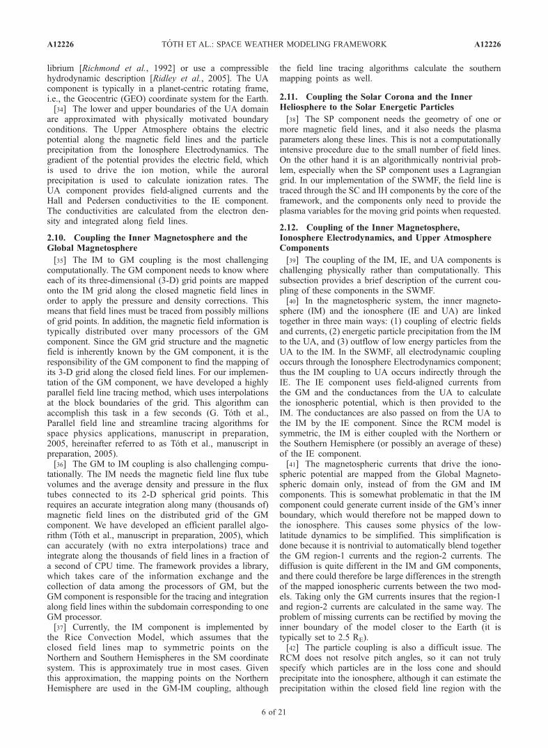
2.10. Coupling the Inner Magnetosphere and theGlobal Magnetosphere

[35] The IM to GM coupling is the most challengingcomputationally. The GM component needs to know whereeach of its three-dimensional (3-D) grid points are mappedonto the IM grid along the closed magnetic field lines inorder to apply the pressure and density corrections. Thismeans that field lines must be traced from possibly millionsof grid points. In addition, the magnetic field information istypically distributed over many processors of the GMcomponent. Since the GM grid structure and the magneticfield is inherently known by the GM component, it is theresponsibility of the GM component to find the mapping ofits 3-D grid along the closed field lines. For our implemen-tation of the GM component, we have developed a highlyparallel field line tracing method, which uses interpolationsat the block boundaries of the grid. This algorithm canaccomplish this task in a few seconds (G. Toth et al.,Parallel field line and streamline tracing algorithms forspace physics applications, manuscript in preparation,2005, hereinafter referred to as Toth et al., manuscript inpreparation, 2005).[36] The GM to IM coupling is also challenging compu-

tationally. The IM needs the magnetic field line flux tubevolumes and the average density and pressure in the fluxtubes connected to its 2-D spherical grid points. Thisrequires an accurate integration along many (thousands of)magnetic field lines on the distributed grid of the GMcomponent. We have developed an efficient parallel algo-rithm (Toth et al., manuscript in preparation, 2005), whichcan accurately (with no extra interpolations) trace andintegrate along the thousands of field lines in a fraction ofa second of CPU time. The framework provides a library,which takes care of the information exchange and thecollection of data among the processors of GM, but theGM component is responsible for the tracing and integrationalong field lines within the subdomain corresponding to oneGM processor.[37] Currently, the IM component is implemented by

the Rice Convection Model, which assumes that theclosed field lines map to symmetric points on theNorthern and Southern Hemispheres in the SM coordinatesystem. This is approximately true in most cases. Giventhis approximation, the mapping points on the NorthernHemisphere are used in the GM-IM coupling, although

the field line tracing algorithms calculate the southernmapping points as well.

2.11. Coupling the Solar Corona and the InnerHeliosphere to the Solar Energetic Particles

[38] The SP component needs the geometry of one ormore magnetic field lines, and it also needs the plasmaparameters along these lines. This is not a computationallyintensive procedure due to the small number of field lines.On the other hand it is an algorithmically nontrivial prob-lem, especially when the SP component uses a Lagrangiangrid. In our implementation of the SWMF, the field line istraced through the SC and IH components by the core of theframework, and the components only need to provide theplasma variables for the moving grid points when requested.

2.12. Coupling of the Inner Magnetosphere,Ionosphere Electrodynamics, and Upper AtmosphereComponents

[39] The coupling of the IM, IE, and UA components ischallenging physically rather than computationally. Thissubsection provides a brief description of the current cou-pling of these components in the SWMF.[40] In the magnetospheric system, the inner magneto-

sphere (IM) and the ionosphere (IE and UA) are linkedtogether in three main ways: (1) coupling of electric fieldsand currents, (2) energetic particle precipitation from the IMto the UA, and (3) outflow of low energy particles from theUA to the IM. In the SWMF, all electrodynamic couplingoccurs through the Ionosphere Electrodynamics component;thus the IM coupling to UA occurs indirectly through theIE. The IE component uses field-aligned currents fromthe GM and the conductances from the UA to calculatethe ionospheric potential, which is then provided to theIM. The conductances are also passed on from the UA tothe IM by the IE component. Since the RCM model issymmetric, the IM is either coupled with the Northern orthe Southern Hemisphere (or possibly an average of these)of the IE component.[41] The magnetospheric currents that drive the iono-

spheric potential are mapped from the Global Magneto-spheric domain only, instead of from the GM and IMcomponents. This is somewhat problematic in that the IMcomponent could generate current inside of the GM’s innerboundary, which would therefore not be mapped down tothe ionosphere. This causes some physics of the low-latitude dynamics to be simplified. This simplification isdone because it is nontrivial to automatically blend togetherthe GM region-1 currents and the region-2 currents. Thediffusion is quite different in the IM and GM components,and there could therefore be large differences in the strengthof the mapped ionospheric currents between the two mod-els. Taking only the GM currents insures that the region-1and region-2 currents are calculated in the same way. Theproblem of missing currents can be rectified by moving theinner boundary of the model closer to the Earth (it istypically set to 2.5 RE).[42] The particle coupling is also a difficult issue. The

RCM does not resolve pitch angles, so it can not trulyspecify which particles are in the loss cone and shouldprecipitate into the ionosphere, although it can estimate theprecipitation within the closed field line region with the


6 of 21

A12226

assumption of strong pitch-angle scattering. The SWMFcurrently uses an empirical relationship in the IE componentto estimate the precipitation based on the field-alignedcurrents obtained from the GM. This approach has theadvantage that the precipitation is calculated the sameway inside and outside the closed field line region. Theionospheric outflow is not included in the framework at thistime.[43] The IE-GM and the IE-UA couplings all use map-

pings along magnetic field lines. The IE-GM mapping usesan analytic formula assuming a tilted dipole field. The UA-IE coupling uses numerical integration along field lineseither based on a dipole or a more realistic field. Thetransformations between the coordinate systems (GSM forGM, SM for IE, and GEO for UA) and the mapping alongmagnetic dipole field lines are done with the libraryfunctions of the SWMF Infrastructure Layer (see the nextsection).

3. Architecture of the SWMF

[44] The SWMF provides a flexible and extensible soft-ware architecture for multicomponent physics-based space-weather simulations, as well as for various space physicsapplications. The main SWMF design goals are to(1) incorporate computational physics modules with onlymodest modification, (2) achieve good parallel performance,and (3) make the SWMF as versatile as possible. Thesedesign goals are orthogonal to each other, and the actualdesign represents a tradeoff. One can minimize the changesin the physics modules at the expense of performance andflexibility, or one may maximize software reuse and inte-gration at the expense of the other design goals. The SWMFdesign focuses on achieving good performance, while theversatility of the SWMF and the minimization of codechange are taken into consideration as much as possible.

The initial investment into the integration of the physicsmodules pays off in the flexibility, usability, and the perfor-mance of the SWMF. In our experience, it takes about2 weeks of work by one or two people to integrate a newphysics module into the framework. Typically, a fewhundred lines of new code need to be written, but thisstrongly depends on the number and complexity of thecouplings. The integration includes verification that thecomponent still functions correctly, and it sends and receivesdata from other components as designed. Fine tuning thecouplings and improving the physics of the combined frame-workmay takemore time, but this is related to the complexityof the physics rather than the software development.[45] One of the most important features of the SWMF is

that it can incorporate different computational physicsmodules to model different domains of the Sun-Earthsystem. Each module for a particular domain can bereplaced with alternatives, and one can use only a subsetof the modules if desired.

3.1. Design Challenges

[46] There are several problems known a priori, whichneed to be solved so that the heterogeneous computationalmodels of the different domains of the Sun-Earth system canproperly interoperate. An incomplete list of these problemsis as follows: (1) There are serial and parallel models; (2) Anindividual model is usually developed for stand-alone exe-cution; (3) Input/output operations do not take into accountpotential conflicts with other models; (4) The majority ofmodels are not written in object oriented style, which meansthat data and procedure name conflicts can easily occur;(5) Models often do not have checkpoint and restart capa-bilities; (6) The efficient coupling of any arbitrary pair ofparallel applications, each of them having its own gridstructure and data decomposition, is not easily achieved.Some of the problems, like name space and I/O unit conflicts,can be avoided if the physics components are compiled intoindividual executable programs. However, coupling multipleexecutables via the Message Passing Interface (MPI) is notgenerally supported on our target platforms. For this reasonthe SWMF has been designed to compile and run as asingle executable, and we have developed automatedsolutions to resolve procedure name and I/O unit numberconflicts. The design does not exclude multiple execut-ables, in fact the SWMF can be compiled to include only asubset of the components. In principle one could rundifferent configurations of the SWMF together, but thiswould be more complicated than using a single executable.[47] The interaction of the (replaceable) physics modules

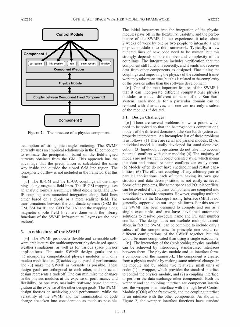
can be achieved by introducing standardized interfacesbetween them. The physics module and its interface formsa component of the framework. The component is createdfrom a physics module by making some minimal changes inthe module and by adding two relatively small units ofcode: (1) a wrapper, which provides the standard interfaceto control the physics module, and (2) a coupling interface,to perform the data exchange other components. Both thewrapper and the coupling interface are component interfa-ces: the wrapper is an interface with the high-level ControlModule (CON) of the framework, and the coupling interfaceis an interface with the other components. As shown inFigure 2, the wrapper interface functions have standard

Figure 2. The structure of a physics component.


7 of 21

A12226

names, which makes swapping between various versions ofa component possible. The data exchange between thecomponents includes all the necessary unit conversions,mapping, coordinate transformation, and interpolations.Both the wrapper and the coupling interface are constructedfrom the building blocks provided by the framework.

3.2. Requirements for Physics Modules

[48] The physics modules must comply with a minimumset of requirements before they are transformed into acomponent. (1) The parallelization mechanism (if any)should employ the MPI standard and the physics moduleshould be able to use an arbitrary MPI communicator;(2) The module needs to be compiled as a library that couldbe linked to another executable; (3) The module should readinput from and write output to files that are in a subdirectoryunique for the component; (4) A module should be imple-mented in Fortran 77 and/or Fortran 90; (5) The moduleshould be portable to a specific combination of platformsand compilers, which include Linux clusters and NASAsupercomputers; (6) The stand-alone module must success-fully run a model test suite provided by the model developeron all the required platform/compiler combinations; (7) Amodule should be supplied with appropriate documentation.The first three requirements directly address the problemslisted in the previous subsection, while the rest make theintegration work into the SWMF possible and ensure theportability of the SWMF. Since the core of the SWMF iswritten in Fortran 90, there is no need to solve the issuesthat arise when a software is written in multiple languages.

3.3. Component Wrapper and Coupler

[49] The SWMF requirements for a component are de-fined in terms of a set of methods implemented in thecomponent interface, i.e., the wrapper and the couplers. Themethods enable the component to perform the followingtasks: (1) provide version name and number to the ControlModule; (2) accept parameters for parallel configuration;(3) accept and check input parameters obtained from theControl Module; (4) provide grid description to the ControlModule; (5) initialize for session execution and read restartfiles if necessary; (6) execute one time step that cannotexceed a specified simulation time; (7) receive and providedata to another component via an appropriate coupler;(8) write its state into a restart file when requested;(9) finalize at the end of the execution. The structure of acomponent and its interaction with the Control Module(CON) and another component are illustrated in Figure 2.

3.4. Layered Architecture

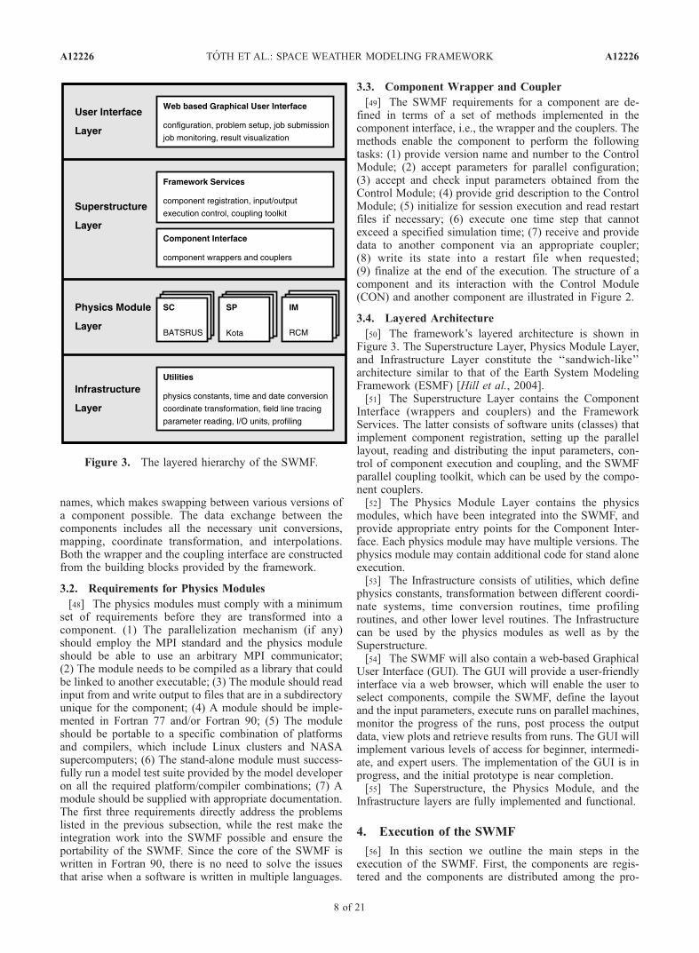
[50] The framework’s layered architecture is shown inFigure 3. The Superstructure Layer, Physics Module Layer,and Infrastructure Layer constitute the ‘‘sandwich-like’’architecture similar to that of the Earth System ModelingFramework (ESMF) [Hill et al., 2004].[51] The Superstructure Layer contains the Component

Interface (wrappers and couplers) and the FrameworkServices. The latter consists of software units (classes) thatimplement component registration, setting up the parallellayout, reading and distributing the input parameters, con-trol of component execution and coupling, and the SWMFparallel coupling toolkit, which can be used by the compo-nent couplers.[52] The Physics Module Layer contains the physics

modules, which have been integrated into the SWMF, andprovide appropriate entry points for the Component Inter-face. Each physics module may have multiple versions. Thephysics module may contain additional code for stand aloneexecution.[53] The Infrastructure consists of utilities, which define

physics constants, transformation between different coordi-nate systems, time conversion routines, time profilingroutines, and other lower level routines. The Infrastructurecan be used by the physics modules as well as by theSuperstructure.[54] The SWMF will also contain a web-based Graphical

User Interface (GUI). The GUI will provide a user-friendlyinterface via a web browser, which will enable the user toselect components, compile the SWMF, define the layoutand the input parameters, execute runs on parallel machines,monitor the progress of the runs, post process the outputdata, view plots and retrieve results from runs. The GUI willimplement various levels of access for beginner, intermedi-ate, and expert users. The implementation of the GUI is inprogress, and the initial prototype is near completion.[55] The Superstructure, the Physics Module, and the

Infrastructure layers are fully implemented and functional.

4. Execution of the SWMF

[56] In this section we outline the main steps in theexecution of the SWMF. First, the components are regis-tered and the components are distributed among the pro-

Figure 3. The layered hierarchy of the SWMF.


8 of 21

A12226

cessors according to the requested layout. Next, the inputparameters are read and transferred to the components. Theexecution of the components starts after the components areinitialized and coupled for the first time. During the execu-tion the components are coupled and restart information issaved according to a predetermined schedule. At the end ofthe run the components are finalized. The following sub-sections provide more detail about these steps.

4.1. Registration and Layout of Components

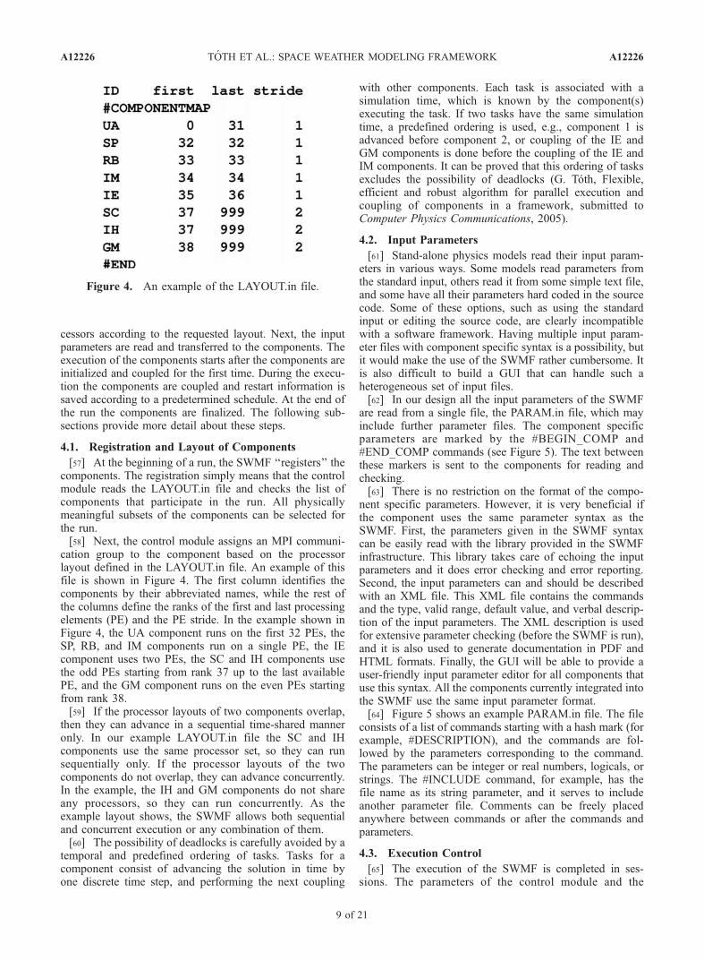
[57] At the beginning of a run, the SWMF ‘‘registers’’ thecomponents. The registration simply means that the controlmodule reads the LAYOUT.in file and checks the list ofcomponents that participate in the run. All physicallymeaningful subsets of the components can be selected forthe run.[58] Next, the control module assigns an MPI communi-

cation group to the component based on the processorlayout defined in the LAYOUT.in file. An example of thisfile is shown in Figure 4. The first column identifies thecomponents by their abbreviated names, while the rest ofthe columns define the ranks of the first and last processingelements (PE) and the PE stride. In the example shown inFigure 4, the UA component runs on the first 32 PEs, theSP, RB, and IM components run on a single PE, the IEcomponent uses two PEs, the SC and IH components usethe odd PEs starting from rank 37 up to the last availablePE, and the GM component runs on the even PEs startingfrom rank 38.[59] If the processor layouts of two components overlap,

then they can advance in a sequential time-shared manneronly. In our example LAYOUT.in file the SC and IHcomponents use the same processor set, so they can runsequentially only. If the processor layouts of the twocomponents do not overlap, they can advance concurrently.In the example, the IH and GM components do not shareany processors, so they can run concurrently. As theexample layout shows, the SWMF allows both sequentialand concurrent execution or any combination of them.[60] The possibility of deadlocks is carefully avoided by a

temporal and predefined ordering of tasks. Tasks for acomponent consist of advancing the solution in time byone discrete time step, and performing the next coupling

with other components. Each task is associated with asimulation time, which is known by the component(s)executing the task. If two tasks have the same simulationtime, a predefined ordering is used, e.g., component 1 isadvanced before component 2, or coupling of the IE andGM components is done before the coupling of the IE andIM components. It can be proved that this ordering of tasksexcludes the possibility of deadlocks (G. Toth, Flexible,efficient and robust algorithm for parallel execution andcoupling of components in a framework, submitted toComputer Physics Communications, 2005).

4.2. Input Parameters

[61] Stand-alone physics models read their input param-eters in various ways. Some models read parameters fromthe standard input, others read it from some simple text file,and some have all their parameters hard coded in the sourcecode. Some of these options, such as using the standardinput or editing the source code, are clearly incompatiblewith a software framework. Having multiple input param-eter files with component specific syntax is a possibility, butit would make the use of the SWMF rather cumbersome. Itis also difficult to build a GUI that can handle such aheterogeneous set of input files.[62] In our design all the input parameters of the SWMF

are read from a single file, the PARAM.in file, which mayinclude further parameter files. The component specificparameters are marked by the #BEGIN_COMP and#END_COMP commands (see Figure 5). The text betweenthese markers is sent to the components for reading andchecking.[63] There is no restriction on the format of the compo-

nent specific parameters. However, it is very beneficial ifthe component uses the same parameter syntax as theSWMF. First, the parameters given in the SWMF syntaxcan be easily read with the library provided in the SWMFinfrastructure. This library takes care of echoing the inputparameters and it does error checking and error reporting.Second, the input parameters can and should be describedwith an XML file. This XML file contains the commandsand the type, valid range, default value, and verbal descrip-tion of the input parameters. The XML description is usedfor extensive parameter checking (before the SWMF is run),and it is also used to generate documentation in PDF andHTML formats. Finally, the GUI will be able to provide auser-friendly input parameter editor for all components thatuse this syntax. All the components currently integrated intothe SWMF use the same input parameter format.[64] Figure 5 shows an example PARAM.in file. The file

consists of a list of commands starting with a hash mark (forexample, #DESCRIPTION), and the commands are fol-lowed by the parameters corresponding to the command.The parameters can be integer or real numbers, logicals, orstrings. The #INCLUDE command, for example, has thefile name as its string parameter, and it serves to includeanother parameter file. Comments can be freely placedanywhere between commands or after the commands andparameters.

4.3. Execution Control

[65] The execution of the SWMF is completed in ses-sions. The parameters of the control module and the

Figure 4. An example of the LAYOUT.in file.


9 of 21

A12226

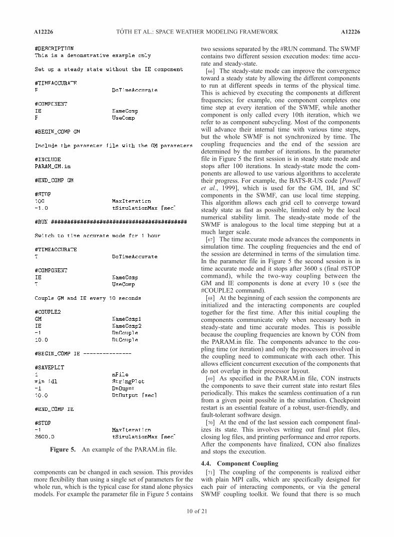
components can be changed in each session. This providesmore flexibility than using a single set of parameters for thewhole run, which is the typical case for stand alone physicsmodels. For example the parameter file in Figure 5 contains

two sessions separated by the #RUN command. The SWMFcontains two different session execution modes: time accu-rate and steady-state.[66] The steady-state mode can improve the convergence

toward a steady state by allowing the different componentsto run at different speeds in terms of the physical time.This is achieved by executing the components at differentfrequencies; for example, one component completes onetime step at every iteration of the SWMF, while anothercomponent is only called every 10th iteration, which werefer to as component subcycling. Most of the componentswill advance their internal time with various time steps,but the whole SWMF is not synchronized by time. Thecoupling frequencies and the end of the session aredetermined by the number of iterations. In the parameterfile in Figure 5 the first session is in steady state mode andstops after 100 iterations. In steady-state mode the com-ponents are allowed to use various algorithms to acceleratetheir progress. For example, the BATS-R-US code [Powellet al., 1999], which is used for the GM, IH, and SCcomponents in the SWMF, can use local time stepping.This algorithm allows each grid cell to converge towardsteady state as fast as possible, limited only by the localnumerical stability limit. The steady-state mode of theSWMF is analogous to the local time stepping but at amuch larger scale.[67] The time accurate mode advances the components in

simulation time. The coupling frequencies and the end ofthe session are determined in terms of the simulation time.In the parameter file in Figure 5 the second session is intime accurate mode and it stops after 3600 s (final #STOPcommand), while the two-way coupling between theGM and IE components is done at every 10 s (see the#COUPLE2 command).[68] At the beginning of each session the components are

initialized and the interacting components are coupledtogether for the first time. After this initial coupling thecomponents communicate only when necessary both insteady-state and time accurate modes. This is possiblebecause the coupling frequencies are known by CON fromthe PARAM.in file. The components advance to the cou-pling time (or iteration) and only the processors involved inthe coupling need to communicate with each other. Thisallows efficient concurrent execution of the components thatdo not overlap in their processor layout.[69] As specified in the PARAM.in file, CON instructs

the components to save their current state into restart filesperiodically. This makes the seamless continuation of a runfrom a given point possible in the simulation. Checkpointrestart is an essential feature of a robust, user-friendly, andfault-tolerant software design.[70] At the end of the last session each component final-

izes its state. This involves writing out final plot files,closing log files, and printing performance and error reports.After the components have finalized, CON also finalizesand stops the execution.

4.4. Component Coupling

[71] The coupling of the components is realized eitherwith plain MPI calls, which are specifically designed foreach pair of interacting components, or via the generalSWMF coupling toolkit. We found that there is so much

Figure 5. An example of the PARAM.in file.


10 of 21

A12226

variation between the physics and numerics of the couplingsthat it is not useful to make the couplings conform withsome abstract general coupler. The only general restrictionis that the data sent between the two components must be inSI units. The coupler must ensure that the data is correctlytransformed between the two components, but this isindividually achieved for each pairwise coupling.[72] Even the plain MPI couplers use some of the

SWMF infrastructure. A one-way coupler between twocomponents is built from three pieces: the get methodin the interface of the providing component, the putmethod in the interface of the receiving component, andthe data exchange in the control module, which containsthe allocation of the data buffers and all the requiredMPI communication calls. By breaking the coupler intopieces, each piece becomes simpler: the get and putmethods are very specific to the physics module but donot contain communication. The data exchange is specificfor the components but not too sensitive about whichcomponent version is used. The buffer size or thecoordinate transformations can use the grid descriptorsprovided by the components. The get method performsthe interpolations to the requested location, while the putmethod is usually a simple setting of the variables at therequested grid locations. The data exchange performs theMPI communication, which is often between the rootCPUs of the two components. This type of coupling isused when the interpolation and the communicationpatterns are relatively simple, for example when twoserial models with simple structured grids are coupled.For more complex cases the use of the SWMF parallelcoupling toolkit is preferred.[73] The couplings using the SWMF parallel coupling

toolkit can couple components based on the following typesof distributed grids: (1) 2-D or 3-D Cartesian or sphericalblock adaptive grid or (2) 1-D, 2-D, or 3-D structured grid.Structured grids include uniform and nonuniform sphericaland Cartesian grids.[74] The SWMF coupling toolkit obtains the grid descrip-

tors from the components at the beginning of the run. Thegrid descriptor defines the geometry and parallel decompo-sition of the grid. At the time of coupling the receivingcomponent requests a number of data values at specifiedlocations of the receiving grid (for example, all grid pointsat one of the boundaries). The geometric locations aretransformed, sometimes mapped, to the grid of the providercomponent by the coupling toolkit. On the basis of the griddescriptor of the provider component, the toolkit interpo-lates the data values to the requested locations and sendsthem to the requesting component. The toolkit providessecond order linear, bilinear, and trilinear interpolationschemes which work for all the supported grid types. Ifnecessary, the model can also use its own interpolationmethod in form of a subroutine, which is passed as anargument to the toolkit methods. The interpolation weightsand the MPI communication patterns are calculated inadvance and saved into a ‘‘router’’ for sake of efficiency.The router is reused in subsequent couplings. The routersare updated only if one of the grids has changed (e.g., due togrid adaptation) or when the mapping between the twocomponents has changed (e.g., due to the rotation of onegrid relative to the other).

[75] An interesting problem arises when the receivingcomponent uses an adaptive grid. If the receiving componentadapts its grid between two couplings, it may be difficult toget the coupling information for the newly created gridpoints. In this case it is useful to introduce an intermediategrid. The intermediate grid is usually a simple structured gridcovering the region where data is transferred, and it isreplicated on all the processors of the receiving component.The intermediate grid should have a sufficiently high reso-lution to keep the coupling accurate, but it should not behuge, otherwise the storage and the data transfer time maybecome a problem. The coupling with an intermediate gridconsists of the following steps: (1) The providing componentinterpolates data from its own grid to the intermediate grid.(2) The intermediate grid is collected and sent to all PEs ofthe receiving component. (3) The receiving componentinterpolates data from the intermediate grid to its adaptivegrid as needed. Often the first step is a trivial mappingbecause the intermediate grid is identical with (or a part of)the grid of the providing component. Both the plain MPI andthe toolkit based couplers can use an intermediate grid.

5. Component Versions

[76] The current version of the SWMF includes thefollowing component versions:[77] 1. The Solar Corona, Inner Heliosphere, and Global

Magnetosphere components are based on the University ofMichigan’s BATS-R-US code [Powell et al., 1999]. The SCcomponent uses the physical model of Roussev et al.[2003b], which incorporates magnetogram measurementsto specify the realistic boundary conditions for the potentialmagnetic field at the Sun. The highly parallel BATS-R-UScodeusesa3-Dblock-adaptiveCartesiangrid,high-resolutionshock capturing schemes, and explicit and/or implicittime stepping (G. Toth et al., A parallel explicit/implicittime stepping scheme on block-adaptive grids, submitted toJournal of Computational Physics, 2005, hereinafter referredto as Toth et al., submitted manuscript, 2005).[78] 2. The Eruptive Event Generator is implemented as

part of the SC/BATS-R-US component. There are twoversions: One superposes the Gibson and Low [Gibson andLow, 1998] magnetic flux rope to the background solar windsolution. The other version imposes converging and shearedvelocity field at the inner boundary [Roussev et al., 2004].Both versions were developed at the University of Michigan.[79] 3. The Solar Energetic Particles component has two

serial versions. The first is J. Kota’s SEP model (Kota et al.,submitted manuscript, 2005), which uses an operator splitimplicit scheme in one spatial, one pitch angle, and onemomentum dimension. This model has been developed atthe University of Arizona. The second component version isthe Field Line Advection Model for Particle Acceleration(FLAMPA) [Sokolov et al., 2004] using an explicit shockcapturing scheme in one spatial and one particle momentumdimension. This model has been developed at the Universityof Michigan.[80] 4. The Inner Magnetosphere component is the Rice

Convection Model (RCM) [Wolf et al., 1982; De Zeeuw etal., 2004] developed at Rice University. This serial moduleuses an explicit advection scheme on a 2-D nonuniformspherical grid.


11 of 21

A12226

[81] 5. The Radiation Belt component is the serial RiceRadiation Belt Model (RRBM) recently developed at RiceUniversity. It solves an adiabatic transformation of phasespace density on a 2-D nonuniform spherical grid. Althoughthe RRBM model is fully coupled and it runs, it is not yetfully functional.[82] 6. The Ionosphere Electrodynamics component is a

2-D spherical electric potential solver developed at theUniversity of Michigan [Ridley et al., 2004; Ridley andLiemohn, 2002]. It can run on one or two processors sincethe Northern and Southern Hemispheres can be solved inparallel.[83] 7. The Upper Atmosphere component is implemented

by two versions of the Global Ionosphere ThermosphereModel, GITM and GITM2 (A. J. Ridley et al., The GlobalIonosphere-Thermosphere Model, submitted to Journal ofAtmospheric and Solar-Terrestrial Physics, 2005). Bothversions have been recently developed at the Universityof Michigan as fully parallel 3-D spherical models. Theyuse different explicit upwind schemes for the advectionand GITM2 uses implicit time integration for the stiffsource terms.

6. Test Simulations

[84] We present results of two test simulations that involveall the components of the SWMF. The first simulation is usedas a comprehensive test for the framework, and it also serves

as a benchmark for its performance. This test illustrates thatthe SWMF with all components can run faster than real timewith reasonable spatial and temporal resolution. The SWMFcould be run in this now-casting mode using observed data.[85] The second test demonstrates how the eruption and

propagation of a single CME can be modeled with theSWMF. At the beginning of the run only the SC and IHcomponents are used. When the CME gets close to theEarth, the SC component can be ‘‘switched off’’ andthe GM, IM, IE, and UA components are ‘‘switched on.’’The GM component is initialized in a steady state modeusing the solar wind data obtained from the IH component.Since the SC and GM components are the most expensive,this strategy allows to run the SWMF about two times fasterthan with all the components. Alternatively, finer grids canbe used and still run faster than real time. We did the latterin the second test, i.e., the resolution in the SC and IHcomponents is increased to better follow the CME.[86] It should be emphasized that neither of these tests try

to model an actual space weather event, although we usereal magnetometer data to obtain the steady state solar windconditions. Our intention here is to demonstrate the use ofthe SWMF. Modeling and analyzing actual events will bedone in future papers.

6.1. Performance Test With All Components

[87] We present performance results of a test simulationthat involves all components of the SWMF. This simulation

Table 1. Spatial and Temporal Resolutions in the Test Run

Component Version Number of Cells Smallest Cell Variable/Cell Time Step

IH BATSRUS 2,500,000 1 RS 8 60.0 sSC BATSRUS 1,400,000 1/40 RS 9 0.4 sGM BATSRUS 1,300,000 1/4 RE 8 4.0 sUA GITM 64,800 5� � 5� � 2 km 30 10.0 sIE Ridley 33,000 1.4� � 1.4� 1 —SP Kota 10,000 0.1 RS � 10� 150 variesIM RCM 3,800 7.5� � 0.5� 150 5.0 sRB RRBM 3,800 7.5� � 0.5� 1 60.0 s

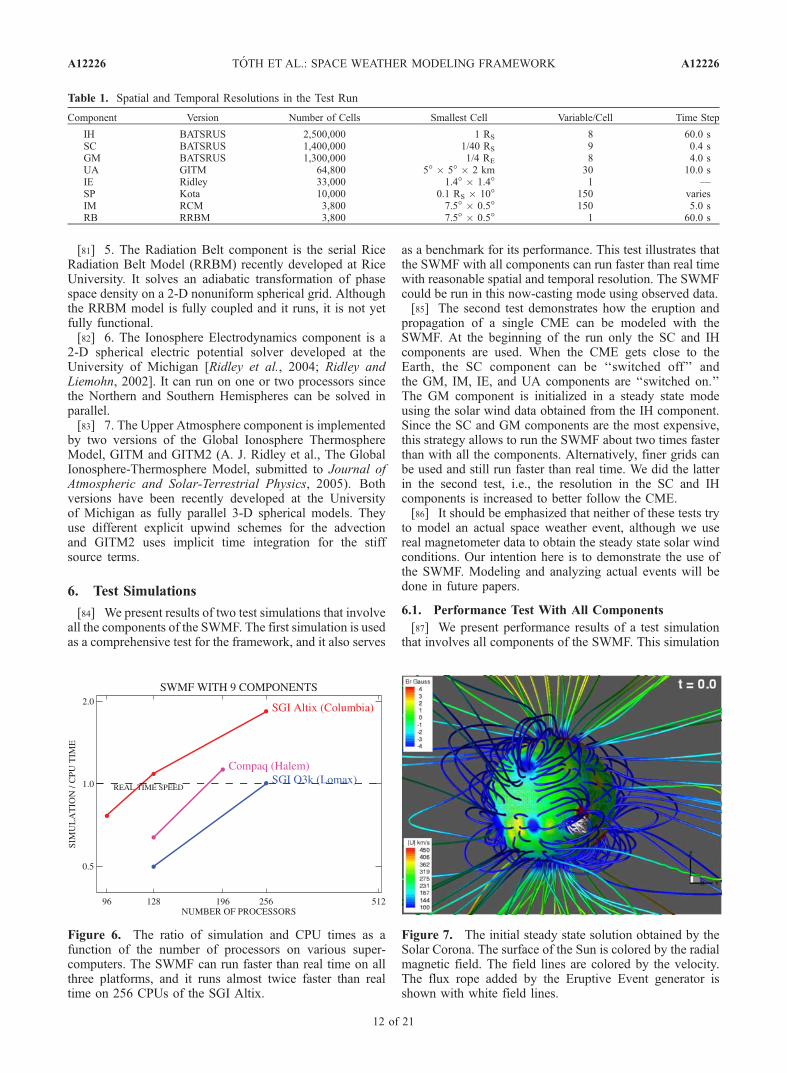
Figure 6. The ratio of simulation and CPU times as afunction of the number of processors on various super-computers. The SWMF can run faster than real time on allthree platforms, and it runs almost twice faster than realtime on 256 CPUs of the SGI Altix.

Figure 7. The initial steady state solution obtained by theSolar Corona. The surface of the Sun is colored by the radialmagnetic field. The field lines are colored by the velocity.The flux rope added by the Eruptive Event generator isshown with white field lines.


12 of 21

A12226

is used as a comprehensive test for the framework, and italso serves as a benchmark for its performance. Thesimulation grids of all the components have reasonablyhigh resolutions and the time steps and coupling frequenciesare all suitable to model space weather. Table 1 contains thegrid size, the number of state variables per grid cell, and thetime step information about all the components. It isinteresting to note that the time step in the SC component

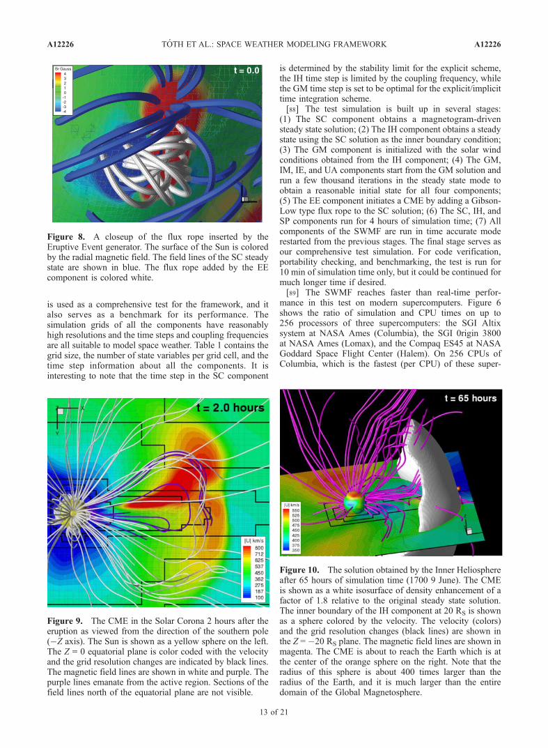
is determined by the stability limit for the explicit scheme,the IH time step is limited by the coupling frequency, whilethe GM time step is set to be optimal for the explicit/implicittime integration scheme.[88] The test simulation is built up in several stages:

(1) The SC component obtains a magnetogram-drivensteady state solution; (2) The IH component obtains a steadystate using the SC solution as the inner boundary condition;(3) The GM component is initialized with the solar windconditions obtained from the IH component; (4) The GM,IM, IE, and UA components start from the GM solution andrun a few thousand iterations in the steady state mode toobtain a reasonable initial state for all four components;(5) The EE component initiates a CME by adding a Gibson-Low type flux rope to the SC solution; (6) The SC, IH, andSP components run for 4 hours of simulation time; (7) Allcomponents of the SWMF are run in time accurate moderestarted from the previous stages. The final stage serves asour comprehensive test simulation. For code verification,portability checking, and benchmarking, the test is run for10 min of simulation time only, but it could be continued formuch longer time if desired.[89] The SWMF reaches faster than real-time perfor-

mance in this test on modern supercomputers. Figure 6shows the ratio of simulation and CPU times on up to256 processors of three supercomputers: the SGI Altixsystem at NASA Ames (Columbia), the SGI 0rigin 3800at NASA Ames (Lomax), and the Compaq ES45 at NASAGoddard Space Flight Center (Halem). On 256 CPUs ofColumbia, which is the fastest (per CPU) of these super-

Figure 8. A closeup of the flux rope inserted by theEruptive Event generator. The surface of the Sun is coloredby the radial magnetic field. The field lines of the SC steadystate are shown in blue. The flux rope added by the EEcomponent is colored white.

Figure 9. The CME in the Solar Corona 2 hours after theeruption as viewed from the direction of the southern pole(�Z axis). The Sun is shown as a yellow sphere on the left.The Z = 0 equatorial plane is color coded with the velocityand the grid resolution changes are indicated by black lines.The magnetic field lines are shown in white and purple. Thepurple lines emanate from the active region. Sections of thefield lines north of the equatorial plane are not visible.

Figure 10. The solution obtained by the Inner Heliosphereafter 65 hours of simulation time (1700 9 June). The CMEis shown as a white isosurface of density enhancement of afactor of 1.8 relative to the original steady state solution.The inner boundary of the IH component at 20 RS is shownas a sphere colored by the velocity. The velocity (colors)and the grid resolution changes (black lines) are shown inthe Z = �20 RS plane. The magnetic field lines are shown inmagenta. The CME is about to reach the Earth which is atthe center of the orange sphere on the right. Note that theradius of this sphere is about 400 times larger than theradius of the Earth, and it is much larger than the entiredomain of the Global Magnetosphere.


13 of 21

A12226

computers, the SWMF can run almost twice as fast as realtime. We emphasize that this speed is achieved withreasonable spatial and temporal resolution: the componentsuse about 47 million state variables in the discretizedphysics domains![90] There are several design and algorithmic choices

that make this performance possible. The concurrentexecution of the components allows good scaling up toa large number of CPUs. Even if the components do notscale perfectly to hundreds of CPUs, the whole SWMFcan because the components can use independent sets ofCPUs and they can progress concurrently. It is alsoimportant that the SWMF allows the overlap of the

component layouts, since the Inner Heliosphere runsmuch faster (due to the large time steps) than the othercomputationally expensive components. Still the IH needsa lot of CPUs for its large grid and the correspondingmemory requirements. In the time accurate simulationsthe SC and IH components use the same set of processors,otherwise all the components run concurrently on an optimalnumber of CPUs for the given component (see the processorlayout in Figure 4).[91] Another key to achieving this speed is that there are

three components to represent the Solar Corona, InnerHeliosphere, and Global Magnetosphere. Each componentuses the optimal grid and time stepping scheme in each

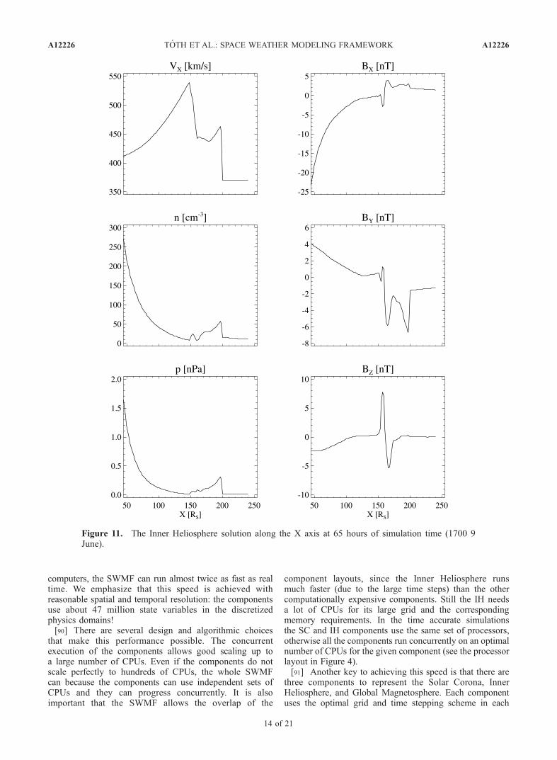
Figure 11. The Inner Heliosphere solution along the X axis at 65 hours of simulation time (1700 9June).


14 of 21

A12226

domain. The Solar Corona uses explicit time stepping withsmall 0.4 s time steps on a fine but relatively small grid. TheInner Heliosphere uses much larger 60 s time steps on itslarge but much coarser grid. Finally, the Global Magneto-sphere uses an efficient explicit/implicit time steppingscheme (Toth et al., submitted manuscript, 2005) on its finegrid, so the time step is not limited by the numericalstability condition. The optimal performance is achievedwith 4 s time steps, which speeds up the GM component byabout a factor of 30 relative to an explicit scheme.[92] The efficient coupling of the Global Magnetosphere

with the Inner Magnetosphere is also crucial in achievingfaster than real-time performance. The two components arecoupled every 40 s of simulation time and each couplinginvolves the mapping of the 1.3 million GM grid cellcenters to the IM grid along the dynamically changingmagnetic field lines. Owing to the efficient parallel field

line tracing algorithm (Toth et al., manuscript in prepara-tion, 2005) each coupling takes only a couple of seconds.

6.2. Generation and Propagation of a CME

[93] This simulation is built up in a similar manner as theprevious test, but this time the CME is propagated fromthe solar corona to the magnetosphere of the Earth. Thefollowing stages are used: (1) The SC component obtains amagnetogram driven steady state solution; (2) The IHcomponent obtains a steady state using the SC solution asthe inner boundary condition; (3) The GM component isinitialized with the solar wind conditions obtained from theIH component; (4) The EE component initiates a CME byadding a Gibson-Low type flux rope to the SC solution;(5) The SC and IH components run until the CME gets closeto the Earth; (6) The IH, GM, IM, IE, and UA componentsstart from the IH and GM solutions and the CME is

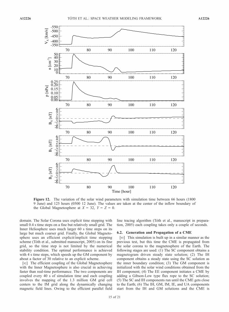
Figure 12. The variation of the solar wind parameters with simulation time between 66 hours (18009 June) and 125 hours (0500 12 June). The values are taken at the center of the inflow boundary ofthe Global Magnetosphere at X = 32, Y = Z = 0.


15 of 21

A12226

propagated through the magnetosphere. The time accurateruns in stages 5 and 6 are the computationally mostexpensive. In stage 5 the CME is propagating from theSC to the IH component, so only these two components arerun. In stage 6 the CME propagates from the IH to the GMcomponent and it effects all the other components near theEarth, but there is no need to run the SC component in thisstage. This partitioning of the simulation saves significantcomputational resources so that higher-resolution grids canbe used in the SC and IH components. The simulationstill progresses about two times faster than real time on256 CPUs of the SGI Altix supercomputer Columbia.[94] The SC grid is refined to 1/20 RS resolution out to

10 RS along the path of the CME, and a 1/4 RS resolution ismaintained along the Sun-Earth axis in the IH grid (see thegrid resolution boundaries in Figures 9 and 10). The refine-ments increase the number of grid cells to 2.5 million and8.2 million in the SC and IH components, respectively(compare with 1.4 and 2.5 million cells in the performancetest). The finer grid results in a better-resolved CME.[95] Figure 7 shows the magnetogram-based steady state

solution in the Solar Corona. We used a magnetogram of theWilcox Solar Observatory centered around 1 May 1998. Tomake the simulation results easier to interpret, the startingtime is set to 0000 UT 7 June 1998, when the X axis of theHGI and GSM coordinate systems used by the IH and GMcomponents, respectively, is approximately aligned. Thecoordinate system of the SC component and the magneto-gram are also aligned so that the selected active region istoward the positive X axis. For this setup the X axes of theSC, IH and GM components are all (approximately) aligned

with the Sun-Earth line. As the simulation progresses thegrid of the SC component is rotating around with theCarrington rotation period of 25.38 days. The SWMF wouldallow any starting date, this change was introduced for sakeof convenient plotting of the results only.[96] The flux rope was added by the Eruptive Event

generator at the 24� southern latitude and 0� longitude nearan active region as shown in Figure 8. The flux ropeexpands to produce a CME, which propagates toward theEarth. The solution is shown 2 hours after the eruption inthe SC component in Figure 9. The shock front is welldefined by the jump of the velocity from the ambient (about350 km/s) value to about 650 km/s value. The asymmetricshape of the shock is due to the velocity and magnetic fieldstructure of the ambient solar wind. The high-velocitycompression wave behind the shock is formed by thereconnection of the magnetic field lines.[97] The CME gets in the vicinity of the Earth after

65 hours of simulation time. Figure 10 shows the solutionin the Inner Heliosphere. The shock front is visualized asan isosurface of the density enhancement relative to theinitial solution. The field lines close to the equatorialplane are bent due to the Parker spiral. The field linescrossing the CME are strongly bent behind the shockfront. The plasma parameters along the X axis are shownin Figure 11. The shock front is at 200 RS followed bya rotation of the magnetic field. The velocity peaks at150 RS with 540 km/s. This gradual velocity increase isprobably due to the reconnection of the magnetic fluxbehind the CME. This second peak is not another shockwave (there is no jump in pressure); rather, it appears tobe a compression wave.[98] The Global Magnetosphere is initialized with the

solar wind obtained from the Inner Heliosphere. Theboundary conditions are given at the upstream boundaryof the GM component at the x = 32 RE plane (in GSMcoordinates). The solar wind parameters at the x = 32 RE,y = z = 0 point are velocity vx =�369 km/s, vy = 27 km/s, vz =8 km/s, magnetic field Bx =�1.6 nT, By = 1.3 nT, Bz = 0.6 nT,number density n = 13 cm�3, and thermal pressure p =0.014 nPa. We note that the transverse velocity is almostentirely due to the orbital motion of the Earth. Figure 12shows the variation of the solar wind parameters during thetime accurate simulation. These representative values aretaken at the center point of the inflow boundary of the GMgrid. Note that the IH component provides values in thewhole plane of the inflow boundary, so the transversegradients are fully taken into account. Having the transversegradients eliminates the problem of a time varying Bx

component, which would otherwise result in a finite diver-gence of the incoming magnetic field.[99] The variation in the magnetic field is relatively mild,

but there is a well-defined rotation of the magnetic fielddirection between 85 and 95 hours of simulation time. Theinitial shock front between 72 and 73 hours and thecompression wave between 90 and 95 hours are clearlyvisible in the velocity, density, and pressure variations. Asthe CME shock reaches the Earth, the solar wind velocityjumps from 370 km/s to 460 km/s, and the number densityincreases from 13 cm�3 to 49 cm�3. The shock front isresolved by about 4–6 grid points in the IH grid, which has1/4 RS resolution along the Sun-Earth line. This results in a

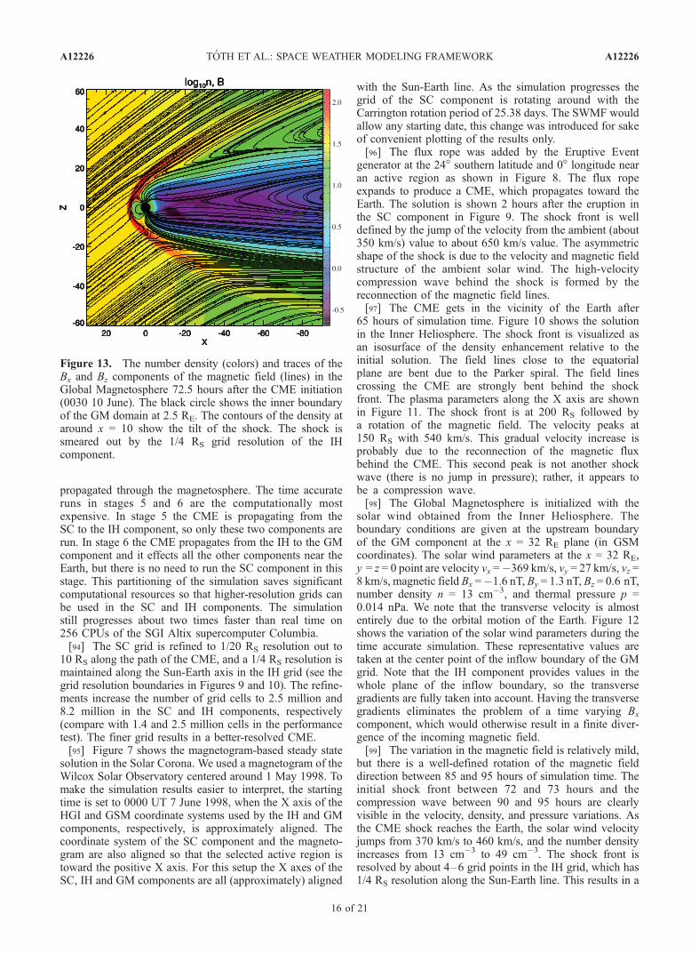
Figure 13. The number density (colors) and traces of theBx and Bz components of the magnetic field (lines) in theGlobal Magnetosphere 72.5 hours after the CME initiation(0030 10 June). The black circle shows the inner boundaryof the GM domain at 2.5 RE. The contours of the density ataround x = 10 show the tilt of the shock. The shock issmeared out by the 1/4 RS grid resolution of the IHcomponent.


16 of 21

A12226

shock width of about 160 RE so the shock front passes inabout 40 min of simulation time.[100] Figure 13 shows the shock front entering the GM

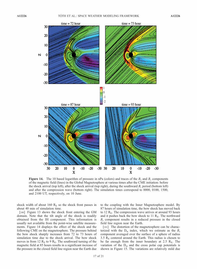
domain. Note that the tilt angle of the shock is readilyobtained from the IH component. This information isusually not available from the point-wise satellite measure-ments. Figure 14 displays the effect of the shock and thefollowing CME on the magnetosphere. The pressure behindthe bow shock sharply increases from 72 to 73 hours ofsimulation time due to the shock arrival. The bow shockmoves in from 12 RE to 9 RE. The southward turning of themagnetic field at 85 hours results in a significant increase ofthe pressure in the closed field line region near the Earth due

to the coupling with the Inner Magnetosphere model. By87 hours of simulation time, the bow shock has moved backto 12 RE. The compression wave arrives at around 93 hoursand it pushes back the bow shock to 11 RE. The northwardBz component results in a reduced pressure in the closedfield line region near the Earth.[101] The distortion of the magnetosphere can be charac-

terized with the Dst index, which we estimate as the Bz

component averaged over the surface of a sphere of radius3.5 RE centered around the Earth. This radius is chosen tobe far enough from the inner boundary at 2.5 RE. Thevariation of the Dst and the cross polar cap potentials isshown in Figure 15. The variations are relatively mild due

Figure 14. The 10 based logarithm of pressure in nPa (colors) and traces of the Bx and Bz componentsof the magnetic field (lines) in the Global Magnetosphere at various times after the CME initiation: beforethe shock arrival (top left), after the shock arrival (top right), during the southward Bz period (bottom left)and after the compression wave (bottom right). The simulation times correspond to 0000, 0100, 1500,and 2100 UT, respectively, on 10 June.


17 of 21

A12226

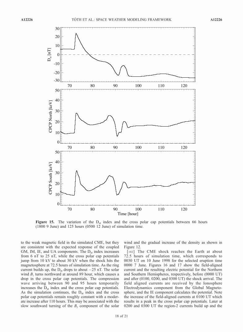
to the weak magnetic field in the simulated CME, but theyare consistent with the expected response of the coupledGM, IM, IE, and UA components. The Dst index increasesfrom 6 nT to 25 nT, while the cross polar cap potentialsjump from 10 kV to about 30 kV when the shock hits themagnetosphere at 72.5 hours of simulation time. As the ringcurrent builds up, the Dst drops to about �25 nT. The solarwind Bz turns northward at around 89 hour, which causes adrop in the cross polar cap potentials. The compressionwave arriving between 90 and 95 hours temporarilyincreases the Dst index and the cross polar cap potentials.As the simulation continues, the Dst index and the crosspolar cap potentials remain roughly constant with a moder-ate increase after 110 hours. This may be associated with theslow southward turning of the Bz component of the solar

wind and the gradual increase of the density as shown inFigure 12.[102] The CME shock reaches the Earth at about

72.5 hours of simulation time, which corresponds to0030 UT on 10 June 1998 for the selected eruption time0000 7 June. Figures 16 and 17 show the field-alignedcurrent and the resulting electric potential for the Northernand Southern Hemispheres, respectively, before (0000 UT)and after (0100, 0200, and 0300 UT) the shock arrival. Thefield aligned currents are received by the IonosphereElectrodynamics component from the Global Magneto-sphere, and the IE component calculates the potential. Notethe increase of the field-aligned currents at 0100 UT whichresults in a peak in the cross polar cap potentials. Later at0200 and 0300 UT the region-2 currents build up and the

Figure 15. The variation of the Dst index and the cross polar cap potentials between 66 hours(1800 9 June) and 125 hours (0500 12 June) of simulation time.


18 of 21

A12226

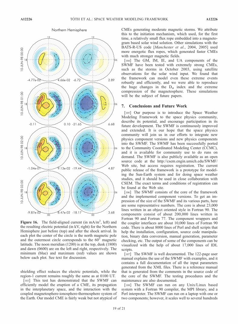
shielding effect reduces the electric potentials, while theregion-1 current remains roughly the same as at 0100 UT.[103] This test has demonstrated that the SWMF can

efficiently model the eruption of a CME, its propagationin the interplanetary space, and the interaction with thecoupled magnetosphere-ionosphere-thermosphere system ofthe Earth. Our model CME is fairly weak but not atypical of

CMEs generating moderate magnetic storms. We attributethis to the initiation mechanism, which used, for the firsttime, a relatively small flux rope embedded into a magneto-gram based solar wind solution. Other simulations with theBATS-R-US code [Manchester et al., 2004, 2005] usedmore energetic flux ropes, which generated faster CMEswith much stronger magnetic fields.[104] The GM, IM, IE, and UA components of the

SWMF have been tested with extremely strong CMEs,such as the storms in October 2003, using satelliteobservations for the solar wind input. We found thatthe framework can model even these extreme eventsrobustly and efficiently, and we were able to reproducethe huge changes in the Dst index and the extremecompression of the magnetosphere. These simulationswill be the subject of future papers.

7. Conclusions and Future Work

[105] Our purpose is to introduce the Space WeatherModeling Framework to the space physics community,describe its potential, and encourage participation in itsfuture development. The SWMF is continuously improvedand extended. It is our hope that the space physicscommunity will join us in our efforts to integrate newphysics component versions and new physics componentsinto the SWMF. The SWMF has been successfully portedto the Community Coordinated Modeling Center (CCMC),and it is available for community use to do runs ondemand. The SWMF is also publicly available as an opensource code at the http://csem.engin.umich.edu/SWMF/Web site, but access requires registration. The currentpublic release of the framework is a prototype for model-ing the Sun-Earth system and for doing space weatherstudies, and it should be used in close collaboration withCSEM. The exact terms and conditions of registration canbe found at the Web site.[106] The SWMF consists of the core of the framework

and the implemented component versions. To get an im-pression of the size of the SWMF and its various parts, hereare some representative numbers. The core is about 23,000lines written in an object oriented style in Fortran 90. Thecomponents consist of about 200,000 lines written inFortran 90 and Fortran 77. The component wrappers andthe coupler interfaces are about 10,000 lines of Fortran 90code. There is about 8000 lines of Perl and shell scripts thathelp the installation, configuration, source code manipula-tion, binary data conversion, manual generation, parameterchecking, etc. The output of some of the components can bevisualized with the help of about 17,000 lines of IDLscripts.[107] The SWMF is well documented. The 122-page user

manual explains the use of the SWMF with examples, and itcontains a full documentation of all the input parametersgenerated from the XML files. There is a reference manualthat is generated from the comments in the source code ofthe core of the SWMF. The testing procedures and themaintenance are also documented.[108] The SWMF can run on any Unix/Linux based

system with a Fortran 90 compiler, the MPI library, and aPerl interpreter. The SWMF can run on a laptop with one ortwo components; however, it scales well to several hundreds

Figure 16. The field-aligned current (in mA/m2, left) andthe resulting electric potential (in kV, right) for the NorthernHemisphere just before (top) and after the shock arrival. Ineach plot the center of the circle is the north magnetic poleand the outermost circle corresponds to the 60� magneticlatitude. The noon meridian (1200) is at the top, dusk (1800)and dawn (0600) are on the left and right, respectively. Theminimum (blue) and maximum (red) values are shownbelow each plot. See text for discussion.


19 of 21

A12226

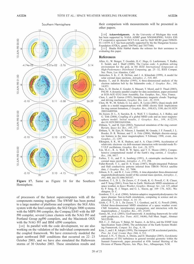
of processors of the fastest supercomputers with all thecomponents running together. The SWMF has been portedto a large number of platforms and compilers: the SGI Altixsystem with the Intel compiler, the SGI Origin 3000 systemswith the MIPS f90 compiler, the Compaq ES45 with the HPf90 compiler, several Linux clusters with the NAG f95 andPortland Group pgf90 compilers, and the Macintosh OSXwith the NAG f95 and IBM xlf90 compilers.[109] In parallel with the code development, we are also

working on the validation of the individual components andthe coupled framework. We have extensively modeled thequiet northward IMF conditions that occurred on 22–23October 2003, and we have also simulated the Halloweenstorms of 30 October 2003. These simulation results and

their comparison with measurements will be presented inother papers.

[110] Acknowledgments. At the University of Michigan this workhas been supported by NASA AISRP grant NNG04GP89G, NASA ESSCT cooperative agreement NCC5-614, and by DoD MURI grant F49620-01-1-0359. G.T. has been partially supported by the the Hungarian ScienceFoundation (OTKA, grants T047042 and T037548).[111] Shadia Rifai Habbal thanks the referees for their assistance in

evaluating this paper.

ReferencesAllen, G., W. Benger, T. Goodale, H.-C. Hege, G. Lanfermann, T. Radke,E. Seidel, and J. Shalf (2000), The Cactus code: A problem solvingenvironment for the grid, in 9th IEEE International Symposium onHigh-Performance Distributed Computing, pp. 25–32, IEEE Comput.Soc. Press, Los Alamitos, Calif.

Antiochos, S. K., C. R. DeVore, and J. A. Klimchuk (1999), A model forsolar coronal mass ejections, Astrophys. J., 510, 485.

Beutier, T., and D. Boscher (1995), A three-dimensional analysis of theelectron radiation belt by the Salammbo code, J. Geophys. Res., 100,14,853.

Buis, S., D. Declat, E. Gondet, S. Massart, T. Morel, and O. Thual (2003),PALM: A dynamic parallel coupler for data assimilation, paper presentedat EGS-AGU-EUG Joint Assembly, Eur. Geophys. Soc., Nice, France.

Chen, J., and D. Garren (1993), Interplanetary magnetic clouds: Topologyand driving mechanism, Geophys. Res. Lett., 20, 2319.

Chen, M. W., M. Schulz, G. Lu, and L. R. Lyons (2003), Quasi-steady driftpaths in a model magnetosphere with AMIE electric field: Implicationsfor ring current formation, J. Geophys. Res., 108(A5), 1180, doi:10.1029/2002JA009584.

De Zeeuw, D. L., S. Sazykin, R. A. Wolf, T. I. Gombosi, A. J. Ridley, andG. Toth (2004), Coupling of a global MHD code and an inner magneto-sphere model: Initial results, J. Geophys. Res., 109, A12219,doi:10.1029/2003JA010366.

Ebihara, Y., and M. Ejiri (2002), Numerical simulation of the ring current:Review, Space Sci. Rev., 105, 377.

Ebihara, Y., M. Ejiri, H. Nilsson, I. Sandahl, M. Grande, J. F. Fennell, J. L.Roeder, D. R. Weimer, and T. A. Fritz (2004), Multiple discrete-energyion features in the inner magnetosphere: 9 February 1998, event, Ann.Geophys., 22, 1297.

Elkington, S. R., M. K. Hudson, and A. A. Chan (1999), Acceleration ofrelativistic electrons via drift-resonant interaction with toroidal-mode Pc-5 ULF oscillations, Geophys. Res. Lett., 26, 3273.

Fok, M.-C., R. A. Wolf, R. W. Spiro, and T. E. Moore (2001), Compre-hensive computational model of the Earth’s ring current, J. Geophys.Res., 106, 8417.

Forbes, T. G., and P. A. Isenberg (1991), A catastrophe mechanism forcoronal mass ejections, Astrophys. J., 373, 294.

Fuller-Rowell, T. J., and D. S. Evans (1987), Height-integrated Pedersenand Hall conductivity patterns inferred from TIROS–NOAA satellitedata, J. Geophys. Res., 92, 7606.

Gibson, S. E., and B. C. Low (1998), A time-dependent three-dimensionalmagnetohydrodynamic model of the coronal mass ejection, Astrophys. J.,493, 460, doi:10.1086/305107.

Gombosi, T. I., D. L. De Zeeuw, C. P. Groth, K. G. Powell, C. R. Clauer,and P. Song (2001), From Sun to Earth: Multiscale MHD simulations ofspace weather, in Space Weather, Geophys. Monogr. Ser., vol. 125, editedby P. Song, H. J. Singer, and G. L. Siscoe, pp. 169–176, AGU, Wa-shington, D. C.

Gombosi, T. I., et al. (2004), Solution-adaptive magnetohydrodynamics forspace plasmas: Sun-to-Earth simulations, computing in science and en-gineering, Frontiers Simul., 6, 14–35.

Groth, C. P. T., D. L. De Zeeuw, T. I. Gombosi, and K. G. Powell (2000),Global three-dimensional MHD simulation of a space weather event:CME formation, interplanetary propagation, and interaction with themagnetosphere, J. Geophys. Res., 105, 25,053.

Gurnis, M., et al. (2003), GeoFramework: A modeling framework for solidearth geophysics, Eos. Trans. AGU, 84(46), Fall Meet. Suppl., AbstractNG12D-06.

Hill, C., C. DeLuca, V. Balaji, M. Suarez, A. da Silva, and the ESMF JointSpecification Team (2004), The architecture of the Earth System Model-ing Framework, Comput. Sci. Eng., 6, 18.

Kota, J., and J. R. Jokipii (1999), The transport of CIR accelerated particles,Proc. Int. Conf. Cosmic Rays 26th, 6, 512.

Leboeuf, J.-N., V. Decyk, A. Dimits, and D. Shumaker (2003), Gyrokineticcalculations of ITG turbulence in general toroidal geometry within theSummit Framework, paper presented at 45th Annual Meeting of theDivision of Plasma Physics, Am. Phys. Soc., Albuquerque, N.M.

Figure 17. Same as Figure 16 for the SouthernHemisphere.


20 of 21

A12226

Liemohn, M. W., A. J. Ridley, D. L. Gallagher, D. M. Ober, and J. U.Kozyra (2004), Dependence of plasmaspheric morphology on theelectric field description during the recovery phase of the April 17,2002 magnetic storm, J. Geophys. Res., 109, A03209, doi:10.1029/2003JA010304.

Low, B. C. (2001), Coronal mass ejections, magnetic flux ropes, and solarmagnetism, J. Geophys. Res., 106, 25,141.

Luhmann, J. G., S. C. Solomon, J. A. Linker, J. G. Lyon, Z. Mikic,D. Odstrcil, W. Wang, and M. Wiltberger (2004), Coupled modelsimulation of a Sun-to-Earth space weather event, J. Atmos. Sol.Terr. Phys., 66, 1243.

Manchester, W. B., IV (2003), Buoyant disruption of magnetic arcades withself-induced shearing, J. Geophys. Res., 108(A4), 1162, doi:10.1029/2002JA009252.

Manchester, W. B., IV, T. I. Gombosi, I. I. Roussev, A. J. Ridley, D. L. DeZeeuw, I. V. Sokolov, K. G. Powell, and G. Toth (2004), Modeling aspace weather event from the Sun to the Earth: CME generation andinterplanetary propagation, J. Geophys. Res. , 109 , A02107,doi:10.1029/2003JA010150.

Manchester, W. B., IV, A. J. Ridley, T. I. Gombosi, and D. L. De Zeeuw(2005), Modeling the Sun-Earth propagation of a very fast CME, Adv.Space Res., in press.

Moen, J., and A. Brekke (1993), The solar flux influence of quiet-timeconductances in the auroral ionosphere, Geophys. Res. Lett., 20, 971.

Powell, K. G., P. L. Roe, T. J. Linde, T. I. Gombosi, and D. L. De Zeeuw(1999), A solution-adaptive upwind scheme for ideal magnetohydrody-namics, J. Comput. Phys., 154(2), 284, doi:10.1006/jcph.1999.6299.

Reynders, J. (1996), POOMA: A framework for scientific simulationson parallel architectures, in Parallel Programming Using C++, editedby G. F. Wilson and P. Lu, pp. 553–594, MIT Press, Cambridge, Mass.

Richmond, A. D., and Y. Kamide (1988), Mapping Electrodynamic featuresof the high-latitude ionosphere from localized observations: Technique,J. Geophys. Res., 93, 5741.

Richmond, A. D., E. C. Ridley, and R. G. Roble (1992), A thermosphere/ionosphere general circulation model with coupled electrodynamics,J. Geophys. Res., 96, 1071.

Ridley, A. J., and M. W. Liemohn (2002), A model-derived stormtimeasymmetric ring current driven electric field description, J. Geophys.Res., 107(A8), 1151, doi:10.1029/2001JA000051.

Ridley, A. J., D. L. De Zeeuw, T. I. Gombosi, and K. G. Powell (2001),Using steady-state MHD results to predict the global state of the magne-tosphere-ionosphere system, J. Geophys. Res., 106, 30,067.

Ridley, A. J., T. I. Gombosi, D. L. De Zeeuw, C. R. Clauer, and A. D.Richmond (2003), Ionospheric control of the magnetospheric configura-tion: Neutral winds, J. Geophys. Res., 108(A8), 1328, doi:10.1029/2002JA009464.

Ridley, A. J., T. I. Gombosi, and D. L. De Zeeuw (2004), Ionosphericcontrol of the magnetospheric configuration: Conductance, Ann. Geo-phys., 22, 567.

Robinson, R. M., R. R. Vondrak, K. Miller, T. Dabbs, and D. A. Hardy(1987), On calculating ionospheric conductances from the flux andenergy of precipitating electrons, J. Geophys. Res., 92, 2565.

Roussev, I. I., T. G. Forbes, T. I. Gombosi, I. V. Sokolov, D. L. DeZeeuw, and J. Birn (2003a), A three-dimensional flux rope model forcoronal mass ejections based on a loss of equilibrium, Astrophys. J.,588, L45.

Roussev, I. I., T. I. Gombosi, I. V. Sokolov, M. Velli, W. Manchester, D. L.De Zeeuw, P. Liewer, G. Toth, and J. Luhmann (2003b), A three-dimen-sional model of the solar wind incorporating solar magnetogram observa-tions, Astrophys. J., 595, L57.

Roussev, I. I., I. V. Sokolov, T. G. Forbes, T. I. Gombosi, M. A. Lee, andJ. I. Sakai (2004), A numerical model of a coronal mass ejection: Shockdevelopment with implications for the acceleration of GeV protons,Astrophys. J., 605, L73.

Shprits, Y. Y., and R. M. Thorne (2004), Time dependent radial diffusionmodeling of relativistic electrons with realistic loss rates, Geophys. Res.Lett., 31, L08805, doi:10.1029/2004GL019591.

Sokolov, I. V., I. I. Roussev, T. I. Gombosi, M. A. Lee, J. Kota, T. G.Forbes, W. B. Manchester, and J. I. Sakai (2004), A new fieldline advection model for solar particle acceleration, Astrophys.J., 616:L171, L174.

Toffoletto, F., S. Sazykin, R. Spiro, and R. Wolf (2003), Inner magneto-spheric modeling with the Rice Convection Model, Space Sci. Rev., 107,175.

Usmanov, A. V., M. L. Goldstein, B. P. Besser, and J. M. Fritzer (2000), Aglobal MHD solar wind model with WKB Alfvn waves: Comparisonwith Ulysses data, J. Geophys. Res., 105, 12,675.

Weimer, D. R. (1996), A flexible, IMF dependent model of high-latitudeelectric potential having ‘‘space weather’’ applications, Geophys. Res.Lett., 23, 2549.

Wolf, R. A., M. Harel, R. W. Spiro, G.-H. Voigt, P. H. Reiff, and C. K. Chen(1982), Computer simulation of inner magnetospheric dynamics for themagnetic storm of July 29, 1977, J. Geophys. Res., 87, 5949.

Wu, S. T., W. P. Guo, D. J. Michels, and L. F. Bulgara (1999),MHD description of the dynamical relationships between a flux rope,streamer, coronal mass ejection, and magnetic cloud: An analysis ofthe January 1997 Sun-Earth connection event, J. Geophys. Res., 104,14,789.

Wu, S. T., W. P. Guo, S. P. Plunkett, B. Schmieder, and G. M. Simnett(2000), Coronal mass ejections (CMEs) initiation: Models and observa-tions, J. Atmos. Sol. Terr. Phys., 62, 1489.

��A. Chan, S. Sazykin, R. A. Wolf, and B. Yu, Rice University, MS-108,

6100 South Main Street, Houston, TX 77005-1892, USA.D. R. Chesney, C. R. Clauer, D. L. De Zeeuw, T. I. Gombosi, K. C.

Hansen, K. J. Kane, W. B. Manchester, R. C. Oehmke, K. G. Powell, A. J.Ridley, I. I. Roussev, G. Toth, I. V. Sokolov, Q. F. Stout, and O. Volberg,Center for Space Environment Modeling, University of Michigan, AnnArbor, MI 48109-2143, USA. ([email protected])J. Kota, University of Arizona, 1629 E. University Blvd., Tucson, AZ

85721, USA.


21 of 21

A12226

Documents

Space Weather Modeling Framework: A new tool for the space ...web.eecs.umich.edu/~qstout/pap/JGeoRes05.pdf · Space Weather Modeling Framework: A new tool for the space science community