Embed Size (px)
Citation preview

. . .
. . . . .
Introduction. . . . . . .. . . . . .. . . . . . . .
Sparrow Evaluation
SPARROWSPARse appROximation Weighted regression
Pardis Noorzad
Department of Computer Engineering and ITAmirkabir University of Technology
Universite de Montreal – March 12, 2012
SPARROW 1/47

. . .
. . . . .
Introduction. . . . . . .. . . . . .. . . . . . . .
Sparrow Evaluation
Outline
IntroductionMotivationLocal Methods
SparrowSPARROW is a Local MethodDefining the Effective WeightsDefining the Observation Weights
Evaluation
SPARROW 2/47

. . .
. . . . .
Introduction. . . . . . .. . . . . .. . . . . . . .
Sparrow Evaluation
Motivation
Problem setting
I Given D := (xi, yi) : i = 1, . . . , NI yi ∈ R is the output
I at the input xi := [xi1, . . . , xiM ]T ∈ RM
I our task is to estimate the regression function
f : RM 7→ R
such thatyi = f(xi) + ϵi
the ϵi’s are independent with zero mean.
SPARROW 5/47
. . .
. . . . .
Introduction. . . . . . .. . . . . .. . . . . . . .
Sparrow Evaluation
Motivation
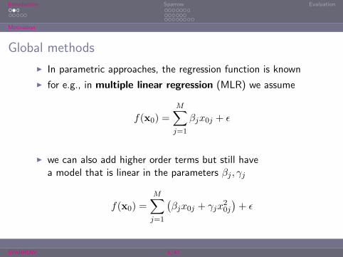
Global methods
I In parametric approaches, the regression function is known
I for e.g., in multiple linear regression (MLR) we assume
f(x0) =
M∑j=1
βjx0j + ϵ
I we can also add higher order terms but still havea model that is linear in the parameters βj , γj
f(x0) =
M∑j=1
(βjx0j + γjx
20j
)+ ϵ
SPARROW 6/47
. . .
. . . . .
Introduction. . . . . . .. . . . . .. . . . . . . .
Sparrow Evaluation
Motivation
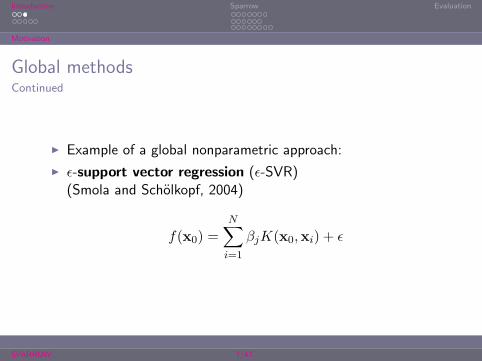
Global methodsContinued
I Example of a global nonparametric approach:
I ϵ-support vector regression (ϵ-SVR)(Smola and Scholkopf, 2004)
f(x0) =
N∑i=1
βjK(x0,xi) + ϵ
SPARROW 7/47
. . .
. . . . .
Introduction. . . . . . .. . . . . .. . . . . . . .
Sparrow Evaluation
Local Methods
Local methods
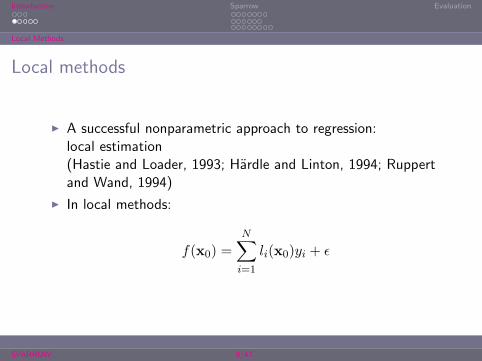
I A successful nonparametric approach to regression:local estimation(Hastie and Loader, 1993; Hardle and Linton, 1994; Ruppertand Wand, 1994)
I In local methods:
f(x0) =N∑i=1
li(x0)yi + ϵ
SPARROW 9/47
. . .
. . . . .
Introduction. . . . . . .. . . . . .. . . . . . . .
Sparrow Evaluation
Local Methods
Local methodsContinued
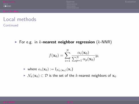
I For e.g. in k-nearest neighbor regression (k-NNR)
f(x0) =
N∑i=1
αi(x0)∑Np=1 αp(x0)
yi
I where αi(x0) := INk(x0)(xi)
I Nk(x0) ⊂ D is the set of the k-nearest neighbors of x0
SPARROW 10/47
. . .
. . . . .
Introduction. . . . . . .. . . . . .. . . . . . . .
Sparrow Evaluation
Local Methods
Local methodsContinued
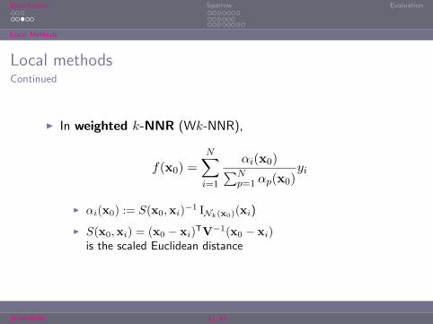
I In weighted k-NNR (Wk-NNR),
f(x0) =
N∑i=1
αi(x0)∑Np=1 αp(x0)
yi
I αi(x0) := S(x0,xi)−1 INk(x0)(xi)
I S(x0,xi) = (x0 − xi)TV−1(x0 − xi)
is the scaled Euclidean distance
SPARROW 11/47
. . .
. . . . .
Introduction. . . . . . .. . . . . .. . . . . . . .
Sparrow Evaluation
Local Methods
Local methodsContinued
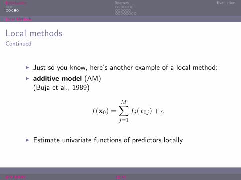
I Just so you know, here’s another example of a local method:
I additive model (AM)(Buja et al., 1989)
f(x0) =M∑j=1
fj(x0j) + ϵ
I Estimate univariate functions of predictors locally
SPARROW 12/47
. . .
. . . . .
Introduction. . . . . . .. . . . . .. . . . . . . .
Sparrow Evaluation
Local Methods
Local methodsContinued
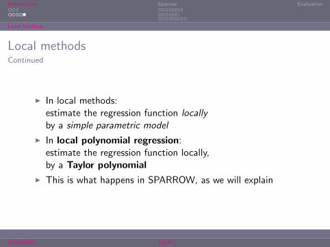
I In local methods:estimate the regression function locallyby a simple parametric model
I In local polynomial regression:estimate the regression function locally,by a Taylor polynomial
I This is what happens in SPARROW, as we will explain
SPARROW 13/47

. . .
. . . . .
Introduction. . . . . . .. . . . . .. . . . . . . .
Sparrow Evaluation
SPARROW is a Local Method
Sparrow
SPARROW 16/47

. . .
. . . . .
Introduction. . . . . . .. . . . . .. . . . . . . .
Sparrow Evaluation
SPARROW is a Local Method
I meant this sparrow
SPARROW 17/47

. . .
. . . . .
Introduction. . . . . . .. . . . . .. . . . . . . .
Sparrow Evaluation
SPARROW is a Local Method
SPARROW is a local method
I Before we get into the details,
I see a few examples showing benefits of local methods
I then we’ll talk about SPARROW
SPARROW 18/47
−1 −0.8 −0.6 −0.4 −0.2 0 0.2 0.4 0.6 0.8 1−0.6
−0.4
−0.2
0
0.2
0.4
0.6
0.8
1
Goal functionDataset
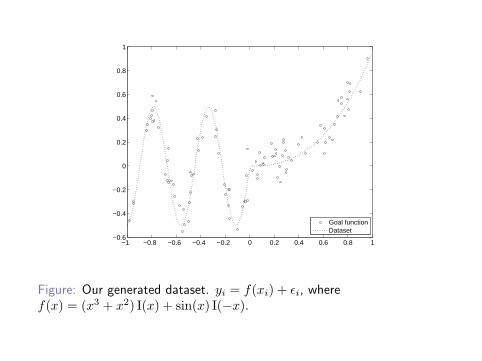
Figure: Our generated dataset. yi = f(xi) + ϵi, wheref(x) = (x3 + x2) I(x) + sin(x) I(−x).
−1 −0.8 −0.6 −0.4 −0.2 0 0.2 0.4 0.6 0.8 1−0.6
−0.4
−0.2
0
0.2
0.4
0.6
0.8
1
DatasetGoal functionMLR:1stMLR:2ndMLR:3rd
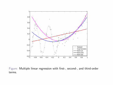
Figure: Multiple linear regression with first-, second-, and third-orderterms.
−1 −0.8 −0.6 −0.4 −0.2 0 0.2 0.4 0.6 0.8 1−0.6
−0.4
−0.2
0
0.2
0.4
0.6
0.8
1
DatasetGoal functionε−SVR
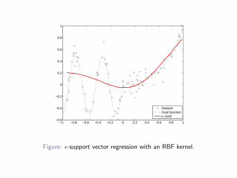
Figure: ϵ-support vector regression with an RBF kernel.
−1 −0.8 −0.6 −0.4 −0.2 0 0.2 0.4 0.6 0.8 1−0.6
−0.4
−0.2
0
0.2
0.4
0.6
0.8
1
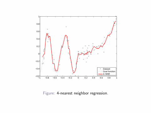
DatasetGoal function4−NNR
Figure: 4-nearest neighbor regression.
. . .
. . . . .
Introduction. . . . . . .. . . . . .. . . . . . . .
Sparrow Evaluation
Defining the Effective Weights
Effective weights in SPARROW
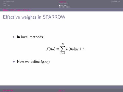
I In local methods:
f(x0) =
N∑i=1
li(x0)yi + ϵ
I Now we define li(x0)
SPARROW 24/47
. . .
. . . . .
Introduction. . . . . . .. . . . . .. . . . . . . .
Sparrow Evaluation
Defining the Effective Weights
Local estimation by a Taylor polynomial
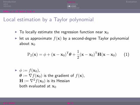
I To locally estimate the regression function near x0
I let us approximate f(x) by a second-degree Taylor polynomialabout x0
P2(x) = ϕ+ (x− x0)Tθ +
1
2(x− x0)
TH(x− x0) (1)
I ϕ := f(x0),θ := ∇f(x0) is the gradient of f(x),H := ∇2f(x0) is its Hessianboth evaluated at x0
SPARROW 25/47
. . .
. . . . .
Introduction. . . . . . .. . . . . .. . . . . . . .
Sparrow Evaluation
Defining the Effective Weights
Local estimation by a Taylor polynomialContinued
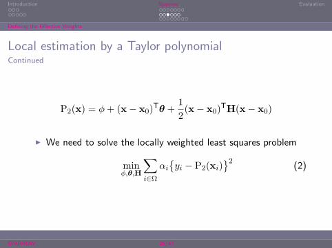
P2(x) = ϕ+ (x− x0)Tθ +
1
2(x− x0)
TH(x− x0)
I We need to solve the locally weighted least squares problem
minϕ,θ,H
∑i∈Ω
αi
yi − P2(xi)
2(2)
SPARROW 26/47
. . .
. . . . .
Introduction. . . . . . .. . . . . .. . . . . . . .
Sparrow Evaluation
Defining the Effective Weights
Local estimation by a Taylor polynomialContinued
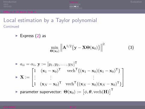
I Express (2) as
minΘ(x0)
∥∥∥A1/2y −XΘ(x0)
∥∥∥2 (3)
I aii = αi, y := [y1, y2, . . . , yN ]T
I X :=
1 (x1 − x0)T vechT(x1 − x0)(x1 − x0)
T...
......
1 (xN − x0)T vechT(xN − x0)(xN − x0)
T
I parameter supervector: Θ(x0) :=
[ϕ,θ, vech(H)
]TSPARROW 27/47
. . .
. . . . .
Introduction. . . . . . .. . . . . .. . . . . . . .
Sparrow Evaluation
Defining the Effective Weights
Local estimation by a Taylor polynomialContinued
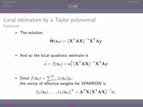
I The solution:
Θ(x0) =(XTAX
)−1XTAy
I And so the local quadratic estimate is
ϕ = f(x0) = eT1(XTAX
)−1XTAy
I Since f(x0) =∑N
i=1 li(x0)yi,the vector of effective weights for SPARROW is
[l1(x0), . . . , lN (x0)]T = ATX
(XTAX
)−1e1
SPARROW 28/47
. . .
. . . . .
Introduction. . . . . . .. . . . . .. . . . . . . .
Sparrow Evaluation
Defining the Effective Weights
Local estimation by a Taylor polynomialContinued
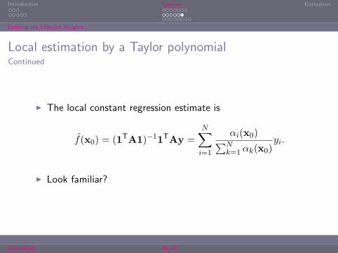
I The local constant regression estimate is
f(x0) = (1TA1)−11TAy =
N∑i=1
αi(x0)∑Nk=1 αk(x0)
yi.
I Look familiar?
SPARROW 29/47
. . .
. . . . .
Introduction. . . . . . .. . . . . .. . . . . . . .
Sparrow Evaluation
Defining the Observation Weights
Observation weights in SPARROW
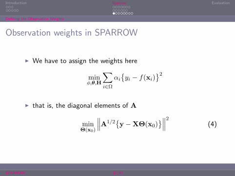
I We have to assign the weights here
minϕ,θ,H
∑i∈Ω
αi
yi − f(xi)
2I that is, the diagonal elements of A
minΘ(x0)
∥∥∥A1/2y −XΘ(x0)
∥∥∥2 (4)
SPARROW 31/47
. . .
. . . . .
Introduction. . . . . . .. . . . . .. . . . . . . .
Sparrow Evaluation
Defining the Observation Weights
Observation weights in SPARROWContinued
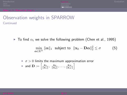
I To find αi we solve the following problem (Chen et al., 1995)
minα∈RN
∥α∥1 subject to ∥x0 −Dα∥22 ≤ σ (5)
I σ > 0 limits the maximum approximation error
I and D :=[
x1
∥x1∥ ,x2
∥x2∥ , . . . ,xN
∥xN∥
]
SPARROW 32/47

. . .
. . . . .
Introduction. . . . . . .. . . . . .. . . . . . . .
Sparrow Evaluation
Defining the Observation Weights
Power family of penaltiesℓp norms raised to the pth power
∥x∥pp =
(∑i
|xi|p)
(6)
I For 1 ≤ p < ∞, (6) is convex.
I 0 < p ≤ 1, is the range of p useful for measuring sparsity.
SPARROW 33/47
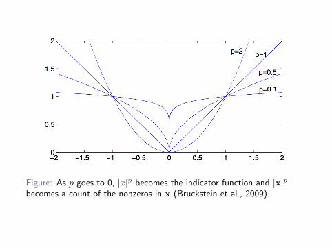
Figure: As p goes to 0, |x|p becomes the indicator function and |x|pbecomes a count of the nonzeros in x (Bruckstein et al., 2009).

. . .
. . . . .
Introduction. . . . . . .. . . . . .. . . . . . . .
Sparrow Evaluation
Defining the Observation Weights
Representation by sparse approximationContinued
I To motivate this idea let’s look atI feature learning with sparse coding, and
I sparse representation classification (SRC)I an example of exemplar-based sparse approximation
SPARROW 35/47
. . .
. . . . .
Introduction. . . . . . .. . . . . .. . . . . . . .
Sparrow Evaluation
Defining the Observation Weights
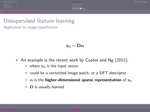
Unsupervised feature learningApplication to image classification
x0 = Dα
I An example is the recent work by Coates and Ng (2011).I where x0 is the input vector
I could be a vectorized image patch, or a SIFT descriptor
I α is the higher-dimensional sparse representation of x0
I D is usually learned
SPARROW 36/47
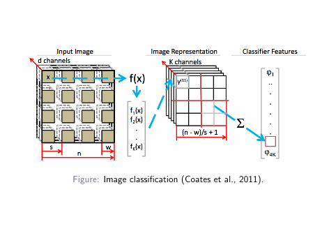
Figure: Image classification (Coates et al., 2011).

. . .
. . . . .
Introduction. . . . . . .. . . . . .. . . . . . . .
Sparrow Evaluation
Defining the Observation Weights
Multiclass classification(Wright et al., 2009)
I D :=(xi, yi) : xi ∈ Rm, yi ∈ 1, . . . , c, i ∈ 1, . . . , N
I Given a test sample x0
1. Solve minα∈RN ∥α∥1 subject to ∥x0 −Dα∥22 ≤ σ2. Define αy : y ∈ 1, . . . , c where [αy]i = αi if xi belongs to
class y, o.w. 03. Construct X (α) :=
xy(α) = Dαy, y ∈ 1, . . . , c
4. Predict y := argminy∈1,...,c ∥x0 − xy(α)∥22
SPARROW 38/47
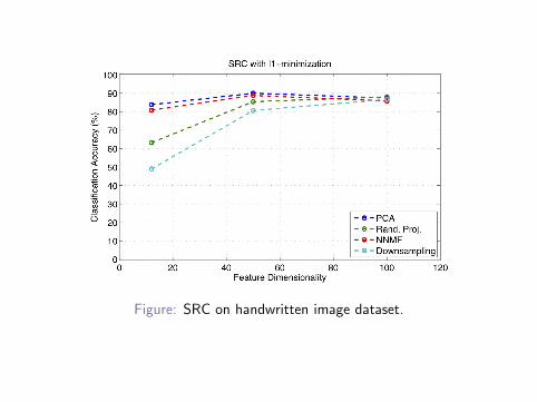
Figure: SRC on handwritten image dataset.
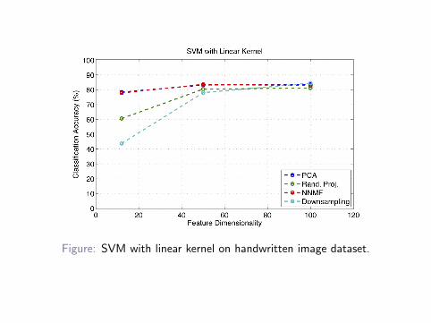
Figure: SVM with linear kernel on handwritten image dataset.
. . .
. . . . .
Introduction. . . . . . .. . . . . .. . . . . . . .
Sparrow Evaluation
Back to SPARROW with evaluation on the MPG dataset
I Auto MPG Data Set
I from the UCI Machine Learning Repository (Frank andAsuncion, 2010)
I “The data concerns city-cycle fuel consumption in miles pergallon, to be predicted in terms of 3 multivalued discrete and4 continuous attributes.”
I number of instances: 392
I number of attributes: 7 (cylinders, displacement, horsepower,weight, acceleration, model year, origin)
SPARROW 42/47
4
6
8
10
12
14
16
18
1 2 3 4 5 6
MS
E
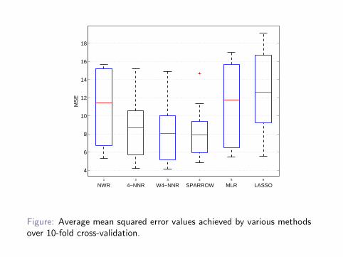
NWR 4−NNR W4−NNR SPARROW MLR LASSO
Figure: Average mean squared error values achieved by various methodsover 10-fold cross-validation.

. . .
. . . . .
Introduction. . . . . . .. . . . . .. . . . . . . .
Sparrow Evaluation
Looking ahead
I What is causing the success of SPARROW and SRC?
I How important is the bandwidth? What about in SRC?
SPARROW 44/47

References
References I
Alfred M. Bruckstein, David L. Donoho, and Michael Elad. From sparsesolutions of systems of equations to sparse modeling of signals and images.SIAM Review, 51(1):34–81, 2009.
Andreas Buja, Trevor Hastie, and Robert Tibshirani. Linear smoothers andadditive models. The Annals of Statistics, 17(2):435–555, 1989.
Scott S. Chen, David L. Donoho, and Michael A. Saunders. Atomicdecomposition by basis pursuit. Technical Report 479, Department ofStatistics, Stanford University, May 1995.
Adam Coates and Andrew Ng. The importance of encoding versus trainingwith sparse coding and vector quantization. In International Conference onMachine Learning (ICML), pages 921–928, 2011.
Adam Coates, Honglak Lee, and Andrew Y. Ng. Self-taught learning: Transferlearning from unlabeled data. In International Conference on AI andStatistics, 2011.
SPARROW 45/47
References
References II
A. Frank and A. Asuncion. UCI machine learning repository, 2010. URLhttp://archive.ics.uci.edu/ml.
Wolfgang Hardle and Oliver Linton. Applied nonparametric methods. TechnicalReport 1069, Yale University, 1994.
T. J. Hastie and C. Loader. Local regression: Automatic kernel carpentry.Statistical Science, 8(2):120–129, 1993.
D. Ruppert and M. P. Wand. Multivariate locally weighted least squaresregression. The Annals of Statistics, 22:1346–1370, 1994.
Alex J. Smola and Bernhard Scholkopf. A tutorial on support vector regression.Statistics and Computing, 14:199–222, August 2004.
John Wright, Allen Y. Yang, Arvind Ganesh, S. Shankar Sastry, and Yi Ma.Robust face recognition via sparse representation. IEEE Transactions onPattern Analysis and Machine Intelligence, 31:210–227, 2009.
SPARROW 46/47

References
Acknowledgements
I This is ongoing work carried out under the supervision ofProf. Bob L. Sturm of Aalborg University Copenhagen.
I Thanks to Isaac Nickaein and Sheida Bijanifor helping out with the slides.
SPARROW 47/47