KURT KONOLIGE: SPARSE SPARSE BUNDLE ADJUSTMENT 1

Sparse Sparse Bundle Adjustment

Kurt Konoligehttp://www.willowgarage.com/~konolige

Willow Garage68 Willow RoadMenlo Park, USA

Abstract

Sparse Bundle Adjustment (SBA) is a method for simultaneously optimizing a set ofcamera poses and visible points. It exploits the sparse primary structure of the problem,where connections exist just between points and cameras. In this paper, we implementan efficient version of SBA for systems where the secondary structure (relations amongcameras) is also sparse. The method, which we call Sparse SBA (sSBA), integratesan efficient method for setting up the linear subproblem with recent advances in directsparse Cholesky solvers. sSBA outperforms the current SBA standard implementationon datasets with sparse secondary structure by at least an order of magnitude, while alsobeing more efficient on dense datasets.

1 IntroductionSparse Bundle Adjustment (SBA) is the standard method for optimizing a structure-from-motion problem in computer vision. With the success of Photosynth and similar systemsfor stitching together large collections of images [16], attention has turned to the problem ofmaking SBA more efficient. There are two different types of large-scale systems:

• Photosynth-type systems focus on reconstruction from a large number of images con-centrated in a small area; we call these object-centered.

• Visual mapping systems [1, 3, 9] cover a more extended area with fewer images, andreal-time performance is often important (see Figure 1).

These types are at two ends of a spectrum: object-centered systems produce dense relationsbetween cameras, while visual mapping systems are much sparser, with cameras in a localneighborhood sharing common points (Guilbert et al. call these “sparse systems” [8]). Inthis paper, we are interested in fast SBA methods for the latter case, where it is possible toexploit the sparse secondary structure (camera to camera relations) of the problem.

Nonlinear optimization in SBA typically proceeds by iteration: form a linear subproblemaround the current solution, solve it, and repeat until convergence. For large problems, thecomputational bottleneck is usually the solution of the linear subproblem, which can growas the cube of the number of cameras. The fill-in of the linear problem is directly tiedto the camera-point structure of the problem: if each camera only sees features in a smallneighborhood of other cameras, the number of non-zero elements grows only linearly ornearly linearly with the number of cameras.

c© 2010. The copyright of this document resides with its authors.It may be distributed unchanged freely in print or electronic forms.

BMVC 2010 doi:10.5244/C.24.102

2 KURT KONOLIGE: SPARSE SPARSE BUNDLE ADJUSTMENT

Figure 1: An overhead view showing of the New College mapping dataset [15], with 2.2kviews (cyan) and 290k points (red). Grid lines are at 10 m. At the end, sSBA computes eachiteration in 6 seconds.

In this paper we present an engineering approach to efficiently solving SBA problemswith sparse linear subproblems. Our approach is to exploit recent fast direct Cholesky de-composition methods to solve the linear subproblem. These methods use a compressed rep-resentation of large sparse matrices, and we present a method for efficiently handling theblock data structures of SBA to take advantage of this representation. The end result is a sys-tem, which we call Sparse SBA or sSBA, that outperforms the current reference system forSBA from Lourakis and Argyros [11] by an order of magnitude on sparse seconary-structureproblems, and uses far less space on large problems. For example, Figure 1 shows a recon-struction of a New College dataset [15] that contains 2200 views and 290k points, and issolved in about 6 seconds per iteration at the end. Interestingly, sSBA also outperforms [11]on problems with dense secondary structure, where the setup computation often dominates,although by a lesser margin.

2 Related Work

The standard reference for SBA is the monograph of Triggs et al. [17]. This work exploresmany of the mathematical and computational aspects of SBA, including various methodsfor solving the nonlinear optimization problem at the heart of SBA. In this paper, we useLevenberg-Marquardt [14], which is a standard algorithm for solving unconstrained nonlin-ear optimization. Alternative solvers for SBA include preconditioned conjugate gradient [2]or Powell’s dog-leg solver [12].

The LM implementation of SBA repeatedly solves a large linear subproblem whose LHSmatrix is positive definite. Recent work in direct sparse Cholesky solvers [4] has yieldedalgorithms that are very efficient for large problems, and we use these methods here.

Most current applications that incorporate SBA use an open-source version developedby Lourakis and Argyros [11], which we call laSBA. For example, the open source Bundlerprogram originally used for PhotoSynth [16], an application for stitching together touristphotos, uses laSBA as its optimization engine. An exception is the work of Klein and Murray[9], which has an SBA engine. We have tested this system and found it slower than laSBA,

KURT KONOLIGE: SPARSE SPARSE BUNDLE ADJUSTMENT 3

so laSBA will be our reference implementation. In the context of mapping systems, thereare references to using sparse solvers in SBA, e.g., Guilbert et al. [8] mention sparse QRdecomposition and supernodal Cholesky methods. However, there is no explicit algorithmfor setting up the sparse linear problem, which we have found to be an important bottleneck.

3 SBA BasicsThis section summarizes the basic formulation of Sparse Bundle Adjustment used in thepaper. For the most part it follows the excellent exposition of Engels et al. [5], and thereader can consult this paper for derivations.

3.1 Error FormulationSparse Bundle Adjustment (SBA) is a method of nonlinear optimization among cameraframes (ci) and points (p j). Each camera frame consists of a translation ti and rotation Rigiving the position and orientation of the frame in global coordinates. For any such pair, themeasured projection of p j on the camera frame is called z̄i j. The calculated feature valuecomes from the projection equation:

g(ci, p j)≡ R>i (ti− p j)

h(ci, p j)≡ gx,y(ci, p j)/gz(ci, p j)(1)

The function g transforms the point p j into ci’s coordinate system, and h projects it to anormalized image plane.

The error function associated with a projection is the difference between the calculatedand measured projection. The total error is the sum over all projections.

ei j ≡ h(ci, p j)− z̄i j

E(c,p)≡∑i j

e>i jΛi jei j(2)

Λi j is the precision matrix (inverse covariance) of the feature measurement. In the case ofSBA, it is often assumed to be isotropic (diagonal) and on the order of a pixel, making it theidentity matrix. For simplicity we drop it from the rest of the exposition; the system couldbe easily modified to accommodate it.

3.2 Levenberg-Marquardt SystemThe optimal placement of c,p is found by minimizing the total error in Equation 2. A stan-dard method for solving this problem is to iterate a linearized solution around the currentvalues of c,p. The linear solution is found by second-order Taylor expansion around c,p,and an approximation of the second-order derivative matrix (the Hessian) by Jacobian prod-ucts (the normal or Gauss-Newton approximation).

The resultant linear system is formed by stacking the variables c,p into a vector x, andthe error functions into a vector e. Let

J≡ ∂e∂x

H≡ J>J(3)

4 KURT KONOLIGE: SPARSE SPARSE BUNDLE ADJUSTMENT

The linear system is:H∆x =−J>e (4)

In general, solving this system is not guaranteed to produce a step ∆x that decreases theerror. The Levenberg-Marquardt (LM) method augments H by adding λ diag(H), where λ

is a small positive multiplier. Larger λ produces a gradient descent system that will converge(but slowly). There are various strategies for manipulating λ , initially using gradient descentand then the faster Newton-Euler method at the end.

3.3 Primary StructureThe size of the matrix H is dominated by ||p||, which in typical problems is several ordersof magnitude larger than ||c||. But we can take advantage of the structure of the Jacobiansto reduce Equation 4 to just the variables c. If we organize Equation 4 so that cameras andpoints are clustered, it has a characteristic structure:[

J>c Jc J>c Jp

J>p Jc J>p Jp

][∆c∆p

]=

[−J>c ec

−J>p ep

](5)

where Jc is the Jacobian with respect to camera variables, and Jp with respect to point vari-ables. Because all the error functions involve one camera and one point, the Jacobian prod-ucts J>c Jc and J>p Jp are block-diagonal. After some manipulation, the reduced system is

[Hcc−HcpH−1pp Hpc]∆c =−(J>c ec−J>p HcpH−1

pp ep) (6)

where Hxy refers to the Jacobian products in Equation 5. Note the matrix inversion is simplebecause of the block-diagonal structure of Hpp.

Solving this equation produces an increment ∆c that adjusts the camera variables, andthen is used to update the point variables according to

∆p =−H−1pp (J

>p ep +Hpc∆c) (7)

In forming the left-hand side of Equation 6, the main computational bottleneck is com-puting the product HcpH−1

pp Hpc. For any given point p, if p projects onto n cameras (its tracklength, then this product has n(n−1) additions to the left-hand matrix. If the average pointtrack length grows linearly with the size of the system, then the effort to set up the systemgrow quadratically. On the other hand, if the average track size is constant, it grows onlylinearly.

4 Sparse Linear SystemsWe are interested in large systems, where the number of camera variables ||c|| can be 10kor more (the largest real-world dataset we have used is about 3k poses, but we can generatesynthetic datasets of any order). The number of system variables is 6 · ||c||, and the reducedsystem matrix of Equation 6 has size 36 · ||c||2, or over 109 elements. Manipulating such largematrices is expensive. To do it efficiently, we have to take advantage of its sparse structure.The sparsity pattern of the reduced SBA system is referred to as secondary structure.

The solution of Equation 6 has two computational intensive parts.

1. H matrix construction.

KURT KONOLIGE: SPARSE SPARSE BUNDLE ADJUSTMENT 5

0 20 40 60 80 100

0

10

20

30

40

50

60

70

80

90

100

density = 0.40

0 200 400 600 800

0

100

200

300

400

500

600

700

800

density = 0.014

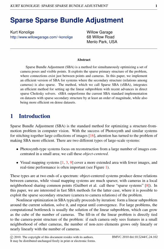
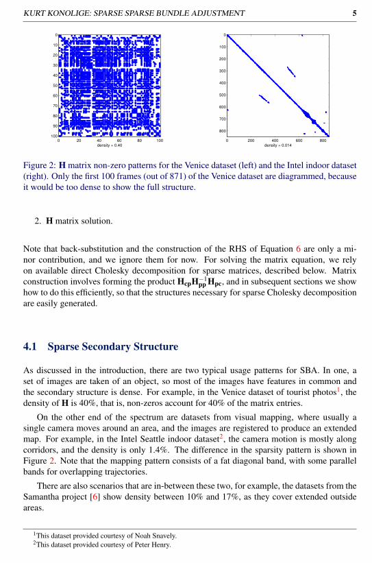
Figure 2: H matrix non-zero patterns for the Venice dataset (left) and the Intel indoor dataset(right). Only the first 100 frames (out of 871) of the Venice dataset are diagrammed, becauseit would be too dense to show the full structure.

2. H matrix solution.

Note that back-substitution and the construction of the RHS of Equation 6 are only a mi-nor contribution, and we ignore them for now. For solving the matrix equation, we relyon available direct Cholesky decomposition for sparse matrices, described below. Matrixconstruction involves forming the product HcpH−1

pp Hpc, and in subsequent sections we showhow to do this efficiently, so that the structures necessary for sparse Cholesky decompositionare easily generated.

4.1 Sparse Secondary Structure

As discussed in the introduction, there are two typical usage patterns for SBA. In one, aset of images are taken of an object, so most of the images have features in common andthe secondary structure is dense. For example, in the Venice dataset of tourist photos1, thedensity of H is 40%, that is, non-zeros account for 40% of the matrix entries.

On the other end of the spectrum are datasets from visual mapping, where usually asingle camera moves around an area, and the images are registered to produce an extendedmap. For example, in the Intel Seattle indoor dataset2, the camera motion is mostly alongcorridors, and the density is only 1.4%. The difference in the sparsity pattern is shown inFigure 2. Note that the mapping pattern consists of a fat diagonal band, with some parallelbands for overlapping trajectories.

There are also scenarios that are in-between these two, for example, the datasets from theSamantha project [6] show density between 10% and 17%, as they cover extended outsideareas.

1This dataset provided courtesy of Noah Snavely.2This dataset provided courtesy of Peter Henry.

6 KURT KONOLIGE: SPARSE SPARSE BUNDLE ADJUSTMENT

4.2 Compressed Column Storage

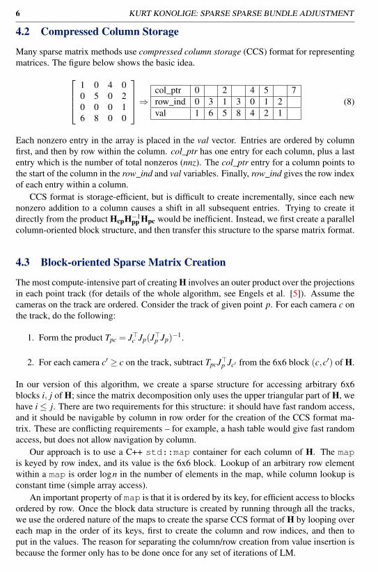
Many sparse matrix methods use compressed column storage (CCS) format for representingmatrices. The figure below shows the basic idea.

1 0 4 00 5 0 20 0 0 16 8 0 0

⇒ col_ptr 0 2 4 5 7row_ind 0 3 1 3 0 1 2val 1 6 5 8 4 2 1

(8)

Each nonzero entry in the array is placed in the val vector. Entries are ordered by columnfirst, and then by row within the column. col_ptr has one entry for each column, plus a lastentry which is the number of total nonzeros (nnz). The col_ptr entry for a column points tothe start of the column in the row_ind and val variables. Finally, row_ind gives the row indexof each entry within a column.

CCS format is storage-efficient, but is difficult to create incrementally, since each newnonzero addition to a column causes a shift in all subsequent entries. Trying to create itdirectly from the product HcpH−1

pp Hpc would be inefficient. Instead, we first create a parallelcolumn-oriented block structure, and then transfer this structure to the sparse matrix format.

4.3 Block-oriented Sparse Matrix Creation

The most compute-intensive part of creating H involves an outer product over the projectionsin each point track (for details of the whole algorithm, see Engels et al. [5]). Assume thecameras on the track are ordered. Consider the track of given point p. For each camera c onthe track, do the following:

1. Form the product Tpc = J>c Jp(J>p Jp)−1.

2. For each camera c′ ≥ c on the track, subtract TpcJ>p Jc′ from the 6x6 block (c,c′) of H.

In our version of this algorithm, we create a sparse structure for accessing arbitrary 6x6blocks i, j of H; since the matrix decomposition only uses the upper triangular part of H, wehave i≤ j. There are two requirements for this structure: it should have fast random access,and it should be navigable by column in row order for the creation of the CCS format ma-trix. These are conflicting requirements – for example, a hash table would give fast randomaccess, but does not allow navigation by column.

Our approach is to use a C++ std::map container for each column of H. The mapis keyed by row index, and its value is the 6x6 block. Lookup of an arbitrary row elementwithin a map is order logn in the number of elements in the map, while column lookup isconstant time (simple array access).

An important property of map is that it is ordered by its key, for efficient access to blocksordered by row. Once the block data structure is created by running through all the tracks,we use the ordered nature of the maps to create the sparse CCS format of H by looping overeach map in the order of its keys, first to create the column and row indices, and then toput in the values. The reason for separating the column/row creation from value insertion isbecause the former only has to be done once for any set of iterations of LM.

KURT KONOLIGE: SPARSE SPARSE BUNDLE ADJUSTMENT 7

4.4 ComplexityThe computational complexity for forming the H matrix depends on the average track size.In object-centered systems, the track size grows linearly with the number of frames N, soeach track is quadratic in N. The number of tracks stays constant or increases only slowly,since each new frame is connected to existing tracks; hence the complexity is order N2.Finally, the cost of insertion grows as logN, hence the total cost is N2 logN.

If the constraints are sparse as in mapping, the track size is bounded, so the computationfor each track is constant. The number of tracks grows linearly with N, since new tracksappear at a constant rate. Insertion cost is constant, because the average map size is constant.The total complexity is thus order N, which is lower than for object-centered systems.

4.5 Sparse Linear SystemsFor solving (4) in sparse format, we use the CHOLMOD package [4]. This package has ahighly-optimized Cholesky decomposition solver for sparse linear systems. It employs sev-eral strategies to decompose H efficiently, including a logical ordering and an approximateminimal degree (AMD) algorithm to reorder variables when H is large.

In general the complexity of decomposition will be O(n3) in the number of variables.For sparse matrices, the complexity will depend on the density of the Cholesky factor, whichin turn depends on the structure of H and the order of its variables. Mahon et al. [13] haveanalyzed the behavior of the Cholesky factorization as a function of the loop closures in theSLAM system. If the number of loop closures is constant, then the Cholesky factor densityis O(n), and decomposition is O(n). If the number of loop closures grows linearly with thenumber of variables, then the Cholesky factor density grows as O(n2) and decomposition isO(n3).

5 ExperimentsTo exercise sSBA, we performed experiments on both synthetic and real datasets. Withsynthetic datasets, it is possible to perform extensive experiments and to isolate the effect ofvariables on performance. Real datasets verify the conclusions of the synthetic datasets, andshow the system functioning in real-world situations.

5.1 Lourakis and Argyros SBAIn the experiments, we compared sSBA against the system of Lourakis and Argyros [11](laSBA), which is the standard open-source SBA system in the vision community. laSBAperforms the same operations as sSBA: H-matrix formation, H-matrix solution, and back-substitution. Like sSBA, it uses unit quaternions and local angle representations. Finally,similar to sSBA, laSBA stores only non-zero Hi j blocks. The major differences betweenlaSBA and sSBA are:

1. laSBA uses a compressed row storage (CRS) format for indexing, rather than the mapdata structure.

2. laSBA does not use the track-oriented algorithm for decomposing HcpH−1pp Hpc in

forming H.

8 KURT KONOLIGE: SPARSE SPARSE BUNDLE ADJUSTMENT

0 2000 4000 6000 8000 1000010

−1

100

101

102

103

104

Number of cameras

Tim

e p

er

itera

tion, s

Nc = 25

sSBA

dSBA

laSBA

0 2000 4000 6000 8000 1000010

−1

100

101

102

103

104

Number of cameras

Tim

e p

er

itera

tion, s

Nc = 138

sSBA

dSBA

laSBA

0 10 20 30 40 5010

0

101

102

103

H matrix density, percent

laS

BA

/sS

BA

tim

e p

er

itera

tion

Relative timing vs. connection density

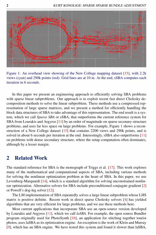
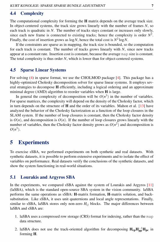
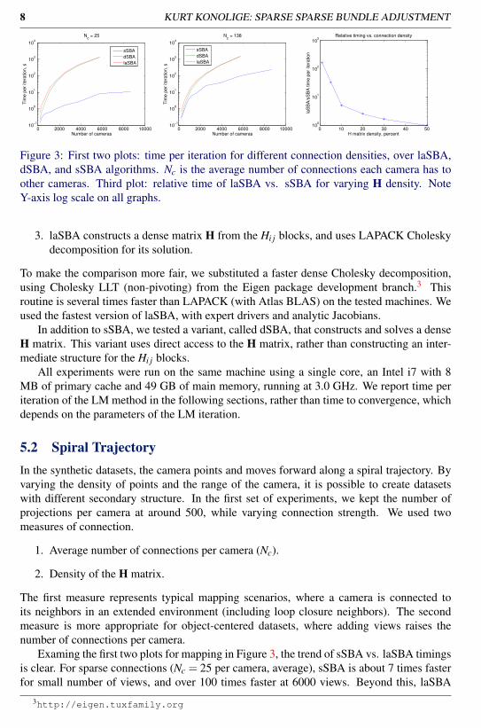
Figure 3: First two plots: time per iteration for different connection densities, over laSBA,dSBA, and sSBA algorithms. Nc is the average number of connections each camera has toother cameras. Third plot: relative time of laSBA vs. sSBA for varying H density. NoteY-axis log scale on all graphs.

3. laSBA constructs a dense matrix H from the Hi j blocks, and uses LAPACK Choleskydecomposition for its solution.

To make the comparison more fair, we substituted a faster dense Cholesky decomposition,using Cholesky LLT (non-pivoting) from the Eigen package development branch.3 Thisroutine is several times faster than LAPACK (with Atlas BLAS) on the tested machines. Weused the fastest version of laSBA, with expert drivers and analytic Jacobians.

In addition to sSBA, we tested a variant, called dSBA, that constructs and solves a denseH matrix. This variant uses direct access to the H matrix, rather than constructing an inter-mediate structure for the Hi j blocks.

All experiments were run on the same machine using a single core, an Intel i7 with 8MB of primary cache and 49 GB of main memory, running at 3.0 GHz. We report time periteration of the LM method in the following sections, rather than time to convergence, whichdepends on the parameters of the LM iteration.

5.2 Spiral TrajectoryIn the synthetic datasets, the camera points and moves forward along a spiral trajectory. Byvarying the density of points and the range of the camera, it is possible to create datasetswith different secondary structure. In the first set of experiments, we kept the number ofprojections per camera at around 500, while varying connection strength. We used twomeasures of connection.

1. Average number of connections per camera (Nc).

2. Density of the H matrix.

The first measure represents typical mapping scenarios, where a camera is connected toits neighbors in an extended environment (including loop closure neighbors). The secondmeasure is more appropriate for object-centered datasets, where adding views raises thenumber of connections per camera.

Examing the first two plots for mapping in Figure 3, the trend of sSBA vs. laSBA timingsis clear. For sparse connections (Nc = 25 per camera, average), sSBA is about 7 times fasterfor small number of views, and over 100 times faster at 6000 views. Beyond this, laSBA

3http://eigen.tuxfamily.org

KURT KONOLIGE: SPARSE SPARSE BUNDLE ADJUSTMENT 9

0 2000 4000 6000 8000 100000

50

100

150

200

250

300

Number of cameras

Tim

e p

er

ite

ratio

n,

sN

c = 138

sSBA

laSBA

3000

1500

3000

1500

500

1000

1000

500

200 400 600 800 1000 1200 1400 1600 1800 2000 220010

−1

100

101

102

103

Timing per iteration for New College dataset

Number of cameras

Tim

e p

er

ite

ratio

n,

s

laSBA

sSBA

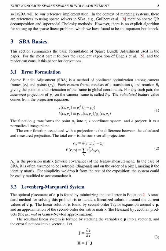
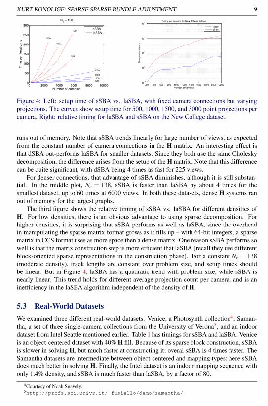
Figure 4: Left: setup time of sSBA vs. laSBA, with fixed camera connections but varyingprojections. The curves show setup time for 500, 1000, 1500, and 3000 point projections percamera. Right: relative timing for laSBA and sSBA on the New College dataset.

runs out of memory. Note that sSBA trends linearly for large number of views, as expectedfrom the constant number of camera connections in the H matrix. An interesting effect isthat dSBA out-performs laSBA for smaller datasets. Since they both use the same Choleskydecomposition, the difference arises from the setup of the H matrix. Note that this differencecan be quite significant, with dSBA being 4 times as fast for 225 views.

For denser connections, that advantage of sSBA diminishes, although it is still substan-tial. In the middle plot, Nc = 138, sSBA is faster than laSBA by about 4 times for thesmallest dataset, up to 60 times at 6000 views. In both these datasets, dense H systems ranout of memory for the largest graphs.

The third figure shows the relative timing of sSBA vs. laSBA for different densities ofH. For low densities, there is an obvious advantage to using sparse decomposition. Forhigher densities, it is surprising that sSBA performs as well as laSBA, since the overheadin manipulating the sparse matrix format grows as it fills up – with 64-bit integers, a sparsematrix in CCS format uses as more space then a dense matrix. One reason sSBA performs sowell is that the matrix construction step is more efficient that laSBA (recall they use differentblock-oriented sparse representations in the construction phase). For a constant Nc = 138(moderate density), track lengths are constant over problem size, and setup times shouldbe linear. But in Figure 4, laSBA has a quadratic trend with problem size, while sSBA isnearly linear. This trend holds for different average projection count per camera, and is aninefficiency in the laSBA algorithm independent of the density of H.

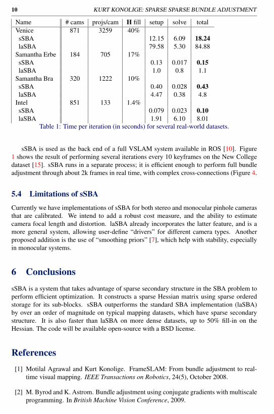
5.3 Real-World DatasetsWe examined three different real-world datasets: Venice, a Photosynth collection4; Saman-tha, a set of three single-camera collections from the University of Verona5, and an indoordataset from Intel Seattle mentioned earlier. Table 1 has timings for sSBA and laSBA. Veniceis an object-centered dataset with 40% H fill. Because of its sparse block construction, sSBAis slower in solving H, but much faster at constructing it; overal sSBA is 4 times faster. TheSamantha datasets are intermediate between object-centered and mapping types; here sSBAdoes much better in solving H. Finally, the Intel dataset is an indoor mapping sequence withonly 1.4% density, and sSBA is much faster than laSBA, by a factor of 80.

4Courtesy of Noah Snavely.5http://profs.sci.univr.it/ fusiello/demo/samantha/

10 KURT KONOLIGE: SPARSE SPARSE BUNDLE ADJUSTMENT

Name # cams projs/cam H fill setup solve totalVenice 871 3259 40%sSBA 12.15 6.09 18.24laSBA 79.58 5.30 84.88

Samantha Erbe 184 705 17%sSBA 0.13 0.017 0.15laSBA 1.0 0.8 1.1

Samantha Bra 320 1222 10%sSBA 0.40 0.028 0.43laSBA 4.47 0.38 4.8

Intel 851 133 1.4%sSBA 0.079 0.023 0.10laSBA 1.91 6.10 8.01

Table 1: Time per iteration (in seconds) for several real-world datasets.

sSBA is used as the back end of a full VSLAM system available in ROS [10]. Figure1 shows the result of performing several iterations every 10 keyframes on the New Collegedataset [15]. sSBA runs in a separate process; it is efficient enough to perform full bundleadjustment through about 2k frames in real time, with complex cross-connections (Figure 4.

5.4 Limitations of sSBA

Currently we have implementations of sSBA for both stereo and monocular pinhole camerasthat are calibrated. We intend to add a robust cost measure, and the ability to estimatecamera focal length and distortion. laSBA already incorporates the latter feature, and is amore general system, allowing user-define “drivers” for different camera types. Anotherproposed addition is the use of “smoothing priors” [7], which help with stability, especiallyin monocular systems.

6 Conclusions

sSBA is a system that takes advantage of sparse secondary structure in the SBA problem toperform efficient optimization. It constructs a sparse Hessian matrix using sparse orderedstorage for its sub-blocks. sSBA outperforms the standard SBA implementation (laSBA)by over an order of magnitude on typical mapping datasets, which have sparse secondarystructure. It is also faster than laSBA on more dense datasets, up to 50% fill-in on theHessian. The code will be available open-source with a BSD license.

References[1] Motilal Agrawal and Kurt Konolige. FrameSLAM: From bundle adjustment to real-

time visual mapping. IEEE Transactions on Robotics, 24(5), October 2008.

[2] M. Byrod and K. Astrom. Bundle adjustment using conjugate gradients with multiscaleprogramming. In British Machine Vision Conference, 2009.

KURT KONOLIGE: SPARSE SPARSE BUNDLE ADJUSTMENT 11

[3] Mark Cummins and Paul M. Newman. Highly scalable appearance-only SLAM – FAB-MAP 2.0. In Robotics Science and Systems, 2009.

[4] Timothy A. Davis. Direct Methods for Sparse Linear Systems (Fundamentals of Al-gorithms 2). Society for Industrial and Applied Mathematics, Philadelphia, PA, USA,2006.

[5] Chris Engels, Henrik Stewénius, and David Nister. Bundle adjustment rules. Pho-togrammetric Computer Vision, September 2006.

[6] M. Farenzena, A. Fusiello, and R. Gherardi. Structure-and-motion pipeline on a hier-archical cluster tree. In ICCV Workshop on 3-D Digital Imaging and Modeling, pages1489–1496, 2009.

[7] Michela Farenzena, Adrien Bartoli, and Youcef Mezouar. Efficient camera smoothingin sequential structure-from-motion using approximate cross-validation. In ECCV (3),pages 196–209, 2008.

[8] Nicolas Guilbert, Adrien Bartoli, and Anders Heyden. Affine approximation for directbatch recovery of euclidian structure and motion from sparse data. Int. J. Comput.Vision, 69(3):317–333, 2006.

[9] Georg Klein and David Murray. Parallel tracking and mapping for small ARworkspaces. In Proc. Sixth IEEE and ACM International Symposium on Mixed andAugmented Reality (ISMAR’07), Nara, Japan, November 2007.

[10] K. Konolige. Vslam package. Willow Garage, Robot Operating System, WG-ROS-PKG, SVN Repository, 2010. Available online at https://code.ros.org/svn/wg-ros-pkg/trunk/vision/vslam_system.

[11] M.I. A. Lourakis and A.A. Argyros. SBA: A Software Package for Generic SparseBundle Adjustment. ACM Trans. Math. Software, 36(1):1–30, 2009.

[12] M.I.A. Lourakis and A.A. Argyros. Is levenberg-marquardt the most efficient optimiza-tion algorithm for implementing bundle adjustment? In Proc. International Conferenceon Computer Vision, 2005.

[13] I.J. Mahon, S.B. Williams, O. Pizarro, and M. Johnson-Roberson. Efficient view-basedSLAM using visual loop closures. IEEE Transactions on Robotics, 24(5):1002–1014,October 2008.

[14] Donald W. Marquardt. An algorithm for least-squares estimation of nonlinear parame-ters. SIAM Journal on Applied Mathematics, 11(2):431–441, 1963.

[15] M. Smith, I. Baldwin, W. Churchill, R. Paul, and P. Newman. The new college visionand laser data set. International Journal for Robotics Research (IJRR), 28(5):595–599,May 2009. ISSN 0278-3649.

[16] Noah Snavely, Steven M. Seitz, and Richard Szeliski. Skeletal sets for efficient struc-ture from motion. In Conference on Computer Vision and Pattern Recognition, 2008.

[17] B. Triggs, P. F. McLauchlan, R. I. Hartley, and A. W. Fitzibbon. Bundle adjustment - amodern synthesis. In Vision Algorithms: Theory and Practice, LNCS, pages 298–375.Springer Verlag, 2000.