Spatial Access MethodsSpatial Access Methods

Chapter 26 of bookRead only 26.1, 26.2, 26.6

Dr Eamonn KeoghDr Eamonn KeoghComputer Science & Engineering Department

University of California - RiversideRiverside,CA 92521eamonn@cs.ucr.edu

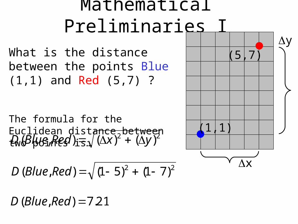
Mathematical Preliminaries I

(1,1)

What is the distance between the points Blue (1,1) and Red (5,7) ?

The formula for the Euclidean distance between two points is…

22 )()(),( yxedRBlueD

22 )71()51(),( edRBlueD

(5,7)

21.7),( edRBlueD

x

y

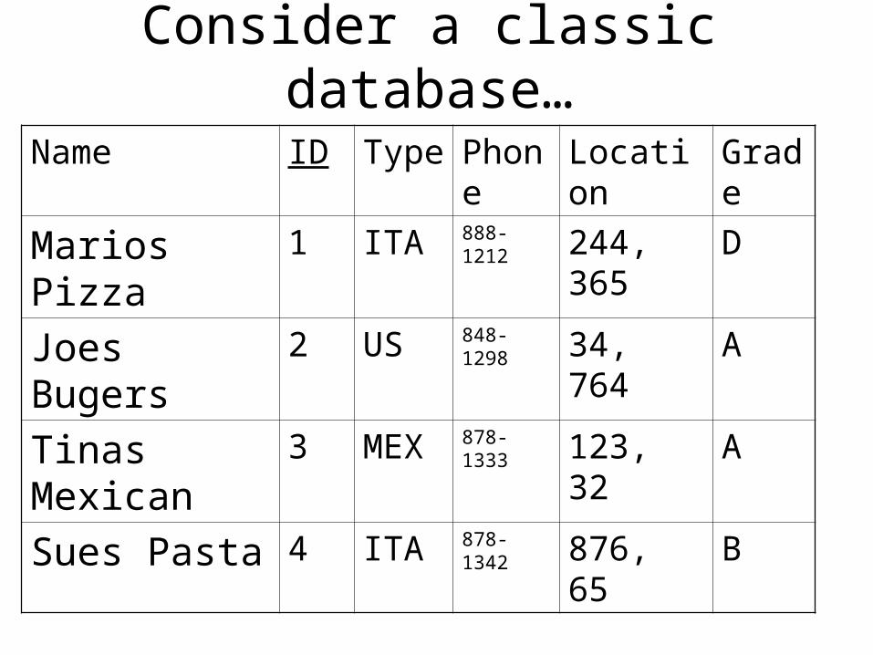
Consider a classic database…

Name ID Type Phone Location Grade

Marios Pizza 1 ITA 888-1212 244, 365 D

Joes Bugers 2 US 848-1298 34, 764 A

Tinas Mexican 3 MEX 878-1333 123, 32 A

Sues Pasta 4 ITA 878-1342 876, 65 B

B876,65878-1342ITA4Sues Pasta

A123,32878-1333MEX3Tinas Mexican

A34,764848-1298US2Joes Bugers

D244,365888-1212ITA1Marios Pizza

GradeLocationPhoneTypeIDName

B876,65878-1342ITA4Sues Pasta

A123,32878-1333MEX3Tinas Mexican

A34,764848-1298US2Joes Bugers

D244,365888-1212ITA1Marios Pizza

GradeLocationPhoneTypeIDName

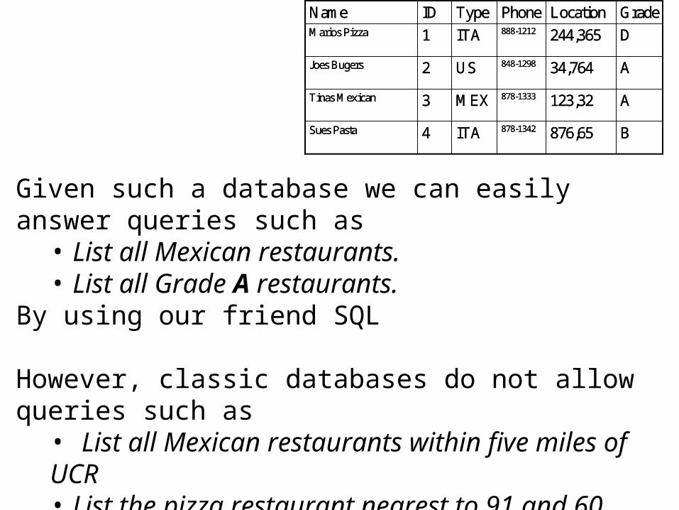
Given such a database we can easily answer queries such as• List all Mexican restaurants.• List all Grade A restaurants.

By using our friend SQL

However, classic databases do not allow queries such as• List all Mexican restaurants within five miles of UCR• List the pizza restaurant nearest to 91 and 60.

These kinds of queries are called spatial queries.

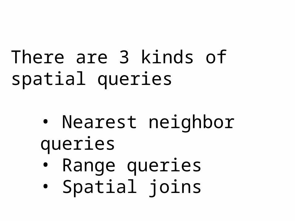
There are 3 kinds of spatial queries

• Nearest neighbor queries • Range queries • Spatial joins

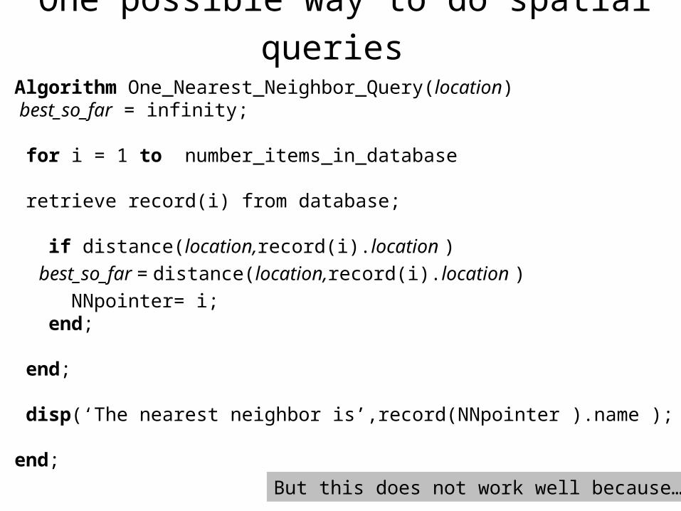
One possible way to do spatial queries Algorithm One_Nearest_Neighbor_Query(location) best_so_far = infinity;

for i = 1 to number_items_in_database

retrieve record(i) from database;

if distance(location,record(i).location )

best_so_far = distance(location,record(i).location )

NNpointer= i; end;

end;

disp(‘The nearest neighbor is’,record(NNpointer ).name );

end;

But this does not work well because…

…so we need to index the data

As we have seen in detail, indexing some kinds of data is trivial…

My informal definition of indexing. Organizing the data such that queries can be answered in sub linear time.

So, we call always index 1-dimensional data (if you can sort it, you can index it), such that we can answer 1-nearest neighbor queries by accessing just O(log(n) ) of the database. (n is the number of items in the database).

(i.e. the B+tree)

But we can’t sort 2 dimensional data…

This is an important problem which has attracted a great deal of research interest….

We can in fact index 2 (and higher) dimensional reasonably efficiently with special data structures known as Spatial Access Methods (SAM) or Multidimensional Access Methods.

Although there are many variations we will focus on the R-Tree, introduced by Guttman in the 1984 SIGMOD conference.

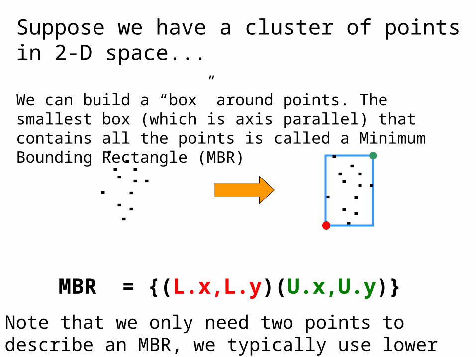
Suppose we have a cluster of points in 2-D space...

We can build a “box” around points. The smallest box (which is axis parallel) that contains all the points is called a Minimum Bounding Rectangle (MBR)

Note that we only need two points to describe an MBR, we typically use lower left, and upper right.

MBR = {(L.x,L.y)(U.x,U.y)}

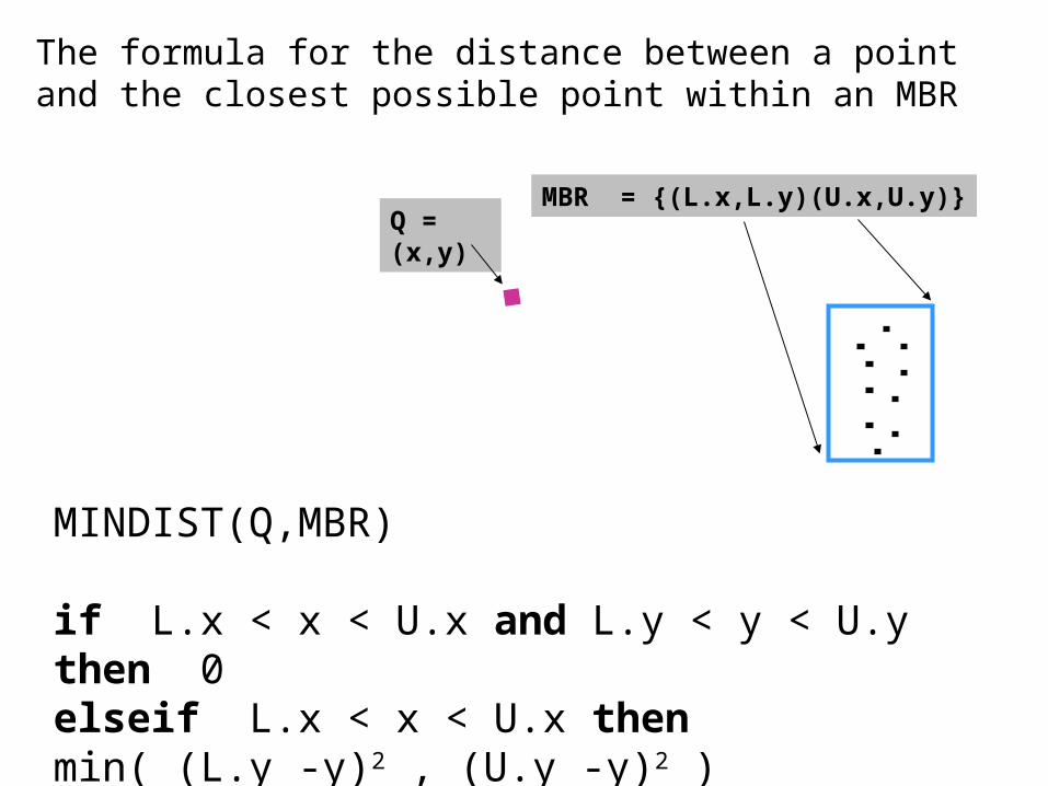
The formula for the distance between a point and the closest possible point within an MBR

MBR = {(L.x,L.y)(U.x,U.y)}

MINDIST(Q,MBR)

if L.x < x < U.x and L.y < y < U.y then 0elseif L.x < x < U.x then min( (L.y -y)2 , (U.y -y)2 )elseif ….

Q = (x,y)

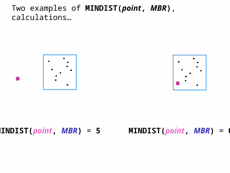
Two examples of MINDIST(point, MBR), calculations…

MINDIST(point, MBR) = 5 MINDIST(point, MBR) = 0

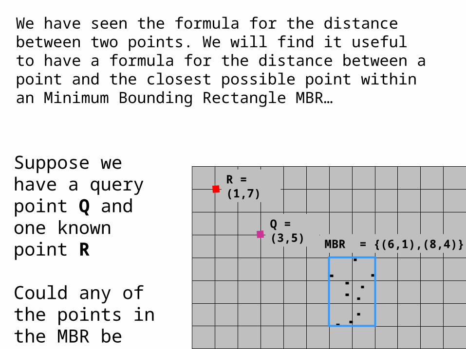
We have seen the formula for the distance between two points. We will find it useful to have a formula for the distance between a point and the closest possible point within an Minimum Bounding Rectangle MBR…

MBR = {(6,1),(8,4)}

Q = (3,5)

R = (1,7)Suppose we have a query point Q and one known point R

Could any of the points in the MBR be closer to Q than R is?

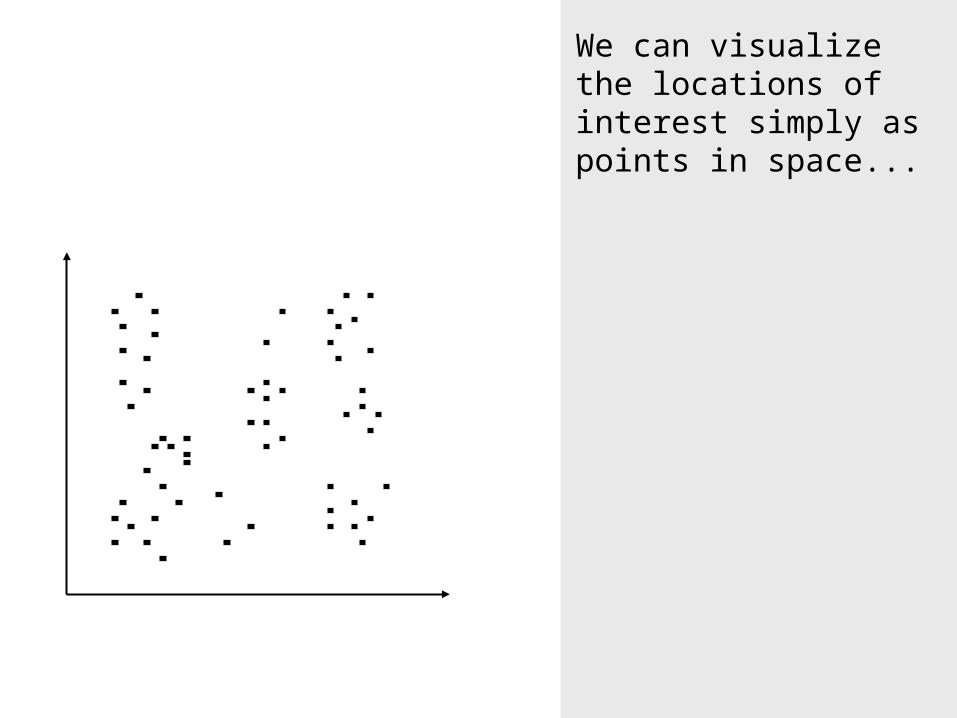
We can visualize the locations of interest simply as points in space...

R1

R2R5

R3

R7R9

R8

R6

R4

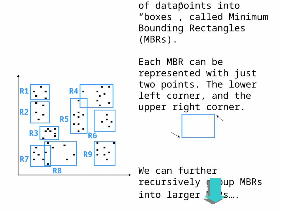
We can group clusters of datapoints into “boxes”, called Minimum Bounding Rectangles (MBRs).

Each MBR can be represented with just two points. The lower left corner, and the upper right corner.

We can further recursively group MBRs into larger MBRs….

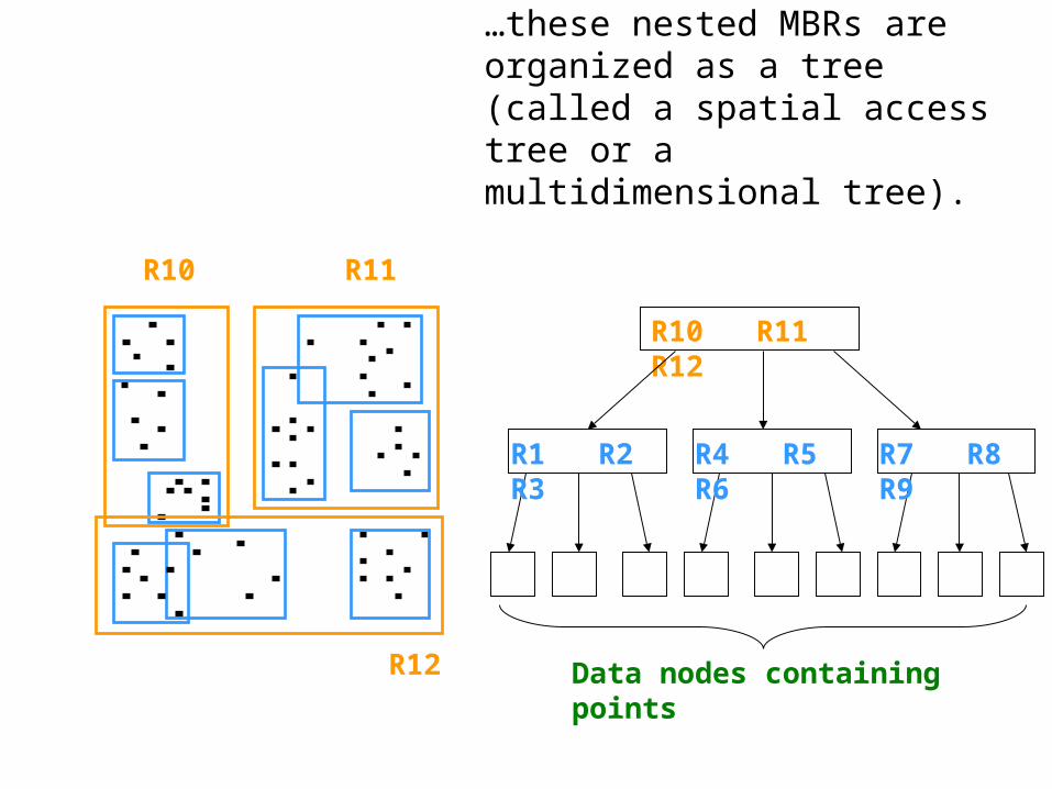
R10 R11 R12

R1 R2 R3 R4 R5 R6 R7 R8 R9

Data nodes containing points

R10 R11

R12

…these nested MBRs are organized as a tree (called a spatial access tree or a multidimensional tree).

R10

R1 R2 R3

Data nodes

R12

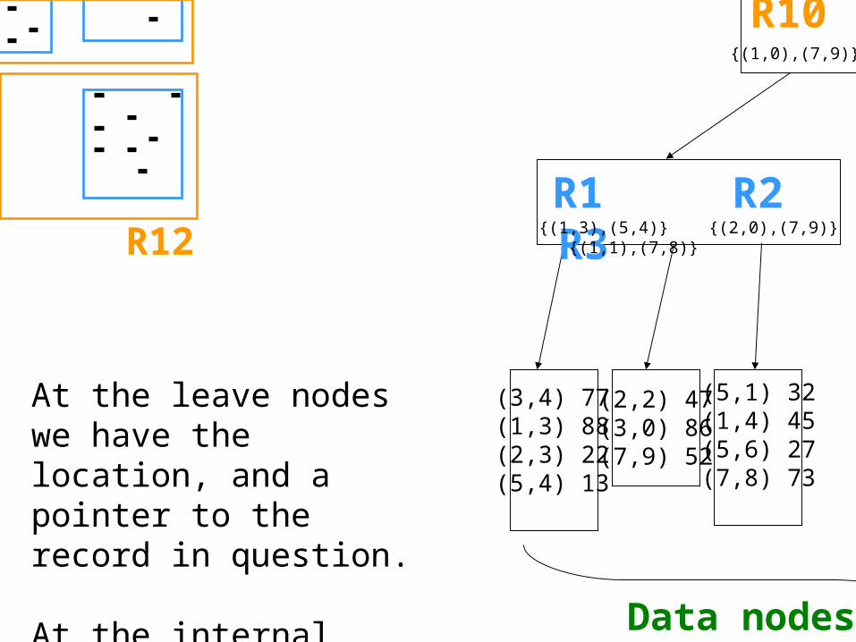
(3,4) 77(1,3) 88(2,3) 22(5,4) 13

(2,2) 47(3,0) 86(7,9) 52

(5,1) 32(1,4) 45(5,6) 27(7,8) 73

{(1,3),(5,4)} {(2,0),(7,9)} {(1,1),(7,8)}

{(1,0),(7,9)}

At the leave nodes we have the location, and a pointer to the record in question.

At the internal nodes, we just have MBR information.

R-TreesR-Trees• R-trees are a N-dimensional extension of B+-trees,

useful for indexing sets of rectangles and other polygons.

• Supported in many modern database systems, along with variants like R+ -trees and R*-trees.

• Basic idea: generalize the notion of a one-dimensional interval associated with each B+ -tree node to an N-dimensional interval, that is, an N-dimensional rectangle.

• Will consider only the two-dimensional case (N = 2) – generalization for N > 2 is straightforward, although R-trees

work well only for relatively small N

R Trees (Cont.)R Trees (Cont.)• A rectangular bounding box is associated with each tree

node.– Bounding box of a leaf node is a minimum sized rectangle that

contains all the rectangles/polygons associated with the leaf node.

– The bounding box associated with a non-leaf node contains the bounding box associated with all its children.

– Bounding box of a node serves as its key in its parent node (if any)

– Bounding boxes of children of a node are allowed to overlap

• A polygon is stored only in one node, and the bounding box of the node must contain the polygon– The storage efficiency or R-trees is better than that of k-d trees

or quadtrees since a polygon is stored only once

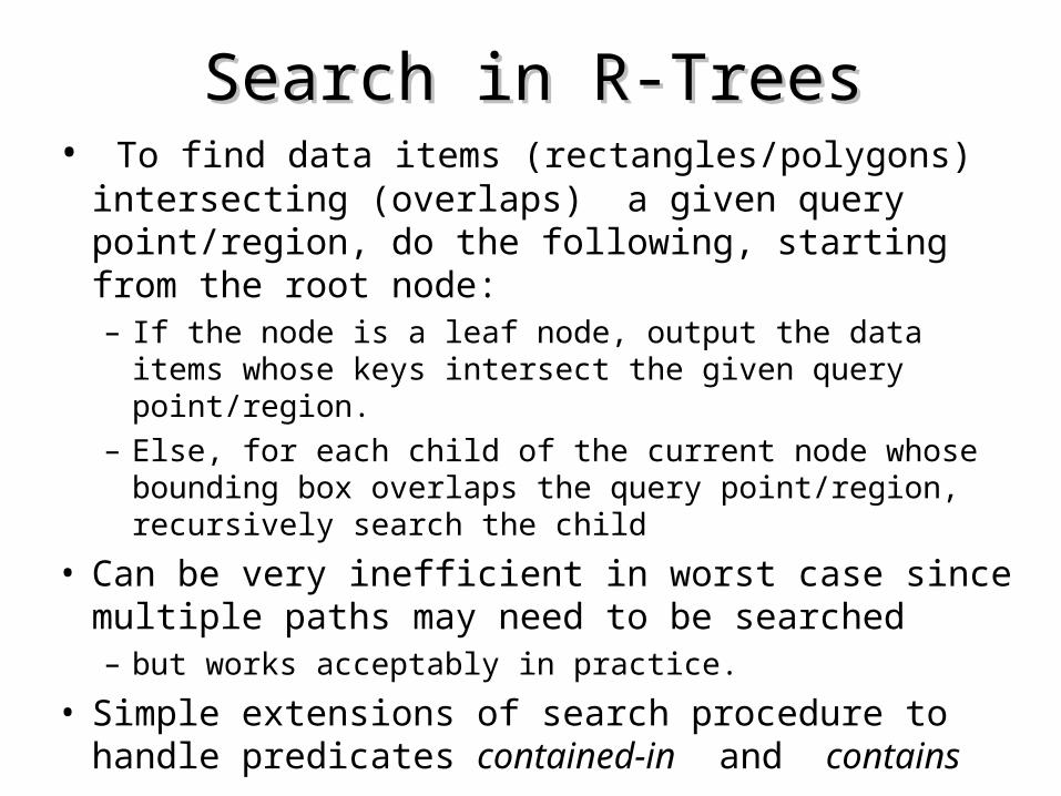
Search in R-TreesSearch in R-Trees• To find data items (rectangles/polygons) intersecting

(overlaps) a given query point/region, do the following, starting from the root node:– If the node is a leaf node, output the data items whose keys

intersect the given query point/region.

– Else, for each child of the current node whose bounding box overlaps the query point/region, recursively search the child

• Can be very inefficient in worst case since multiple paths may need to be searched– but works acceptably in practice.

• Simple extensions of search procedure to handle predicates contained-in and contains

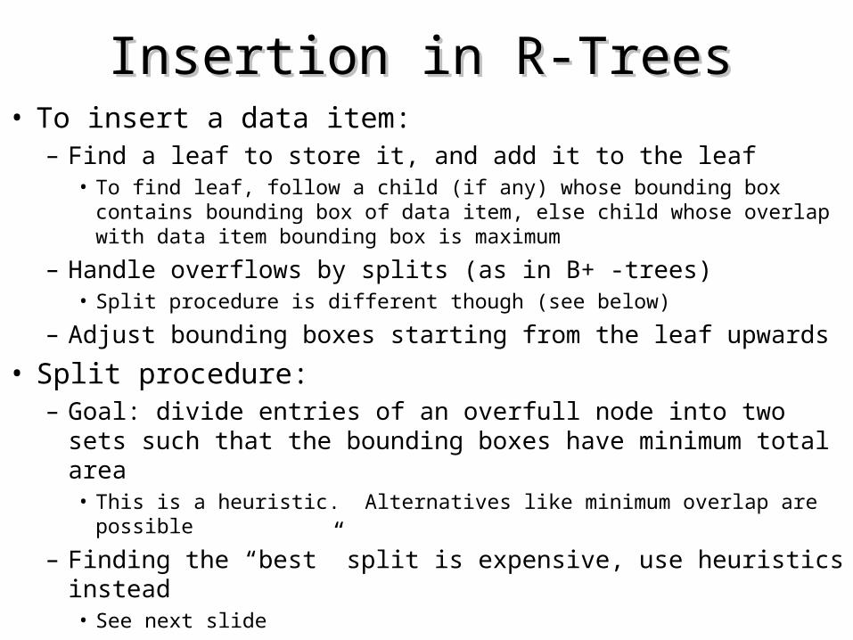
Insertion in R-TreesInsertion in R-Trees• To insert a data item:

– Find a leaf to store it, and add it to the leaf• To find leaf, follow a child (if any) whose bounding box contains bounding

box of data item, else child whose overlap with data item bounding box is maximum

– Handle overflows by splits (as in B+ -trees) • Split procedure is different though (see below)

– Adjust bounding boxes starting from the leaf upwards

• Split procedure:– Goal: divide entries of an overfull node into two sets such that the

bounding boxes have minimum total area • This is a heuristic. Alternatives like minimum overlap are possible

– Finding the “best” split is expensive, use heuristics instead• See next slide

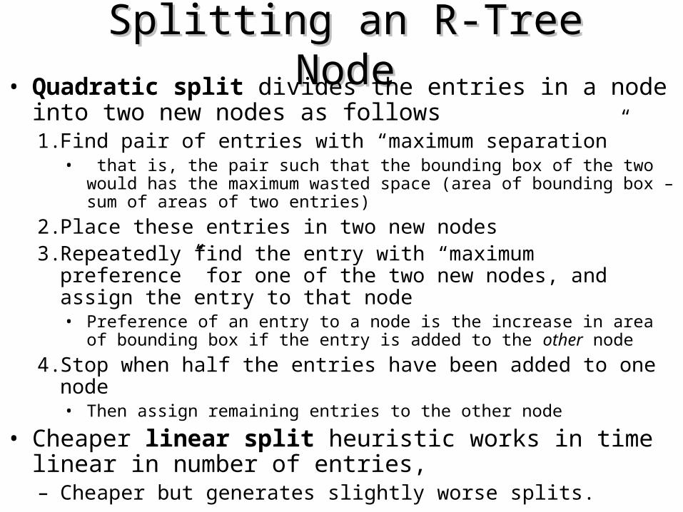
Splitting an R-Tree NodeSplitting an R-Tree Node• Quadratic split divides the entries in a node into two new

nodes as follows1. Find pair of entries with “maximum separation”

• that is, the pair such that the bounding box of the two would has the maximum wasted space (area of bounding box – sum of areas of two entries)

2. Place these entries in two new nodes3. Repeatedly find the entry with “maximum preference” for one of

the two new nodes, and assign the entry to that node• Preference of an entry to a node is the increase in area of bounding box if

the entry is added to the other node

4. Stop when half the entries have been added to one node• Then assign remaining entries to the other node

• Cheaper linear split heuristic works in time linear in number of entries,– Cheaper but generates slightly worse splits.

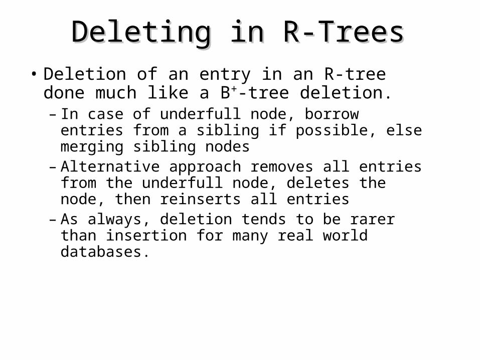
Deleting in R-TreesDeleting in R-Trees

• Deletion of an entry in an R-tree done much like a B+-tree deletion.– In case of underfull node, borrow entries from a

sibling if possible, else merging sibling nodes– Alternative approach removes all entries from

the underfull node, deletes the node, then reinserts all entries

– As always, deletion tends to be rarer than insertion for many real world databases.