Spatial Analyst is an extension in ArcGIS specially designed for working with raster data.

1

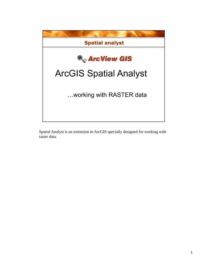
In Lesson 2 you learned about the difference between vector and raster data. Vector data representations are points, lines and polygons, while raster data is composed of pixels (cells) of a certain size. So far in this class we have worked with the vector data tools, however today’s lesson and exercise will cover raster data tools. It is important to be aware of the fact different analysis tools in ArcGIS are used for vector and raster data.This slide shows three raster data layers. 1) an ArcInfo GRID displaying the y ) p y glandcover types of Latah county, Idaho. The brown pixels represent agricultural lands while the green and yellow pixels represent forested lands. 2) a black&white aerial photograph – if you zoom in far enough on any photograph you will see that it is made up of pixels. 3) a digital elevation model (DEM) for Latah county, Idaho where each pixel value represents the elevation at that particular location – in this DEM the light colors represent high elevation and the dark areas represent low elevation.

2

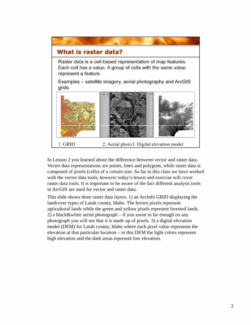
Satellite imagery is raster data. These are clips from Landsat 7 imagery at 30 meter pixel size.

3

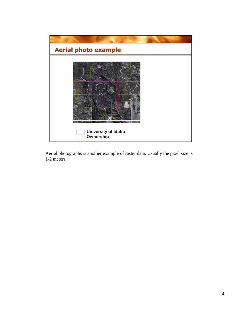
Aerial photographs is another example of raster data. Usually the pixel size is 1-2 meters.

4

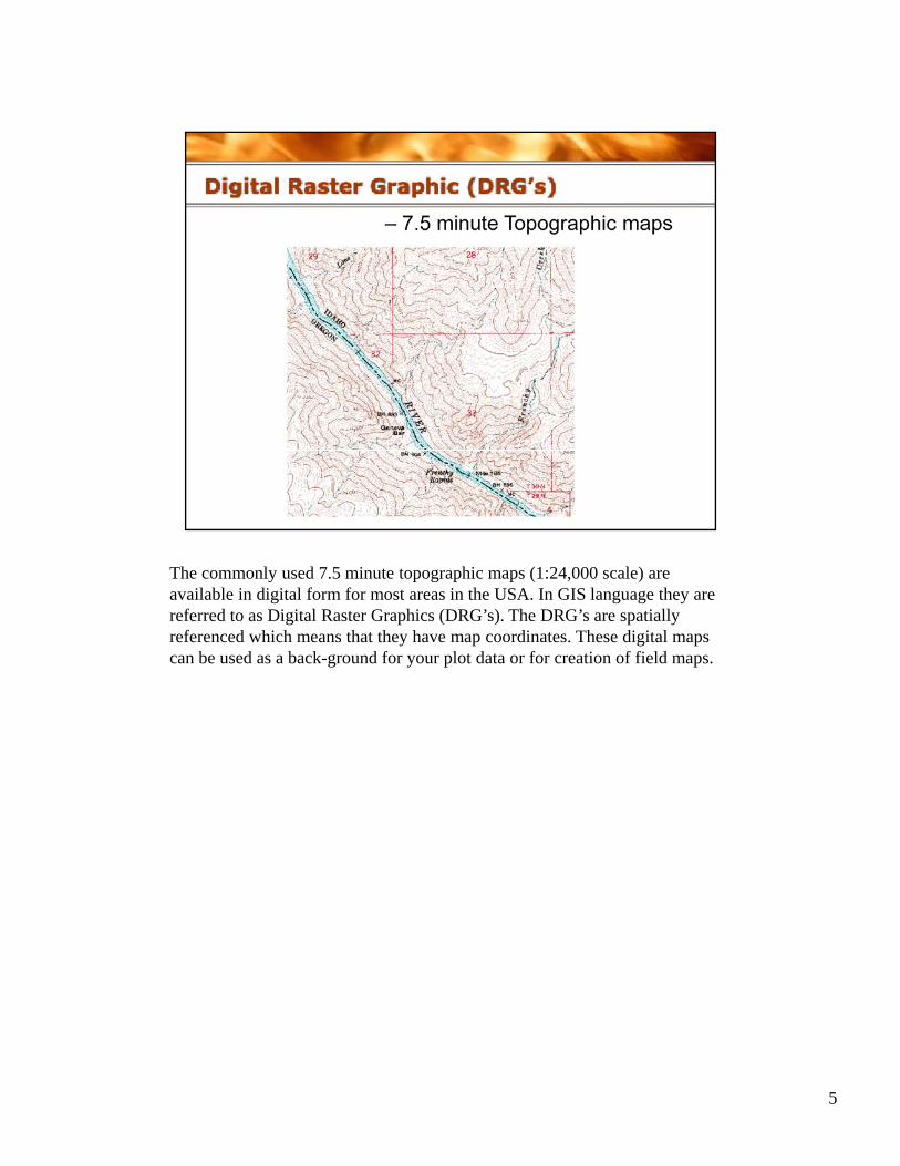
The commonly used 7.5 minute topographic maps (1:24,000 scale) are available in digital form for most areas in the USA. In GIS language they are referred to as Digital Raster Graphics (DRG’s). The DRG’s are spatially referenced which means that they have map coordinates. These digital maps can be used as a back-ground for your plot data or for creation of field maps.

5

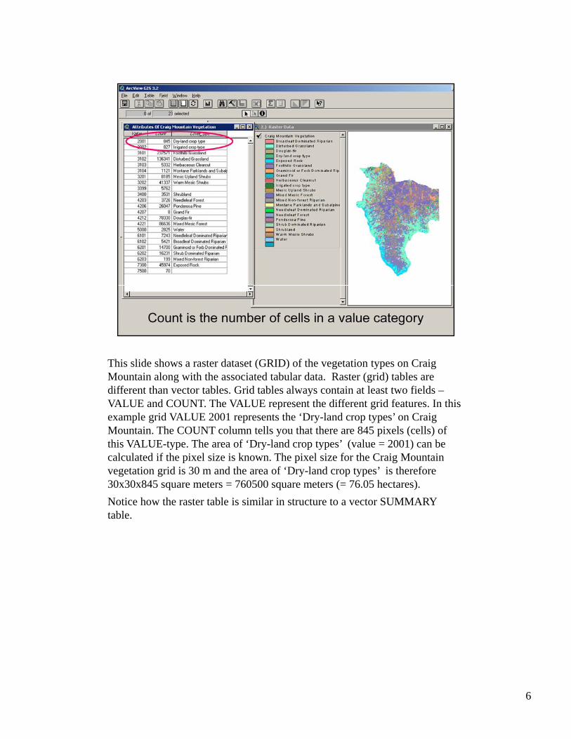
This slide shows a raster dataset (GRID) of the vegetation types on Craig Mountain along with the associated tabular data. Raster (grid) tables are different than vector tables. Grid tables always contain at least two fields –VALUE and COUNT. The VALUE represent the different grid features. In this example grid VALUE 2001 represents the ‘Dry-land crop types’ on Craig Mountain. The COUNT column tells you that there are 845 pixels (cells) of this VALUE-type. The area of ‘Dry-land crop types’ (value = 2001) can be

l l d if h i l i i k h i l i f h C i icalculated if the pixel size is known. The pixel size for the Craig Mountain vegetation grid is 30 m and the area of ‘Dry-land crop types’ is therefore 30x30x845 square meters = 760500 square meters (= 76.05 hectares).Notice how the raster table is similar in structure to a vector SUMMARY table.

6

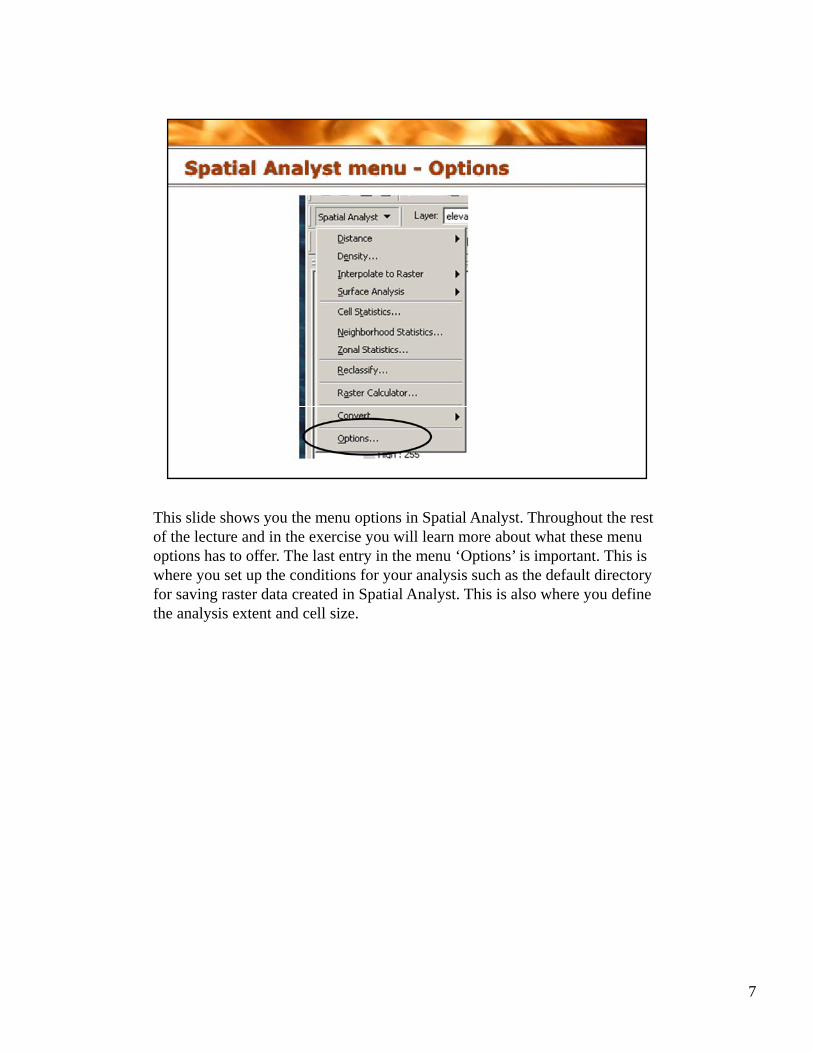
This slide shows you the menu options in Spatial Analyst. Throughout the rest of the lecture and in the exercise you will learn more about what these menu options has to offer. The last entry in the menu ‘Options’ is important. This is where you set up the conditions for your analysis such as the default directory for saving raster data created in Spatial Analyst. This is also where you define the analysis extent and cell size.

7

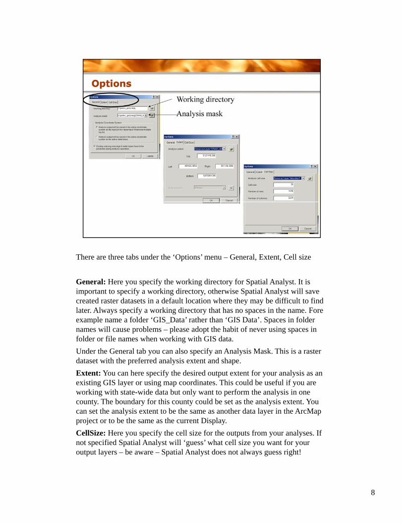
There are three tabs under the ‘Options’ menu – General, Extent, Cell size

General: Here you specify the working directory for Spatial Analyst. It is important to specify a working directory, otherwise Spatial Analyst will save created raster datasets in a default location where they may be difficult to find later. Always specify a working directory that has no spaces in the name. Fore example name a folder ‘GIS Data’ rather than ‘GIS Data’ Spaces in folderexample name a folder GIS_Data rather than GIS Data . Spaces in folder names will cause problems – please adopt the habit of never using spaces in folder or file names when working with GIS data.Under the General tab you can also specify an Analysis Mask. This is a raster dataset with the preferred analysis extent and shape.Extent: You can here specify the desired output extent for your analysis as an

i i GIS l i di Thi ld b f l ifexisting GIS layer or using map coordinates. This could be useful if you are working with state-wide data but only want to perform the analysis in one county. The boundary for this county could be set as the analysis extent. You can set the analysis extent to be the same as another data layer in the ArcMap project or to be the same as the current Display.CellSize: Here you specify the cell size for the outputs from your analyses. If

ifi d S i l A l ill ‘ ’ h ll i f

8

not specified Spatial Analyst will ‘guess’ what cell size you want for your output layers – be aware – Spatial Analyst does not always guess right!

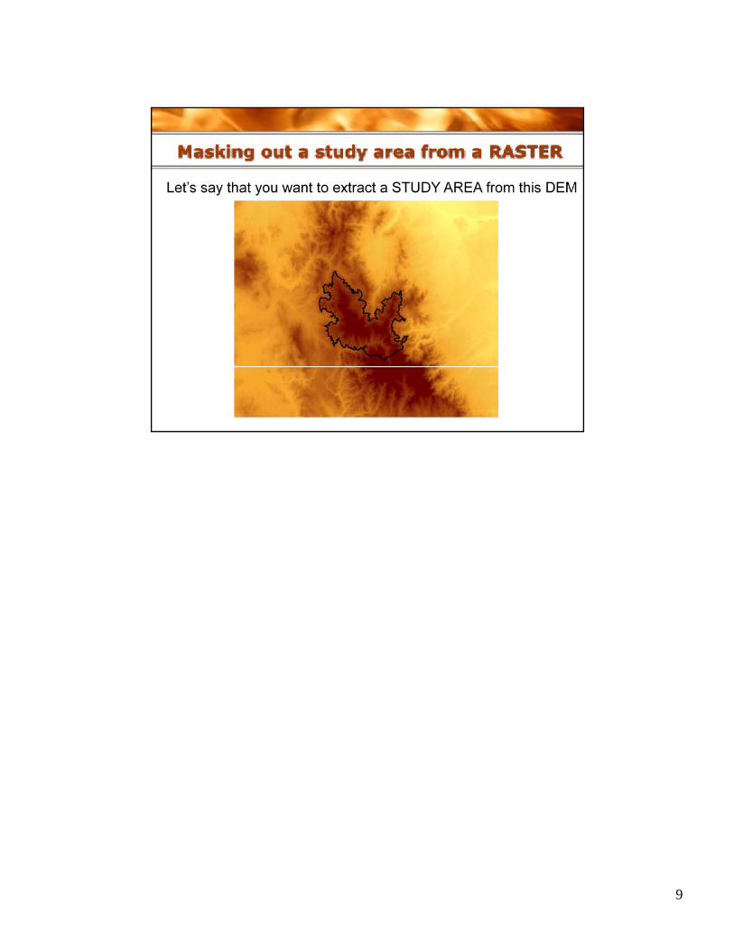
9

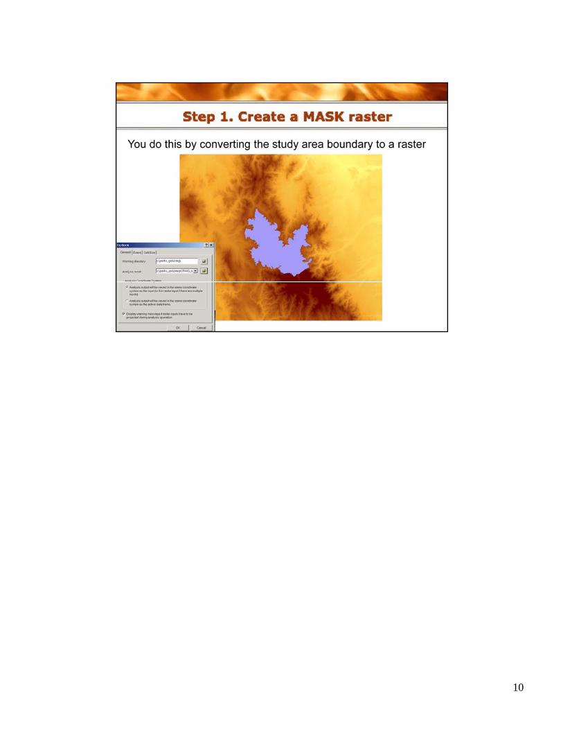
10

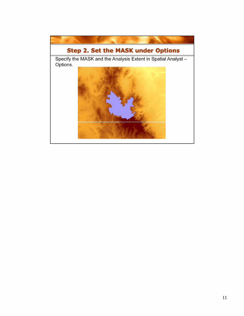
11

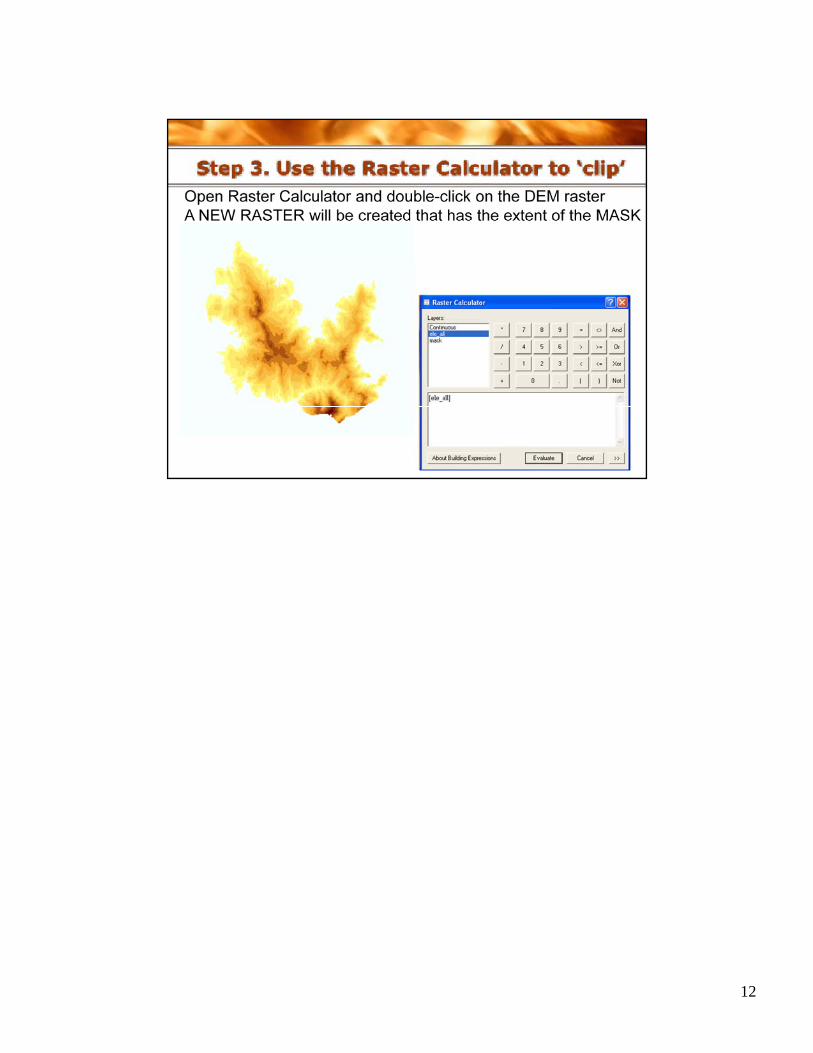
12

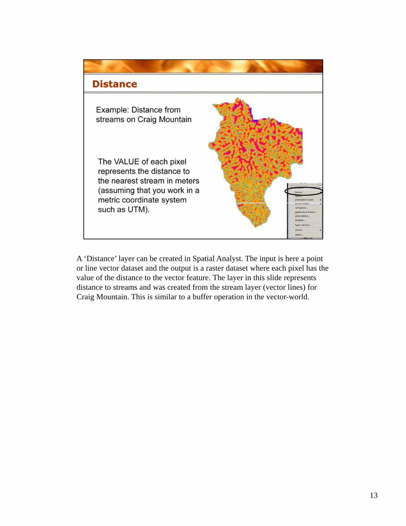
A ‘Distance’ layer can be created in Spatial Analyst. The input is here a point or line vector dataset and the output is a raster dataset where each pixel has the value of the distance to the vector feature. The layer in this slide represents distance to streams and was created from the stream layer (vector lines) for Craig Mountain. This is similar to a buffer operation in the vector-world.

13

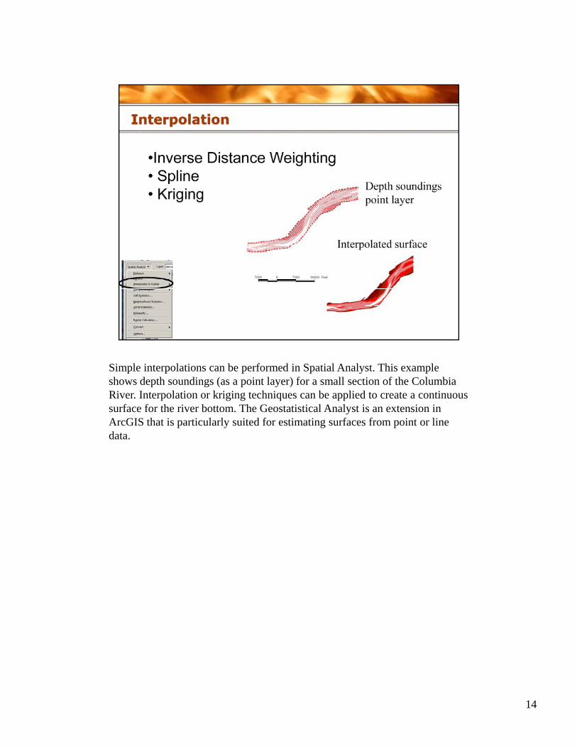
Simple interpolations can be performed in Spatial Analyst. This example shows depth soundings (as a point layer) for a small section of the Columbia River. Interpolation or kriging techniques can be applied to create a continuous surface for the river bottom. The Geostatistical Analyst is an extension in ArcGIS that is particularly suited for estimating surfaces from point or line data.

14

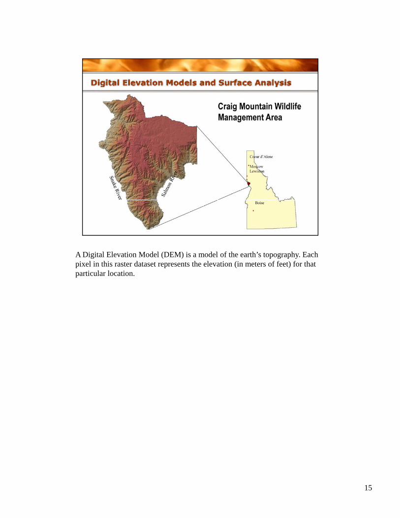
A Digital Elevation Model (DEM) is a model of the earth’s topography. Each pixel in this raster dataset represents the elevation (in meters of feet) for that particular location.

15

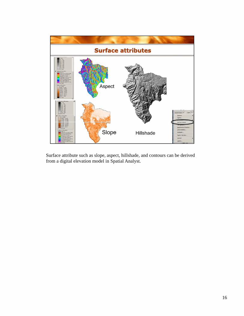
Surface attribute such as slope, aspect, hillshade, and contours can be derived from a digital elevation model in Spatial Analyst.

16

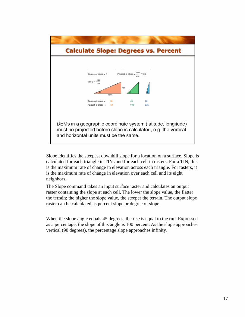
Slope identifies the steepest downhill slope for a location on a surface. Slope is calculated for each triangle in TINs and for each cell in rasters. For a TIN, this is the maximum rate of change in elevation across each triangle. For rasters, it is the maximum rate of change in elevation over each cell and its eight neighbors. The Slope command takes an input surface raster and calculates an output raster containing the slope at each cell. The lower the slope value, the flatter g p pthe terrain; the higher the slope value, the steeper the terrain. The output slope raster can be calculated as percent slope or degree of slope.

When the slope angle equals 45 degrees, the rise is equal to the run. Expressed as a percentage, the slope of this angle is 100 percent. As the slope approaches vertical (90 degrees) the percentage slope approaches infinityvertical (90 degrees), the percentage slope approaches infinity.

17

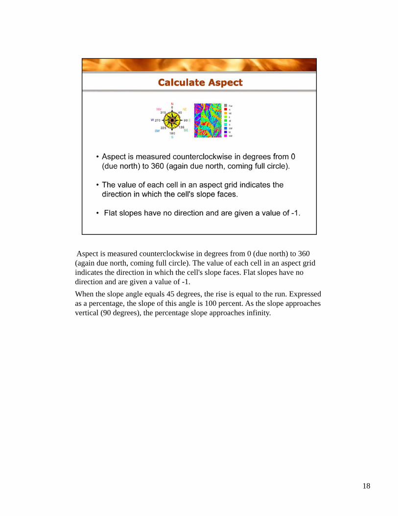
Aspect is measured counterclockwise in degrees from 0 (due north) to 360 (again due north, coming full circle). The value of each cell in an aspect grid indicates the direction in which the cell's slope faces. Flat slopes have no direction and are given a value of -1.When the slope angle equals 45 degrees, the rise is equal to the run. Expressed as a percentage, the slope of this angle is 100 percent. As the slope approaches vertical (90 degrees), the percentage slope approaches infinity.( g ) p g p pp y

18

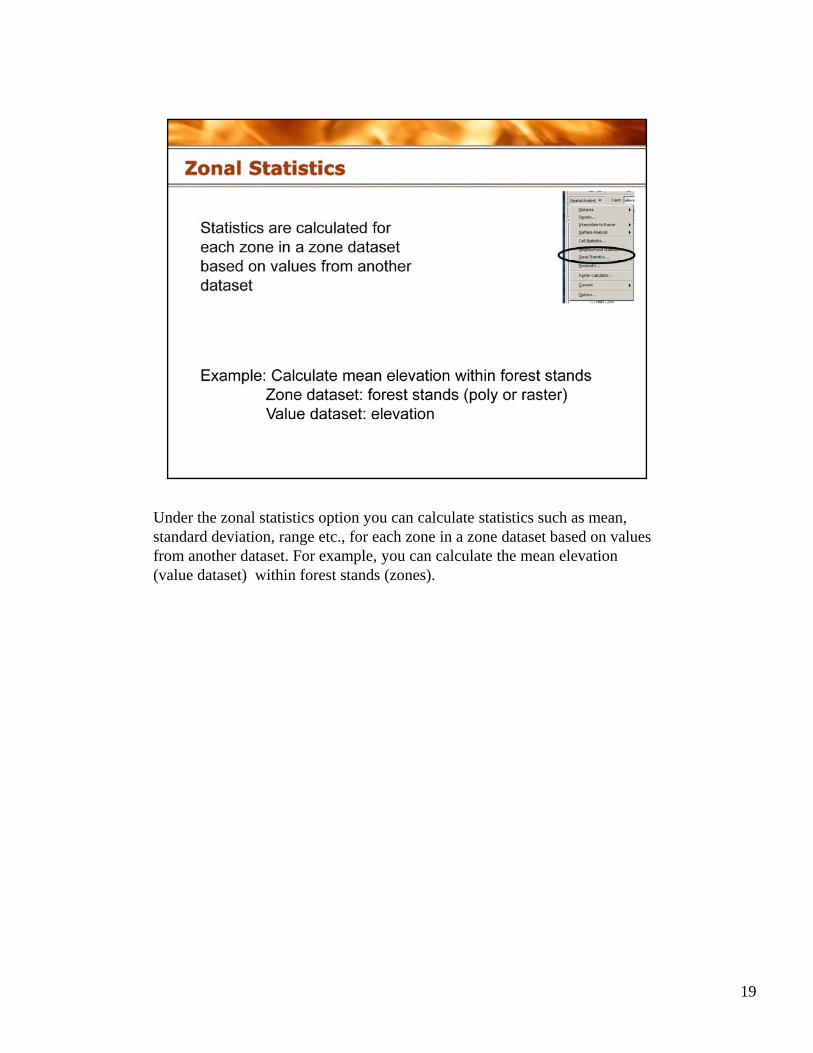
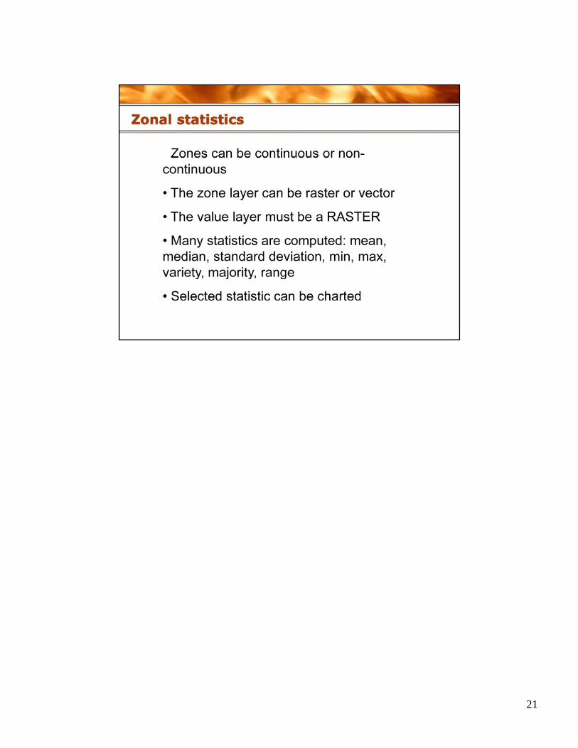
Under the zonal statistics option you can calculate statistics such as mean, standard deviation, range etc., for each zone in a zone dataset based on values from another dataset. For example, you can calculate the mean elevation (value dataset) within forest stands (zones).

19

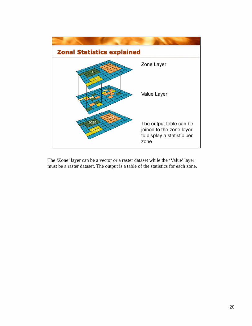
The ‘Zone’ layer can be a vector or a raster dataset while the ‘Value’ layer must be a raster dataset. The output is a table of the statistics for each zone.

20

21

22

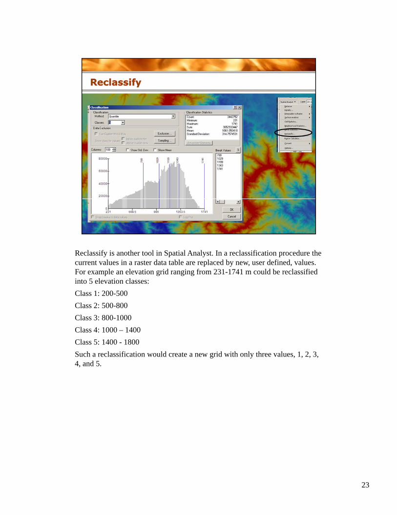
Reclassify is another tool in Spatial Analyst. In a reclassification procedure the current values in a raster data table are replaced by new, user defined, values. For example an elevation grid ranging from 231-1741 m could be reclassified into 5 elevation classes:Class 1: 200-500Class 2: 500-800Cl 3 800 1000Class 3: 800-1000Class 4: 1000 – 1400Class 5: 1400 - 1800Such a reclassification would create a new grid with only three values, 1, 2, 3, 4, and 5.

23

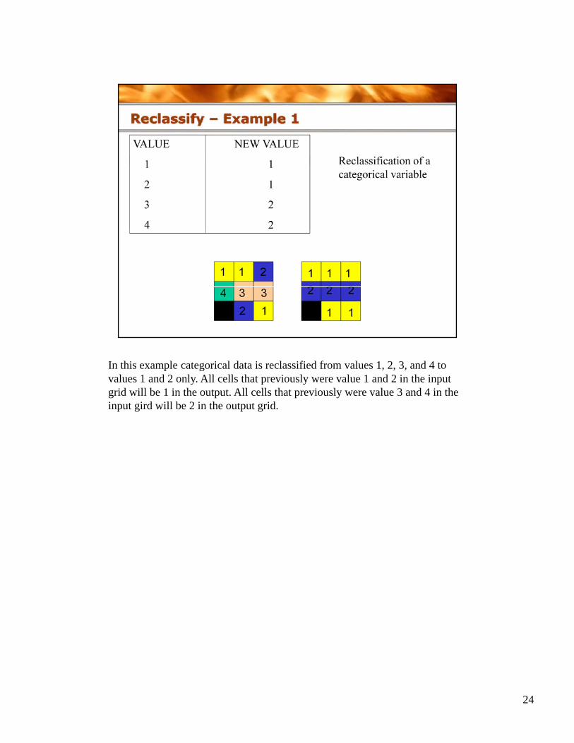
In this example categorical data is reclassified from values 1, 2, 3, and 4 to values 1 and 2 only. All cells that previously were value 1 and 2 in the input grid will be 1 in the output. All cells that previously were value 3 and 4 in the input gird will be 2 in the output grid.

24

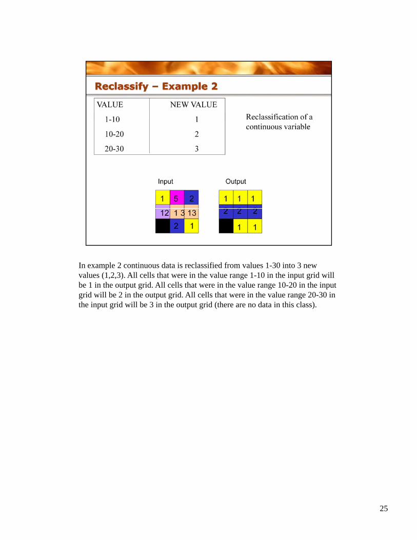
In example 2 continuous data is reclassified from values 1-30 into 3 new values (1,2,3). All cells that were in the value range 1-10 in the input grid will be 1 in the output grid. All cells that were in the value range 10-20 in the input grid will be 2 in the output grid. All cells that were in the value range 20-30 in the input grid will be 3 in the output grid (there are no data in this class).

25

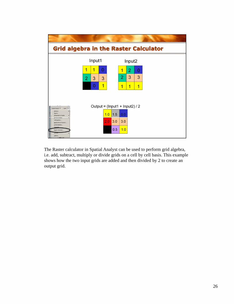
The Raster calculator in Spatial Analyst can be used to perform grid algebra, i.e. add, subtract, multiply or divide grids on a cell by cell basis. This example shows how the two input grids are added and then divided by 2 to create an output grid.

26

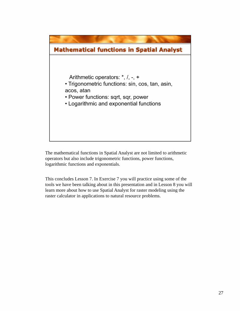
The mathematical functions in Spatial Analyst are not limited to arithmetic operators but also include trigonometric functions, power functions, logarithmic functions and exponentials.

This concludes Lesson 7. In Exercise 7 you will practice using some of the tools we have been talking about in this presentation and in Lesson 8 you will learn more about how to use Spatial Analyst for raster modeling using thelearn more about how to use Spatial Analyst for raster modeling using the raster calculator in applications to natural resource problems.

27

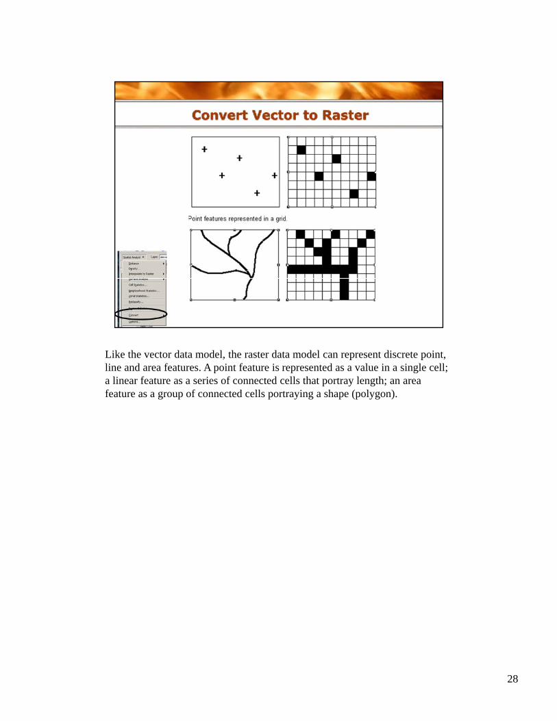
Like the vector data model, the raster data model can represent discrete point, line and area features. A point feature is represented as a value in a single cell; a linear feature as a series of connected cells that portray length; an area feature as a group of connected cells portraying a shape (polygon).

28

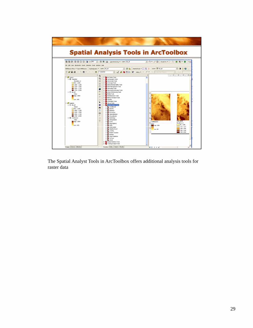
The Spatial Analyst Tools in ArcToolbox offers additional analysis tools for raster data

29

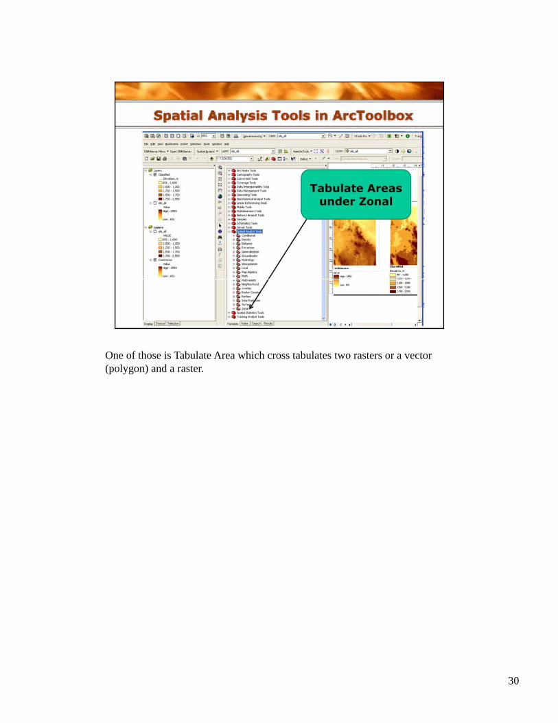
One of those is Tabulate Area which cross tabulates two rasters or a vector (polygon) and a raster.

30

31

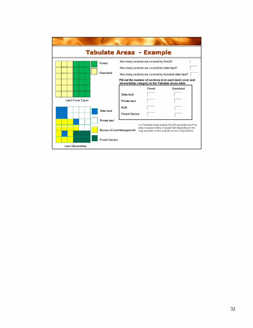
32

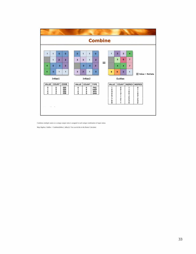
Combines multiple rasters so a unique output value is assigned to each unique combination of input values.

M Al b O tR C bi (I R 1 I R 2) Y d thi i th R t C l l tMap Algebra: OutRas = Combine(InRas1, InRas2). You can do this in the Raster Calculator

33