Spatial Point Patterns & Complete Spatial RandomnessGeog 210C

Introduction to Spatial Data Analysis

Chris Funk

Lecture 6

Where are we? WEEK DATE TITLE

1 Mar 29Mar 31

Overview of Statistical Analysis of Spatial Data(.pdf)Univariate Sample Statistics(.pdf)

2 Apr 05Apr 07

Univariate Random Variables(.pdf)Intensity Analysis of Spatial Point Patterns(.pdf)

3Apr 12Apr 14

Interaction Analysis of Spatial Point Patterns (.pdf)Point Patterns & Complete Spatial Randomness

4 Apr 19Apr 21

Descriptive Statistics (Bivariate & Multivariate)Empirical Semivariograms

5Apr 26Apr 28

Elements of Spatial Stochastic Processes IModeling Health Outcomes

6May 03May 05

Elements of Spatial Stochastic Processes IIModeling Semivariograms

7May 10May 12

Spatial Interpolation ExampleSimple Kriging

8May 17May 19

Not So Simple KrigingExplaining Covariance

9May 24May 26

Principal Component Analysis-IPrincipal Component Analysis-II

10June 01June 03

Sampling DesignDeterministic + Stochastic Model Combinations

2

3

Forward/Inverse Statistical Problems

Schrodinger’s Box

Forward problem

Inverse Problem

Data Generatingprocess

Data/Map

A point pattern … process? random?

C. Funk Geog 210C Spring 20104

Topography as exogenous variable?

5

Slope, Elevation, 1/Compound Topographic IndexMapped as Red/Green/Blue

C. Funk Geog 210C Spring 20106

Outline

Concepts & NotationCompletely Random Spatial Point Process ModelsDeriving Sampling Distributions Under CSR via Monte Carlo SimulationDeriving Sampling Distributions Under CSR AnalyticallyBeyond CSR Point Process ModelsPoints To Remember

7

Stages in The Analysis of Spatial Point Patterns

Descriptive analysisquantitative & graphical tools for characterizing spatial point patterns; different tools are appropriate for investigating intensity and interaction effects, e.g., kernel density estimation versus Ghatfunctioninformation on whether events are clustered or evenly distributed in space

Limitationsno assessment of how much clustered or how much evenly-spaced is an observed point patternno yardstick against which to compare observed values (or graph) of computed statistics, e.g., Ghat function

Confirmatory analysisAssessment of whether an observed spatial point pattern can be regarded as one (out of many) realization from a particular spatial point processMeasures of confidence or likelihood with which the above assessment can be made

8

Some Terminology

Null process or hypothesisSpatial process hypothesized to be the generating mechanism of spatial patternsIn this lecture, we'll focus on the null hypothesis of complete spatial randomness (CSR)

SamplesRealizations (outcomes) from a hypothesized process, e.g., set of alternative point patterns generated from the null

process of CSR

Sampling distribution of a statisticsample statistic = a summary measure, e.g., mean or entire CDF, characterizing (and thus computed from) a samplesampling distribution of a statistic = distribution, e.g., histogram, of such a summary measure computed from many alternative samples generated from the null process

C. Funk Geog 210C Spring 20109

Some Notation

Point eventsSet of n locations of events occurring in a study area:

Variable of interesty(s) = number of events (a count) within arbitrary domain or support s with measure (length, area, volume) |s|; support s is centered at an arbitrary location u and can also be denoted as s(u). In statistics, y(s) is regarded a realization of a random variable (RV) Y(s), and there can be many such realizations {ys(l); l = 1…L}; their frequency of occurrence is dictated by the PDF

Random processA collection of RVs, one per support, is termed a random process. In general, such RVs can jointly attain outcomes at different supports; the joint frequency of occurrence of such realizations is dictated by the multivariate PDF of these RVs

coordinate vector of i-th event location

study domain, a subset of a K-dimensional space RK

belongs to

10

Realizations from A Random Process

l=1

l=…

l=L

ScaleMatters!

11

Expectation of Random Variables & Local Intensity

Long-term average (“climatology") of any RV Y(s), typically denoted as: µY(s) = E{Y(s)}

for count RVs, we often use the notation λ(s) instead of Y(s). The argument (s) in E{Y(s)} emphasizes that the expectation of RV Y(s) is specific to support s, and could be different than the expectation E{Y(s’)} at support s’

Local intensity λ(u)Mean number of events per unit area at an arbitrary location or point u, formally defined as:

λ(u) is thought to belong to an intensity “surface"

12

Recap

Confirmatory analysis of spatial point patternsAllows us to quantify the departure of results obtained via exploratory tools, e.g average dmin or G(d), from expected results derived under a specific null hypotheses (here CSR)Can be used to assess to what extent observed point patterns can be regarded as realizations from a particular spatial process (here CSR)CSR involves: i) a constant intensity and (ii) no event-to-event

interaction

Sampling distribution of a test statisticLies at the heart of any statistical hypothesis testing procedure, and is tied to a particular null hypothesis (and a particular study domain)Simulation and analytical derivations are two alternative ways of computing such sampling distributions (the latter being increasingly replaced by the former)Watch out for edge effects when using analytically derived

sampling distributions …

13

Complete Spatial Randomness (CSR)

Loose definitionSpatial process, here a spatial point process, serving as a generating mechanism of spatial point patterns, with the following characteristics: intensity λ (mean # of events per unit area) is constant in any

subregion s of the study domain D ⇒ no environmental or first-order effects

Position or occurrence of any event is independent of occurrence of any other event ⇒ no event-to-event interaction or second-order effects

Two versions of CSR point process modelsBinomial point process: there are n events in study domain D, which are located at random Poisson point process: the number of events n is a realization from a Poisson distribution; once a realization nl of n is generated, these nl points are located at random within D

For a Poisson point process, number of events n in study region D varies from realization to realization, whereas this number is fixed for a Binomial point process. In other words, if we generate L sets of simulated point patterns from a Poisson point process, there will be L different numbers of events over the L realizations; for the Binomial process, these L numbers will all be the same .

14

Homogeneous Poisson Point Process

Formal definitionNumber of events y≡y(s), a count, within an arbitrary subregion s with area |s| is a realization of a random variable Y≡Y(s) with a Poisson PDF:

Any two RVs Y(s) and Y(s’) defined over two non-overlapping subregions s and s’ are independent

15

Homogeneous Poisson Point Process: Simulation (I)

SettingConsider a study region D of size |D| = 100x100 and an overall intensity λ= 0.01, leading to an expected count of E{Y(D)} = |D| = 100 events within D. Let D be partitioned into Q = 25 square quadrats of equal size |sq|= 20x20, for all q. One can now define a set of Q = 25 random variables {Y(sq), q = 1…Q}, one per quadrat. Under CSR, the RV Y(s) associated with any quadrat has an expected count of E{Y(s)} = |s| = 4 events (per 1st-order stationarity), and counts across different quadrats are independent

ObjectiveGenerate a realization (a point pattern) from a homogeneous Poisson process; in other words, simulate counts from the Q = 25 RVs {Y(sq); q = 1…Q}. Once a count y(s) is simulated for quadrat s, y(s) events (points) are placed at random within s. Since E{Y(s)} = 4, we need to generate, on average, 4 events within any quadrat s. Since counts across quadrats are independent, simulated events within s do not influence the generation of events outside s. All this amount to zooming in to a particular quadrat s, generating a count y(s) from a Poisson distribution with mean E{Y(s)} = 4, and then repeating for all Q quadrats. This is the same as generating, on average, 100 events randomly within D from a RV Y(D) with a Poisson distribution with mean E{Y(D)} = |D| = 100; then, y(D) would denote a simulated count over D

16

Homogeneous Poisson Point Process: Flowchart (II)

Let L be the number of realizations (alternative point patterns) to generate, and nl be the number of events of the (to be) simulated point pattern in the l-th realization (using the previous notation, nl ≡ y(D))

1. generate L numbers (counts) {nl ; l = 1… L} from a Poisson distribution with mean (λ |D| = expected # of events); these Lcounts serve as numbers of events for the point patterns to be simulated

2. for the l-th realization, simulate the locations of nl events in D, by generating nl values of x- and y-coordinates, independent and uniformly distributed along the two sides of a rectangle enclosing D

3. reject any events that do not lie in D, and repeat step 2 until nlevents are obtained within D; steps 1 & 2 constitute a realization from a Binomial process with nl events

4. repeat steps 2 and 3 with another # of events nl‘, to generate another realization, i.e., the l’-th simulated point pattern

17

Realizations from a Binomial Point Process

Two realizations from a Binomial spatial point process with n = 50 events:

Events can appear clustered, but this is due to chanceif 1st-order effects were present, i.e., if λ varied through the study region, more events should appear at same places from one realization to another; hence, clusters would be formed around high intensity areas in each realization, even if no interaction was included in the modelif strong 2nd-order effects were present, events would appear clustered in every realization; such clusters, however, would appear in different places from one realization to another if no 1st-order effects were present

18

Sampling Distribution of a Statistic Under CSR (I)

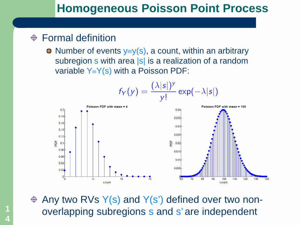
Sample statisticMean event-to-nearest-event (E2NE) distance; here the variable of interest is the distance (E2NE) between any event an its nearest neighbor event, and the selected summary statistic is the mean of those distances:

Constructing sampling distribution of mean E2NE via simulation1. Adopt a null hypothesis, here CSR, as a mechanism for generating

point patterns; that null hypothesis also includes the parameters, here λ, of the population

2. Generate (simulate) one realization of a point pattern under CSR3. Compute simulated average dmin value from that realization4. Rrepeat steps (1) and (2), say, L = 1000 times to obtain L

simulated average dmin values5. Histogram of L simulated average dmin values = sampling

distribution of mean E2NE distance under the null hypothesis

19

Sampling Distribution of a Statistic Under CSR (II)

Two realizations of a Binomial point process with n = 50 events:

Sampling distribution or histogram of average dmin values from 500 simulated (under CSR) point patterns, each having n = 50 events

20

Sampling Distribution of a Statistic Under CSR (III)

Two realizations of a Binomial point process with n = 100 events:

Sampling distribution or histogram of average dmin values from 500 simulated (under CSR) point patterns, each having n = 100 events

21

Looking at Observed Point Patterns (I)

Sampling distributionof average dmin values under CSR

Two observed point patterns with n = 100 events:

Question: Could these two point patterns be realizations under CSR?

Answer: No, and this can be said with “great” confidence; pattern on left (right) has “much” larger (smaller) mean E2NE distance than “expected” under CSR

22

Looking at Observed Point Patterns (II)

Observed point pattern with n = 100 events, and sampling distribution of average dmin under CSR:

Question: Is observed point pattern “more clustered: than a CSR-generated one?

Answer: “Most probably” no, since observed average dmin = 5.18 (black vertical bar) lies at the center of the sampling distribution of average dminvalues under CSR

23

Looking at Observed Point Patterns (III)

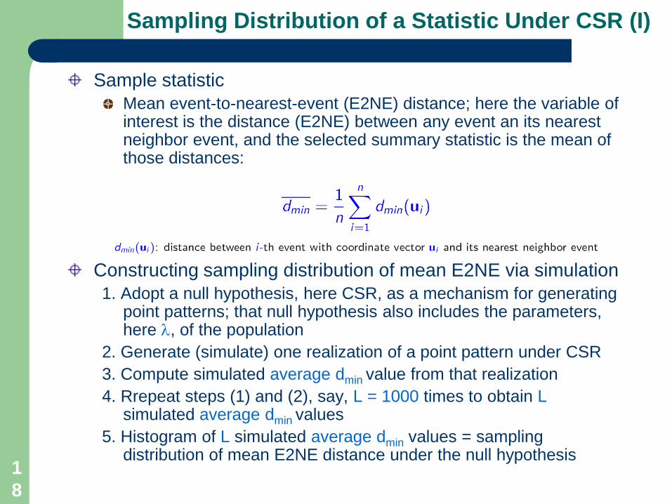
Observed point pattern with n = 100 events, and sampling distribution of dmin under CSR:

Question: Is this pattern more clustered than a CSR-generated one?Equivalent question: Since small average dmin values indicate clustering, what is the observed area to the left of average dmin on the sampling distribution under CSR?Answer: The area under the curve of the sampling distribution to the left of observed average dmin = 4.65 is an indication of how unlikely is the observed pattern to be generated by CSR: the smaller that area, the more unlike is the pattern to be a realization under CSR.

NOTE: if we were asking whether the observed point pattern was more even (less clustered) than a CSR-generated one, we would be looking at the area under the curve to the right of 4.65, since we would be interested in larger (than CSR-related) such distance values

24

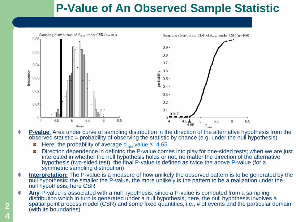
P-Value of An Observed Sample Statistic

P-value: Area under curve of sampling distribution in the direction of the alternative hypothesis from the observed statistic = probability of observing the statistic by chance (e.g. under the null hypothesis).

Here, the probability of average dmin value ≤ 4.65Direction dependence in defining the P-value comes into play for one-sided tests; when we are just interested in whether the null hypothesis holds or not, no matter the direction of the alternative hypothesis (two-sided test), the final P-value is defined as twice the above P-value (for a symmetric sampling distribution)

Interpretation: The P-value is a measure of how unlikely the observed pattern is to be generated by the null hypothesis: the smaller the P-value, the more unlikely is the pattern to be a realization under the null hypothesis, here CSRAny P-value is associated with a null hypothesis, since a P-value is computed from a sampling distribution which in turn is generated under a null hypothesis; here, the null hypothesis involves a spatial point process model (CSR) and some fixed quantities, i.e., # of events and the particular domain (with its boundaries)

25

Sampling Distribution of G Function Under CSR

Interpretation: Plots provide envelope of simulated minimum and maximum G(d)curves under the null hypothesis of CSR, for a given overall intensity computed as n/|D|,hence tied to the # of events considered and the particular domain; The larger n is (more events in the domain), the tighter that envelope.

Link to hypothesis testing: To assess whether an observed point pattern can be regarded a realization from a CSR null process, evaluate the relative position (within that envelope) of the observed G(d) curve

26

Testing Observed Ghat Plots Against CSR (I)

Two observed point patterns with n = 100 events:

Question: Could these two point patterns be realizations under CSR?

“Most probably” no, since the observed G(d) curve lies outside the simulation envelope

27

Testing Observed Ghat Plots Against CSR (II)

Observed point pattern with n = 100 events:

Question: Could this point pattern be a realization under CSR?

Answer: Most probably yes, since observed G(d) curve lies very close to mean simulated plot, and is well within the simulation envelope

28

Analytically-Derived Sampling Distributions

ConceptFor simple domains, e.g., rectangles, there exist mathematical formulae that provide the expected values of sample statistics under CSR; in other words, people have already calculated what is the mean of a very large number of simulated average dmin or G(d) values under CSR, without ever touching a computerThese formulae have been derived before the advent of powerful computers, and have been used for a long time in point pattern analysissince, no simulation runs are involved, such analytically-derived formulae can be easily used without resorting to computer-intensive simulation procedures

LimitationsAnalytically-derived formulae need to account for the fact that events near the boundary of the study region do not have the same number of neighbors as events in the middle of that regionSuch edge effects can be taken care of when the study region has simple geometry, e.g., for rectangles

DefinitionAverage of all N E2NE values

Note that a single number does not suffice to a describe point pattern

Checking for CSR1. Compute expected value of mean nearest-neighbor distance, under

CSR:

2. Form ratio R:

Interpretation: R < 1 → observed nearest neighbor distances shorter than expected →

tendency towards clustering R > 1 → tendency towards evenly spaced events

29

CSR-Expected Mean Nearest Neighbor Distance

Result depends heavily upon study area definition (used to compute λ)

30

CSR-Expected G and F Functions

G function definition: Proportion of event-to-nearest-event distances dmin(ui) no greater than given distance cutoff d

→ cumulative distribution function (CDF) of all n event-to-nearest-event distances:

F function definition: Proportion of point-to-nearest- event distances dmin(tp) no greater than given distance cutoff d

→ CDF of all m point-to-nearest-event distances:

Expected G and F function under CSR for relatively small distances to avoid edge effects:

Checking for CSR: compare empirical functions G(d) and F(d) with their theoretical counterparts E{G(d)} and E{F(d)} under CSR

31

Examples of Observed and CSR-Expected G Functions

0

0.2

0.4

0.6

0.8

1

1.2

0 50 100

CD

F

Event-to-nearest-neighbor-event distance

Exp(G) unde CSR

*****

32

Examples of Observed and CSR-Expected F Functions

33

Example with Evenly Spaced Events

34

The K Function

1. construct set of concentric circles (of increasing radius d) around each event

2. compute # of events in each distance “band”, excluding event at the center

3. cumulative number of events up to radius daround all events becomes the sample Kfunction K(d)

35

CSR-Expected K Function

K(d) & L(d) functions under CSR

this can become a very large number (due to d2), and consequently small differences between K(d) and E{K(d)}cannot be easily resolveduse L function instead:

With E{L(d)} = 0Interpreting the L function

L(d) > 0 implies clusteringL(d) < 0 implies stratificationWatch out for edge effectsReality tends to be ‘patchy’Can we use Monte Carlo simulations instead of edge

effect corrections?

36

Examples of L Functions

L(d) > 0 → more events are separated by distance d than expected under CSR → clustering

37

Other Spatial Point Process Models

Heterogeneous with no second-order effectsHeterogeneous Poisson process: intensity is made spatially varying λ(u), and could be linked to covariates. Simulation proceeds by generating events from a homogeneous Poisson process with intensity λmax = max{λ(u)}, and then independently keeping an event at u with probability λ(u)/λmax

Cox process: spatially varying intensity λ(u) in a non-deterministic way (doubly stochastic process); a field of λ(u)-values is first simulated, and then

simulation proceeds as in the heterogeneous Poisson modelHomogeneous with second-order effects

Poisson cluster process: i) Simulate centroids of “parent” events from a homogeneous Poisson processii) Associate a simulated number of “off-spring” with each parent centroidiii) Simulate the locations of off-spring around each parent centroid according to

some bivariate PDF, and iv) Keep only the locations of off-sprind as the final simulated point pattern

There also exist processes with both first- and second-order effectse.g., the inhomogeneous Poisson cluster process : : :

38

Recap (I)

Confirmatory analysis of spatial point patternsAllows us to quantify the departure of results obtained via exploratory tools, e.g average dmin or G(d), from expected results derived under a specific null hypotheses (here CSR)Can be used to assess to what extent observed point patterns can be regarded as realizations from a particular spatial process (here CSR)CSR involves: i) a constant intensity and (ii) no event-to-event

interaction

Sampling distribution of a test statisticLies at the heart of any statistical hypothesis testing procedure, and is tied to a particular null hypothesis (and a particular study domain)Simulation and analytical derivations are two alternative ways of computing such sampling distributions (the latter being increasingly replaced by the former)Watch out for edge effects when using analytically derived

sampling distributions …

39

Recap (II)

More interesting spatial point process modelsHeterogeneous Poisson process, Cox process, Poisson cluster process …Note: It is almost impossible to assess whether an observed point pattern (a single realization from a hypothesized point process) stems from a process with only first- or only second-order effects or a combination thereof; different processes could yield indistinguishable realizations under certain parameter combinations (equi-finality)

Parameter estimation?In practice, we are most often dealing with the problem of estimating the parameters of a spatial point process model from data, i.e., from an observed spatial point pattern. This is an inverse problem, as opposed to the forward problem of generating patterns from processes. The inverse problem, however, is under-determined, mostly because we only have 1realization (the observed pattern) from a hypothesized process

Schrodinger’s Box

Forward problem

Inverse Problem

Data Generatingprocess

Data/Map