Spectral Line BroadeningHubeny & Mihalas Chap. 8

Gray Chap. 11

Natural Broadening Doppler Broadening

Collisional Broadening: Impact, Statistical, Quantum Theories

1

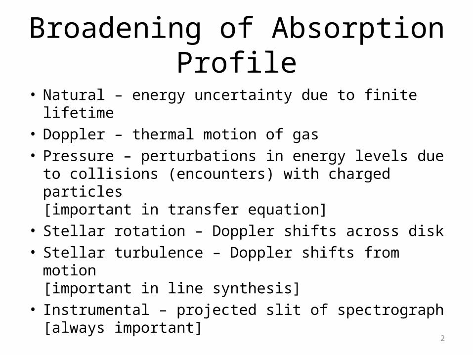
Broadening of Absorption Profile

• Natural – energy uncertainty due to finite lifetime• Doppler – thermal motion of gas• Pressure – perturbations in energy levels due to

collisions (encounters) with charged particles[important in transfer equation]

• Stellar rotation – Doppler shifts across disk• Stellar turbulence – Doppler shifts from motion

[important in line synthesis]• Instrumental – projected slit of spectrograph

[always important]2

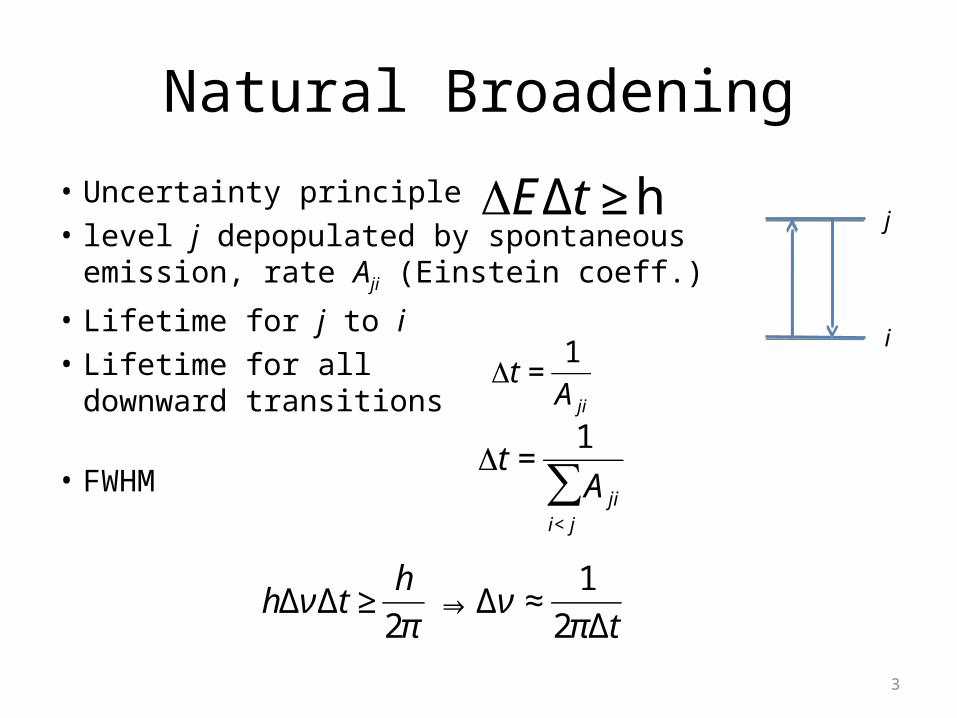
Natural Broadening

• Uncertainty principle • level j depopulated by spontaneous emission,

rate Aji (Einstein coeff.)

• Lifetime for j to i • Lifetime for all

downward transitions

• FWHM

3

€

ΔEΔt ≥ h

€

Δt =1

A ji

€

Δt =1

A jii< j

∑

€

hΔνΔt ≥h

2π⇒ Δν ≈

1

2πΔt

j

i

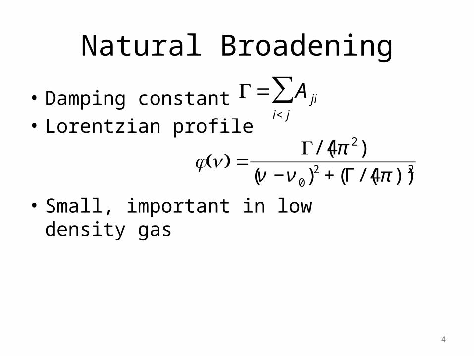
Natural Broadening

• Damping constant • Lorentzian profile

• Small, important in low density gas

4

€

Γ= A jii< j

∑

€

φ ν( ) =Γ/(4π 2)

(ν −ν 0)2 + (Γ/(4π ))2

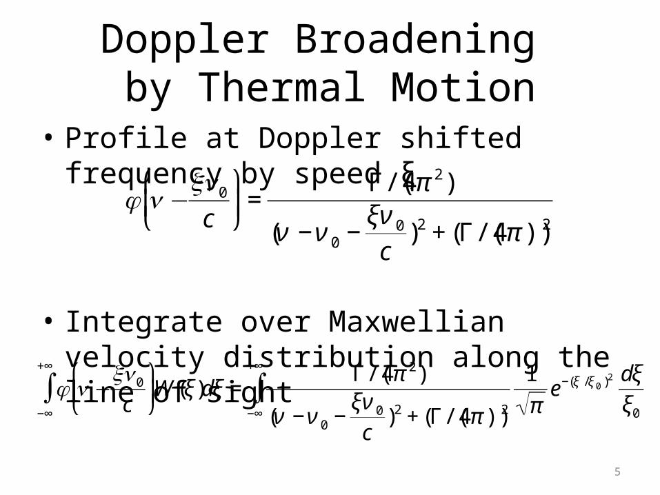
Doppler Broadening by Thermal Motion

• Profile at Doppler shifted frequency by speed ξ

• Integrate over Maxwellian velocity distribution along the line of sight

5

€

φ ν −ξν 0

c

⎛

⎝ ⎜

⎞

⎠ ⎟=

Γ/(4π 2)

(ν −ν 0 −ξν 0

c)2 + (Γ/(4π ))2

€

φ ν −ξν 0

c

⎛

⎝ ⎜

⎞

⎠ ⎟W (ξ)

−∞

+∞

∫ dξ =Γ/(4π 2)

(ν −ν 0 −ξν 0

c)2 + (Γ/(4π ))2−∞

+∞

∫ 1

πe−(ξ /ξ 0 )2 dξ

ξ0

Doppler Broadening by Thermal Motion

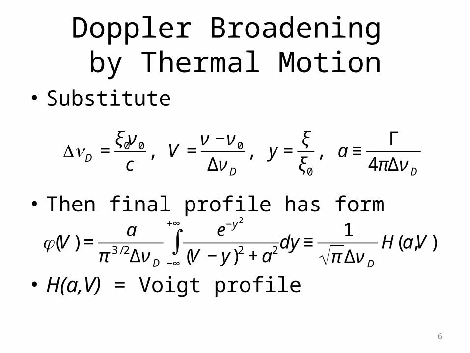
• Substitute

• Then final profile has form

• H(a,V) = Voigt profile

6

€

ΔνD =ξ0ν 0

c, V =

ν −ν 0

Δν D

, y =ξ

ξ0

, a ≡Γ

4πΔν D

€

φ(V ) =a

π 3 / 2Δν D

e−y 2

(V − y)2 + a2−∞

+∞

∫ dy ≡1

π Δν D

H(a,V )

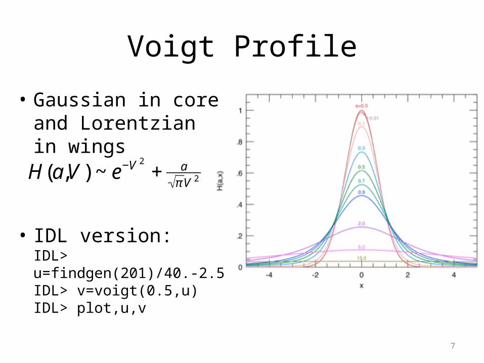
Voigt Profile

• Gaussian in core and Lorentzian in wings

• IDL version:IDL> u=findgen(201)/40.-2.5IDL> v=voigt(0.5,u)IDL> plot,u,v

7

€

H(a,V ) ~ e−V 2

+ aπV 2

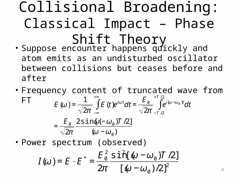
Collisional Broadening:Classical Impact – Phase Shift Theory

• Suppose encounter happens quickly and atom emits as an undisturbed oscillator between collisions but ceases before and after

• Frequency content of truncated wave from FT

• Power spectrum (observed)

8€

E(ω) =1

2πE(t)e iω tdt =

E0

2π−∞

+∞

∫ e i(ω −ω 0 )t

−T / 2

+T / 2

∫ dt

=E0

2π

2sin[(ω −ω0)T /2]

(ω −ω0)

€

I(ω) = E⋅ E * =E0

2

2π

sin2[(ω −ω0)T /2]

[(ω −ω0) /2]2

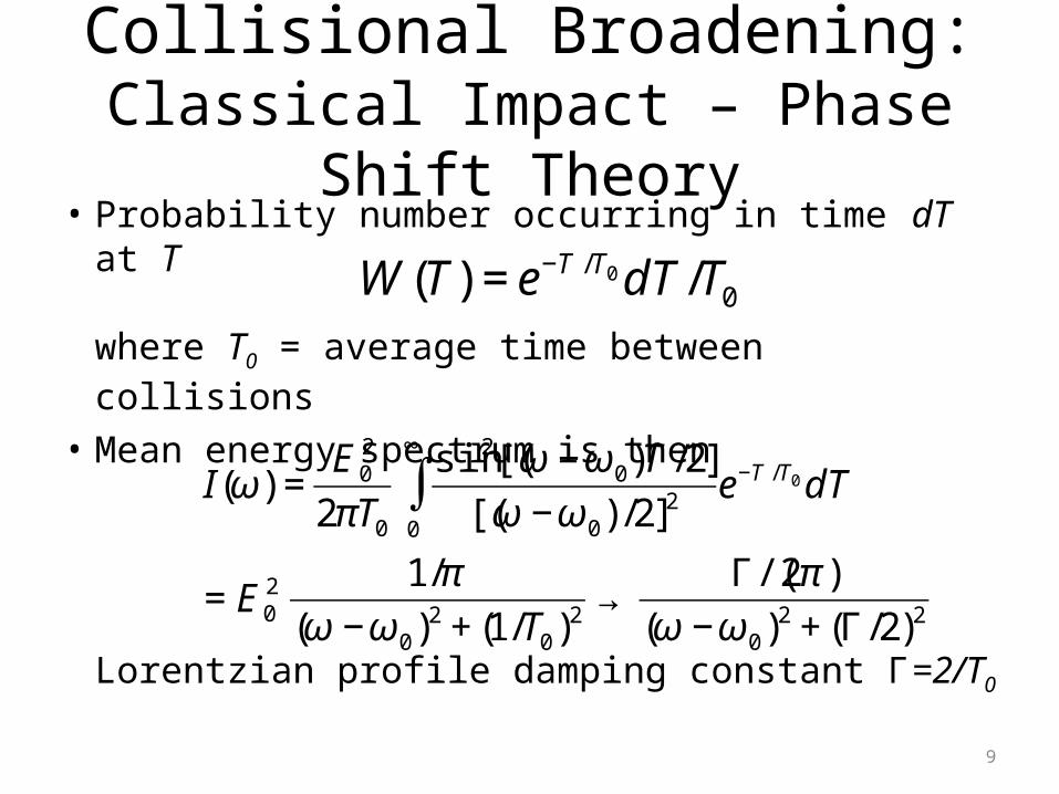
Collisional Broadening:Classical Impact – Phase Shift Theory

• Probability number occurring in time dT at T

where T0 = average time between collisions

• Mean energy spectrum is then

Lorentzian profile damping constant Γ=2/T0

9

€

W (T) = e−T /T0dT /T0

€

I(ω) =E0

2

2πT0

sin2[(ω −ω0)T /2]

[(ω −ω0) /2]20

∞

∫ e−T /T0dT

= E02 1/π

(ω −ω0)2 + (1/T0)2 →Γ/(2π )

(ω −ω0)2 + (Γ/2)2

Collisional Broadening:Classical Impact – Phase Shift Theory

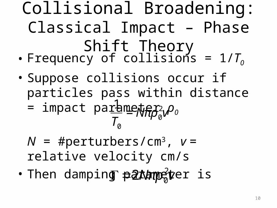
• Frequency of collisions = 1/T0

• Suppose collisions occur if particles pass within distance = impact parameter ρ0

N = #perturbers/cm3, v = relative velocity cm/s• Then damping parameter is

10

€

1

T0

= Nπρ 02v

€

Γ=2Nπρ 02v

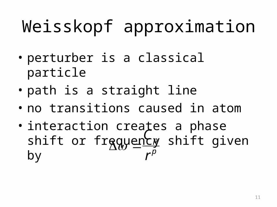
Weisskopf approximation

• perturber is a classical particle• path is a straight line• no transitions caused in atom• interaction creates a phase shift or frequency

shift given by

11

€

Δω =Cp

r p

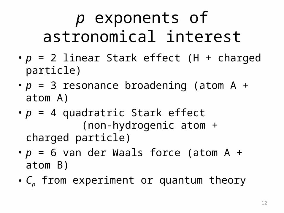
p exponents of astronomical interest

• p = 2 linear Stark effect (H + charged particle)• p = 3 resonance broadening (atom A + atom

A)• p = 4 quadratric Stark effect

(non-hydrogenic atom + charged particle)• p = 6 van der Waals force (atom A + atom B)• Cp from experiment or quantum theory

12

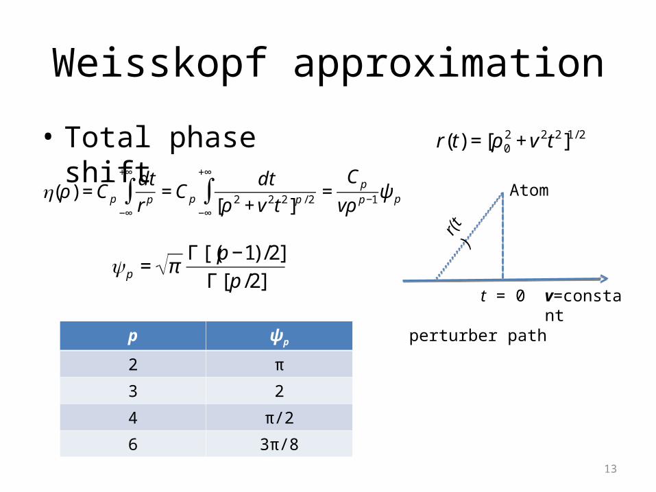
Weisskopf approximation

€

r(t) = [ρ 02 + v 2t 2]1/ 2

13

Atom

perturber path

t = 0 v=constant

r(t)

• Total phase shift

€

η(ρ) =Cp

dt

r p =−∞

+∞

∫ Cp

dt

[ρ 2 + v 2t 2]p / 2 =−∞

+∞

∫Cp

vρ p−1ψ p

€

ψ p = πΓ [(p −1) /2]

Γ [p /2]

p ψp

2 π

3 2

4 π/2

6 3π/8

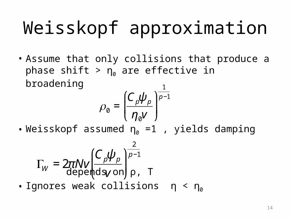
Weisskopf approximation

• Assume that only collisions that produce a phase shift > η0 are effective in broadening

• Weisskopf assumed η0 =1 , yields damping

depends on ρ, T • Ignores weak collisions η < η0

14

€

ρ0 =Cpψ p

η0v

⎛

⎝ ⎜

⎞

⎠ ⎟

1

p−1

€

ΓW = 2πNvCpψ p

v

⎛

⎝ ⎜

⎞

⎠ ⎟

2

p−1

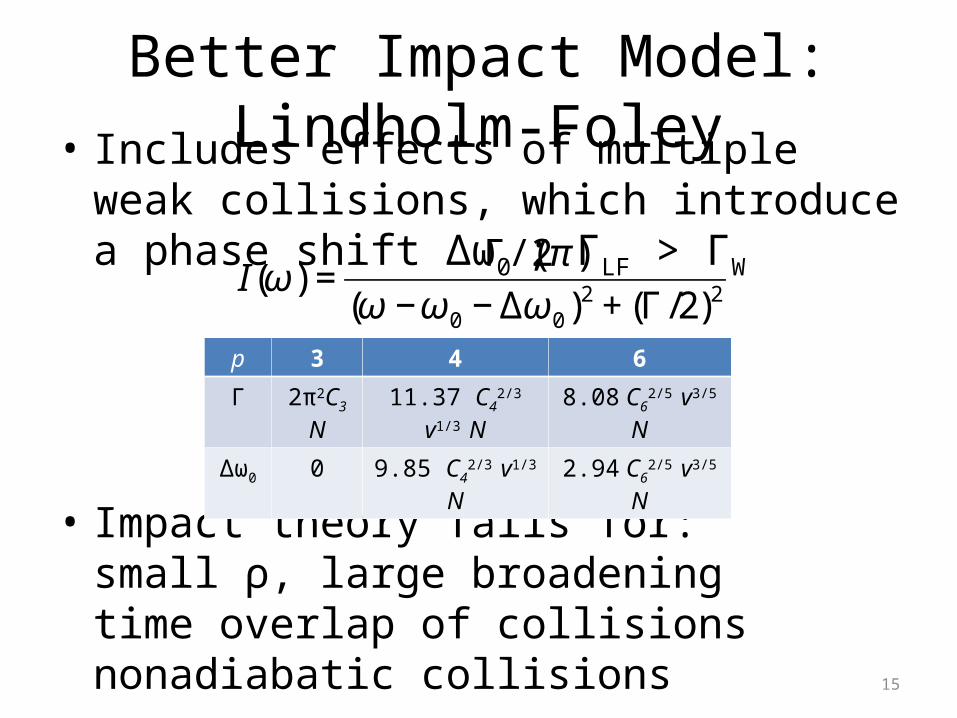
Better Impact Model: Lindholm-Foley• Includes effects of multiple weak collisions,

which introduce a phase shift Δω0 ; ΓLF > ΓW

• Impact theory fails for: small ρ, large broadeningtime overlap of collisionsnonadiabatic collisions

15

€

I(ω) =Γ/(2π )

(ω −ω0 − Δω0)2 + (Γ/2)2

p 3 4 6

Γ 2π2C3N 11.37 C42/3 v1/3 N 8.08 C6

2/5 v3/5 N

Δω0 0 9.85 C42/3 v1/3 N 2.94 C6

2/5 v3/5 N

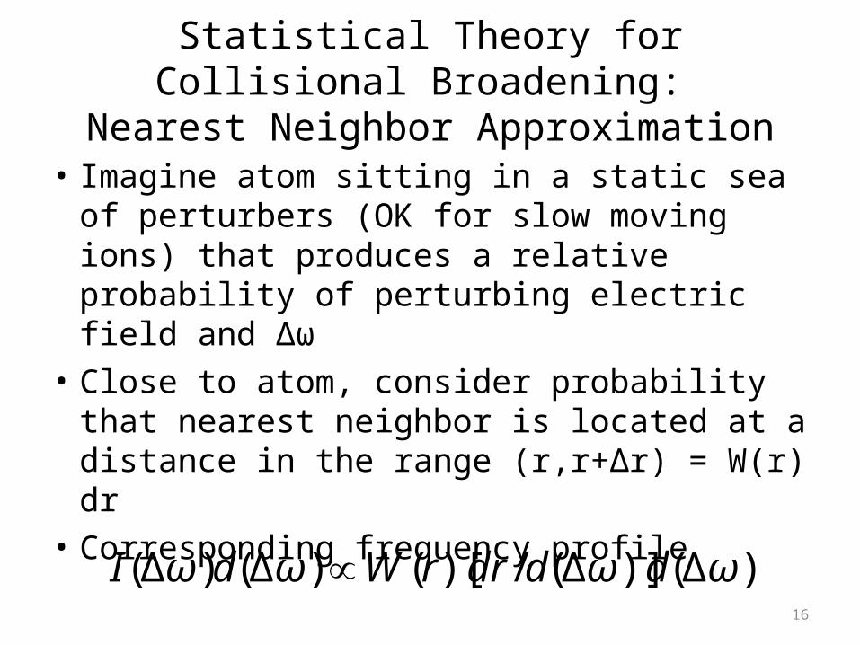
Statistical Theory for Collisional Broadening: Nearest Neighbor Approximation

• Imagine atom sitting in a static sea of perturbers (OK for slow moving ions) that produces a relative probability of perturbing electric field and Δω

• Close to atom, consider probability that nearest neighbor is located at a distance in the range (r,r+Δr) = W(r) dr

• Corresponding frequency profile

16

€

I(Δω)d(Δω) ∝W (r)[dr /d(Δω)]d(Δω)

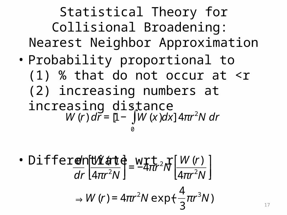
Statistical Theory for Collisional Broadening: Nearest Neighbor Approximation

• Probability proportional to (1) % that do not occur at <r (2) increasing numbers at increasing distance

• Differentiate wrt r

17

€

W (r) dr = [1 − W (x)dx0

r

∫ ] 4πr2N dr

€

d

dr

W (r)

4πr2N

⎡ ⎣ ⎢

⎤ ⎦ ⎥= −4πr2N

W (r)

4πr2N

⎡ ⎣ ⎢

⎤ ⎦ ⎥

⇒ W (r) = 4πr2N exp(−4

3πr3N)

Statistical Theory for Collisional Broadening: Nearest Neighbor Approximation

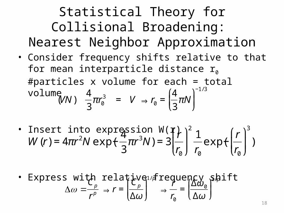
• Consider frequency shifts relative to that for mean interparticle distance r0 #particles x volume for each = total volume

• Insert into expression W(r)

• Express with relative frequency shift

18

€

(VN)4

3πr0

3 = V ⇒ r0 =4

3πN

⎛

⎝ ⎜

⎞

⎠ ⎟−1/ 3

€

W (r) = 4πr2N exp(−4

3πr3N) = 3

r

r0

⎛

⎝ ⎜

⎞

⎠ ⎟

21

r0exp(−

r

r0

⎛

⎝ ⎜

⎞

⎠ ⎟

3

)

€

Δω =Cp

r p ⇒ r =Cp

Δω

⎛

⎝ ⎜

⎞

⎠ ⎟

1/ p

⇒r

r0=

Δω0

Δω

⎛

⎝ ⎜

⎞

⎠ ⎟

1/ p

Statistical Theory for Collisional Broadening: Nearest Neighbor Approximation

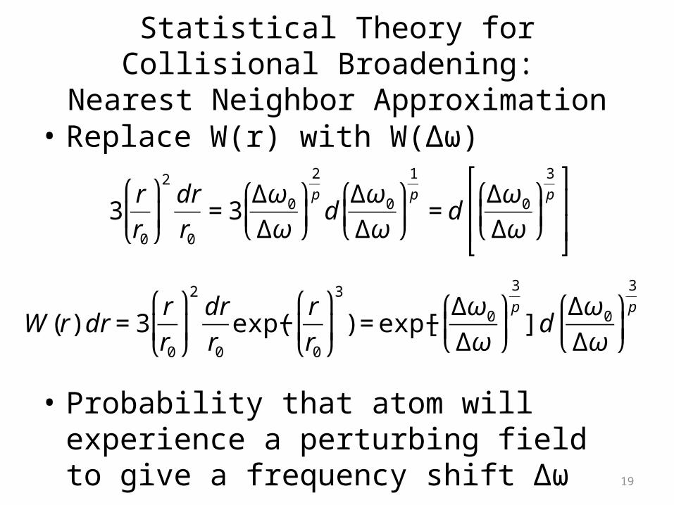
• Replace W(r) with W(Δω)

• Probability that atom will experience a perturbing field to give a frequency shift Δω

19

€

3r

r0

⎛

⎝ ⎜

⎞

⎠ ⎟

2dr

r0= 3

Δω0

Δω

⎛

⎝ ⎜

⎞

⎠ ⎟

2

pd

Δω0

Δω

⎛

⎝ ⎜

⎞

⎠ ⎟

1

p= d

Δω0

Δω

⎛

⎝ ⎜

⎞

⎠ ⎟

3

p ⎡

⎣

⎢ ⎢

⎤

⎦

⎥ ⎥

€

W (r) dr = 3r

r0

⎛

⎝ ⎜

⎞

⎠ ⎟

2dr

r0exp(−

r

r0

⎛

⎝ ⎜

⎞

⎠ ⎟

3

) = exp[−Δω0

Δω

⎛

⎝ ⎜

⎞

⎠ ⎟

3

p] d

Δω0

Δω

⎛

⎝ ⎜

⎞

⎠ ⎟

3

p

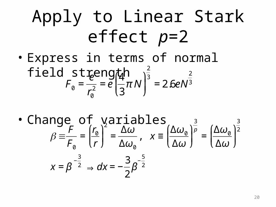
Apply to Linear Stark effect p=2

• Express in terms of normal field strength

• Change of variables

20

€

F0 =e

r02 = e

4

3π N

⎛

⎝ ⎜

⎞

⎠ ⎟

2

3= 2.6eN

2

3

€

β ≡F

F0

=r0r

⎛

⎝ ⎜

⎞

⎠ ⎟2

=Δω

Δω0

, x ≡Δω0

Δω

⎛

⎝ ⎜

⎞

⎠ ⎟

3

p=

Δω0

Δω

⎛

⎝ ⎜

⎞

⎠ ⎟

3

2

x = β−

3

2 ⇒ dx = −3

2β

−5

2

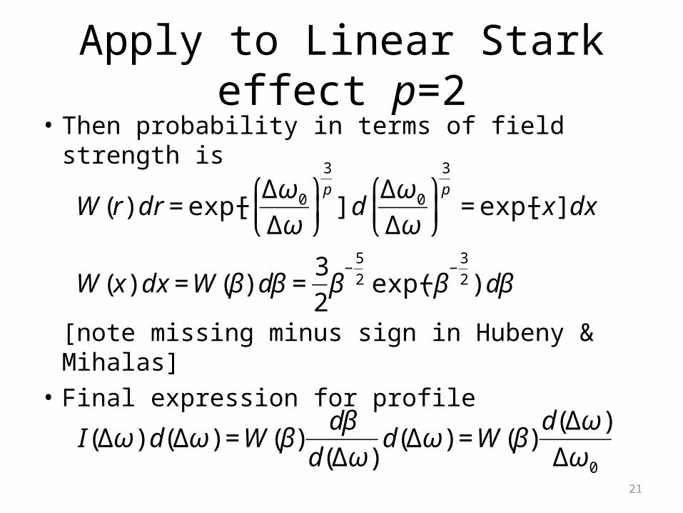
Apply to Linear Stark effect p=2• Then probability in terms of field strength is

[note missing minus sign in Hubeny & Mihalas]• Final expression for profile

21

€

W (r) dr = exp[−Δω0

Δω

⎛

⎝ ⎜

⎞

⎠ ⎟

3

p] d

Δω0

Δω

⎛

⎝ ⎜

⎞

⎠ ⎟

3

p= exp[−x] dx

W (x) dx =W (β) dβ =3

2β

−5

2 exp(−β−

3

2 ) dβ

€

I(Δω) d(Δω) =W (β)dβ

d(Δω)d(Δω) =W (β)

d(Δω)

Δω0

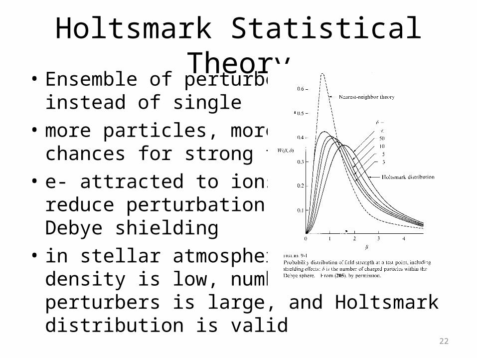
Holtsmark Statistical Theory• Ensemble of perturbers

instead of single• more particles, more

chances for strong field• e- attracted to ions,

reduce perturbation byDebye shielding

• in stellar atmospheres density is low, number of perturbers is large, and Holtsmark distribution is valid

22

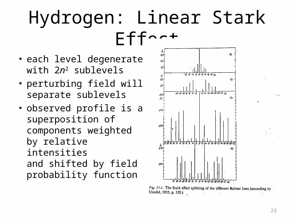
Hydrogen: Linear Stark Effect

• each level degeneratewith 2n2 sublevels

• perturbing field will separate sublevels

• observed profile is a superposition of components weighted by relative intensities and shifted by field probability function

23

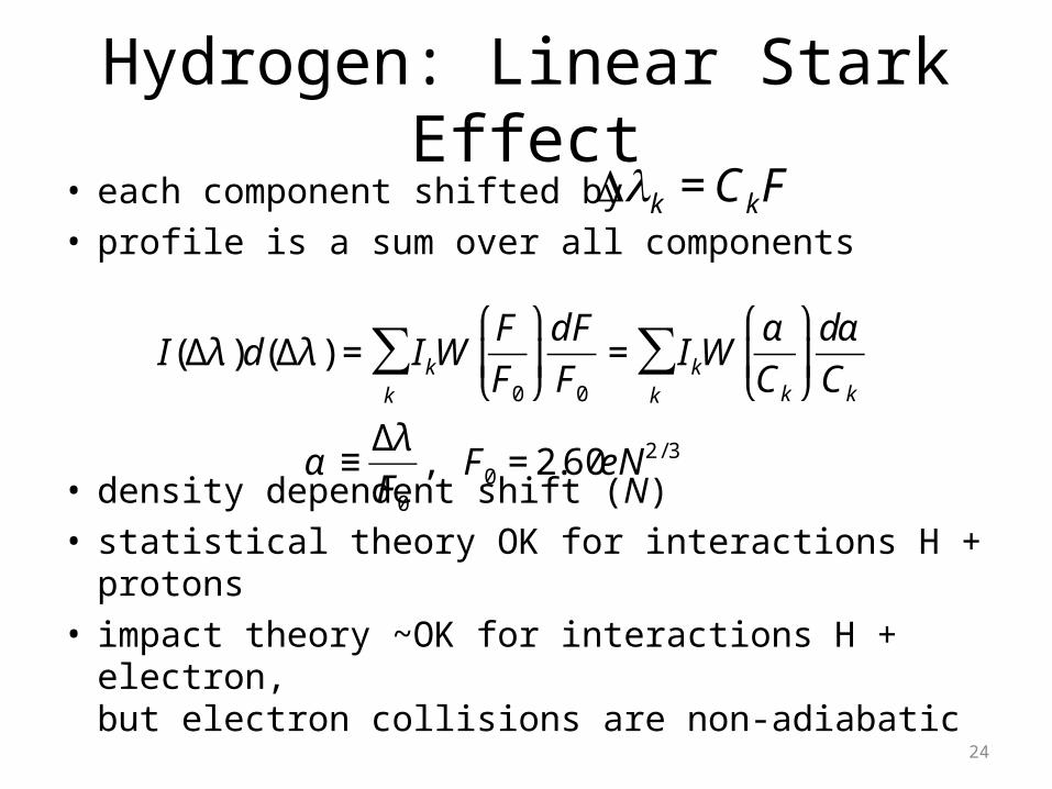
Hydrogen: Linear Stark Effect• each component shifted by • profile is a sum over all components

• density dependent shift (N)• statistical theory OK for interactions H + protons• impact theory ~OK for interactions H + electron,

but electron collisions are non-adiabatic24

€

I(Δλ )d(Δλ ) = IkWF

F0

⎛

⎝ ⎜

⎞

⎠ ⎟dF

F0k

∑ = IkWα

Ck

⎛

⎝ ⎜

⎞

⎠ ⎟dα

Ckk

∑

α ≡Δλ

F0

, F0 = 2.60eN 2 / 3

€

Δλk =CkF

Quantum Calculations for theLinear Stark effect of Hydrogen

• unified theory for electron and proton broadening for Lyman and Balmer series: Vidal, Cooper, & Smith 1973, ApJS, 25, 37

• IR seriesLemke 1997, A&AS, 122, 285

• Model Microfield Method (not static for ions)Stehle & Hutcheon 1999, A&AS, 140, 93

25

Summary

• final profile is a convolution of all the key broadening processes

• convolution of Lorentzian profiles: Γtotal=ΣΓi

• convolution of Lorentzian and Doppler broadening yields a Voigt profile

• convolution of Stark profile with Voigt (for H)• calculate as a function of depth in atmosphere

because broadening depends on T, N (Ne)

26