Spfirst l09 Ev

Copyright © Monash University 2009

Signal Processing

First

Lecture 9D‐to‐A Conversion

1


READING ASSIGNMENTS

• This Lecture:– Chapter 4: Sections 4‐4, 4‐5

• Other Reading:– Recitation: Section 4‐3 (Strobe Demo)– Next Lecture: Chapter 5 (beginning)

2


LECTURE OBJECTIVES

• DIGITAL‐to‐ANALOG CONVERSION is– Reconstruction from samples

• SAMPLING THEOREM applies

– Smooth Interpolation

• Mathematical Model of D‐to‐A– SUM of SHIFTED PULSES

• Linear Interpolation example

3


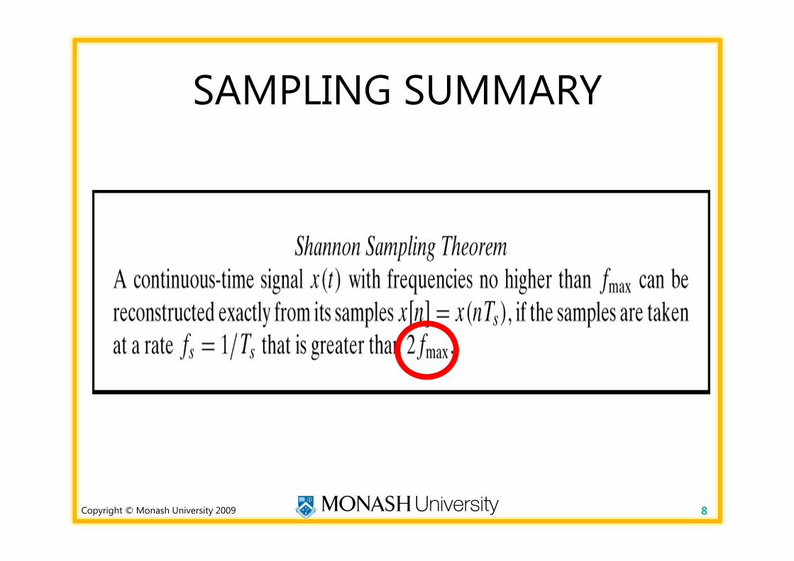
SAMPLING SUMMARY

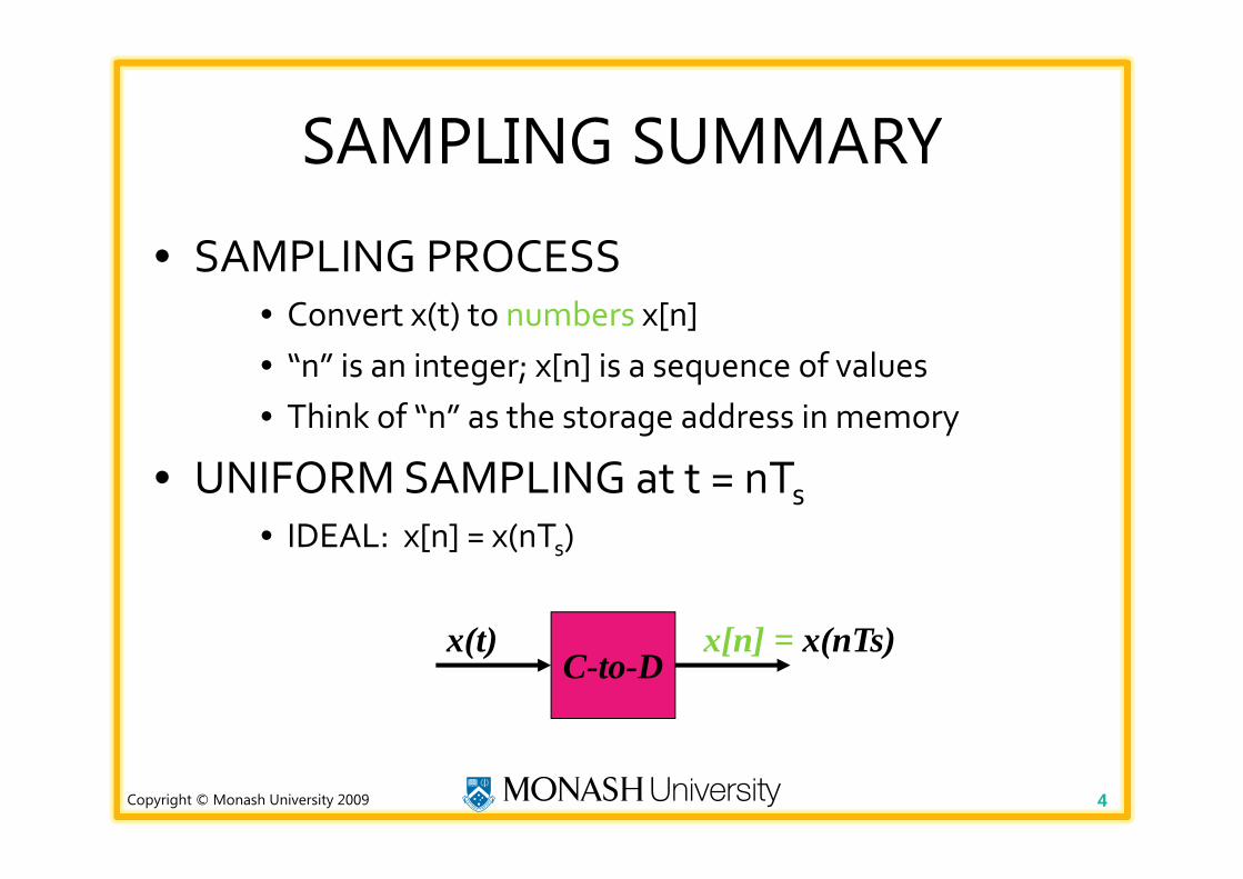
• SAMPLING PROCESS• Convert x(t) to numbers x[n]• “n” is an integer; x[n] is a sequence of values• Think of “n” as the storage address in memory

• UNIFORM SAMPLING at t = nTs• IDEAL: x[n] = x(nTs)

4

C-to-Dx(t) x[n] = x(nTs)


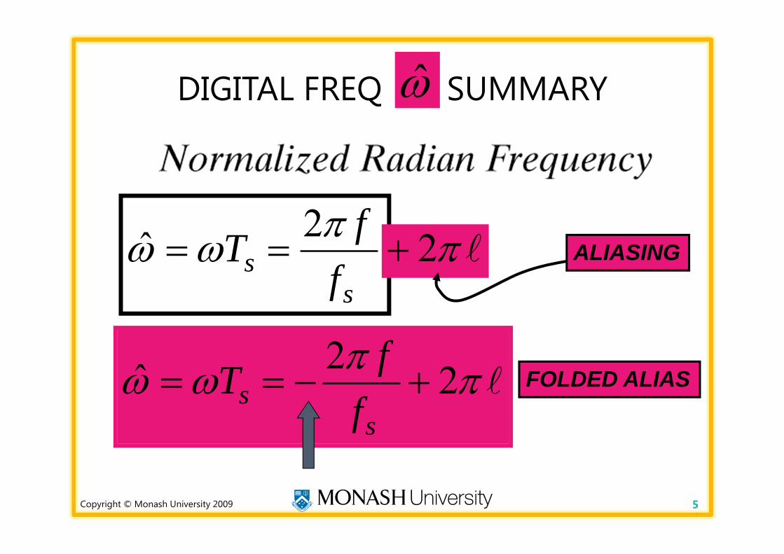
DIGITAL FREQ SUMMARY

5

ss f

fT 2ˆ 2

22ˆ s

s ffT FOLDED ALIAS

ALIASING


SPECTRUM (DIGITAL) SUMMARY

• Spectrum of x[n] has more than one line for each complex exponential– ALIASING, FOLDED ALIAS

• SPECTRUM is PERIODIC with period = 2

• PRINCIPAL (MINIMUM) ALIAS IN [‐– SAMPLING GUI (con2dis) demo

6


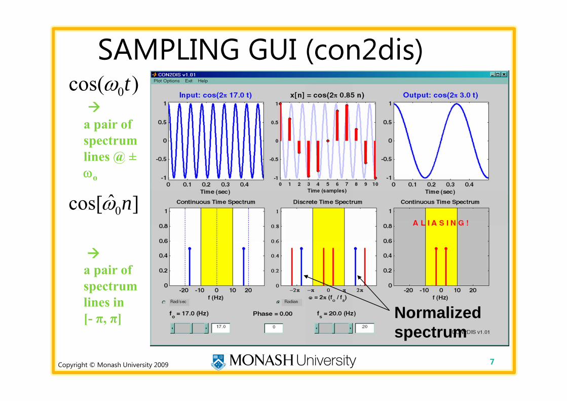
a pair of spectrum lines @ ±o

a pair of spectrum lines in[- π, π]

SAMPLING GUI (con2dis)

7

]ˆcos[ 0n

)cos( 0t

Normalizedspectrum


SAMPLING SUMMARY

8


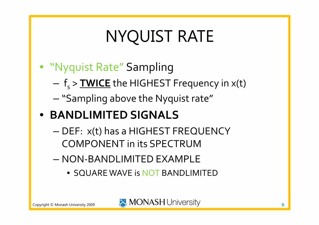
NYQUIST RATE

• “Nyquist Rate” Sampling– fs > TWICE the HIGHEST Frequency in x(t)– “Sampling above the Nyquist rate”

• BANDLIMITED SIGNALS– DEF: x(t) has a HIGHEST FREQUENCY COMPONENT in its SPECTRUM

– NON‐BANDLIMITED EXAMPLE• SQUARE WAVE is NOT BANDLIMITED

9


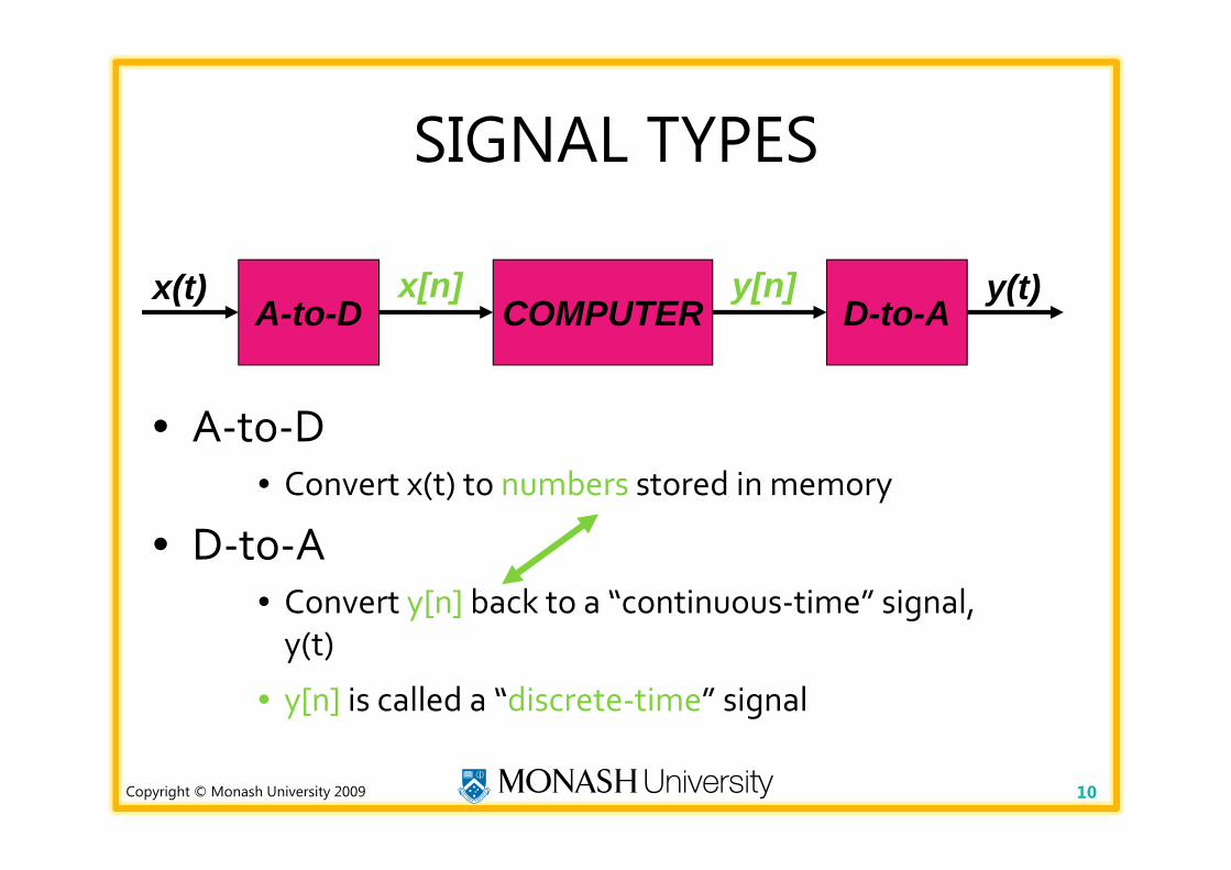
SIGNAL TYPES

• A‐to‐D• Convert x(t) to numbers stored in memory

• D‐to‐A• Convert y[n] back to a “continuous‐time” signal, y(t)

• y[n] is called a “discrete‐time” signal

10

COMPUTER D-to-AA-to-Dx(t) y(t)y[n]x[n]


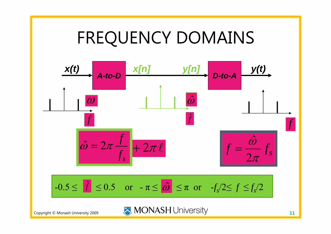
FREQUENCY DOMAINS

11

D-to-AA-to-Dx(t) y(t)x[n]

ff

f

y[n]

sff2ˆ

2sff 2ˆ

-0.5 ≤ ≤ 0.5 or - π ≤ ≤ π or -fs/2≤ f ≤ fs/2f


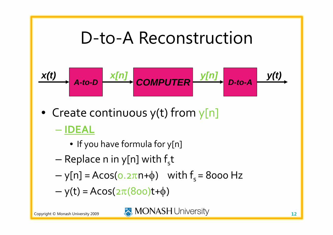
D-to-A Reconstruction

• Create continuous y(t) from y[n]– IDEAL

• If you have formula for y[n]

– Replace n in y[n] with fst– y[n] = Acos(0.2n+) with fs = 8000 Hz– y(t) = Acos(2(800)t+)

12

COMPUTER D-to-AA-to-Dx(t) y(t)y[n]x[n]


D-to-A is AMBIGUOUS !• ALIASING

– Given y[n], which y(t) do we pick ? ? ?– INFINITE NUMBER of y(t)

• PASSING THRU THE SAMPLES, y[n]

– D‐to‐A RECONSTRUCTION MUST CHOOSE ONE OUTPUT

• RECONSTRUCT – THE SMOOTHESTONE– THE LOWEST FREQ, if y[n] = sinusoid

13


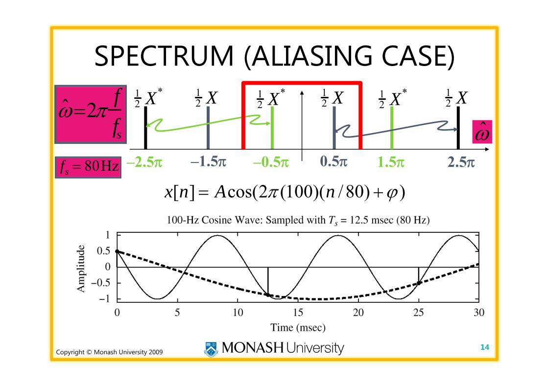
SPECTRUM (ALIASING CASE)

14

ˆ 2ffs

fs 80Hz

12 X*

–0.5

12 X

–1.5

12 X

0.5 2.5–2.5

ˆ

12 X1

2 X* 12 X*

1.5

))80/)(100(2cos(][ nAnx


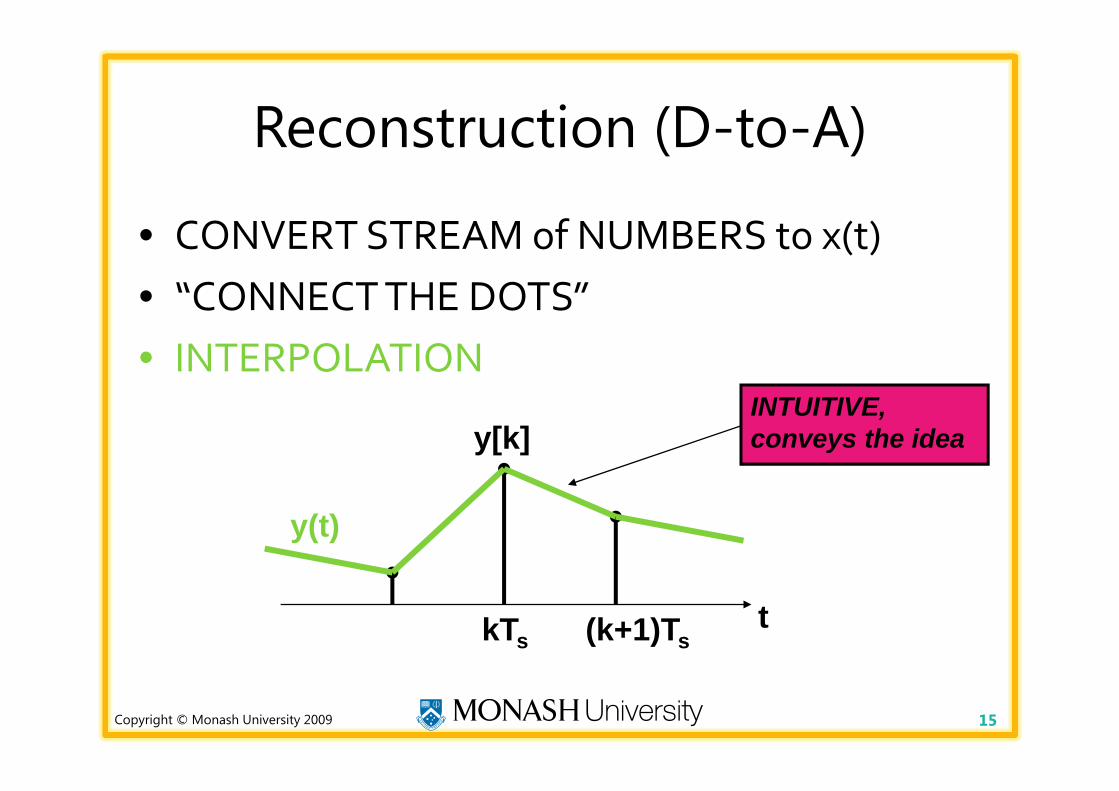
Reconstruction (D-to-A)

• CONVERT STREAM of NUMBERS to x(t)• “CONNECT THE DOTS”• INTERPOLATION

15

y(t)

y[k]

kTs (k+1)Tst

INTUITIVE,conveys the idea


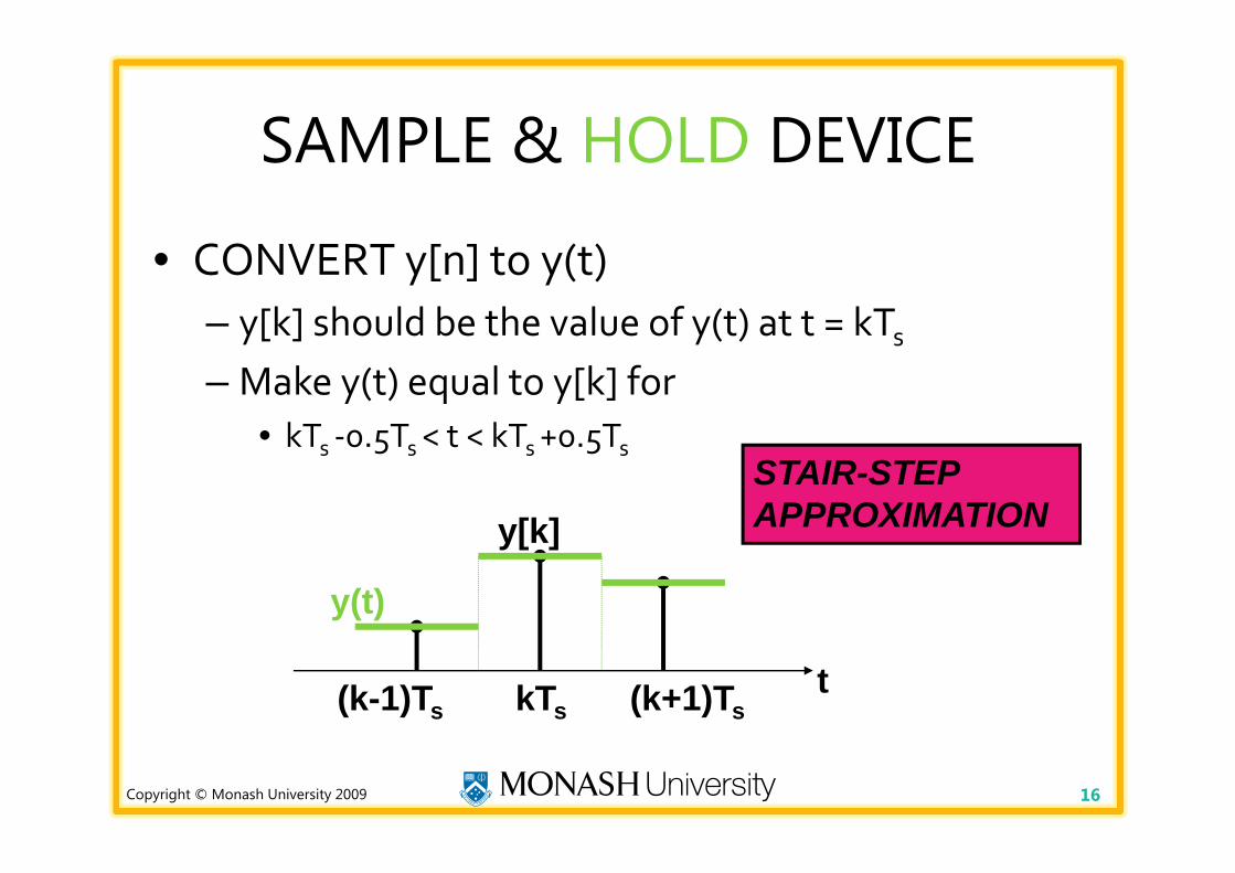
SAMPLE & HOLD DEVICE

• CONVERT y[n] to y(t)– y[k] should be the value of y(t) at t = kTs– Make y(t) equal to y[k] for

• kTs ‐0.5Ts < t < kTs+0.5Ts

16

y(t)

y[k]

kTs (k+1)Tst

STAIR-STEPAPPROXIMATION

(k-1)Ts


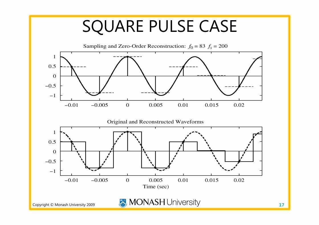
SQUARE PULSE CASE

17


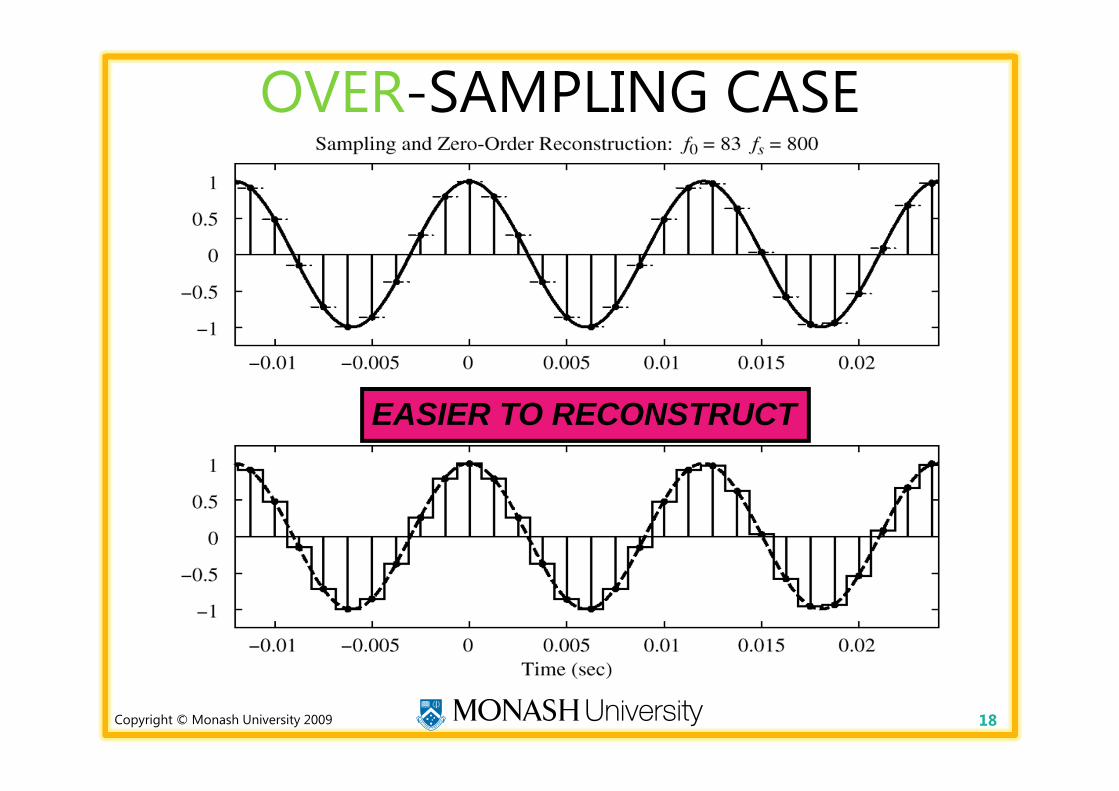
OVER-SAMPLING CASE

18

EASIER TO RECONSTRUCT


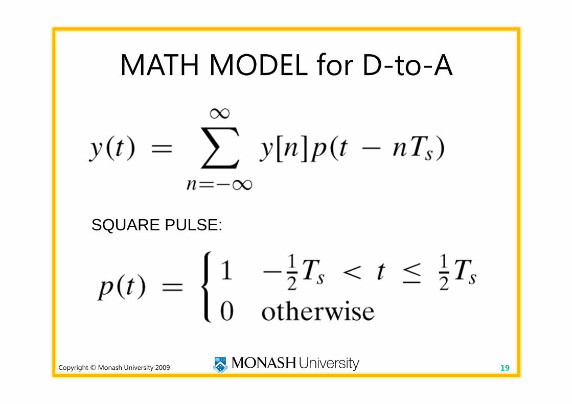
MATH MODEL for D-to-A

19

SQUARE PULSE:


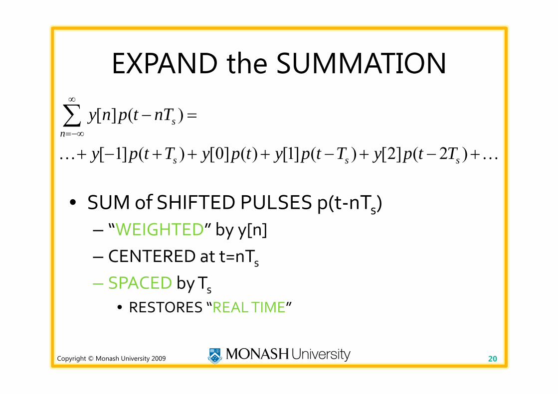
EXPAND the SUMMATION

• SUM of SHIFTED PULSES p(t‐nTs)– “WEIGHTED” by y[n]– CENTERED at t=nTs– SPACED by Ts

• RESTORES “REAL TIME”

20

[ ] ( )

[ 1] ( ) [0] ( ) [1] ( ) [2] ( 2 )

sn

s s s

y n p t nT

y p t T y p t y p t T y p t T

Copyright © Monash University 2009 21

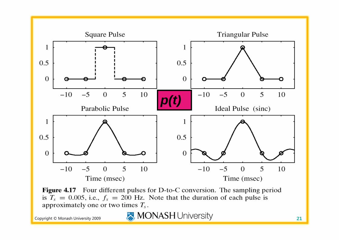
p(t)


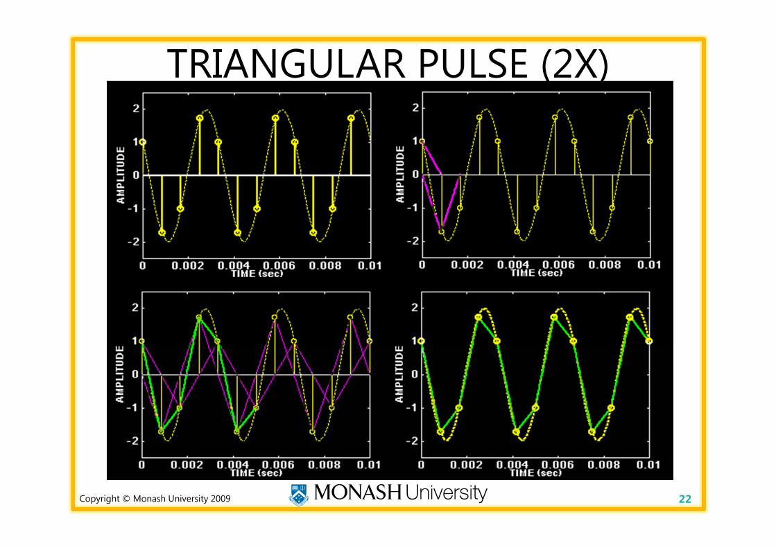
TRIANGULAR PULSE (2X)

22


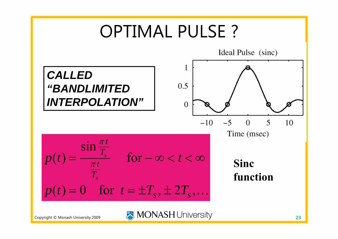
OPTIMAL PULSE ?

23

CALLED“BANDLIMITEDINTERPOLATION”

,2,for 0)(

for sin

)(

ss

TtT

t

TTttp

ttps

s

Sinc function


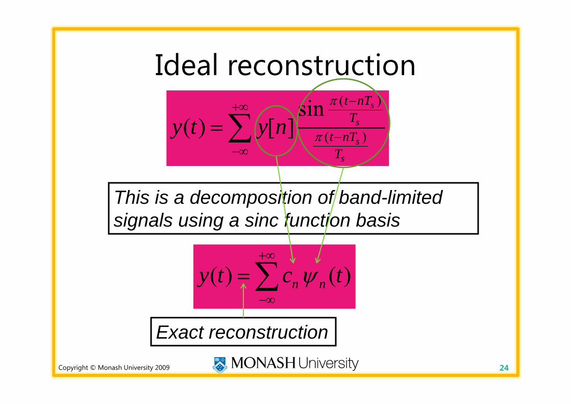
Ideal reconstruction

24

( )

( )

sin( ) [ ]

s

s

s

s

t nTT

t nTT

y t y n

( ) ( )n ny t c t

This is a decomposition of band-limited signals using a sinc function basis

Exact reconstruction

Documents

Spfirst l09 Ev