Embed Size (px)
Citation preview
Transportation Systems
Working Paper Series
Stated Preference Survey for New Smart
Transport Modes and Services:
Design, Pilot Study and New Revision
Paper# ITS-SCUSSE-09-02
March 2009
Lang Yang, Charisma F Choudhury & Moshe Ben-Akiva
Massachusetts Institute of Technology
João Abreu e Silva & Diana Carvalho
Instituto Superior Tecnico
March 2009 1
Stated Preference Survey for New Smart Transport Modes and Services: Design, Pilot Study and New Revision
MIT Portugal Program Transportation Systems Focus Area
Research Domain:
Intelligent Transportation Systems
Research Project: Smart Combination of Passenger Transport Modes and Services in Urban Areas for
Maximum System Sustainability and Efficiency (SCUSSE)
Paper#: ITS-SCUSSE-09-02
March 2009
Lang Yang ([email protected]), Charisma F Choudhury ([email protected]), Moshe Ben-Akiva ([email protected])
Intelligent Transportation Systems Lab
Department of Civil and Environmental Engineering Massachusetts Institute of Technology
João Abreu e Silva ([email protected]), Diana Carvalho ([email protected])
Instituto Superior Tecnico Universidade Tecnica de Lisbon, Protugal
This publication was made possible by the generous support of the Government of Portugal through the Portuguese Foundation for International Cooperation in Science, Technology and Higher Education and was undertaken in the MIT-Portugal Program.
March 2009 2
Contents
1 Introduction...............................................................................................................3
2 Preparatory Phase and Pilot Study .............................................................................6
2.1 Development of the SP Survey ...........................................................................6
2.1.1 Focus Group Discussion ..............................................................................6
2.1.2 Framing the Questions of the SP Survey ......................................................7
2.1.3 Experimental Design and Test.................................................................... 12
2.2 Data.................................................................................................................. 12
2.2.1 General Findings........................................................................................ 13
2.2.2 Respondent Characteristics ........................................................................ 14
2.2.3 RP Mode Choice Data................................................................................ 15
2.2.4 SP Mode Choice Data ................................................................................ 17
2.2.5 Departure Time Choice Data...................................................................... 18
2.3 Model Estimation ............................................................................................. 19
2.3.1 Mode Choice Model .................................................................................. 20
2.3.2 Departure Time Choice Model ................................................................... 27
2.4 Attitudes to Car and Public Transportation........................................................ 30
2.5 Information Services......................................................................................... 35
3 Revised Stated Preference Survey............................................................................ 36
3.1 Main Adjustments from Pilot Study.................................................................. 36
3.2 Updated SP Scenarios with Multidimensional Choice....................................... 36
3.3 Updates in the Experimental Design ................................................................. 41
4 Future Plans and Challenges.................................................................................... 43
References .................................................................................................................... 45
Appendix A................................................................................................................... 47
March 2009 3
1 Introduction
New Smart Transport Modes and Services The objective of SCUSSE (Smart Combination of Passenger Transport Modes and Services in Urban Areas for Maximum System Sustainability and Efficiency) is to conceive, organize and simulate the implementation of new smart transport modes and services to optimize integration with lifestyles and to improve the sustainability and efficiency for urban transport systems, including the institutional design required for and/or enabled by the deployment of innovative services. The existing modes of day-to-day travel in Lisbon primarily include car (as a driver, normal passenger or car-pool user), bus and heavy modes like subway, train and ferry. Some of the journeys are made by a combination of these modes as well (e.g. bus and heavy mode, car and heavy mode) etc. SCUSSE investigates different aspects of improving the existing modes as well as introduction of new smart transport modes in order to improve the efficiency of urban transport systems. The new transport modes investigated in this study include the following: ! One-way car rental This service provides access to light electric vehicles available at nearby parking lots throughout the city placed in closely spaced intervals. Travelers can simply walk to a nearest lot, swipe a card to pick up a vehicle, drive it to the lot nearest to your destination, and drop it off there. The insurance, service, repair, fuel and parking costs are included in the rental price and service package. Parking spots are also guaranteed for the service users at the destinations. This mode is more convenient and less expensive compared to a typical rental car. Service users need to keep some money (or provide credit card number) as a caution. ! Shared taxi This service provides a taxi service with call-centre dispatch access. Upon boarding, a passenger is asked whether he/she is willing to share the taxi with other passengers who have similar routes. If he/she agrees, other passengers will board the taxi until the vehicle capacity is reached. The fare will be determined based on the most convenient distance (on a solo trip) and the time penalty endured for the sake of the other passengers. This mode is less expensive compared to a typical taxi service. ! Express minibus This service provides a minibus service with fixed routes, few stops near the origin and the destination (2 or 3 at most), and a significant stretch in between. The minibus has a regular and pre-programmed schedule. This transport mode mainly focuses on frequent commuters that live and work close to rather convenient places, who can share a collective pick-up location and destination. There may be a few places available for occasional riders as well. The minibus service is only available during peak periods 8:00 to 10:30 in the morning and 16:30 to 20:00 in the afternoon. ! Park and ride with child drop-off
March 2009 4
This service provides access to park and ride facilities with reserved parking spaces, where commuters can leave their car and board a subway/train/ferry. In addition, there is panoply of other services such as children drop-off (where children less than 10 years old can be dropped off to be picked up by professional tutors). The tutors will be reliable persons chosen collectively (either school teachers or professional people) and will take care of the children before taking them to their school in school buses. There will be a monthly charge associated with the service. New traffic management methods include the following:
! Congestion pricing policies that apply charges based on departure time ! Adjustment of parking pricing and enforcement. ! New information services, including Internet or cell phone based traffic
information, and GPS navigation systems that can be used to predicate travel time and reduce the time variability.
Motivation of Stated Preference Survey Stated Preference (SP) surveys, also called self-stated preferences for market products or services, have been widely applied in the areas of marketing and travel demand modeling, separately or jointly with Revealed Preference (RP) surveys with observed choices of product purchase or service use. It is an efficient method to analyze consumers’ evaluation of multi-attributed products and services, especially when there are hypothetical choice alternatives and new attributes. In the case of Lisbon, Portugal, there are no Revealed Preference (RP) data for the proposed innovative transport modes and information services, and there are no existing congestion pricing strategies in urban areas. Therefore, a Stated Preference (SP) survey must be well designed and implemented for our objectives, such as
! To evaluate acceptability of innovative modes and services ! To quantify sensitivity to level of service by varying values of access time,
waiting time, travel time, cost etc. ! To measure willingness-to-pay ! To investigate effects of attitudes and perceptions.
Challenges and Complexity There are current transport modes, innovative transport modes, and also new combinations of existing and innovative. The result is a large choice set for a particular origin-destination. The ten most probable choice sets are as follows
1:
! Driving alone in a private car ! Carpool ! Bus ! Heavy mode ! Bus and heavy mode
1 The less probable combinations are excluded for simplicity
March 2009 5
! One-way car rental ! Shared taxi ! Express minibus ! Park & ride (with or without child drop-off), and ! One-way car rental with heavy mode.
There are numerous attributes that need to be considered for these alternatives. Furthermore, new smart services introduced in Lisbon include congestion pricing, adjustment of parking pricing and enforcement, and information services such as Internet, cell phone and GPS navigation systems. They will affect the accuracy of travel time predication and people’s time-of-day preference. The SP survey should include corresponding attributes and alternatives to capture such effects. In addition, these alternatives are not uniform in format (e.g. waiting time is applicable to public transport modes only, parking is associated with car only etc.). Therefore, the organization and presentation of these alternatives and attributes is a challenge for the Stated Preference (SP) survey. An additional challenge was to accommodate the availability of modes (not all modes are available for all origin destination pairs) and the base value of attributes for a certain mode (which are context dependent). Also, the success of the survey depended on how realistically the survey can be presented so that potential biases in the data are minimized. The process of developing the SP survey is summarized in seven steps:
1. Defining important attributes 2. Designing the questionnaire of SP survey 3. Experimental design 4. Testing with synthetic data 5. Pilot study and analysis 6. Revising SP survey 7. Implementation of Internet survey and supplemental presential survey
Structure of This Paper The remainder of this paper is organized as follows. Section 2 describes the preparatory and testing phase of the main survey: this includes summary of the focus group study and its findings, detailing the experimental design method, developing the Pilot version of the Stated Preference survey and testing it using a small number of respondents. Findings of simple discrete choice models estimated with Pilot data are also presented in this context. Section 3 discusses the revised version of the SP survey and associated design modifications. Section 4 talks about future plans and modeling challenges.
March 2009 6
2 Preparatory Phase and Pilot Study
The SP survey included ten alternatives, five of which are new smart alternatives or combination of exiting and smart alternatives. Each of the alternatives involves numerous attributes and a focus group study was conducted first to identify the more preferred attributes. The findings of this focus group study were the basis of designing the preliminary or Pilot version of the survey, which was tested with 150 respondents. This section presents summary of the focus group study and its findings, the framework of the survey and the selected experimental design method and statistical analysis of the Pilot data followed by findings of simple discrete choice models estimated with this data.
2.1 Development of the SP Survey
2.1.1 Focus Group Discussion
A focus group discussion was conducted March 2008 in Lisbon, Portugal. The objectives were to find aspects of public transport, car, the new alternative modes and services that could act as attraction or repulsion factors, to identify important attributes characterizing the new services that may be used in the SP survey, and to identify potential attitudinal aspects that could be included in the SP survey. The main findings of the focus group discussion are as follows (see Viegas et al, 2008 for a more in-depth description of this focus group results). Carpool - not culturally adapted to the Portuguese
! Advantages: low costs and environmentally friendly ! Disadvantages: loss of independence and the possibility of conflicts
Shared Taxis - good receptivity ! Advantages: low price, environmentally friendly, good option when public
transport was not frequent ! Disadvantages: long travel time, lack of reliability and security
Minibus - good receptivity ! Advantages: comfort ! Disadvantages: less flexibility and high costs
Park & Ride with child drop-off - skepticism ! Advantages: connected with park and ride, good option for people who did not
mind leaving their children with others ! Disadvantages: lack of security for children, lack of confidence in tutors and
drivers Congestion charge - mixed feelings
! In principle people agreed with this measure ! Approval depended on how to use the collected money and the necessity to
provide some kind of support to the ones that have an absolute need to use their cars
Information systems
March 2009 7
! Reliability and precision was an important issue ! Information should provide data for inter-modal options
When choosing among transport modes and services, we found the important attributes for the local residents were travel time, time variability, travel cost, frequency, the reliability of tutors for park & ride with child drop-off, etc. There also existed some attitudinal factors possibly to affect people’ preference, such as comfort, privacy, flexibility, convenience, environmental friendly, and security.
2.1.2 Framing the Questions of the SP Survey
The large questionnaire of SP survey was divided into five parts: (1) Socio-economic information and current travel behavior/ RP data, (2) SP choice scenarios, including scenarios 1 and 2 only with travel mode choice, and scenario 3 with travel mode choice as well as departure time choice when the trip is flexible, (3) Information services, (4) Diagnostic questions, (5) Attitudes and perceptions.
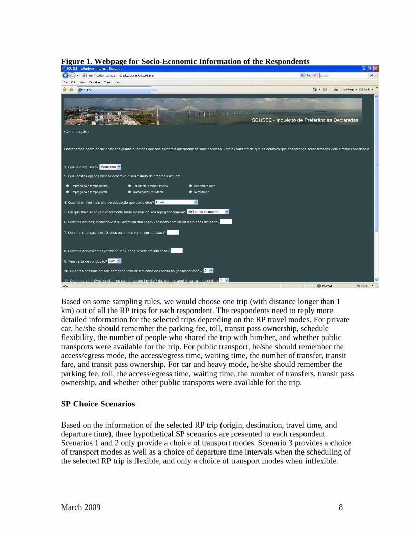
Current Travel Behavior The first step is to collect the socio-economic information of the respondents, such as individual characteristics (age, gender, occupation, education, and driver license), household composition (children, teenagers and adults), income levels, residential location, car ownership, parking availability and conditions, and transit pass ownership. The respondents are then asked to recall all the trips that they have made during yesterday or the last weekday, and provide origins, destinations, start time, end time, transport modes, distance and purposes for all these trips (Revealed Preference data). Figure 1 presents a sample webpage of the questions regarding the respondents’ socio-economic information (in Portuguese).
March 2009 8
Figure 1. Webpage for Socio-Economic Information of the Respondents
Based on some sampling rules, we would choose one trip (with distance longer than 1 km) out of all the RP trips for each respondent. The respondents need to reply more detailed information for the selected trips depending on the RP travel modes. For private car, he/she should remember the parking fee, toll, transit pass ownership, schedule flexibility, the number of people who shared the trip with him/her, and whether public transports were available for the trip. For public transport, he/she should remember the access/egress mode, the access/egress time, waiting time, the number of transfer, transit fare, and transit pass ownership. For car and heavy mode, he/she should remember the parking fee, toll, the access/egress time, waiting time, the number of transfers, transit pass ownership, and whether other public transports were available for the trip.
SP Choice Scenarios
Based on the information of the selected RP trip (origin, destination, travel time, and departure time), three hypothetical SP scenarios are presented to each respondent. Scenarios 1 and 2 only provide a choice of transport modes. Scenario 3 provides a choice of transport modes as well as a choice of departure time intervals when the scheduling of the selected RP trip is flexible, and only a choice of transport modes when inflexible.
March 2009 9
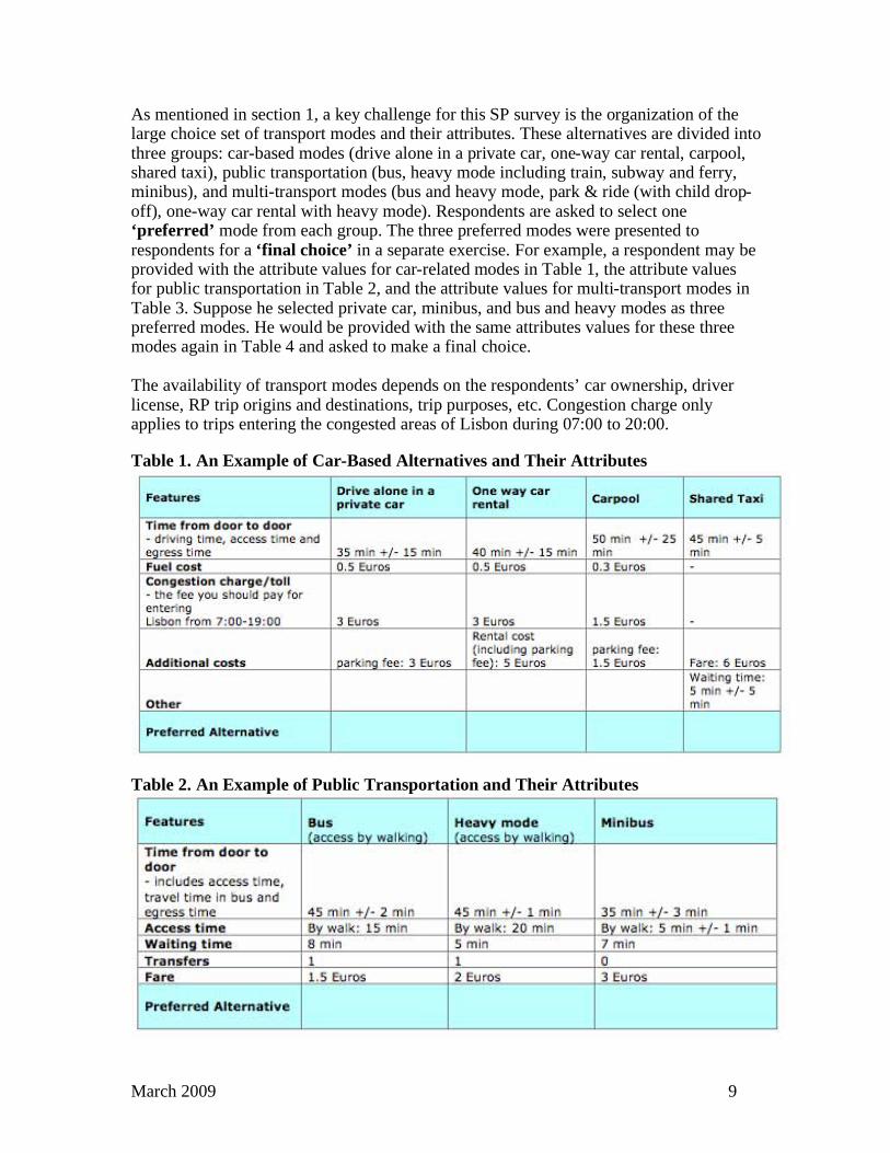
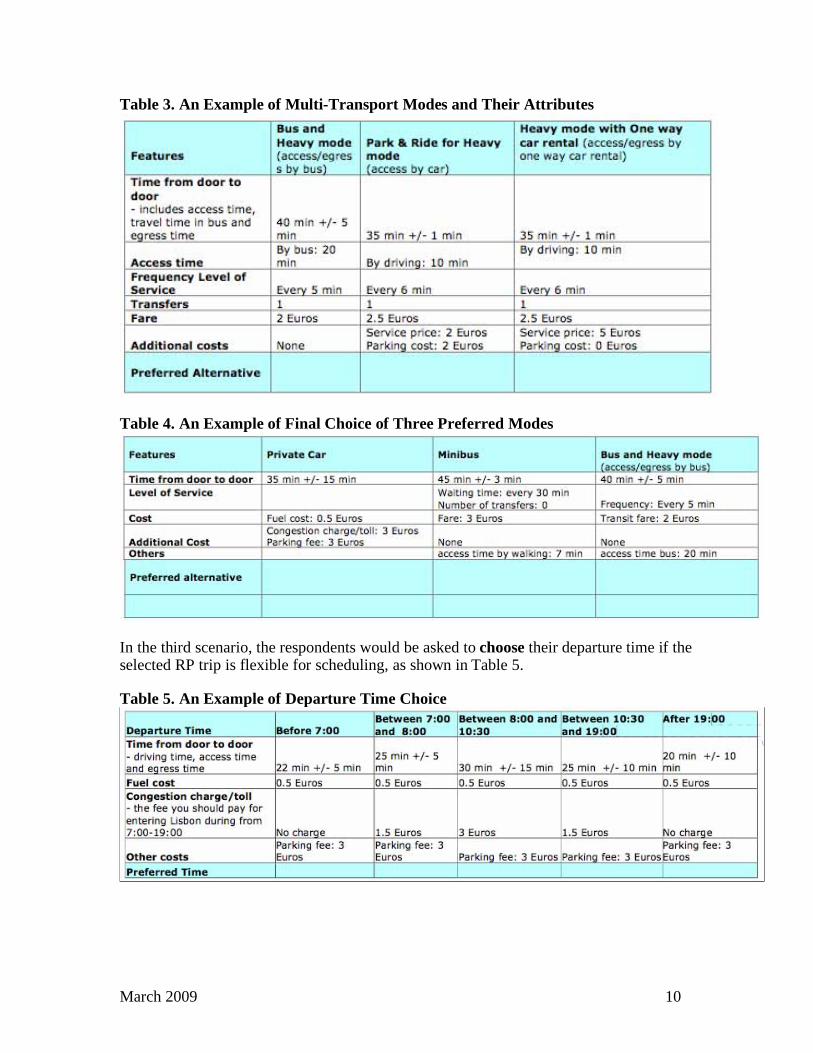
As mentioned in section 1, a key challenge for this SP survey is the organization of the large choice set of transport modes and their attributes. These alternatives are divided into three groups: car-based modes (drive alone in a private car, one-way car rental, carpool, shared taxi), public transportation (bus, heavy mode including train, subway and ferry, minibus), and multi-transport modes (bus and heavy mode, park & ride (with child drop-off), one-way car rental with heavy mode). Respondents are asked to select one ‘preferred’ mode from each group. The three preferred modes were presented to respondents for a ‘final choice’ in a separate exercise. For example, a respondent may be provided with the attribute values for car-related modes in Table 1, the attribute values for public transportation in Table 2, and the attribute values for multi-transport modes in Table 3. Suppose he selected private car, minibus, and bus and heavy modes as three preferred modes. He would be provided with the same attributes values for these three modes again in Table 4 and asked to make a final choice. The availability of transport modes depends on the respondents’ car ownership, driver license, RP trip origins and destinations, trip purposes, etc. Congestion charge only applies to trips entering the congested areas of Lisbon during 07:00 to 20:00.
Table 1. An Example of Car-Based Alternatives and Their Attributes
Table 2. An Example of Public Transportation and Their Attributes
March 2009 10
Table 3. An Example of Multi-Transport Modes and Their Attributes
Table 4. An Example of Final Choice of Three Preferred Modes
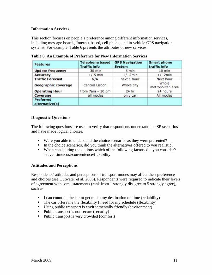
In the third scenario, the respondents would be asked to choose their departure time if the selected RP trip is flexible for scheduling, as shown in Table 5.
Table 5. An Example of Departure Time Choice
March 2009 11
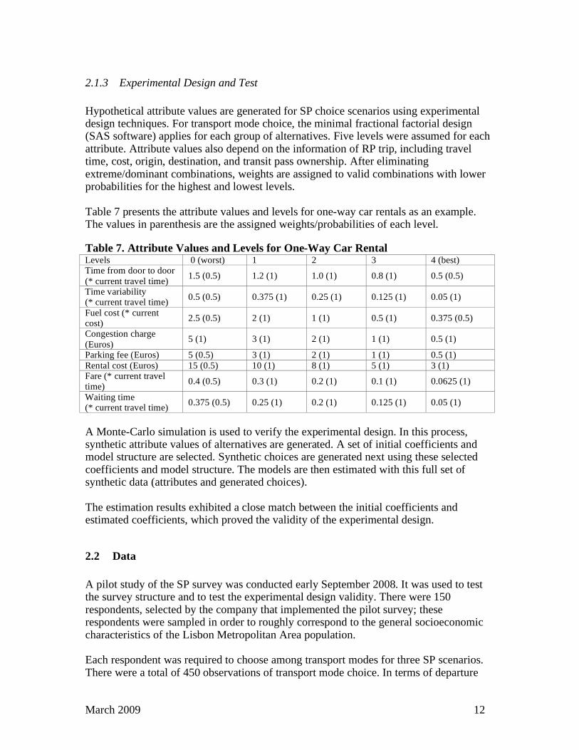
Information Services This section focuses on people’s preference among different information services, including message boards, Internet-based, cell phone, and in-vehicle GPS navigation systems. For example, Table 6 presents the attributes of new services.
Table 6. An Example of Preference for New Information Services
Diagnostic Questions The following questions are used to verify that respondents understand the SP scenarios and have made logical choices.
! Were you able to understand the choice scenarios as they were presented? ! In the choice scenarios, did you think the alternatives offered to you realistic? ! When considering the options which of the following factors did you consider?
Travel time/cost/convenience/flexibility
Attitudes and Perceptions Respondents’ attitudes and perceptions of transport modes may affect their preference and choices (see Outwater et al. 2003). Respondents were required to indicate their levels of agreement with some statements (rank from 1 strongly disagree to 5 strongly agree), such as
! I can count on the car to get me to my destination on time (reliability) ! The car offers me the flexibility I need for my schedule (flexibility) ! Using public transport is environmentally friendly (environment) ! Public transport is not secure (security) ! Public transport is very crowded (comfort)
March 2009 12
2.1.3 Experimental Design and Test
Hypothetical attribute values are generated for SP choice scenarios using experimental design techniques. For transport mode choice, the minimal fractional factorial design (SAS software) applies for each group of alternatives. Five levels were assumed for each attribute. Attribute values also depend on the information of RP trip, including travel time, cost, origin, destination, and transit pass ownership. After eliminating extreme/dominant combinations, weights are assigned to valid combinations with lower probabilities for the highest and lowest levels. Table 7 presents the attribute values and levels for one-way car rentals as an example. The values in parenthesis are the assigned weights/probabilities of each level.
Table 7. Attribute Values and Levels for One-Way Car Rental Levels 0 (worst) 1 2 3 4 (best) Time from door to door
(* current travel time) 1.5 (0.5) 1.2 (1) 1.0 (1) 0.8 (1) 0.5 (0.5)
Time variability (* current travel time)
0.5 (0.5) 0.375 (1) 0.25 (1) 0.125 (1) 0.05 (1)
Fuel cost (* current cost)
2.5 (0.5) 2 (1) 1 (1) 0.5 (1) 0.375 (0.5)
Congestion charge
(Euros) 5 (1) 3 (1) 2 (1) 1 (1) 0.5 (1)
Parking fee (Euros) 5 (0.5) 3 (1) 2 (1) 1 (1) 0.5 (1)
Rental cost (Euros) 15 (0.5) 10 (1) 8 (1) 5 (1) 3 (1) Fare (* current travel time)
0.4 (0.5) 0.3 (1) 0.2 (1) 0.1 (1) 0.0625 (1)
Waiting time (* current travel time)
0.375 (0.5) 0.25 (1) 0.2 (1) 0.125 (1) 0.05 (1)
A Monte-Carlo simulation is used to verify the experimental design. In this process, synthetic attribute values of alternatives are generated. A set of initial coefficients and model structure are selected. Synthetic choices are generated next using these selected coefficients and model structure. The models are then estimated with this full set of synthetic data (attributes and generated choices). The estimation results exhibited a close match between the initial coefficients and estimated coefficients, which proved the validity of the experimental design.
2.2 Data
A pilot study of the SP survey was conducted early September 2008. It was used to test the survey structure and to test the experimental design validity. There were 150 respondents, selected by the company that implemented the pilot survey; these respondents were sampled in order to roughly correspond to the general socioeconomic characteristics of the Lisbon Metropolitan Area population. Each respondent was required to choose among transport modes for three SP scenarios. There were a total of 450 observations of transport mode choice. In terms of departure
March 2009 13
time choice, there were a total of 71 observations for respondents who had flexibility in trip scheduling.
2.2.1 General Findings
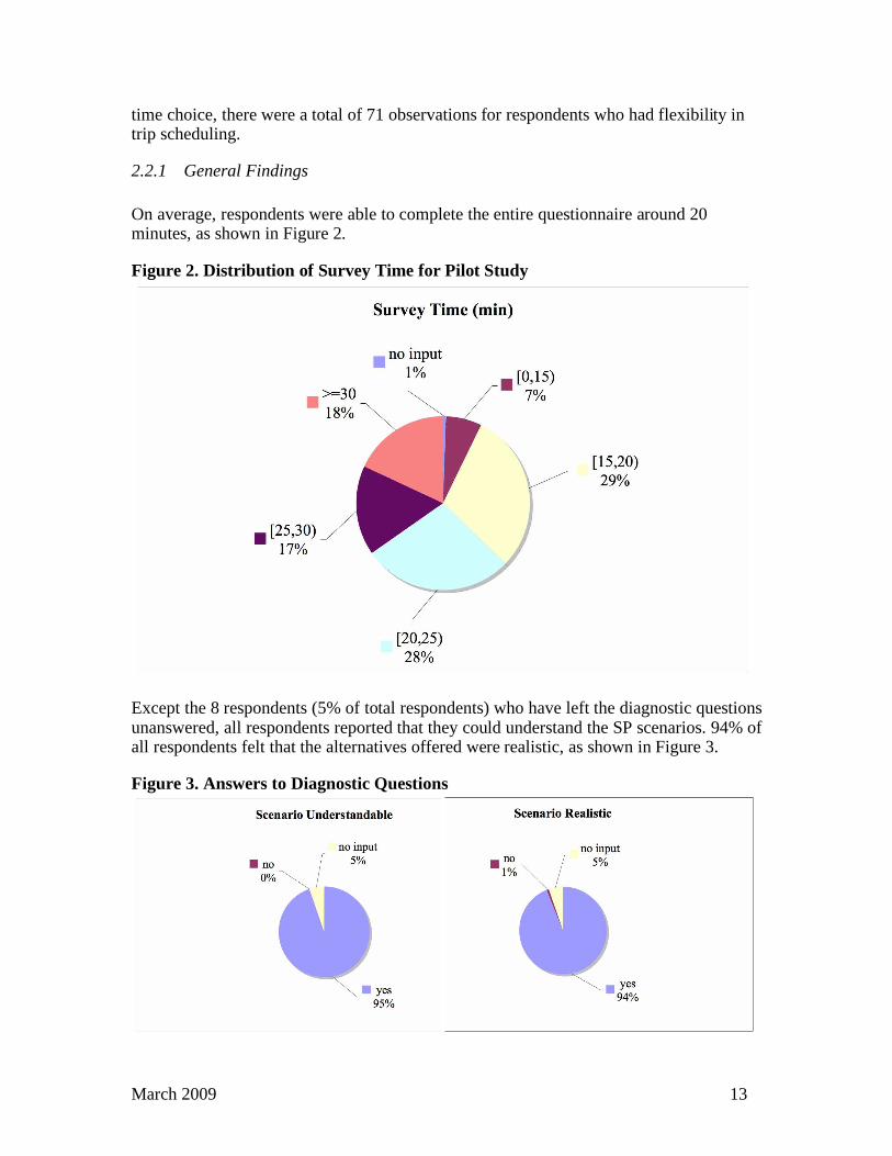
On average, respondents were able to complete the entire questionnaire around 20 minutes, as shown in Figure 2.
Figure 2. Distribution of Survey Time for Pilot Study
Except the 8 respondents (5% of total respondents) who have left the diagnostic questions unanswered, all respondents reported that they could understand the SP scenarios. 94% of all respondents felt that the alternatives offered were realistic, as shown in Figure 3.
Figure 3. Answers to Diagnostic Questions
March 2009 14
2.2.2 Respondent Characteristics
Here are some basic statistics about these respondents at the time of the survey,
! Most respondents were between the ages of 18 to 45 ! 50% of the respondents were female ! 141 respondents were employed full-time, 7 were employed part-time, and 2 were
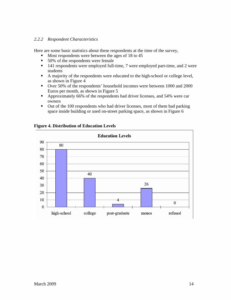
students ! A majority of the respondents were educated to the high-school or college level,
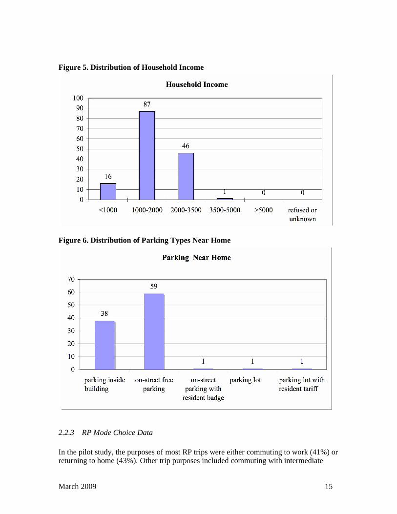
as shown in Figure 4 ! Over 50% of the respondents’ household incomes were between 1000 and 2000
Euros per month, as shown in Figure 5 ! Approximately 66% of the respondents had driver licenses, and 54% were car
owners ! Out of the 100 respondents who had driver licenses, most of them had parking
space inside building or used on-street parking space, as shown in Figure 6
Figure 4. Distribution of Education Levels
March 2009 15
Figure 5. Distribution of Household Income
Figure 6. Distribution of Parking Types Near Home
2.2.3 RP Mode Choice Data
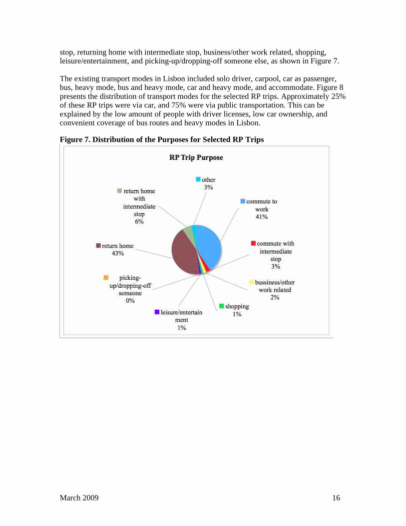
In the pilot study, the purposes of most RP trips were either commuting to work (41%) or returning to home (43%). Other trip purposes included commuting with intermediate
March 2009 16
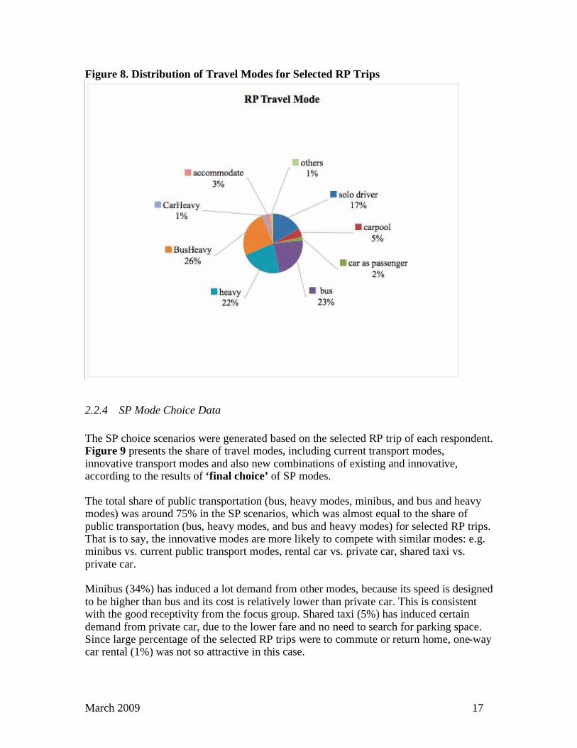
stop, returning home with intermediate stop, business/other work related, shopping, leisure/entertainment, and picking-up/dropping-off someone else, as shown in Figure 7. The existing transport modes in Lisbon included solo driver, carpool, car as passenger, bus, heavy mode, bus and heavy mode, car and heavy mode, and accommodate. Figure 8 presents the distribution of transport modes for the selected RP trips. Approximately 25% of these RP trips were via car, and 75% were via public transportation. This can be explained by the low amount of people with driver licenses, low car ownership, and convenient coverage of bus routes and heavy modes in Lisbon.
Figure 7. Distribution of the Purposes for Selected RP Trips
March 2009 17
Figure 8. Distribution of Travel Modes for Selected RP Trips
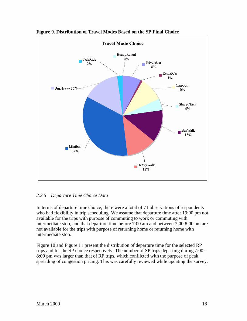
2.2.4 SP Mode Choice Data
The SP choice scenarios were generated based on the selected RP trip of each respondent. Figure 9 presents the share of travel modes, including current transport modes, innovative transport modes and also new combinations of existing and innovative, according to the results of ‘final choice’ of SP modes. The total share of public transportation (bus, heavy modes, minibus, and bus and heavy modes) was around 75% in the SP scenarios, which was almost equal to the share of public transportation (bus, heavy modes, and bus and heavy modes) for selected RP trips. That is to say, the innovative modes are more likely to compete with similar modes: e.g. minibus vs. current public transport modes, rental car vs. private car, shared taxi vs. private car. Minibus (34%) has induced a lot demand from other modes, because its speed is designed to be higher than bus and its cost is relatively lower than private car. This is consistent with the good receptivity from the focus group. Shared taxi (5%) has induced certain demand from private car, due to the lower fare and no need to search for parking space. Since large percentage of the selected RP trips were to commute or return home, one-way car rental (1%) was not so attractive in this case.
March 2009 18
Figure 9. Distribution of Travel Modes Based on the SP Final Choice
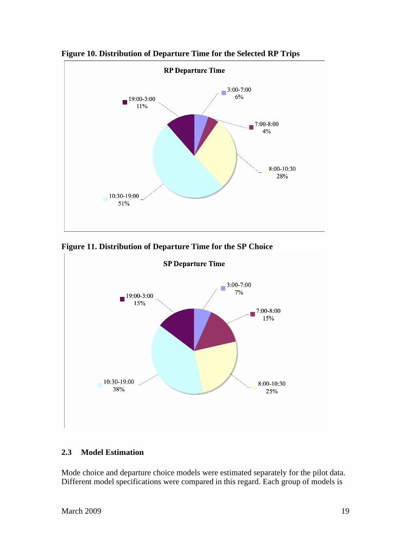
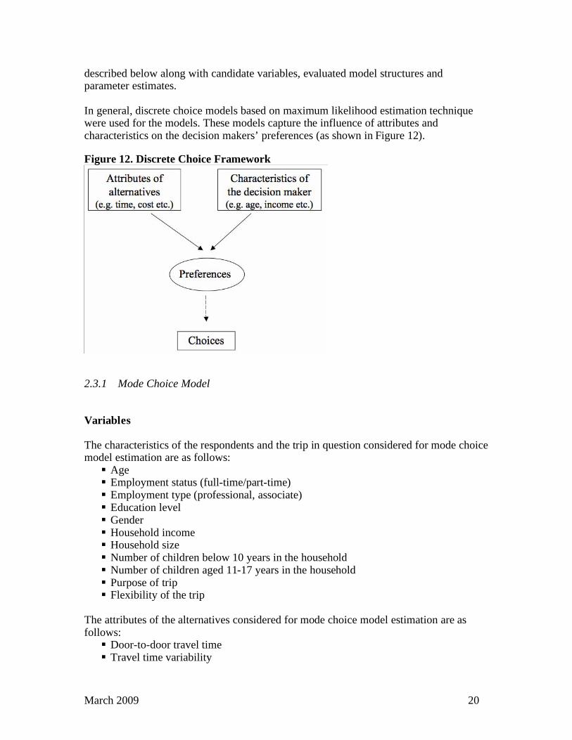
2.2.5 Departure Time Choice Data
In terms of departure time choice, there were a total of 71 observations of respondents who had flexibility in trip scheduling. We assume that departure time after 19:00 pm not available for the trips with purpose of commuting to work or commuting with intermediate stop, and that departure time before 7:00 am and between 7:00-8:00 am are not available for the trips with purpose of returning home or returning home with intermediate stop. Figure 10 and Figure 11 present the distribution of departure time for the selected RP trips and for the SP choice respectively. The number of SP trips departing during 7:00-8:00 pm was larger than that of RP trips, which conflicted with the purpose of peak spreading of congestion pricing. This was carefully reviewed while updating the survey.
March 2009 19
Figure 10. Distribution of Departure Time for the Selected RP Trips
Figure 11. Distribution of Departure Time for the SP Choice
2.3 Model Estimation
Mode choice and departure choice models were estimated separately for the pilot data. Different model specifications were compared in this regard. Each group of models is
March 2009 20
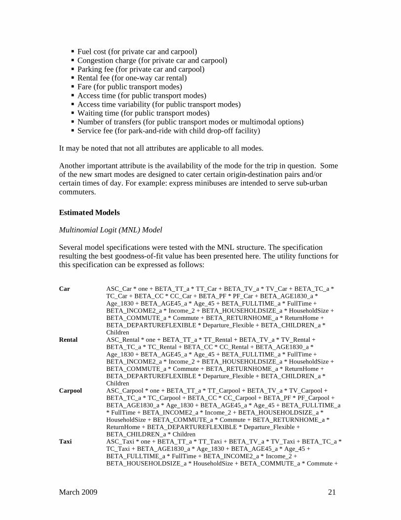
described below along with candidate variables, evaluated model structures and parameter estimates. In general, discrete choice models based on maximum likelihood estimation technique were used for the models. These models capture the influence of attributes and characteristics on the decision makers’ preferences (as shown in Figure 12).
Figure 12. Discrete Choice Framework
2.3.1 Mode Choice Model
Variables The characteristics of the respondents and the trip in question considered for mode choice model estimation are as follows:
! Age ! Employment status (full-time/part-time) ! Employment type (professional, associate) ! Education level ! Gender ! Household income ! Household size ! Number of children below 10 years in the household ! Number of children aged 11-17 years in the household ! Purpose of trip ! Flexibility of the trip
The attributes of the alternatives considered for mode choice model estimation are as follows:
! Door-to-door travel time ! Travel time variability
March 2009 21
! Fuel cost (for private car and carpool) ! Congestion charge (for private car and carpool) ! Parking fee (for private car and carpool) ! Rental fee (for one-way car rental) ! Fare (for public transport modes) ! Access time (for public transport modes) ! Access time variability (for public transport modes) ! Waiting time (for public transport modes) ! Number of transfers (for public transport modes or multimodal options) ! Service fee (for park-and-ride with child drop-off facility)
It may be noted that not all attributes are applicable to all modes. Another important attribute is the availability of the mode for the trip in question. Some of the new smart modes are designed to cater certain origin-destination pairs and/or certain times of day. For example: express minibuses are intended to serve sub-urban commuters.
Estimated Models Multinomial Logit (MNL) Model Several model specifications were tested with the MNL structure. The specification resulting the best goodness-of-fit value has been presented here. The utility functions for this specification can be expressed as follows: Car ASC_Car * one + BETA_TT_a * TT_Car + BETA_TV_a * TV_Car + BETA_TC_a *
TC_Car + BETA_CC * CC_Car + BETA_PF * PF_Car + BETA_AGE1830_a *
Age_1830 + BETA_AGE45_a * Age_45 + BETA_FULLTIME_a * FullTime + BETA_INCOME2_a * Income_2 + BETA_HOUSEHOLDSIZE_a * HouseholdSize + BETA_COMMUTE_a * Commute + BETA_RETURNHOME_a * ReturnHome + BETA_DEPARTUREFLEXIBLE * Departure_Flexible + BETA_CHILDREN_a * Children
Rental ASC_Rental * one + BETA_TT_a * TT_Rental + BETA_TV_a * TV_Rental + BETA_TC_a * TC_Rental + BETA_CC * CC_Rental + BETA_AGE1830_a *
Age_1830 + BETA_AGE45_a * Age_45 + BETA_FULLTIME_a * FullTime + BETA_INCOME2_a * Income_2 + BETA_HOUSEHOLDSIZE_a * HouseholdSize + BETA_COMMUTE_a * Commute + BETA_RETURNHOME_a * ReturnHome + BETA_DEPARTUREFLEXIBLE * Departure_Flexible + BETA_CHILDREN_a * Children
Carpool ASC_Carpool * one + BETA_TT_a * TT_Carpool + BETA_TV_a * TV_Carpool + BETA_TC_a * TC_Carpool + BETA_CC * CC_Carpool + BETA_PF * PF_Carpool +
BETA_AGE1830_a * Age_1830 + BETA_AGE45_a * Age_45 + BETA_FULLTIME_a * FullTime + BETA_INCOME2_a * Income_2 + BETA_HOUSEHOLDSIZE_a * HouseholdSize + BETA_COMMUTE_a * Commute + BETA_RETURNHOME_a * ReturnHome + BETA_DEPARTUREFLEXIBLE * Departure_Flexible + BETA_CHILDREN_a * Children
Taxi ASC_Taxi * one + BETA_TT_a * TT_Taxi + BETA_TV_a * TV_Taxi + BETA_TC_a * TC_Taxi + BETA_AGE1830_a * Age_1830 + BETA_AGE45_a * Age_45 +
BETA_FULLTIME_a * FullTime + BETA_INCOME2_a * Income_2 + BETA_HOUSEHOLDSIZE_a * HouseholdSize + BETA_COMMUTE_a * Commute +
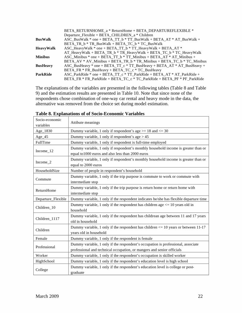
March 2009 22
BETA_RETURNHOME_a * ReturnHome + BETA_DEPARTUREFLEXIBLE * Departure_Flexible + BETA_CHILDREN_a * Children
BusWalk ASC_BusWalk * one + BETA_TT_b * TT_BusWalk + BETA_AT * AT_BusWalk + BETA_TR_b * TR_BusWalk + BETA_TC_b * TC_BusWalk
HeavyWalk ASC_HeavyWalk * one + BETA_TT_b * TT_HeavyWalk + BETA_AT * AT_HeavyWalk + BETA_TR_b * TR_HeavyWalk + BETA_TC_b * TC_HeavyWalk
Minibus ASC_Minibus * one + BETA_TT_b * TT_Minibus + BETA_AT * AT_Minibus + BETA_AV * AV_Minibus + BETA_TR_b * TR_Minibus + BETA_TC_b * TC_Minibus
BusHeavy ASC_BusHeavy * one + BETA_TT_c * TT_BusHeavy + BETA_AT * AT_BusHeavy + BETA_FR * FR_BusHeavy + BETA_TC_c * TC_BusHeavy
ParkRide ASC_ParkRide * one + BETA_TT_c * TT_ParkRide + BETA_AT * AT_ParkRide +
BETA_FR * FR_ParkRide + BETA_TC_c * TC_ParkRide + BETA_PF * PF_ParkRide
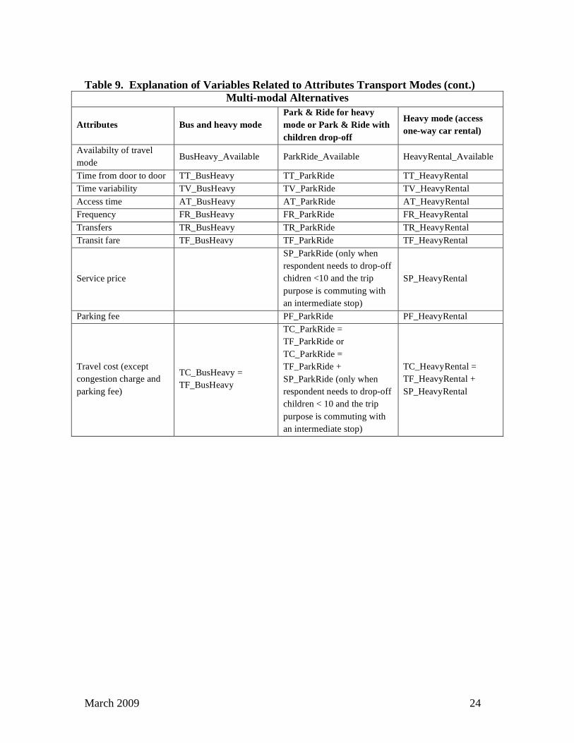
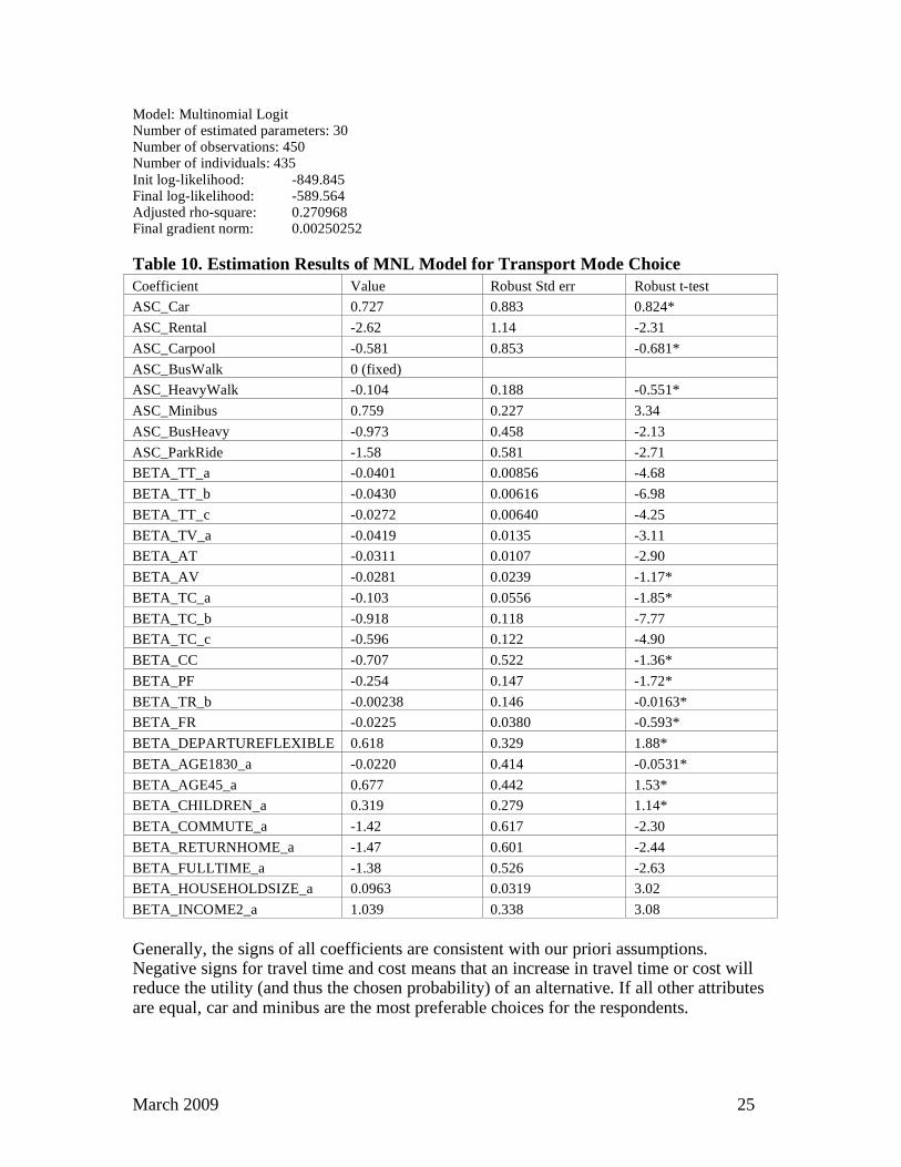
The explanations of the variables are presented in the following tables (Table 8 and Table 9) and the estimation results are presented in Table 10. Note that since none of the respondents chose combination of one-way car rental and heavy mode in the data, the alternative was removed from the choice set during model estimation.
Table 8. Explanations of of Socio-Economic Variables
Socio-economic
variables Attibute meanings
Age_1830 Dummy variable, 1 only if respondent’s age >= 18 and <= 30
Age_45 Dummy variable, 1 only if respondent’s age > 45
FullTime Dummy variable, 1 only if respondent is full-time employed
Income_12 Dummy variable, 1 only if respondent’s monthly household income is greater than or
equal to1000 euros and also less than 2000 euros
Income_2 Dummy variable, 1 only if respondent’s monthly household income is greater than or
equal to 2000 euros
HouseholdSize Number of people in respondent’s household
Commute Dummy variable, 1 only if the trip purpose is commute to work or commute with
intermediate stop
ReturnHome Dummy variable, 1 only if the trip purpose is return home or return home with
intermediate stop
Departure_Flexible Dummy variable, 1 only if the respondent indicates he/she has flexible departure time
Children_10 Dummy variable, 1 only if the respondent has children age <= 10 years old in
household
Children_1117 Dummy variable, 1 only if the respondent has childrean age between 11 and 17 years
old in household
Children Dummy variable, 1 only if the respondent has children <= 10 years or between 11-17
years old in household
Female Dummy variable, 1 only if the respondent is female
Professional Dummy variable, 1 only if the respondent’s occupation is professional, associate
professional and technical occupation, or mangers and senior officials
Worker Dummy variable, 1 only if the respondent’s occupation is skilled worker
HighSchool Dummy variable, 1 only if the respondent’s education level is high school
College Dummy variable, 1 only if the respondent’s education level is college or post-
graduate
March 2009 23
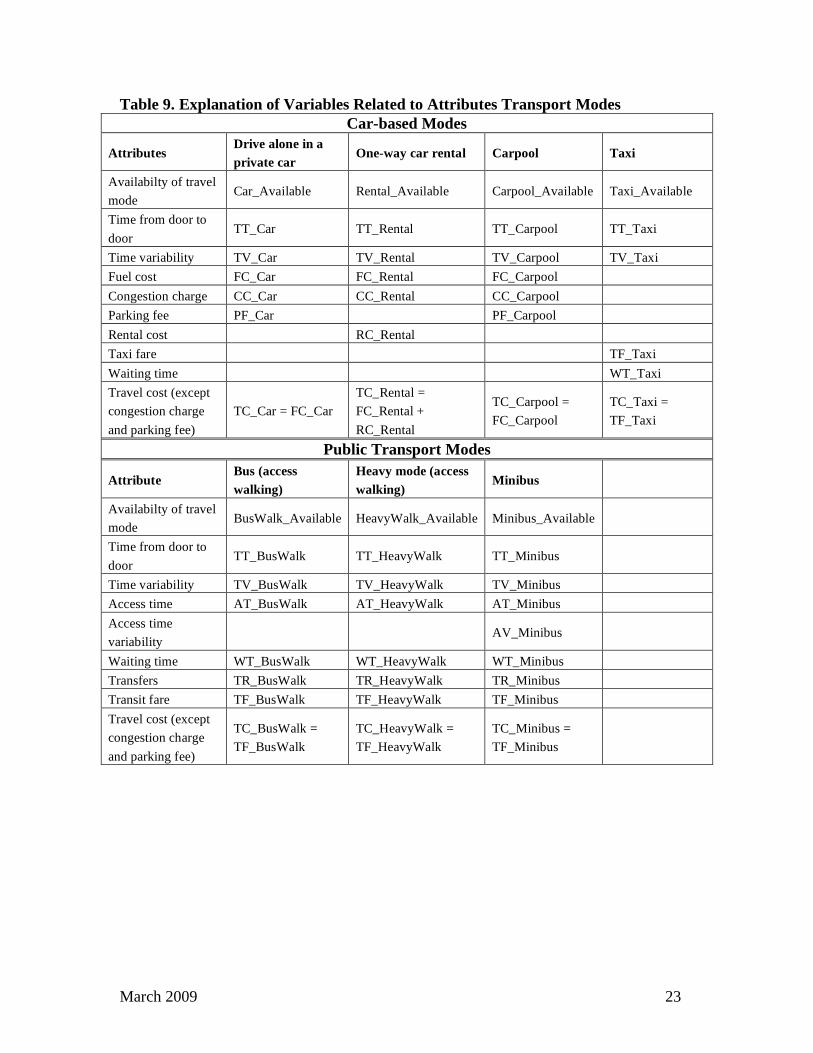
Table 9. Explanation of Variables Related to Attributes Transport Modes
Car-based Modes
Attributes Drive alone in a
private car One-way car rental Carpool Taxi
Availabilty of travel
mode Car_Available Rental_Available Carpool_Available Taxi_Available
Time from door to
door TT_Car TT_Rental TT_Carpool TT_Taxi
Time variability TV_Car TV_Rental TV_Carpool TV_Taxi
Fuel cost FC_Car FC_Rental FC_Carpool
Congestion charge CC_Car CC_Rental CC_Carpool
Parking fee PF_Car PF_Carpool
Rental cost RC_Rental
Taxi fare TF_Taxi
Waiting time WT_Taxi
Travel cost (except
congestion charge
and parking fee)
TC_Car = FC_Car
TC_Rental =
FC_Rental +
RC_Rental
TC_Carpool =
FC_Carpool
TC_Taxi =
TF_Taxi
Public Transport Modes
Attribute Bus (access
walking)
Heavy mode (access
walking) Minibus
Availabilty of travel
mode BusWalk_Available HeavyWalk_Available Minibus_Available
Time from door to
door TT_BusWalk TT_HeavyWalk TT_Minibus
Time variability TV_BusWalk TV_HeavyWalk TV_Minibus
Access time AT_BusWalk AT_HeavyWalk AT_Minibus
Access time
variability AV_Minibus
Waiting time WT_BusWalk WT_HeavyWalk WT_Minibus
Transfers TR_BusWalk TR_HeavyWalk TR_Minibus
Transit fare TF_BusWalk TF_HeavyWalk TF_Minibus
Travel cost (except
congestion charge
and parking fee)
TC_BusWalk =
TF_BusWalk
TC_HeavyWalk =
TF_HeavyWalk
TC_Minibus =
TF_Minibus
March 2009 24
Table 9. Explanation of Variables Related to Attributes Transport Modes (cont.)
Multi-modal Alternatives
Attributes Bus and heavy mode
Park & Ride for heavy
mode or Park & Ride with
children drop-off
Heavy mode (access
one-way car rental)
Availabilty of travel
mode BusHeavy_Available ParkRide_Available HeavyRental_Available
Time from door to door TT_BusHeavy TT_ParkRide TT_HeavyRental
Time variability TV_BusHeavy TV_ParkRide TV_HeavyRental
Access time AT_BusHeavy AT_ParkRide AT_HeavyRental
Frequency FR_BusHeavy FR_ParkRide FR_HeavyRental
Transfers TR_BusHeavy TR_ParkRide TR_HeavyRental
Transit fare TF_BusHeavy TF_ParkRide TF_HeavyRental
Service price
SP_ParkRide (only when
respondent needs to drop-off
chidren <10 and the trip
purpose is commuting with
an intermediate stop)
SP_HeavyRental
Parking fee PF_ParkRide PF_HeavyRental
Travel cost (except
congestion charge and
parking fee)
TC_BusHeavy =
TF_BusHeavy
TC_ParkRide =
TF_ParkRide or
TC_ParkRide =
TF_ParkRide +
SP_ParkRide (only when
respondent needs to drop-off
children < 10 and the trip
purpose is commuting with
an intermediate stop)
TC_HeavyRental =
TF_HeavyRental +
SP_HeavyRental
March 2009 25
Model: Multinomial Logit Number of estimated parameters: 30 Number of observations: 450 Number of individuals: 435
Init log-likelihood: -849.845 Final log-likelihood: -589.564 Adjusted rho-square: 0.270968 Final gradient norm: 0.00250252
Table 10. Estimation Results of MNL Model for Transport Mode Choice
Coefficient Value Robust Std err Robust t-test
ASC_Car 0.727 0.883 0.824*
ASC_Rental -2.62 1.14 -2.31
ASC_Carpool -0.581 0.853 -0.681*
ASC_BusWalk 0 (fixed)
ASC_HeavyWalk -0.104 0.188 -0.551*
ASC_Minibus 0.759 0.227 3.34
ASC_BusHeavy -0.973 0.458 -2.13
ASC_ParkRide -1.58 0.581 -2.71
BETA_TT_a -0.0401 0.00856 -4.68
BETA_TT_b -0.0430 0.00616 -6.98
BETA_TT_c -0.0272 0.00640 -4.25
BETA_TV_a -0.0419 0.0135 -3.11
BETA_AT -0.0311 0.0107 -2.90
BETA_AV -0.0281 0.0239 -1.17*
BETA_TC_a -0.103 0.0556 -1.85*
BETA_TC_b -0.918 0.118 -7.77
BETA_TC_c -0.596 0.122 -4.90
BETA_CC -0.707 0.522 -1.36*
BETA_PF -0.254 0.147 -1.72*
BETA_TR_b -0.00238 0.146 -0.0163*
BETA_FR -0.0225 0.0380 -0.593*
BETA_DEPARTUREFLEXIBLE 0.618 0.329 1.88*
BETA_AGE1830_a -0.0220 0.414 -0.0531*
BETA_AGE45_a 0.677 0.442 1.53*
BETA_CHILDREN_a 0.319 0.279 1.14*
BETA_COMMUTE_a -1.42 0.617 -2.30
BETA_RETURNHOME_a -1.47 0.601 -2.44
BETA_FULLTIME_a -1.38 0.526 -2.63
BETA_HOUSEHOLDSIZE_a 0.0963 0.0319 3.02
BETA_INCOME2_a 1.039 0.338 3.08
Generally, the signs of all coefficients are consistent with our priori assumptions. Negative signs for travel time and cost means that an increase in travel time or cost will reduce the utility (and thus the chosen probability) of an alternative. If all other attributes are equal, car and minibus are the most preferable choices for the respondents.
March 2009 26
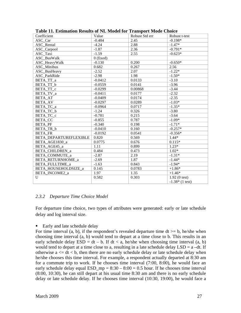
The travel time variability emerges as a significant attribute for car-related modes. This is because cars are highly sensible to traffic congestion. Accurate predications of travel time with information services would increase car use. For car-related modes, the sensitivities to different forms of cost were found to be as follows: congestion charge > parking fee > travel cost This indicates that introducing the congestion charge and increasing the parking price is likely to have a greater impact in deterring car usage compared to increasing the general travel cost (e.g. fuel cost, rental cost etc.). Dummy variable of departure time flexibility is has positive coefficient, therefore people who prefer flexibility is more likely to choose car-related modes. Waiting time is not a well-defined attribute for public transportation compared with frequency, and its coefficient is insignificant. The number of transfers is also insignificant. These were noted in updating the main survey. Significant socio-economic variables include the age of the respondent, number of children in the respondents' household, trip purpose, employment status, household size, and monthly household income. Nested Logit (NL) Model Nested Logit (NL) models were also applied for transport mode choice, assuming there were three nests for transport modes: car-based nest (drive alone in private car, one-way car rental, carpool, shared taxi), public transportation nest (bus, heavy mode, minibus), and multi-modal nest (bus and heavy mode, park & ride with child drop-off, one-way car rental with heavy mode). The best model specification was same as that of the selected MNL model. The estimation results of the NL model are shown in Table 11. Firstly, the coefficients of the three nests were set to one. The top coefficient for the NL structure was estimated with u = 0.58, which was different from zero or one. The conclusions are similar to those of the selected MNL model. The main differences are that the constant of ASC_car is negative and the sign of the coefficient for respondents aged between 18 and 30 is positive in the NL model. Model: Nested Logit
Number of estimated parameters: 31 Number of observations: 450 Number of individuals: 435 Init log-likelihood: -849.845 Final log-likelihood: -586.408 Adjusted rho-square: 0.273506 Final gradient norm: 0.00412607
March 2009 27
Table 11. Estimation Results of NL Model for Transport Mode Choice Coefficient Value Robust Std err Robust t-test
ASC_Car -0.484 2.45 -0.198* ASC_Rental -4.24 2.88 -1.47*
ASC_Carpool -1.87 2.36 -0.791*
ASC_Taxi -1.59 2.55 -0.623* ASC_BusWalk 0 (fixed)
ASC_HeavyWalk -0.130 0.200 -0.650* ASC_Minibus 0.682 0.267 2.56
ASC_BusHeavy -2.52 2.07 -1.22* ASC_ParkRide -2.98 1.98 -1.50*
BETA_TT_a -0.0412 0.0133 -3.10
BETA_TT_b -0.0559 0.0141 -3.96 BETA_TT_c -0.0299 0.00868 -3.44
BETA_TV_a -0.0411 0.0177 -2.32 BETA_AT -0.0409 0.0174 -2.35
BETA_AV -0.0297 0.0289 -1.03* BETA_TC_a -0.0964 0.0717 -1.35*
BETA_TC_b -1.24 0.326 -3.80 BETA_TC_c -0.781 0.215 -3.64
BETA_CC -0.855 0.787 -1.09*
BETA_PF -0.340 0.198 -1.71* BETA_TR_b -0.0410 0.160 -0.257*
BETA_FR -0.0192 0.0541 -0.356* BETA_DEPARTUREFLEXIBLE 0.820 0.569 1.44*
BETA_AGE1830_a 0.0775 0.676 0.115* BETA_AGE45_a 1.11 0.899 1.23*
BETA_CHILDREN_a 0.484 0.473 1.02*
BETA_COMMUTE_a -2.87 2.19 -1.31* BETA_RETURNHOME_a -2.69 1.87 -1.44*
BETA_FULLTIME_a -1.63 0.843 -1.94* BETA_HOUSEHOLDSIZE_a 0.145 0.0783 +1.86*
BETA_INCOME2_a 1.97 1.35 +1.46* U 0.582 0.303 1.92 (0 test)
-1.38* (1 test)
2.3.2 Departure Time Choice Model
For departure time choice, two types of attributes were generated: early or late schedule
delay and log interval size.
! Early and late schedule delay For time interval (a, b), if the respondent’s revealed departure time dt >= b, he/she when choosing time interval (a, b) would tend to depart at a time close to b. This results in an early schedule delay ESD = dt – b. If dt < a, he/she when choosing time interval (a, b) would tend to depart at a time close to a, resulting in a late schedule delay LSD = a –dt. If otherwise a <= dt < b, then there are no early schedule delay or late schedule delay when he/she chooses this time interval. For example, a respondent actually departed at 8:30 am for a commute trip to work. If he chooses time interval (7:00, 8:00), he would face an early schedule delay equal ESD_mp = 8:30 – 8:00 = 0.5 hour. If he chooses time interval (8:00, 10:30), he can still depart at his usual time 8:30 am and there is no early schedule delay or late schedule delay. If he chooses time interval (10:30, 19:00), he would face a
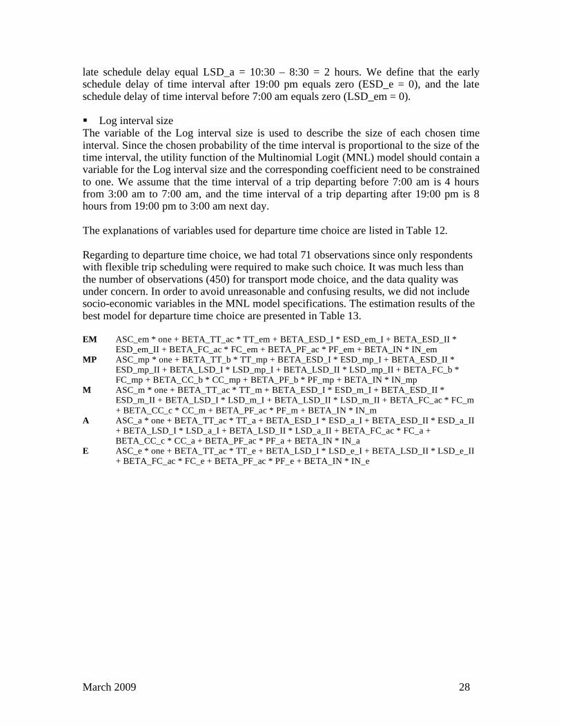
March 2009 28
late schedule delay equal LSD_a = 10:30 – 8:30 = 2 hours. We define that the early schedule delay of time interval after 19:00 pm equals zero (ESD_e = 0), and the late schedule delay of time interval before 7:00 am equals zero (LSD_em = 0). ! Log interval size The variable of the Log interval size is used to describe the size of each chosen time interval. Since the chosen probability of the time interval is proportional to the size of the time interval, the utility function of the Multinomial Logit (MNL) model should contain a variable for the Log interval size and the corresponding coefficient need to be constrained to one. We assume that the time interval of a trip departing before 7:00 am is 4 hours from 3:00 am to 7:00 am, and the time interval of a trip departing after 19:00 pm is 8 hours from 19:00 pm to 3:00 am next day. The explanations of variables used for departure time choice are listed in Table 12. Regarding to departure time choice, we had total 71 observations since only respondents with flexible trip scheduling were required to make such choice. It was much less than the number of observations (450) for transport mode choice, and the data quality was under concern. In order to avoid unreasonable and confusing results, we did not include socio-economic variables in the MNL model specifications. The estimation results of the best model for departure time choice are presented in Table 13. EM ASC_em * one + BETA_TT_ac * TT_em + BETA_ESD_I * ESD_em_I + BETA_ESD_II *
ESD_em_II + BETA_FC_ac * FC_em + BETA_PF_ac * PF_em + BETA_IN * IN_em MP ASC_mp * one + BETA_TT_b * TT_mp + BETA_ESD_I * ESD_mp_I + BETA_ESD_II *
ESD_mp_II + BETA_LSD_I * LSD_mp_I + BETA_LSD_II * LSD_mp_II + BETA_FC_b * FC_mp + BETA_CC_b * CC_mp + BETA_PF_b * PF_mp + BETA_IN * IN_mp
M ASC_m * one + BETA_TT_ac * TT_m + BETA_ESD_I * ESD_m_I + BETA_ESD_II * ESD_m_II + BETA_LSD_I * LSD_m_I + BETA_LSD_II * LSD_m_II + BETA_FC_ac * FC_m
+ BETA_CC_c * CC_m + BETA_PF_ac * PF_m + BETA_IN * IN_m A ASC_a * one + BETA_TT_ac * TT_a + BETA_ESD_I * ESD_a_I + BETA_ESD_II * ESD_a_II
+ BETA_LSD_I * LSD_a_I + BETA_LSD_II * LSD_a_II + BETA_FC_ac * FC_a + BETA_CC_c * CC_a + BETA_PF_ac * PF_a + BETA_IN * IN_a
E ASC_e * one + BETA_TT_ac * TT_e + BETA_LSD_I * LSD_e_I + BETA_LSD_II * LSD_e_II + BETA_FC_ac * FC_e + BETA_PF_ac * PF_e + BETA_IN * IN_e
March 2009 29
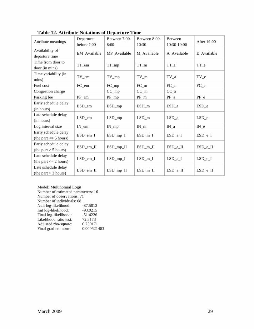
Table 12. Attribute Notations of Departure Time
Attribute meanings Departure
before 7:00
Between 7:00-
8:00
Between 8:00-
10:30
Between
10:30-19:00 After 19:00
Availability of
departure time EM_Available MP_Available M_Available A_Available E_Available
Time from door to
door (in mins) TT_em TT_mp TT_m TT_a TT_e
Time variability (in
mins) TV_em TV_mp TV_m TV_a TV_e
Fuel cost FC_em FC_mp FC_m FC_a FC_e
Congestion charge CC_mp CC_m CC_a
Parking fee PF_em PF_mp PF_m PF_a PF_e
Early schedule delay
(in hours) ESD_em ESD_mp ESD_m ESD_a ESD_e
Late schedule delay
(in hours) LSD_em LSD_mp LSD_m LSD_a LSD_e
Log interval size IN_em IN_mp IN_m IN_a IN_e
Early schedule delay
(the part <= 5 hours) ESD_em_I ESD_mp_I ESD_m_I ESD_a_I ESD_e_I
Early schedule delay
(the part > 5 hours) ESD_em_II ESD_mp_II ESD_m_II ESD_a_II ESD_e_II
Late schedule delay
(the part <= 2 hours) LSD_em_I LSD_mp_I LSD_m_I LSD_a_I LSD_e_I
Late schedule delay
(the part > 2 hours) LSD_em_II LSD_mp_II LSD_m_II LSD_a_II LSD_e_II
Model: Multinomial Logit Number of estimated parameters: 16 Number of observations: 71 Number of individuals: 68 Null log-likelihood: -87.5813
Init log-likelihood: -93.0215 Final log-likelihood: -51.4226 Likelihood ratio test: 72.3173 Adjusted rho-square: 0.230171 Final gradient norm: 0.000521483
March 2009 30
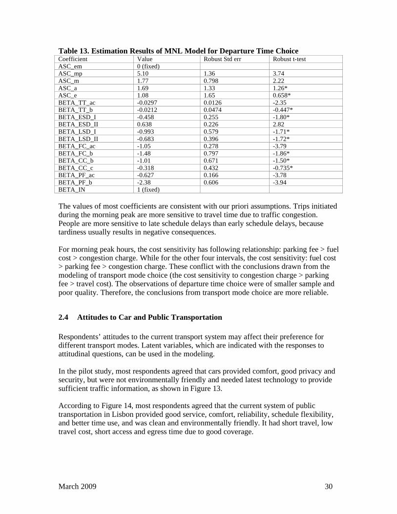
Table 13. Estimation Results of MNL Model for Departure Time Choice Coefficient Value Robust Std err Robust t-test
ASC_em 0 (fixed) ASC_mp 5.10 1.36 3.74
ASC_m 1.77 0.798 2.22
ASC_a 1.69 1.33 1.26* ASC_e 1.08 1.65 0.658*
BETA_TT_ac -0.0297 0.0126 -2.35 BETA_TT_b -0.0212 0.0474 -0.447*
BETA_ESD_I -0.458 0.255 -1.80* BETA_ESD_II 0.638 0.226 2.82
BETA_LSD_I -0.993 0.579 -1.71*
BETA_LSD_II -0.683 0.396 -1.72* BETA_FC_ac -1.05 0.278 -3.79
BETA_FC_b -1.48 0.797 -1.86* BETA_CC_b -1.01 0.671 -1.50*
BETA_CC_c -0.318 0.432 -0.735* BETA_PF_ac -0.627 0.166 -3.78
BETA_PF_b -2.38 0.606 -3.94 BETA_IN 1 (fixed)
The values of most coefficients are consistent with our priori assumptions. Trips initiated during the morning peak are more sensitive to travel time due to traffic congestion. People are more sensitive to late schedule delays than early schedule delays, because tardiness usually results in negative consequences. For morning peak hours, the cost sensitivity has following relationship: parking fee > fuel cost > congestion charge. While for the other four intervals, the cost sensitivity: fuel cost > parking fee > congestion charge. These conflict with the conclusions drawn from the modeling of transport mode choice (the cost sensitivity to congestion charge > parking fee > travel cost). The observations of departure time choice were of smaller sample and poor quality. Therefore, the conclusions from transport mode choice are more reliable.
2.4 Attitudes to Car and Public Transportation
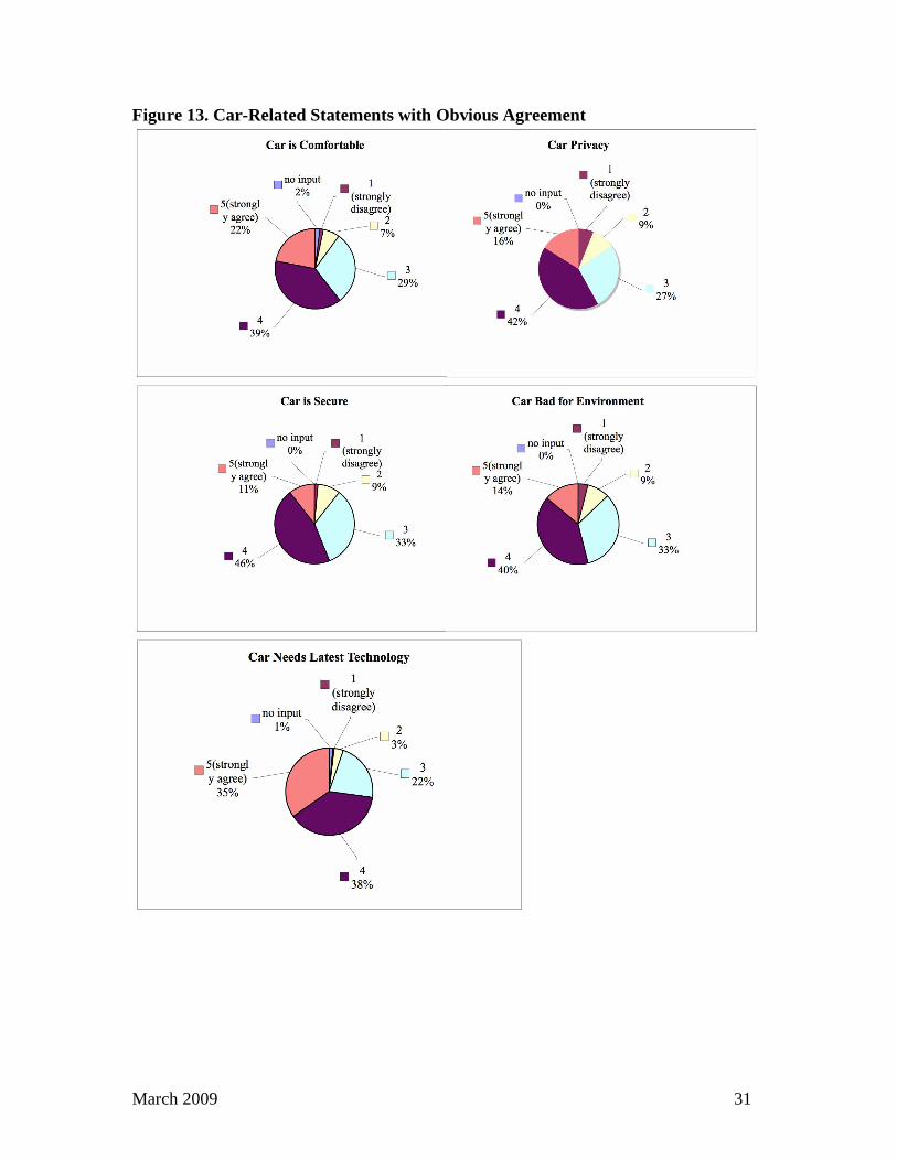
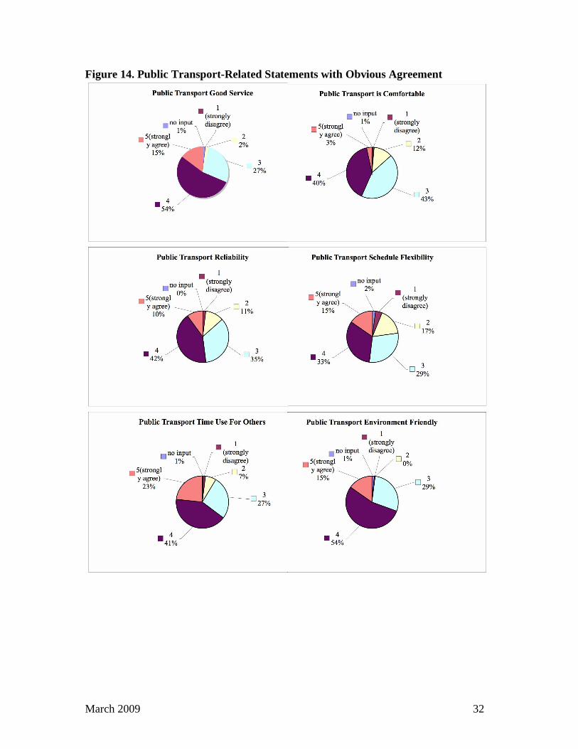
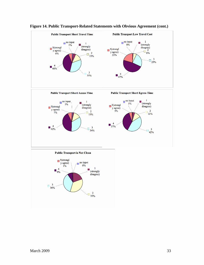
Respondents’ attitudes to the current transport system may affect their preference for different transport modes. Latent variables, which are indicated with the responses to attitudinal questions, can be used in the modeling. In the pilot study, most respondents agreed that cars provided comfort, good privacy and security, but were not environmentally friendly and needed latest technology to provide sufficient traffic information, as shown in Figure 13. According to Figure 14, most respondents agreed that the current system of public transportation in Lisbon provided good service, comfort, reliability, schedule flexibility, and better time use, and was clean and environmentally friendly. It had short travel, low travel cost, short access and egress time due to good coverage.
March 2009 31
Figure 13. Car-Related Statements with Obvious Agreement
March 2009 32
Figure 14. Public Transport-Related Statements with Obvious Agreement
March 2009 33
Figure 14. Public Transport-Related Statements with Obvious Agreement (cont.)
March 2009 34
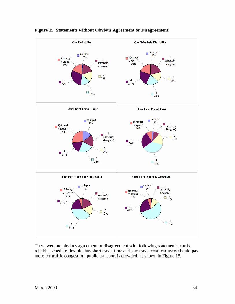
Figure 15. Statements without Obvious Agreement or Disagreement
There were no obvious agreement or disagreement with following statements: car is reliable, schedule flexible, has short travel time and low travel cost; car users should pay more for traffic congestion; public transport is crowded, as shown in Figure 15.
March 2009 35
2.5 Information Services
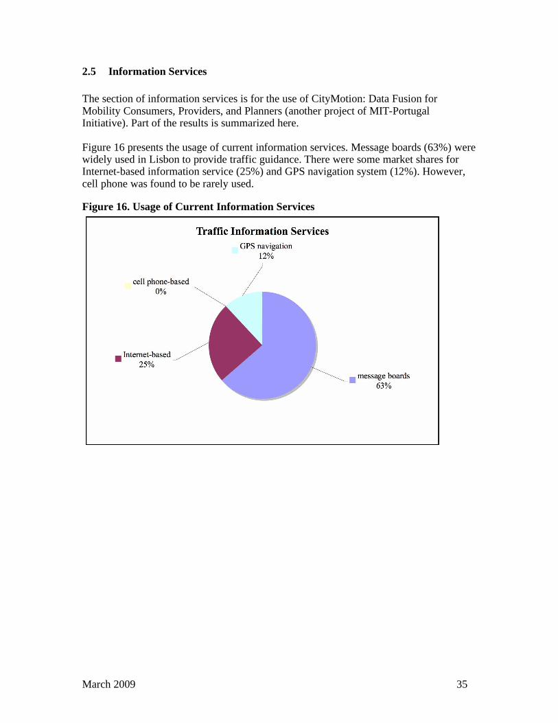
The section of information services is for the use of CityMotion: Data Fusion for Mobility Consumers, Providers, and Planners (another project of MIT-Portugal Initiative). Part of the results is summarized here. Figure 16 presents the usage of current information services. Message boards (63%) were widely used in Lisbon to provide traffic guidance. There were some market shares for Internet-based information service (25%) and GPS navigation system (12%). However, cell phone was found to be rarely used.
Figure 16. Usage of Current Information Services
March 2009 36
3 Revised Stated Preference Survey
3.1 Main Adjustments from Pilot Study
An important objective of pilot study was to test the SP survey structure and the validity of experimental design. According to the estimation results, there were much fewer and lower quality responses to the SP scenarios of departure time choice compared with those to the SP scenarios of travel mode choice; some of the attributes of innovative modes were not found to be as important as expected, e.g., sensitivity to waiting time and number of transfers were insignificant. Furthermore, average survey time was longer than 20 min so that the SP questionnaire needed to be shortened. Substantial changes were made to solve these problems and especially to get a more robust and rich SP survey. The key changes in the survey structure are as follows:
! Integrated the departure time choice with the mode choice exercises to better capture the effect of congestion charge
! Reduced the number of SP scenarios to two ! Eliminated the section on information services from the survey
In addition, the context of SP survey was adjusted as follows:
! Deleted the alternative of carpool but added regular taxi ! Included preferred occupancy as a choice dimension to better represent car
sharing ! Used time-varying attributes, such as travel time, congestion charge, frequency
and access time to better represent the context of departure time choice ! Added new questions and attributes (parking fee and search time for parking
space) in SP scenarios regarding to parking pricing and enforcement ! Added regular fee as an attribute, if freeway was tolled (charged) ! Waiting time replaced by frequency
In Section 3.2, we present the updated SP scenarios. Several changes were made in the experimental design of the survey as well, which are documented in Section 3.3.
3.2 Updated SP Scenarios with Multidimensional Choice
The first dimensional choice of SP scenarios was the mode choice, the second one the departure time choice and the third one occupancy choice (if applicable). In the revised survey, the new travel modes here included shared taxis, express minibus, one-way car rentals, park-and-ride systems with a tutored delivery of children to their schools, and one-way car rentals with heavy mode. Alongside the five existing modes (car, regular taxi, bus, heavy mode, and bus and heavy modes), this yielded a travel mode choice set of up to ten alternatives per respondent. The first dimensional choice of SP scenarios was the choice consisted of these existing and new travel modes. The level-of-service of these alternatives varied substantially on the departure time; in particular there were significantly long travel time and high costs (in the form of
March 2009 37
congestion charge and parking enforcement) for traveling in peak hours. This is expected to strongly influence the individual travel pattern and the choice of departure time intervals was included in the SP survey as a second dimension. In addition, it is expected that these radically different modes and level-of-service are likely to foster the sharing of trips. A third dimension has been added in the choice structure: the choice of occupancy for private car, one-way car rentals and regular taxi.
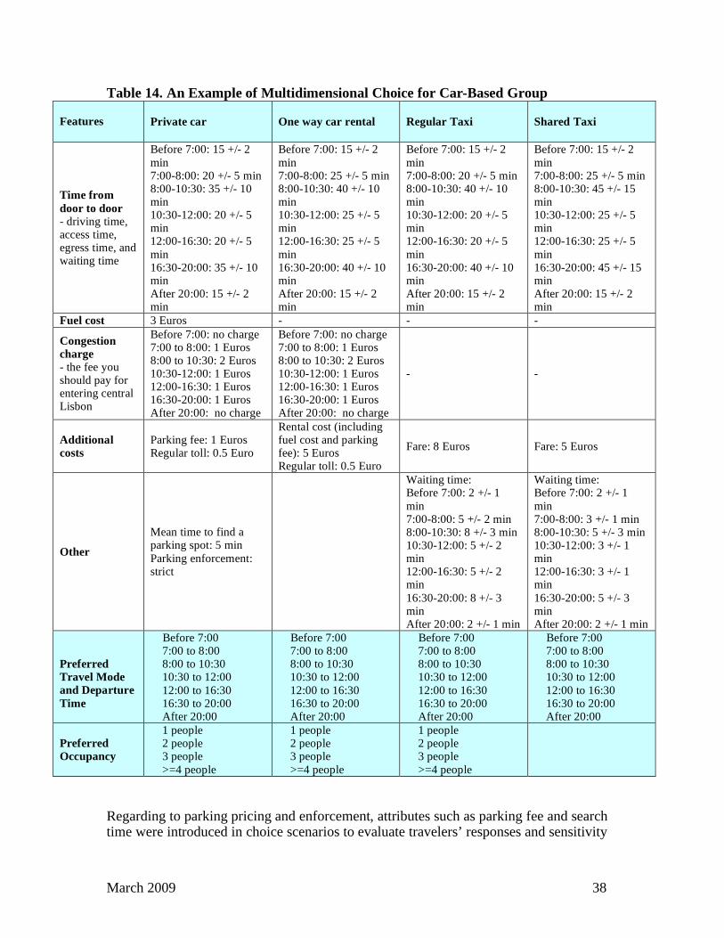
The organization and presentation of a multidimensional choice exercise with such a large number of alternatives and attributes posed a challenge for the revised SP survey, since cognitive burden may force respondents to adopt a simple decision strategy based on only partial information (Caussade et al. 2005). To minimize the complexity, a similar grouping as in the Pilot study was implemented: the alternatives were first presented sequentially in three groups: car-based, public transport based and multi-modal (see Table 14, Table 15 and Table 16). Respondents were asked to choose their ‘preferred’ combinations of mode, departure time and occupancy (if applicable) in each case. The three preferred combinations were then presented in a single choice task and the respondent was asked to select the combination of his ‘choice’. In this organization, each respondent was presented with two SP scenarios, four choice tasks, at most four alternatives per choice task, and at most seven attributes per alternative (see Table 17). For an instance of the multidimensional choice for car-based group (see Table 14), here are the descriptions for some attributes.
! The time from door to door includes the time spent to reach the car/taxi, the actual driving time, the time spent to reach the final destination after getting out of the car/taxi, and the waiting time (especially for shared taxi). This time may vary from day to day depending on traffic conditions. The +/- sign in the time represents this variability. The time may be more predictable (less variation) if real-time travel information is available.
! The fuel cost, congestion charge, parking fee, regular toll and other costs are the total amount of out-of-pocket costs for your trip, regardless of whether or not you share the expenses with household members, co-workers, neighbors or others. We assume that if respondents receive reimbursement for toll/parking, that these reimbursements are still valid.
! The travel time, congestion charge, and waiting time of shared taxi may vary depending on the departure time and is the highest during peak periods. Peak periods are 8:00 to 10:30 in the morning and 16:30 to 20:00 in the afternoon.
! Mean time to find a parking spot is the time used to search for an available parking spot near your final destination. If parking enforcement is strict, it means when you park illegally you will certainly be fined or your car will be towed.
! Preferred occupancy refers to the possible total number of people among whom the costs will be shared (either formally or informally). Respondents are not required to choose preferred occupancy for shared taxi, since the respondents cannot predict how many people will share the taxi.
March 2009 38
Table 14. An Example of Multidimensional Choice for Car-Based Group
Features
Private car One way car rental Regular Taxi Shared Taxi
Time from
door to door
- driving time, access time, egress time, and waiting time
Before 7:00: 15 +/- 2
min 7:00-8:00: 20 +/- 5 min 8:00-10:30: 35 +/- 10 min 10:30-12:00: 20 +/- 5 min 12:00-16:30: 20 +/- 5
min 16:30-20:00: 35 +/- 10 min After 20:00: 15 +/- 2 min
Before 7:00: 15 +/- 2
min 7:00-8:00: 25 +/- 5 min 8:00-10:30: 40 +/- 10 min 10:30-12:00: 25 +/- 5 min 12:00-16:30: 25 +/- 5
min 16:30-20:00: 40 +/- 10 min After 20:00: 15 +/- 2 min
Before 7:00: 15 +/- 2
min 7:00-8:00: 20 +/- 5 min 8:00-10:30: 40 +/- 10 min 10:30-12:00: 20 +/- 5 min 12:00-16:30: 20 +/- 5
min 16:30-20:00: 40 +/- 10 min After 20:00: 15 +/- 2 min
Before 7:00: 15 +/- 2
min 7:00-8:00: 25 +/- 5 min 8:00-10:30: 45 +/- 15 min 10:30-12:00: 25 +/- 5 min 12:00-16:30: 25 +/- 5
min 16:30-20:00: 45 +/- 15 min After 20:00: 15 +/- 2 min
Fuel cost 3 Euros - - -
Congestion
charge
- the fee you should pay for entering central Lisbon
Before 7:00: no charge 7:00 to 8:00: 1 Euros 8:00 to 10:30: 2 Euros 10:30-12:00: 1 Euros 12:00-16:30: 1 Euros 16:30-20:00: 1 Euros After 20:00: no charge
Before 7:00: no charge 7:00 to 8:00: 1 Euros 8:00 to 10:30: 2 Euros 10:30-12:00: 1 Euros 12:00-16:30: 1 Euros 16:30-20:00: 1 Euros After 20:00: no charge
- -
Additional
costs
Parking fee: 1 Euros Regular toll: 0.5 Euro
Rental cost (including fuel cost and parking fee): 5 Euros Regular toll: 0.5 Euro
Fare: 8 Euros Fare: 5 Euros
Other
Mean time to find a parking spot: 5 min
Parking enforcement: strict
Waiting time: Before 7:00: 2 +/- 1
min 7:00-8:00: 5 +/- 2 min 8:00-10:30: 8 +/- 3 min 10:30-12:00: 5 +/- 2 min 12:00-16:30: 5 +/- 2 min
16:30-20:00: 8 +/- 3 min After 20:00: 2 +/- 1 min
Waiting time: Before 7:00: 2 +/- 1
min 7:00-8:00: 3 +/- 1 min 8:00-10:30: 5 +/- 3 min 10:30-12:00: 3 +/- 1 min 12:00-16:30: 3 +/- 1 min
16:30-20:00: 5 +/- 3 min After 20:00: 2 +/- 1 min
Preferred
Travel Mode
and Departure
Time
Before 7:00 7:00 to 8:00 8:00 to 10:30 10:30 to 12:00
12:00 to 16:30 16:30 to 20:00 After 20:00
Before 7:00 7:00 to 8:00 8:00 to 10:30 10:30 to 12:00
12:00 to 16:30 16:30 to 20:00 After 20:00
Before 7:00 7:00 to 8:00 8:00 to 10:30 10:30 to 12:00
12:00 to 16:30 16:30 to 20:00 After 20:00
Before 7:00 7:00 to 8:00 8:00 to 10:30 10:30 to 12:00
12:00 to 16:30 16:30 to 20:00 After 20:00
Preferred
Occupancy
1 people 2 people 3 people
>=4 people
1 people 2 people 3 people
>=4 people
1 people 2 people 3 people
>=4 people
Regarding to parking pricing and enforcement, attributes such as parking fee and search time were introduced in choice scenarios to evaluate travelers’ responses and sensitivity
March 2009 39
(see Hensher and King 2001, Alberta and Mahalel 2006). In addition, travelers were asked about their perception of parking conditions at/near trip destinations and their personal attitudes to parking problems as follows. Which of the following are applicable to parking facilities at/near your destination (select all that are applicable):
Parking is fully free on the street There are some paid and some free parking spots on the street There are dedicated parking lots Parking is strongly and effectively enforced It is easy to find a parking spot
Please indicate your level of agreement with the following statements (rank from 1 strongly disagree to 5 strongly agree).
Difficulty in getting a parking spot near the destination is the main problem of using the car. Parking illegally is a major offence. High parking cost is a major problem of using the car.
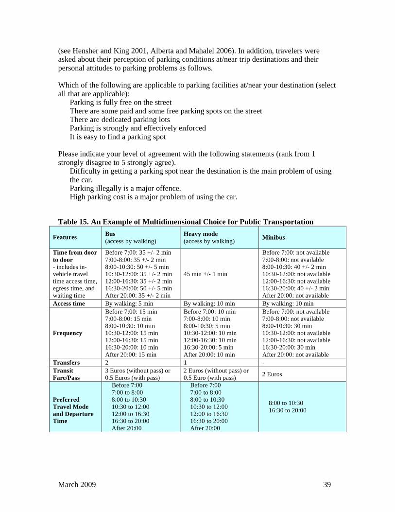
Table 15. An Example of Multidimensional Choice for Public Transportation
Features
Bus
(access by walking)
Heavy mode
(access by walking) Minibus
Time from door
to door
- includes in-vehicle travel time access time, egress time, and waiting time
Before 7:00: 35 +/- 2 min
7:00-8:00: 35 +/- 2 min 8:00-10:30: 50 +/- 5 min 10:30-12:00: 35 +/- 2 min 12:00-16:30: 35 +/- 2 min 16:30-20:00: 50 +/- 5 min After 20:00: 35 +/- 2 min
45 min +/- 1 min
Before 7:00: not available
7:00-8:00: not available 8:00-10:30: 40 +/- 2 min 10:30-12:00: not available 12:00-16:30: not available 16:30-20:00: 40 +/- 2 min After 20:00: not available
Access time By walking: 5 min By walking: 10 min By walking: 10 min
Frequency
Before 7:00: 15 min 7:00-8:00: 15 min 8:00-10:30: 10 min 10:30-12:00: 15 min 12:00-16:30: 15 min 16:30-20:00: 10 min
After 20:00: 15 min
Before 7:00: 10 min 7:00-8:00: 10 min 8:00-10:30: 5 min 10:30-12:00: 10 min 12:00-16:30: 10 min 16:30-20:00: 5 min
After 20:00: 10 min
Before 7:00: not available 7:00-8:00: not available 8:00-10:30: 30 min 10:30-12:00: not available 12:00-16:30: not available 16:30-20:00: 30 min
After 20:00: not available
Transfers 2 1 -
Transit
Fare/Pass
3 Euros (without pass) or 0.5 Euros (with pass)
2 Euros (without pass) or 0.5 Euro (with pass)
2 Euros
Preferred
Travel Mode
and Departure
Time
Before 7:00
7:00 to 8:00 8:00 to 10:30 10:30 to 12:00 12:00 to 16:30 16:30 to 20:00 After 20:00
Before 7:00
7:00 to 8:00 8:00 to 10:30 10:30 to 12:00 12:00 to 16:30 16:30 to 20:00 After 20:00
8:00 to 10:30
16:30 to 20:00
March 2009 40
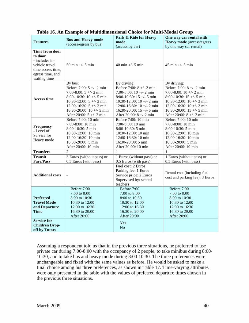
Table 16. An Example of Multidimensional Choice for Multi-Modal Group
Features
Bus and Heavy mode
(access/egress by bus)
Park & Ride for Heavy
mode
(access by car)
One way car rental with
Heavy mode (access/egress by one way car rental)
Time from door
to door
- includes in-vehicle travel time access time, egress time, and waiting time
50 min +/- 5 min 40 min +/- 5 min 45 min +/- 5 min
Access time
By bus:
Before 7:00: 5 +/- 2 min 7:00-8:00: 5 +/- 2 min 8:00-10:30: 10 +/- 5 min 10:30-12:00: 5 +/- 2 min 12:00-16:30: 5 +/- 2 min 16:30-20:00: 10 +/- 5 min After 20:00: 5 +/- 2 min
By driving:
Before 7:00: 8 +/- 2 min 7:00-8:00: 10 +/- 2 min 8:00-10:30: 15 +/- 5 min 10:30-12:00: 10 +/- 2 min 12:00-16:30: 10 +/- 2 min 16:30-20:00: 15 +/- 5 min After 20:00: 8 +/-2 min
By driving:
Before 7:00: 8 +/- 2 min 7:00-8:00: 10 +/- 2 min 8:00-10:30: 15 +/- 5 min 10:30-12:00: 10 +/- 2 min 12:00-16:30: 10 +/- 2 min 16:30-20:00: 15 +/- 5 min After 20:00: 8 +/- 2 min
Frequency
- Level of Service for Heavy mode
Before 7:00: 10 min 7:00-8:00: 10 min 8:00-10:30: 5 min 10:30-12:00: 10 min 12:00-16:30: 10 min 16:30-20:00: 5 min
After 20:00: 10 min
Before 7:00: 10 min 7:00-8:00: 10 min 8:00-10:30: 5 min 10:30-12:00: 10 min 12:00-16:30: 10 min 16:30-20:00: 5 min
After 20:00: 10 min
Before 7:00: 10 min 7:00-8:00: 10 min 8:00-10:30: 5 min 10:30-12:00: 10 min 12:00-16:30: 10 min 16:30-20:00: 5 min
After 20:00: 10 min
Transfers 2 1 1
Transit
Fare/Pass
3 Euros (without pass) or 0.5 Euros (with pass)
1 Euros (without pass) or 0.5 Euros (with pass)
1 Euros (without pass) or 0.5 Euros (with pass)
Additional costs -
Fuel cost: 2 Euros Parking fee: 1 Euros
Service price: 2 Euros Supervised by: school teachers
Rental cost (including fuel cost and parking fee): 3 Euros
Preferred
Travel Mode
and Departure
Time
Before 7:00 7:00 to 8:00 8:00 to 10:30
10:30 to 12:00 12:00 to 16:30 16:30 to 20:00 After 20:00
Before 7:00 7:00 to 8:00 8:00 to 10:30
10:30 to 12:00 12:00 to 16:30 16:30 to 20:00 After 20:00
Before 7:00 7:00 to 8:00 8:00 to 10:30
10:30 to 12:00 12:00 to 16:30 16:30 to 20:00 After 20:00
Service for
Children Drop-
off by Tutors
Yes No
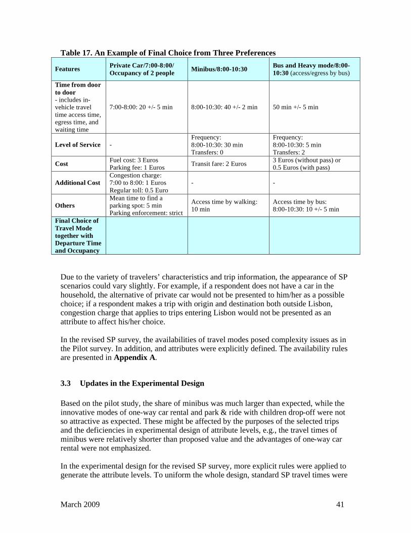
Assuming a respondent told us that in the previous three situations, he preferred to use private car during 7:00-8:00 with the occupancy of 2 people, to take minibus during 8:00-10:30, and to take bus and heavy mode during 8:00-10:30. The three preferences were unchangeable and fixed with the same values as before. He would be asked to make a final choice among his three preferences, as shown in Table 17. Time-varying attributes were only presented in the table with the values of preferred departure times chosen in the previous three situations.
March 2009 41
Table 17. An Example of Final Choice from Three Preferences
Features
Private Car/7:00-8:00/
Occupancy of 2 people Minibus/8:00-10:30
Bus and Heavy mode/8:00-
10:30 (access/egress by bus)
Time from door
to door
- includes in-vehicle travel time access time, egress time, and waiting time
7:00-8:00: 20 +/- 5 min 8:00-10:30: 40 +/- 2 min 50 min +/- 5 min
Level of Service - Frequency:
8:00-10:30: 30 min Transfers: 0
Frequency:
8:00-10:30: 5 min Transfers: 2
Cost Fuel cost: 3 Euros Parking fee: 1 Euros
Transit fare: 2 Euros 3 Euros (without pass) or 0.5 Euros (with pass)
Additional Cost
Congestion charge: 7:00 to 8:00: 1 Euros
Regular toll: 0.5 Euro
- -
Others
Mean time to find a parking spot: 5 min Parking enforcement: strict
Access time by walking: 10 min
Access time by bus: 8:00-10:30: 10 +/- 5 min
Final Choice of
Travel Mode
together with
Departure Time
and Occupancy
Due to the variety of travelers’ characteristics and trip information, the appearance of SP scenarios could vary slightly. For example, if a respondent does not have a car in the household, the alternative of private car would not be presented to him/her as a possible choice; if a respondent makes a trip with origin and destination both outside Lisbon, congestion charge that applies to trips entering Lisbon would not be presented as an attribute to affect his/her choice. In the revised SP survey, the availabilities of travel modes posed complexity issues as in the Pilot survey. In addition, and attributes were explicitly defined. The availability rules are presented in Appendix A.
3.3 Updates in the Experimental Design
Based on the pilot study, the share of minibus was much larger than expected, while the innovative modes of one-way car rental and park & ride with children drop-off were not so attractive as expected. These might be affected by the purposes of the selected trips and the deficiencies in experimental design of attribute levels, e.g., the travel times of minibus were relatively shorter than proposed value and the advantages of one-way car rental were not emphasized. In the experimental design for the revised SP survey, more explicit rules were applied to generate the attribute levels. To uniform the whole design, standard SP travel times were
March 2009 42
calculated based on the travel times, departure times and travel modes of the selected RP trips. The design of attribute values, such as time from door to door, time variability, access time and transfer, was separated when the standard SP travel times <=15 min, 15-30 min, 30-45 min, and > 45 min. Furthermore, there were some rules that captured the inter relationships among travel times and access times of different modes, among costs (e.g. fuel cost and rental cost) and travel times. Fractional factorial design was used and elimination rules were then proposed to refine these initial outcomes, e.g., to delete combinations with a dominate alternative, and to delete combinations with too large differences among travel times and costs of different modes.
March 2009 43
4 Future Plans and Challenges
Generally speaking, the practical design of a SP survey under complex and multiple scenarios is an extremely time-consuming process. Trials and errors are needed to generate artificial but close to reality choice scenarios and attribute values. This large-scale SP survey conducted in Lisbon, Portugal is remarkable and provides a nice example for future applications of SP survey. Up to date, the design for the revised SP survey and experimental exercises has been completed. This survey will be conducted using Internet and computer-assisted personal interviews (CAPI). The programming of SP survey is now at the final stage. The Internet survey will be implemented and data will be collected during March and May in 2009 using mailing lists and divulgation through newspaper and websites in Lisbon, and the CAPI will be conducted during May and June in 2009 to correct the sampling biases. The choice scenarios of the revised SP survey were more complicated and robust than before, which poses challenges to the modeling and estimation in future. There are two problems under discussion: how to model multidimensional choice, and how to deal with a large choice set. Although Multinomial Logit (MNL) models are commonly applied for discrete choice analysis, it is not suitable for the case of multidimensional choice. By virtue of the fact, the alternatives in a multidimensional choice set share observed and also unobserved attributes along various dimensions. There exists a significant amount of literature focusing on the modeling techniques, such as joint logit model and nested logit model for destination and mode choice (Ben-Akiva and Lerman 1985), multinomial probit model for brand choice (Raap and Franses 2000), mixed multinomial logit and ordered logit model for residential location and car ownership decision (Bhat and Guo 2007), error components logit model for time-of-day and mode choice (De Jong et al. 2003), and mixed logit model for vehicle choice (Hess et al. 2006). Different models need to be applied and compared for the revised SP survey data with three-dimensional choice of travel mode, departure time and occupancy. Furthermore, all the alternatives of the large multidimensional choice set were classified based on the 1
st dimension of travel mode into three groups with similarities: car-based
group, public transportation group and multi-modal group. In order to reduce cognitive burden, each respondent was only asked to select the preferred travel mode together with departure time and occupancy in each group per time. Then, three preferred alternatives were assumed unchangeable and presented to the respondent again for a final choice. Though there has been research on approaches to deal with large choice sets in consumer choice settings, e.g., telecom features (Ben-Akiva and Gershenfeld 1998), magazine subscription (McAlister 1979), entertainment services (Venkatesh and Mahajan 1993), and auto-ownership (Hanson and Martin 1990), to our knowledge, there has not been significant research about how to deal with travel choice context where presenting a large number of alternatives is essential given the particular scenarios of application.
March 2009 44
The specific organization of alternatives raised a number of methodological issues. We can explore the following questions in future research.
! Are ‘preference’ and ‘choice’ data inherently different? ! Can they be combined in a consistent manner? ! In the combined data, does the a priori assumption about the nesting structure (the
grouping of alternatives used in the survey) still govern? A possible approach is to compare the estimation results of a particular model with only the ‘choice’ responses and only the ‘preference’ responses against the estimate results of the pooled model (where both ‘preference’ and ‘choice’ responses are considered). A scale parameter needs to be introduced in the pooled model to account for the probable difference in variance. The model performance can be compared later against a model where separate individual specific error terms for ‘preference’ and ‘choice’ responses are tested to capture intra-respondent and inter-respondent heterogeneities (Bliemer et al. 2008, Louviere et al. 2008, Rose et al. 2008).
March 2009 45
References
Alberta, G. and Mahalel, D. (2006). Congestion Tolls and Parking Fees: A Comparison of the Potential Effect on Travel Behavior. Transport Policy, Vol. 13, No. 6, pp. 496-502. Ben-Akiva, M. and Gershenfeld (1998). Multi-featured Products and Services: Analyzing Pricing and Bundling Strategies. Journal of Forecasting, Vol. 17, pp. 175-196. Ben-Akiva, M. and Lerman, S.R. (1985). Discrete Choice Analysis: Theory and Application to Travel Demand. Cambridge, MA: MIT Press. Bhat, C.R. and Castelar, S. (2002). A Unified Mixed Logit Framework for Modeling Revealed and Stated Preferences: Formulation and Application to Congestion Pricing Analysis in the San Francisco Bay Area. Transportation Research Part B, Vol. 36, No. 7, pp. 593-616. Bhat, C.R. and Guo, J.Y. (2007). A Comprehensive Analysis of Built Environment Characteristics on Household Residential Choice and Auto Ownership Levels. Transportation Research Part B, Vol. 41, pp. 506-526. Bliemer, M., Rose, J. and Hensher, D.A. (2008). Constructing Efficient Stated Choice Experiments Allowing for Differences in Error Variances Across Subsets of Alternatives. Transportation Research B, forthcoming. Caussade, S., Ortuzar, J.D., Rizzi, L.I. and Hensher, D.A. (2005). Assessing the Influence of Design Dimensions on Stated Choice Experiment Estimates. Transportation Research Part B, Vol. 39, pp. 621-640. De Jong, G., Daly, A., Pieters, M., Vellay, C., Bradley, M. and Hofman, F. (2003). A Model for Time of Day and Mode Choice Using Error Components Logit. Transportation Research Part E, Vol. 39, pp. 245-268. Hanson, W.A. and Martin, R.K. (1990). Optimal Bundle Pricing. Management Science, Vol. 36, pp. 155-174. Hensher, D.A. (2006). How Do Respondents Process Stated Choice Experiments? Attribute Consideration Under Varying Information Load. Journal of Applied Econometrics, Vol. 21, pp. 861-878. Hensher, D.A. and King, J. (2001). Parking Demand and Responsiveness to Supply, Pricing and Location in the Sydney Central Business District. Transportation Research Part A, Vol. 35, No. 3, pp. 177-196. Hess, S., Train, K.E. and Polak, J.W. (2006). On the Use of a Modified Latin Hypercube Sampling (MLHS) Method in the Estimation of a Mixed Logit Model for Vehicle Choice. Transportation Research Part B, Vol. 40, pp. 147-163.
March 2009 46
Louviere, J.J., Street, D., Burgess, L., Wasi, N., Islam, T. and Marley, A.A.J. (2008). Modeling the Choices of Individual Decision-makers by Combining Efficient Choice Experiment Designs with Extra Preference Information. Journal of Choice Modeling, Vol. 1-1, pp. 128-163. Outwater, M.L., Castleberry, S., Shiftan, Y., Ben-Akiva, M., Zhou, Y.S. and Kuppam, A. (2003). Attitudinal Market Segmentation Approach to Mode Choice and Ridership Forecasting: Structural Equation Modeling. Transportation Research Record, Vol. 1854, pp. 32-42. Raap, R. and Franses, P.H. (2000). A Dynamic Multinomial Probit Model for Brand Choice with Different Long-run and Short-run Effects of Marketing-mix Variables. Journal of Applied Econometrics, Vol. 16, pp. 717-744. Rose, J., Bliemer, M.C., Hensher, D.A. and Collins, A.T. (2008). Designing Efficient Stated Choice Experiments in the Presence of Reference Alternatives. Transportation Research Part B, Vol. 42, pp. 395-406. Sanko, N. (2001). Guidelines for Stated Preference Experiment Design, Master Thesis, Ecole Nationale des Ponts et Chaussees, School of International Management, Research project in association with RAND Europe. Venkatesh, R. and Mahajan, V. (1993). A Probabilistic Approach to Pricing a Bundle of Products or Services. Journal of Marketing Research, November, pp. 494-508. Viegas, J.M., de Abreu e Silva, J. and Arriaga, R. (2008). Innovation in Transport Modes and Services in Urban Areas and their Potential to Fight Congestion. Presented at the 1st Annual Planning Conference on Planning Research, Evaluation in Planning, Porto, Portugal, May 30th.

March 2009 47
Appendix A
Availability of Transport Modes Private car
! Only available for respondents who have a car in the household (driver license not required for passengers), or
! Chose Private car or Car and Heavy mode for their selected RP trip, or ! Mentioned that they have access to a car for the trip even if they chooses public
transportation for selected RP trip One-way car rental
! Only available for respondents who have driver license or whose household members have driver license (as passenger), or
! Chose Private car or Car and Heavy mode for the selected RP trip ! Only available for certain origin-destination pairs with this innovative service ! Not available for trips with purposes such as commute to work, commute to
school, or commute with intermediate stop Regular taxi
! Available for every respondent Shared taxi
! Available for every respondent ! Not available for trips with purposes such as commute to work, commute to
school, or commute with intermediate stop Bus
! Available for every respondent, given that the current bus service in Lisbon has good coverage
Heavy mode ! Only available for certain origin-destination pairs with good coverage of heavy
mode Minibus
! Only available for certain origin-destination pairs with this innovative service ! Only available for trip with purpose such as commute to work, commute to
school, commute with intermediate stop, return home or return home with intermediate stop
! Only available during peak hours 8:00-10:30 and 16:30-20:00 Bus and Heavy mode
! Available for every respondent, given the current bus service in Lisbon has good coverage and the bus routes and heavy mode stations are well connected
Park & Ride for heavy mode ! Use the same rules as private car
One-way car rental with Heavy mode ! Use the same rules as one-way car rental
March 2009 48
Availabilities of Attributes Time-dependent attributes, such as time from door to door, congestion charge, frequency and access/egress time
! For a trip with purpose such as commute to work, commute to school, or commute with intermediate stop, only the alternatives and attribute values for the first four time intervals will be shown to the respondent (before 7:00, 7:00-8:00, 8:00-10:30, and 10:30-12:00). But if the revealed departure time of this trip is after 12:00, all alternatives and attribute values for seven time intervals will be presented to the respondent.
! For a trip with purpose such as return home or return home with intermediate stop, only the alternatives and attribute values for the last four time intervals will be shown to the respondent (10:30-12:00, 12:00-16:30, 16:30-20:00, and after 20:00). But if the revealed departure time of this trip is before 10:30, all alternatives and attribute values for seven time intervals will be presented to the respondent.
Congestion charge ! Only appears for selected RP trip with origin outside Lisbon and destination
inside Lisbon, i.e., trip entering congested area of Lisbon. ! For residents inside Lisbon, there are discounted charges of 80% for their trips
entering Lisbon. Parking fee
! If the last trip of the day is chosen and the trip purpose is return home or return home with intermediate stop, there is no parking fee required (residential parking space).
! If the last trip of the day is chosen and the trip purpose is not return home or return home with intermediate stop (with very small probability), we should discard the last trip of this respondent and choose another RP trip of this respondent, which is better to calculate the parking fee and duration.
Regular toll ! This is the toll for using freeway. This value is fixed and generated based on the
RP trip origin-destination. Transit pass
! The single-trip cost of transit pass is calculated based on its monthly cost, which is around the half cost of transit fare. Its availability is based on the answers regarding to the ownership of transit pass.
! For trip with purpose such as commute to work, commute to school, or commute with intermediate stop, even if the respondent does not have transit pass now, we assume that he will buy and use transit pass in future and the price of transit pass is presented hear instead of the price of single-trip fare.
Service price and supervised by school teachers or professional people ! Only appear here when park & ride for heavy mode is available for the
respondent, the trip purpose is commute with intermediate stop, and the respondent has at least one child in household less than 10 years old who needs to be drop-off.