Page | 1

STAMP User’s Guide v1.08

Statistical Analysis of Metagenomic Profiles

Donovan Parks and Robert Beiko

March 13, 2011

Contents 1. Introduction ........................................................................................................................................................2

2. Contact information ...........................................................................................................................................2

3. Citing STAMP ......................................................................................................................................................2

4. Installation ..........................................................................................................................................................2

4.1 Precompiled binaries for Microsoft Windows ..............................................................................................2

4.2 Source code ..................................................................................................................................................3

4.3 Unit tests: Verifying the installation .............................................................................................................3

5. Analyzing metagenomic profiles ........................................................................................................................3

5.1 Obtaining and constructing metagenomic profiles ......................................................................................3

5.2 Configuring metagenomic profiles for analysis ............................................................................................5

5.3 Exploratory analysis ......................................................................................................................................5

5.4 Statistical techniques in STAMP ...................................................................................................................8

5.5 Filtering results .......................................................................................................................................... 10

5.6 Statistical plots........................................................................................................................................... 11

5.7 Saving plots and tables .............................................................................................................................. 13

5.8 Global preferences .................................................................................................................................... 13

5.9 Empirical tests: Confidence interval coverage and power analysis .......................................................... 14

6. Command-line interface .................................................................................................................................. 14

7. Custom statistical techniques and plots .......................................................................................................... 15

7.1 Creating a custom plot .............................................................................................................................. 16

7.2 Making a plugin publicly available ............................................................................................................. 17

8. References ....................................................................................................................................................... 17

Page | 2

1. Introduction STAMP (STatistical Analysis of Metagenomic Profiles) is a software package for analyzing metagenomic profiles,

such as a phylogenetic profile indicating the number of marker genes assigned to different taxonomic units or a

functional profile indicating the number of sequences assigned to different biological subsystems or pathways. It

aims to promote ‘best practices’ in choosing appropriate statistical techniques and in reporting results by

encouraging the use of effect sizes and confidence intervals for assessing biological importance. A user-friendly,

graphical interface permits easy exploration of statistical results and generation of publication-quality plots for

inferring the biological relevance of features in a metagenomic profile. STAMP is open-source, extensible via a

plugin framework, and available for all major platforms.

This document provides a tutorial style introduction demonstrating how STAMP can be used to analyze

metagenomic profiles. Functional profiles for the obese and lean mouse microbiomes originally investigated by

Turnbaugh et al. (2006) is used to illustrate the use of STAMP.

2. Contact information STAMP is in active development and we are interested in discussing all potential applications of this software.

We encourage you to send us suggestions for new features. Suggestions, comments, and bug reports can be

sent to Rob Beiko (beiko [at] cs.dal.ca). If reporting a bug, please provide as much information as possible and a

simplified version of the data set which causes the bug. This will allow us to quickly resolve the issue.

3. Citing STAMP If you use STAMP in your research, please cite the following article:

Parks, D.H. and Beiko, R.G (2010). Identifying biologically relevant differences between metagenomic

communities. Bioinformatics, 26, 715-721.

4. Installation

4.1 Precompiled binaries for Microsoft Windows

A precompiled binary is available for Microsoft Windows. This binary has been tested under Windows XP and

Windows 7, but should also work under Windows Vista. The precompiled binary is available from the STAMP

website:

http://kiwi.cs.dal.ca/Software/STAMP

If you have a pristine copy of Microsoft Windows installed you may need to install the Visual C++ 2008

Redistributable Package:

Windows XP or x86 (32-bit) versions of Windows Vista or 7

x64 (64-bit) versions of Windows Vista or 7

Page | 3

This package contains a number of commonly required runtime components which you likely already have via

other installed software. STAMP will fail with a message indicating the "configuration is incorrect" if you require

this package.

4.2 Source code

Running from source is the best way to fully exploit and contribute to STAMP. It is relatively painless to setup

STAMP from source on either Microsoft Windows or Apple’s Mac OS X. Instructions on installing STAMP from

source are available on our wiki:

http://kiwi.cs.dal.ca/Software/Quick_installation_instructions_for_STAMP

If you wish to use STAMP strictly from the command-line (e.g., as typical of a cluster environment) only a subset

of the 3rd-party dependencies are required as detailed on the wiki.

4.3 Unit tests: Verifying the installation

A set of unit tests are available to verify that STAMP and all 3rd-party libraries are installed correctly. These unit

tests verify the numerical accuracy of the statistical tests, effect size measures, confidence interval methods,

and multiple test correction methods provided within STAMP. Executing the unit tests is strongly recommended

when installing STAMP from source. To execute the unit tests, move to the main STAMP directory and enter the

following command:

python STAMP_test.py –v

5. Analyzing metagenomic profiles

5.1 Obtaining and constructing metagenomic profiles

Throughout this section we will be looking at the mouse obesity data collected by Turnbaugh et al. (2006). In

this study, the functional potential of the gut microbiota in a lean mouse and an obese mouse were compared

using pyrosequencing. Taxonomic and functional profiles for this data can be obtained from MG-RAST (Meyer et

al., 2008).

Obtaining profiles from MG-RAST: Visit the MG-RAST website (http://metagenomics.nmpdr.org) and browse the

list of pubic metagenomes. Select one of the two mouse projects (LeanMouseCecumMic2005 or

ObeseMouseCecumMic2005). We are interested in obtaining the functional profiles for these projects. To obtain

a functional profile click on the Data Analysis tab above the description of the sample. From the Analysis

Views menu select Functional Classification. From the Data Selection section, click on the + next

to Metagenomes and select the other mouse sample. Set the maximum e-value to 1e-5 and the minimum

alignment length to ~100. Now click the generate button in order to obtain a table with annotated reads from

these two samples. Click on the group table by combobox and select clear grouping in order to obtain

the complete functional table. STAMP requires full MG-RAST tables. To download the functional profile, click on

the download data matching current filter button. Taxonomic profiles can be obtained in a similar

manner.

Page | 4

Creating a STAMP profile: To work with MG-RAST profiles within STAMP they need to be converted into a

STAMP profile. From within STAMP select the Create profile from an MG-RAST table command from

the File menu. This opens up the Create profile dialog box. Leave the profile type as “MG-RAST functional

profile”. Click on the Load profile button and select the mouse functional profile you downloaded. If desired,

you can customize the headings of each hierarchical level by clicking on the Customize headings button.

Click the Create STAMP profile button and save the STAMP profile to a suitable location. We will refer to

this profile as the ObeseMouse profile. If you wish to give the samples more descriptive names, edit the

ObeseMouse.spf file.

IMG/M profiles: Metagenomic profiles can also be obtained from the JGI IMG/M web portal (Markowitz et al.,

2008). Profiles for multiple metagenomic samples can be created using the services at IMG/M and downloaded

as a single file. STAMP works specifically with IMG/M’s abundance profiles obtained by clicking on the Compare

Genomes menu item, followed by Abundance Profile, and finally Abundance Profile Overview.

COG profiles from IMG/M do not contain information about which COG category or higher level class a COG

belongs to. STAMP can add this information to an IMG/M COG profile. This is done in the Assign COG

categories to an IMG/M profile dialog accessible through the File menu. Some COGs are associated

with multiple COG categories. For example, COG0059 is assigned to COG categories E and H. You can elect to

treat multi-code COGs as unique features (i.e., there should be a COG code named EH) or to assign sequences

associated with a multi-code COG to each individual COG category (i.e., a sequence assigned to COG0059 will

add a single count to COG categories E and H).

You can create your own COG profiles and have STAMP assigned higher level COG information to your profile.

The example file Assign_COGs_Example.tsv demonstrates the required file format for using the Assign COG

categories to an IMG/M profile feature of STAMP.

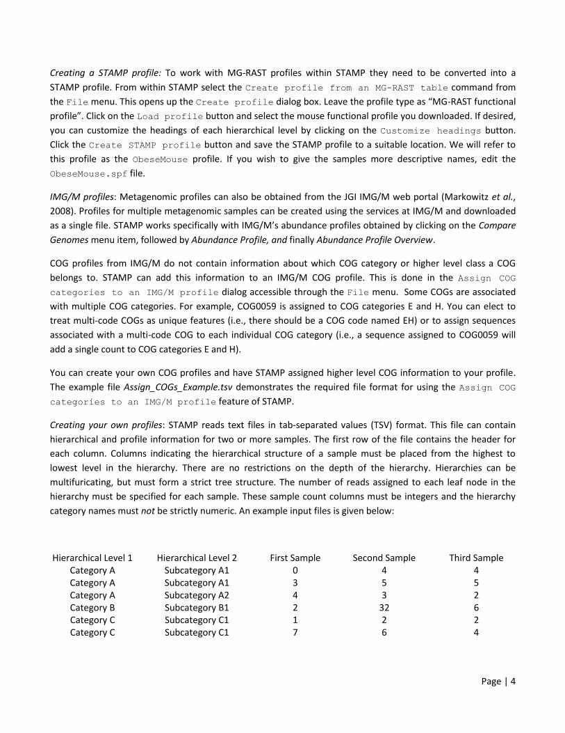
Creating your own profiles: STAMP reads text files in tab-separated values (TSV) format. This file can contain

hierarchical and profile information for two or more samples. The first row of the file contains the header for

each column. Columns indicating the hierarchical structure of a sample must be placed from the highest to

lowest level in the hierarchy. There are no restrictions on the depth of the hierarchy. Hierarchies can be

multifuricating, but must form a strict tree structure. The number of reads assigned to each leaf node in the

hierarchy must be specified for each sample. These sample count columns must be integers and the hierarchy

category names must not be strictly numeric. An example input files is given below:

Hierarchical Level 1 Hierarchical Level 2 First Sample Second Sample Third Sample Category A Subcategory A1 0 4 4 Category A Subcategory A1 3 5 5 Category A Subcategory A2 4 3 2 Category B Subcategory B1 2 32 6 Category C Subcategory C1 1 2 2 Category C Subcategory C1 7 6 4

Page | 5

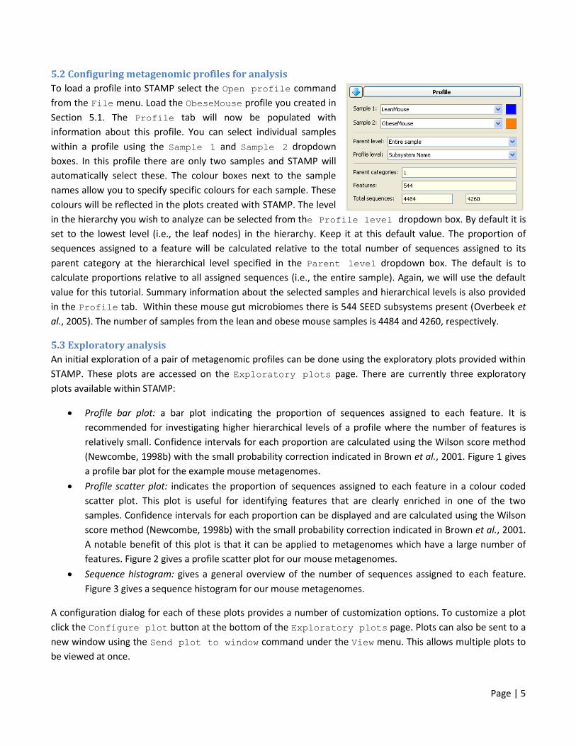
5.2 Configuring metagenomic profiles for analysis

To load a profile into STAMP select the Open profile command

from the File menu. Load the ObeseMouse profile you created in

Section 5.1. The Profile tab will now be populated with

information about this profile. You can select individual samples

within a profile using the Sample 1 and Sample 2 dropdown

boxes. In this profile there are only two samples and STAMP will

automatically select these. The colour boxes next to the sample

names allow you to specify specific colours for each sample. These

colours will be reflected in the plots created with STAMP. The level

in the hierarchy you wish to analyze can be selected from the Profile level dropdown box. By default it is

set to the lowest level (i.e., the leaf nodes) in the hierarchy. Keep it at this default value. The proportion of

sequences assigned to a feature will be calculated relative to the total number of sequences assigned to its

parent category at the hierarchical level specified in the Parent level dropdown box. The default is to

calculate proportions relative to all assigned sequences (i.e., the entire sample). Again, we will use the default

value for this tutorial. Summary information about the selected samples and hierarchical levels is also provided

in the Profile tab. Within these mouse gut microbiomes there is 544 SEED subsystems present (Overbeek et

al., 2005). The number of samples from the lean and obese mouse samples is 4484 and 4260, respectively.

5.3 Exploratory analysis

An initial exploration of a pair of metagenomic profiles can be done using the exploratory plots provided within

STAMP. These plots are accessed on the Exploratory plots page. There are currently three exploratory

plots available within STAMP:

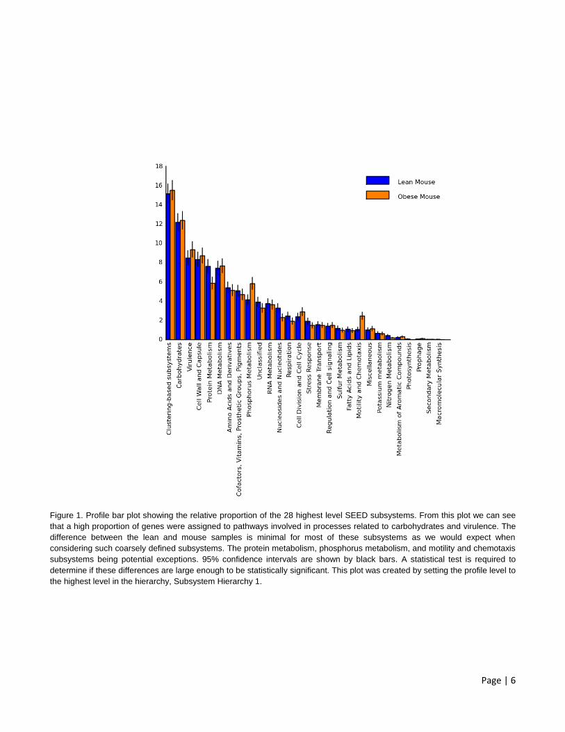
Profile bar plot: a bar plot indicating the proportion of sequences assigned to each feature. It is

recommended for investigating higher hierarchical levels of a profile where the number of features is

relatively small. Confidence intervals for each proportion are calculated using the Wilson score method

(Newcombe, 1998b) with the small probability correction indicated in Brown et al., 2001. Figure 1 gives

a profile bar plot for the example mouse metagenomes.

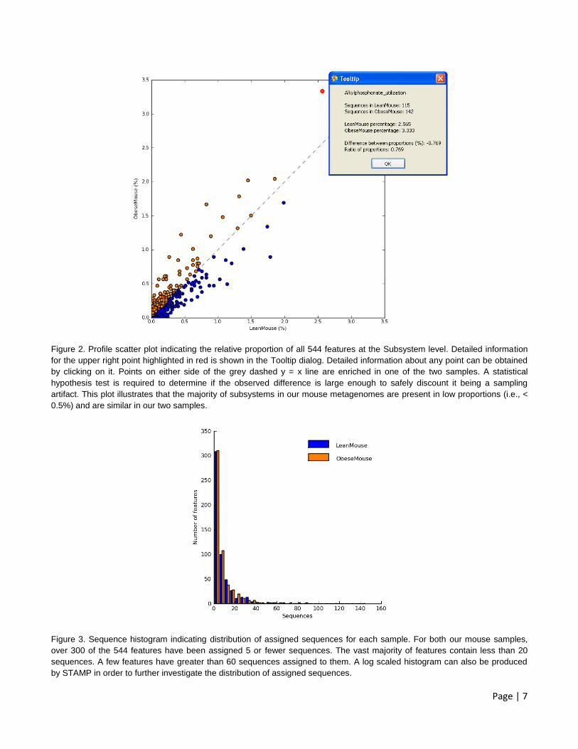
Profile scatter plot: indicates the proportion of sequences assigned to each feature in a colour coded

scatter plot. This plot is useful for identifying features that are clearly enriched in one of the two

samples. Confidence intervals for each proportion can be displayed and are calculated using the Wilson

score method (Newcombe, 1998b) with the small probability correction indicated in Brown et al., 2001.

A notable benefit of this plot is that it can be applied to metagenomes which have a large number of

features. Figure 2 gives a profile scatter plot for our mouse metagenomes.

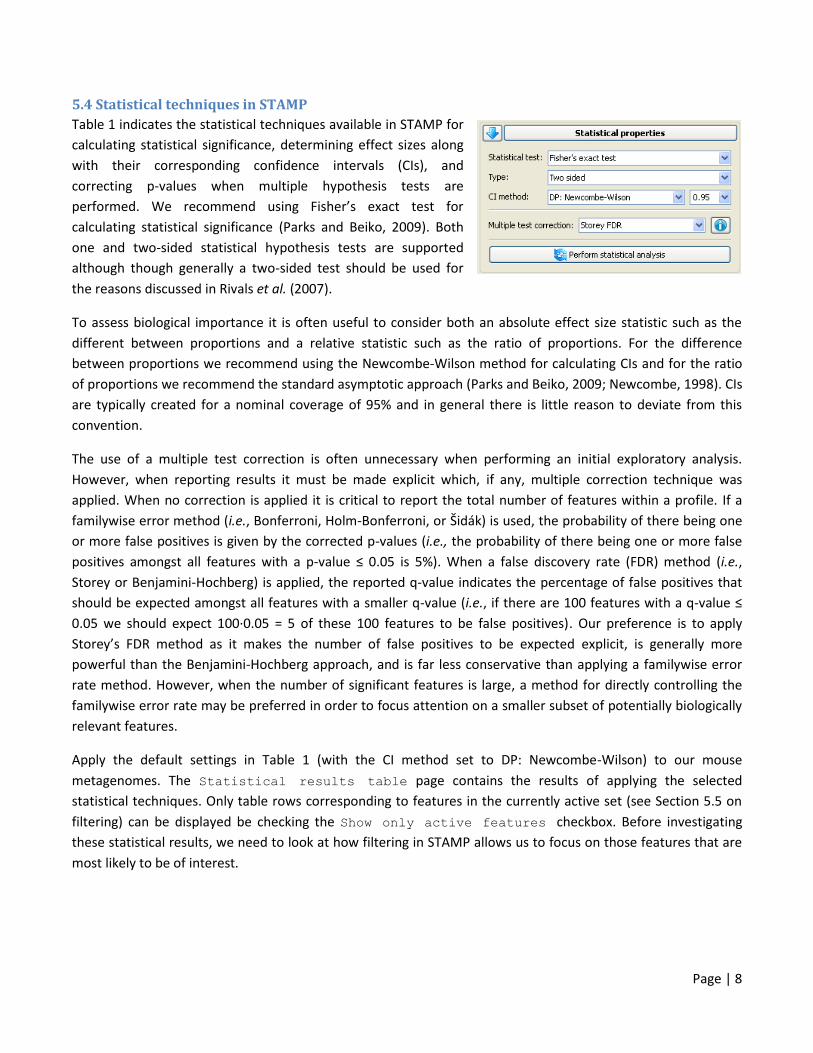
Sequence histogram: gives a general overview of the number of sequences assigned to each feature.

Figure 3 gives a sequence histogram for our mouse metagenomes.

A configuration dialog for each of these plots provides a number of customization options. To customize a plot

click the Configure plot button at the bottom of the Exploratory plots page. Plots can also be sent to a

new window using the Send plot to window command under the View menu. This allows multiple plots to

be viewed at once.

Page | 6

Figure 1. Profile bar plot showing the relative proportion of the 28 highest level SEED subsystems. From this plot we can see

that a high proportion of genes were assigned to pathways involved in processes related to carbohydrates and virulence. The

difference between the lean and mouse samples is minimal for most of these subsystems as we would expect when

considering such coarsely defined subsystems. The protein metabolism, phosphorus metabolism, and motility and chemotaxis

subsystems being potential exceptions. 95% confidence intervals are shown by black bars. A statistical test is required to

determine if these differences are large enough to be statistically significant. This plot was created by setting the profile level to

the highest level in the hierarchy, Subsystem Hierarchy 1.

Page | 7

Figure 2. Profile scatter plot indicating the relative proportion of all 544 features at the Subsystem level. Detailed information

for the upper right point highlighted in red is shown in the Tooltip dialog. Detailed information about any point can be obtained

by clicking on it. Points on either side of the grey dashed y = x line are enriched in one of the two samples. A statistical

hypothesis test is required to determine if the observed difference is large enough to safely discount it being a sampling

artifact. This plot illustrates that the majority of subsystems in our mouse metagenomes are present in low proportions (i.e., <

0.5%) and are similar in our two samples.

Figure 3. Sequence histogram indicating distribution of assigned sequences for each sample. For both our mouse samples,

over 300 of the 544 features have been assigned 5 or fewer sequences. The vast majority of features contain less than 20

sequences. A few features have greater than 60 sequences assigned to them. A log scaled histogram can also be produced

by STAMP in order to further investigate the distribution of assigned sequences.

Page | 8

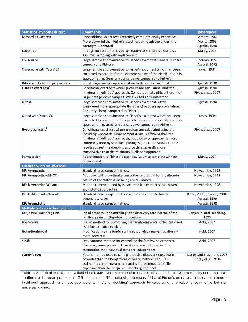
5.4 Statistical techniques in STAMP

Table 1 indicates the statistical techniques available in STAMP for

calculating statistical significance, determining effect sizes along

with their corresponding confidence intervals (CIs), and

correcting p-values when multiple hypothesis tests are

performed. We recommend using Fisher’s exact test for

calculating statistical significance (Parks and Beiko, 2009). Both

one and two-sided statistical hypothesis tests are supported

although though generally a two-sided test should be used for

the reasons discussed in Rivals et al. (2007).

To assess biological importance it is often useful to consider both an absolute effect size statistic such as the

different between proportions and a relative statistic such as the ratio of proportions. For the difference

between proportions we recommend using the Newcombe-Wilson method for calculating CIs and for the ratio

of proportions we recommend the standard asymptotic approach (Parks and Beiko, 2009; Newcombe, 1998). CIs

are typically created for a nominal coverage of 95% and in general there is little reason to deviate from this

convention.

The use of a multiple test correction is often unnecessary when performing an initial exploratory analysis.

However, when reporting results it must be made explicit which, if any, multiple correction technique was

applied. When no correction is applied it is critical to report the total number of features within a profile. If a

familywise error method (i.e., Bonferroni, Holm-Bonferroni, or Šidák) is used, the probability of there being one

or more false positives is given by the corrected p-values (i.e., the probability of there being one or more false

positives amongst all features with a p-value ≤ 0.05 is 5%). When a false discovery rate (FDR) method (i.e.,

Storey or Benjamini-Hochberg) is applied, the reported q-value indicates the percentage of false positives that

should be expected amongst all features with a smaller q-value (i.e., if there are 100 features with a q-value ≤

0.05 we should expect 100·0.05 = 5 of these 100 features to be false positives). Our preference is to apply

Storey’s FDR method as it makes the number of false positives to be expected explicit, is generally more

powerful than the Benjamini-Hochberg approach, and is far less conservative than applying a familywise error

rate method. However, when the number of significant features is large, a method for directly controlling the

familywise error rate may be preferred in order to focus attention on a smaller subset of potentially biologically

relevant features.

Apply the default settings in Table 1 (with the CI method set to DP: Newcombe-Wilson) to our mouse

metagenomes. The Statistical results table page contains the results of applying the selected

statistical techniques. Only table rows corresponding to features in the currently active set (see Section 5.5 on

filtering) can be displayed be checking the Show only active features checkbox. Before investigating

these statistical results, we need to look at how filtering in STAMP allows us to focus on those features that are

most likely to be of interest.

Page | 9

Statistical hypothesis test Comments References Barnard’s exact test Unconditional exact test. Extremely computationally expensive.

More powerful than Fisher’s exact test although the underlying paradigm is debated.

Barnard, 1947 Mehta, 2003 Agresti, 1990

Bootstrap A rough non-parametric approximation to Barnard’s exact test. Assumes sampling with replacement.

Manly, 2007

Chi-square Large sample approximation to Fisher’s exact test. Generally liberal compared to Fisher’s.

Cochran, 1952 Agresti, 1992

Chi-square with Yates’ CC Large sample approximation to Fisher’s exact test which has been corrected to account for the discrete nature of the distribution it is approximating. Generally conservative compared to Fisher’s.

Yates, 1934

Difference between proportions Z-test. Large sample approximation to Barnard’s exact test. Agresti, 1990

Fisher’s exact test1

Conditional exact test where p-values are calculated using the ‘minimum-likelihood’ approach. Computationally efficient even for large metagenomic samples. Widely used and understood.

Agresti, 1990 Rivals et al., 2007

G-test Large sample approximation to Fisher’s exact test. Often considered more appropriate than the Chi-square approximation. Generally liberal compared to Fisher’s.

Agresti, 1990

G-test with Yates’ CC Large sample approximation to Fisher’s exact test which has been corrected to account for the discrete nature of the distribution it is approximating. Generally conservative compared to Fisher’s.

Yates, 1934

Hypergeometric1 Conditional exact test where p-values are calculated using the

‘doubling’ approach. More computationally efficient than the ‘minimum-likelihood’ approach, but the latter approach is more commonly used by statistical packages (i.e., R and StatXact). Our results suggest the doubling approach is generally more conservative than the minimum-likelihood approach.

Rivals et al., 2007

Permutation Approximation to Fisher’s exact test. Assumes sampling without replacement.

Manly, 2007

Confidence interval methods DP: Asymptotic Standard large sample method. Newcombe, 1998

DP: Asymptotic with CC As above, with a continuity correction to account for the discrete nature of the distribution being approximated.

Newcombe, 1998

DP: Newcombe-Wilson Method recommended by Newcombe in a comparison of seven asymptotic approaches.

Newcombe, 1998

OR: Haldane adjustment Standard large sample method with a correction to handle degenerate cases.

Bland, 2000; Lawson, 2004; Agresti, 1999

RP: Asymptotic Standard large sample method. Agresti, 1990

Multiple test correction methods Benjamini-Hochberg FDR Initial proposal for controlling false discovery rate instead of the

familywise error. Step-down procedure. Benjamini and Hochberg,

1995

Bonferroni Classic method for controlling the familywise error. Often criticized as being too conservative.

Adbi, 2007

Holm-Bonferroni Modification to the Bonferroni method which makes it uniformly more powerful.

Adbi, 2007

Šidák Less common method for controlling the familywise error rate. Uniformly more powerful than Bonferroni, but requires the assumption that individual tests are independent.

Adbi, 2007

Storey’s FDR Recent method used to control the false discovery rate. More powerful than the Benjamini-Hochberg method. Requires estimating certain parameters and is more computationally expensive than the Benjamini-Hochberg approach.

Storey and Tibshirani, 2003 Storey et al., 2004

Table 1. Statistical techniques available in STAMP. Our recommendations are indicated in bold. CC = continuity correction, DP

= difference between proportions, OR = odds ratio, RP = ratio of proportions; 1 Use of Fisher’s exact test to imply a ‘minimum-

likelihood’ approach and hypergeometric to imply a ‘doubling’ approach to calculating a p-value is commonly, but not

universally, used.

Page | 10

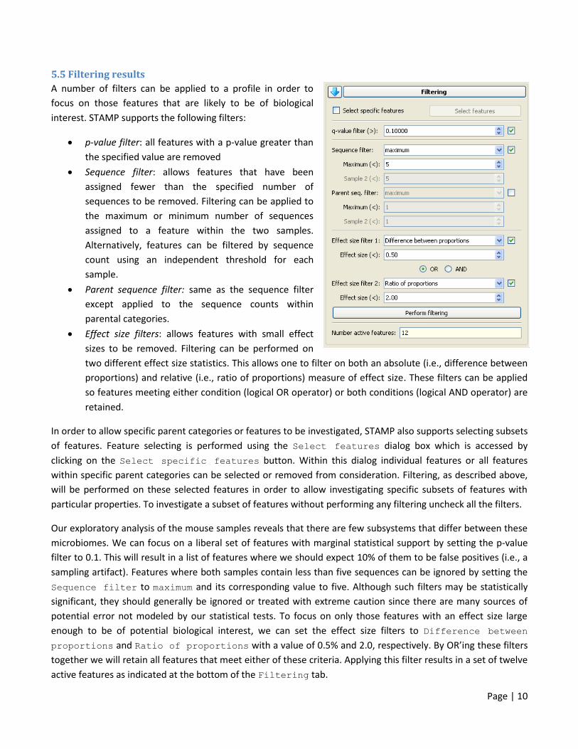
5.5 Filtering results

A number of filters can be applied to a profile in order to

focus on those features that are likely to be of biological

interest. STAMP supports the following filters:

p-value filter: all features with a p-value greater than

the specified value are removed

Sequence filter: allows features that have been

assigned fewer than the specified number of

sequences to be removed. Filtering can be applied to

the maximum or minimum number of sequences

assigned to a feature within the two samples.

Alternatively, features can be filtered by sequence

count using an independent threshold for each

sample.

Parent sequence filter: same as the sequence filter

except applied to the sequence counts within

parental categories.

Effect size filters: allows features with small effect

sizes to be removed. Filtering can be performed on

two different effect size statistics. This allows one to filter on both an absolute (i.e., difference between

proportions) and relative (i.e., ratio of proportions) measure of effect size. These filters can be applied

so features meeting either condition (logical OR operator) or both conditions (logical AND operator) are

retained.

In order to allow specific parent categories or features to be investigated, STAMP also supports selecting subsets

of features. Feature selecting is performed using the Select features dialog box which is accessed by

clicking on the Select specific features button. Within this dialog individual features or all features

within specific parent categories can be selected or removed from consideration. Filtering, as described above,

will be performed on these selected features in order to allow investigating specific subsets of features with

particular properties. To investigate a subset of features without performing any filtering uncheck all the filters.

Our exploratory analysis of the mouse samples reveals that there are few subsystems that differ between these

microbiomes. We can focus on a liberal set of features with marginal statistical support by setting the p-value

filter to 0.1. This will result in a list of features where we should expect 10% of them to be false positives (i.e., a

sampling artifact). Features where both samples contain less than five sequences can be ignored by setting the

Sequence filter to maximum and its corresponding value to five. Although such filters may be statistically

significant, they should generally be ignored or treated with extreme caution since there are many sources of

potential error not modeled by our statistical tests. To focus on only those features with an effect size large

enough to be of potential biological interest, we can set the effect size filters to Difference between

proportions and Ratio of proportions with a value of 0.5% and 2.0, respectively. By OR’ing these filters

together we will retain all features that meet either of these criteria. Applying this filter results in a set of twelve

active features as indicated at the bottom of the Filtering tab.

Page | 11

5.6 Statistical plots

STAMP contains several statistical plots to help investigate the results of the applied statistical techniques and to

identify features that are of biological relevance:

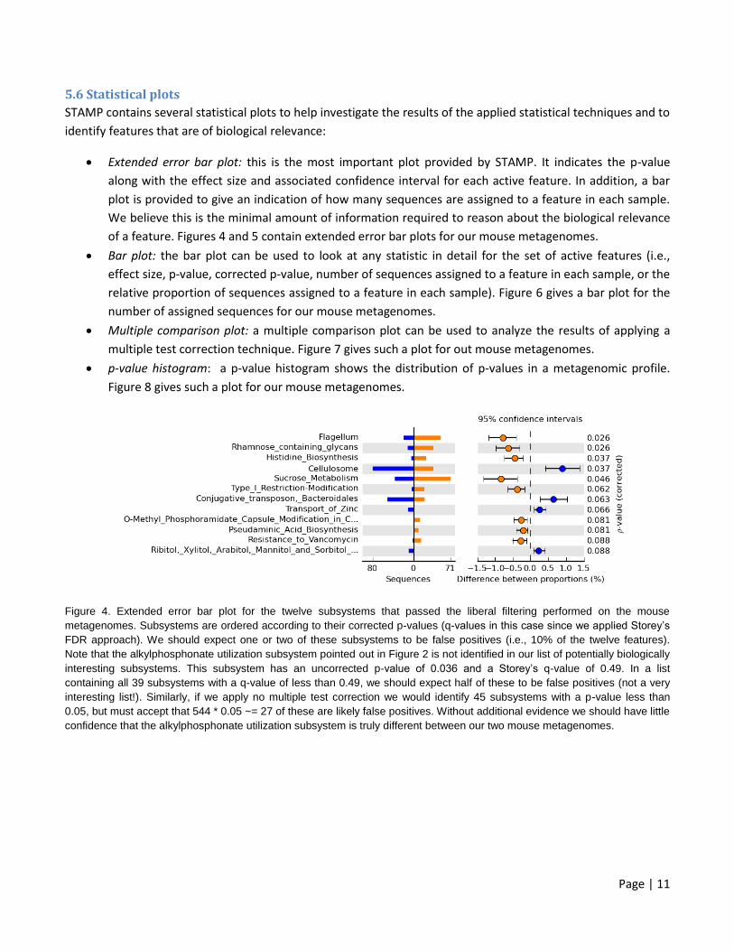
Extended error bar plot: this is the most important plot provided by STAMP. It indicates the p-value

along with the effect size and associated confidence interval for each active feature. In addition, a bar

plot is provided to give an indication of how many sequences are assigned to a feature in each sample.

We believe this is the minimal amount of information required to reason about the biological relevance

of a feature. Figures 4 and 5 contain extended error bar plots for our mouse metagenomes.

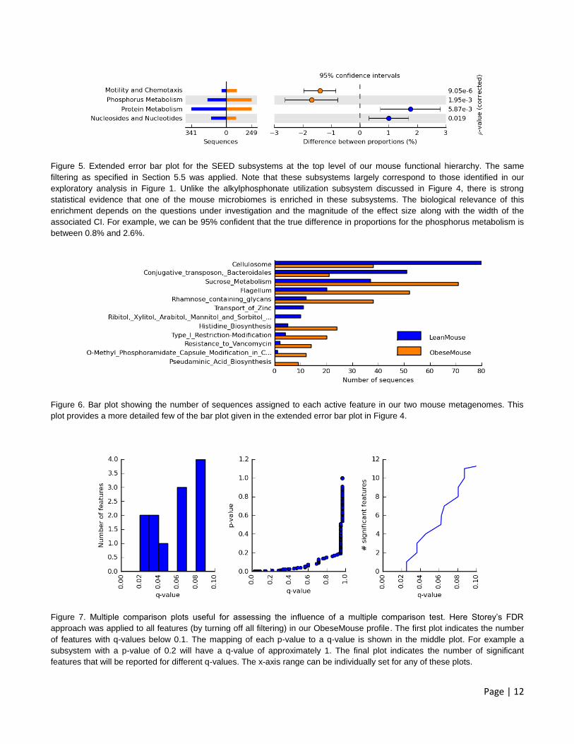
Bar plot: the bar plot can be used to look at any statistic in detail for the set of active features (i.e.,

effect size, p-value, corrected p-value, number of sequences assigned to a feature in each sample, or the

relative proportion of sequences assigned to a feature in each sample). Figure 6 gives a bar plot for the

number of assigned sequences for our mouse metagenomes.

Multiple comparison plot: a multiple comparison plot can be used to analyze the results of applying a

multiple test correction technique. Figure 7 gives such a plot for out mouse metagenomes.

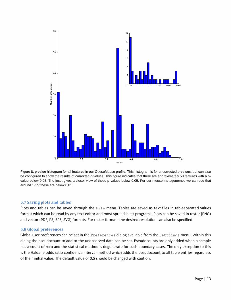
p-value histogram: a p-value histogram shows the distribution of p-values in a metagenomic profile.

Figure 8 gives such a plot for our mouse metagenomes.

Figure 4. Extended error bar plot for the twelve subsystems that passed the liberal filtering performed on the mouse

metagenomes. Subsystems are ordered according to their corrected p-values (q-values in this case since we applied Storey’s

FDR approach). We should expect one or two of these subsystems to be false positives (i.e., 10% of the twelve features).

Note that the alkylphosphonate utilization subsystem pointed out in Figure 2 is not identified in our list of potentially biologically

interesting subsystems. This subsystem has an uncorrected p-value of 0.036 and a Storey’s q-value of 0.49. In a list

containing all 39 subsystems with a q-value of less than 0.49, we should expect half of these to be false positives (not a very

interesting list!). Similarly, if we apply no multiple test correction we would identify 45 subsystems with a p-value less than

0.05, but must accept that 544 * 0.05 ~= 27 of these are likely false positives. Without additional evidence we should have little

confidence that the alkylphosphonate utilization subsystem is truly different between our two mouse metagenomes.

Page | 12

Figure 5. Extended error bar plot for the SEED subsystems at the top level of our mouse functional hierarchy. The same

filtering as specified in Section 5.5 was applied. Note that these subsystems largely correspond to those identified in our

exploratory analysis in Figure 1. Unlike the alkylphosphonate utilization subsystem discussed in Figure 4, there is strong

statistical evidence that one of the mouse microbiomes is enriched in these subsystems. The biological relevance of this

enrichment depends on the questions under investigation and the magnitude of the effect size along with the width of the

associated CI. For example, we can be 95% confident that the true difference in proportions for the phosphorus metabolism is

between 0.8% and 2.6%.

Figure 6. Bar plot showing the number of sequences assigned to each active feature in our two mouse metagenomes. This

plot provides a more detailed few of the bar plot given in the extended error bar plot in Figure 4.

Figure 7. Multiple comparison plots useful for assessing the influence of a multiple comparison test. Here Storey’s FDR

approach was applied to all features (by turning off all filtering) in our ObeseMouse profile. The first plot indicates the number

of features with q-values below 0.1. The mapping of each p-value to a q-value is shown in the middle plot. For example a

subsystem with a p-value of 0.2 will have a q-value of approximately 1. The final plot indicates the number of significant

features that will be reported for different q-values. The x-axis range can be individually set for any of these plots.

Page | 13

Figure 8. p-value histogram for all features in our ObeseMouse profile. This histogram is for uncorrected p-values, but can also

be configured to show the results of corrected q-values. This figure indicates that there are approximately 50 features with a p-

value below 0.05. The inset gives a closer view of those p-values below 0.05. For our mouse metagenomes we can see that

around 17 of these are below 0.01.

5.7 Saving plots and tables

Plots and tables can be saved through the File menu. Tables are saved as text files in tab-separated values

format which can be read by any text editor and most spreadsheet programs. Plots can be saved in raster (PNG)

and vector (PDF, PS, EPS, SVG) formats. For raster formats the desired resolution can also be specified.

5.8 Global preferences

Global user preferences can be set in the Preferences dialog available from the Setttings menu. Within this

dialog the pseudocount to add to the unobserved data can be set. Pseudocounts are only added when a sample

has a count of zero and the statistical method is degenerate for such boundary cases. The only exception to this

is the Haldane odds ratio confidence interval method which adds the pseudocount to all table entries regardless

of their initial value. The default value of 0.5 should be changed with caution.

Page | 14

Feature names within metagenomic profiles are often relatively long. This can make producing plots suitable for

journal publication difficult. The Preferences dialog allows feature names to be truncated to a specific length.

5.9 Empirical tests: Confidence interval coverage and power analysis

STAMP provides two empirical tests which are available from the CI coverage and Power test tabs. Both of

these tests create random bootstrap samples by randomly drawing sequences with replacement from each of

the original samples. That is, the original samples are assumed to perfectly represent the underlying microbial

populations. These tests can either be applied to all features within a profile or to just those passing the user

specified filters.

CI coverage: The CI coverage test allows one to assess the coverage performance of a CI method. An ideal CI

method would produce CI where the proportion of random samples having a CI that contains the true effect size

is equal to the specified nominal level (e.g., 95%). In practice this is difficult to achieve and most methods aim to

be conservative (i.e., they obtain a coverage that is above the specified nominal level). The performance of a CI

method can vary significantly depending on the size of the samples and how many sequences are assigned to a

given feature.

Power test: The power test estimated the type II error rate (i.e., false negative rate) for a statistical hypothesis

test. A type II error occurs when a feature differs between two samples (i.e., the null hypothesis is false), but a

statistical test fails to reject the null hypothesis. The power of a statistical hypothesis test is one minus the type

II error rate. Features that are statistically significant and have low power suggests that there are features with

similar effect sizes in the profile where the statistical test fails to identify them as being statistically significant.

This is a good indication that increased sampling is required.

These tests can take several hours to run when the number of active features is large or when all features are

being considered. We recommend that you perform an initial investigation using a single trial and only a

hundred replicates. If any of the results are of concern a more rigorous test can then be performed.

6. Command-line interface STAMP provide a command-line interface (CLI) to facilitate batch processing or ‘application linking’ as

recommended by Kumar and Dudley (2007). If you are running STAMP from source you can access the CLI by

passing parameters to commandLine.py. The precompiled binary for Microsoft Windows contains a separate CLI

executable (commandLine.exe). Table 2 lists the parameters accepted by the CLI. Command line parameters

taking the name of a statistical method (e.g., --statTest or –effectSizeMeasure1) should be given a parameter

value identical to the name of the method as it appears in the graphical user interface. This allows full support

for the STAMP plugin architecture through the CLI (see Section 7).

As an example, Turnbaugh’s mouse profile can be processed with Fisher’s exact test, 95% confidence intervals

given by the Newcombe-Wilson method, and multiple comparison correction done with Storey’s FDR approach

with the following parameters:

Page | 15

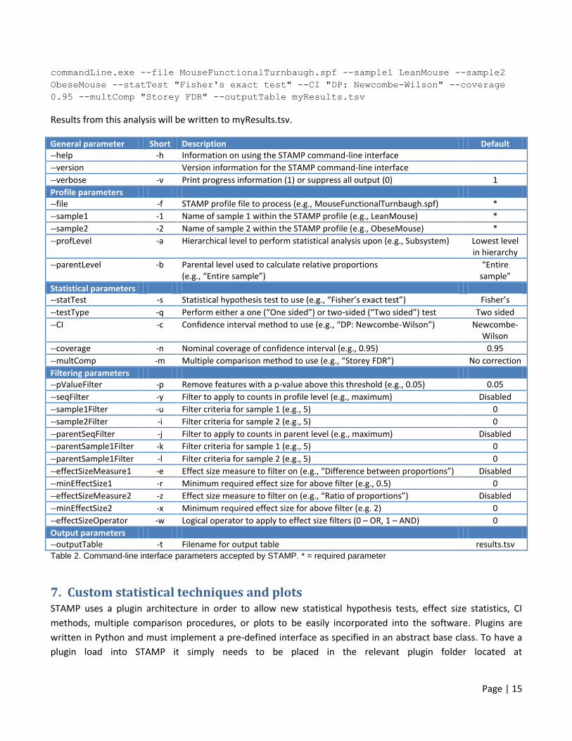
commandLine.exe --file MouseFunctionalTurnbaugh.spf --sample1 LeanMouse --sample2

ObeseMouse --statTest "Fisher's exact test" --CI "DP: Newcombe-Wilson" --coverage

0.95 --multComp "Storey FDR" --outputTable myResults.tsv

Results from this analysis will be written to myResults.tsv.

General parameter Short Description Default --help -h Information on using the STAMP command-line interface

--version Version information for the STAMP command-line interface

--verbose -v Print progress information (1) or suppress all output (0) 1

Profile parameters --file -f STAMP profile file to process (e.g., MouseFunctionalTurnbaugh.spf) *

--sample1 -1 Name of sample 1 within the STAMP profile (e.g., LeanMouse) *

--sample2 -2 Name of sample 2 within the STAMP profile (e.g., ObeseMouse) *

--profLevel -a Hierarchical level to perform statistical analysis upon (e.g., Subsystem) Lowest level in hierarchy

--parentLevel -b Parental level used to calculate relative proportions (e.g., “Entire sample”)

“Entire sample”

Statistical parameters --statTest -s Statistical hypothesis test to use (e.g., “Fisher’s exact test”) Fisher’s

--testType -q Perform either a one (“One sided”) or two-sided (“Two sided”) test Two sided

--CI -c Confidence interval method to use (e.g., “DP: Newcombe-Wilson”) Newcombe-Wilson

--coverage -n Nominal coverage of confidence interval (e.g., 0.95) 0.95

--multComp -m Multiple comparison method to use (e.g., “Storey FDR”) No correction

Filtering parameters --pValueFilter -p Remove features with a p-value above this threshold (e.g., 0.05) 0.05

--seqFilter -y Filter to apply to counts in profile level (e.g., maximum) Disabled

--sample1Filter -u Filter criteria for sample 1 (e.g., 5) 0

--sample2Filter -i Filter criteria for sample 2 (e.g., 5) 0

--parentSeqFilter -j Filter to apply to counts in parent level (e.g., maximum) Disabled

--parentSample1Filter -k Filter criteria for sample 1 (e.g., 5) 0

--parentSample1Filter -l Filter criteria for sample 2 (e.g., 5) 0

--effectSizeMeasure1 -e Effect size measure to filter on (e.g., “Difference between proportions”) Disabled

--minEffectSize1 -r Minimum required effect size for above filter (e.g., 0.5) 0

--effectSizeMeasure2 -z Effect size measure to filter on (e.g., “Ratio of proportions”) Disabled

--minEffectSize2 -x Minimum required effect size for above filter (e.g. 2) 0

--effectSizeOperator -w Logical operator to apply to effect size filters (0 – OR, 1 – AND) 0

Output parameters --outputTable -t Filename for output table results.tsv Table 2. Command-line interface parameters accepted by STAMP. * = required parameter

7. Custom statistical techniques and plots STAMP uses a plugin architecture in order to allow new statistical hypothesis tests, effect size statistics, CI

methods, multiple comparison procedures, or plots to be easily incorporated into the software. Plugins are

written in Python and must implement a pre-defined interface as specified in an abstract base class. To have a

plugin load into STAMP it simply needs to be placed in the relevant plugin folder located at

Page | 16

/STAMP/library/plugins/. All statistical techniques and plots available in STAMP have been implemented as

plugins and can be consulted as examples.

7.1 Creating a custom plot

Here we will create a minimal statistical plot plugin which displays a scatter plot of the relative abundance of all

active features. This will be nearly identical to the exploratory scatter plot that indicates the relative abundance

of all features. To begin, create a file named MyScatterPlot.py in /STAMP/library/plugins/statPlots. It is

important that you place new plugins into the correct plugins folder. To adhere to the required interface for a

statistical plot you must create a new class which is derived from AbstractStatPlotPlugin:

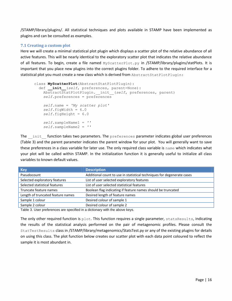
class MyScatterPlot(AbstractStatPlotPlugin):

def __init__(self, preferences, parent=None):

AbstractStatPlotPlugin.__init__(self, preferences, parent)

self.preferences = preferences

self.name = 'My scatter plot'

self.figWidth = 6.0

self.figHeight = 6.0

self.sampleName1 = ''

self.sampleName2 = ''

The __init__ function takes two parameters. The preferences parameter indicates global user preferences

(Table 3) and the parent parameter indicates the parent window for your plot. You will generally want to save

these preferences in a class variable for later use. The only required class variable is name which indicates what

your plot will be called within STAMP. In the initialization function it is generally useful to initialize all class

variables to known default values.

Key Description Pseudocount Additional count to use in statistical techniques for degenerate cases

Selected exploratory features List of user selected exploratory features

Selected statistical features List of user selected statistical features

Truncate feature names Boolean flag indicating if feature names should be truncated

Length of truncated feature names Desired length of feature names

Sample 1 colour Desired colour of sample 1

Sample 2 colour Desired colour of sample 2 Table 3. User preferences are specified in a dictionary with the above keys.

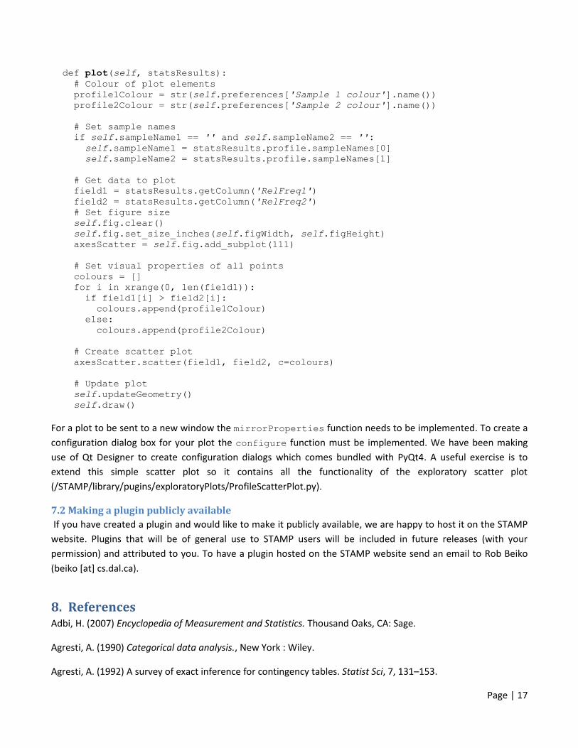
The only other required function is plot. This function requires a single parameter, statsResults, indicating

the results of the statistical analysis performed on the pair of metagenomic profiles. Please consult the

StatTestResults class in /STAMP/library/metagenomics/StatsTest.py or any of the existing plugins for details

on using this class. The plot function below creates our scatter plot with each data point coloured to reflect the

sample it is most abundant in.

Page | 17

def plot(self, statsResults):

# Colour of plot elements

profile1Colour = str(self.preferences['Sample 1 colour'].name())

profile2Colour = str(self.preferences['Sample 2 colour'].name())

# Set sample names

if self.sampleName1 == '' and self.sampleName2 == '':

self.sampleName1 = statsResults.profile.sampleNames[0]

self.sampleName2 = statsResults.profile.sampleNames[1]

# Get data to plot

field1 = statsResults.getColumn('RelFreq1')

field2 = statsResults.getColumn('RelFreq2')

# Set figure size

self.fig.clear()

self.fig.set_size_inches(self.figWidth, self.figHeight)

axesScatter = self.fig.add_subplot(111)

# Set visual properties of all points

colours = []

for i in xrange(0, len(field1)):

if field1[i] > field2[i]:

colours.append(profile1Colour)

else:

colours.append(profile2Colour)

# Create scatter plot

axesScatter.scatter(field1, field2, c=colours)

# Update plot

self.updateGeometry()

self.draw()

For a plot to be sent to a new window the mirrorProperties function needs to be implemented. To create a

configuration dialog box for your plot the configure function must be implemented. We have been making

use of Qt Designer to create configuration dialogs which comes bundled with PyQt4. A useful exercise is to

extend this simple scatter plot so it contains all the functionality of the exploratory scatter plot

(/STAMP/library/pugins/exploratoryPlots/ProfileScatterPlot.py).

7.2 Making a plugin publicly available

If you have created a plugin and would like to make it publicly available, we are happy to host it on the STAMP

website. Plugins that will be of general use to STAMP users will be included in future releases (with your

permission) and attributed to you. To have a plugin hosted on the STAMP website send an email to Rob Beiko

(beiko [at] cs.dal.ca).

8. References Adbi, H. (2007) Encyclopedia of Measurement and Statistics. Thousand Oaks, CA: Sage.

Agresti, A. (1990) Categorical data analysis., New York : Wiley.

Agresti, A. (1992) A survey of exact inference for contingency tables. Statist Sci, 7, 131–153.

Page | 18

Agresti, A. (1999) On logit confidence intervals for the odds ratio with small samples. Biometrics, 55, 597–602.

Barnard, G. A. (1947) Signifiance tests for 2 x 2 tables. Biometrika, 34, 123–138.

Benjamini, Y. and Hochberg, Y. (1995) Controlling the false discovery rate: a practical and powerful approach to

multiple testing. J Roy Stat Soc B, 57, 289–300.

Bland, J. M. and Altman, D. G. (2000) The odds ratio. BMJ, 320, 1468.

Brown, D. B. et al. (2001) Interval estimation for a binomial proportion. Statist Sci, 16, 101-133.

Cochran, W. (1952) The chi-square test of goodness of fit. Ann Math Stat, 23, 315–45.

Kumar, S. and Dudley, J. (2007) Bioinformatics software for biologists in the genomics era. Bioinformatics,

23, 1713–1717.

Lawson, R. (2004) Small sample confidence intervals for odds ratio. Commun Stat Simulat, 33, 1095–1113.

Manly, B. F. J. (2007) Randomization, bootstrap and Monte Carlo methods in biology, Physica Verlag, An Imprint

of Springer-Verlag GmbH.

Markowitz, V. M. et al. (2008) IMG/M: a data management and analysis system for metagenomes. Nucleic Acids

Res, 36 (Database issue), D534–D538.

Mehta, C. R. and Senchaudhuri, P. (2003) Conditional versus unconditional exact tests for comparing two

binomials. http://www.cytel.com/papers/twobinomials.pdf .

Meyer, F. et al. (2008) The metagenomics rast server - a public resource for the automatic phylogenetic and

functional analysis of metagenomes. BMC Bioinformatics, 9, 386.

Newcombe, R. G. (1998) Interval estimation for the difference between independent proportions: comparison of

eleven methods. Stat Med., 17, 873–890.

Newcombe, R.G. (1998b) Two-sided confidence intervals for the single proportion; comparison of several

methods. Stat Med., 17, 857-872.

Overbeek, R. et al. (2005) The subsystems approach to genome annotation and its use in the project to annotate

1000 genomes. Nucleic Acids Res, 33, 5891–5702.

Rivals, I. et al. (2007) Enrichment or depletion of a GO category within a class of genes: which test?

Bioinformatics, 23, 401-407.

Storey, J. D. et al. (2004) Strong control, conservative point estimation, and simultaneous conservative

consistency of false discovery rates: A unified approach. J Roy Stat Soc B, 66, 187–205.

Storey, J. D. and Tibshirani, R. (2003) Statistical significance for genomewide studies. Proc Natl Acad Sci USA,

100, 9440–9445.

Page | 19

Turnbaugh, P. J. et al. (2009) A core gut microbiome in obese and lean twins. Nature, 457, 480–484.

Yates, F. (1934) Contingency table involving small numbers and the χ2 test. Supplement to the Journal of the

Royal Statistical Society, 1, 217-235.