ORIGINAL PAPER - EXPLORATION ENGINEERING

Statistical and numerical density derivatives: example of flowregime diagnosis and permeability k estimation

Victor Torkiowei Biu1 • Shi-Yi Zheng1

Received: 17 April 2016 / Accepted: 31 July 2016 / Published online: 5 April 2017

� The Author(s) 2017. This article is an open access publication

Abstract Presented in this paper are three analytical

approaches. (1) Statistical pressure derivative utilises the

2nd differencing of pressure and time series since pressure

change and subsurface flow rate are nonstationary series

and then integrates the residual of its 1st differences using

simple statistical functions such as sum of square error

SSE, standard deviation, moving average MA and covari-

ance of these series to formulate the model. (2) Pressure–

density equivalent algorithm for each fluid phase is derived

from the fundamental pressure–density relationship and its

derivatives used for diagnosing flow regimes and calcu-

lating permeability. (3) Density transient analytical DTA

solution is derived with the same assumptions as (2) above,

but the density derivatives for each fluid phase are used

along with the semi-log density versus time plot to derive

permeability for each fluid phase. (2) and (3) are solutions

for multiphase flow problems when the fluid density is

treated as a function of pressure with slight change in

density. The first method demonstrated that for field and

design data tested, a good radial stabilisation can be

identified with good permeability estimation without

smoothing the data. Also it showed that in cases investi-

gated, near and far reservoir features can be diagnosed with

clarity. However, the second and third methods can not

only derived each individual phase permeability, the

derivative response from each phase is visualised to give

much clearer picture of the true reservoir response as seen

in the synthetic data analysed which in return ensures that

the derived permeability originates from the formation

radial flow. Summarily, the three methods: statistical

pressure, fluid-phase numerical density and pressure–den-

sity equivalent derivatives gave very clear radial flow sta-

bilisations on the diagnostic plot, from which the reservoir

permeability was derived.

Keywords Numerical density and statistical derivatives �Pressure–density equivalent � Derivatives � Phasepermeabilities � Average permeability k estimation � BHP,PDENO, PDENG, PDENW, PDENA

List of symbols

P Pressure (psi)

T Temperature (�F)R Radius (ft)

K Permeability (md)

Ø Porosity fraction

l Viscosity (cp)

t Time (h)

q Production rate (bbl/day)

B Formation volume factor (rb/Stb)

Ct Total compressibility (psi-1)

rw Wellbore radius (ft)

Dp Change in pressure (psia)

h Formation thickness (ft)

A Drainage area (acres)

Pwf Bottom-hole flowing pressure (psi)

Pi Initial pressure (psi)

tp Cumulative production time

Cs Wellbore storage constant

q Density

c Compressibility

S Skin

& Victor Torkiowei Biu

biut@lsbu.ac.uk

Shi-Yi Zheng

zhengs3@lsbu.ac.uk

1 London South Bank University, 103 Borough Rd, London

SE1 0AA, UK

123

J Petrol Explor Prod Technol (2017) 7:961–976

DOI 10.1007/s13202-017-0341-3

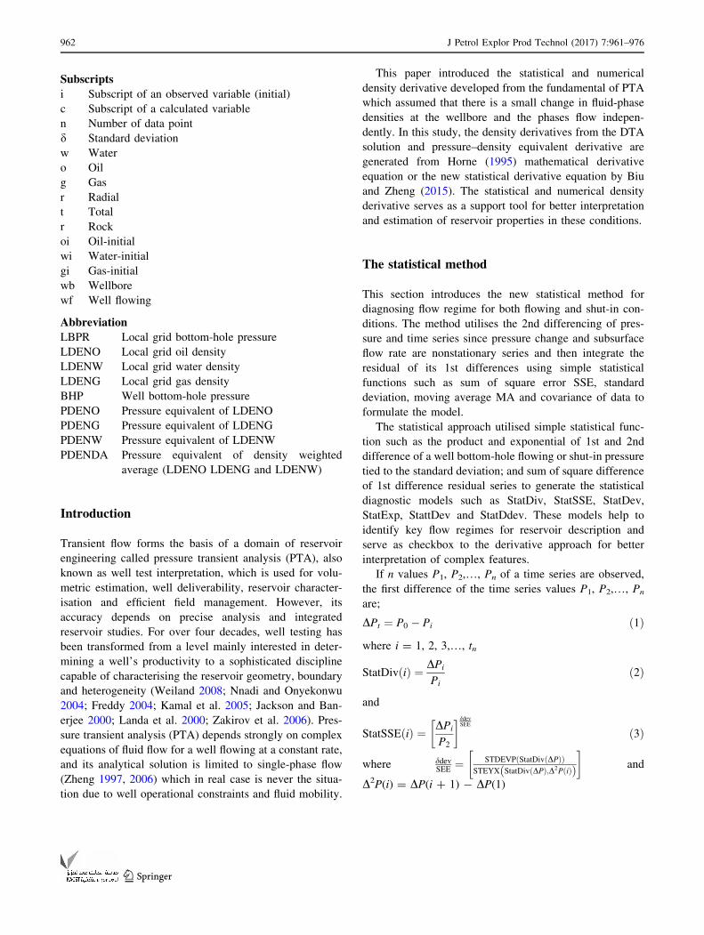
Subscripts

i Subscript of an observed variable (initial)

c Subscript of a calculated variable

n Number of data point

d Standard deviation

w Water

o Oil

g Gas

r Radial

t Total

r Rock

oi Oil-initial

wi Water-initial

gi Gas-initial

wb Wellbore

wf Well flowing

Abbreviation

LBPR Local grid bottom-hole pressure

LDENO Local grid oil density

LDENW Local grid water density

LDENG Local grid gas density

BHP Well bottom-hole pressure

PDENO Pressure equivalent of LDENO

PDENG Pressure equivalent of LDENG

PDENW Pressure equivalent of LDENW

PDENDA Pressure equivalent of density weighted

average (LDENO LDENG and LDENW)

Introduction

Transient flow forms the basis of a domain of reservoir

engineering called pressure transient analysis (PTA), also

known as well test interpretation, which is used for volu-

metric estimation, well deliverability, reservoir character-

isation and efficient field management. However, its

accuracy depends on precise analysis and integrated

reservoir studies. For over four decades, well testing has

been transformed from a level mainly interested in deter-

mining a well’s productivity to a sophisticated discipline

capable of characterising the reservoir geometry, boundary

and heterogeneity (Weiland 2008; Nnadi and Onyekonwu

2004; Freddy 2004; Kamal et al. 2005; Jackson and Ban-

erjee 2000; Landa et al. 2000; Zakirov et al. 2006). Pres-

sure transient analysis (PTA) depends strongly on complex

equations of fluid flow for a well flowing at a constant rate,

and its analytical solution is limited to single-phase flow

(Zheng 1997, 2006) which in real case is never the situa-

tion due to well operational constraints and fluid mobility.

This paper introduced the statistical and numerical

density derivative developed from the fundamental of PTA

which assumed that there is a small change in fluid-phase

densities at the wellbore and the phases flow indepen-

dently. In this study, the density derivatives from the DTA

solution and pressure–density equivalent derivative are

generated from Horne (1995) mathematical derivative

equation or the new statistical derivative equation by Biu

and Zheng (2015). The statistical and numerical density

derivative serves as a support tool for better interpretation

and estimation of reservoir properties in these conditions.

The statistical method

This section introduces the new statistical method for

diagnosing flow regime for both flowing and shut-in con-

ditions. The method utilises the 2nd differencing of pres-

sure and time series since pressure change and subsurface

flow rate are nonstationary series and then integrate the

residual of its 1st differences using simple statistical

functions such as sum of square error SSE, standard

deviation, moving average MA and covariance of data to

formulate the model.

The statistical approach utilised simple statistical func-

tion such as the product and exponential of 1st and 2nd

difference of a well bottom-hole flowing or shut-in pressure

tied to the standard deviation; and sum of square difference

of 1st difference residual series to generate the statistical

diagnostic models such as StatDiv, StatSSE, StatDev,

StatExp, StattDev and StatDdev. These models help to

identify key flow regimes for reservoir description and

serve as checkbox to the derivative approach for better

interpretation of complex features.

If n values P1, P2,…, Pn of a time series are observed,

the first difference of the time series values P1, P2,…, Pn

are;

DPt ¼ P0 � Pi ð1Þ

where i = 1, 2, 3,…, tn

StatDiv ið Þ ¼ DPi

Pi

ð2Þ

and

StatSSE ið Þ ¼ DPi

P2

� �ddevSEE

ð3Þ

where ddevSEE

¼ STDEVP StatDivðDPÞð ÞSTEYX StatDiv DPð Þ;D2P ið Þð Þ

� �and

D2P(i) = DP(i ? 1) - DP(1)

962 J Petrol Explor Prod Technol (2017) 7:961–976

123

Equations (2) and (3) are known as model A and B.

These are similar to semi-log pressure–time curve devel-

oped by Miller et al. (1950) and Horner (1951) but differ

completely in terms of sharp contrast between each flowing

regimes which is clearly seen, thus better approach for

wellbore and reservoir parameters estimation to support

interpretation from conventional, type-curve and derivative

methods. These semi-log models are simple to generate and

good for easy identification of different flow regimes to

obtain reliable reservoir properties.

For better reservoir characterisation, six statistical

models mimicking the log–log pressure derivative

approach are derived using the steps below;

First, the 1st pressure and time differencing are

obtained:

DPt ¼ P0 � Pi

Dtt ¼ tiþ1 � tið4Þ

Then, the divided 1st differencing for pressure and time

is derived:

Ddev ið Þ ¼ DP iþ 1ð ÞDP 2ð Þ ð5Þ

Dttt ¼ Dti=Dtiþ1 ð6Þ

The residual for the pressure and time differencing are

generated using the statistical functions such as standard

deviation between data points:

dDpt ið Þ ¼ STDEV Dtt iþ 1ð Þ; iþ 2ð Þ;D2P iþ 1ð Þ; iþ 2ð Þ� �

ð7Þ

To reduce the noise effect arising from the differencing, the

square root of the standard deviation of the 1st differencing

and the divided 1st differencing for pressure is obtained:

pdd ið Þ ¼ SQRT dDpt ið Þ � STDEV Ddev();D2PðÞ� �� �

Finally, the six statistical models for flow regime

diagnosis are given as:

Model 1:

StatDev1 ið Þ ¼ SQRT pdd ið Þ � Ddev ið Þ � D2P ið Þ� �

ð8Þ

Model 2: The exponential function

StatExp ið Þ ¼ SQRT EXP SQRT D2P� �� �� �

� pdd ið Þ� D2P ið Þ ð9Þ

Model 3:

StatdDev ið Þ ¼ SQRT pdd ið Þ�Ddev ið Þ�D2P ið Þ�D2P ið Þ� �

ð10Þ

Model 4: The time function

StattDev ið Þ ¼ STDEV Dtt ið Þ;Dtt iþ 1ð Þ;ðStatDev ið Þ; StatDev iþ 1ð ÞÞ

StatDev2 ið Þ0:4¼ Dpðiþ 1Þ � DpðiÞð Þ � pddðiÞ � DdevðiÞDpðiÞ

� ExpDttðiÞ

Dttðiþ 1Þ

� �

Model 5:

þffiffiffiffiffiffiffiffiffiffiffiffiffiffiffiffiffiffiffiffiffiffiffiffiffiffiffiffiffiffiffiffiffiffiffiffiffiffiffiffiffiffiffiffiffiffiffit2iþ1 þ t2i� �

� t2i � t2i�1

� �q� dDptðiÞ

DpðiÞ ð11Þ

Model 6:

StatDev3 ið Þ2 ¼ Dpðiþ 1ÞDpð0Þ

� ��

ffiffiffiffiffiffiffiffiffiffiffiDpðiÞ

p

þ ExpDttðiÞ

Dttðiþ 1Þ

� �� dDptðiÞ � pddðiÞ

ð12Þ

Equations (8)–(12) are regarded as statistical pressure

diagnostic models for interpreting pressure transient

data. These are similar to the log–log derivative

method developed by Tiab (1975), Tiab and Kumar

(1976a, b) and Bourdet et al. (1983), and are reliable

diagnostic tools for flow regimes identification and

reservoir characterisation. They are also used for

estimating wellbore and reservoir parameters in order

to support the interpretation from the derivative method

or type-curve after the analysis. The workflows for

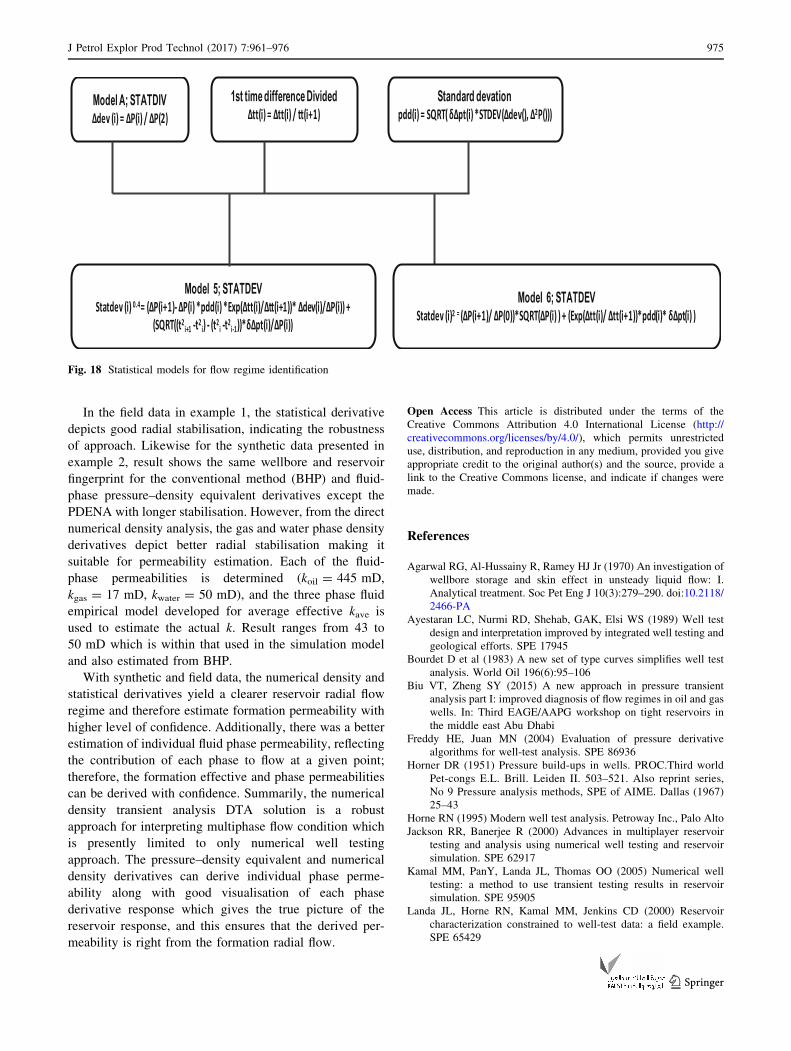
generating these models are shown in Figs. 17 and 18,

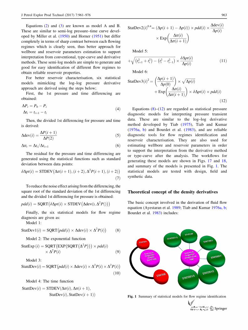
and summary of the models is presented in Fig. 1. The

statistical models are tested with design, field and

synthetic data.

Theoretical concept of the density derivatives

The basic concept involved in the derivation of fluid flow

equation (Ayestaran et al. 1989; Tiab and Kumar 1976a, b;

Bourdet et al. 1983) includes:

Fig. 1 Summary of statistical models for flow regime identification

J Petrol Explor Prod Technol (2017) 7:961–976 963

123

1. Conservation of mass equation,

2. Transport rate equation (e.g. DARCY’s Law),

3. Equation of State

Consider a flow in a cylindrical coordinates with flow in

angular and z-directions neglected, the equations are given

as follows:

Mass rate in�Mass rate outMass rate storage ð13Þ

The above Eq. (1) represents the conservation of mass.

Since the fluid is moving, the equation

q ¼ � k

lAop

orð14Þ

is applied. By conserving mass in an elemental control

volume and applying transport rate equation, the following

equation is obtained:

� 2prhkl

qop

or

� �r

¼ � 2prkhl

qop

or

� �rþDr

þ 2prDrho

otq/ð Þ

ð15Þ

Expanding the equation using Taylor Series

1

r

o

or

rkql

op

or

� �¼ o

otq/½ � ð16Þ

For slight or compressibility liquid,

q ¼ qiec p�pi½ � ð17Þ

Substituting for pressure in the equation, the diffusivity

equation in terms of density is given as:

o2qor2

þ 1

r

oqor

¼ /l cþ cr½ �k

oqot

ð18Þ

o2qor2

þ 1

r

oqor

¼ /lctk

oqot

ð19Þ

Equation (19) is known as the density radial diffusivity

equation which can also be rewritten in form of pressure.

Equations (13)–(19) applies to both liquid and gas. The

density or pressure term in Eq. (19) can be replaced by the

correct expression in terms of density or pressure. Over

four decades, the pressure transient test analysis has

applied the general diffusivity equation in pressure term

to generate several nonunique solutions applying different

well, reservoir and boundaries condition constraints with

pressure-rate data. Equation (19) is rewritten for each

phase as shown below assuming independent fluid-phase

behaviour.

For gas phase

1

r

oqor

roqgor

� �¼

/lgc

kg

oqgot

ð20Þ

For oil phase

1

r

oqor

roqoor

� �¼ /loc

ko

oqoot

ð21Þ

For water phase

1

r

oqor

roqwor

� �¼ /lwc

kw

oqwot

ð22Þ

Invariably as in pressure term for outer and inner

boundary conditions, the density term is also implored as

follows:

o2qor

þ 1

r

oqor

¼ 1

r

o

orroqor

� �¼ 0 ð23Þ

For inner boundary condition

roqor

� �rw

¼ ql2pkh

coiqoi ¼ Constant ð24Þ

Outer boundary condition

q ¼ qe at r ¼ re ð25Þ

Density radial flow equation derivation for each

fluid phase

For slightly and small compressibility fluid such as water

and oil, the isothermal compressibility coefficient c, in

terms of density is given as:

c ¼ 1

qoqop

ð26Þ

Rearranging the parameters w.r.t qP and qq

�c

Z p

pi

dp ¼Z q

qi

oqq

ð27Þ

Integrating

ec Pi�P½ � ¼ qqi

ð28Þ

p ¼ pi �ln q

qi

h ic

ð29Þ

OrApplying the ex expansion series,

ex ¼ 1þ xþ x2

2!þ x3

3!þ � � � þ xn

n!ð30Þ

Because the term c[qi - q] is very small, the ex term

can be approximated as:

ex ¼ 1þ x

Therefore, Eq. (29) can be rewritten as:

q ¼ qi 1� c pi � pð Þ½ �

p ¼ pi �qqiþ 1

c

" #ð31Þ

964 J Petrol Explor Prod Technol (2017) 7:961–976

123

Presently, there are limited oil and gas wells installed

with bottom-hole fluid density gauges for measuring fluid

densities changes at the wellbore during flowing and shut-

in testing conditions. However, for simplification and

application of the density derivative in existing well test

softwares, the density-pressure equivalent equation is

derived.

For slight or compressibility liquid such as oil and

water, the pressure–density equivalent algorithm of the

fluid density changes at the wellbore as derived is given as:

PDENO and PDENW:

p ¼ poi �qqoi

þ 1

co

" #and p ¼ pwi �

qqwi

þ 1

cw

" #ð32Þ

Equations (29) and (31) are the pressure–density

equivalent algorithm for slightly compressible fluid such

as oil and water

From Eqs. (29) and (31),

p ¼ poi �ln q

qoi

h ic

or p ¼ poi �qqoi

þ 1

c

" #

Differentiating with respect to q

oP

oq¼ � 1

coiqoiand oP ¼ � oq

coiqoið33Þ

From Darcy equation flow equation

q ¼ � 2pkhl

roP

orð34Þ

Substitute for qP

q ¼ � 2pkhl

rcoiqoi

oqor

ð35Þ

To derivate the density transient analytical equation for

slightly and small compressibility phase, the following

assumption is applicable:

• There is small change in fluid densities at the wellbore

• The fluid phase flow independently

• Rock density is constant

Radial diffusivity equation for oil phase from Eq. (21) is

given as

1

r

oqor

roqor

� �¼ /lc

k

oqot

ð36Þ

Initial condition

q r; t ¼ 0ð Þ ¼ qi ð37Þ

BC at the wellbore

limr!0

2pkhl

rcoiqoi

oqor

¼ Q ð38Þ

BC at infirmity

limr!1

q r; tð Þ ¼ qi ð39Þ

Applying boundary conditions

Then

q r; tð Þ ¼ qi �lQcoiqoi4pkh

ln2:246kt

/lcr2

� �þ 0:80907

� �ð40Þ

Plotting qwb(t) versus ln (t) will yield a straight line at

longer time and the slope of the line is given as:

oqwbo ln t

¼ moil ¼lQcoiqoi4pkh

ð41Þ

Therefore,

kh ¼ lQcoqo4pmoil

ð42Þ

Similarly for water phase, the radial density equation is

given as:

q r; tð Þ ¼ qi �lQcwiqwi4pkh

ln2:246kt

/lcr2

� �þ 0:80907

� �ð43Þ

Plotting qwb(t) versus ln (t) will yield a straight line at

longer time and the slope of the line is given as:

oqwbo ln t

¼ mwater ¼lQcwiqwi4pkh

ð44Þ

where

kh ¼ lQcwiqwi4pmwater

ð45Þ

Equations (40) and (43) are the density transient

analytical solution for slightly compressible fluid such oil

and water used for generating density derivatives and

specialised density time plot for further interpretation.

For gas phase: for compressible fluid for isothermal

conditions

c ¼ � 1

v

ov

op

� �T

ð46Þ

For real gas equation of state

v ¼ nRTz

p

Differentiating the above equation with respect to

pressure at constant temperature

ov

op

� �T

¼ nRT1

p

oz

op

� �� z

p2

� �ð47Þ

Substituting into Eqs. (47) into (46) gives

cg ¼1

p� 1

z

dz

dp

� �

J Petrol Explor Prod Technol (2017) 7:961–976 965

123

In terms of density

cg ¼1

p� 1

qoqop

� �ð48Þ

This equation is applicable for real gas condition.

Rearranging the parameters w.r.t to qP and qqZ q

qi

oqq

¼Z p

pi

op

p� opcg

� �

Applying the power series for ln p

ln q½ � ¼ q� 1½ � � q� 1½ �2

2þ � � � þ �1½ �n q� 1½ �n

nþ � � � 0\q� 2 ð49Þ

Limit ln x to only the 1st term only

qqi

� �� 1 ¼ p

pi

� �� 1� p� pi½ �cg ð50Þ

For compressible fluid such as gas, the pressure–density

equivalent algorithm as derived is given as: PDENG

p ¼pgiqqo

� p2gicg

1� pgicgð51Þ

Equation (51) is the pressure–density equivalent

algorithm for compressible fluid such as gas. Bottom-hole

flowing or shut-in fluid-phase densities from field, design

or synthetic data generated from simulation software with

wellbore densities keywords for each phase can be

converted to pressure–density equivalent using Eqs. (32)

and (51). Pressure equivalent from the fluid-phase densities

are then analysed in any of the well test software.

Also the density weighted average, PDENA, is used to

obtain the pressure–density equivalent for a two or three

phase combination. The pressure–density equivalent

derived from the densities for all three fluid components

such as gas, oil and water is given as

PDENAPi ¼qgpi þ qopo þ qwpw

qg þ qo þ qwð52Þ

From Eq. (51)

p ¼pgiq� p2giqgicg

qgi 1� pgicg� �

And

op ¼ pgi

qgi 1� pgicg� � oq ð53Þ

From the fundamental real gas equation

n ¼ pv

zRTð54Þ

At standard condition

pv

zT¼ pscvsc

Tsc

q ¼ psc

Tsc

Qsc

5:615zTð Þ ¼ 2pkh

lrpop

orð55Þ

where op ¼ pgi

qgi 1�pgicgð Þ oq and a ¼ pgi

qgi 1�pgicgð Þop ¼ ao q and p ¼ qRzT

From the diffusivity equation for gas

1

r

oqor

roqgor

� �¼

/lgc

kg

oqgot

ð56Þ

Initial condition

q r; t ¼ 0ð Þ ¼ qi ð57Þ

BC at the wellbore

limr!0

4pkhaRl

5:615Tscqsc

� �rq

oqor

¼ Q ð58Þ

BC at infirmity

limr!1

q r; tð Þ ¼ qi ð59Þ

Applying boundary conditionsThen

m qwfð Þ ¼ m qið Þ

� lQ4pkhaR

psc

5:615Tsc

� �ln

2:246kt

/lcr2

� �þ 0:80907

� �

ð60Þom qwbð Þo ln t

¼ mgas ¼lQ

4pkhaRpsc

5:615Tsc

� �ð61Þ

Equation (60) is the density transient analytical solution

for compressible fluid such as gas used for generating

density derivatives and specialised density time plot for

further interpretation.

Plotting qwb2 (t) or m(qwb) versus ln (t) will yield a

straight line at longer time, and the slope of the line is

given as:where

kh ¼ lQ4pkhaR

psc

5:615Tsc

� �1

mgas

ð62Þ

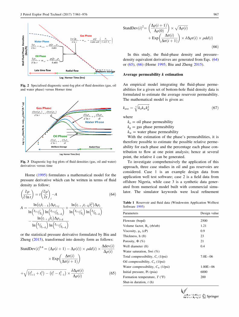
Figure 2 shows example of the specialised semi-log plot

of fluid densities versus time (Horner/Agarwal time,

Horner 1951; Agarwal et al. 1970) for permeability

estimation, and Fig. 3 depicts the expected density

derivatives for each fluid phase generated from Horne

(1995) and Biu and Zheng (2015).

The logarithm density derivative function can be

expressed as;

dDqd ln t

¼ tdDqdt

ð63Þ

966 J Petrol Explor Prod Technol (2017) 7:961–976

123

Horne (1995) formulates a mathematical model for the

pressure derivative which can be written in terms of fluid

density as follow;

oqo ln t

� �¼ t

oqot

� �i

�A ð64Þ

A ¼ln ti=ti � k

� �Dqiþj

ln tiþjti

� �ln tiþj

ti�k

� �þln ti þ jti�k

t2i

� �Dqi

ln tiþjti

� �ln ti=ti�k

� �

�ln ti þ j

ti

� �Dqiþk

ln ti=ti�k

� �ln tiþj

ti�k

� �

or the statistical pressure derivative formulated by Biu and

Zheng (2015), transformed into density form as follows:

StatdDev ið Þ0:4 ¼ Dqðiþ 1Þ � DqðiÞð Þ � qddðiÞ � DdevðiÞDqðiÞ

� ExpDttðiÞ

Dttðiþ 1Þ

� �

þffiffiffiffiffiffiffiffiffiffiffiffiffiffiffiffiffiffiffiffiffiffiffiffiffiffiffiffiffiffiffiffiffiffiffiffiffiffiffiffiffiffiffiffiffiffiffit2iþ1 þ t2i� �

� t2i � t2i�1

� �q� dDqtðiÞ

DqðiÞ ð65Þ

StatdDev ið Þ2¼ Dqðiþ 1ÞDqð0Þ

� ��

ffiffiffiffiffiffiffiffiffiffiffiDqðiÞ

p

þ ExpDttðiÞ

Dttðiþ 1Þ

� �� dDqtðiÞ � qddðiÞ

ð66Þ

In this study, the fluid-phase density and pressure–

density equivalent derivatives are generated from Eqs. (64)

or (65), (66) (Horne 1995; Biu and Zheng 2015).

Average permeability k estimation

An empirical model integrating the fluid-phase perme-

abilities for a given set of bottom-hole fluid density data is

formulated to estimate the average reservoir permeability.

The mathematical model is given as:

kave ¼ffiffiffiffiffiffiffiffiffiffiffiffiffiffikokwk2g

4

qð67Þ

where

ko = oil phase permeability

kg = gas phase permeability

kw = water phase permeability

With the estimation of the phase’s permeabilities, it is

therefore possible to estimate the possible relative perme-

ability for each phase and the percentage each phase con-

tribution to flow at one point analysis; hence at several

point, the relative k can be generated.

To investigate comprehensively the application of this

approach, three case studies in oil and gas reservoirs are

considered. Case 1 is an example design data from

application well test software; case 2 is a field data from

offshore Nigeria, while case 3 is a synthetic data gener-

ated from numerical model built with commercial simu-

lator. The simulator keywords were local refinement

Log Horner Time (hrs)

Wel

l Flu

id P

hase

Den

si�e

s(Ib

m/�

)

()⎟⎟⎠

⎞⎜⎜⎝

⎛==

∂∂

sc

scgas

w

TP

RkhQm

tm

615.54ln απμρ

khQcm

twowo

woterw

πρμρ

4ln==

∂∂

khQcm

too

oilw

πρμρ

4ln==

∂∂

Radial flow Late �me flow Wellbore storage

Gas Phase

Water Phase

Oil Phase

Fig. 2 Specialised diagnostic semi-log plot of fluid densities (gas, oil

and water phase) versus Horner time

Log

Δρ w

f(Ib

m/�

) & Δ

m(ρ

wf)

(Ibm

2 /� 2 .c

p)

Log Horner Time (hrs)

Radial FlowWellbore Storage

( ) ( )dtmdt

tdmd ww ρρ Δ=Δln

dtdt

tdd ww ρρ Δ=Δ

ln

dtdt

tdd oo ρρ Δ=Δ

ln

Fig. 3 Diagnostic log–log plots of fluid densities (gas, oil and water)

derivatives versus time

Table 1 Reservoir and fluid data (Windowstm Application Welltest

Software 1995)

Parameters Design value

Flowrate (bopd) 2500

Volume factor, Bo (rb/stb) 1.21

Viscosity, lo (cP) 0.9

Thickness, h (ft) 23

Porosity, U (%) 21

Well diameter (ft) 0.4

Water saturation, Swi (%)

Total compressibility, Ct (1/psi) 7.0E-06

Oil compressibility, Co (1/psi)

Water compressibility, Cw (1/psi) 1.00E-06

Initial pressure, Pi (psia) 6000

Formation temperature, T (�F) 200

Shut-in duration, t (h)

J Petrol Explor Prod Technol (2017) 7:961–976 967

123

bottom-hole pressure, LBPR; local refinement oil density,

LDENO; local refinement water density, LDENW; local

refinement gas density, LDENG; and well bottom-hole

pressure, BHP, were outputs to obtain the density and

pressure change around the well and as far as the per-

turbation could extend.

Examples

Example 1: design data—low k reservoir with closed

boundary

Table 1 presents a summary of the well and reservoir

data of a designed BHP obtained from the examples of

application well test software (Windowstm Application

Well test Software 1995) simulating the drawdown test

using parameters in Table 1. The reservoir permeability

range is C70 mD, with light oil PVT properties. The

well capacity is above 2500 bbl/days with initial reser-

voir pressure close to 6000 psi. It is required to generate

the pressure–density equivalent and derivative for each

phase, compare their diagnostic signatures and also

estimate the phases permeabilities and average reservoir

permeability

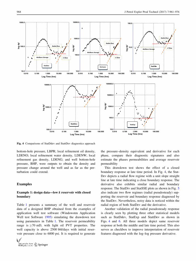
This drawdown test shows the effect of a closed

boundary response at late time period. In Fig. 4, the Stat-

Dev depicts a radial flow regime with a unit slope straight

line at late time indicating a close boundary response. The

derivative also exhibits similar radial and boundary

response. The StatDiv and StatSSE plots as shown in Fig. 5

also indicate two flow regimes (radial pseudosteady) sup-

porting the reservoir and boundary response diagnosed by

the StatDev. Nevertheless, noisy data is noticed within the

radial region of both StatDev and the derivative.

Another validation of the radial pseudosteady response

is clearly seen by plotting three other statistical models

such as StatDdev, StatExp and StattDev as shown in

Figs. 4 and 6. All three models depict same reservoir

response at both the middle and late time period. This also

serves as checkbox to improve interpretation of reservoir

features diagnosed with the log–log pressure derivative.

10.0

100.0

1000.0

0.010 0.100 1.000 10.000 100.000

log

dp'

log

dp'

log

dp'

log

dp'

log

dp'

Log Time (hrs)

Log Time (hrs) Log Time (hrs)

Log Time (hrs) Log Time (hrs)

StatDev

Wellbore Storage

Radial flow

LT flow

10.0

100.0

1000.0

10000.0

0.010 0.100 1.000 10.000 100.000

Derivave

Wellbore Storage

LT flow

Radial flow

1.0

10.0

100.0

0.010 0.100 1.000 10.000 100.000

StatDDev

Wellbore StorageLT flow

Radial flow

100.0

1000.0

10000.0

0.010 0.100 1.000 10.000 100.000

StattDev

10.0

100.0

1000.0

10000.0

100000.0

0.010 0.100 1.000 10.000 100.000

StatExp

Fig. 4 Comparisons of StatDdev and StattDev diagnostics approach

968 J Petrol Explor Prod Technol (2017) 7:961–976

123

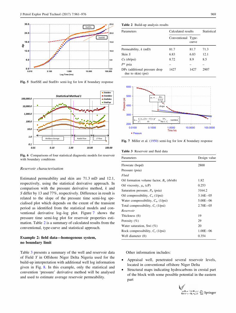
Reservoir characterisation

Estimated permeability and skin are 71.3 mD and 12.1,

respectively, using the statistical derivative approach. In

comparison with the pressure derivative method, k and

S differ by 13 and 77%, respectively. Difference in result is

related to the slope of the pressure time semi-log spe-

cialised plot which depends on the extent of the transient

period as identified from the statistical models and con-

ventional derivative log–log plot. Figure 7 shows the

pressure time semi-log plot for reservoir properties esti-

mation. Table 2 is a summary of calculated results from the

conventional, type-curve and statistical approach.

Example 2: field data—homogenous system,

no boundary limit

Table 3 presents a summary of the well and reservoir data

of Field Y in Offshore Niger Delta Nigeria used for the

build-up interpretation with additional well log information

given in Fig. 8. In this example, only the statistical and

convention ‘pressure’ derivative method will be analysed

and used to estimate average reservoir permeability.

Other information includes:

• Appraisal well, penetrated several reservoir levels,

located in conventional offshore Niger Delta

• Structural maps indicating hydrocarbons in crestal part

of the block with some possible potential in the eastern

part

0.0

5.0

10.0

15.0

20.0

25.0

0.0

6.0

12.0

18.0

24.0

30.0

0.010 0.100 1.000 10.000 100.000

dp

Log Time (hrs)

StatSSE

StatDiv

Fig. 5 StatSSE and StatDiv semi-log for low K boundary response

0.1

1.0

10.0

100.0

1,000.0

10,000.0

100,000.0

0.01 0.10 1.00 10.00 100.00

Sta�s�cal Method 1StatdevStatddevSta�devStatExp

Wellbore Storage Radial Flow LT Flow

Fig. 6 Comparisons of four statistical diagnostic models for reservoir

with boundary conditions

Table 2 Build-up analysis results

Parameters Calculated results Statistical

Conventional Type-

curve

Permeability, k (mD) 81.7 81.7 71.3

Skin S 6.83 6.83 12.1

Cs (rb/psi) 8.72 8.9 8.5

P* psia – – –

DPs (additional pressure drop

due to skin) (psi)

1427 1427 2907

Table 3 Reservoir and fluid data

Parameters Design value

Flowrate (bopd) 2800

Pressure (psia)

Fluid

Oil formation volume factor, Bo (rb/stb) 1.82

Oil viscosity, lo (cP) 0.253

Saturation pressure, Pb (psia) 3164.2

Oil compressibility, Co (1/psi) 3.16E-05

Water compressibility, Cw (1/psi) 5.00E-06

Total compressibility, Ct (1/psi) 2.70E-05

Reservoir

Thickness (ft) 19

Porosity (%) 29

Water saturation, Swi (%) 20

Rock compressibility, Cr (1/psi) 1.00E-06

Well diameter (ft) 0.354

2000

3000

4000

5000

6000

0.0100 0.1000 1.0000 10.0000 100.0000Time hrs

Pres

sure

psi

Pressure

slope

Fig. 7 Miller et al. (1950) semi-log for low K boundary response

J Petrol Explor Prod Technol (2017) 7:961–976 969

123

• Reservoir facies associations and their lateral correla-

tion, high sand to shale ratio, suggesting very good

reservoir potential.

• Amalgamated channel fill or delta front facies associ-

ations constituting continuous coalescing sandstone

bodies in a rather constant stacking pattern.

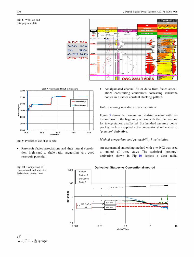
Data screening and derivative calculation

Figure 9 shows the flowing and shut-in pressure with dis-

tortion prior to the beginning of flow with the main section

for interpretation unaffected. Six hundred pressure points

per log circle are applied to the conventional and statistical

‘pressure’ derivative.

Method comparison and permeability k calculation

An exponential smoothing method with a = 0.02 was used

to smooth all three cases. The statistical ‘pressure’

derivative shown in Fig. 10 depicts a clear radial

OWC 2254 TVDSS

G. PAY 26.8mN. PAY 14.7mN/G 54.8%AV. PHI 26.3%AV.SW 35.7 %

Fig. 8 Well log and

petrophysical data

2900

2950

3000

3050

3100

3150

3200

36.5 38.5 40.5 42.5 44.5

Pres

sure

psi

a

Time Hrs

Well A Flowing and Shut-in Pressure

Lower Gauge

Upper Gauge

Fig. 9 Production and shut-in data

0.1

1

10

100

1000

0.001 0.01 0.1 1 10

dp' a

nd d

p

delta T hrs

Derivative: Statdev vs Conventional methodStatdev

Statdev 2

Derivative

Delta P

mhqBk μ2.141=

3178.0 mD

4096.2 mD

Fig. 10 Comparison of

conventional and statistical

derivatives versus time

970 J Petrol Explor Prod Technol (2017) 7:961–976

123

stabilisation fingerprint without boundary effect. The

response behaves like an infinite acting system which is

continuous, without noise. StatDev depicts a continuous

drop in derivative which could be increasing mobility

features away from the well which can be seen from the

well log in Fig. 8; however, there is no available geological

information on increasing thickness away from the well.

The kave estimated from equation k ¼ 141:2qBlmh

is

between 3100 and 4100 mD depending on the movement

of the derivative flat line. This is within the range of

uniform k from core sample and existing well test

interpretation for this reservoir; a good estimation of

permeability is justifiable.

Generally, the field cases reviewed show the robustness

of the statistical ‘pressure’ and numerical density

derivatives applicable in pressure transient analysis. The

results demonstrated that clearer radial flow regimes can

be visualised with increasing confidence on formation

permeability estimation. Also, individual fluid-phase

permeability can be estimated in multiphase condition for

better reservoir characterisation with improved under-

standing of the true contribution of each phase to flow at

the sand face.

Table 4 Reservoir and fluid data

Parameters Design value

Eclipse model Black oil

Model dimension 10 9 5 9 5

Length by width ft by ft 500 9 400

Thickness (ft) 250

Permeability Kx by Ky (mD) 50.0 by 50.0

Porosity (%) 20

Well diameter (ft) 0.60

Initial water saturation Swi (%) 22

Permeability, K (mD) 50

Gas oil contact, GOC (ft) 8820

Oil water contact, OWC (ft) 9000.0

Initial pressure, Pi (psia) 5000.0

Formation temperature, T (�F) 200.0

0.0

0.0

0.1

1.0

10.0

100.0

0.000 0.001 0.010 0.100 1.000 10.000 100.000 1000.000

log

dp'

Log Time (hrs)

Derivatives for Conventional and Pressure-Density Equivalent models

BHP

PENDA

PDENO

PDENG

PDENW

50.8 md

403.7 md

15.8 md

mhqB

kμ2.141

=

Fig. 11 Conventional BHP and three fluid phases pressure–density equivalent derivatives versus time and k estimates. All three fluid phase (gas,

oil and water) with good stabilisation with estimated k for each phase k ¼ 141:2qBlmh

0.001

0.01

0.1

1

10

100

0.0001 0.001 0.01 0.1 1 10 100

log

dp'

Log Time (hrs)

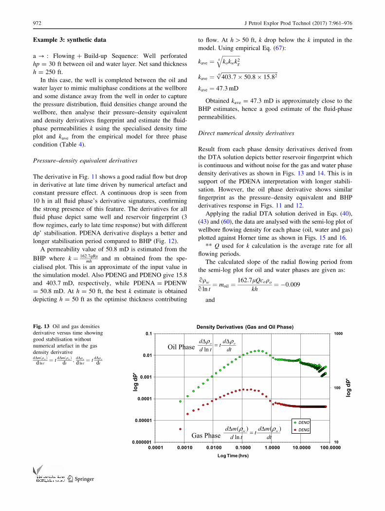
Derivative (Conventional BHP)

BHP

dtt

td ln

d ρΔ = d ρΔ

Fig. 12 Conventional BHP derivative versus time showing good

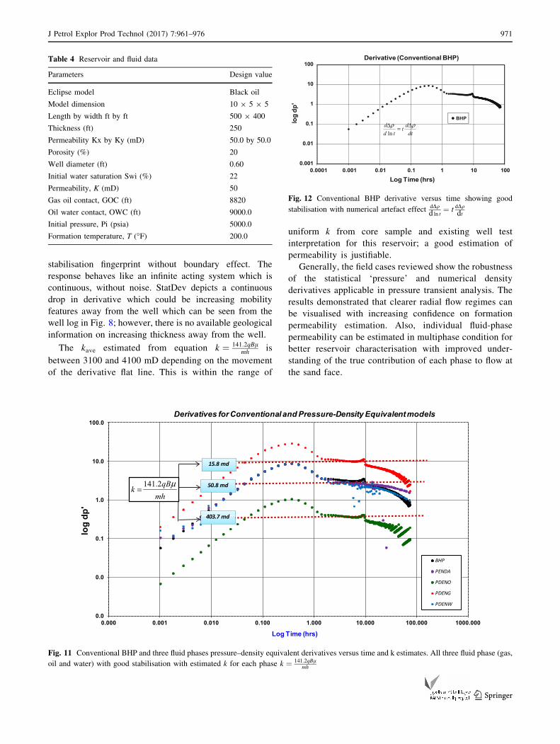
stabilisation with numerical artefact effect dDqd ln t

¼ t dDqdt

J Petrol Explor Prod Technol (2017) 7:961–976 971

123

Example 3: synthetic data

a ? : Flowing ? Build-up Sequence: Well perforated

hp = 30 ft between oil and water layer. Net sand thickness

h = 250 ft.

In this case, the well is completed between the oil and

water layer to mimic multiphase conditions at the wellbore

and some distance away from the well in order to capture

the pressure distribution, fluid densities change around the

wellbore, then analyse their pressure–density equivalent

and density derivatives fingerprint and estimate the fluid-

phase permeabilities k using the specialised density time

plot and kave from the empirical model for three phase

condition (Table 4).

Pressure–density equivalent derivatives

The derivative in Fig. 11 shows a good radial flow but drop

in derivative at late time driven by numerical artefact and

constant pressure effect. A continuous drop is seen from

10 h in all fluid phase’s derivative signatures, confirming

the strong presence of this feature. The derivatives for all

fluid phase depict same well and reservoir fingerprint (3

flow regimes, early to late time response) but with different

dp’ stabilisation. PDENA derivative displays a better and

longer stabilisation period compared to BHP (Fig. 12).

A permeability value of 50.8 mD is estimated from the

BHP where k ¼ 162:7qBlmh

and m obtained from the spe-

cialised plot. This is an approximate of the input value in

the simulation model. Also PDENG and PDENO give 15.8

and 403.7 mD, respectively, while PDENA = PDENW

= 50.8 mD. At h = 50 ft, the best k estimate is obtained

depicting h = 50 ft as the optimise thickness contributing

to flow. At h[ 50 ft, k drop below the k imputed in the

model. Using empirical Eq. (67):

kave ¼ffiffiffiffiffiffiffiffiffiffiffiffiffikokwk2g

4

q

kave ¼ffiffiffiffiffiffiffiffiffiffiffiffiffiffiffiffiffiffiffiffiffiffiffiffiffiffiffiffiffiffiffiffiffiffiffiffiffiffiffiffiffiffi403:7� 50:8� 15:82

4p

kave ¼ 47:3mD

Obtained kave = 47.3 mD is approximately close to the

BHP estimates, hence a good estimate of the fluid-phase

permeabilities.

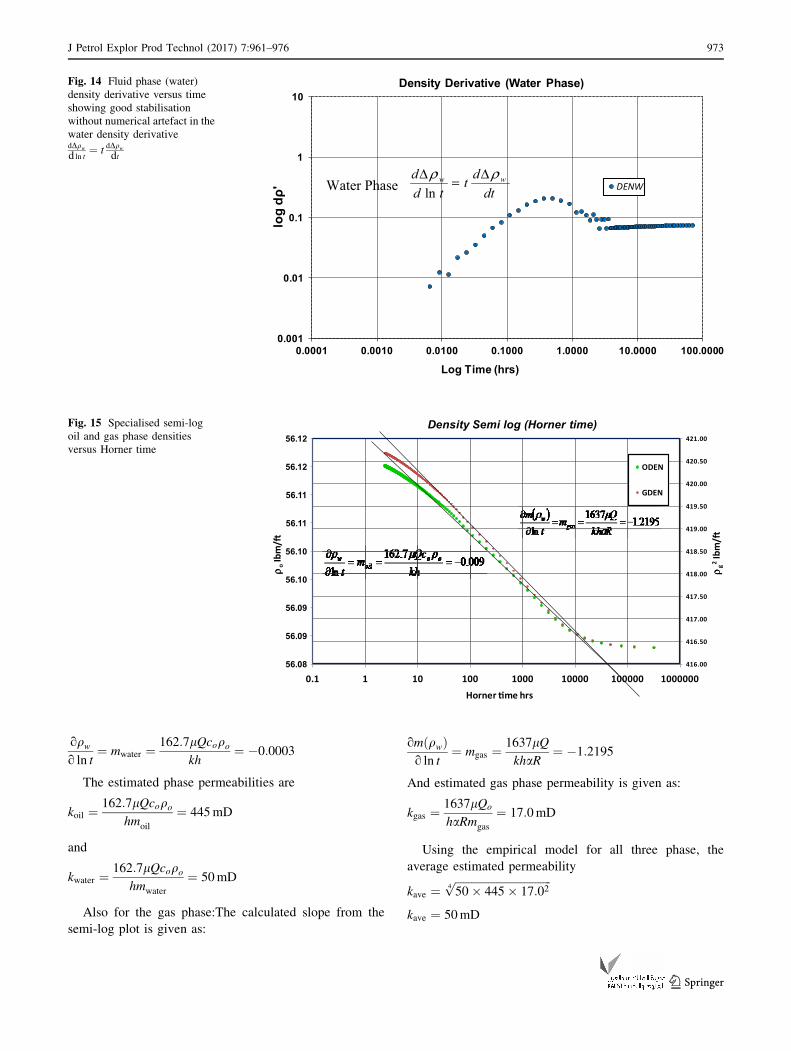
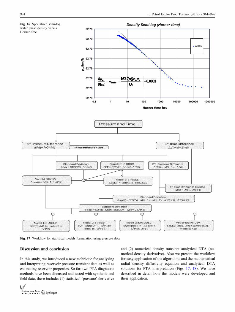
Direct numerical density derivatives

Result from each phase density derivatives derived from

the DTA solution depicts better reservoir fingerprint which

is continuous and without noise for the gas and water phase

density derivatives as shown in Figs. 13 and 14. This is in

support of the PDENA interpretation with longer stabili-

sation. However, the oil phase derivative shows similar

fingerprint as the pressure–density equivalent and BHP

derivatives response in Figs. 11 and 12.

Applying the radial DTA solution derived in Eqs. (40),

(43) and (60), the data are analysed with the semi-log plot of

wellbore flowing density for each phase (oil, water and gas)

plotted against Horner time as shown in Figs. 15 and 16.

** Q used for k calculation is the average rate for all

flowing periods.

The calculated slope of the radial flowing period from

the semi-log plot for oil and water phases are given as:

oqwo ln t

¼ moil ¼162:7lQcoqo

kh¼ �0:009

and

10

100

1000

0.000001

0.00001

0.0001

0.001

0.01

0.1

0.0001 0.0010 0.0100 0.1000 1.0000 10.0000 100.0000

log

d'

log

d'

Log Time (hrs)

Density Derivatives (Gas and Oil Phase)

DENO

DENG( ) ( )dtmdt

tdmd ww ρρ Δ=Δln

Oil Phase

Gas Phase

dtdt

tdd oo ρρ Δ=Δ

ln

Fig. 13 Oil and gas densities

derivative versus time showing

good stabilisation without

numerical artefact in the gas

density derivativedDm qwð Þd ln t

¼ tdDm qwð Þdt

; dDqod ln t

¼ tdDqodt

972 J Petrol Explor Prod Technol (2017) 7:961–976

123

oqwo ln t

¼ mwater ¼162:7lQcoqo

kh¼ �0:0003

The estimated phase permeabilities are

koil ¼162:7lQcoqo

hmoil

¼ 445mD

and

kwater ¼162:7lQcoqo

hmwater

¼ 50mD

Also for the gas phase:The calculated slope from the

semi-log plot is given as:

om qwð Þo ln t

¼ mgas ¼1637lQkhaR

¼ �1:2195

And estimated gas phase permeability is given as:

kgas ¼1637lQo

haRmgas

¼ 17:0mD

Using the empirical model for all three phase, the

average estimated permeability

kave ¼ffiffiffiffiffiffiffiffiffiffiffiffiffiffiffiffiffiffiffiffiffiffiffiffiffiffiffiffiffiffiffiffiffiffiffi50� 445� 17:02

4p

kave ¼ 50mD

0.001

0.01

0.1

1

10

0.0001 0.0010 0.0100 0.1000 1.0000 10.0000 100.0000

log

d'

Log Time (hrs)

Density Derivative (Water Phase)

DENWdtdt

tdd ww ρρ Δ=Δ

lnWater Phase

Fig. 14 Fluid phase (water)

density derivative versus time

showing good stabilisation

without numerical artefact in the

water density derivativedDqwd ln t

¼ tdDqwdt

416.00

416.50

417.00

417.50

418.00

418.50

419.00

419.50

420.00

420.50

421.00

56.08

56.09

56.09

56.10

56.10

56.11

56.11

56.12

56.12

0.1 1 10 100 1000 10000 100000 1000000

ρρ g2

Ibm

/�

ρρ oIb

m/�

Horner �me hrs

Density Semi log (Horner time)

ODEN

GDEN

Fig. 15 Specialised semi-log

oil and gas phase densities

versus Horner time

J Petrol Explor Prod Technol (2017) 7:961–976 973

123

Discussion and conclusion

In this study, we introduced a new technique for analysing

and interpreting reservoir pressure transient data as well as

estimating reservoir properties. So far, two PTA diagnostic

methods have been discussed and tested with synthetic and

field data, these include: (1) statistical ‘pressure’ derivative

and (2) numerical density transient analytical DTA (nu-

merical density derivative). Also we present the workflow

for easy application of the algorithms and the mathematical

radial density diffusivity equation and analytical DTA

solutions for PTA interpretation (Figs. 17, 18). We have

described in detail how the models were developed and

their application.

62.79

62.79

62.79

62.79

62.79

62.79

62.79

62.79

0.1 1 10 100 1000 10000 100000 1000000

ρρ wIb

m/�

Horner �me hrs

Density Semi log (Horner time)

WDEN

Fig. 16 Specialised semi-log

water phase density versus

Horner time

Pressure and Time

1st Time Difference Δt(i)=t(i+1)-t(i)

1st Pressure Difference ΔP(i)= P(0)-P(i) Initial Pressure Fixed

Model 3: STATDDEV SQRT(pdd(i ) x Δdev(i) x

Δ2P(i) x ΔP(i))

Model 4: STATTDEV STDEV( Δtt(i), Δtt(i+1),model1(i),

model1(i+1))

Model 1: STATDEV SQRT(pdd(i ) x Δdev(i) x

Δ2P(i))

Model 2: STATEXP SQRT(Exp(SQRT( Δ2P(i))) x

pdd(i ) x ( Δ2P(i))

1st Time Difference Divided Δtt(i)= Δt(i) / Δt(i+1)

Standard Deviation δΔpt(i) = STDEV( Δtt(i+1), Δtt(i+2), Δ2P(i+1) , Δ2P(i+2))

Model B: STATSSE ΔSSE(i)= Δdev(i) x δdev/SEE

Model A: STATDIV Δdev(i)= ΔP(i+1) / ΔP(2)

Standard E RROR SEE = STEYX ( Δdev(), Δ2P())

Standard Deviation δdev = STDEVP( Δdev())

2nd Pressure Difference Δ2P(i) = ΔP(i+1) - ΔP(i)

Standard Deviation pdd(i) = SQRT( δΔpt(i) x STDEV( Δdev(), Δ2P()))

Fig. 17 Workflow for statistical models formulation using pressure data

974 J Petrol Explor Prod Technol (2017) 7:961–976

123

In the field data in example 1, the statistical derivative

depicts good radial stabilisation, indicating the robustness

of approach. Likewise for the synthetic data presented in

example 2, result shows the same wellbore and reservoir

fingerprint for the conventional method (BHP) and fluid-

phase pressure–density equivalent derivatives except the

PDENA with longer stabilisation. However, from the direct

numerical density analysis, the gas and water phase density

derivatives depict better radial stabilisation making it

suitable for permeability estimation. Each of the fluid-

phase permeabilities is determined (koil = 445 mD,

kgas = 17 mD, kwater = 50 mD), and the three phase fluid

empirical model developed for average effective kave is

used to estimate the actual k. Result ranges from 43 to

50 mD which is within that used in the simulation model

and also estimated from BHP.

With synthetic and field data, the numerical density and

statistical derivatives yield a clearer reservoir radial flow

regime and therefore estimate formation permeability with

higher level of confidence. Additionally, there was a better

estimation of individual fluid phase permeability, reflecting

the contribution of each phase to flow at a given point;

therefore, the formation effective and phase permeabilities

can be derived with confidence. Summarily, the numerical

density transient analysis DTA solution is a robust

approach for interpreting multiphase flow condition which

is presently limited to only numerical well testing

approach. The pressure–density equivalent and numerical

density derivatives can derive individual phase perme-

ability along with good visualisation of each phase

derivative response which gives the true picture of the

reservoir response, and this ensures that the derived per-

meability is right from the formation radial flow.

Open Access This article is distributed under the terms of the

Creative Commons Attribution 4.0 International License (http://

creativecommons.org/licenses/by/4.0/), which permits unrestricted

use, distribution, and reproduction in any medium, provided you give

appropriate credit to the original author(s) and the source, provide a

link to the Creative Commons license, and indicate if changes were

made.

References

Agarwal RG, Al-Hussainy R, Ramey HJ Jr (1970) An investigation of

wellbore storage and skin effect in unsteady liquid flow: I.

Analytical treatment. Soc Pet Eng J 10(3):279–290. doi:10.2118/

2466-PA

Ayestaran LC, Nurmi RD, Shehab, GAK, Elsi WS (1989) Well test

design and interpretation improved by integrated well testing and

geological efforts. SPE 17945

Bourdet D et al (1983) A new set of type curves simplifies well test

analysis. World Oil 196(6):95–106

Biu VT, Zheng SY (2015) A new approach in pressure transient

analysis part I: improved diagnosis of flow regimes in oil and gas

wells. In: Third EAGE/AAPG workshop on tight reservoirs in

the middle east Abu Dhabi

Freddy HE, Juan MN (2004) Evaluation of pressure derivative

algorithms for well-test analysis. SPE 86936

Horner DR (1951) Pressure build-ups in wells. PROC.Third world

Pet-congs E.L. Brill. Leiden II. 503–521. Also reprint series,

No 9 Pressure analysis methods, SPE of AIME. Dallas (1967)

25–43

Horne RN (1995) Modern well test analysis. Petroway Inc., Palo Alto

Jackson RR, Banerjee R (2000) Advances in multiplayer reservoir

testing and analysis using numerical well testing and reservoir

simulation. SPE 62917

Kamal MM, PanY, Landa JL, Thomas OO (2005) Numerical well

testing: a method to use transient testing results in reservoir

simulation. SPE 95905

Landa JL, Horne RN, Kamal MM, Jenkins CD (2000) Reservoir

characterization constrained to well-test data: a field example.

SPE 65429

Model A; STATDIV(i) = ) /

1st time difference Divided(i) = (i) / �(i+1)

Model 5; STATDEVStatdev (i) 0.4 - pdd (i)/

(SQRT((t2i+1 -t2

i) - (t2i -t2

i-1

Standard devationpdd(i) = SQRT( (i) 2P()))

Model 6; STATDEVStatdev (i)2 = ) ) + (Exp( (i)/ (i+1 pdd (i) )

Fig. 18 Statistical models for flow regime identification

J Petrol Explor Prod Technol (2017) 7:961–976 975

123

Miller CC, Dyes AB, Hutchinson CA (1950) Estimation of k and

reservoir pressure from bottom hole pressure buildup character-

istics. Trans AIME 189:91–104

Nnadi M, Onyekonwu M (2004) Numerical well test analysis. SPE

88876

Tiab D (1975) A new approach to detect and locate multiple reservoir

boundaries by transient well pressure data, M.Sc. Thesis. New

Mexico Institute of Mining and Technology, Socorro New

Mexico

Tiab D, Kumar A (1976a) Application of PD function to interference

analysis. In: Paper SPE 6053 presented at the 51st Annual fall

meeting of the society of petroleum engineers of AIME. New

Orleans

Tiab D, Kumar A (1976b) Detection and location of two parallel

sealing fault around a well. In: SPE paper SPE 6056 presented at

the 51st annual fall meeting of the society of petroleum

engineers of AIME. New Orleans

Weiland J, Azari M (2008) Case history review of the application of

pressure transient testing and production logging in monitoring

the performance of the mars deepwater Gulf of Mexico field.

SPE 115591

Windowstm Application Welltest Software (1995). Test and exam-

ples of well test, Demo copy. Petroway Inc., Palo Alto

Zakirov SN, Indrupskiy IM, Zakirov ES, Anikeev DP, Tarasov AI,

Bradulina OV (2006) New approaches in well testing. SPE

100136

Zheng SY (1997) Well testing and characterisation of meandering

fluvial channel reservoirs, Unpublished Ph.D. Thesis. Heriot-

Watt University, p 226

Zheng SY (2006) Fighting against non-unique solution problems in

heterogeneous reservoirs through numerical well testing. In: SPE

Asia Pacific oil and gas conference and exhibition, Adelaide.

SPE 100951

976 J Petrol Explor Prod Technol (2017) 7:961–976

123