Statistical Properties of Kernel PrincipalComponent Analysis

Gilles Blanchard1 & Olivier Bousquet2 & Laurent Zwald3

1 Fraunhofer FIRST (IDA), Kekulestr. 7, D-12489 Berlin, Germany.2 Pertinence, France.

3 Departement de Mathematiques, Universite Paris-Sud, Bat.425, F-91405, France.

Abstract

The main goal of this paper is to prove inequalities on the reconstruction error forKernel Principal Component Analysis. With respect to previous work on this topic,our contribution is twofold: (1) we give bounds that explicitly take into accountthe empirical centering step in this algorithm, and (2) we show that a “localized”approach allows to obtain more accurate bounds. In particular, we show faster ratesof convergence towards the minimum reconstruction error; more precisely, we provethat the convergence rate can typically be faster than n

−1/2. We also obtain a newrelative bound on the error.

A secondary goal, for which we present similar contributions, is to obtain con-vergence bounds for the partial sums of the biggest or smallest eigenvalues of thekernel Gram matrix towards eigenvalues of the corresponding kernel operator. Thesequantities are naturally linked to the KPCA procedure; furthermore these results canhave applications to the study of various other kernel algorithms.

The results are presented in a functional analytic framework, which is suited todeal rigorously with reproducing kernel Hilbert spaces of infinite dimension.

1 Introduction

1.1 Goals of this paper

The main focus of this work is Principal Component Analysis (PCA), and its ’kernelized’variant, Kernel PCA (KPCA). PCA is a linear projection method giving as an outputa sequence of nested linear subspaces which are adapted to the data at hand. This is awidely used preprocessing method with diverse applications, ranging from dimensionalityreduction to denoising. Various extensions of PCA have been explored; applying PCA toa space of functions rather than a space of vectors was first proposed by Besse (1979) (seealso the survey of Ramsay and Dalzell, 1991). Kernel PCA (Scholkopf, Smola, and Muller,1999) is an instance of such a method which has boosted the interest in PCA as it allowsto overcome the limitations of linear PCA in a very elegant manner by mapping the datato a high-dimensional feature space.

For any fixed d, PCA finds a linear subspace of dimension d such that the data linearlyprojected onto it have maximum variance. This is obtained by performing an eigendecom-position of the empirical covariance matrix and considering the span of the eigenvectorscorresponding to the leading eigenvalues. This sets the eigendecomposition of the true

1

covariance matrix as a natural ’idealized’ goal of PCA and begs the question of the re-lationship between this goal and what is obtained empirically. However, despite being arelatively old and commonly used technique, little has been done on analyzing the statisti-cal performance of PCA. Most of the previous work has focused on the asymptotic behaviorof empirical covariance matrices of Gaussian vectors (e.g., Anderson, 1963). Asymptoticresults for PCA have been obtained by Dauxois and Pousse (1976), and Besse (1991) inthe case of PCA in a Hilbert space.

There is, furthermore, an intimate connection between the covariance operator andthe Gram matrix of the data, and in particular between their spectra. In the case ofKPCA, this is a crucial point at two different levels. From a practical point of view, thisconnection allows to reduce the eigendecomposition of the (infinite dimensional) empiricalkernel covariance operator to the eigendecomposition of the kernel Gram matrix, whichmakes the algorithm feasible. From a theoretical point of view, it provides a bridge betweenthe spectral properties of the kernel covariance and those of the so-called kernel integraloperator.

Therefore, theoretical insight on the properties of Kernel PCA reaches beyond thisparticular algorithm alone: it has direct consequences for understanding the spectral prop-erties of the kernel matrix and the kernel operator. This makes a theoretical study ofKernel PCA all the more interesting: the kernel Gram matrix is a central object in allkernel-based methods and its spectrum often plays an important role when studying var-ious kernel algorithms; this has been shown in particular in the case of Support VectorMachines (Williamson, Smola, and Scholkopf, 2001). Understanding the behavior of eigen-values of kernel matrices, their stability and how they relate to the eigenvalues of the corre-sponding kernel integral operator is thus crucial for understanding the statistical propertiesof kernel-based algorithms.

Asymptotical convergence and central limit theorems for estimation of integral oper-ator eigenspectrum by the spectrum of its empirical counterpart have been obtained byKoltchinskii and Gine (2000). Recent work of Shawe-Taylor, Williams, Cristianini, andKandola (2002, 2005) (see also the related work of Braun, 2005) has put forward a finite-sample analysis of the properties of the eigenvalues of kernel matrices and related it to thestatistical performance of Kernel PCA. Our goal in the present work is mainly to extendthe latter results in two different directions:

• In practice, for PCA or KPCA, an (empirical) recentering of the data is generallyperformed. This is because PCA is viewed as a technique to analyze the variance ofthe data; it is often desirable to treat the mean independently as a preliminary step(although, arguably, it is also feasible to perform PCA on uncentered data). Thiscentering was not considered in the cited previous work while we take this step intoaccount explicitly and show that it leads to comparable convergence properties.

• to control the estimation error, Shawe-Taylor et al. (2002, 2005) use what we wouldcall a global approach which typically leads to convergence rates of order n−1/2. Nu-merous recent theoretical works on M-estimation have shown that improved rates canbe obtained by using a so-called local approach, which very coarsely speaking consists

2

in taking the estimation error variance precisely into account. We refer the readerto the works of Massart (2000), Bartlett, Bousquet, and Mendelson (2005), Bartlett,Jordan, and McAuliffe (2003), Koltchinskii (2004) (among others). Applying thisprinciple to the analysis of PCA, we show that it leads to improved bounds.

Note that we consider these two types of extension separately, not simultaneously. Whilewe believe it possible to combine these two results, in the framework of this paper wechoose to treat them independently to avoid additional technicalities. We therefore leavethe local approach in the recentered case as an open problem.

To state and prove our results we use an abstract Hilbert space formalism. Its mainjustification is that some of the most interesting positive definite kernels (e.g., the GaussianRBF kernel) generate an infinite dimensional reproducing kernel Hilbert space (the ”featurespace” into which the data is mapped). This infinite dimensionality potentially raises atechnical difficulty. In part of the literature on kernel methods, a matrix formalism of finite-dimensional linear algebra is used for the feature space, and it is generally assumed moreor less explicitly that the results “carry over” to infinite dimension because (separable)Hilbert spaces have good regularity properties. In the present work, we wanted to staterigorous results directly in an infinite-dimensional space using the corresponding formalismof Hilbert-Schmidt operators and of random variables in Hilbert spaces. This formalismhas been used in other recent work related to ours (Mendelson and Pajor, 2005; Maurer,2004). We hope the necessary notational background which we introduce first will not taxthe reader excessively and hope to convince her that it leads to a more rigorous and elegantanalysis.

One point we want to stress is that, surprisingly maybe, our results are essentiallyindependent of the “kernel” setting. Namely, they hold for any bounded variable takingvalues in a Hilbert space, not necessarily a kernel space. This is why we voluntarilydelay the introduction of kernel spaces until Section 4, after stating our main theorems.We hope that this choice, while possibly having the disadvantage of making the resultsmore abstract at first, will also allow the reader to distinguish more clearly between themathematical framework needed to prove the results and the additional structure broughtforth by considering a kernel space, which allows a richer interpretation of these results,in particular in terms of estimation of eigenvalues of certain integral operators and theirrelationship to the spectrum of the kernel Gram matrix. In a sense, we take here the exactcounterpoint of Shawe-Taylor et al. (2005) who started with studying of the eigenspectrumof the Gram matrix to conclude on the reconstruction error of kernel PCA.

The paper is therefore organized as follows. Section 2 introduces the necessary back-ground on Hilbert spaces, Hilbert-Schmidt operators, and random variables in those spaces.Section 3 presents our main results on the reconstruction error of PCA applied to suchvariables. In Section 4 show how these results are to be interpreted in the framework ofa Reproducing Kernel Hilbert Space and the relation to the eigenspectrum of the kernelGram matrix. In Section 5, we compute numerically the different bounds obtained ontwo ’theoretical’ examples in an effort to paint a general picture of their respective merits.Finally, we conclude in Section 6 with a discussion of various open issues.

3

1.2 Overview of the results

Let us give a quick non-technical overview of the results to come. Let Z be a randomvariable taking values in a Hilbert space H . If we fix the target dimension d of theprojected data, the goal is to recover an optimal d-dimensional space Vd such that theaverage squared distance between a datapoint Z and its projection on Vd is minimum.This quantity is called the (true) reconstruction error and denoted R(Vd). Using available

data, this optimal subspace is estimated by Vd using the PCA procedure, which amountsto minimizing the empirical reconstruction error. One of the quantities we are interestedin is to upper bound the so-called (true) excess error of Vd as compared to the optimal Vd,

that is, R(Vd)−R(Vd) (which is always nonnegative, by definition). Note that the bounds

we obtain are only valid with high probability, since R(Vd) is a random quantity.Our reference point is an inequality, here dubbed “global bound”, obtained by Shawe-

Taylor et al. (2005), taking the form

R(Vd) −R(Vd) .

√d

ntrC ′

2 , (1)

where tr denotes the trace, and C ′2 is a certain operator related to the fourth moments

of the variable. By the symbol . we mean that we are forgetting (for the purposes ofthis section) about some terms considered lower-order, and that the inequality is true upto a finite multiplicative constant. This inequality is recalled in Theorem 3.1, with someminor improvements over the original bound of Shawe-Taylor et al. As a first improvementobtained in Theorem 3.5, we prove that this bound also holds if the data is empiricallyrecentered in the PCA procedure (which is often the case, but was not taken into accountin the above bound).

Next, we prove two different inequalities improving on the bound (1). Both of them relyon a certain quantity ρ(d, n), which depends on the decay of the eigenvalues of operatorC ′

2, and is always smaller than the right-hand side of (1). The first inequality, dubbed“excess bound”, reads (Theorem 3.2)

R(Vd) −R(Vd) . Bdρ(d, n) , (2)

where Bd . (R(Vd) −R(Vd−1))−1 . The second inequality, dubbed “relative bound”, reads

(Theorem 3.4)

R(Vd) −R(Vd) .√R(Vd)ρ(d, n) + ρ(d, n) . (3)

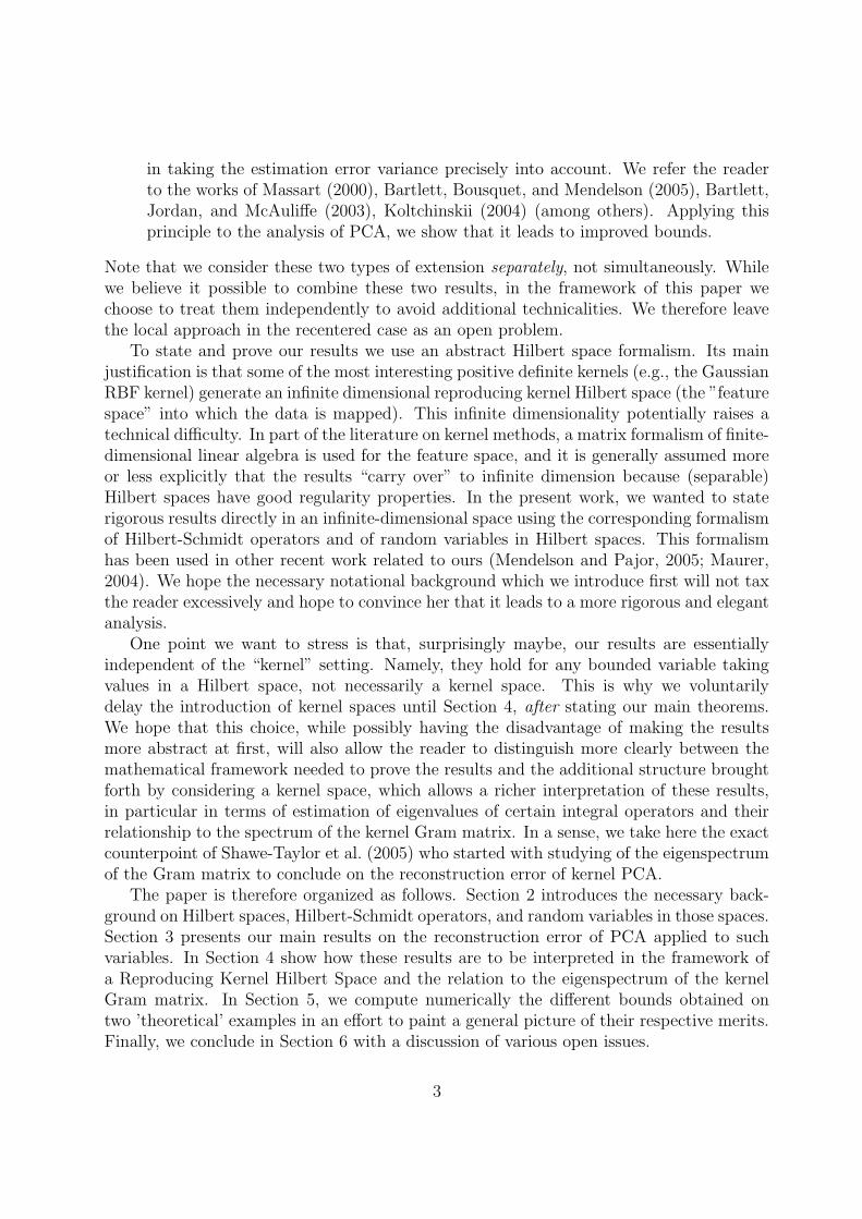
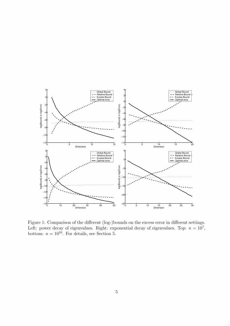
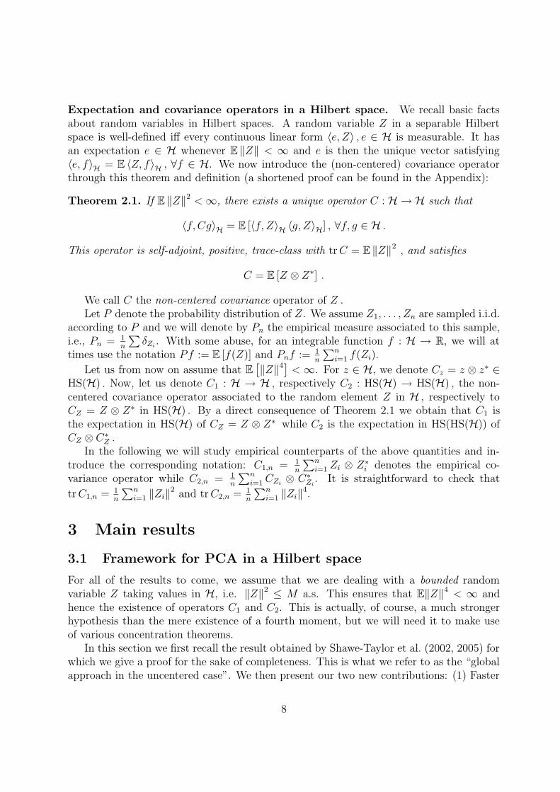
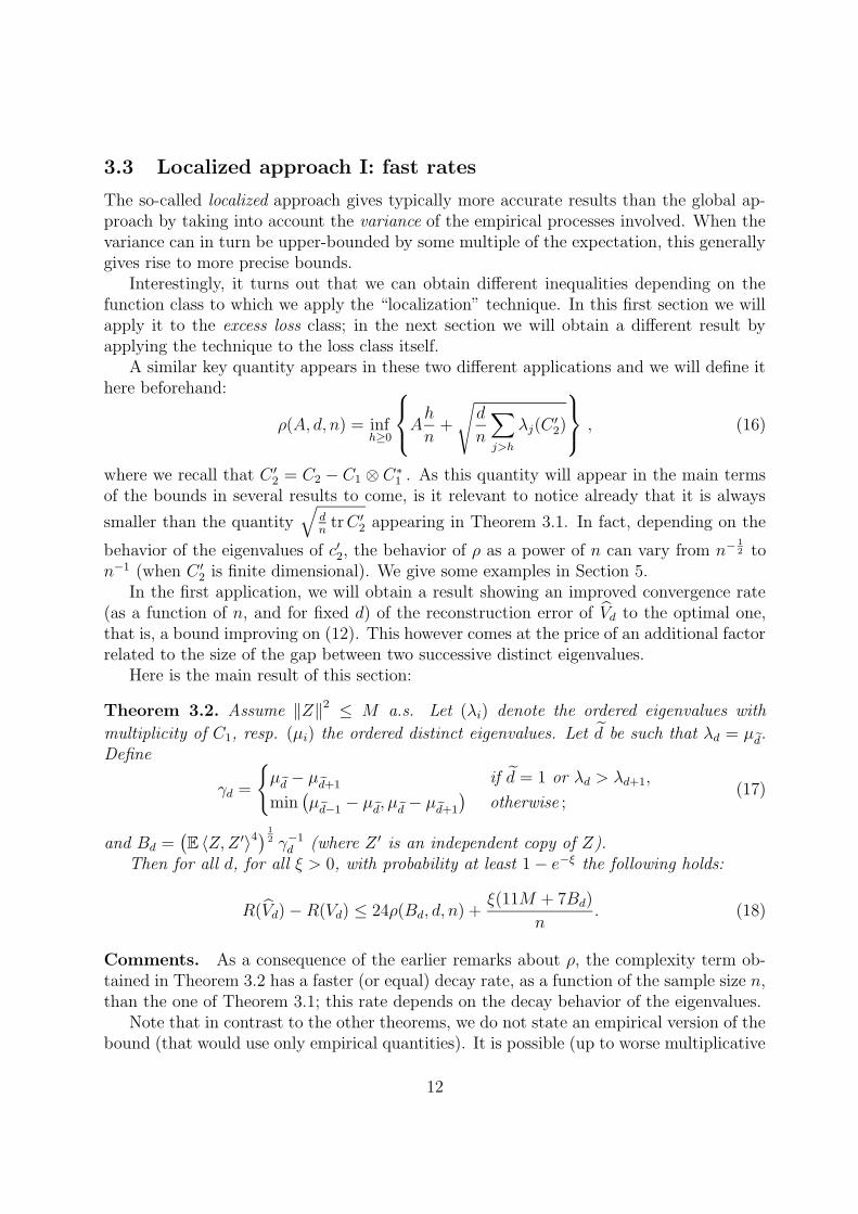
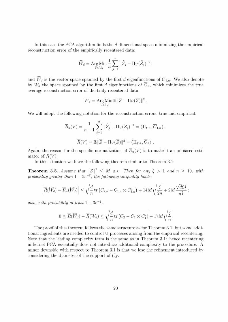
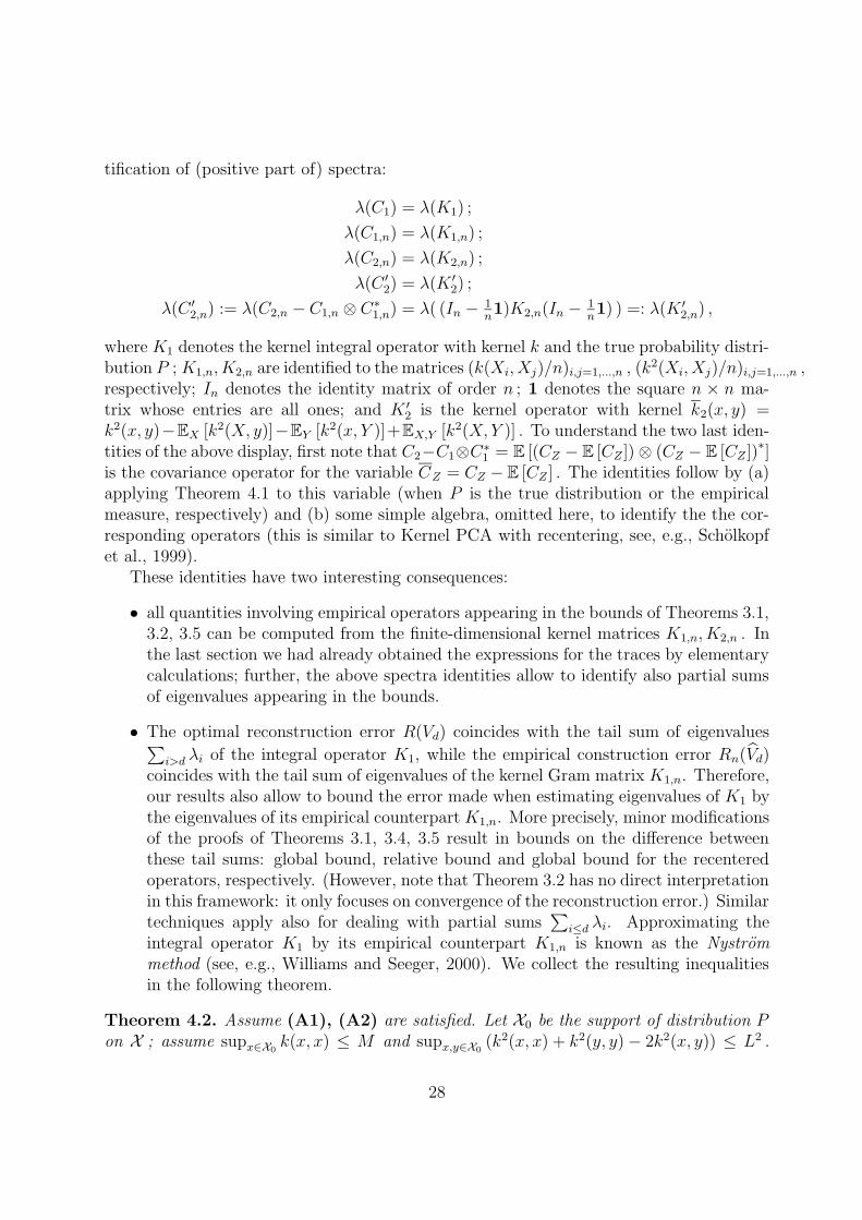
It is valid under the stronger assumption that the variable Z has a constant norm a.s. :this is the case in particular for Kernel PCA when a translation invariant kernel is used.Typically, we expect that (2) exhibits a better behavior than (1) for fixed d when n growslarge, while the converse is true for (3) (it will be better than (1) for fixed n and larged). To illustrate what amounts to a possibly confusing picture, we plotted these differentbounds on two examples (details are given in Section 5). The result appears in Figure 1.The conclusion is that, at least when n is large enough, the best bound between (2) and (3)

4

0 5 10 15−12

−10

−8

−6

−4

−2

0

2

Dimension

log(

Bou

nd) o

r log

(Err

or)

Global BoundRelative BoundExcess BoundOptimal error

0 5 10 15 20−14

−12

−10

−8

−6

−4

−2

0

2

4

Dimension

log(

Bou

nd) o

r log

(Err

or)

Global BoundRelative BoundExcess BoundOptimal error

0 10 20 30 40 50−16

−14

−12

−10

−8

−6

−4

−2

0

2

Dimension

log(

Bou

nd) o

r log

(Err

or)

Global BoundRelative BoundExcess BoundOptimal error

0 5 10 15 20 25 30−25

−20

−15

−10

−5

0

5

Dimension

log(

Bou

nd) o

r log

(Err

or)

Global BoundRelative BoundExcess BoundOptimal error

Figure 1: Comparison of the different (log-)bounds on the excess error in different settings.Left: power decay of eigenvalues. Right: exponential decay of eigenvalues. Top: n = 107,bottom: n = 1010. For details, see Section 5.

5

always beats the original bound (1) (and this, by orders of magnitude). Finally, we showthat all bounds except (2) have also an empirical counterpart, by which we mean that weobtain bounds of a similar form using purely empirical (hence accessible) quantities.

Finally, when the Hilbert space H is, additionally, assumed to be a kernel space withreproducing kernel k, our results take a richer interpretation in terms of spectrum estima-tion of a certain integral operator. Namely, it is known that R(Vd) is exactly equal to thesum of the eigenvalues of rank larger than d of the so-called kernel integral operator, whilethe empirical reconstruction error Rn(Vd) is equal to a similar tail sum of the spectrum ofthe kernel matrix of the data. This is explained in detail in Section 4.

2 Mathematical preliminaries

Our results revolve around orthogonal projections of a random variable taking valuesin a Hilbert space H onto finite dimensional subspaces. Since the space H is infinite-dimensional, the usual matrix notation used for finite dimensional linear algebra is in-appropriate and the most convenient way to deal rigorously with these objects is to useformalism from functional analysis, and in particular to introduce the space of Hilbert-Schmidt operators on H endowed with a suitable Hilbert structure. The present sectionis devoted to introducing the necessary notation and basic properties that will be used re-peatedly. We first start with generalities on Hilbert-Schmidt operators on Hilbert spaces.We then define more precisely the probabilistic framework used throughout the paper.

2.1 The Hilbert space of Hilbert-Schmidt operators

This section is devoted to recalling some reference material concerning analysis on Hilbertspaces (see, e.g., Dunford and Schwartz, 1963). Let H be a separable Hilbert space. A linearoperator L from H to H is called Hilbert-Schmidt if

∑i≥1 ‖Lei‖2

H =∑

i,j≥1 〈Lei, ej〉2 <∞ , where (ei)i≥1 is an orthonormal basis of H. This sum is independent of the chosenorthonormal basis and is the squared of the Hilbert-Schmidt norm of L when it is finite.The set of all Hilbert-Schmidt operators on H is denoted by HS(H). Endowed with thefollowing inner product 〈L,N〉HS(H) =

∑i≥1 〈Lei, Nei〉 =

∑i,j≥1 〈Lei, ej〉 〈Nei, ej〉 , it is a

separable Hilbert space.A Hilbert-Schmidt operator is compact, it has a countable spectrum and an eigenspace

associated to a non-zero eigenvalue is of finite dimension. A compact, self-adjoint operatoron a Hilbert space can be diagonalized, i.e., there exists an orthonormal basis of H madeof eigenfunctions of this operator. If L is a compact, positive self-adjoint operator, wewill denote λ(L) = (λ1(L) ≥ λ2(L) ≥ . . .) the sequence of its positive eigenvalues sortedin non-increasing order, repeated according to their multiplicities; this sequence is well-defined and contains all nonzero eigenvalues since these are all nonnegative and the onlypossible limit point of the spectrum is zero. Note that λ(L) may be a finite sequence. Anoperator L is called trace-class if

∑i≥1 〈ei, Lei〉 is a convergent series. In fact, this series is

independent of the chosen orthonormal basis and is called the trace of L, denoted by trL .

6

Moreover, trL =∑

i≥1 λi(L) for a self-adjoint operator L.We will keep switching from H to HS(H) and treat their elements as vectors or as

operators depending on the context. At times, for more clarity we will index norms anddot products by the space they are to be performed in, although this should always beclear from the objects involved. The following summarizes some notation and identitiesthat will be used in the sequel.

Rank one operators. For f, g ∈ H\{0} we denote by f ⊗ g∗ the rank one operatordefined as f ⊗ g∗(h) = 〈g, h〉 f . The following properties are straightforward from theabove definitions:

‖f ⊗ g∗‖HS(H) = ‖f‖H ‖g‖H ; (4)

tr f ⊗ g∗ = 〈f, g〉H ; (5)

〈f ⊗ g∗, A〉HS(H) = 〈Ag, f〉H for any A ∈ HS(H) . (6)

Orthogonal projectors. We recall that an orthogonal projector in H is an operator Usuch that U 2 = U = U ∗ (and hence positive). In particular one has

‖U(h)‖2H = 〈h, Uh〉H ≤ ‖h‖2

H ;

〈f ⊗ g∗, U〉HS(H) = 〈Uf, Ug〉H .

U has rank d < ∞ (i.e., it is a projection on a finite dimensional subspace), if and only ifit is Hilbert-Schmidt with

‖U‖HS(H) =√d , (7)

trU = d . (8)

In that case it can be decomposed as U =∑d

i=1 φi ⊗ φ∗i , where (φi)

di=1 is an orthonormal

basis of the image of U .If V denotes a closed subspace of H, we denote by ΠV the unique orthogonal projector

having range V and null space V ⊥. When V is of finite dimension, ΠV ⊥ is not Hilbert-Schmidt, but we will denote (with some abuse of notation), for a trace-class operator A,

〈ΠV ⊥ , A〉 := trA− 〈ΠV , A〉 . (9)

2.2 Random variables in a Hilbert space

Our main results relate to a bounded variable Z taking values in a (separable) Hilbertspace H. In the application we have in mind, Kernel PCA, H is actually a reproducingkernel Hilbert space and Z is the kernel mapping of an input space X into H. However,we want to point out that these particulars – although of course of primary importance inpractice, since the reproducing property allows the computation of all relevant quantities– are essentially irrelevant to the nature of our results. This is why we rather consider thisabstract framework.

7

Expectation and covariance operators in a Hilbert space. We recall basic factsabout random variables in Hilbert spaces. A random variable Z in a separable Hilbertspace is well-defined iff every continuous linear form 〈e, Z〉 , e ∈ H is measurable. It hasan expectation e ∈ H whenever E ‖Z‖ < ∞ and e is then the unique vector satisfying〈e, f〉H = E 〈Z, f〉H , ∀f ∈ H. We now introduce the (non-centered) covariance operatorthrough this theorem and definition (a shortened proof can be found in the Appendix):

Theorem 2.1. If E ‖Z‖2 <∞, there exists a unique operator C : H → H such that

〈f, Cg〉H = E [〈f, Z〉H 〈g, Z〉H] , ∀f, g ∈ H .

This operator is self-adjoint, positive, trace-class with trC = E ‖Z‖2 , and satisfies

C = E [Z ⊗ Z∗] .

We call C the non-centered covariance operator of Z .Let P denote the probability distribution of Z. We assume Z1, . . . , Zn are sampled i.i.d.

according to P and we will denote by Pn the empirical measure associated to this sample,i.e., Pn = 1

n

∑δZi

. With some abuse, for an integrable function f : H → R, we will attimes use the notation Pf := E [f(Z)] and Pnf := 1

n

∑ni=1 f(Zi).

Let us from now on assume that E[‖Z‖4] < ∞. For z ∈ H, we denote Cz = z ⊗ z∗ ∈

HS(H) . Now, let us denote C1 : H → H , respectively C2 : HS(H) → HS(H) , the non-centered covariance operator associated to the random element Z in H , respectively toCZ = Z ⊗ Z∗ in HS(H) . By a direct consequence of Theorem 2.1 we obtain that C1 isthe expectation in HS(H) of CZ = Z ⊗ Z∗ while C2 is the expectation in HS(HS(H)) ofCZ ⊗ C∗

Z .In the following we will study empirical counterparts of the above quantities and in-

troduce the corresponding notation: C1,n = 1n

∑ni=1 Zi ⊗ Z∗

i denotes the empirical co-variance operator while C2,n = 1

n

∑ni=1CZi

⊗ C∗Zi

. It is straightforward to check that

trC1,n = 1n

∑ni=1 ‖Zi‖2 and trC2,n = 1

n

∑ni=1 ‖Zi‖4.

3 Main results

3.1 Framework for PCA in a Hilbert space

For all of the results to come, we assume that we are dealing with a bounded randomvariable Z taking values in H, i.e. ‖Z‖2 ≤ M a.s. This ensures that E‖Z‖4 < ∞ andhence the existence of operators C1 and C2. This is actually, of course, a much strongerhypothesis than the mere existence of a fourth moment, but we will need it to make useof various concentration theorems.

In this section we first recall the result obtained by Shawe-Taylor et al. (2002, 2005) forwhich we give a proof for the sake of completeness. This is what we refer to as the “globalapproach in the uncentered case”. We then present our two new contributions: (1) Faster

8

rates of convergence via the local approach in the uncentered case and (2) Study of theempirically recentered case (global approach only).

In the case of “uncentered PCA”, the goal is to reconstruct the signal using principaldirections of the non-centered covariance operator. Remember we assume that the numberd of PCA directions kept for projecting the observations has been fixed a priori. We wish tofind the linear space of dimension d that conserves the maximal norm, i.e., which minimizesthe error (measured through the averaged squared Hilbert norm) of approximating thedata by their projections. We will adopt the following notation for the true and empiricalreconstruction error of a subspace V :

Rn(V ) =1

n

n∑

j=1

‖Zj − ΠV (Zj)‖2 = Pn 〈ΠV ⊥ , CZ〉 = 〈ΠV ⊥ , C1,n〉 ,

andR(V ) = E

[‖Z − ΠV (Z)‖2

]= P 〈ΠV ⊥ , CZ〉 = 〈ΠV ⊥ , C1〉 .

Let us denote Vd the set of all vector subspaces of dimension d of Hk. It is well knownthat the d-dimensional space Vd attaining the best reconstruction error, that is,

Vd = Arg MinV ∈Vd

R(V ) ,

is obtained as the span of the first d eigenvectors of operator C1. This definition is actuallyabusive if the above Arg Min is not reduced to a single element, i.e. the eigenvalue λd(C1)is multiple. In this case, unless said otherwise any arbitrary choice of the minimizer is fine.Its empirical counterpart, the space Vd minimizing the empirical error,

Vd = Arg MinV ∈Vd

Rn(V ) , (10)

is the vector space spanned by the first d eigenfunctions of the empirical covariance operatorC1,n. Finally, it holds that Rn(Vd) =

∑i>d λi(C1,n) and R(Vd) =

∑i>d λi(C1).

3.2 The global approach in the uncentered case

We first essentially reformulate a theorem proved by Shawe-Taylor et al. (2005), whileadding some minor refinements. The proof will allow us to introduce the main importantquantities that will be used in the results to come in the next sections.

Theorem 3.1. Assume ‖Z‖2 ≤ M a.s. and that Z ⊗ Z∗ belongs a.s. to a set of HS(H)with bounded diameter L. Then for any n ≥ 2, with probability at least 1 − 3e−ξ,

∣∣∣R(Vd) −Rn(Vd)∣∣∣ ≤

√d

n− 1trC ′

2,n + (M ∧ L)

√ξ

2n+ L

√dξ

14

n34

. (11)

Also, with probability at least 1 − 2e−ξ,

0 ≤ R(Vd) −R(Vd) ≤√d

ntrC ′

2 + 2(M ∧ L)

√ξ

2n, (12)

where C ′2 = C2 − C1 ⊗ C∗

1 and C ′2,n = C2,n − C1,n ⊗ C∗

1,n .

9

Comments. (1) It should be clear from the proof that the right-hand side membersof the two above inequalities are essentially interchangeable between the two bounds (upto changes of the constant in front of the deviation term). We picked this particular for-mulation choice in the above theorem with the following thought in mind: we interpretinequality (11) as a confidence interval on the true reconstruction error that can be com-puted from purely empirical data. On the other hand, inequality (12) concerns the excess

error of Vd with respect to the optimal Vd. The optimal error is not available in practice,which means that this inequality is essentially useful to study from a theoretical point ofview the convergence properties of Vd to Vd (in the sense of reconstruction error). In thiscase we would typically be more interested to relate this convergence to intrinsic propertiesof P , not Pn.

(2) With respect to Shawe-Taylor et al. (2005), we introduce the following minor im-provements: (a) the main term involves C ′

2 = C2 − C1 ⊗ C∗1 instead of C2 (note that

tr(C1 ⊗ C∗1 ) = ‖C1‖2, but we chose the former – if perhaps less direct – formulation for

an easier comparison to Theorems 3.2 and 3.4, to come in the next section); (b) the factorin front of the main term is 1 instead of

√2 ; (c) we can take into account additional

information on the diameter L (note that L ≤ 2M always holds) of the support of CZ ifit is available. For example, if the Hilbert space is a kernel space with kernel k on a inputspace X (see Section 4 for details), then L2 = supx,y∈X (k2(x, x) + k2(y, y) − 2k2(x, y)) ; inthe case of a Gaussian kernel with bandwidth σ over a input space of diameter D, thisgives L2 = 2(1 − exp(−D2/σ2)) which can be smaller than M = 1 .

Proof. We have

R(Vd) −Rn(Vd) = (P − Pn)⟨ΠbV ⊥

d, CZ

⟩≤ sup

V ∈Vd

(P − Pn) 〈ΠV ⊥ , CZ〉 . (13)

For any finite dimensional subspace V , we have by definition

〈ΠV ⊥ , Cz〉 = trCz − 〈ΠV , z ⊗ z∗〉 = ‖z‖2 − ‖ΠV (z)‖2 = ‖ΠV ⊥(z)‖2 , (14)

which implies in turn that 〈ΠV ⊥ , CZ〉 ∈ [0,M ] a.s.However, another inequality is also available from the assumption about the support

of CZ . Namely, let z, z′ belong to the support of the variable Z; and let z⊥, z′⊥ denote

their orthogonal projections on V ⊥. Then z⊥⊗ z∗⊥ is the orthogonal projection of z⊗ z∗ onV ⊥ ⊗ V ⊥∗. By the contractivity property of an orthogonal projection, we therefore have

∥∥z ⊗ z∗ − z′ ⊗ z′∗∥∥ ≥

∥∥z⊥ ⊗ z∗⊥ − z′⊥ ⊗ z′∗⊥∥∥

≥∣∣‖z⊥ ⊗ z∗⊥‖ −

∥∥z′⊥ ⊗ z′∗⊥∥∥∣∣

=∣∣∣‖z⊥‖2 − ‖z′⊥‖2

∣∣∣=∣∣⟨ΠV ⊥ , z ⊗ z∗ − z′ ⊗ z′

∗⟩∣∣ ,so that we get in the end

|〈ΠV ⊥ , Cz − Cz′〉| ≤ ‖Cz − Cz′‖ ≤ L ,

10

by assumption on the diameter of the support of CZ . Finally, we have |〈ΠV ⊥ , Cz − Cz′〉| ≤L∧M . We can therefore apply the bounded difference concentration inequality (TheoremB.1 recalled in the Appendix) to the variable supV ∈Vd

(Pn−P ) 〈ΠV , CZ〉, yielding that withprobability 1 − e−ξ,

supV ∈Vd

(Pn − P ) 〈ΠV ⊥ , CZ〉 ≤ E

[supV ∈Vd

(Pn − P ) 〈ΠV ⊥ , CZ〉]

+ (M ∧ L)

√ξ

2n. (15)

Naturally, the same bound holds when replacing (Pn − P ) by (P − Pn).We now bound the above expectation term:

E

[supV ∈Vd

(Pn − P ) 〈ΠV ⊥ , CZ〉]

= E

[supV ∈Vd

⟨ΠV ,

1

n

∑

i

CZi− E [CZ′ ]

⟩]

≤√dE

[∥∥∥∥∥1

n

∑

i

CZi− E [CZ′ ]

∥∥∥∥∥

]

≤√dE

∥∥∥∥∥

1

n

∑

i

CZi− E [CZ′ ]

∥∥∥∥∥

2

12

=

√d

n

√E[‖CZ − E [CZ′ ]‖2] ,

where we have used first Cauchy-Schwarz’s inequality and the fact that ‖ΠV ‖ =√d, then

Jensen’s inequality. It holds that E[‖CZ − E [CZ′ ]‖2] = 1

2E[‖CZ − CZ′‖2] , where Z ′ is an

independent copy of Z. Therefore, we can apply Hoeffding’s inequality (Theorem B.2 ofthe Appendix, used with parameter r = 2) to obtain that with probability at least 1− e−ξ,the following bound holds:

E[‖CZ − E [CZ′ ]‖2] ≤ 1

2n(n− 1)

∑

i6=j

∥∥CZi− CZj

∥∥2+ L2

√ξ

n;

finally it can be checked that

1

n2

∑

i6=j

∥∥CZi− CZj

∥∥2= 2 tr

(C2,n − C1,n ⊗ C∗

1,n

),

which leads to the first part of the theorem after applying the inequality√a+ b ≤ √

a+√b .

For the second part, the definition of Vd implies that

0 ≤ R(Vd) −R(Vd) ≤(R(Vd) −Rn(Vd)

)− (R(Vd) −Rn(Vd)) .

The first term is controlled as above, except that we don’t apply Hoeffding’s inequalitybut write directly instead

E[‖CZ − E [CZ′ ]‖2] = tr (C2 − C1 ⊗ C∗

1 ) .

We obtain a lower bound for the second term using Hoeffding’s inequality (Theorem B.2this time with r = 1). This concludes the proof. ¤

11

3.3 Localized approach I: fast rates

The so-called localized approach gives typically more accurate results than the global ap-proach by taking into account the variance of the empirical processes involved. When thevariance can in turn be upper-bounded by some multiple of the expectation, this generallygives rise to more precise bounds.

Interestingly, it turns out that we can obtain different inequalities depending on thefunction class to which we apply the “localization” technique. In this first section we willapply it to the excess loss class; in the next section we will obtain a different result byapplying the technique to the loss class itself.

A similar key quantity appears in these two different applications and we will define ithere beforehand:

ρ(A, d, n) = infh≥0

A

h

n+

√d

n

∑

j>h

λj(C ′2)

, (16)

where we recall that C ′2 = C2 − C1 ⊗ C∗

1 . As this quantity will appear in the main termsof the bounds in several results to come, is it relevant to notice already that it is always

smaller than the quantity√

dn

trC ′2 appearing in Theorem 3.1. In fact, depending on the

behavior of the eigenvalues of c′2, the behavior of ρ as a power of n can vary from n− 12 to

n−1 (when C ′2 is finite dimensional). We give some examples in Section 5.

In the first application, we will obtain a result showing an improved convergence rate(as a function of n, and for fixed d) of the reconstruction error of Vd to the optimal one,that is, a bound improving on (12). This however comes at the price of an additional factorrelated to the size of the gap between two successive distinct eigenvalues.

Here is the main result of this section:

Theorem 3.2. Assume ‖Z‖2 ≤ M a.s. Let (λi) denote the ordered eigenvalues with

multiplicity of C1, resp. (µi) the ordered distinct eigenvalues. Let d be such that λd = µed.Define

γd =

{µed − µed+1 if d = 1 or λd > λd+1,

min(µed−1 − µed, µed − µed+1

)otherwise ;

(17)

and Bd =(E 〈Z,Z ′〉4

) 12 γ−1

d (where Z ′ is an independent copy of Z).Then for all d, for all ξ > 0, with probability at least 1 − e−ξ the following holds:

R(Vd) −R(Vd) ≤ 24ρ(Bd, d, n) +ξ(11M + 7Bd)

n. (18)

Comments. As a consequence of the earlier remarks about ρ, the complexity term ob-tained in Theorem 3.2 has a faster (or equal) decay rate, as a function of the sample size n,than the one of Theorem 3.1; this rate depends on the decay behavior of the eigenvalues.

Note that in contrast to the other theorems, we do not state an empirical version of thebound (that would use only empirical quantities). It is possible (up to worse multiplicative

12

constants) to replace the operator C ′2 appearing in ρ by the empirical C ′

2,n (see Theorem 3.4below for an example of how this plays out). However, to have a fully empirical quantity,the constant Bd would also have to be empirically estimated. We leave this point as an openproblem here, although we suspect simple convergence result of the empirical eigenvaluesto the true ones (as proved for example by Koltchinskii and Gine, 2000) may be sufficientto obtain a fully empirical result.

At the core of the proof of the theorem we use general results due to Bartlett et al. (2005)using localized Rademacher complexities. We recall a succinct version of these results here.We first need the following notation: let X be a measurable space and X1, . . . , Xn a n-upleof points in X; for a class of functions F from X to R, we denote

RnF = supf∈F

1

n

n∑

i=1

εif(Xi) ,

where (εi)i=1...n are i.i.d. Rademacher variables. The star-shaped hull of a class of functionsF is defined as

star(F) = {λf | f ∈ F , λ ∈ [0, 1]} .Finally, a function ψ : R+ → R+ is called sub-root if it is nonnegative, nondecreasing,and such that ψ(r)/

√r is nonincreasing. It can be shown that the fixed point equation

ψ(r) = r has a unique positive solution (except for the trivial case ψ ≡ 0).

Theorem 3.3 (Bartlett, Bousquet and Mendelson). Let X be a measurable space,P be a probability distribution on X and X1, . . . , Xn an i.i.d. sample from P . Let F bea class of functions on X ranging in [−1, 1] and assume that there exists some constantB > 0 such that for every f ∈ F , Pf 2 ≤ BPf . Let ψ be a sub-root function and r∗ be thefixed point of ψ. If ψ satisfies

ψ(r) ≥ BEX,εRn

{f ∈ star(F)

∣∣Pf 2 ≤ r},

then for any K > 1 and x > 0, with probability at least 1 − e−x,

∀f ∈ F , Pf ≤ K

K − 1Pnf +

6K

Br∗ +

x(11 + 5BK)

n; (19)

also, with probability at least 1 − e−x,

∀f ∈ F , Pnf ≤ K + 1

KPf +

6K

Br∗ +

x(11 + 5BK)

n. (20)

Furthermore, if ψn is a data-dependent sub-root function with fixed point r∗ such that

ψn(r) ≥ 2(10 ∨B)EεRn

{f ∈ star(F)

∣∣Pnf2 ≤ 2r

}+

(2(10 ∨B) + 11)x

n, (21)

then with probability 1 − 2e−x, it holds that r∗ ≥ r∗ ; as a consequence, with probability1 − 3e−x , inequality (19) holds with r∗ replaced by r∗ ; similarly for inequality (20).

13

Proof of Theorem 3.2 . The main idea of the proof is to apply Theorem 3.3 to the class

of excess losses f(z) =⟨ΠV ⊥ − ΠV ⊥

d, Cz

⟩, V ∈ Vd. However, at this point already we find

ourselves in a quagmire from the fact that Vd, the optimal d-dimensional space, is actuallynot always uniquely defined in the case the eigenvalue λd(C1) has multiplicity greater than1. Up until now, in this situation we have let the actual choice of Vd ∈ Arg MinV ∈Vd

R(V )unspecified since it did not alter the results. However, for the present proof this choicedoes matter, because although the choice of Vd has no influence on the expectation Pf ofthe above functions, it changes the value of Pf 2, which is of primary importance in theassumptions of Theorem 3.3: more precisely we need to ensure that Pf 2 ≤ BPf for someconstant B.

It turns out that in order to have this property satisfied, we need to pick a minimizer ofthe true loss, HV ∈ Arg MinV ′∈Vd

R(V ′) depending on V . More precisely, for each V ∈ Vd

it is possible to find an element HV ∈ Vd such that:

R(HV ) = minH∈Vd

R(H) = R(Vd) , (22)

and

E

[⟨ΠV ⊥ − ΠH⊥

V, CZ

⟩2]≤ 2BdE

[⟨ΠV ⊥ − ΠH⊥

V, CZ

⟩], (23)

where Bd is defined in the statement of the theorem. This property is proved in LemmaA.1 in the Appendix.

We now consider the class of functions

Fd ={fV : x 7→

⟨ΠV ⊥ − ΠH⊥

V, Cx

⟩ ∣∣∣V ∈ Vd

},

where for each V ∈ Vd, HV is obtained via the above. We will apply Theorem 3.3 to theclass M−1Fd. For any f ∈ M−1Fd, it holds that f ∈ [−1, 1] ; furthermore, inequality (23)entails that Pf 2 ≤M−1BdPf .

We now need to upper bound the local Rademacher complexities of the star-shapedhull of Fd. We first note that ΠV ⊥ −ΠH⊥

V= ΠHV

−ΠV and ‖ΠV −ΠHV‖2 ≤ 4d , where we

have used the triangle inequality and the fact that ‖ΠV ‖2 = dim(V ). Therefore,

Fd ⊂ {x 7→ 〈Γ, Cx〉 |Γ ∈ HS(H) , ‖Γ‖2 ≤ 4d} .

Since the latter set is convex and contains the origin, it therefore also contains star(Fd).On the other hand, for a function of the form f(x) = 〈Γ, Cx〉, it holds true that Pf 2 =E[〈Γ, CX〉2

]= 〈Γ, C2Γ〉 by definition of operator C2. Hence, we have

{g ∈ star(M−1Fd) |Pg2 ≤ r

}= M−1

{g ∈ star(Fd) |Pg2 ≤M2r

}

⊂M−1{x 7→ 〈Γ, Cx〉 | ‖Γ‖2 ≤ 4d , 〈Γ, C2Γ〉 ≤M2r} := Sr .

The goal is now to upper bound EEεRnSr. For this we first decompose each function inthis set as 〈Γ, Cx〉 = 〈Γ, Cx − C1〉 + 〈Γ, C1〉, so that

EEεRnSr ≤ EEεRnS1,r + EEεRnS2,r ,

14

defining the set of constant functions

S1,r = M−1{x 7→ 〈Γ, C1〉 | 〈Γ, C2Γ〉 ≤M2r} ,

and the set of centered functions

S2,r = M−1{x 7→ 〈Γ, Cx − C1〉 | ‖Γ‖2 ≤ 4d , 〈Γ, (C2 − C1 ⊗ C∗1 )Γ〉 ≤M 2r} ;

note that in these set definitions we have relaxed some conditions on the functions in theinitial set Sr, keeping only what we need to obtain the desired bound: for Sr,1 we droppedthe condition on ‖Γ‖ and for Sr,2 we replaced C2 by C ′

2 = C2 −C1 ⊗C∗1 . Remark that this

last operator is still positive, since by definition

〈Γ, C2Γ〉 = E[〈CZ ,Γ〉2

]≥ E [〈CZ ,Γ〉]2 = 〈Γ, C1〉2 = 〈Γ, (C1 ⊗ C∗

1 ) Γ〉 . (24)

Bounding the Rademacher complexity of S1,r is relatively straightforward since it onlycontains constant functions, and one can check easily that for a set of scalars A ⊂ R ,

E

[supa∈A

(a

n∑

i=1

εi

)]=

1

2(supA− inf A) E

[∣∣∣∣∣n∑

i=1

εi

∣∣∣∣∣

]≤ 1

2(supA− inf A)

√n ,

leading to

EEεRnS1,r ≤M−1n− 12 sup{〈Γ, C1〉 | 〈Γ, C2Γ〉 ≤M2r} ≤

√r

n,

where we have used (24). To deal with the Rademacher complexity of S2,r, we introducean orthonormal basis (Φi) of eigenvectors of operator C ′

2. Let Γ be any element of HS(H)such that

‖Γ‖2 =∑

i

〈Γ,Φi〉2 ≤ 4d , and 〈Γ, C ′2Γ〉 =

∑

i

λi(C′2) 〈Γ,Φi〉2 ≤M2r .

Now, for any integer h ≤ Rank(C ′2) ,

n∑

i=1

εi〈Γ, CZi− C1〉

=h∑

j=1

〈Γ,Φj〉⟨

Φj,n∑

i=1

εi (CZi− C1)

⟩+∑

j>h

〈Γ,Φj〉⟨

Φj,n∑

i=1

εi (CZi− C1)

⟩

≤M

r

h∑

i=1

1

λi(C ′2)

⟨n∑

j=1

εj

(CZj

− C1

),Φi

⟩2

1/2

+ 2

d

∑

i≥h+1

⟨n∑

j=1

εj

(CZj

− C1

),Φi

⟩2

1/2

,

(25)

15

where we used the Cauchy-Schwarz inequality for both terms. We now integrate over (εi)and (Zi) ; using Jensen’s inequality the square roots are pulled outside of the expectation;and we have, for each i ≥ 1 ,

EEε

⟨n∑

j=1

εj

(CZj

− C1

),Φi

⟩2

= E

n∑

j=1

⟨CZj

− C1,Φi

⟩2= nE 〈Φi, (C2,n − C1 ⊗ C∗

1) Φi〉 = n 〈Φi, C′2Φi〉 = nλi(C

′2) .

Because (25) is valid for any h ≤ Rank(C ′2), we finally obtain the following inequality:

EEεRnS2,r ≤1√n

infh≥0

√

rh+ 2M−1

√d∑

j≥h+1

λj(C ′2)

:= ψ0(r) ,

(where the extension of the infimum to h > Rank(C ′2) is straightforward). It is easy to see

any infimum of sub-root functions is sub-root, hence ψ0 is sub-root. To conclude, we needto upper bound the fixed point of the sub-root function ψ(r) = M−1Bd(ψ0(r) +

√r/n).

To obtain a bound, we solve r∗ ≤ 2M−1Bd√n

{(h

12 + 1)

√r∗ + 2M−1

√d∑

j≥h+1 λj

}for each

h ≥ 0 (by using the fact that x ≤ A√x + B implies x ≤ A2 + 2B), and take the infimum

over h, which leads to

r∗ ≤ 8M−2

inf

h≥0

B2

dh

n+Bd

√d

n

∑

j≥h+1

λj(C ′2)

+

B2d

n

.

We can now apply Theorem 3.3 at last, obtaining that for any K > 1 and every ξ > 0,with probability at least 1 − e−ξ:

∀V ∈ Vd, PfV ≤ K

K − 1PnfV + 24Kρ(Bd, d, n) +

ξ(11M + 7BdK)

n. (26)

We now choose V = Vd in the above inequality; we have R(HbVd) = R(Vd) and the definition

(10) of Vd entails PnfbVd≤ 0. Letting K → 1 , we have a family of increasing sets whose

probability is bounded by e−ξ, so that this also holds for the limiting set K = 1: this leadsto the announced result. ¤

3.4 Localized approach II: relative bound

We now apply the localization technique directly to the initial loss class. This gives rise toa relative bound, where the bounding quantity also depends on the value of the loss itself:the smaller the loss, the tighter the bound. Unfortunately, we were only able to prove thisresult under the stronger assumption that the variable Z has a constant norm a.s. (insteadof, previously, a bounded norm). Here is the result of this section:

16

Theorem 3.4. Assume Z takes values on the sphere of radius√M , i.e. ‖Z‖2 = M a.s.

Then for all d, n ≥ 2, ξ > 0, with probability at least 1 − 4e−ξ the following holds:

∣∣∣R(Vd) −Rn(Vd)∣∣∣ ≤ c

(√Rn(Vd)

(ρn(M,d, n) +M

(ξ + log n)

n

)+ ρn(d, n) +

M(ξ + log n)

n

),

(27)where c is a universal constant (c ≤ 1.2 × 105). Also, with probability at least 1 − 2e−ξ,

R(Vd) −R(Vd) ≤ c

(√R(Vd)

(ρ(M,d, n) +M

ξ

n

)+ ρ(d, n) +M

ξ

n

), (28)

where c is a universal constant (c ≤ 80), the quantity ρ is defined by (16), and ρn is definedsimilarly by (16) where the operator C ′

2 is replaced by its empirical counterpart C ′2,n .

Comments. In contrast to Theorem 3.2, the behavior of the above inequalities for fixedd and n tending do infinity is actually worse than the original global bound of Theorem3.1. (The order ρ(M,d, n)

12 as a function of n is typically between n− 1

2 and n− 14 : some

more specific examples are given in Section 5.) On the other hand, the behavior for fixed

n and varying d is now of greater interest, since R(Vd) goes to zero as d increases. If R(Vd)decreases quickly enough, the bound is actually decreasing as a function of d (at least forvalues of d such that the first term is dominant). This is the only bound which exhibitsthis behavior.

Proof. In this proof, c will denote a real constant whose exact value can be different fromline to line. We start by proving the second part of the theorem. We will apply Theorem3.3 to the class of functions M−1Gd, where Gd is the loss class

Gd = {gV : x 7→ 〈ΠV ⊥ , Cx〉 |V ∈ Vd} .

From equation (14), we know that ∀g ∈ M−1Gd , g(x) ∈ [0, 1] , and therefore Pg2 ≤ Pg ,hence the first assumptions of Theorem 3.3 are satisfied with B = 1.

Hence, we have

{g ∈ star(M−1Gd) |Pg2 ≤ r

}

= {g : x 7→ λM−1(‖x‖2 − 〈ΠV , Cx〉

)|V ∈ Vd , Pg

2 ≤ r , λ ∈ [0, 1]} := Lr .

The goal is now to upper bound EEεRnLr. For this we first decompose each function inthis set as

M−1λ(‖x‖2 − 〈ΠV , Cx〉

)= M−1λ

(‖x‖2 − 〈ΠV , C1〉

)+M−1 〈λΠV , C1 − Cx〉 .

Notice that, since we assumed that ‖x‖2 = M a.s., the first above term is a.s. a positiveconstant equal to λ (1 −M−1 〈ΠV , C1〉) . Furthermore, the L2 norm of any g ∈ Lr can be

17

rewritten as

Pg2 = M−2λ2P(‖x‖2 − 〈ΠV , Cx〉

)2

= λ2(1 − 2M−1 〈ΠV , C1〉 +M−2 〈ΠV , C2ΠV 〉

)

=(λ(1 −M−1 〈ΠV , C1〉

))2+M−2 〈λΠV , (C2 − C1 ⊗ C∗

1)λΠV 〉 .

From the two last displays, we can write

EEεRnLr ≤ EEεRnL1,r + EEεRnL2,r ,

defining the set of constant functions

L1,r = {x 7→ c | 0 ≤ c ≤√r} ,

and the set of centered functions

L2,r = {x 7→M−1 〈Γ, C1 − Cx〉 | ‖Γ‖2 ≤ d , 〈Γ, (C2 − C1 ⊗ C∗1 )Γ〉 ≤M 2r} .

We can now apply the same device as in the proof of Theorem 3.2 to obtain that

EEεRnL1,r ≤√r

n,

and

EEεRnL2,r ≤1√n

infh≥0

√

rh+M−1

√d∑

j≥h+1

λj(C ′2)

;

again following the proof of Theorem 3.2, we obtain by application of Theorem 3.3 thatfor any K > 1 and every ξ > 0, with probability at least 1 − e−ξ :

∀V ∈ Vd, R(V ) ≤ K

K − 1Rn(V ) + 12Kρ(M,d, n) +

ξM(11 + 7K)

n, (29)

and similarly with probability at least 1 − e−ξ :

∀V ∈ Vd, Rn(V ) ≤ K + 1

KR(V ) + 12Kρ(M,d, n) +

ξM(11 + 7K)

n. (30)

We now apply (29) to Vd and (30) to Vd to conclude, using Rn(Vd) ≤ Rn(Vd) , that withprobability at least 1 − 2e−ξ , for any K > 2 :

R(Vd) −R(Vd) ≤ 36

(1

KR(Vd) +K

(ρ(M,d, n) +M

ξ

n

)),

We now choose K = max(2, (ρ(M,d, n) +M ξ

n)−

12R(Vd)

12

); this leads to the conclusion

of the last part of the theorem.

18

For the first part of the theorem, we basically follow the same steps, except that weadditionally use (21) of Theorem 3.3 to obtain empirical quantities. It can be checked thatif ψ is a sub-root function with fixed point r∗ and ψ1 = αψ(r) + β for nonnegative α, βthen the fixed point r∗1 of ψ1 satisfies r∗1 ≤ 4(α2r∗ + β), see for example Lemma 4.10 ofBousquet (2002) . So, we can unroll the same reasoning as in the first part of the presentproof, except that the covariance operators are replaced by their empirical counterpartsand we consider directly the empirical Rademacher complexities without expectation overthe sample. Finally we conclude that for any K > 2 , with probability at least 1 − 4e−ξ,

∀V ∈ Vd, |R(V ) −Rn(V )| ≤ c

(1

KRn(V ) +KM

(ρn(d, n) +

ξ

n

)).

Using the union bound, we can make this bound uniform over positive integer values of Kin the range [2 . . . n] at the price of replacing ξ by ξ+ log n . We then apply this inequality

to Vd and pick K = max(2,⌈(ρn(M,d, n) +M (ξ+log n)

n)−

12R(Vd)

12

⌉), which, for any n ≥ 3,

is an integer belonging to the integer interval [2 . . .√n] since Rn(Vd) ≤ M . This leads to

the first inequality of the theorem. ¤

3.5 Recentered case

In this section we extend the results of Theorem 3.1 in a different direction. Namely, wewant to prove that a bound of the same order is available if we include empirical re-centeringin the procedure, which is commonly done in practice.

For this we first need to introduce additional notation:

Z = Z − E [Z] ∈ Hk ,

CZ = Z ⊗ Z∗ ∈ HS(H) ;

Similarly, let us denote C1 the covariance operator associated to Z ; therefore, C1 is theexpectation in HS(H) of CZ and satisfies C1 = C1 − E [Z] ⊗ E [Z]∗ .

The quantities Z,Cz already depend on P through the centering, so that we will definethe corresponding quantities for Pn corresponding to an empirical recentering:

Z = Z − 1

n

n∑

i=1

Zi ,

CZ,n = Z ⊗ Z∗ ,

C1,n =1

n− 1

n∑

i=1

CZi,n = C1,n − 1

n(n− 1)

∑

i6=j

Zi ⊗ Z∗j .

Note that the specific normalization for C1,n is chosen so that it is an unbiased estimatorof C1, that is, E

[C1,n

]= C1 .

19

In this case the PCA algorithm finds the d-dimensional space minimizing the empiricalreconstruction error of the empirically recentered data:

Wd = Arg MinV ∈Vd

1

n

n∑

j=1

‖Zj − ΠV (Zj)‖2 ,

and Wd is the vector space spanned by the first d eigenfunctions of C1,n. We also denoteby Wd the space spanned by the first d eigenfunctions of C1 , which minimizes the trueaverage reconstruction error of the truly recentered data:

Wd = Arg MinV ∈Vd

E‖Z − ΠV (Z)‖2 .

We will adopt the following notation for the reconstruction errors, true and empirical:

Rn(V ) =1

n− 1

n∑

j=1

‖Zj − ΠV (Zj)‖2 =⟨ΠV ⊥ , C1,n

⟩.

R(V ) = E‖Z − ΠV (Z)‖2 =⟨ΠV ⊥ , C1

⟩.

Again, the reason for the specific normalization of Rn(V ) is to make it an unbiased esti-mator of R(V ).

In this situation we have the following theorem similar to Theorem 3.1:

Theorem 3.5. Assume that ‖Z‖2 ≤ M a.s. Then for any ξ > 1 and n ≥ 10, withprobability greater than 1 − 5e−ξ, the following inequality holds:

∣∣∣R(Wd) −Rn(Wd)∣∣∣ ≤

√d

ntr(C2,n − C1,n ⊗ C∗

1,n

)+ 14M

√ξ

2n+ 2M

√dξ

14

n34

;

also, with probability at least 1 − 3e−ξ,

0 ≤ R(Wd) −R(Wd) ≤√d

ntr (C2 − C1 ⊗ C∗

1 ) + 17M

√ξ

n

The proof of this theorem follows the same structure as for Theorem 3.1, but some addi-tional ingredients are needed to control U-processes arising from the empirical recentering.Note that the leading complexity term is the same as in Theorem 3.1: hence recenteringin kernel PCA essentially does not introduce additional complexity to the procedure. Aminor downside with respect to Theorem 3.1 is that we lose the refinement introduced byconsidering the diameter of the support of CZ .

20

Proof. We have∣∣∣R(Wd) −Rn(Wd)

∣∣∣ =∣∣∣⟨Wd, C1 − C1,n

⟩∣∣∣ ≤ supV ∈Vd

∣∣⟨ΠV ⊥ , C1 − C1,n

⟩∣∣ .

Denoting µ = E [Z], recall the following identities:

C1 = C1 − µ⊗ µ∗ and C1,n = C1,n − 1

n(n− 1)

n∑

i6=j

Zi ⊗ Z∗j , (31)

from which we obtain

supV ∈Vd

∣∣⟨ΠV ⊥ , C1,n − C1

⟩∣∣ ≤ supV ∈Vd

|〈ΠV ⊥ , C1,n − C1〉|

+ supV ∈Vd

∣∣∣∣∣

⟨ΠV ⊥ , µ⊗ µ∗ − 1

n(n− 1)

∑

i6=j

Zi ⊗ Z∗j

⟩∣∣∣∣∣ . (32)

It was shown in the proof of Theorem 3.1 that the following holds with probability greaterthan 1 − 3e−ξ :

supV ∈Vd

|〈ΠV ⊥ , C1,n − C1〉| ≤√d

n

√tr(C2,n − C1,n ⊗ C∗

1,n

)+M

√ξ

2n+ 2M

√dξ

14

n34

,

so we now focus on the second term of (32). If we denote

G(z1, . . . , zn) =⟨ΠV ⊥ , µ⊗ µ∗ − 1

n(n−1)

∑i6=j zi ⊗ z∗j

⟩, then we have for any i0 :

|G(z1, . . . , zn) −G(z1, . . . , zi0−1, z′i0 , zi0+1, . . . , zn)|

≤ 1

n(n− 1)

∥∥∥∥∥∑

j 6=i0

((zi0 − z′i0) ⊗ z∗j + zj ⊗ (z∗i0 − z′

∗i0))∥∥∥∥∥

≤ 2

n(n− 1)

∑

j 6=i0

‖z′i0 − zi0‖ ‖zj‖ ≤ 4M

n.

Therefore we can apply the bounded difference inequality (Theorem B.1) to G, so thatwith probability greater than 1 − e−ξ,

supV ∈Vd

⟨ΠV ⊥ , µ⊗ µ∗ − 1

n(n− 1)

∑

i6=j

Zi ⊗ Z∗j

⟩

≤ E

[supV ∈Vd

⟨ΠV ⊥ , µ⊗ µ∗ − 1

n(n− 1)

∑

i6=j

Zi ⊗ Z∗j

⟩]+ 4M

√ξ

2n.

21

To deal with the above expectation, we consider Hoeffding’s decomposition (see de la Penaand Gine, 1999, p. 137) for U-processes. To this end, we define the following quantities:

Sd = supV ∈Vd

2

n

n∑

j=1

(〈ΠV ⊥ , µ⊗ µ∗〉 − 〈ΠV ⊥(Zj), µ〉)

Rd = supV ∈Vd

− 1

n(n− 1)

∑

i6=j

( ⟨ΠV ⊥ , Zi ⊗ Z∗

j

⟩− 〈ΠV ⊥(Zj), µ〉

− 〈ΠV ⊥(Zi), µ〉 + 〈ΠV ⊥ , µ⊗ µ∗〉).

It can easily be seen that

E

[supV ∈Vd

⟨ΠV ⊥ , µ⊗ µ∗ − 1

n(n− 1)

∑

i6=j

Zi ⊗ Z∗j

⟩]≤ E [Sd] + E [Rd] .

Gathering the different inequalities up to now, we have with probability greater than1 − 5e−ξ :

supV ∈Vd

∣∣⟨ΠV ⊥ , C1,n − C1

⟩∣∣ ≤√d

n

√tr(C2,n − C1,n ⊗ C∗

1,n

)+ 5M

√ξ

2n+ 2M

√dξ

14

n34

+ E[Sd] + E[Rd] .

We now bound from above the expectation of Sd and Rd using Lemmas 3.6 and 3.7 below,which leads to

E [Sd] ≤ 4E‖Z‖2

√n

≤ 6M

√ξ

2n,

and

E [Rd] ≤6

n− 1E ‖Z‖2 ≤ 3M

√ξ

2n,

where we have used the assumptions ξ > 1 and n ≥ 10. This leads to the first inequalityof the theorem.

For the second part of the theorem, the definition of Wd implies that

0 ≤ R(Wd) −R(Wd) ≤(R(Wd) −Rn(Wd)

)−(R(Wd) −Rn(Wd)

).

For the first term, we proceed as above except we consider only one-sided bounds and, forthe main term, use instead the proof of the second part of Theorem 3.1. We thus obtainthat with probability at least 1 − 2e−ξ,

R(Wd) −Rn(Wd) ≤√d

ntr (C2 − C1 ⊗ C∗

1 ) + 15M

√ξ

n.

22

As for the second term,

R(Wd) −Rn(Wd) = E

[⟨ΠW⊥

d, C1,n

⟩]−⟨ΠW⊥

d, C1,n

⟩;

and we can write ⟨ΠW⊥

d, C1,n

⟩=

1

n(n− 1)

∑

i6=j

g(Zi, Zj) ,

with

g(z1, z2) =1

2

⟨z1 − z2,ΠW⊥

d(z1 − z2)

⟩.

whenever ‖z1‖2 and ‖z2‖2 are bounded by M , we have g(z1, z2) ∈ [0,M ], therefore we canapply Hoeffding’s inequality (Theorem B.2 with r = 2) to conclude that with probabilityat least 1 − e−ξ,

Rn(Wd) −R(Wd) ≤M

√ξ

n.

¤

Lemma 3.6. The random variable Sd defined above satisfies the following inequality:

E [Sd] ≤ 4E‖Z‖2

√n

.

Proof. A standard symmetrization argument leads to

E[Sd] ≤ EEε supV ∈Vd

4

n

n∑

j=1

εj 〈ΠV ⊥(Zj), µ〉

≤ 4

nEEε

∥∥∥∥∥ΠV ⊥

(n∑

j=1

εjZj

)∥∥∥∥∥ ‖µ‖

≤ 4

nEEε

∥∥∥∥∥n∑

j=1

εjZj

∥∥∥∥∥ ‖µ‖

≤ 4√n

E√

trC1,n ‖µ‖ ,

where we successively applied the Cauchy-Schwarz inequality, the contractivity of an or-thogonal projector, and Jensen’s inequality. Applying Jensen’s inequality again, and thefact that ‖µ‖2 = ‖E [Z]‖2 ≤ E‖Z‖2 yields the conclusion. ¤

Lemma 3.7. The random variable Rd defined above satisfies the following inequality:

E [Rd] ≤6

n− 1E ‖Z‖2 .

23

Remark. The proof uses techniques developed by de la Pena and Gine (1999). Actually,we could directly apply Theorems 3.5.3 and 3.5.1 of this reference, getting a factor 2560instead of 6. We give here a self-contained proof tailored for our particular case for thesake of completeness and for the improved constant.

Proof. Let us denote (Z ′i) an independent copy of (Zi). Since ΠV ⊥ is a symmetric operator,

using Jensen’s inequality ,

E [Rd] ≤1

n(n− 1)E

[supV ∈Vd

∑

i6=j

fV (Zi, Zi′ , Zj, Zj′)

],

where

fV (Zi, Zi′ , Zj, Zj′) =⟨ΠV ⊥ , Zi ⊗ Z∗

j − Zi′ ⊗ Z∗j − Zi ⊗ Z∗

j′ + Zi′ ⊗ Z∗j′

⟩.

Since fV (Zi, Zi′ , Zj, Zj′) = −fV (Zi′ , Zi, Zj, Zj′) and fV (Zi, Zi′ , Zj, Zj′) = −fV (Zi, Zi′ , Zj′ , Zj),following the proof of the standard symmetrization, we get:

E [Rd] ≤1

n(n− 1)E

[supV ∈Vd

∑

i6=j

εiεjfV (Zi, Zi′ , Zj, Zj′)

]

Therefore,

E [Rd] ≤2

n(n− 1)

(E

[supV ∈Vd

∑

i6=j

εiεj

⟨ΠV ⊥ , Zi ⊗ Z∗

j

⟩]

+E

[supV ∈Vd

−∑

i6=j

εiεj

⟨ΠV ⊥ , Zi ⊗ Z∗

j′

⟩])

=2

n(n− 1)(A+B) ;

for the first term above we have

A ≤ E

[supV ∈Vd

∑

i,j

εiεj

⟨ΠV ⊥ , Zi ⊗ Z∗

j

⟩]

= C ,

while for the second we use

B ≤ E

[supV ∈Vd

−∑

i,j

εiεj

⟨ΠV ⊥ , Zi ⊗ Z∗

j′

⟩]

+ E

[supV ∈Vd

∑

i

〈ΠV ⊥ , Zi ⊗ Z∗i′〉]

= D + E .

We bound terms C,D,E by the following similar chains of inequalities where we succes-sively use the Cauchy-Schwarz inequality, the contractivity of an orthogonal projector anda standard computation on sums of weighted Rademacher:

C ≤ EZEε supV ∈Vd

∥∥∥∥∥∑

i

εiZi

∥∥∥∥∥

∥∥∥∥∥∑

j

εjΠV ⊥(Zj)

∥∥∥∥∥ ≤ EZEε

∥∥∥∥∥∑

i

εiZi

∥∥∥∥∥

2

= nE ‖Z‖2 ;

24

D ≤ EZ,Z′Eε supV ∈Vd

∥∥∥∥∥∑

i

εiZi

∥∥∥∥∥

∥∥∥∥∥∑

j

εjΠV ⊥(Zj′)

∥∥∥∥∥

≤ EZ,Z′Eε

∥∥∥∥∥∑

i

εiZi

∥∥∥∥∥

∥∥∥∥∥∑

j

εjZj′

∥∥∥∥∥

≤

√√√√EZ,Z′Eε

∥∥∥∥∥∑

i

εiZi

∥∥∥∥∥

2

Eε

∥∥∥∥∥∑

j

εjZj′

∥∥∥∥∥

2

= nE ‖Z‖2 ;

E ≤ EZ,Z′ supV ∈Vd

∑

i

‖ΠV ⊥(Zi′)‖ ‖Zi‖ ≤∑

i

EZ,Z′ ‖Zi′‖ ‖Zj‖ ≤ nE ‖Z‖2 .

Gathering the previous inequalities, we obtain the conclusion. ¤

4 Kernel PCA and eigenvalues of integral operators

4.1 Kernel PCA

In this section we review briefly how our results are interpreted in the case where the Hilbertspace H is a reproducing kernel Hilbert space (RKHS) with kernel function k. This is thestandard framework of kernel PCA. The reason why we mention it only at this point onthe paper is to emphasize that our previous results are, actually, largely independent ofthe RKHS setting and could be expressed for any bounded random variable in an abstractHilbert space.

In this framework the input space X is an arbitrary measurable space andX is a randomvariable on X with probability distribution P . Let k be a positive definite function on Xand Hk the associated RKHS. We recall (see, e.g., Aronszajn, 1950) that Hk is a Hilbertspace of real functions on X , containing functions k(x, ·) for all x ∈ Hk and such that thefollowing reproducing property is satisfied:

∀f ∈ Hk ∀x ∈ X 〈f, k(x, .)〉 = f(x) , (33)

and in particular∀x , y ∈ X 〈k(x, ·), k(y, ·)〉 = k(x, y) .

The space X can be mapped into Hk via the so-called feature mapping x ∈ X 7→ Φ(x) =k(x, ·) ∈ Hk. The reproducing property entails that 〈Φ(x),Φ(y)〉 = k(x, y) so that wecan basically compute all dot products involving images of points of X in Hk (and linearcombinations thereof) using the kernel k. The kernel PCA procedure then consists inapplying PCA to the variable Z = Φ(X).

We make the following assumptions on the RKHS, which will allow to apply our previousresults:

25

(A1) Hk is separable.

(A2) For all x ∈ X , k(x, .) is P -measurable.

(A3) There exists M > 0 such that k(X,X) ≤M P -almost surely.

Assumption (A1) is necessary in order to apply the theory we developed previously.Typically, a sufficient condition ensuring (A1) is that X is compact and k is a continuousfunction. Assumption (A2) ensures the measureability of all functions in Hk since they areobtained by linear combinations and pointwise limits of functions k(x, ·) ; it also ensuresthe measureability of Z. It holds in particular in the case where k is continuous. Finally,assumption (A3) ensures that the variable Z is bounded a.s. since ‖Z‖2 = ‖Φ(X)‖2 =k(X,X) . Note that we also required the stronger assumption of ‖Z‖2 = k(X,X) = Ma.s. for Theorem 3.2. Although this clearly is a strong assumption, it still covers at leastthe important class of translation invariant kernels of the form k(x, y) = k(x− y) (whereX is in this case assumed to be a Euclidean space), the most prominent of which is theGaussian kernel k(x, y) = exp

(−‖x− y‖2 /(2σ2)

).

For the computations in HS(Hk), the following equalities are available:

trCΦ(x) =∥∥CΦ(x)

∥∥HS(Hk)

= k(x, x) , (34)⟨CΦ(x), CΦ(y)

⟩HS(Hk)

= k2(x, y) , (35)⟨f, CΦ(x)g

⟩Hk

=⟨CΦ(x), f ⊗ g∗

⟩HS(Hk)

= f(x)g(x) . (36)

Note incidentally that (35) implies that HS(Hk) is actually a natural representation of theRKHS with kernel k2(x, y) . Namely to an operator A ∈ HS(Hk) we can associate thefunction

fA(x) =⟨A,CΦ(x)

⟩HS(Hk)

= 〈A.Φ(x),Φ(x)〉Hk= (A.Φ(x))(x) ;

with this notation, we have fCΦ(x)= k2(x, ·) , and one can check that (33) is satisfied in

HS(Hk) with the kernel k2(x, y) when identifying an operator to its associated function.Finally, the trace of operators C2, C1 ⊗C∗

1 and C2,n, C1,n ⊗C∗1,n appearing in Theorems

3.1 and 3.5 satisfy the following identities:

trC2 = tr E[CΦ(X) ⊗ C∗

Φ(X)

]= E

[∥∥CΦ(X)

∥∥2]

= E[k2(X,X)

];

trC2,n =1

n

n∑

i=1

k2(Xi, Xi) ;

tr (C1 ⊗ C∗1 ) = ‖C1‖2 = E

[k2(X,Y )

](where Y is an independent copy of X),

tr(C1,n ⊗ C∗

1,n

)=

1

n2

n∑

i=1

k2(Xi, Xj) .

26

4.2 Eigenvalues of integral operators

We now review the relation of Kernel PCA to eigenvalues and eigenfunctions of the kernelintegral operator. Again, this relation is well-known and is actually central to the KPCAprocedure; we now expose it here to explicitly show how to formulate it in our abstractsetting and how our results can be interpreted in that interesting light, although theirinitial formulation was independent of it.

The intimate relationship of the covariance operator with another relevant integraloperator is summarized in the next theorem. This property was stated in a similar butmore restrictive context (finite dimensional) by Shawe-Taylor et al. (2002, 2005).

Theorem 4.1. Let (X , P ) be a probability space, H be a separable Hilbert space, X be aX -valued random variable and Φ be a map from X to H such that for all h ∈ H, 〈h,Φ(.)〉is measurable and E ‖Φ(X)‖2 <∞. Let CΦ be the covariance operator associated to Φ(X)and KΦ : L2(P ) → L2(P ) be the integral operator defined as

(KΦf)(t) = E [f(X) 〈Φ(X),Φ(t)〉] =

∫f(x) 〈Φ(x),Φ(t)〉 dP (x) .

Then K is a Hilbert-Schmidt, positive self-adjoint operator, and

λ(KΦ) = λ(CΦ) .

In particular, KΦ is a trace-class operator and tr(KΦ) = E ‖Φ(X)‖2 =∑

i≥1 λi(KΦ) .

This result is proved in the appendix. Note that we actually have 〈Φ(x),Φ(y)〉 =k(x, y) , so that KΦ is really the integral operator with kernel k. We chose the aboveformulation in the theorem to emphasize that the reproducing property is not essential tothe result.

Furthermore, as should appear from the proof, the theorem can be easily extendedto find an explicit correspondence between the eigenvectors of CΦ and the eigenfunctionsof KΦ. This is an essential point for kernel PCA, as it allows to reduce the problem offinding the eigenvectors of the “abstract” operator C1,n to finding the eigenfunctions thekernel integral operator K1,n defined as above, with P taken as the empirical measure; K1,n

can then be identified (as in Koltchinskii and Gine, 2000) to the normalized kernel Grammatrix of size n×n, K1,n ≡ (k(Xi, Xj)/n)i,j=1,...,n. This comes from the fact that L2(Pn) isa finite-dimensional space so that any function f ∈ L2(Pn) can be identified to the n-uple(f(Xi))i=1,...,n ; this way the Hilbert structure of L2(Pn) is isometrically mapped into R

n

embedded with the standard Euclidean norm rescaled by n−1. (Note that this mappingmay not be onto in the case where two datapoints are identical, but this does not cause aproblem.)

A further consequence of Theorem 4.1 and of the above remarks is the following iden-

27

tification of (positive part of) spectra:

λ(C1) = λ(K1) ;

λ(C1,n) = λ(K1,n) ;

λ(C2,n) = λ(K2,n) ;

λ(C ′2) = λ(K ′

2) ;

λ(C ′2,n) := λ(C2,n − C1,n ⊗ C∗

1,n) = λ( (In − 1n1)K2,n(In − 1

n1) ) =: λ(K ′

2,n) ,

where K1 denotes the kernel integral operator with kernel k and the true probability distri-bution P ; K1,n, K2,n are identified to the matrices (k(Xi, Xj)/n)i,j=1,...,n , (k2(Xi, Xj)/n)i,j=1,...,n ,respectively; In denotes the identity matrix of order n ; 1 denotes the square n × n ma-trix whose entries are all ones; and K ′

2 is the kernel operator with kernel k2(x, y) =k2(x, y)−EX [k2(X, y)]−EY [k2(x, Y )]+EX,Y [k2(X,Y )] . To understand the two last iden-tities of the above display, first note that C2−C1⊗C∗

1 = E [(CZ − E [CZ ]) ⊗ (CZ − E [CZ ])∗]is the covariance operator for the variable CZ = CZ − E [CZ ] . The identities follow by (a)applying Theorem 4.1 to this variable (when P is the true distribution or the empiricalmeasure, respectively) and (b) some simple algebra, omitted here, to identify the the cor-responding operators (this is similar to Kernel PCA with recentering, see, e.g., Scholkopfet al., 1999).

These identities have two interesting consequences:

• all quantities involving empirical operators appearing in the bounds of Theorems 3.1,3.2, 3.5 can be computed from the finite-dimensional kernel matrices K1,n, K2,n . Inthe last section we had already obtained the expressions for the traces by elementarycalculations; further, the above spectra identities allow to identify also partial sumsof eigenvalues appearing in the bounds.

• The optimal reconstruction error R(Vd) coincides with the tail sum of eigenvalues∑i>d λi of the integral operator K1, while the empirical construction error Rn(Vd)

coincides with the tail sum of eigenvalues of the kernel Gram matrix K1,n. Therefore,our results also allow to bound the error made when estimating eigenvalues of K1 bythe eigenvalues of its empirical counterpart K1,n. More precisely, minor modificationsof the proofs of Theorems 3.1, 3.4, 3.5 result in bounds on the difference betweenthese tail sums: global bound, relative bound and global bound for the recenteredoperators, respectively. (However, note that Theorem 3.2 has no direct interpretationin this framework: it only focuses on convergence of the reconstruction error.) Similartechniques apply also for dealing with partial sums

∑i≤d λi. Approximating the

integral operator K1 by its empirical counterpart K1,n is known as the Nystrommethod (see, e.g., Williams and Seeger, 2000). We collect the resulting inequalitiesin the following theorem.

Theorem 4.2. Assume (A1), (A2) are satisfied. Let X0 be the support of distribution Pon X ; assume supx∈X0

k(x, x) ≤ M and supx,y∈X0(k2(x, x) + k2(y, y) − 2k2(x, y)) ≤ L2 .

28

Denote R(d) =∑

i>d λd(K1) and Rn(d) =∑

i>d λd(K1,n) .Then for any n ≥ 2, either ofthe following inequalitites holds with probability at least 1 − e−ξ :

R(d) −Rn(d) ≤√d

ntrK ′

2 + (M ∧ L)

√ξ

2n; (37)

R(d) −Rn(d) ≤√

d

n− 1trK ′

2,n + (M ∧ L)

√ξ

2n+ L

√dξ

14

n34

; (38)

R(d) −Rn(d) ≥ −√

2ξ

n(M ∧ L)R(d) − (M ∧ L)

ξ

3n; (39)

R(d) −Rn(d) ≥ −√

2ξ

n(M ∧ L)

(Rn(d) − (M ∧ L)

ξ

3n

)

+

− (M ∧ L)ξ

3n. (40)

Under the stronger condition k(x, x) = M for all x ∈ X0, either of the following inequalitiesholds with probability at least 1 − e−ξ :

R(d) −Rn(d) ≤ c

(√R(d)

(ρ(M,d, n) +M

ξ

n

)+ ρ(d, n) +

Mξ

n

); (41)

R(d) −Rn(d) ≤ c

(√Rn(d)

(ρn(M,d, n) +M

(ξ + log n)

n

)+ ρn(d, n) +

M(ξ + log n)

n

).

(42)

Comments. A consequence of this theorem worth noticing is that by combining (42) and(40) applied to d, d + 1 respectively (or vice-versa), we obtain a (fully empirical) relativebound for estimating single eigenvalues. However the relative factor in the main term ofthe bound is the tail sum of eigenvalues rather than the single eigenvalue itself. Also,similar bounds are available for the partial sums

∑i≤d λi ; however in that case the relative

bounds lose most of their interest since the “relative” factor appearing in the bound is thentypically not close to zero.

Finally, using Theorem 3.5 inequalities similar to (37) and (38) can be proved for bound-ing the difference between the sum of eigenvalues of the “recentered” integral operator K1

with kernel k(x, y) = k(x, y)−EX [k(X, y)]−EY [k(x, Y )] + EX,Y [k(X,Y )] and the sum ofeigenvalues of the recentered kernel matrix K1,n = (In − 1

n1)K1,n(In − 1

n1) . The principle

is exactly similar to the above and we omit the exact statements.

Proof. Bounds (37), (38) are almost direct consequences of Theorem 3.1, and (41), (42)of Theorem 3.2, respectively. More precisely, we know that R(d) = R(Vd) and Rn(d) =

Rn(Vd). Theorems 3.1, 3.2 provide upper bounds for R(Vd) − Rn(Vd) (here we need onlyone-sided bounds, hence the inequalities are valid with slightly higher probability), and we

furthemore have R(Vd) ≤ R(Vd) by definition.

29

Concerning the “relative” lower bounds (39) and (40), we start with the following fact:

R(d) −Rn(d) = R(Vd) −Rn(Vd) ≥ R(Vd) −Rn(Vd) = (Pn − P ) 〈ΠVd, CZ〉 ;

Consider now the function f : z → 〈ΠVd, Cz〉 . Using the same arguments as in the

beginning of the proof of Theorem 3.1, we conclude that a.s. f(Z) ∈ [a, b] for some interval[a, b] with a ≥ 0 and |a− b| ≤ M ∧ L . We now apply Bernstein’s inequality (TheoremB.3) to the function (f − a) ∈ [0,M ∧L], obtaining that with probability at least 1− e−ξ ,we have

(Pn − P ) 〈ΠVd, CZ〉 ≥ −

√2ξP (f − a)2

n− (M ∧ L)

ξ

3n.

Now, note thatP (f − a)2 ≤ (M ∧ L)(Pf − a) ≤ (M ∧ L)Pf .

This proves (39) . Inequality (40) follows by using the fact that x ≥ 0 and x2 + ax + b ≥0 with a ≥ 0 implies x2 ≥ −b − a

√−(b ∧ 0) (here applied to x =

√R(d) and the

corresponding terms coming from (39) . ¤

5 Comparison of the bounds

Of interest is to understand how the different bounds obtained here compare to each other.In this short section we will present two different simplified example benchmark settingswhere we assume that the true distribution, and in particular the eigenvalues of C1 andC2, are known, and visualize the different bounds. We do not consider here the bound forthe recentered case (Theorem 3.5) as it is, up to worse multiplicative constants, essentiallyequivalent to the non-centered case of Theorem 3.1, as far as the bounding quantity isconcerned.

We therefore focus on Theorems 3.1, 3.2, 3.4, more precisely on the excess error in-equalities bounding R(Vd)−R(Vd) . (Since Theorem 3.2 only deals with this quantity, thisis the one we must consider if we want to compare the different theorems.) In general, weexpect the following general picture:

(1) The global bound of Theorem 3.1 results in a bound of order√

dn

.

(2) The excess bound of Theorem 3.2 will result in a bound that decays faster than theglobal bound as a function of n for fixed d, but has a worse behavior as a function of d forfixed n, because of the factor Bd which will grow rapidly as d increases.

(3) The relative bound of Theorem 3.4 will result in a bound that decays slower thanthe global bound as a function of n, but we expect a better behavior as a function of dfor fixed n, because the risk R(Vd) enters as a factor into the main term of the bound.Actually, we expect that this bound is the only one to be decreasing as a function of d, atleast for values of d such that the other terms in the bound are not dominant.

Example 1. For this first case we consider a case where the eigenvalues of C1 and C2

decay as a power of n. More precisely, suppose that M = 1, R(Vd) =∑

i>d λi(C1) = ad−γ

30

and∑

i>d λi(C2) = a′d−α (with α, γ ≥ 0 and 2γ ≥ α−1). In this case, we have ρ(A, d, n) .(A

−α2+αd

12+αn− 1+α

2+α

)∧ d 1

2n− 12 , while Bd = O(d2+γ) .

Example 2. In this case we assume an exponential decay of the eigenvalues: M = 1,R(Vd) =

∑i>d λi(C1) = ae−γd and

∑i>d λi(C2) = a′e−αd (with the same constraints on γ, α

as in the first example). In this case, we have ρ(A, d, n) .(An−1

(1 ∨ log

(A−1d

12n

12

)))∧

d12n− 1

2 , while Bd = O(eγd) .

We display the (log-)bounds for R(Vd) − R(Vd) for these two examples in Figure 1,with the choices α = γ = 4 for example 1, and α = γ = 0.7 for example 2; we pickeda = 1 , a′ = 0.5 , ξ = 3 , n ∈ {107, 1010} for both cases. The bounds are plotted as given inthe text including the multiplicative constants; for the relative bound of Theorem 3.4 westrived to pick the best multiplicative constant c that was still compatible with a rigorousmathematical proof. We included in the figure a plot of the (log-)optimal reconstructionerror itself R(Vd), which allows to compare the magnitude of the bounds to the magnitudeof the target quantity (or, speaking with some abuse, the magnitude of the “bias” and ofthe bound on the “estimation error”).

Note that our goal here is merely to visualize the behavior of the bounds, so that we donot claim that the above choice of parameters correspond to any “realistic” situation (inparticular we had to choose a unrealistically high values for n to try to exhibit the trendbehavior of the bounds for large n despite the loose multiplicative constants involved).However, the two above general behaviors of the eigenvalues can be exhibited for theGaussian kernel and some choices of the generating distribution on the real line, as reportedfor example by Bach and Jordan (2002), so that we trust these examples are somewhatrepresentative.

In both cases we observe, as expected from the above remarks, that the excess boundof Theorem 3.2 gives a much more accurate result when d is small. Quickly however, as dincreases, this bound becomes essentially uninformative due to its bad scaling as a functionof d, while the relative bound of Theorem 3.4 becomes better. Finally, we can observe asmall region on the d-range where the initial global bound is better. This is mainly dueto the worse multiplicative constants arising when applying the localized approach. As nincreases, the influence of these constants becomes less important and this region eventuallyvanishes.

6 Conclusion and discussion

Comparison with previous work. Dauxois and Pousse (1976) studied asymptoticconvergence of PCA and proved almost sure convergence in operator norm of the empiricalcovariance operator to the population one. These results were further extended to PCAin a Hilbert space by Besse (1991). However, no finite sample bounds were presented.Moreover, the centering of the data was not considered.

Compared to the work of Koltchinskii and Gine (2000), we are interested in non-asymptotic (i.e., finite sample sizes) results; furthermore our emphasis is on reconstruction

31

error for PCA while these authors were focusing only on eigenspectra estimation. It is how-ever noteworthy that the recentered fourth moment operator C ′

2 appearing in our finitesample bounds also surfaces naturally as the covariance operator of the limiting Gaussianprocess appearing in the central limit theorem proved by the above authors.

Comparing with Shawe-Taylor et al. (2002, 2005), we overcome the difficulties comingfrom infinite dimensional feature spaces as well as those of dealing with kernel operators(of infinite rank). They also start from results on the operator eigenvalues on a RKHS toconclude on the properties of kernel PCA. Here we used a more direct approach, extendedtheir results to the recentered case and proved refined bounds and possible faster conver-gence rates for the uncentered case. In particular we show that there is a tight relationbetween how the (true or empirical) eigenvalues decay and the rate of convergence of thereconstruction error.

Asymptotic vs. non-asymptotic. A point of controversy that might be raised is thefollowing: what is the interest in non-asymptotic bounds if they give informative resultsonly for unreasonably high values of n, as is the case in our examples of Section 5? In thiscase, why not consider directly the asymptotic results (e.g., central limit theorems) citedabove, which surely should be more accurate in the limit? The answer to this is that ideally,our goal would be to understand the behavior of PCA (or of the eigenspectrum of the Grammatrix) for a fixed (although, for the time, possibly large) value of n and across values ofd. This could, for example, help answering the question of how to choose the projectiondimension d in a suitable way (we discuss this issue below). As far as we know, centrallimit theorems, even concerning the eigenspectrum as a whole, are not precise enough tocapture this type of behavior. This is illustrated at the very least in the fact that for anyvalue of n, all empirical eigenvalues of rank d > n are zero, which of course is always farfrom the “asymptotic gaussian” behavior given by the CLT. In all honesty, as will appearmore clearly below, our bounds are also quite inaccurate for the “very high dimension”regime where d is of same order as n, but might be interesting for intermediate regimes(e.g., d growing as a root power of n). While we are still far from a full understanding ofpossible regimes across values of (n, d) , we hope to have shown that our results presentinteresting contributions in this general direction.

The nagging problem of the choice of dimension in PCA. Even if we had afull, exact picture of how the estimation error behaves for arbitrary (n, d), the choice ofthe projection dimension in PCA poses problems of its own. It is tempting to see thereconstruction error R(V ) as an objective criterion to minimize and interpret Theorems

3.1 or 3.4 as a classical statistical tradeoff between empirical ’model’ error Rn(Vd) (here

the ’model’ is the set of linear subspaces of dimension d) and estimation error (R(Vd) −R(Vd)) , for which explicit bounds are provided by the theorems. The sum Sn,d of these

two contributions is a bound on R(Vd), which would suggest to select the dimension dminimizing Sn,d as the best possible guess for the choice of the dimension. However, evenif the bound Sn,d presents a minimum at a certain d0(n), this whole view is an illusion:

32

it is clear that, in this case, the true reconstruction error R(Vd) of the subspace selected

empirically is a decreasing function of d (since Vd ⊂ Vd+1). This emphasizes that the (true)reconstruction error is by itself not a good criterion to select the dimension: as far asreconstruction error is concerned, the best choice would be not to project the data at allbut to keep the whole space; there is no “overfitting regime” for that matter. This alsoshows, incidentally, that for d > d0(n), bounding R(Vd) by Sn,d is totally off mark, since

Sn,d ≥ Sn,d0(n) ≥ R(Vd0(n)) ≥ R(Vd). In other words, for d > d0(n) the bound fails tocapture any information additional to that obtained for d = d0(n) (this was also noted byShawe-Taylor et al., 2005).

Hence, an alternative and sensible criterion has to be found to define in a well-foundedway what the optimal dimension should be. Up to some point, the nature of the optimalchoice depends on what kind of processing is performed next on the data after applyingPCA. The further processing might suggest its own specific tradeoff between projectiondimension (which might result in some complexity penalty) and allowed error. Another,more “agnostic” possibility, is to choose the dimension for which the “approximation error”R(Vd) and the “estimation error” R(Vd)−R(Vd) are approximately of the same order. (Weexpect in general that the approximation error is dominating for low dimensions, whilethe converse holds for high dimensions.) If we trust the relative bound of Theorem 3.4, a

possible (empirical) criterion would then be to choose d such that Rn(Vd) is of the sameorder as ρn(M,d, n). These different possibilities illustrate at any rate the interest ofunderstanding correctly the behavior of the estimation error across d for a given n.

Finally, additional open problems include obtaining relative convergence rates for theestimation of single eigenvalues, and nonasymptotic bounds for eigenspace estimation.

Acknowledgements

This work was supported in part by the PASCAL Network of Excellence (EU # 506778).The authors are extremely grateful to Stephane Boucheron for invaluable comments andideas, as well as for motivating this work. The authors wish to thank the anonymousreviewers for many insightful comments leading to many improvements of the paper, inparticular the relative bounds.

References

T. W. Anderson. Asymptotic theory for principal component analysis. Ann. Math. Stat.,34:122–148, 1963.

N. Aronszajn. Theory of reproducing kernels. Transactions of the American MathematicalSociety, 68:337–404, 1950.

F. Bach and M. Jordan. Kernel independent component analysis. Journal of MachineLearning Research, 3:1–48, 2002.

33

P. Bartlett, O. Bousquet, and S. Mendelson. Local Rademacher complexities. Annals ofStatistics, 33(4):1497–1537, 2005.

P. Bartlett, M. Jordan, and J. McAuliffe. Convexity, classification, and risk bounds. Tech-nical report, Department of Statistics, U.C. Berkeley, 2003. To appear in J.A.S.A.

P. Baxendale. Gaussian measures on function spaces. Amer. J. Math., 98:891–952, 1976.

P. Besse. Etude descriptive d’un processus; approximation, interpolation. PhD thesis,Universite de Toulouse, 1979.

P. Besse. Approximation spline de l’analyse en composantes principales d’une variablealeatoire hilbertienne. Ann. Fac. Sci. Toulouse (Math.), 12(5):329–349, 1991.

O. Bousquet. Concentration Inequalities and Empirical Processes Theory Applied to theAnalysis of Learning Algorithms. PhD thesis, Ecole Polytechnique, 2002.

M. Braun. Spectral Properties of the Kernel Matrix and their Relation to Kernel Methodsin Machine Learning. PhD thesis, Friedrich-Wilhelms-Universitat Bonn, 2005. Availableat http://hss.ulb.uni-bonn.de/diss online/math nat fak/2005/braun mikio.

J. Dauxois and A. Pousse. Les analyses factorielles en calcul des probabilites et en statis-tique: essai d’etude synthetique. PhD thesis, Universite de Toulouse, 1976.

V. H. de la Pena and E. Gine. Decoupling: From Dependence to Independence. Springer,1999.

N. Dunford and J. T. Schwartz. Linear Operators Part II: Spectral Theory, Self AdjointOperators in Hilbert Space. Number VII in Pure and Applied Mathematics. John Wiley& Sons, New York, 1963.

W. Hoeffding. Probability inequalities for sums of bounded random variables. Journal ofthe American Statistical Association, 58:13–30, 1963.

V. Koltchinskii. Local rademacher complexities and oracle inequalities in risk minimization.Technical report, Department of mathematics and statistics, University of New Mexico,2004.

V. Koltchinskii and E. Gine. Random matrix approximation of spectra of integral opera-tors. Bernoulli, 6(1):113–167, 2000.

P. Massart. Some applications of concentration inequalities to statistics. Annales de laFaculte des Sciences de Toulouse, IX:245–303, 2000.

A. Maurer. Concentration of Hilbert-Schmidt operators and applications to feature learn-ing. Manuscript, 2004.

34

C. McDiarmid. On the method of bounded differences. Surveys in Combinatorics, pages148–188, 1989. Cambridge University Press.

S. Mendelson and A. Pajor. Ellipsoid approximation with random vectors. In P. Auer andR. Meir, editors, Proceedings of the 18th annual conference on Learning Theory (COLT05), volume 3559 of Lecture Notes in Computer Science, pages 429–433. Springer, 2005.

J. O. Ramsay and C. J. Dalzell. Some tools for functional data analysis. Journal of theRoyal Statistical Society, Series B, 53(3):539–572, 1991.

B. Scholkopf, A. J. Smola, and K.-R. Muller. Kernel principal component analysis. InB. Scholkopf, C. J. C. Burges, and A. J. Smola, editors, Advances in Kernel Methods- Support Vector Learning, pages 327–352. MIT Press, Cambridge, MA, 1999. Shortversion appeared in Neural Computation 10:1299–1319, 1998.

J. Shawe-Taylor, C. Williams, N. Cristianini, and J. Kandola. Eigenspectrum of the Grammatrix and its relationship to the operator eigenspectrum. In Algorithmic LearningTheory : 13th International Conference, ALT 2002, volume 2533 of Lecture Notes inComputer Science, pages 23–40. Springer-Verlag, 2002.

J. Shawe-Taylor, C. Williams, N. Cristianini, and J. Kandola. On the eigenspectrum ofthe Gram matrix and the generalisation error of kernel PCA. IEEE Transactions onInformation Theory 51, 51(7):2510–2522, 2005.

C. K. I. Williams and M. Seeger. The effect of the input density distribution on kernel-basedclassifiers. In P. Langley, editor, Proceedings of the 17th International Conference onMachine Learning, pages 1159–1166, San Francisco, California, 2000. Morgan Kaufmann.

R. C. Williamson, A. J. Smola, and B. Scholkopf. Generalization performance of regulariza-tion networks and support vector machines via entropy numbers of compact operators.IEEE Transactions on Information Theory, 47(6):2516–2532, 2001.

A Additional proofs

A.1 Proof of Theorem 2.1.

For the existence of operator C and its basic properties, see, e.g., Baxendale (1976). Weproceed to prove the last part of the theorem. First, we have E‖Z ⊗ Z∗‖ = E‖Z‖2 <∞ , sothat E [Z ⊗ Z∗] is well-defined. Now, for any f, g ∈ H the following holds by the definitionof C and of the expectation operator in a Hilbert space:

〈f,E [Z ⊗ Z∗] g〉 = E [〈Z ⊗ Z∗, f ⊗ g∗〉] = E [〈Z, f〉 〈Z, g〉] = 〈f, Cg〉 ;

this concludes the proof.

35

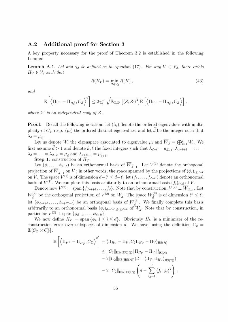
A.2 Additional proof for Section 3

A key property necessary for the proof of Theorem 3.2 is established in the followingLemma:

Lemma A.1. Let and γd be defined as in equation (17). For any V ∈ Vd, there existsHV ∈ Vd such that

R(HV ) = minH∈Vd

R(H) , (43)

and

E

[⟨ΠV ⊥ − ΠH⊥

V, CZ

⟩2]≤ 2γ−1

d

√EZ,Z′

[〈Z,Z ′〉4

]E

[⟨ΠV ⊥ − ΠH⊥

V, CZ

⟩],

where Z ′ is an independent copy of Z.

Proof. Recall the following notation: let (λi) denote the ordered eigenvalues with multi-

plicity of C1, resp. (µi) the ordered distinct eigenvalues, and let d be the integer such thatλd = µed .

Let us denote Wi the eigenspace associated to eigenvalue µi and W j =⊕j

i=1Wi. We

first assume d > 1 and denote k, ` the fixed integers such that λd−` = µed−1, λd−`+1 = . . . =λd = . . . = λd+k = µed and λd+k+1 = µed+1.

Step 1: construction of HV .Let (φ1, . . . , φd−`) be an orthonormal basis of W ed−1. Let V (1) denote the orthogonal

projection of W ed−1 on V ; in other words, the space spanned by the projections of (φi)i≤d−`

on V . The space V (1) is of dimension d−`′ ≤ d−` ; let (f1, . . . , fd−`′) denote an orthonormalbasis of V (1). We complete this basis arbitrarily to an orthonormal basis (fi)i≤d of V .

Denote now V (2) = span {fd−`+1, . . . , fd}. Note that by construction, V (2) ⊥ W ed−1. Let

W(2)ed

be the orthogonal projection of V (2) on Wed. The space W(2)ed

is of dimension `′′ ≤ ` ;

let (φd−`+1, . . . , φd+`′′−`) be an orthogonal basis of W(2)ed

. We finally complete this basis

arbitrarily to an orthonormal basis (φi)d−`+1≤i≤d+k of Wed. Note that by construction, inparticular V (2) ⊥ span {φd+1, . . . , φd+k}.

We now define HV = span {φi, 1 ≤ i ≤ d}. Obviously HV is a minimizer of the re-construction error over subspaces of dimension d. We have, using the definition C2 =E [CZ ⊗ C∗

Z ] :

E

[⟨ΠV ⊥ − ΠH⊥

V, CZ

⟩2]

= 〈ΠHV− ΠV , C2ΠHV

− ΠV 〉HS(H)

≤ ‖C2‖HS(HS(H))‖ΠHV− ΠV ‖2

HS(H)

= 2‖C2‖HS(HS(H))(d− 〈ΠV ,ΠHV〉HS(H))

= 2 ‖C2‖HS(HS(H))

(d−

d∑

i,j=1

〈fi, φj〉2)

;

36

and on the other hand, using the definition C1 = ECZ :

E

[⟨ΠV ⊥ − ΠH⊥

V, CZ

⟩]= 〈ΠHV

− ΠV , C1〉 =d∑

i=1

(λi − 〈fi, C1fi〉) .

We will decompose the last sum into two terms, for indices i smaller or greater than d− `,and bound these separately.

Step 2a: indices i ≤ d− `. In this case we decompose fi =∑

j≤d−` 〈fi, φj〉φj +gi, with

gi ∈ W⊥ed−1. We have

〈gi, C1gi〉 ≤ µed ‖gi‖2 = µed

(1 −

∑

j≤d−`

〈fi, φj〉2),

and

d−∑

i=1

(λi − 〈fi, C1fi〉) ≥d−∑

i=1

λi

(1 −

d−∑

j=1

〈fi, φj〉2)

−d−∑

i=1

µed

(1 −

∑

j≤d−`

〈fi, φj〉2)

≥(µed−1 − µed

)(d− `−

d−∑

i,j=1

〈fi, φj〉2).

Step 2b: indices i > d − `. In this case remember that fi ⊥ φj for 1 ≤ j ≤ d − `

and d + 1 ≤ j ≤ d + k. We can therefore decompose fi =∑d

j=d−`+1 〈fi, φj〉φj + g′i with

g′i ∈ W⊥ed . We have

〈g′i, C1g′i〉 ≤ µed+1 ‖g′i‖

2= µed+1

(1 −

d∑

j=d−`+1

〈fi, φj〉2),

and

d∑

i=d−`+1

(λi − 〈fi, C1fi〉) = µed

(`−

d∑

i,j=d−`+1

〈fi, φj〉2)

−d∑

i=d−`+1

〈g′i, C1g′i〉

≥(µed − µed+1

)(`−

d∑

i,j=d−`+1

〈fi, φj〉2).

Finally collecting the results of steps 2a-b we obtain

〈ΠHV− ΠV , C1〉 ≥ min

(µed−1 − µed, µed − µed+1

)(d−

d−∑

i,j=1

〈fi, φj〉2 −d∑

i,j=d−`+1

〈fi, φj〉2)

≥ min(µed−1 − µed, µed − µed+1

)(2 ‖C2‖)−1

E

[⟨ΠV ⊥ − ΠH⊥

V, CX

⟩2].

37

Finally, it holds that

‖C2‖2HS(HS(H)) = EZ,Z′

[〈CZ ⊗ C∗

Z , CZ′ ⊗ C∗Z′〉HS(HS(H))

]

= EZ,Z′

[〈CZ , CZ′〉2HS(H)

]

= EZ,Z′

[〈Z,Z ′〉4H

].

This concludes the proof of the Lemma when d > 1. If d = 1, the proof can be adaptedwith minor modifications, essentially removing step (2a), so that in the final inequalityonly the second term of the minimum appears. ¤

A.3 Proof of Theorem 4.1.

It is a well-known fact that an integral kernel operator such as Kφ is Hilbert-Schmidt ifand only if the kernel k(x, y) (here equal to 〈Φ(x),Φ(y)〉 ) is an element of L2(X × X )(endowed with the product measure) . This is the case here since k(x, y) ≤ ‖Φ(x)‖ ‖Φ(y)‖and E‖Φ(X)‖2 <∞ by assumption. We now characterize this operator more precisely.

Since E‖Φ(X)‖ < ∞, Φ(X) has an expectation which we denote by E [Φ(X)] ∈ H.Consider the linear operator T : H → L2(P ) defined as (Th)(x) = 〈h,Φ(x)〉H. By theCauchy-Schwarz inequality, E 〈h,Φ(X)〉2 ≤ ‖h‖2

E‖Φ(X)‖2. This shows that T is well-defined and continuous; therefore it has a continuous adjoint T ∗. Let f ∈ L2(P ), thenhe variable f(X)Φ(X) ∈ H has a well-defined expectation since f and ‖Φ‖ are in L2(P ).But for all g ∈ H, 〈T ∗f, g〉H = 〈f, Tg〉L2(P ) = E [〈g, f(X)Φ(X)〉H] which shows thatT ∗(f) = E [Φ(X)f(X)] .

We now show that CΦ = T ∗T and KΦ = TT ∗. By definition, for all h, h′ ∈ H,〈h, T ∗Th′〉 = 〈Th, Th′〉 = E [〈h,Φ(X)〉 〈h′,Φ(X)〉] . Thus, by the uniqueness of the covari-ance operator, we get CΦ = T ∗T. Similarly, (TT ∗f)(x) = 〈T ∗f,Φ(x)〉 = E [〈f(X)Φ(X),Φ(x)〉] =∫f(y) 〈Φ(y),Φ(x)〉 dP (y) so that KΦ = TT ∗. This also implies that KΦ is self-adjoint and

positive.We finally show that the nonzero eigenvalues of TT ∗ and T ∗T coincide by a stan-

dard argument. Let Eµ(A) = {x,Ax = µx} be the eigenspace of the operator A as-sociated with µ. Moreover, let λ > 0 be a positive eigenvalue of KΦ = TT ∗ and fan associated eigenvector. Then (T ∗T )T ∗f = T ∗(TT ∗)f = λT ∗f . This shows thatT ∗Eλ(TT

∗) ⊂ Eλ(T∗T ) ; similarly, TEλ(T

∗T ) ⊂ Eλ(TT∗). Applying T ∗ to both terms of

the last inclusion implies T ∗TEλ(T∗T ) = Eλ(T

∗T ) ⊂ T ∗Eλ(TT∗) (the first equality holds

because λ 6= 0). By the same token, Eλ(TT∗) ⊂ TEλ(T

∗T ) . Thus, Eλ(T∗T ) = T ∗Eλ(TT

∗)and Eλ(TT

∗) = TEλ(T∗T ) ; this finally implies dim(Eλ(T

∗T)) = dim(Eλ(TT∗)). Thisshows that λ is also an eigenvalue for CΦ with the same multiplicity and concludes theproof. ¤

38

B Concentration inequalities

Some concentration inequalities used all along the paper are recalled here for the sake ofcompleteness.

Theorem B.1 (McDiarmid (1989)). Let X1, . . . , Xn be n independent random variablestaking values in X and let Z = f(X1, . . . , Xn) where f is such that:

supx1,...,xn,x′

i∈X|f(x1, . . . , xn) − f(x1, . . . , x

′i, . . . , xn)| ≤ ci , ∀ 1 ≤ i ≤ n ,

thenP [Z − E [Z] ≥ ξ] ≤ e−2ξ2/(c21+...+c2n) ,

andP [E [Z] − Z ≥ ξ] ≤ e−2ξ2/(c21+...+c2n) .

Theorem B.2 (Hoeffding (1963)). Let 1 ≤ r ≤ n and X1, . . . , Xn be n independentrandom variables. Denote

U =1

n(n− 1) . . . (n− r + 1)

∑

i1 6=... 6=ir

g(Xi1 , . . . , Xir) .

If g has range in [a, b] then

P [U − E [U ] ≥ t] ≤ e−2dn/ret2/(b−a)2 ,

andP [E [U ] − U ≥ t] ≤ e−2dn/ret2/(b−a)2 .

Theorem B.3 (Bernstein’s inequality). Let f be a bounded function. With probabilityat least 1 − e−ξ,

(P − Pn)(f) ≤√

2ξPf 2

n+

‖f‖∞ξ3n

, (44)

and with probability at least 1 − e−ξ,

(Pn − P )(f) ≤√

2ξPf 2

n+

‖f‖∞ξ3n

. (45)

39