Embed Size (px)
Citation preview
Statistics and learningAn introduction: from data to modelling
Emmanuel Rachelson and Matthieu Vignes
ISAE SupAero
Wednesday 3rd September 2013
E. Rachelson & M. Vignes (ISAE) SAD 2013 1 / 13
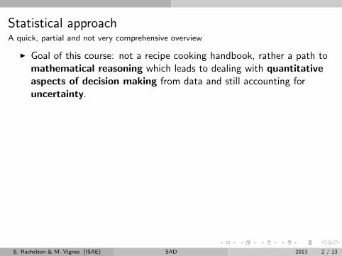
Statistical approachA quick, partial and not very comprehensive overview
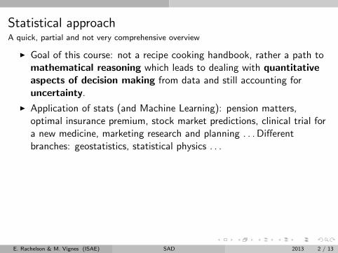
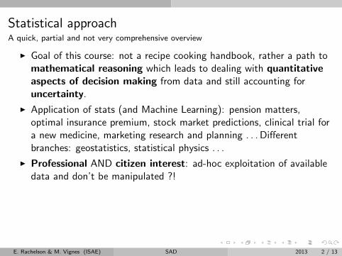
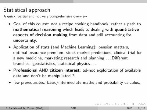
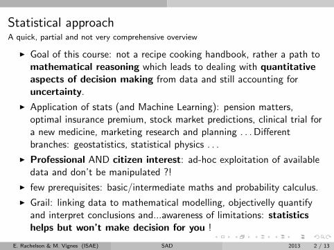
I Goal of this course: not a recipe cooking handbook, rather a path tomathematical reasoning which leads to dealing with quantitativeaspects of decision making from data and still accounting foruncertainty.
I Application of stats (and Machine Learning): pension matters,optimal insurance premium, stock market predictions, clinical trial fora new medicine, marketing research and planning . . . Differentbranches: geostatistics, statistical physics . . .
I Professional AND citizen interest: ad-hoc exploitation of availabledata and don’t be manipulated ?!
I few prerequisites: basic/intermediate maths and probability calculus.
I Grail: linking data to mathematical modelling, objectivelly quantifyand interpret conclusions and...awareness of limitations: statisticshelps but won’t make decision for you !
E. Rachelson & M. Vignes (ISAE) SAD 2013 2 / 13
Statistical approachA quick, partial and not very comprehensive overview
I Goal of this course: not a recipe cooking handbook, rather a path tomathematical reasoning which leads to dealing with quantitativeaspects of decision making from data and still accounting foruncertainty.
I Application of stats (and Machine Learning): pension matters,optimal insurance premium, stock market predictions, clinical trial fora new medicine, marketing research and planning . . . Differentbranches: geostatistics, statistical physics . . .
I Professional AND citizen interest: ad-hoc exploitation of availabledata and don’t be manipulated ?!
I few prerequisites: basic/intermediate maths and probability calculus.
I Grail: linking data to mathematical modelling, objectivelly quantifyand interpret conclusions and...awareness of limitations: statisticshelps but won’t make decision for you !
E. Rachelson & M. Vignes (ISAE) SAD 2013 2 / 13

Inspiring work / our bibliography
T. Hastie, R. Tibshirani and J. Friedman.Elements of statistical learning.Springer, 2nd edition, 2009.
E. Moulines, F. Roueff and J.-L. Pac (and
formerly F. Rossi)Statistiques.Cours TelecomParisTech, 2008.
A. Garivier
Statistiques avancees.Cours Centrale 2011, 2011.
S. Clemencon.
Apprentissage statistique.Cours TELECOM ParisTech, 2011-2012.
S. Arlot, Francis B., O. Catoni, G. Stolz and G.
ObozinskiApprentissage.Cours ENS, 2012.
N. Chopin, D. Rosenberg and G. Stolz
Elements de statistique pour citoyensd’aujourd’hui et managers de demain.Cours L3 HEC, 2012–2013.
A. Baccini, P. Besse, S. Canu, S. Dejean, B.Laurent, C. Marteau, P. Martin and H. MilhemWikistat, le cours dont vous etes le heros.http://wikistat.fr/, 2012.
A.B. Dufour D. Chessel J.R. Lobry, S. Moussetand S. DrayEnseignements de Statistique en Biologie.http://pbil.univ-lyon1.fr/R/, 2012.
F. BertrandPage professionnelle - Enseignements.http://www-irma.u-strasbg.fr/∼fbertran/
enseignement/, 2012.
V. MonbetPage professionnelle - Enseignements.http://perso.univ-rennes1.fr/valerie.monbet/
enseignement.html, 2013.
S. LousteauPage professionnelle - Enseignements.http://www.math.univ-angers.fr/ loustau/,2013.
And many others we just forgot to mention.
E. Rachelson & M. Vignes (ISAE) SAD 2013 3 / 13
From data to modellingand back
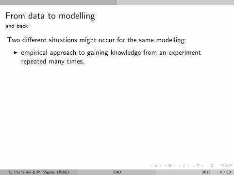
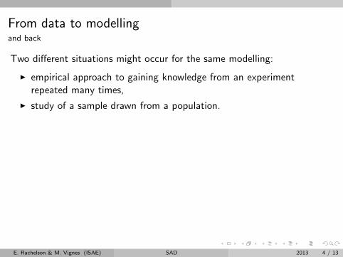
Two different situations might occur for the same modelling:
I empirical approach to gaining knowledge from an experimentrepeated many times,
I study of a sample drawn from a population.
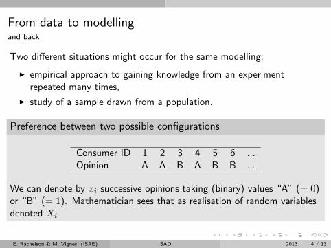
Preference between two possible configurations
Consumer ID 1 2 3 4 5 6 ...Opinion A A B A B B ...
We can denote by xi successive opinions taking (binary) values “A” (= 0)or “B” (= 1). Mathematician sees that as realisation of random variablesdenoted Xi.
E. Rachelson & M. Vignes (ISAE) SAD 2013 4 / 13
From data to modellingand back
Two different situations might occur for the same modelling:
I empirical approach to gaining knowledge from an experimentrepeated many times,
I study of a sample drawn from a population.
Preference between two possible configurations
Consumer ID 1 2 3 4 5 6 ...Opinion A A B A B B ...
We can denote by xi successive opinions taking (binary) values “A” (= 0)or “B” (= 1). Mathematician sees that as realisation of random variablesdenoted Xi.
E. Rachelson & M. Vignes (ISAE) SAD 2013 4 / 13
Localising randomness
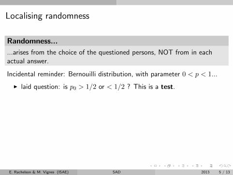
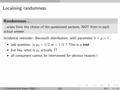
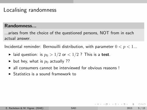
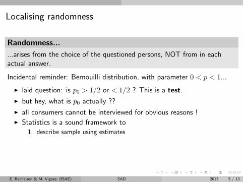
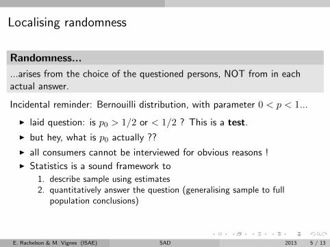
Randomness...
...arises from the choice of the questioned persons, NOT from in eachactual answer.
Incidental reminder: Bernouilli distribution, with parameter 0 < p < 1...
I laid question: is p0 > 1/2 or < 1/2 ? This is a test.
I but hey, what is p0 actually ??
I all consumers cannot be interviewed for obvious reasons !I Statistics is a sound framework to
1. describe sample using estimates2. quantitatively answer the question (generalising sample to full
population conclusions)
E. Rachelson & M. Vignes (ISAE) SAD 2013 5 / 13

Localising randomness
Randomness...
...arises from the choice of the questioned persons, NOT from in eachactual answer.
Incidental reminder: Bernouilli distribution, with parameter 0 < p < 1...
I laid question: is p0 > 1/2 or < 1/2 ? This is a test.
I but hey, what is p0 actually ??
I all consumers cannot be interviewed for obvious reasons !I Statistics is a sound framework to
1. describe sample using estimates2. quantitatively answer the question (generalising sample to full
population conclusions)
E. Rachelson & M. Vignes (ISAE) SAD 2013 5 / 13
Localising randomness
Randomness...
...arises from the choice of the questioned persons, NOT from in eachactual answer.
Incidental reminder: Bernouilli distribution, with parameter 0 < p < 1...
I laid question: is p0 > 1/2 or < 1/2 ? This is a test.
I but hey, what is p0 actually ??
I all consumers cannot be interviewed for obvious reasons !
I Statistics is a sound framework to
1. describe sample using estimates2. quantitatively answer the question (generalising sample to full
population conclusions)
E. Rachelson & M. Vignes (ISAE) SAD 2013 5 / 13
Localising randomness
Randomness...
...arises from the choice of the questioned persons, NOT from in eachactual answer.
Incidental reminder: Bernouilli distribution, with parameter 0 < p < 1...
I laid question: is p0 > 1/2 or < 1/2 ? This is a test.
I but hey, what is p0 actually ??
I all consumers cannot be interviewed for obvious reasons !I Statistics is a sound framework to
1. describe sample using estimates2. quantitatively answer the question (generalising sample to full
population conclusions)
E. Rachelson & M. Vignes (ISAE) SAD 2013 5 / 13
Localising randomness
Randomness...
...arises from the choice of the questioned persons, NOT from in eachactual answer.
Incidental reminder: Bernouilli distribution, with parameter 0 < p < 1...
I laid question: is p0 > 1/2 or < 1/2 ? This is a test.
I but hey, what is p0 actually ??
I all consumers cannot be interviewed for obvious reasons !I Statistics is a sound framework to
1. describe sample using estimates
2. quantitatively answer the question (generalising sample to fullpopulation conclusions)
E. Rachelson & M. Vignes (ISAE) SAD 2013 5 / 13
Localising randomness
Randomness...
...arises from the choice of the questioned persons, NOT from in eachactual answer.
Incidental reminder: Bernouilli distribution, with parameter 0 < p < 1...
I laid question: is p0 > 1/2 or < 1/2 ? This is a test.
I but hey, what is p0 actually ??
I all consumers cannot be interviewed for obvious reasons !I Statistics is a sound framework to
1. describe sample using estimates2. quantitatively answer the question (generalising sample to full
population conclusions)
E. Rachelson & M. Vignes (ISAE) SAD 2013 5 / 13
Modellinga mandatory step
I we start by modelling the problem (Sample/population description,variables and their distributions).
I in the example: “correct model” ∈ (Bern(p))p; n realisations (xi)i ofiid (indep. & identical. distr.) random variables (Xi)i ∼ Bern (p) areavailable.
I remember the Jean Tiberi vs. Lyne Cohen-Solal (+ Ph. Meyer)council election in Paris in 2008 between 20.45 and 21.15 ? At 20.45,(463; 409; 106) but after counting the votes :(11, 044; 11, 269; 2, 730).
I Construction of confidence intervals to answer the question.
E. Rachelson & M. Vignes (ISAE) SAD 2013 6 / 13
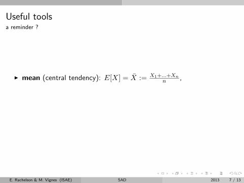
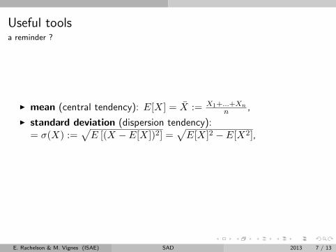
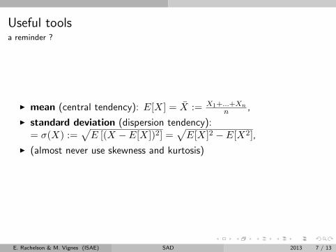
Useful toolsa reminder ?
I mean (central tendency): E[X] = X := X1+...+Xnn ,
I standard deviation (dispersion tendency):= σ(X) :=
√E [(X − E[X])2] =
√E[X]2 − E[X2],
I (almost never use skewness and kurtosis)
E. Rachelson & M. Vignes (ISAE) SAD 2013 7 / 13
Useful toolsa reminder ?
I mean (central tendency): E[X] = X := X1+...+Xnn ,
I standard deviation (dispersion tendency):= σ(X) :=
√E [(X − E[X])2] =
√E[X]2 − E[X2],
I (almost never use skewness and kurtosis)
E. Rachelson & M. Vignes (ISAE) SAD 2013 7 / 13
Useful toolsa reminder ?
I mean (central tendency): E[X] = X := X1+...+Xnn ,
I standard deviation (dispersion tendency):= σ(X) :=
√E [(X − E[X])2] =
√E[X]2 − E[X2],
I (almost never use skewness and kurtosis)
E. Rachelson & M. Vignes (ISAE) SAD 2013 7 / 13
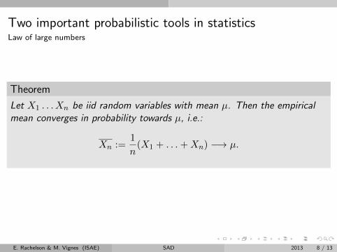
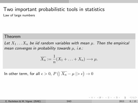
Two important probabilistic tools in statisticsLaw of large numbers
Theorem
Let X1 . . . Xn be iid random variables with mean µ. Then the empiricalmean converges in probability towards µ, i.e.:
Xn :=1
n(X1 + . . .+Xn) −→ µ.
In other term, for all ε > 0, P(| Xn − µ |> ε
)→ 0
E. Rachelson & M. Vignes (ISAE) SAD 2013 8 / 13
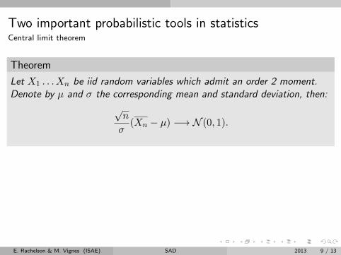
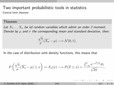
Two important probabilistic tools in statisticsCentral limit theorem
Theorem
Let X1 . . . Xn be iid random variables which admit an order 2 moment.Denote by µ and σ the corresponding mean and standard deviation, then:
√n
σ(Xn − µ) −→ N (0, 1).
In the case of distribution with density functions, this means that
P
(√n
σ(Xn − µ) ≤ x
):= Fn(x) −→ P (Z ≤ x) =
∫ x−∞ e−z
2/2 dz√
2π.
E. Rachelson & M. Vignes (ISAE) SAD 2013 9 / 13
Deciding from a sample
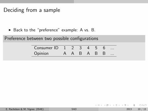
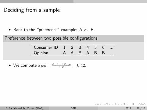
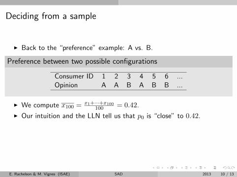
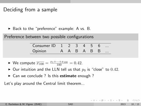
I Back to the “preference” example: A vs. B.
Preference between two possible configurations
Consumer ID 1 2 3 4 5 6 ...Opinion A A B A B B ...
I We compute x100 = x1+···+x100100 = 0.42.
I Our intuition and the LLN tell us that p0 is “close” to 0.42.
I Can we conclude ? Is this estimate enough ?
Let’s play around the Central limit theorem...
E. Rachelson & M. Vignes (ISAE) SAD 2013 10 / 13
Deciding from a sample
I Back to the “preference” example: A vs. B.
Preference between two possible configurations
Consumer ID 1 2 3 4 5 6 ...Opinion A A B A B B ...
I We compute x100 = x1+···+x100100 = 0.42.
I Our intuition and the LLN tell us that p0 is “close” to 0.42.
I Can we conclude ? Is this estimate enough ?
Let’s play around the Central limit theorem...
E. Rachelson & M. Vignes (ISAE) SAD 2013 10 / 13
Concluding the exampleat the price of a slight risk
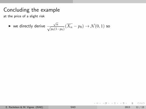
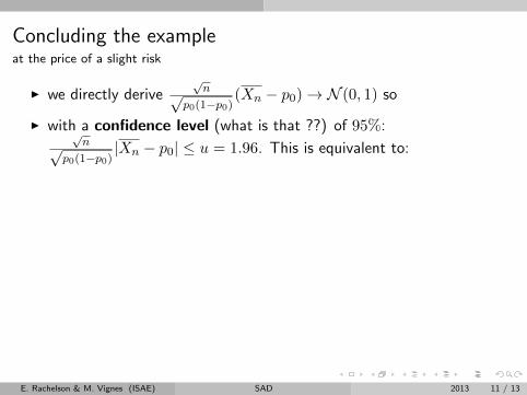
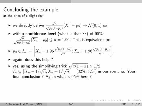
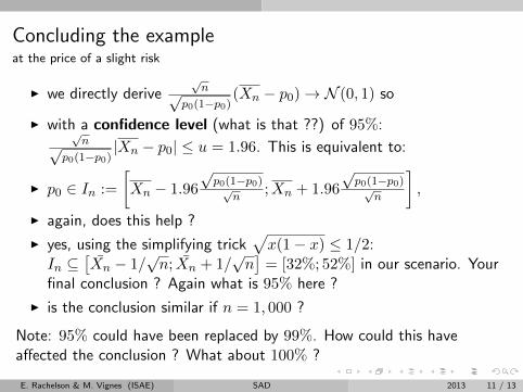
I we directly derive√n√
p0(1−p0)(Xn − p0)→ N (0, 1) so
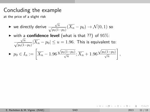
I with a confidence level (what is that ??) of 95%:√n√
p0(1−p0)|Xn − p0| ≤ u = 1.96. This is equivalent to:
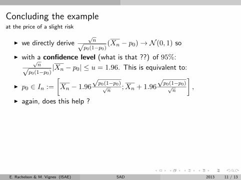
I p0 ∈ In :=
[Xn − 1.96
√p0(1−p0)√
n;Xn + 1.96
√p0(1−p0)√
n
],
I again, does this help ?
I yes, using the simplifying trick√x(1− x) ≤ 1/2:
In ⊆[Xn − 1/
√n; Xn + 1/
√n]
= [32%; 52%] in our scenario. Yourfinal conclusion ? Again what is 95% here ?
I is the conclusion similar if n = 1, 000 ?
Note: 95% could have been replaced by 99%. How could this haveaffected the conclusion ? What about 100% ?
E. Rachelson & M. Vignes (ISAE) SAD 2013 11 / 13
Concluding the exampleat the price of a slight risk
I we directly derive√n√
p0(1−p0)(Xn − p0)→ N (0, 1) so
I with a confidence level (what is that ??) of 95%:√n√
p0(1−p0)|Xn − p0| ≤ u = 1.96. This is equivalent to:
I p0 ∈ In :=
[Xn − 1.96
√p0(1−p0)√
n;Xn + 1.96
√p0(1−p0)√
n
],
I again, does this help ?
I yes, using the simplifying trick√x(1− x) ≤ 1/2:
In ⊆[Xn − 1/
√n; Xn + 1/
√n]
= [32%; 52%] in our scenario. Yourfinal conclusion ? Again what is 95% here ?
I is the conclusion similar if n = 1, 000 ?
Note: 95% could have been replaced by 99%. How could this haveaffected the conclusion ? What about 100% ?
E. Rachelson & M. Vignes (ISAE) SAD 2013 11 / 13
Hypothesis testingdecision depends on what is tested ?!
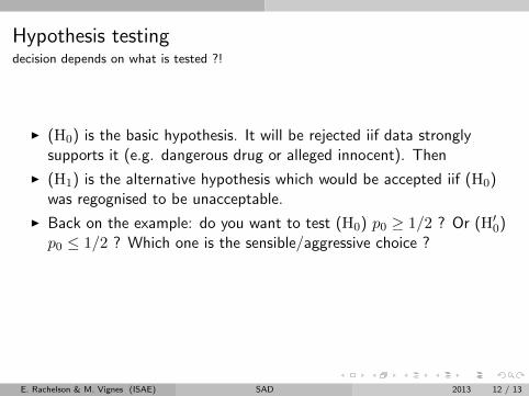
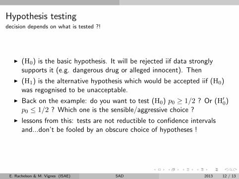
I (H0) is the basic hypothesis. It will be rejected iif data stronglysupports it (e.g. dangerous drug or alleged innocent). Then
I (H1) is the alternative hypothesis which would be accepted iif (H0)was regognised to be unacceptable.
I Back on the example: do you want to test (H0) p0 ≥ 1/2 ? Or (H′0)p0 ≤ 1/2 ? Which one is the sensible/aggressive choice ?
I lessons from this: tests are not reductible to confidence intervalsand...don’t be fooled by an obscure choice of hypotheses !
E. Rachelson & M. Vignes (ISAE) SAD 2013 12 / 13
Hypothesis testingdecision depends on what is tested ?!
I (H0) is the basic hypothesis. It will be rejected iif data stronglysupports it (e.g. dangerous drug or alleged innocent). Then
I (H1) is the alternative hypothesis which would be accepted iif (H0)was regognised to be unacceptable.
I Back on the example: do you want to test (H0) p0 ≥ 1/2 ? Or (H′0)p0 ≤ 1/2 ? Which one is the sensible/aggressive choice ?
I lessons from this: tests are not reductible to confidence intervalsand...don’t be fooled by an obscure choice of hypotheses !
E. Rachelson & M. Vignes (ISAE) SAD 2013 12 / 13
Outline of the Statistics and learning course
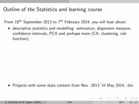
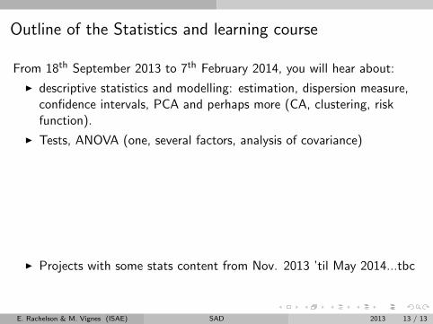
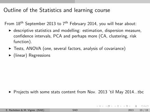
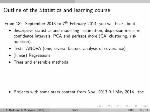
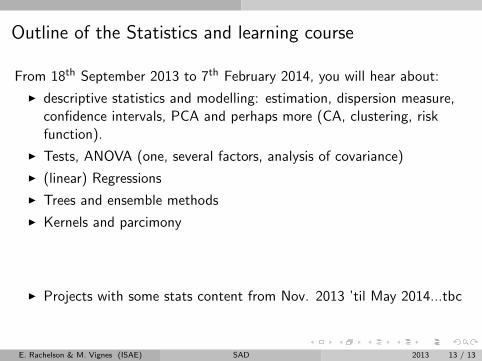
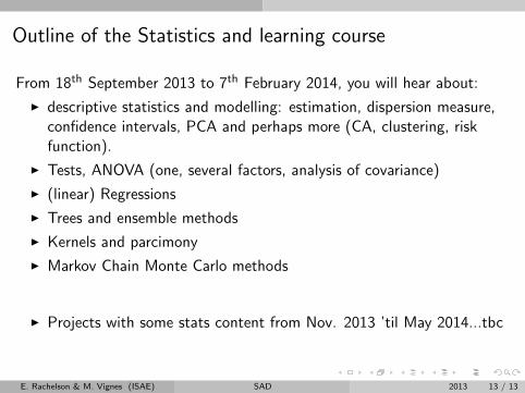
From 18th September 2013 to 7th February 2014, you will hear about:
I descriptive statistics and modelling: estimation, dispersion measure,confidence intervals, PCA and perhaps more (CA, clustering, riskfunction).
I Tests, ANOVA (one, several factors, analysis of covariance)
I (linear) Regressions
I Trees and ensemble methods
I Kernels and parcimony
I Markov Chain Monte Carlo methods
I ...and lots of R ;) !
I Projects with some stats content from Nov. 2013 ’til May 2014...tbc
E. Rachelson & M. Vignes (ISAE) SAD 2013 13 / 13
Outline of the Statistics and learning course
From 18th September 2013 to 7th February 2014, you will hear about:
I descriptive statistics and modelling: estimation, dispersion measure,confidence intervals, PCA and perhaps more (CA, clustering, riskfunction).
I Tests, ANOVA (one, several factors, analysis of covariance)
I (linear) Regressions
I Trees and ensemble methods
I Kernels and parcimony
I Markov Chain Monte Carlo methods
I ...and lots of R ;) !
I Projects with some stats content from Nov. 2013 ’til May 2014...tbc
E. Rachelson & M. Vignes (ISAE) SAD 2013 13 / 13