Statistics oflarge contact forcesin granular matter

Van Eerd, A.R.T.PhD thesis, Utrecht University, the Netherlands, September 2008With summary in DutchISBN 978-90-393-4898-7printed by Ponsen & Looijen b.v.cover designed by M.J.M. van Eerd

Statistics of large contact forces

in granular matter

Statistiek van grote contactkrachten in granulair materiaal

(met een samenvatting in het Nederlands)

Proefschrift

ter verkrijging van de graad van doctor aan de Universiteit Utrecht op gezag vande rector magnificus, prof. dr. J.C. Stoof, ingevolge het besluit van het college voorpromoties in het openbaar te verdedigen op maandag 20 oktober 2008 des middagste 2.30 uur

door

Adrianne Rudolfine Titia van Eerd

geboren op 27 november 1979 te Heesch.

Promotor Prof. dr. J.P.J.M. van der EerdenCo-promotor Dr. ir. T.J.H. Vlugt

”... en dan denk ik aan Brabant, want daar brandt nog licht.”

Guus Meeuwis, Brabant

Contents

1 Introduction 11.1 Granular materials and jamming 21.2 Studying force statistics 5

1.2.1 Experiments: boundary forces 61.2.2 Experiments: bulk forces 61.2.3 Simulations 81.2.4 Theoretical studies 9

1.3 Molecular Simulation techniques 111.3.1 Molecular Dynamics 121.3.2 Monte Carlo 141.3.3 Umbrella sampling 16

1.4 Generation of disordered packings 191.5 Force network ensemble 201.6 Umbrella sampling applied to the force network ensemble 271.7 Determination of the asymptotic behavior of P( f ) 311.8 Outline 33

2 Tail of the contact force distributions in static granular materials 352.1 Introduction 362.2 Force network ensemble and umbrella sampling 372.3 Triangular lattice 382.4 Disordered packings in two dimensions 402.5 Three- and four-dimensional packings 422.6 The effect of shear stress 452.7 Discussion 47

3 Entropy maximization in the force network ensemble for granular solids 493.1 Introduction 503.2 Force network ensemble 503.3 Entropy maximization 523.4 Results 543.5 Conclusion 64

4 Extended numerical study of the force network ensemble 674.1 Introduction 684.2 Details of the stress constraints and finite-size effects 684.3 Angle-resolved P( f ) 704.4 Maximum possible force inside a packing 774.5 Maximum shear stress of a packing 794.6 Wall versus bulk forces 834.7 Contact force distributions for systems with “real” interactions 88

References 93

Summary 103

Samenvatting 107

Curriculum vitae 113

List of publications 115

Dankwoord 117

1

Introduction

2 CHAPTER 1

1.1 Granular materials and jamming

Granular materials are systems consisting of a large number of interacting macro-scopic particles, such as sand, rice or apples, in which the range of the interactionis short compared to the particle size. These materials play an important role in ev-eryday life. A good understanding of the physics of granular materials is desired,for example, to predict and control landslides and avalanches [1, 2], to design ef-ficient transport and handling of coal or chemicals [3, 4] and to make high qualitytablets (medicine), i.e. the correct amounts of active and inert ingredients [5, 6].Unfortunately, there still remains a poor understanding of the behavior of granularmatter [7–9].

As the particles of granular materials (the grains) are larger than roughly 10 mi-crons, the thermal energy of the grains is small compared to the gravitational andelastic energy. Depending on the conditions, these athermal systems may behavelike a solid, liquid or gas. For example, sand behaves like a solid when standing onit, sand behaves like a fluid in an hourglass and sand behaves like a gas when it isshaken. The different states are in this case determined by the density and the appliedstress. Below a certain stress the system is jammed (stuck in a certain configuration)and above this stress the system is unjammed [10].

Jamming is not limited to granular materials; colloidal suspensions of small par-ticles jam as the packing density is raised and supercooled molecular liquids jam asthe temperature is lowered. Liu and Nagel have proposed that stress, packing fractionand temperature are important parameters that control jamming for all systems, andthat the state of the system can be represented by a "jamming phase diagram" [10].For the athermal granular materials, the temperature is not included in the jammingphase diagram.

A collection of grains remains easily trapped in one of the configurations thathave a local energy minimum (metastable configurations). In this thesis, we focuson the behavior of static granular materials, for which grains are packed in one ofthe many possible metastable configurations. In particular, we are interested in theforces between the grains. It is generally believed that forces between grains on themicroscopic scale are responsible for material properties at the macroscopic scale,and therefore they are worth studying. In principle there can be attractive forces be-tween grains (e.g. caused by liquid bridges), but in this study we restrict ourselves toelectrically neutral, non-magnetic grains in vacuum or air. This implies that there are

INTRODUCTION 3

0 2 4 6f

0

0.4

0.8

1.2

P(f)

τ = 0τ = 0.4

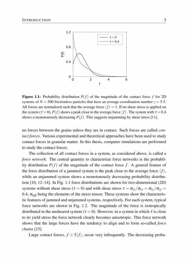
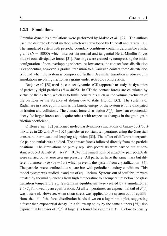
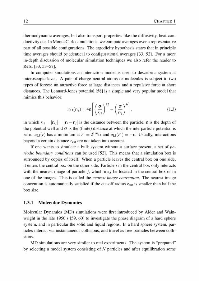
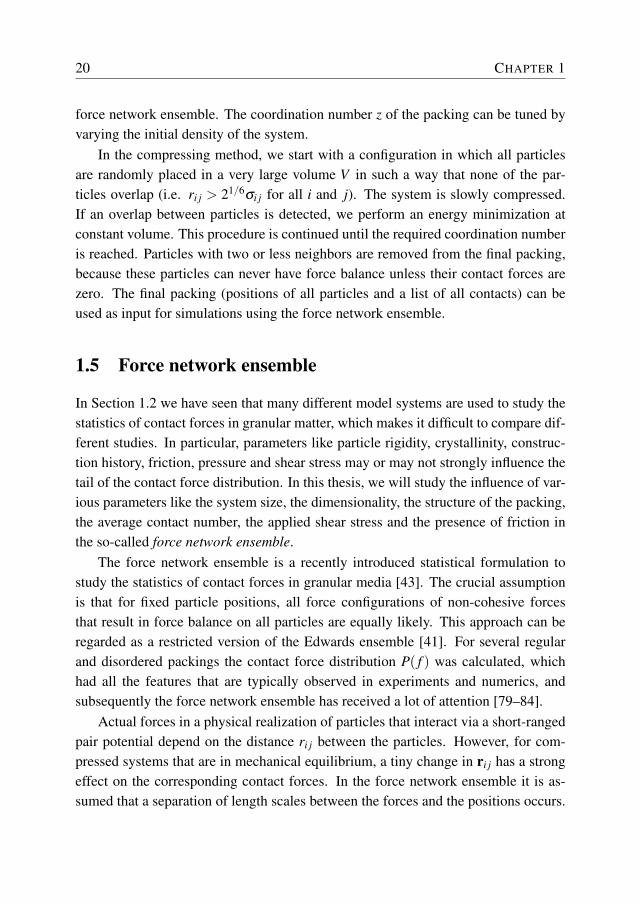
Figure 1.1: Probability distribution P( f ) of the magnitude of the contact force f for 2Dsystems of N = 500 frictionless particles that have an average coordination number z = 5.5.All forces are normalized such that the average force 〈 f 〉= 1. If no shear stress is applied onthe system (τ = 0), P( f ) shows a peak close to the average force 〈 f 〉. The system with τ = 0.4shows a monotonously decreasing P( f ). This suggests unjamming by shear stress [11].

no forces between the grains unless they are in contact. Such forces are called con-tact forces. Various experimental and theoretical approaches have been used to studycontact forces in granular matter. In this thesis, computer simulations are performedto study the contact forces.

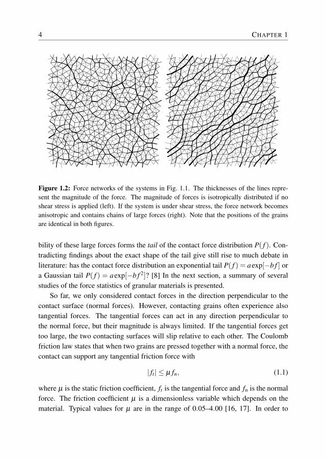
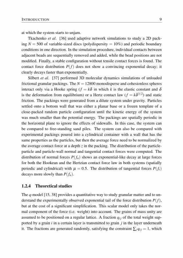
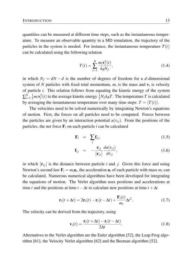
The collection of all contact forces in a system, as considered above, is called aforce network. The central quantity to characterize force networks is the probabil-ity distribution P( f ) of the magnitude of the contact force f . A general feature ofthe force distribution of a jammed system is the peak close to the average force 〈 f 〉,while an unjammed system shows a monotonously decreasing probability distribu-tion [10, 12–14]. In Fig. 1.1 force distributions are shown for two-dimensional (2D)systems without shear stress (τ = 0) and with shear stress τ = σxy/σxx = σxy/σyy =0.4, σαβ being the elements of the stress tensor. These systems show the characteris-tic features of jammed and unjammed systems, respectively. For each system, typicalforce networks are shown in Fig. 1.2. The magnitude of the force is isotropicallydistributed in the unsheared system (τ = 0). However, in a system in which τ is closeto its yield stress the force network clearly becomes anisotropic. This force networkshows that the large forces have the tendency to align and to form so-called forcechains [15].

Large contact forces, f > 5〈 f 〉, occur very infrequently. The decreasing proba-

4 CHAPTER 1

Figure 1.2: Force networks of the systems in Fig. 1.1. The thicknesses of the lines repre-sent the magnitude of the force. The magnitude of forces is isotropically distributed if noshear stress is applied (left). If the system is under shear stress, the force network becomesanisotropic and contains chains of large forces (right). Note that the positions of the grainsare identical in both figures.

bility of these large forces forms the tail of the contact force distribution P( f ). Con-tradicting findings about the exact shape of the tail give still rise to much debate inliterature: has the contact force distribution an exponential tail P( f ) = aexp[−b f ] ora Gaussian tail P( f ) = aexp[−b f 2]? [8] In the next section, a summary of severalstudies of the force statistics of granular materials is presented.

So far, we only considered contact forces in the direction perpendicular to thecontact surface (normal forces). However, contacting grains often experience alsotangential forces. The tangential forces can act in any direction perpendicular tothe normal force, but their magnitude is always limited. If the tangential forces gettoo large, the two contacting surfaces will slip relative to each other. The Coulombfriction law states that when two grains are pressed together with a normal force, thecontact can support any tangential friction force with

| ft | ≤ µ fn, (1.1)

where µ is the static friction coefficient, ft is the tangential force and fn is the normalforce. The friction coefficient µ is a dimensionless variable which depends on thematerial. Typical values for µ are in the range of 0.05–4.00 [16, 17]. In order to

INTRODUCTION 5

j

in,ij t,ij

t,ji n,ji

f

f f

f

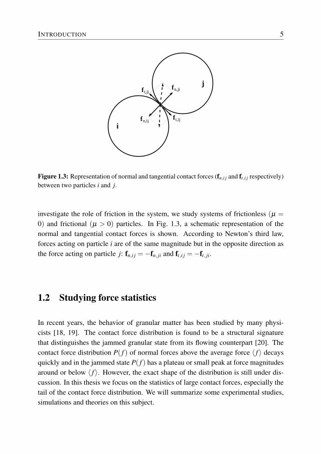
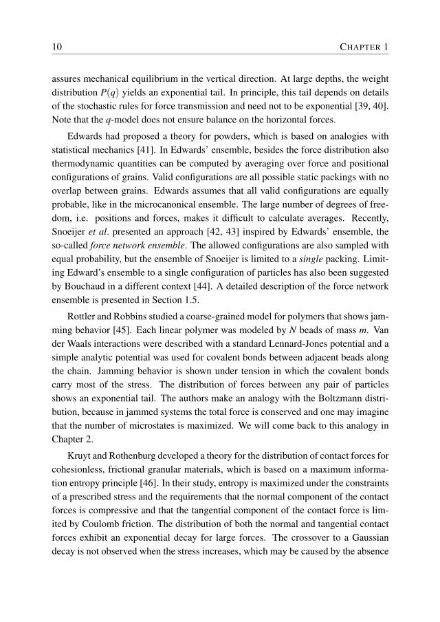
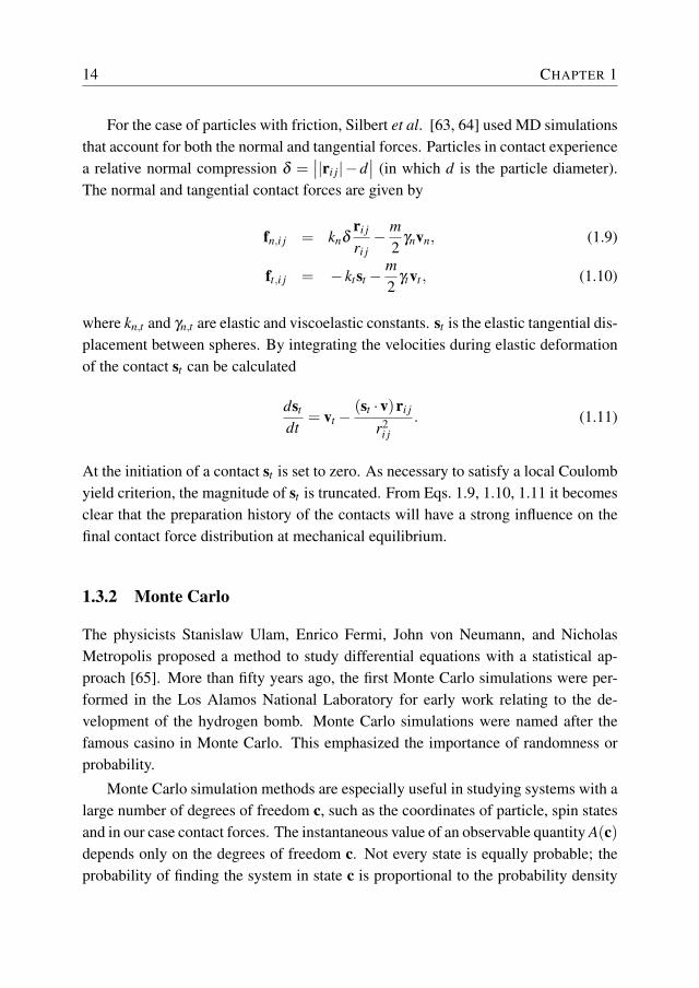
Figure 1.3: Representation of normal and tangential contact forces (fn,i j and ft,i j respectively)between two particles i and j.

investigate the role of friction in the system, we study systems of frictionless (µ =0) and frictional (µ > 0) particles. In Fig. 1.3, a schematic representation of thenormal and tangential contact forces is shown. According to Newton’s third law,forces acting on particle i are of the same magnitude but in the opposite direction asthe force acting on particle j: fn,i j =−fn, ji and ft,i j =−ft, ji.

1.2 Studying force statistics

In recent years, the behavior of granular matter has been studied by many physi-cists [18, 19]. The contact force distribution is found to be a structural signaturethat distinguishes the jammed granular state from its flowing counterpart [20]. Thecontact force distribution P( f ) of normal forces above the average force 〈 f 〉 decaysquickly and in the jammed state P( f ) has a plateau or small peak at force magnitudesaround or below 〈 f 〉. However, the exact shape of the distribution is still under dis-cussion. In this thesis we focus on the statistics of large contact forces, especially thetail of the contact force distribution. We will summarize some experimental studies,simulations and theories on this subject.

6 CHAPTER 1

1.2.1 Experiments: boundary forces

The first experiments to study contact forces in granular materials used the carbon-paper technique [15, 21–23]. The experimental setup usually contains a cylinderwith close-fitting pistons at the top and bottom surfaces. The piston at the bottom iscovered with white and carbon paper. When grains are confined in the cylinder, allbottom grains press the carbon paper into the white paper. The size and the intensityof the mark left on the white paper depend on the magnitude of the normal force onthe corresponding grain. Using image analysis software and calibration curves, thecontact forces at the surface can be extracted. Note that only boundary forces areextracted and not the forces in the bulk of the system. In these studies, the obtainedcontact force distribution P( f ) displays an exponential decay for large forces. Littleor no dependence on crystallinity, friction or deformation is observed.

Løvoll et al. [24] used an electronic balance to measure normal forces on indi-vidual grains at the bottom of a granular system without applying any external load.With this method it is possible to investigate systems which are under gravity likeregular silo systems or sand piles. The resulting P( f ) also shows an exponentialdecay.

Corwin et al. [20] measured P( f ) with a photoelastic (birefringent under strain)plate at the bottom surface of a three-dimensional (3D) cylindrical pack. This platerotates the polarization of light in proportion to the applied local pressure. The posi-tion and magnitude of the local pressure is detected by a video camera that views thetransducer through an analyzer oriented to block any unrotated light. A roughenedpiston that applies a fixed normal load to the top surface, was rotated at a constantrate. In this way, the local pressures on the bottom surface vary with time. Theboundary forces show a slower than exponential distribution for short packs (height< 20 beads) and an exponential contact force distribution for taller packs (height≥ 20 beads). The shape of this distribution does not change when a shear stress be-low the yield stress is applied. However, at the outer edge of the pack, within theshear band P( f ) exhibits markedly different behavior: the slope on a triple-log plot(see Section 1.7) is 5

3 suggesting that for large f , P( f )∼ exp[−c f 5/3].

1.2.2 Experiments: bulk forces

Majmudar et al. [25] measured the normal and tangential forces inside a 2D sys-tem of N = 2500 bidisperse photoelastic disks that were subjected to pure shear and

INTRODUCTION 7

isotropic compression. The experimental setup contains a biaxial cell with walls thatcan be moved by motorized linear slides. The cell rests horizontally on a sheet ofPlexiglas and is placed between crossed circular polarizers. From below the systemwas illuminated and from above digital images of the internal stresses were madewith a high-resolution camera. The frictional disks (µ = 0.8) are either 0.8 cm or0.9 cm in diameter with a number ratio 4:1. The sheared states were created bycompressing in one direction and expanding by an equal amount in the other direc-tion. Isotropically compressed states were created by compressing in both directions.Both systems shows a tangential force distribution P( ft) with an exponential tail. Incontrast, the normal force distribution P( fn) shows a nearly exponential tail for thesheared system and a Gaussian tail for the isotropically compressed system.

Brujic et al. [26] presented a method for measuring the contact force distributionwithin the bulk of a 3D compressed emulsion system using confocal microscopy. Thedispersed oil phase of the emulsion was fluorescently labeled and consisted of 450droplets. The emulsion droplets were compressed by an external pressure throughcentrifugation, resulting in a system which is close to the jamming transition. Thedegree of deformation, extracted from image analysis, was used to calculate the in-terdroplet normal force

f =σAR

, (1.2)

where A is the area of the deformation, σ is the interfacial tension of the droplets andR is the geometric mean of the radii of curvature of the undeformed droplets. Thelarge forces show an exponential force distribution, which is consistent with resultsof many previous experimental and simulation data on granular matter, foams andglasses [12, 22, 27, 28]. However, at large pressures, the probability distributionshows a crossover to a Gaussian-like distribution.

Zhou et al. [29] measured the interparticle contact forces inside 3D piles offrictionless liquid droplets with no Brownian motion. Three different systems werestudied: (1) a monodisperse pile, (2) a polydisperse pile subjected to its own weight,and (3) a polydisperse pile with a Teflon disk immersed in fluid on top. The dropletsurfaces were labeled with a monolayer of fluorescent nanoparticles to obtain 3Dimages with confocal fluorescence microscopy. The systems contain on the order of107 droplets; ca.103 droplets near the bottom of the piles were imaged. The contactforces were calculated with Eq. (1.2) and its probability distribution approximates aGaussian decay.

8 CHAPTER 1

1.2.3 Simulations

Granular dynamics simulations were performed by Makse et al. [27]. The authorsused the discrete element method which was developed by Cundall and Strack [30].The simulated system with periodic boundary conditions contains deformable elasticgrains (N = 10000) which interact via normal and tangential Hertz-Mindlin forcesplus viscous dissipative forces [31]. Packings were created by compressing the initialconfiguration of non-overlapping spheres. At low stress, the contact force distributionis exponential, however, a gradual transition to a Gaussian contact force distributionis found when the system is compressed further. A similar transition is observed insimulations involving frictionless grains under isotropic compression.

Radjai et al. [28] used the contact dynamics (CD) approach to study the dynamicsof perfectly rigid particles (N = 4025). In CD the contact forces are calculated byvirtue of their effect, which is to fulfill constraints such as the volume exclusion ofthe particles or the absence of sliding due to static friction [32]. The systems ofRadjai are in static equilibrium as the kinetic energy of the system is fully dissipatedin friction and collisions. The contact force distribution P( f ) shows an exponentialdecay for larger forces and is quite robust with respect to changes in the grain-grainfriction coefficient.

O’Hern et al. [12] performed molecular dynamics simulations of binary 50%/50%mixtures in 2D with N = 1024 particles at constant temperature, using the Gaussianconstraint thermostat and leapfrog algorithm [33]. The effect of different interparti-cle pair potentials was studied. The contact forces followed directly from the particlepositions. The simulations on purely repulsive potentials were carried out at con-stant reduced density ρ = N/V = 0.747; the simulations of attractive pair potentialswere carried out at zero average pressure. All particles have the same mass but dif-ferent diameters (σ2/σ1 = 1.4) which prevents the system from crystallization [34].The particles were confined to a square box with periodic boundary conditions. Thismodel system was studied in and out of equilibrium. Systems out of equilibrium werecreated by thermal quenches from high temperature to a temperature below the glasstransition temperature Tg. Systems in equilibrium were created by a simulation atT > Tg followed by an equilibration. At all temperatures, an exponential tail of P( f )was observed. However, when shear stress was applied to the system out of equilib-rium, the tail of the force distribution bends down on a logarithmic plot, suggestinga faster than exponential decay. In a follow-up study by the same authors [35], alsoexponential behavior of P( f ) at large f is found for systems at T = 0 close to density

INTRODUCTION 9

at which the system starts to unjam.Tkachenko et al. [36] used adaptive network simulations to study a 2D pack-

ing N = 500 of variable-sized discs (polydispersity = 10%) and periodic boundaryconditions in one direction. In the simulation procedure, individual contacts betweenadjacent beads are sequentially removed and added, while the bead positions are notmodified. Finally, a stable configuration without tensile contact forces is found. Thecontact force distribution P( f ) does not show a convincing exponential decay; itclearly decays faster than exponentially.

Silbert et al. [37] performed 3D molecular dynamics simulations of unloadedfrictional granular packings. The N = 12800 monodisperse and cohesionless spheresinteract only via a Hooke spring ( f = kδ in which k is the elastic constant and δ

is the deformation from equilibrium) or a Hertz contact law ( f = kδ 3/2) and staticfriction. The packings were generated from a dilute system under gravity. Particlessettled onto a bottom wall that was either a planar base or a frozen template of aclose-packed random particle configuration until the kinetic energy of the systemwas much smaller than the potential energy. The packings are spatially periodic inthe horizontal plane to ignore the effects of sidewalls. In this case, the system canbe compared to free-standing sand piles. The system can also be compared withexperimental packings poured into a cylindrical container with a wall that has thesame properties as the particles, but then the average force need to be normalized bythe average contact force at a depth z in the packing. The distribution of the particle-particle and particle-wall normal and tangential contact forces were computed. Thedistribution of normal forces P( fn) shows an exponential-like decay at large forcesfor both the Hookean and the Hertzian contact force law in both systems (spatiallyperiodic and cylindrical) with µ = 0.5. The distribution of tangential forces P( ft)decays more slowly than P( fn).

1.2.4 Theoretical studies

The q-model [15, 38] provides a quantitative way to study granular matter and to un-derstand the experimentally observed exponential tail of the force distribution P( f ),but at the cost of a significant simplification. This scalar model only takes the nor-mal component of the force (i.e. weight) into account. The grains of mass unity areassumed to be positioned on a regular lattice. A fraction qi j of the total weight sup-ported by a grain i in a certain layer is transmitted to grain j in the layer underneathit. The fractions are generated randomly, satisfying the constraint ∑i qi j = 1, which

10 CHAPTER 1

assures mechanical equilibrium in the vertical direction. At large depths, the weightdistribution P(q) yields an exponential tail. In principle, this tail depends on detailsof the stochastic rules for force transmission and need not to be exponential [39, 40].Note that the q-model does not ensure balance on the horizontal forces.

Edwards had proposed a theory for powders, which is based on analogies withstatistical mechanics [41]. In Edwards’ ensemble, besides the force distribution alsothermodynamic quantities can be computed by averaging over force and positionalconfigurations of grains. Valid configurations are all possible static packings with nooverlap between grains. Edwards assumes that all valid configurations are equallyprobable, like in the microcanonical ensemble. The large number of degrees of free-dom, i.e. positions and forces, makes it difficult to calculate averages. Recently,Snoeijer et al. presented an approach [42, 43] inspired by Edwards’ ensemble, theso-called force network ensemble. The allowed configurations are also sampled withequal probability, but the ensemble of Snoeijer is limited to a single packing. Limit-ing Edward’s ensemble to a single configuration of particles has also been suggestedby Bouchaud in a different context [44]. A detailed description of the force networkensemble is presented in Section 1.5.

Rottler and Robbins studied a coarse-grained model for polymers that shows jam-ming behavior [45]. Each linear polymer was modeled by N beads of mass m. Vander Waals interactions were described with a standard Lennard-Jones potential and asimple analytic potential was used for covalent bonds between adjacent beads alongthe chain. Jamming behavior is shown under tension in which the covalent bondscarry most of the stress. The distribution of forces between any pair of particlesshows an exponential tail. The authors make an analogy with the Boltzmann distri-bution, because in jammed systems the total force is conserved and one may imaginethat the number of microstates is maximized. We will come back to this analogy inChapter 2.

Kruyt and Rothenburg developed a theory for the distribution of contact forces forcohesionless, frictional granular materials, which is based on a maximum informa-tion entropy principle [46]. In their study, entropy is maximized under the constraintsof a prescribed stress and the requirements that the normal component of the contactforces is compressive and that the tangential component of the contact force is lim-ited by Coulomb friction. The distribution of both the normal and tangential contactforces exhibit an exponential decay for large forces. The crossover to a Gaussiandecay is not observed when the stress increases, which may be caused by the absence

INTRODUCTION 11

of kinetics that are important for elastic effects.In a series of papers [47–49], Metzger presents a very elegant model to describe

contact force statistics of force balanced grains in the isostatic limit, based on entropymaximization of the Edwards ensemble. Although an exponential tail is explicitlymentioned in Ref. [47], a closer inspection reveals that the contact force distributiondecays faster than exponential [50].

1.3 Molecular Simulation techniques

Real-life situations and experiments can often be simulated with computer models.Models used in molecular simulations contain a detailed description of the system atmicroscopic level (e.g. the atomic or molecular positions and momenta). Statisticalmechanics relates the microscopic properties to the macroscopic properties of mate-rials, such as temperature, pressure, energy and heat capacity. Computer simulationscan be used to actually compute these properties from the microscopic interactions.

Simulations are often relatively easy and cheap compared to experiments, es-pecially under extreme circumstances. Therefore, simulations can be used to studyphenomena that are not yet fully understood, such as avalanches, crystal growth orprotein folding. Although, computers are becoming faster every year, a typical simu-lation may still run for several days, weeks or even months depending on the systemsize, complexity, etc. Note that simulations have a fixed duration, meaning that only afinite number of the total number of microstates, i.e. specific microscopic configura-tions of a system, can be generated. Therefore, molecular simulations nearly alwaysprovide an estimate of a certain property.

The collection of all microstates which correspond to an identical macroscopicstate is called an ensemble. Different macroscopic environmental constraints lead todifferent types of ensembles. The following are the most important: the canonicalensemble (constant number of particles N, volume V and temperature T ), micro-canonical (constant N,V, and energy E) [51], grand-canonical (i.e., constant chemi-cal potential µ,V,T ), isobaric-isothermal, constant-stress-isothermal, and the Gibbsensemble [52].

Molecular simulation methods can roughly be divided in two categories: MonteCarlo (MC) methods and Molecular Dynamics (MD) methods. In Molecular Dy-namics, the time evolution of a system is followed by integrating the equations ofmotion. From the resulting trajectory, one can not only compute configurational or

12 CHAPTER 1

thermodynamic averages, but also transport properties like the diffusivity, heat con-ductivity etc. In Monte Carlo simulations, we compute averages over a representativepart of all possible configurations. The ergodicity hypothesis states that in principletime averages should be identical to configurational averages [33, 52]. For a morein-depth discussion of molecular simulation techniques we also refer the reader toRefs. [33, 53–57].

In computer simulations an interaction model is used to describe a system atmicroscopic level. A pair of charge neutral atoms or molecules is subject to twotypes of forces: an attractive force at large distances and a repulsive force at shortdistances. The Lennard-Jones potential [58] is a simple and very popular model thatmimics this behavior:

uLJ(ri j) = 4ε

[(σ

ri j

)12

−(

σ

ri j

)6], (1.3)

in which ri j = |ri j| = |ri− r j| is the distance between the particle, ε is the depth ofthe potential well and σ is the (finite) distance at which the interparticle potential iszero. uLJ(r) has a minimum at r∗ = 21/6σ and uLJ(r∗) = −ε . Usually, interactionsbeyond a certain distance rcut are not taken into account.

If one wants to simulate a bulk system without a surface present, a set of pe-riodic boundary conditions can be used [52]. This means that a simulation box issurrounded by copies of itself. When a particle leaves the central box on one side,it enters the central box on the other side. Particle i in the central box only interactswith the nearest image of particle j, which may be located in the central box or inone of the images. This is called the nearest image convention. The nearest imageconvention is automatically satisfied if the cut-off radius rcut is smaller than half thebox size.

1.3.1 Molecular Dynamics

Molecular Dynamics (MD) simulations were first introduced by Alder and Wain-wright in the late 1950’s [59, 60] to investigate the phase diagram of a hard spheresystem, and in particular the solid and liquid regions. In a hard sphere system, par-ticles interact via instantaneous collisions, and travel as free particles between colli-sions.

MD simulations are very similar to real experiments. The system is “prepared”by selecting a model system consisting of N particles and after equilibration some

INTRODUCTION 13

quantities can be measured at different time steps, such as the instantaneous temper-ature. To measure an observable quantity in a MD simulation, the trajectory of theparticles in the system is needed. For instance, the instantaneous temperature T (t)can be calculated using the following relation

T (t) =N

∑i=1

miv2i (t)

kBN f, (1.4)

in which N f = dN − d is the number of degrees of freedom for a d-dimensionalsystem of N particles with fixed total momentum, mi is the mass and vi is velocityof particle i. This relation follows from equating the kinetic energy of the system∑

Ni=1

12 miv2

i (t) to the average kinetic energy 12 N f kBT . The temperature T is calculated

by averaging the instantaneous temperature over many time steps: T = 〈T (t)〉.The velocities need to be solved numerically by integrating Newton’s equations

of motion. First, the forces on all particles need to be computed. Forces betweenthe particles are given by an interaction potential u(ri j). From the positions of theparticles, the net force Fi on each particle i can be calculated

Fi = ∑j

fi j, (1.5)

fi j = −ri j∣∣ri j∣∣ du(ri j)

dri j, (1.6)

in which∣∣ri j∣∣ is the distance between particle i and j. Given this force and using

Newton’s second law Fi = miai, the acceleration ai of each particle with mass mi canbe calculated. Numerous numerical algorithms have been developed for integratingthe equations of motion. The Verlet algorithm uses positions and accelerations attime t and the positions at time t−∆t to calculate new positions at time t +∆t

ri(t +∆t) = 2ri(t)− ri(t−∆t)+Fi(t)mi

∆t2. (1.7)

The velocity can be derived from the trajectory, using

vi(t) =ri(t +∆t)− ri(t−∆t)

2∆t. (1.8)

Alternatives to the Verlet algorithm are the Euler algorithm [52], the Leap Frog algo-rithm [61], the Velocity Verlet algorithm [62] and the Beeman algorithm [52].

14 CHAPTER 1

For the case of particles with friction, Silbert et al. [63, 64] used MD simulationsthat account for both the normal and tangential forces. Particles in contact experiencea relative normal compression δ =

∣∣|ri j|−d∣∣ (in which d is the particle diameter).

The normal and tangential contact forces are given by

fn,i j = knδri j

ri j− m

2γnvn, (1.9)

ft,i j = − ktst −m2

γtvt , (1.10)

where kn,t and γn,t are elastic and viscoelastic constants. st is the elastic tangential dis-placement between spheres. By integrating the velocities during elastic deformationof the contact st can be calculated

dst

dt= vt −

(st ·v)ri j

r2i j

. (1.11)

At the initiation of a contact st is set to zero. As necessary to satisfy a local Coulombyield criterion, the magnitude of st is truncated. From Eqs. 1.9, 1.10, 1.11 it becomesclear that the preparation history of the contacts will have a strong influence on thefinal contact force distribution at mechanical equilibrium.

1.3.2 Monte Carlo

The physicists Stanislaw Ulam, Enrico Fermi, John von Neumann, and NicholasMetropolis proposed a method to study differential equations with a statistical ap-proach [65]. More than fifty years ago, the first Monte Carlo simulations were per-formed in the Los Alamos National Laboratory for early work relating to the de-velopment of the hydrogen bomb. Monte Carlo simulations were named after thefamous casino in Monte Carlo. This emphasized the importance of randomness orprobability.

Monte Carlo simulation methods are especially useful in studying systems with alarge number of degrees of freedom c, such as the coordinates of particle, spin statesand in our case contact forces. The instantaneous value of an observable quantity A(c)depends only on the degrees of freedom c. Not every state is equally probable; theprobability of finding the system in state c is proportional to the probability density

INTRODUCTION 15

ρ(c). Therefore, the average of an observable A follows from

〈A〉=

∫dcρ(c)A(c)∫

dcρ(c). (1.12)

For almost all physically relevant systems, it is not possible to solve these integralsanalytically or numerically using conventional numerical integration techniques, be-cause of the high dimensional phase space of these systems. A possible way tocompute averages is to generate a sufficiently large number K of random states k.Equation (1.12) can be approximated using

〈A〉=

limK→∞

K

∑k=1

ρ(ck)A(ck)

limK→∞

K

∑k=1

ρ(ck)

. (1.13)

However, random sampling is a very inefficient approach, because almost all stateshave a very low probability density ρ(c) and will not contribute much to the nu-merator and denominator of Eq.1.13. Importance sampling solves this problem bygenerating states with a probability proportional to ρ(c). In this case, the statisti-cal weight is already taken into account in the generation of the state and thereforeensemble averages can be calculated as unweighted averages

〈A〉= limK→∞

K

∑k=1

A(ck)

K. (1.14)

This sampling scheme should not change the equilibrium distribution of the system.This is guaranteed by imposing detailed balance, which means that in equilibriumthe average number of accepted moves from the old state o to any other new state n isexactly canceled by the number of accepted reverse moves. Note that imposing strictdetailed balance is often convenient but not necessary, see Refs. [66, 67]. Metropolisdeveloped a scheme with an acceptance rule that obeys detailed balance [68]:

1. Generate an initial configuration co and calculate ρ(co).

2. Generate a new state cn by adding a random displacement to co and calculateρ(cn)

16 CHAPTER 1

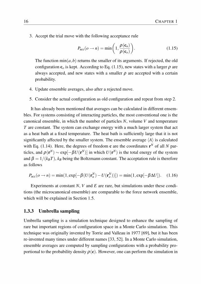
3. Accept the trial move with the following acceptance rule

Pacc(o→ n) = min(

1,ρ(cn)ρ(co)

). (1.15)

The function min(a,b) returns the smaller of its arguments. If rejected, the oldconfiguration co is kept. According to Eq. (1.15), new states with a larger ρ arealways accepted, and new states with a smaller ρ are accepted with a certainprobability.

4. Update ensemble averages, also after a rejected move.

5. Consider the actual configuration as old configuration and repeat from step 2.

It has already been mentioned that averages can be calculated in different ensem-bles. For systems consisting of interacting particles, the most conventional one is thecanonical ensemble, in which the number of particles N, volume V and temperatureT are constant. The system can exchange energy with a much larger system that actas a heat bath at a fixed temperature. The heat bath is sufficiently large that it is notsignificantly affected by the smaller system. The ensemble average 〈A〉 is calculatedwith Eq. (1.14). Here, the degrees of freedom c are the coordinates rN of all N par-ticles, and ρ(rN) ∼ exp[−βU(rN)] in which U(rN) is the total energy of the systemand β = 1/(kBT ), kB being the Boltzmann constant. The acceptation rule is thereforeas follows

Pacc(o→ n) = min(1,exp[−β (U(rNn )−U(rN

o ))]) = min(1,exp[−β∆U ]). (1.16)

Experiments at constant N, V and E are rare, but simulations under these condi-tions (the microcanonical ensemble) are comparable to the force network ensemble,which will be explained in Section 1.5.

1.3.3 Umbrella sampling

Umbrella sampling is a simulation technique designed to enhance the sampling ofrare but important regions of configuration space in a Monte Carlo simulation. Thistechnique was originally invented by Torrie and Valleau in 1977 [69], but it has beenre-invented many times under different names [33, 52]. In a Monte Carlo simulation,ensemble averages are computed by sampling configurations with a probability pro-portional to the probability density ρ(c). However, one can perform the simulation in

INTRODUCTION 17

a different ensemble (here denoted by π), in which configurations are sampled witha probability

ρ′(c) = ρ(c)exp[W (c)], (1.17)

In this equation, W (c) is an arbitrary function that only depends on c. The ensembleaverage 〈A〉π in ensemble π is defined as

〈A〉π =

∫dcA(c)ρ

′(c)∫dcρ

′(c). (1.18)

It is important to note that 〈A〉 6= 〈A〉π

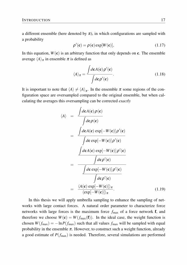
. In the ensemble π some regions of the con-figuration space are oversampled compared to the original ensemble, but when cal-culating the averages this oversampling can be corrected exactly

〈A〉 =

∫dcA(c)ρ(c)∫

dcρ(c)

=

∫dcA(c) exp[−W (c)]ρ ′(c)∫

dc exp[−W (c)]ρ ′(c)

=

∫dcA(c) exp[−W (c)]ρ ′(c)∫

dcρ′(c)∫

dc exp[−W (c)]ρ ′(c)∫dcρ

′(c)

=〈A(c) exp[−W (c)]〉π〈exp[−W (c)]〉π

. (1.19)

In this thesis we will apply umbrella sampling to enhance the sampling of net-works with large contact forces. A natural order parameter to characterize forcenetworks with large forces is the maximum force fmax of a force network f, andtherefore we choose W (c) = W ( fmax(f)). In the ideal case, the weight function ischosen W ( fmax) = − lnP( fmax) such that all values fmax will be sampled with equalprobability in the ensemble π . However, to construct such a weight function, alreadya good estimate of P( fmax) is needed. Therefore, several simulations are performed

18 CHAPTER 1

fmax

ln P

(fm

ax)

I II

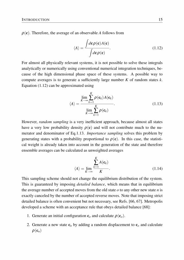
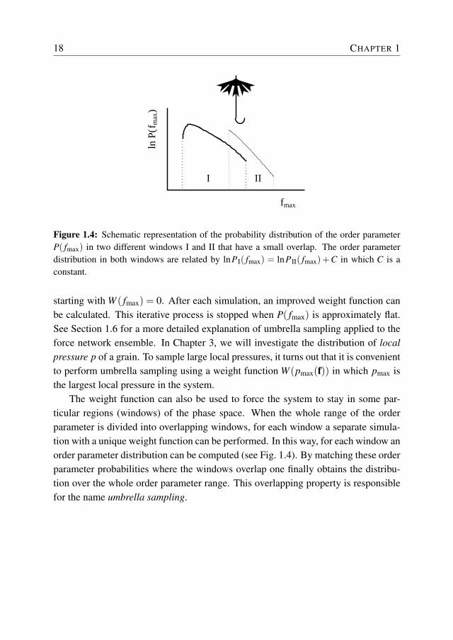
Figure 1.4: Schematic representation of the probability distribution of the order parameterP( fmax) in two different windows I and II that have a small overlap. The order parameterdistribution in both windows are related by lnPI( fmax) = lnPII( fmax) +C in which C is aconstant.

starting with W ( fmax) = 0. After each simulation, an improved weight function canbe calculated. This iterative process is stopped when P( fmax) is approximately flat.See Section 1.6 for a more detailed explanation of umbrella sampling applied to theforce network ensemble. In Chapter 3, we will investigate the distribution of localpressure p of a grain. To sample large local pressures, it turns out that it is convenientto perform umbrella sampling using a weight function W (pmax(f)) in which pmax isthe largest local pressure in the system.

The weight function can also be used to force the system to stay in some par-ticular regions (windows) of the phase space. When the whole range of the orderparameter is divided into overlapping windows, for each window a separate simula-tion with a unique weight function can be performed. In this way, for each window anorder parameter distribution can be computed (see Fig. 1.4). By matching these orderparameter probabilities where the windows overlap one finally obtains the distribu-tion over the whole order parameter range. This overlapping property is responsiblefor the name umbrella sampling.

INTRODUCTION 19

1.4 Generation of disordered packings

All numerical results presented in this thesis concern the statistics of contact forcesin static granular matter. We will investigate both positionally ordered (triangular,square, fcc and hcp lattices) and positionally disordered systems.

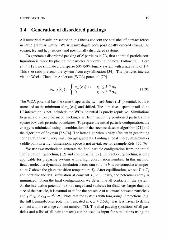
To generate a disordered packing of N particles in 2D, first an initial particle con-figuration is made by placing the particles randomly in the box. Following O’Hernet al. [12], we simulate a bidisperse 50%/50% binary system with a size ratio of 1.4.This size ratio prevents the system from crystallization [34]. The particles interactvia the Weeks-Chandler-Anderson (WCA) potential [70]

uWCA(ri j) =

{uLJ(ri j)+ ε, ri j ≤ 21/6σi j

0, ri j > 21/6σi j,(1.20)

The WCA potential has the same shape as the Lennard-Jones (LJ) potential, but it istruncated (at the minimum of uLJ(ri j)) and shifted. The attractive dispersion tail of theLJ interaction is not included: the WCA potential is purely repulsive. Simulationsto generate a force balanced packing start from randomly positioned particles in asquare box with periodic boundaries. To prepare the initial particle configuration, theenergy is minimized using a combination of the steepest descent algorithm [71] andthe algorithm of Snyman [72–74]. The latter algorithm is very efficient in generatingconfigurations with very small energy gradients. Finding a local energy minimum orsaddle point in a high-dimensional space is not trivial, see for example Refs. [75, 76].

We use two methods to generate the final particle configuration from the initialconfiguration: quenching [12] and compressing [77]. In practice, quenching is onlyapplicable for preparing systems with a high coordination number. In this method,first, a molecular dynamics simulation at constant volume V is performed at a temper-ature T above the glass transition temperature Tg. After equilibration, we set T < Tg

and continue the MD simulation at constant T , V . Finally, the potential energy isminimized. From the final configuration, we determine all contacts in the system.As the interaction potential is short-ranged and vanishes for distances larger than thesize of the particle, it is natural to define the presence of a contact between particles iand j if ri j < rcut = 21/6σi j. Note that for systems with long-range interactions (e.g.the full Lennard-Jones potential truncated at rcut ≥ 2.5σi j) it is less trivial to definecontact and the average contact number [78]. The final packing (positions of all par-ticles and a list of all pair contacts) can be used as input for simulations using the

20 CHAPTER 1

force network ensemble. The coordination number z of the packing can be tuned byvarying the initial density of the system.

In the compressing method, we start with a configuration in which all particlesare randomly placed in a very large volume V in such a way that none of the par-ticles overlap (i.e. ri j > 21/6σi j for all i and j). The system is slowly compressed.If an overlap between particles is detected, we perform an energy minimization atconstant volume. This procedure is continued until the required coordination numberis reached. Particles with two or less neighbors are removed from the final packing,because these particles can never have force balance unless their contact forces arezero. The final packing (positions of all particles and a list of all contacts) can beused as input for simulations using the force network ensemble.

1.5 Force network ensemble

In Section 1.2 we have seen that many different model systems are used to study thestatistics of contact forces in granular matter, which makes it difficult to compare dif-ferent studies. In particular, parameters like particle rigidity, crystallinity, construc-tion history, friction, pressure and shear stress may or may not strongly influence thetail of the contact force distribution. In this thesis, we will study the influence of var-ious parameters like the system size, the dimensionality, the structure of the packing,the average contact number, the applied shear stress and the presence of friction inthe so-called force network ensemble.

The force network ensemble is a recently introduced statistical formulation tostudy the statistics of contact forces in granular media [43]. The crucial assumptionis that for fixed particle positions, all force configurations of non-cohesive forcesthat result in force balance on all particles are equally likely. This approach can beregarded as a restricted version of the Edwards ensemble [41]. For several regularand disordered packings the contact force distribution P( f ) was calculated, whichhad all the features that are typically observed in experiments and numerics, andsubsequently the force network ensemble has received a lot of attention [79–84].

Actual forces in a physical realization of particles that interact via a short-rangedpair potential depend on the distance ri j between the particles. However, for com-pressed systems that are in mechanical equilibrium, a tiny change in ri j has a strongeffect on the corresponding contact forces. In the force network ensemble it is as-sumed that a separation of length scales between the forces and the positions occurs.

INTRODUCTION 21

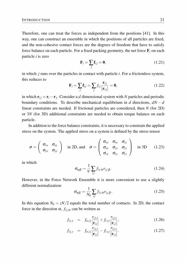
Therefore, one can treat the forces as independent from the positions [41]. In thisway, one can construct an ensemble in which the positions of all particles are fixed,and the non-cohesive contact forces are the degrees of freedom that have to satisfyforce balance on each particle. For a fixed packing geometry, the net force Fi on eachparticle i is zero

Fi = ∑j

fi j = 0, (1.21)

in which j runs over the particles in contact with particle i. For a frictionless system,this reduces to

Fi = ∑j

fi j = ∑j

fi jri j∣∣ri j∣∣ = 0, (1.22)

in which ri j = ri−r j. Consider a d dimensional system with N particles and periodicboundary conditions. To describe mechanical equilibrium in d directions, dN − dlinear constraints are needed. If frictional particles are considered, then N (for 2D)or 3N (for 3D) additional constraints are needed to obtain torque balance on eachparticle.

In addition to the force balance constraints, it is necessary to constrain the appliedstress on the system. The applied stress on a system is defined by the stress tensor

σ =

(σxx σxy

σyx σyy

)in 2D, and σ =

σxx σxy σxz

σyx σyy σyz

σzx σzy σzz

in 3D (1.23)

in whichσαβ ∼

1V ∑

i jfi j,αri j,β . (1.24)

However, in the Force Network Ensemble it is more convenient to use a slightlydifferent normalization:

σαβ =1

Nb∑i j

fi j,αri j,β . (1.25)

In this equation Nb = zN/2 equals the total number of contacts. In 2D, the contactforce in the direction α , fi j,α can be written as

fi j,x = fn,i jri j,x∣∣ri j∣∣ + ft,i j

ri j,y∣∣ri j∣∣ , (1.26)

fi j,y = fn,i jri j,y∣∣ri j∣∣ − ft,i j

ri j,x∣∣ri j∣∣ . (1.27)

22 CHAPTER 1

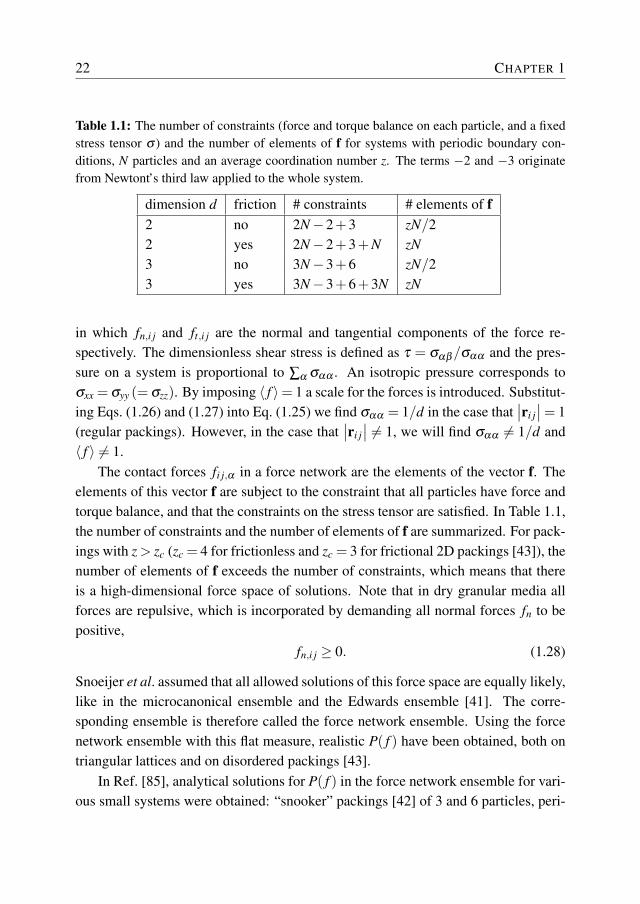
Table 1.1: The number of constraints (force and torque balance on each particle, and a fixedstress tensor σ ) and the number of elements of f for systems with periodic boundary con-ditions, N particles and an average coordination number z. The terms −2 and −3 originatefrom Newtont’s third law applied to the whole system.

dimension d friction # constraints # elements of f2 no 2N−2+3 zN/22 yes 2N−2+3+N zN3 no 3N−3+6 zN/23 yes 3N−3+6+3N zN

in which fn,i j and ft,i j are the normal and tangential components of the force re-spectively. The dimensionless shear stress is defined as τ = σαβ /σαα and the pres-sure on a system is proportional to ∑α σαα . An isotropic pressure corresponds toσxx = σyy (= σzz). By imposing 〈 f 〉= 1 a scale for the forces is introduced. Substitut-ing Eqs. (1.26) and (1.27) into Eq. (1.25) we find σαα = 1/d in the case that

∣∣ri j∣∣= 1

(regular packings). However, in the case that∣∣ri j∣∣ 6= 1, we will find σαα 6= 1/d and

〈 f 〉 6= 1.The contact forces fi j,α in a force network are the elements of the vector f. The

elements of this vector f are subject to the constraint that all particles have force andtorque balance, and that the constraints on the stress tensor are satisfied. In Table 1.1,the number of constraints and the number of elements of f are summarized. For pack-ings with z > zc (zc = 4 for frictionless and zc = 3 for frictional 2D packings [43]), thenumber of elements of f exceeds the number of constraints, which means that thereis a high-dimensional force space of solutions. Note that in dry granular media allforces are repulsive, which is incorporated by demanding all normal forces fn to bepositive,

fn,i j ≥ 0. (1.28)

Snoeijer et al. assumed that all allowed solutions of this force space are equally likely,like in the microcanonical ensemble and the Edwards ensemble [41]. The corre-sponding ensemble is therefore called the force network ensemble. Using the forcenetwork ensemble with this flat measure, realistic P( f ) have been obtained, both ontriangular lattices and on disordered packings [43].

In Ref. [85], analytical solutions for P( f ) in the force network ensemble for vari-ous small systems were obtained: “snooker” packings [42] of 3 and 6 particles, peri-

INTRODUCTION 23

odic triangular lattices of 2×2 and 3×3, and a periodic fcc unit cell (8 particles). InRef. [80] analytical expressions are derived for both isotropic and anisotropic forcedistributions in the 3×3 triangular lattice. Unfortunately, these analytical approachesare not suited for larger systems so we have to rely on computer simulations. To com-pute a single solution of the force space of a disordered system, a simulated annealingprocedure can be applied [71]. For arbitrary forces, a penalty function U(f) is definedthat describes the deviation from the required constraints. For a 2D frictionless sys-tem with

∣∣ri j∣∣= 1, this penalty function is defined as

U(f) = |σxy(f)−σreqxy | + |σxx(f)− 1

2 | + |σyy(f)− 12 |

+N

∑i=1|Fi,x(f)| +

N

∑i=1|Fi,y(f)|. (1.29)

in which σreqxy is the required (imposed) shear stress of the system. The following

Monte Carlo procedure can be used to generate a single force network f that obeysthe required constraints

1. Start with a configuration fold in which all forces are taken from an arbitrarydistribution with 〈 f 〉= 1 and fi j ≥ 0. Set the control parameter β = 1 (equiv-alent to the temperature) and calculate the penalty function U(fold).

2. Select two elements (contact forces) of f at random.

3. Add a randomly selected ∆ f to one contact force and −∆ f to the other contactforce, so that 〈 f 〉 still equals 1. If any of these forces becomes smaller than 0,the move is rejected and we return to step 2.

4. Calculate the penalty function U(fnew).

5. Accept the trial move with the acceptance rule Eq. (1.16). If rejected, the oldconfiguration is kept.

6. Increase β by multiplying with a factor h > 1 (i.e. annealing).

7. Return to step 2 until the penalty function is very small (typically 10−12). Theresulting f is considered as a particular solution of the force network ensemble.

It is trivial to extend this scheme for frictional packings and packings with∣∣ri j∣∣ 6= 1.

In previous studies [11, 43, 85, 86], the solution space of the force network ensemble

24 CHAPTER 1

was sampled by generating many particular solutions obtained using this simulatedannealing scheme. This scheme reproduces analytic results for small regular pack-ings very well [85] and it was verified that the results do not depend on the initialconfigurations and details of the annealing scheme. Unfortunately, this simulatedannealing procedure is computationally expensive and it cannot be guaranteed thatforce networks are indeed generated with equal a priori probability. Moreover, accu-rate statistics for large contact forces can not be obtained directly.

At this point it is important to note that the force network ensemble can be for-mulated as an inhomogeneous matrix equation

A f = b, (1.30)

in which static force (and torque) balance on each particle as well as a conservedstress tensor are incorporated [43]. The elements of the fixed matrix A are deter-mined by the geometry of the packing. The vector b reflects the force and torquebalance on each grain, as well as the fixed stress tensor. For a 2D system, b =(0,0, · · · ,0,σxx,σyy,σxy). All possible solutions of Eq. (1.30) can be written as

f = f0 +∑k

akvk, (1.31)

where f0 is a particular solution and the vectors vk span the null-space of matrix A ,i.e.,

A vk = 0. (1.32)

The number of independent null vectors follows directly from Table 1.1. The coeffi-cients ak are restricted by the condition that all elements of f corresponding to normalforces need to be positive. For disordered packings, we used the simulated annealingprocedure described earlier to obtain both a particular solution f0 and the null vectorsvk. Note that in order to compute a null-vector, the penalty function has to be mod-ified slightly and one needs to realize that the elements of vk can be positive as wellas negative. All vectors of the null-space are orthogonalized for efficiency reasons ofour sampling scheme, although in principle this is not needed for the correctness ofour scheme.

The force network ensemble is sampled by the usual Metropolis Monte Carlotechnique (see Section 1.3.2) in which the coefficients ak are the degrees of freedom.The Monte Carlo scheme is started with ak = 0 and a particular solution f0. In atrial move, a coefficient ak is chosen at random and its value is changed randomly.

INTRODUCTION 25

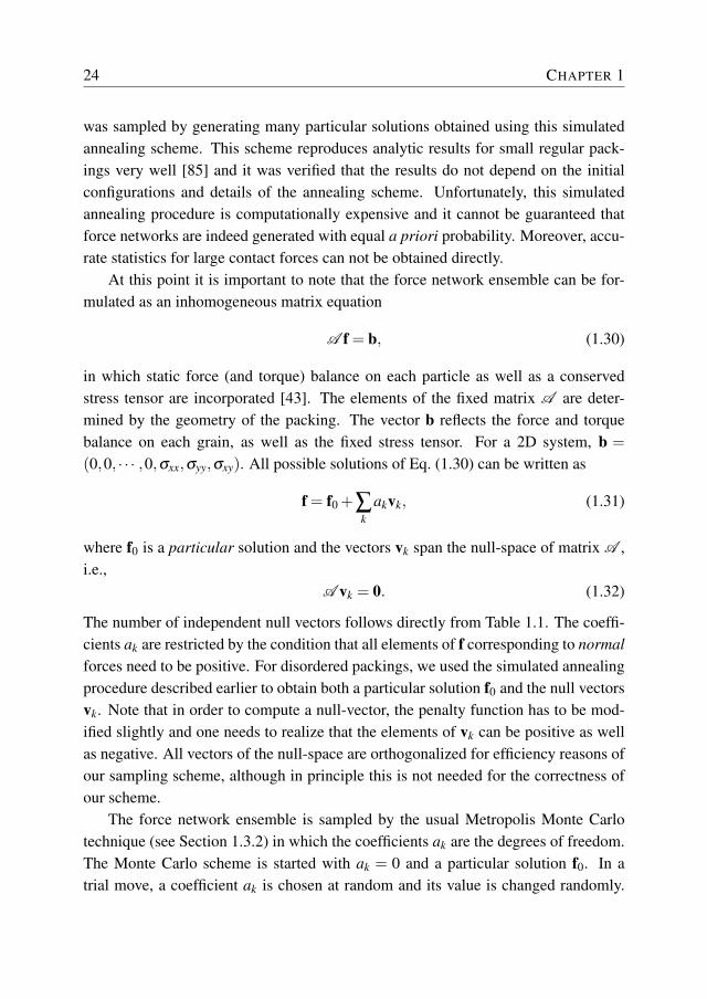
Figure 1.5: Sampling force networks of a frictionless triangular lattice [80]. The thicknessof the lines represent the magnitude of the (normal) force. In the starting configuration (left)all normal contact forces are equal to 1. After a wheel move, 6 normal forces (the “rim”) getdisplacement of +∆ and six other forces (the “spokes”) get a displacement of −∆. This newconfiguration (right) still satisfies force balance on each particle and the stress tensor doesnot change. If any of the contact forces will become smaller than zero, the wheel move isrejected.

A trial move is accepted when all normal forces fi j ≥ 0. For frictional systems, onehas to take into account the Coulomb criterium Eq. 1.1 in the acceptance rule. Inthis scheme, it is guaranteed that all allowed force networks are sampled with equalprobability.

For the triangular, square, and fcc lattice, it is convenient to choose f0 such thatall elements f0 are all equal to 1. The null-space vk can be expressed by the so-called “wheel moves” developed by Tighe et al. [80]. For a frictionless triangularlattice, a wheel move is centered around a single particle. As can be seen in Fig. 1.5,only 12 forces are involved in a wheel move: 6 contact forces of the central particle(“spokes”) and six forces that form the “rim” of the central particle. Therefore, all el-ements of vk are equal to zero except these 12 forces. In the MC procedure describedabove, the forces of the rim get a displacement of +∆ and the spokes get a displace-ment of −∆. The obtained configuration still satisfies the required constraints. Theadvantage of a local wheel move is the low number of forces that are changed. Thismeans that a larger maximum displacement ∆ is allowed. B.P. Tighe has developeda set of (local) wheel moves for the frictionless triangular lattice, the frictionless fcclattice, the frictional triangular lattice, and the frictional square lattice [87].

In previous simulations in the force network ensemble for disordered systems [11,40, 43, 85, 86], the value of all bond lengths

∣∣ri j∣∣ in Eqs. (1.26) and (1.27) was

simply set to 1, even for contacts at a distance not equal to 1. Essentially, this

26 CHAPTER 1

(a)0 1 2 3 4

f

0

0.5

1

1.5P(

f)

FASAmatrix, |rij| = 1matrix, |rij| ≠ 1

(b)0 1 2 3 4 5

f

10−6

10−4

10−2

100

P(f)

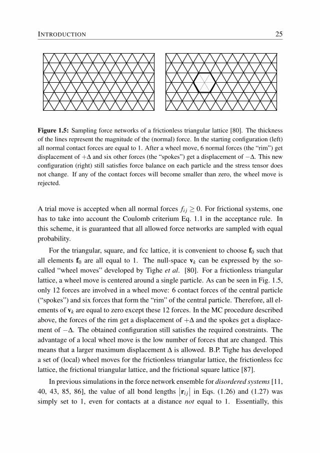
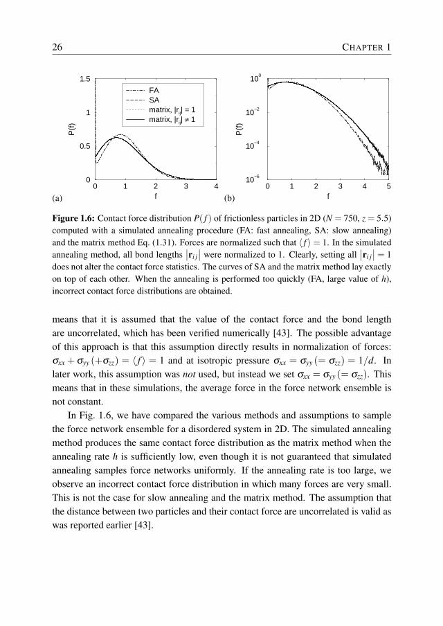
Figure 1.6: Contact force distribution P( f ) of frictionless particles in 2D (N = 750, z = 5.5)computed with a simulated annealing procedure (FA: fast annealing, SA: slow annealing)and the matrix method Eq. (1.31). Forces are normalized such that 〈 f 〉= 1. In the simulatedannealing method, all bond lengths

∣∣ri j∣∣ were normalized to 1. Clearly, setting all

∣∣ri j∣∣ = 1

does not alter the contact force statistics. The curves of SA and the matrix method lay exactlyon top of each other. When the annealing is performed too quickly (FA, large value of h),incorrect contact force distributions are obtained.

means that it is assumed that the value of the contact force and the bond lengthare uncorrelated, which has been verified numerically [43]. The possible advantageof this approach is that this assumption directly results in normalization of forces:σxx + σyy (+σzz) = 〈 f 〉 = 1 and at isotropic pressure σxx = σyy (= σzz) = 1/d. Inlater work, this assumption was not used, but instead we set σxx = σyy (= σzz). Thismeans that in these simulations, the average force in the force network ensemble isnot constant.

In Fig. 1.6, we have compared the various methods and assumptions to samplethe force network ensemble for a disordered system in 2D. The simulated annealingmethod produces the same contact force distribution as the matrix method when theannealing rate h is sufficiently low, even though it is not guaranteed that simulatedannealing samples force networks uniformly. If the annealing rate is too large, weobserve an incorrect contact force distribution in which many forces are very small.This is not the case for slow annealing and the matrix method. The assumption thatthe distance between two particles and their contact force are uncorrelated is valid aswas reported earlier [43].

INTRODUCTION 27

1.6 Umbrella sampling applied to the force networkensemble

In Section 1.5, we have shown how to sample all solutions of the force networkensemble using a Monte Carlo scheme. The sampling is performed in the spacespanned by the null-vectors of matrix A (see Eq. (1.31)). All force networks forwhich all elements of f are positive are in principle equally likely. However, thenumber of force networks in which at least one of the forces is much larger than theaverage force is low compared to force networks in which all forces are quite close tothe average force. Therefore, standard Monte Carlo sampling results in poor statisticsfor the tail of the contact force distribution P( f ). As explained in Section 1.3.3,this can be improved using umbrella sampling. To improve the statistics for largecontact forces, we use the largest force of a certain force network fmax(f) as an orderparameter. The probability density in the modified ensemble then becomes

ρ′(f) = ρ(f)exp[W ( fmax(f))], (1.33)

in which ρ(f) is the statistical weight of the force network ensemble and W ( fmax(f))is a weight function. Ensemble averages in the force network ensemble can be com-puted using

〈A〉=〈A(f) exp[−W ( fmax(f))]〉π〈exp[−W ( fmax(f))]〉π

, (1.34)

in which we used the shorthand 〈· · · 〉π

to compute averages in the modified ensemble.For example, the probability distribution of the largest force in the system can becomputed from

P( fmax) =

∫dfρ(f)δ ( fmax− f ′max(f))∫

dfρ(f)

=Pπ( fmax) exp[−W ( fmax)]∫

d f ′max Pπ( f ′max) exp[−W ( f ′max)], (1.35)

in which Pπ(· · ·) denotes a probability distribution in the modified ensemble. Notethat the probability distribution P( fmax) will depend on the size of the system. Simi-

28 CHAPTER 1

larly, we can write for the contact force distribution

P( f ) = lima→∞

∫ a

0d fmax P( f | fmax)P( fmax)∫ a

0d f ′

∫ a

0d fmax P( f ′| fmax)P( fmax)

, (1.36)

in which P( f | fmax) is the conditional contact force distribution given that the maxi-mum force in the force network equals fmax. Of course, P( f | fmax) = 0 if f > fmax.The distribution P( f | fmax) can be computed directly in a simulation in the modifiedensemble.

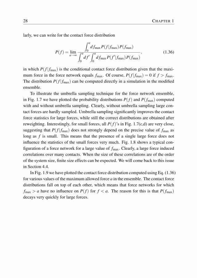
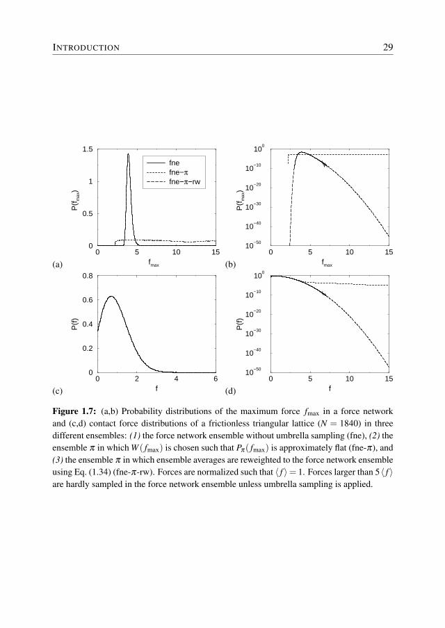
To illustrate the umbrella sampling technique for the force network ensemble,in Fig. 1.7 we have plotted the probability distributions P( f ) and P( fmax) computedwith and without umbrella sampling. Clearly, without umbrella sampling large con-tact forces are hardly sampled. Umbrella sampling significantly improves the contactforce statistics for large forces, while still the correct distributions are obtained afterreweighting. Interestingly, for small forces, all P( f )’s in Fig. 1.7(c,d) are very close,suggesting that P( f | fmax) does not strongly depend on the precise value of fmax aslong as f is small. This means that the presence of a single large force does notinfluence the statistics of the small forces very much. Fig. 1.8 shows a typical con-figuration of a force network for a large value of fmax. Clearly, a large force inducedcorrelations over many contacts. When the size of these correlations are of the orderof the system size, finite size effects can be expected. We will come back to this issuein Section 4.4.

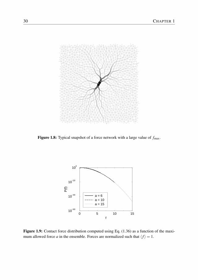
In Fig. 1.9 we have plotted the contact force distribution computed using Eq. (1.36)for various values of the maximum allowed force a in the ensemble. The contact forcedistributions fall on top of each other, which means that force networks for whichfmax > a have no influence on P( f ) for f < a. The reason for this is that P( fmax)decays very quickly for large forces.

INTRODUCTION 29

(a)0 5 10 15

fmax

0

0.5

1

1.5

P(f m

ax)

fnefne−πfne−π−rw

(b)0 5 10 15

fmax

10−50

10−40

10−30

10−20

10−10

100

P(f

max

)

(c)0 2 4 6

f

0

0.2

0.4

0.6

0.8

P(f

)

(d)0 5 10 15

f

10−50

10−40

10−30

10−20

10−10

100

P(f

)

Figure 1.7: (a,b) Probability distributions of the maximum force fmax in a force networkand (c,d) contact force distributions of a frictionless triangular lattice (N = 1840) in threedifferent ensembles: (1) the force network ensemble without umbrella sampling (fne), (2) theensemble π in which W ( fmax) is chosen such that Pπ( fmax) is approximately flat (fne-π), and(3) the ensemble π in which ensemble averages are reweighted to the force network ensembleusing Eq. (1.34) (fne-π-rw). Forces are normalized such that 〈 f 〉= 1. Forces larger than 5〈 f 〉are hardly sampled in the force network ensemble unless umbrella sampling is applied.

30 CHAPTER 1

Figure 1.8: Typical snapshot of a force network with a large value of fmax.

0 5 10 15f

10−60

10−40

10−20

100

P(f

)

a = 6a = 10a = 15

Figure 1.9: Contact force distribution computed using Eq. (1.36) as a function of the maxi-mum allowed force a in the ensemble. Forces are normalized such that 〈 f 〉= 1.

INTRODUCTION 31

1.7 Determination of the asymptotic behavior of P( f )

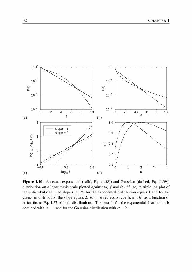
In Chapter 2 we will see that for very large contact forces, the asymptotic behavior(the “tail”) of contact force distributions can be described by

P( f )∼ aexp[−b f α ]. (1.37)

In particular, it is interesting to see whether this distribution is exponential (α = 1),Gaussian (α = 2), or something else. We considered two options to extract α:

1. The use of a triple-log plot, i.e. a plot of log10(− log10 P( f )) versus log10 f . Ingood approximation the slope of such a plot will equal α .

2. For f �〈 f 〉, we perform linear regression to fit a and b in log10 P( f ) = a−b f α

for a wide range of α . The maximum in the regression coefficient R2 is usedto determine α .

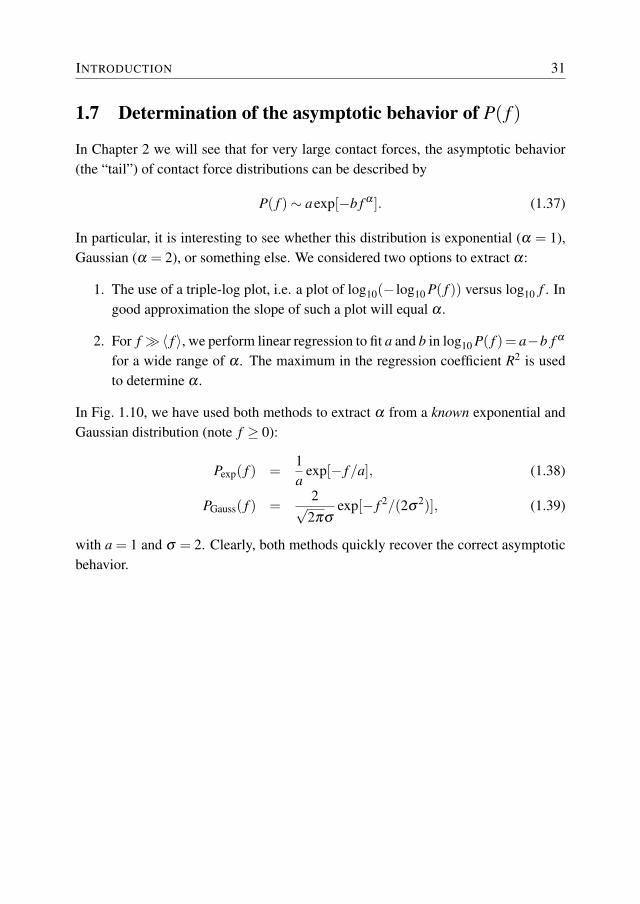
In Fig. 1.10, we have used both methods to extract α from a known exponential andGaussian distribution (note f ≥ 0):

Pexp( f ) =1a

exp[− f /a], (1.38)

PGauss( f ) =2√

2πσexp[− f 2/(2σ

2)], (1.39)

with a = 1 and σ = 2. Clearly, both methods quickly recover the correct asymptoticbehavior.

32 CHAPTER 1

(a)0 2 4 6 8 10

f

10−6

10−4

10−2

100

P(f

)

(b)0 20 40 60 80 100

f2

10−6

10−4

10−2

100

P(f

)

(c)−0.5 0.5 1.5

log10 f

−1

0

1

2

log 10

(−lo

g 10 P

(f))

slope = 1slope = 2

(d)0 1 2 3 4

α

0.6

0.7

0.8

0.9

1.0

R2

Figure 1.10: An exact exponential (solid, Eq. (1.38)) and Gaussian (dashed, Eq. (1.39))distribution on a logarithmic scale plotted against (a) f and (b) f 2. (c) A triple-log plot ofthese distributions. The slope (i.e. α) for the exponential distribution equals 1 and for theGaussian distribution the slope equals 2. (d) The regression coefficient R2 as a function ofα for fits to Eq. 1.37 of both distributions. The best fit for the exponential distribution isobtained with α = 1 and for the Gaussian distribution with α = 2.

INTRODUCTION 33

1.8 Outline

This thesis focuses on the statistics of large forces in granular media by using theforce network ensemble. One of the crucial questions is whether the tail of the contactforce distribution P( f ) is exponential, Gaussian, or even some other form. We resortto umbrella sampling to unambiguously resolve the asymptotic decay of P( f ) forlarge f , and determine P( f ) down to values of order 10−45.

In Chapter 2, we study the distribution P( f ) of contact forces between friction-less particles. We explore the effect of packing structure, dimensionality, systemsize, contact number and shear stress. We find that local force balance constraintsdetermine the asymptotic behavior of P( f ) and that the dimensionality is the mostimportant parameter that determines the tail of P( f ). In particular, we find that P( f )decays as aexp[−b f α ] with α = 2.0±0.1 for 2D systems, α = 1.7±0.1 for 3D sys-tems and α = 1.4±0.1 for 4D systems. Other factors like the coordination numberand the structure of the packing are of less importance.

Chapter 3 presents simulations of the local pressure distribution for both friction-less and frictional packings. The numerically obtained pressure distributions are inexcellent agreement with the pressure distributions obtained from an entropy maxi-mization argument by B.P. Tighe et al. [88]. The latter follows from a previouslynot exploited conserved quantity in the force network ensemble: the total area of theso-called reciprocal tiling, which follows directly from force balance on each particle.

Finally, in Chapter 4 we present a detailed study on the force network ensemblefor various packings/systems. In particular, we focus on dimensionality of the forcespace, the maximum possible force of a packing, the effect of boundary forces, andthe angle-resolved contact force distribution. We also present a comparison of thecontact force statistics between the force network ensemble and packings of particlesthat interact with a real pair potential.

2

Tail of the contact force distributions instatic granular materials

We numerically study the distribution P( f ) of contact forces in frictionless beadpacks, by averaging over the ensemble of all possible force network configurations.We resort to umbrella sampling to resolve the asymptotic decay of P( f ) for large f ,and determine P( f ) down to values of order 10−45 for ordered and disordered sys-tems in two (2D) and three dimensions (3D). Our findings unambiguously show that,in the ensemble approach, the force distributions decay much faster than exponen-tially: P( f ) ∼ exp(−c f α), with α ≈ 2.0 for 2D systems, α ≈ 1.7 for 3D systems,and α ≈ 1.4 for 4D systems.

This chapter is for a large part based on:A.R.T. van Eerd, W.G. Ellenbroek, M. van Hecke, J.H. Snoeijer, and T.J.H. VlugtTail of the contact force distribution in static granular materialsPhys. Rev. E 75, 060302 (2007)

36 CHAPTER 2

2.1 Introduction

The contact forces inside a static packing of grains are organized into highly het-erogeneous force networks, and can be characterized by the probability density ofcontact forces P( f ) [18]. Such force statistics were first studied in a series of exper-iments that measured forces through imprints on carbon paper at the boundaries of agranular assembly. Unexpectedly, the obtained P( f ) displayed an exponential ratherthan a Gaussian decay for large forces [15, 21–23]. After these initial findings, otherexperimental techniques have revealed similarly exponentially decaying distributionsof the boundary forces [20, 24].

As it is difficult to experimentally access contact forces inside the packing, nu-merous direct numerical simulations of P( f ) have been undertaken [12, 27, 28, 36,37]. While many of these studies claim to find an exponential tail as well, the evi-dence is less convincing than for the carbon paper experiments: apart from Ref. [27],nearly all numerical force probabilities bend down on a logarithmic plot, suggestinga faster than exponential decay [12, 28, 36, 37]. In addition, new experimental tech-niques using photoelastic particles [25] or emulsions [26, 29] have produced bulkmeasurements, and these also reveal a much faster than exponential decay for P( f ),consistent with a Gaussian tail.

Nevertheless, much theoretical effort has focused on explaining the exponentialtail of P( f ), starting with the pioneering q model [38]. Here, scalar forces are bal-anced on a regular grid, but it was later realized that, in this model, the tail of P( f )depends on details of the stochastic rules for the force transmission and need not beexponential [39]. Other explanations for the exponential tail hinge on “entropy max-imization” [46, 77], or closely related, on an analogy with the Boltzmann distribu-tion [45, 47]. The essence of the latter argument is that a uniform sampling of forcesthat (1) are all positive (corresponding to the repulsive nature of contact forces), and(2) add up to a constant value (set by the requirement that the overall pressure is con-stant) strongly resembles the microcanonical ensemble, in which configurations areflatly sampled under the constraint of fixed total energy.

In this chapter, we will probe the tail of P( f ) in the force network ensemble[11, 43, 79–81, 85]. This ensemble is obtained by flatly sampling all force config-urations for which forces are repulsive and add up to satisfy overall stresses, i.e.,(1) and (2) as listed above, under the additional constraints of force balance on allgrains. We numerically resolve the probability for large forces using the technique of

TAIL OF THE CONTACT FORCE DISTRIBUTIONS IN STATIC GRANULAR . . . 37

umbrella sampling [52], which yields accurate statistics for P( f ) for relative proba-bilities down to 10−45 and f up to f = 15 (throughout the rest of this thesis, all forcesare normalized such that 〈 f 〉 = 1). This high accuracy is crucial for excluding anycrossover effects and allows us to unambiguously identify the behavior for f � 1.We study the force ensemble for frictionless systems in two and three dimensions,with both ordered and disordered contact networks, and also explore the effect ofsystem size and contact number. We also studied a single contact network in 4D.

For all systems, we have found that the ensemble yields force distributions thatdecay much faster than exponentially. The dimensionality of the system is crucial,while other factors hardly affect the asymptotics: P( f ) decays as exp(−c f α), withα = 2.0±0.1 in two dimensions, while in three dimensions α = 1.7±0.1 and in fourdimensions α = 1.4± 0.1. It is important to note that similar exponents emerge forthe potential energy of Hertzian contacts [20], which scale as f 2 (in 2D) and f 5/3 (in3D). As the ensemble considers rigid particles without any contact law, this appearsto be a coincidence.

2.2 Force network ensemble and umbrella sampling

The ensemble approach to force networks is inspired by the proposal of Edwards toassign an equal probability to all “blocked" states, i.e., states that are at mechanicalequilibrium [41]. By limiting the Edwards ensemble to a single packing of fixed con-tact geometry [44], where the contact forces are the remaining degrees of freedomand all allowed force configurations are sampled with equal weight, one obtains theforce network ensemble. Here we restrict ourselves to spherical particles with fric-tionless contacts, so that every contact force fi corresponds to one scalar degree offreedom. Furthermore, we require all fi ≥ 0 due to the repulsive nature of the con-tacts. As the equations of mechanical equilibrium are linear in the contact forces, onecan cast the solutions f = ( f1, f2, . . .) in the form f = f0 +∑k akvk. The solution spaceis spanned by the vectors vk and f0, and can be sampled through the coefficientsak; for details we refer to Refs. [43, 80, 85] and Section 1.5. Ensemble averagesusing a uniform measure in this force space can be calculated using Monte Carlosimulations (Section 1.3.2). To obtain accurate statistics for large forces, we per-form umbrella sampling. The idea is to bias the numerical sampling toward solutionswith large forces, using a Monte Carlo technique with a modified measure and thencorrect for this bias when performing the averages, see Sections 1.3.3 and 1.6. Defin-

38 CHAPTER 2

ing fmax as the largest force for a given f, we have used a measure chosen such thatthe probability of fmax in the modified ensemble is approximately flat in the range1 < fmax < 15. This procedure exactly reproduces P( f ) in the range accessible bythe conventional unbiased sampling. However, forces of the order of 15 are now sam-pled only 104 times less frequently than forces around 1, even though their relativeprobability is about 10−45, leading to the spectacular improvement in numerical ac-curacy. The asymptotic behavior of P( f ) is determined by the asymptotic behaviorof both P( f | fmax) and P( fmax), see Eq. (1.36).

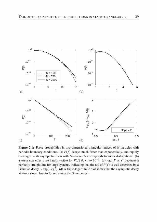
2.3 Triangular lattice

A well-studied geometry for which the force network ensemble yields nontrivial re-sults is that when all particles are of equal size and form a triangular lattice [43,80, 85]. The umbrella sampling allows us to access the statistics beyond f = 5.Fig. 2.1(a) shows that P( f ) decays much faster than exponentially, and that effects ofthe finite size of the system are weak. Figs. 2.1(b,c,d) illustrate that, for increasinglylarge systems, P( f ) rapidly converges to an asymptotic form which is characterizedby a purely Gaussian decay. This can also be seen in Fig. 2.1(c), where we exploitthe fact that we have access to P( f ) over more than 40 decades. Assuming that,for large f , P( f ) ∼ exp(−c f α), one can infer the exponent α from the asymptoticslope of a triple-logarithmic plot in which log10(− log10 P) is plotted as function oflog10 f [20]. Fig. 2.1(d) shows that α = 2.0± 0.1, confirming that the tail of P( f )is well described by a Gaussian decay. Intriguingly, the force distribution is surpris-ingly well approximated at small f by P( f )' 1/3+3 f /4, which hints that a simpleanalytic expression may exist for the triangular lattice. A decent fit over the wholerange of f is given by P( f ) = (a + b f )e−c( f− f0)2

, where a,b are determined by theobserved small- f behavior, and f0,c are determined by 〈 f 〉 = 1 and

∫P( f )d f = 1,

but deviations from the numerical P( f ) can be observed in the tail.

TAIL OF THE CONTACT FORCE DISTRIBUTIONS IN STATIC GRANULAR . . . 39

(a)0 5 10 15

f

10−60

10−40

10−20

100

P(f

)

N = 168N = 780N = 2900

(b)0 2 4 6

f

10−6

10−4

10−2

100

P(f

)

(c)0 100 200

f2

10−60

10−40

10−20

100

P(f

)

(d)−0.5 0.5 1.5

log10 f

−1

0

1

2

log 10

(−

log 10

P(f

))

slope = 2

Figure 2.1: Force probabilities in two-dimensional triangular lattices of N particles withperiodic boundary conditions. (a) P( f ) decays much faster than exponentially, and rapidlyconverges to its asymptotic form with N—larger N corresponds to wider distributions. (b)System size effects are hardly visible for P( f ) down to 10−6. (c) log10 P vs f 2 becomes aperfectly straight line for large systems, indicating that the tail of P( f ) is well described by aGaussian decay ∼ exp(−c f 2). (d) A triple-logarithmic plot shows that the asymptotic decayattains a slope close to 2, confirming the Gaussian tail.

40 CHAPTER 2

2.4 Disordered packings in two dimensions

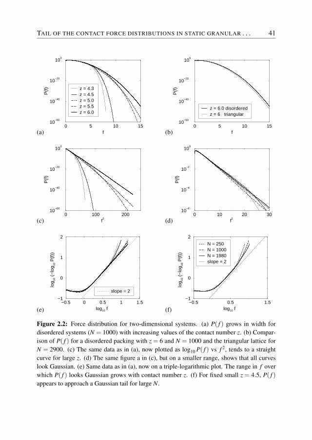
To investigate the effect of packing disorder and coordination number z, we havecreated packings of soft particles with periodic boundary conditions using the com-pression method, see Section 1.4. The coordination number z is controlled by thedegree of compression. Once a packing is obtained, all particle positions are keptfixed, and we subsequently explore the ensemble of force networks for that packing.At this point the interparticle potential is no longer used, so that grain rigidity is nota parameter in the ensemble.

For all 2D disordered packings, P( f ) decays much faster than exponentially, asshown in Fig. 2.2. Comparing the ordered triangular lattices to a disordered sys-tem with equal coordination number, z = 6, we find nearly indistinguishable P( f )(Fig. 2.2(b)). This suggests that the packing (dis)order and preparation history arenot important for P( f ) in the ensemble. However, the contact number influences theasymptotic decay: a lower z leads to a faster decay, although in the restricted rangef < 5, the force distribution appears very close to Gaussian for all z (Fig. 2.2(d)).For the lowest z in particular, this tendency is cut off at large f , which can be clearlyseen in the triple-logarithmic plot (Fig. 2.2(e)), where all curves tend toward a well-defined slope α = 2.0 for intermediate f , but cross over to a much faster decay forlarge f . We suggest that this is a finite-size effect, which is most severe when zapproaches the isostatic point (z = 4), where there are fewer and fewer degrees offreedom available [11, 36, 89]. Indeed, data for z = 4.5 and increasing system sizessuggest that the “kink” in the triple-logarithmic plots becomes less severe for largesystems (Fig. 2.2(f))—our data are not conclusive as to whether this kink will disap-pear for N →∞. In conclusion, for two-dimensional, frictionless systems, the ensem-ble approach yields force distributions P( f ) that decay at least as fast as a Gaussian.

TAIL OF THE CONTACT FORCE DISTRIBUTIONS IN STATIC GRANULAR . . . 41

(a)0 5 10 15

f

10−60

10−40

10−20

100

P(f)

z = 4.3z = 4.5z = 5.0z = 5.5z = 6.0

(b)0 5 10 15

f

10−60

10−40

10−20

100

P(f)

z = 6.0 disorderedz = 6 triangular

(c)0 100 200

f2

10−60

10−40

10−20

100

P(f)

(d)0 10 20 30

f2

10−6

10−4

10−2

100

P(f)

(e)−0.5 0 0.5 1 1.5

log10 f

−1

0

1

2

log 10

(−lo

g 10 P

(f))

slope = 2

(f)−0.5 0.5 1.5

log10 f

−1

0

1

2

log 10

(−lo

g 10 P

(f))

N = 250��N = 1000N = 1980slope = 2

Figure 2.2: Force distribution for two-dimensional systems. (a) P( f ) grows in width fordisordered systems (N = 1000) with increasing values of the contact number z. (b) Compar-ison of P( f ) for a disordered packing with z = 6 and N = 1000 and the triangular lattice forN = 2900. (c) The same data as in (a), now plotted as log10 P( f ) vs f 2, tends to a straightcurve for large z. (d) The same figure a in (c), but on a smaller range, shows that all curveslook Gaussian. (e) Same data as in (a), now on a triple-logarithmic plot. The range in f overwhich P( f ) looks Gaussian grows with contact number z. (f) For fixed small z = 4.5, P( f )appears to approach a Gaussian tail for large N.

42 CHAPTER 2

2.5 Three- and four-dimensional packings

We now turn to three-dimensional systems, which have been generated using molecu-lar dynamics, see section 1.4. Similar to what happens in two dimensions, Fig. 2.3(a)shows that P( f ) decays faster than exponentially, and disordered and regular (fcc)packings have very similar force distributions. However, the decay is now slowerthan Gaussian and much more accurately described by P( f ) ∼ exp(−c f α) with anexponent α = 1.7±0.1 (see Figs. 2.3(c,d)). For comparison we have also included theresult for the triangular lattice, which is seen to decrease significantly more rapidlythan the P( f )’s of the three-dimensional systems. For small systems and small con-tact number (N = 250,z = 9.1), finite-size deviations, similar to those observed intwo dimensions, can be seen. The exponent α has also been determined from thetriple-logarithmic plots of the contact force distributions (Fig. 2.4(a)) for a range ofcontact numbers and system sizes, and in all cases the slope is close to α = 1.7 overa decade.

Surprisingly, we thus find that the dimensionality of the packing determines thenature of the tail of P( f ). Therefore, we have also considered a 4D packing of N =256 with 2681 bonds, leading to z ≈ 20.9. The topology of this network has beenchosen randomly. All bonds vectors were chosen randomly on a 4D unit sphere.Such a packing seems to be a reasonable choice for a typical 4D system, since wehave seen earlier that the behavior of large forces does not strongly depend on thepacking geometry for 2D and 3D systems. In the simulation, we constrain the systemto σαα = 1

4 and σαβ (α 6=β ) = 0. Fig. 2.4(b) shows that for this system α ≈ 1.4.For very large d, the coordination number becomes large as well, reducing cor-

relations between contact forces acting on the same grain. If these correlations com-pletely vanish, then one would expect α = 1 (see also Section 3.4). It would beinteresting to validate if this is really the case for d → ∞.

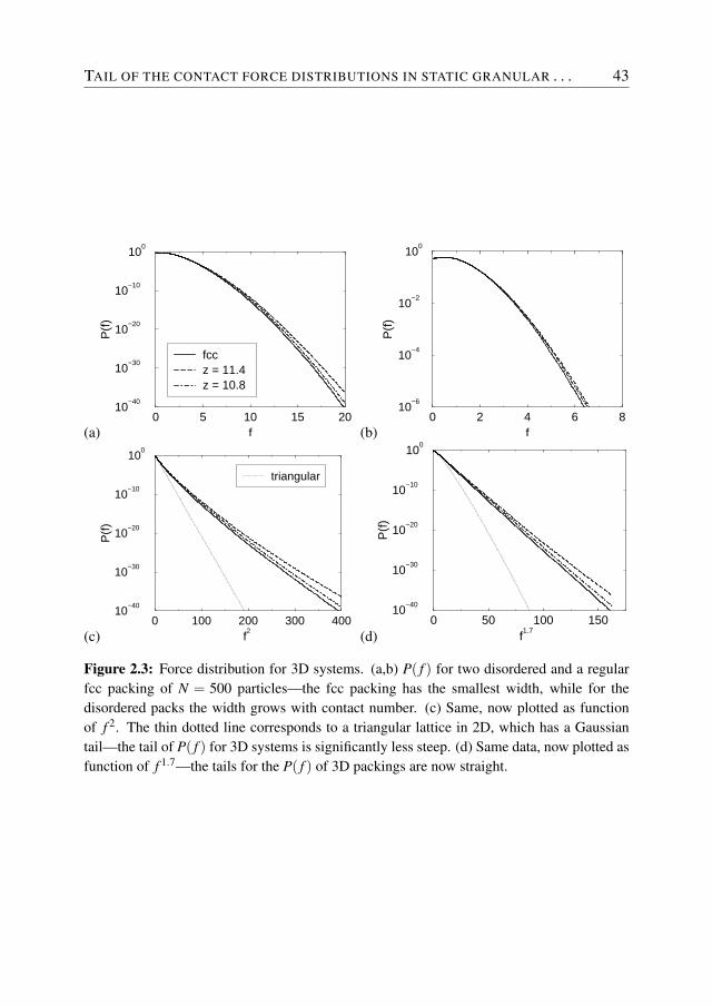
TAIL OF THE CONTACT FORCE DISTRIBUTIONS IN STATIC GRANULAR . . . 43

(a)0 5 10 15 20

f

10−40

10−30

10−20

10−10

100

P(f

)

fccz = 11.4z = 10.8

(b)0 2 4 6 8

f

10−6

10−4

10−2

100

P(f

)

(c)0 100 200 300 400

f2

10−40

10−30

10−20

10−10

100

P(f)

triangular

(d)0 50 100 150

f1.7

10−40

10−30

10−20

10−10

100

P(f)

Figure 2.3: Force distribution for 3D systems. (a,b) P( f ) for two disordered and a regularfcc packing of N = 500 particles—the fcc packing has the smallest width, while for thedisordered packs the width grows with contact number. (c) Same, now plotted as functionof f 2. The thin dotted line corresponds to a triangular lattice in 2D, which has a Gaussiantail—the tail of P( f ) for 3D systems is significantly less steep. (d) Same data, now plotted asfunction of f 1.7—the tails for the P( f ) of 3D packings are now straight.

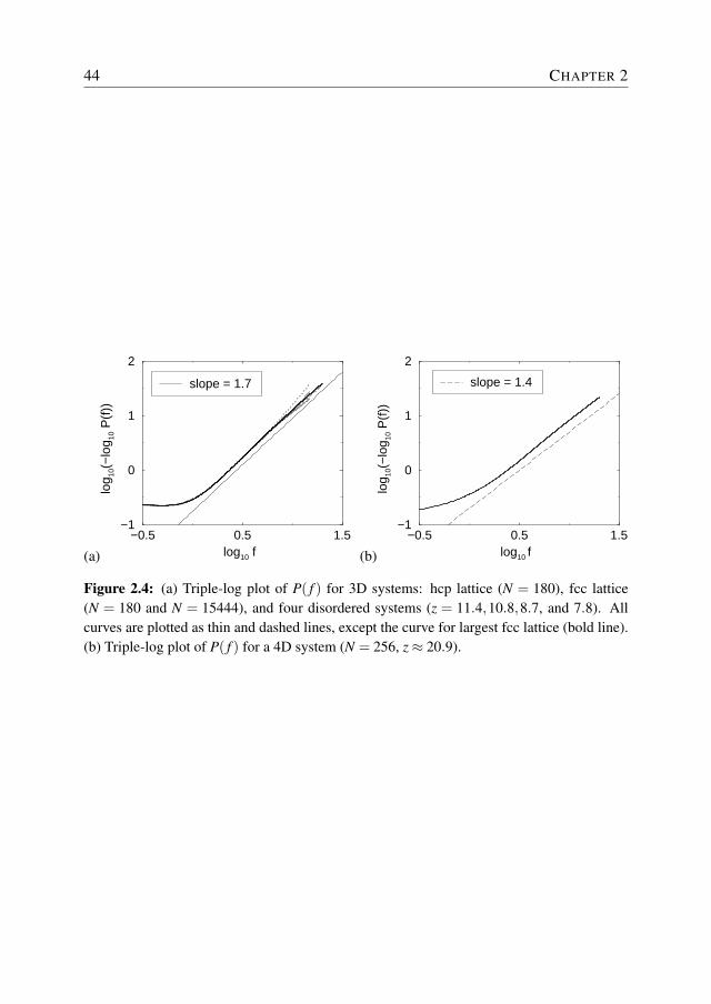
44 CHAPTER 2

(a)−0.5 0.5 1.5

log10 f

−1

0

1

2

log 10

(−lo

g 10 P

(f))

slope = 1.7

(b)−0.5 0.5 1.5

log10 f

−1

0

1

2lo

g 10(−

log 10

P(f)

)slope = 1.4

Figure 2.4: (a) Triple-log plot of P( f ) for 3D systems: hcp lattice (N = 180), fcc lattice(N = 180 and N = 15444), and four disordered systems (z = 11.4,10.8,8.7, and 7.8). Allcurves are plotted as thin and dashed lines, except the curve for largest fcc lattice (bold line).(b) Triple-log plot of P( f ) for a 4D system (N = 256, z≈ 20.9).

TAIL OF THE CONTACT FORCE DISTRIBUTIONS IN STATIC GRANULAR . . . 45

2.6 The effect of shear stress

From experiments on (two-dimensional) sheared packs of photoelastic grains, it wasfound that the distribution broadened significantly, and developed an exponential-like regime in a range up to f = 4〈 f 〉 [25]. The ensemble indeed reproduces thisqualitative feature for packs under shear. As can be seen in Fig. 2.5, however, theredoes not seem to be a simple asymptotic decay. This is because the force anisotropyinduced by the shear stress yields a variation in 〈 f 〉 depending on the orientation ofthe contact [11, 80]. The total P( f ) becomes a superposition over all orientations,of mixed force statistics, and hence lacks a single characteristic feature. The angle-resolved contact force distribution will be discussed in Chapter 4.

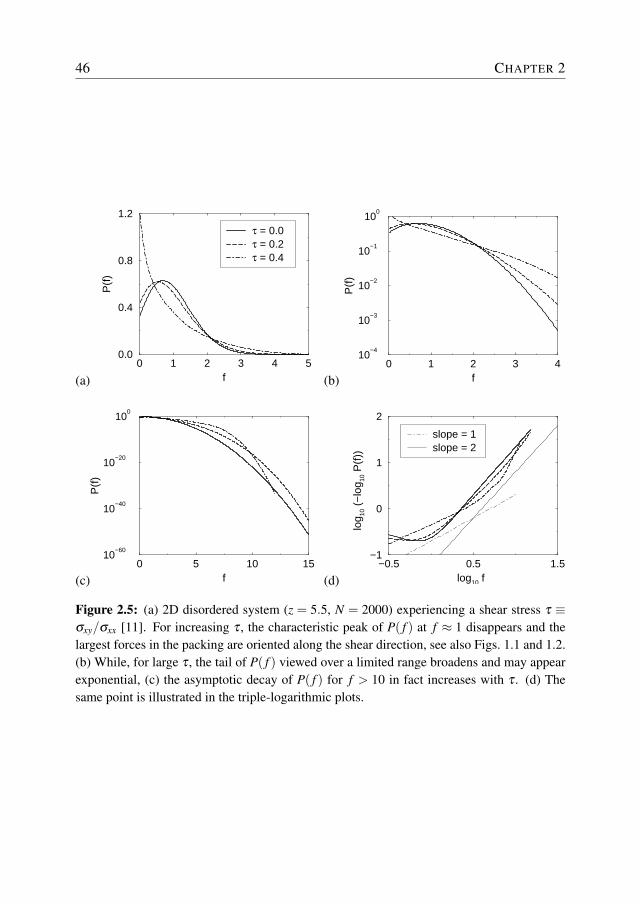
46 CHAPTER 2

(a)0 1 2 3 4 5

f

0.0

0.4

0.8

1.2

P(f)

τ = 0.0τ = 0.2τ = 0.4

(b)0 1 2 3 4

f

10−4

10−3

10−2

10−1

100

P(f

)

(c)0 5 10 15

f

10−60

10−40

10−20

100

P(f

)

(d)−0.5 0.5 1.5

log10 f

−1

0

1

2

log 10

(−

log 10

P(f

))

slope = 1slope = 2

Figure 2.5: (a) 2D disordered system (z = 5.5, N = 2000) experiencing a shear stress τ ≡σxy/σxx [11]. For increasing τ , the characteristic peak of P( f ) at f ≈ 1 disappears and thelargest forces in the packing are oriented along the shear direction, see also Figs. 1.1 and 1.2.(b) While, for large τ , the tail of P( f ) viewed over a limited range broadens and may appearexponential, (c) the asymptotic decay of P( f ) for f > 10 in fact increases with τ . (d) Thesame point is illustrated in the triple-logarithmic plots.

TAIL OF THE CONTACT FORCE DISTRIBUTIONS IN STATIC GRANULAR . . . 47

2.7 Discussion

We have shown for the force network ensemble that the tail of P( f ) decays fasterthan exponentially, in agreement with recent experiments [25, 29], but inconsistentwith others [15, 20–24]. Our results required extremely accurate statistics, beyondthe regime accessible by experiments or conventional simulations. In particular, inexperiments it would be difficult to distinguish an exponent α = 1.7 from 2.0. Never-theless the discrepancy between the exponential data sets [15, 20–24] and the faster-than-exponential data sets [25, 29] cannot be explained away by finite error bars, butis convincing and worthwhile of further investigations.

The experimental and numerical data for P( f ) have been obtained from a widevariety of systems and models, and parameters such as dimensionality, friction, hard-ness of grains vs boundary, and bulk vs boundary measurements may ultimately allplay a role in determining the asymptotics of P( f ). Note that the glass beads usedin the boundary measurements are much harder than the particles used in the bulkmeasurements of [25, 26, 29], and that realistic particle rigidity is difficult to achievein molecular dynamics.

The ensemble can also be extended to include torque balance and to exploreboundary measurements. This will be discussed in Chapters 3 and 4 respectively.A crucial untested assumption in the ensemble is the flat measure, i.e., the samplingof all allowed configurations with equal weight. As argued in Ref. [20], differentexperimental procedures and parameters can lead to a different P( f ), so that the ef-fective sampling of force networks may not be universal.

3

Entropy maximization in the forcenetwork ensemble for granular solids

A long-standing issue in the area of granular media is the tail of the force distribu-tion, in particular whether this is exponential, Gaussian, or even some other form.We demonstrate that conservation of the total area of a reciprocal tiling, a direct con-sequence of local force balance, is crucial for predicting the local stress and forcedistribution. Maximizing entropy while conserving the tiling area and total pressureleads to a distribution of local pressures with a generically Gaussian tail that is in ex-cellent agreement with numerics, both with and without friction and for two differentcontact networks (triangular lattice and square lattice).

This chapter is for a large part based on:B.P. Tighe, A.R.T. van Eerd and T.J.H. VlugtEntropy maximization in the force network ensemble for granular solidsPhys. Rev. Lett. 100, 238001 (2008)

50 CHAPTER 3

3.1 Introduction

There is as yet no clear consensus on the form of the distribution of local stresses ingranular media. Of particular interest is the large-stress tail, which early experimentsfound to be exponential when measured on the boundary [15, 20–24]. More recentmeasurements in the bulk [26, 29], along with numerics [12, 28, 37, 90], find distri-butions that bend downward on a semilogarithmic plot, suggesting faster than expo-nential decay. A number of proposed theories exploit an analogy to the microcanon-ical ensemble to arrive at a Boltzmann-like exponential tail [38, 46, 48, 77, 91–93].These theories should in principle apply to the force network ensemble of Snoeijeret al. [43]. However, in the previous chapter we have unambiguously shown thatthis is not the case: the normal force distributions decay much faster than exponen-tially: P( fn) ∼ exp(−c( fn)α), with α≈2.0 for 2D systems, α≈1.7 for 3D systemsand α≈1.4 for 4D systems (see Chapter 2). As the present statistical mechanics ap-proaches fail to describe simple models like the force network ensemble, they mustbe missing an important ingredient. We argue that local force balance is absolutelycrucial to describe the correct stress statistics. In particular, we show that the pressuredistribution in the force network ensemble directly follows from entropy maximiza-tion, but only when it respects a conserved quantity overlooked in previous theories.This conserved quantity follows from force balance at the grain scale, and leads toexcellent agreement with numerics for both small and large forces.

3.2 Force network ensemble

Snoeijer’s ensemble is composed of all “force networks”, i.e. sets of noncohesivecontact forces on a fixed granular contact network, for which all N grains are in staticforce and torque balance. For packings with more than a critical number of contactsper grain zc, there exist many balanced force networks. The critical coordinationnumber zc equals 4 (3) for frictionless (frictional) 2D packings of disks [43]. All forcenetworks on a contact network with the same global stress tensor and local force andtorque balance can be sampled uniformly by a series of Monte Carlo moves, termed“wheel moves”, see also Section 1.5 and Tighe et al. [80]. As by construction theglobal stress tensor Eq. (1.23) is fixed, the extensive pressure in the system P is

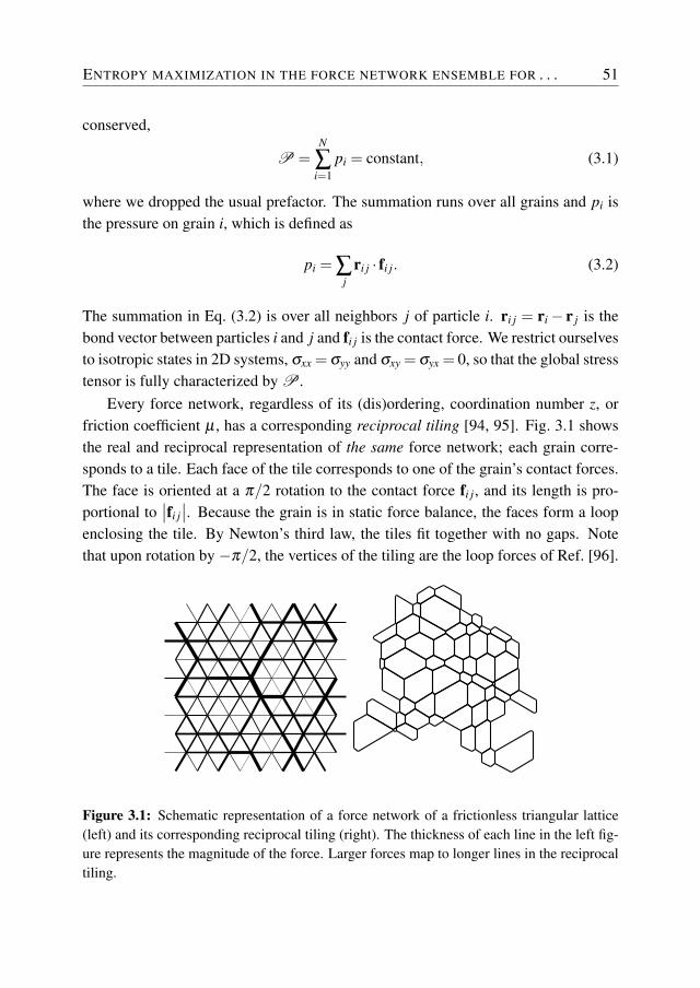
ENTROPY MAXIMIZATION IN THE FORCE NETWORK ENSEMBLE FOR . . . 51

conserved,

P =N

∑i=1

pi = constant, (3.1)

where we dropped the usual prefactor. The summation runs over all grains and pi isthe pressure on grain i, which is defined as

pi = ∑j

ri j · fi j. (3.2)

The summation in Eq. (3.2) is over all neighbors j of particle i. ri j = ri− r j is thebond vector between particles i and j and fi j is the contact force. We restrict ourselvesto isotropic states in 2D systems, σxx = σyy and σxy = σyx = 0, so that the global stresstensor is fully characterized by P .

Every force network, regardless of its (dis)ordering, coordination number z, orfriction coefficient µ , has a corresponding reciprocal tiling [94, 95]. Fig. 3.1 showsthe real and reciprocal representation of the same force network; each grain corre-sponds to a tile. Each face of the tile corresponds to one of the grain’s contact forces.The face is oriented at a π/2 rotation to the contact force fi j, and its length is pro-portional to

∣∣fi j∣∣. Because the grain is in static force balance, the faces form a loop

enclosing the tile. By Newton’s third law, the tiles fit together with no gaps. Notethat upon rotation by −π/2, the vertices of the tiling are the loop forces of Ref. [96].

Figure 3.1: Schematic representation of a force network of a frictionless triangular lattice(left) and its corresponding reciprocal tiling (right). The thickness of each line in the left fig-ure represents the magnitude of the force. Larger forces map to longer lines in the reciprocaltiling.

52 CHAPTER 3

Specifying the boundary forces on a packing establishes the boundaries of itscorresponding tiling, and hence the total area of the tiling. Fixing the global stresstensor in a periodic system has the same effect. Rearrangements of bulk forces,i.e. the wheel moves, correspond to local exchanges of area among tiles. It can beshown that the total tiling area is unaltered by wheel moves, and therefore the areaA is conserved. That is,

A =N

∑i=1

ai = constant. (3.3)

The sum runs over all tiles and ai is the area of tile i:

ai =12

z ·zi−2

∑j=1

zi−1

∑k= j+1

[fi j× fik] . (3.4)

The indices j and k number the zi neighbors of grain i in a right-hand fashion. Theunit vector z = x×y points out of the plane. Area conservation is a global constraintthat results from imposing local force balance. It holds for arbitrary force balancedpackings in 2D with fixed global stress tensor or boundary forces. Area conservationplays a crucial role in determining the statistics of local stresses.

3.3 Entropy maximization

Armed with the insight that the force network ensemble involves two conserved quan-tities, P and A , we explore their implications for the statistics of local stresses.While previous work has incorporated the conservation of P or its equivalent, theconservation of A has heretofore been overlooked. We will show that the conserva-tion of A has a dramatic effect on the force network statistics.

We calculate the probability density P(p) by maximizing entropy while conserv-ing P and A . Each force network corresponds to a set of pressures {pi}, i = 1 . . .N.We define X(p)ω(p)d p as the probability of finding a pressure p in the interval[p, p + ω(p)d p], where ω(p) is the density of states for pressures. The entropy Sis the logarithm of the number of ways of constructing force networks with pressures{pi} consistent with X(p). In the thermodynamic limit [92, 97–99]

S =−∫

∞

0

(X(p) lnX(p)

)ω(p)d p. (3.5)

The experimentally accessible probability density P(p) is related to X(p) by P(p)d p= X(p)ω(p)d p. It is important to note that weighting all force networks equally does

ENTROPY MAXIMIZATION IN THE FORCE NETWORK ENSEMBLE FOR . . . 53

not correspond to a flat measure on the pressures, i.e. ω(p) 6= constant. B.P. Tigheshowed that ω(p) ∝ pν [88]. The value of ν depends on the grain’s coordinationnumber and the friction coefficient. For the frictionless triangular lattice, ν = z− 3.The entropy is maximized subject to Eqs. (3.1) and (3.3), as well as normalization ofP(p). This leads to [88]

〈p〉 = P/N =∫

∞

0pP(p)d p,

〈a〉 = A /N =∫

∞

0〈a(p)〉P(p)d p,

1 =∫

∞

0P(p)d p. (3.6)

〈a(p)〉 =∫

aP(a|p)da is the average area of a tile with perimeter or pressure p;P(a|p) is the conditional probability that a certain tile has area a given its perimeterp. Using the method of Lagrange multipliers, B.P. Tighe et al. [88] have shown thatthe entropy-maximizing density subject to Eqs. (3.6) is

P(p) = Z−1 pν exp [−α p− γ 〈a(p)〉]. (3.7)

Without the constraint on tiling area we would always have γ = 0 and thus an expo-nential tail: Incorporating local force balance by means of the area constraint hasqualitatively changed the form of the distribution. The Lagrange multipliers Z, α ,and γ are determined by substituting Eq. (3.7) in Eqs. (3.6). For frictionless systemsa scaling argument shows that 〈a(p)〉 is quadratic in the thermodynamic limit [88];we write 〈a(p)〉= c〈a〉(p/〈p〉)2 and determine the constant c from numerics. Thusthe probability density P(p) has a generically Gaussian tail, as was already shownnumerically for the normal contact force distribution P( fn). As expected, it will turnout that P(p) and P( fn) have the same asymptotic behavior.

54 CHAPTER 3

3.4 Results

We employ umbrella sampling on a periodic frictionless triangular lattice with N =1840 to numerically determine P(p), see Sections 1.5 and 1.6. To improve samplingof large pressures, we used the maximum pressure on a single grain (pmax(f)) as anorder parameter. A typical snapshot of a force network of this system with a largevalue of pmax is shown in Fig. 3.2. It is important to note that typical force config-urations with a large pmax are fundamentally different from those with a large fmax,see also Fig. 1.8. Typical force configurations with a large pmax have a single grainon which all contact forces are large, while typical force configurations with a largefmax have at least a single grain on which two forces are very large. Therefore, to ac-curately compute P( f ) and P(p) for large forces and pressures respectively separateumbrella sampling simulations are needed.

In all simulations, forces are normalized in such a way that the average normalforce 〈 fn〉 = 1. From the sampled 〈a(p)〉, shown in Fig. 3.3, we extract c ≈ 0.89.Fig. 3.4 contains the corresponding probability density of Eq. (3.7) and its numericalcounterpart. Theory and numerics are in excellent agreement, even for P(p) as lowas 10−8. The slight discrepancies can be attributed to finite size effects and spatialpressure correlations: due to force balance, neighbors of large p grains are morelikely to be at high p themselves. Thus large pressures are less entropically favorablethan suggested by neglecting correlations.

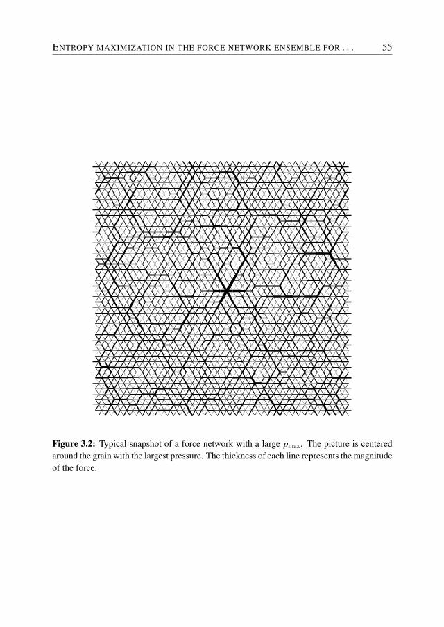
ENTROPY MAXIMIZATION IN THE FORCE NETWORK ENSEMBLE FOR . . . 55

Figure 3.2: Typical snapshot of a force network with a large pmax. The picture is centeredaround the grain with the largest pressure. The thickness of each line represents the magnitudeof the force.

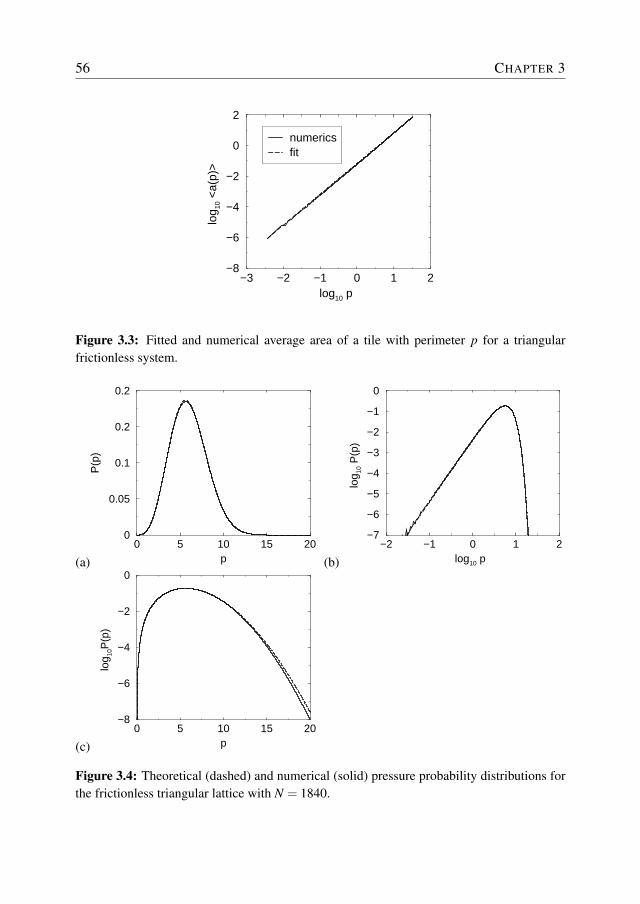
56 CHAPTER 3

−3 −2 −1 0 1 2log10 p

−8

−6

−4

−2

0

2

log 10

<a(

p)>

numericsfit

Figure 3.3: Fitted and numerical average area of a tile with perimeter p for a triangularfrictionless system.

(a)0 5 10 15 20

p

0

0.05

0.1

0.2

0.2

P(p)

(b)−2 −1 0 1 2

log10 p

−7

−6

−5

−4

−3

−2

−1

0

log 10

P(p

)

(c)0 5 10 15 20

p

−8

−6

−4

−2

0

log 10

P(p)

Figure 3.4: Theoretical (dashed) and numerical (solid) pressure probability distributions forthe frictionless triangular lattice with N = 1840.

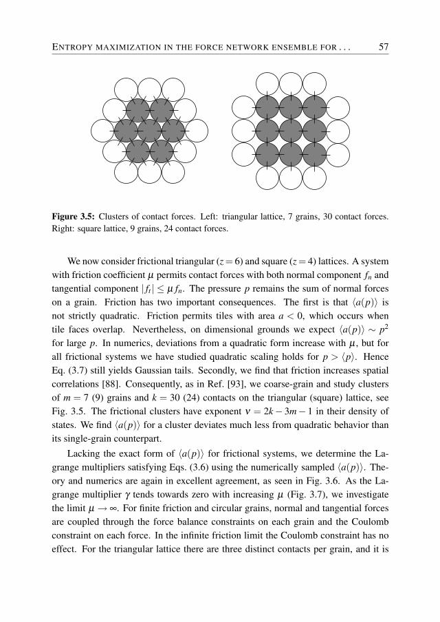
ENTROPY MAXIMIZATION IN THE FORCE NETWORK ENSEMBLE FOR . . . 57

Figure 3.5: Clusters of contact forces. Left: triangular lattice, 7 grains, 30 contact forces.Right: square lattice, 9 grains, 24 contact forces.

We now consider frictional triangular (z = 6) and square (z = 4) lattices. A systemwith friction coefficient µ permits contact forces with both normal component fn andtangential component | ft | ≤ µ fn. The pressure p remains the sum of normal forceson a grain. Friction has two important consequences. The first is that 〈a(p)〉 isnot strictly quadratic. Friction permits tiles with area a < 0, which occurs whentile faces overlap. Nevertheless, on dimensional grounds we expect 〈a(p)〉 ∼ p2

for large p. In numerics, deviations from a quadratic form increase with µ , but forall frictional systems we have studied quadratic scaling holds for p > 〈p〉. HenceEq. (3.7) still yields Gaussian tails. Secondly, we find that friction increases spatialcorrelations [88]. Consequently, as in Ref. [93], we coarse-grain and study clustersof m = 7 (9) grains and k = 30 (24) contacts on the triangular (square) lattice, seeFig. 3.5. The frictional clusters have exponent ν = 2k− 3m− 1 in their density ofstates. We find 〈a(p)〉 for a cluster deviates much less from quadratic behavior thanits single-grain counterpart.

Lacking the exact form of 〈a(p)〉 for frictional systems, we determine the La-grange multipliers satisfying Eqs. (3.6) using the numerically sampled 〈a(p)〉. The-ory and numerics are again in excellent agreement, as seen in Fig. 3.6. As the La-grange multiplier γ tends towards zero with increasing µ (Fig. 3.7), we investigatethe limit µ → ∞. For finite friction and circular grains, normal and tangential forcesare coupled through the force balance constraints on each grain and the Coulombconstraint on each force. In the infinite friction limit the Coulomb constraint has noeffect. For the triangular lattice there are three distinct contacts per grain, and it is

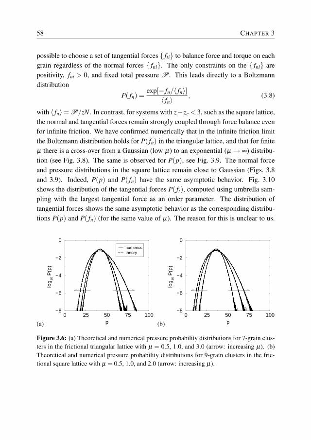
58 CHAPTER 3

possible to choose a set of tangential forces { fti} to balance force and torque on eachgrain regardless of the normal forces { fni}. The only constraints on the { fni} arepositivity, fni > 0, and fixed total pressure P . This leads directly to a Boltzmanndistribution

P( fn) =exp[− fn/〈 fn〉]

〈 fn〉, (3.8)

with 〈 fn〉= P/zN. In contrast, for systems with z−zc < 3, such as the square lattice,the normal and tangential forces remain strongly coupled through force balance evenfor infinite friction. We have confirmed numerically that in the infinite friction limitthe Boltzmann distribution holds for P( fn) in the triangular lattice, and that for finiteµ there is a cross-over from a Gaussian (low µ) to an exponential (µ → ∞) distribu-tion (see Fig. 3.8). The same is observed for P(p), see Fig. 3.9. The normal forceand pressure distributions in the square lattice remain close to Gaussian (Figs. 3.8and 3.9). Indeed, P(p) and P( fn) have the same asymptotic behavior. Fig. 3.10shows the distribution of the tangential forces P( ft), computed using umbrella sam-pling with the largest tangential force as an order parameter. The distribution oftangential forces shows the same asymptotic behavior as the corresponding distribu-tions P(p) and P( fn) (for the same value of µ). The reason for this is unclear to us.

(a)0 25 50 75 100

p

−8

−6

−4

−2

0

log 10

P(p

)

numericstheory

(b)0 25 50 75 100

p

−8

−6

−4

−2

0

log 10

P(p

)

Figure 3.6: (a) Theoretical and numerical pressure probability distributions for 7-grain clus-ters in the frictional triangular lattice with µ = 0.5, 1.0, and 3.0 (arrow: increasing µ). (b)Theoretical and numerical pressure probability distributions for 9-grain clusters in the fric-tional square lattice with µ = 0.5, 1.0, and 2.0 (arrow: increasing µ).

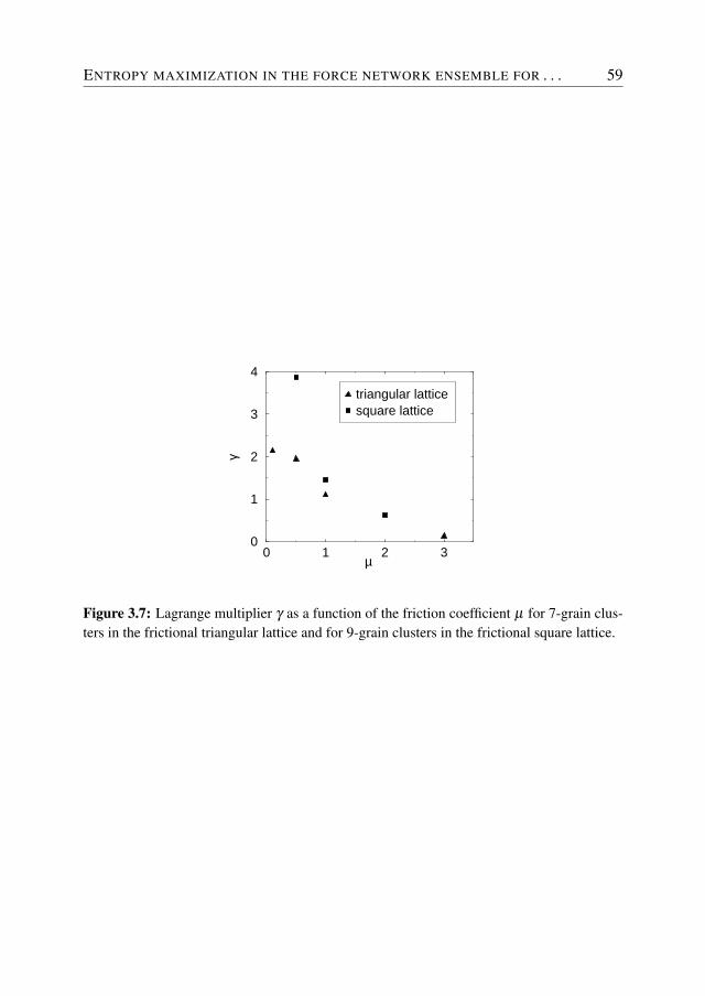
ENTROPY MAXIMIZATION IN THE FORCE NETWORK ENSEMBLE FOR . . . 59

0 1 2 3µ

0

1

2

3

4

γ

triangular latticesquare lattice

Figure 3.7: Lagrange multiplier γ as a function of the friction coefficient µ for 7-grain clus-ters in the frictional triangular lattice and for 9-grain clusters in the frictional square lattice.

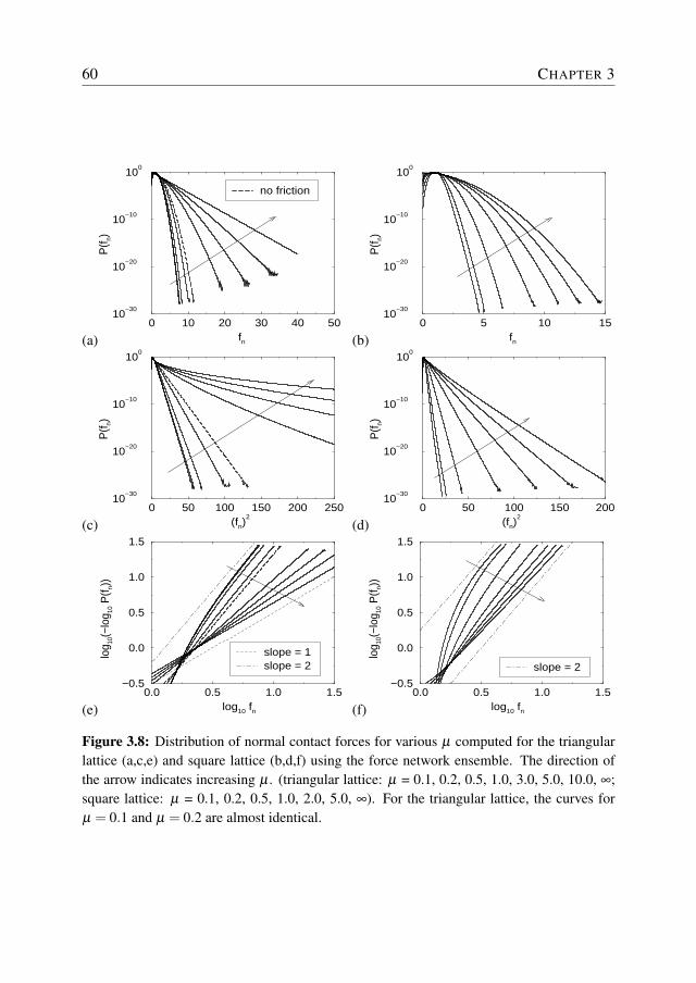
60 CHAPTER 3

(a)0 10 20 30 40 50

fn

10−30

10−20

10−10

100

P(f n)

no friction

(b)0 5 10 15

fn

10−30

10−20

10−10

100

P(f n)

(c)0 50 100 150 200 250

(fn)2

10−30

10−20

10−10

100

P(f n)

(d)0 50 100 150 200

(fn)2

10−30

10−20

10−10

100

P(f n)

(e)0.0 0.5 1.0 1.5

log10 fn

−0.5

0.0

0.5

1.0

1.5

log 10

(−lo

g 10 P

(f n))

slope = 1slope = 2

(f)0.0 0.5 1.0 1.5

log10 fn

−0.5

0.0

0.5

1.0

1.5

log 10

(−lo

g 10 P

(f n))

slope = 2

Figure 3.8: Distribution of normal contact forces for various µ computed for the triangularlattice (a,c,e) and square lattice (b,d,f) using the force network ensemble. The direction ofthe arrow indicates increasing µ . (triangular lattice: µ = 0.1, 0.2, 0.5, 1.0, 3.0, 5.0, 10.0, ∞;square lattice: µ = 0.1, 0.2, 0.5, 1.0, 2.0, 5.0, ∞). For the triangular lattice, the curves forµ = 0.1 and µ = 0.2 are almost identical.

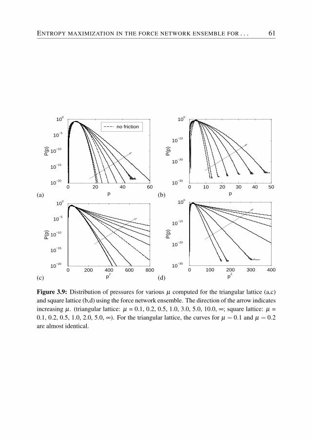
ENTROPY MAXIMIZATION IN THE FORCE NETWORK ENSEMBLE FOR . . . 61

(a)0 20 40 60

p

10−20

10−15

10−10

10−5

100

P(p

)

no friction

(b)0 10 20 30 40 50

p

10−30

10−20

10−10

100

P(p

)

(c)0 200 400 600 800

p2

10−20

10−15

10−10

10−5

100

P(p

)

(d)0 100 200 300 400

p2

10−30

10−20

10−10

100

P(p

)

Figure 3.9: Distribution of pressures for various µ computed for the triangular lattice (a,c)and square lattice (b,d) using the force network ensemble. The direction of the arrow indicatesincreasing µ . (triangular lattice: µ = 0.1, 0.2, 0.5, 1.0, 3.0, 5.0, 10.0, ∞; square lattice: µ =0.1, 0.2, 0.5, 1.0, 2.0, 5.0, ∞). For the triangular lattice, the curves for µ = 0.1 and µ = 0.2are almost identical.

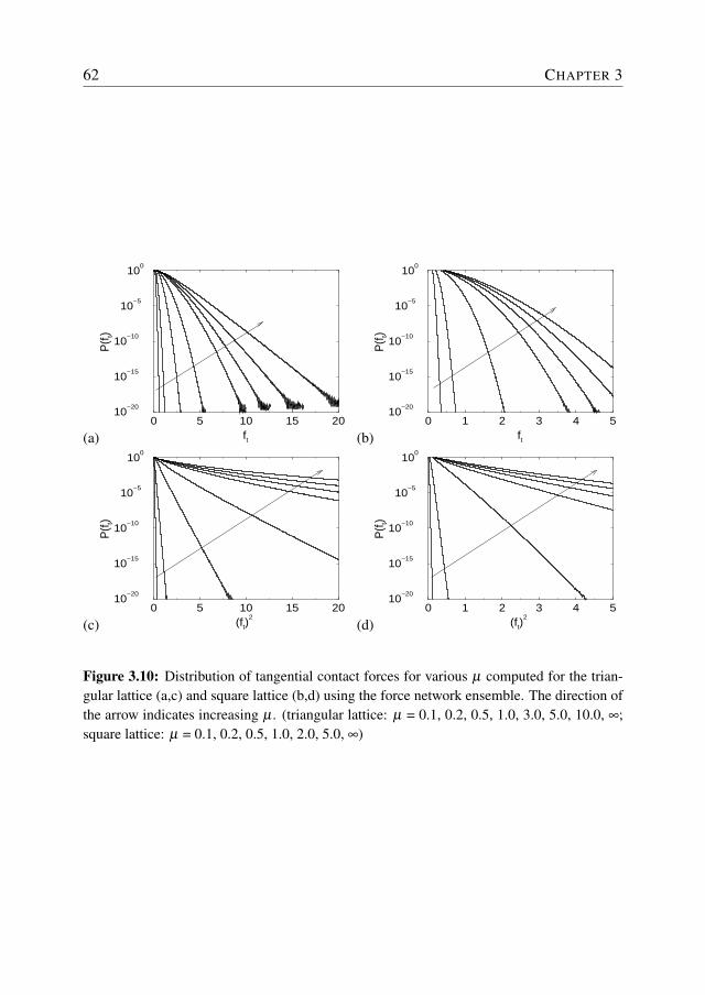
62 CHAPTER 3

(a)0 5 10 15 20

ft

10−20

10−15

10−10

10−5

100

P(f t)

(b)0 1 2 3 4 5

ft

10−20

10−15

10−10

10−5

100

P(f t)

(c)0 5 10 15 20

(ft)2

10−20

10−15

10−10

10−5

100

P(f t)

(d)0 1 2 3 4 5

(ft)2

10−20

10−15

10−10

10−5

100

P(f t)

Figure 3.10: Distribution of tangential contact forces for various µ computed for the trian-gular lattice (a,c) and square lattice (b,d) using the force network ensemble. The direction ofthe arrow indicates increasing µ . (triangular lattice: µ = 0.1, 0.2, 0.5, 1.0, 3.0, 5.0, 10.0, ∞;square lattice: µ = 0.1, 0.2, 0.5, 1.0, 2.0, 5.0, ∞)

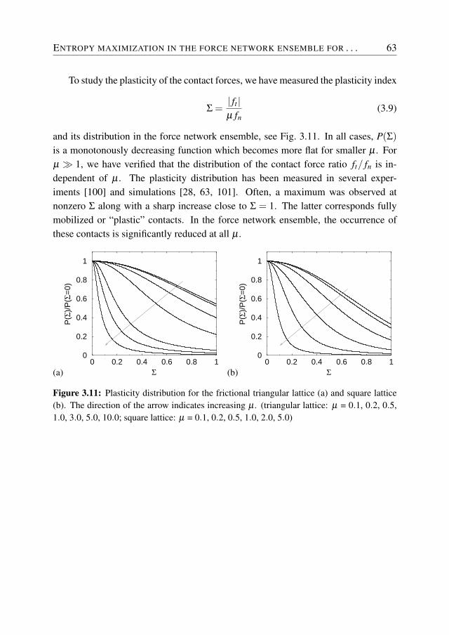
ENTROPY MAXIMIZATION IN THE FORCE NETWORK ENSEMBLE FOR . . . 63

To study the plasticity of the contact forces, we have measured the plasticity index

Σ =| ft |µ fn

(3.9)

and its distribution in the force network ensemble, see Fig. 3.11. In all cases, P(Σ)is a monotonously decreasing function which becomes more flat for smaller µ . Forµ � 1, we have verified that the distribution of the contact force ratio ft/ fn is in-dependent of µ . The plasticity distribution has been measured in several exper-iments [100] and simulations [28, 63, 101]. Often, a maximum was observed atnonzero Σ along with a sharp increase close to Σ = 1. The latter corresponds fullymobilized or “plastic” contacts. In the force network ensemble, the occurrence ofthese contacts is significantly reduced at all µ .

(a)0 0.2 0.4 0.6 0.8 1

Σ

0

0.2

0.4

0.6

0.8

1

P(Σ)

/P(Σ

=0)

(b)0 0.2 0.4 0.6 0.8 1

Σ

0

0.2

0.4

0.6

0.8

1

P(Σ)

/P(Σ

=0)

Figure 3.11: Plasticity distribution for the frictional triangular lattice (a) and square lattice(b). The direction of the arrow indicates increasing µ . (triangular lattice: µ = 0.1, 0.2, 0.5,1.0, 3.0, 5.0, 10.0; square lattice: µ = 0.1, 0.2, 0.5, 1.0, 2.0, 5.0)

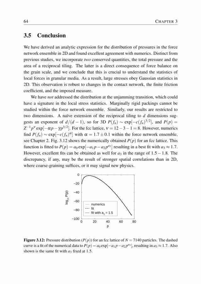
64 CHAPTER 3

3.5 Conclusion

We have derived an analytic expression for the distribution of pressures in the forcenetwork ensemble in 2D and found excellent agreement with numerics. Distinct fromprevious studies, we incorporate two conserved quantities, the total pressure and thearea of a reciprocal tiling. The latter is a direct consequence of force balance onthe grain scale, and we conclude that this is crucial to understand the statistics oflocal forces in granular media. As a result, large stresses obey Gaussian statistics in2D. This observation is robust to changes in the contact network, the finite frictioncoefficient, and the imposed measure.

We have not addressed the distribution at the unjamming transition, which couldhave a signature in the local stress statistics. Marginally rigid packings cannot bestudied within the force network ensemble. Similarly, our results are restricted totwo dimensions. A naïve extension of the reciprocal tiling to d dimensions sug-gests an exponent of d/(d − 1), so for 3D P( fn) ∼ exp[−c( fn)3/2], and P(p) =Z−1 pν exp[−α p−γ p3/2]. For the fcc lattice, ν = 12−3−1 = 8. However, numericsfind P( fn) ∼ exp[−c( fn)α ] with α = 1.7± 0.1 within the force network ensemble,see Chapter 2. Fig. 3.12 shows the numerically obtained P(p) for an fcc lattice. Thisfunction is fitted to P(p) = a0 exp[−a1 p−a2 pa3 ] resulting in a best fit with a3 ≈ 1.7.However, excellent fits can be obtained as well for a3 in the range of 1.5−1.8. Thediscrepancy, if any, may be the result of stronger spatial correlations than in 2D,where coarse-graining suffices, or it may signal new physics.

0 20 40 60 80p

−100

−80

−60

−40

−20

0

log 10

P(p

)

numericsfitfit with a3 = 1.5

Figure 3.12: Pressure distribution (P(p)) for an fcc lattice of N = 7140 particles. The dashedcurve is a fit of the numerical data to P(p) = a0 exp[−a1 p−a2 pa3 ], resulting in a3 ≈ 1.7. Alsoshown is the same fit with a3 fixed at 1.5.

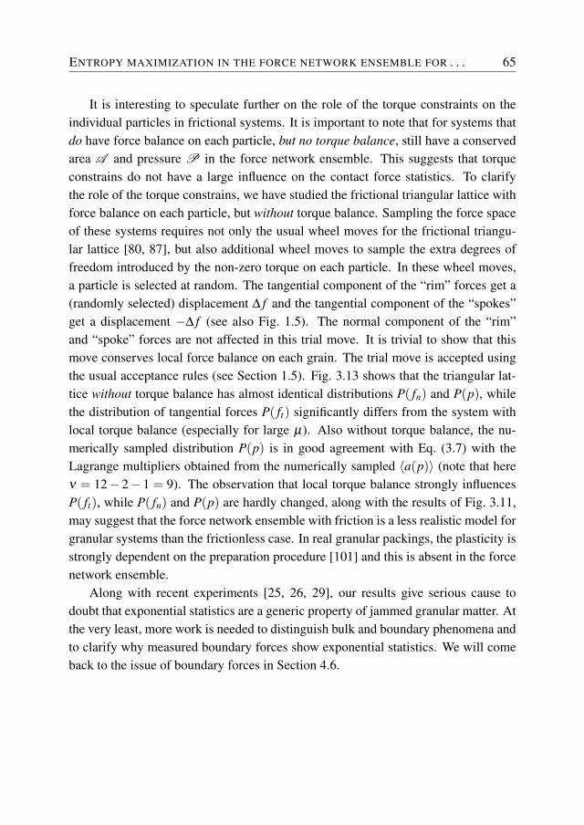
ENTROPY MAXIMIZATION IN THE FORCE NETWORK ENSEMBLE FOR . . . 65

It is interesting to speculate further on the role of the torque constraints on theindividual particles in frictional systems. It is important to note that for systems thatdo have force balance on each particle, but no torque balance, still have a conservedarea A and pressure P in the force network ensemble. This suggests that torqueconstrains do not have a large influence on the contact force statistics. To clarifythe role of the torque constrains, we have studied the frictional triangular lattice withforce balance on each particle, but without torque balance. Sampling the force spaceof these systems requires not only the usual wheel moves for the frictional triangu-lar lattice [80, 87], but also additional wheel moves to sample the extra degrees offreedom introduced by the non-zero torque on each particle. In these wheel moves,a particle is selected at random. The tangential component of the “rim” forces get a(randomly selected) displacement ∆ f and the tangential component of the “spokes”get a displacement −∆ f (see also Fig. 1.5). The normal component of the “rim”and “spoke” forces are not affected in this trial move. It is trivial to show that thismove conserves local force balance on each grain. The trial move is accepted usingthe usual acceptance rules (see Section 1.5). Fig. 3.13 shows that the triangular lat-tice without torque balance has almost identical distributions P( fn) and P(p), whilethe distribution of tangential forces P( ft) significantly differs from the system withlocal torque balance (especially for large µ). Also without torque balance, the nu-merically sampled distribution P(p) is in good agreement with Eq. (3.7) with theLagrange multipliers obtained from the numerically sampled 〈a(p)〉 (note that hereν = 12− 2− 1 = 9). The observation that local torque balance strongly influencesP( ft), while P( fn) and P(p) are hardly changed, along with the results of Fig. 3.11,may suggest that the force network ensemble with friction is a less realistic model forgranular systems than the frictionless case. In real granular packings, the plasticity isstrongly dependent on the preparation procedure [101] and this is absent in the forcenetwork ensemble.

Along with recent experiments [25, 26, 29], our results give serious cause todoubt that exponential statistics are a generic property of jammed granular matter. Atthe very least, more work is needed to distinguish bulk and boundary phenomena andto clarify why measured boundary forces show exponential statistics. We will comeback to the issue of boundary forces in Section 4.6.

66 CHAPTER 3

(a)0 5 10 15 20 25

fn

10−25

10−20

10−15

10−10

10−5

100

P(f n)

(b)0 10 20 30 40

p

10−20

10−15

10−10

10−5

100

P(p)

(c)0 1 2 3 4 5

ft

10−8

10−6

10−4

10−2

100

102

P(f t)

Figure 3.13: Distribution of normal contact forces (a), pressures (b) and tangential forces (c)computed for the triangular lattice of frictional particles using the force network ensemble.The solid lines show the distributions without torque balance and the dashed lines show thedistributions with torque balance. The direction of the arrow indicates increasing µ (0.1, 1.0,5.0).

4

Extended numerical study of the forcenetwork ensemble

68 CHAPTER 4

4.1 Introduction

In this chapter we will use numerical simulations to study several aspects of the forcenetwork ensemble in more detail. In particular, we focus on the details of the stressconstraints and finite-size effects for the frictionless triangular lattice (Section 4.2),the angle resolved contact force distribution (Section 4.3), finite-size effects and themaximum possible force of a certain network of contact forces (Section 4.4), thedimensionality of the space spanned by all solutions (Section 4.5) and the effect ofboundaries (Section 4.6). In the last part of this chapter (Section 4.7), we will investi-gate a crucial and longstanding question: how well does the force network ensembledescribe systems with “real” interactions?

4.2 Details of the stress constraints and finite-size effects

In Section 1.5 we introduced a force scale by imposing 〈 f 〉 = 1. In case that |ri j| =1, this directly results in σxx + σyy (+σzz) = 1. For d dimensional systems underisotropic pressure, it is therefore convenient to choose a force scale such that σxx =σyy (= σzz) = 1/d. However, in Ref. [102] the rather unphysical constraint σxx +σyy = 1 was used instead. With the latter constraint, small anisotropic pressure fluc-tuations occur.

Monte Carlo simulations in the force network ensemble are used to study thecontact force distribution for the triangular lattice for both isotropic and anisotropicpressure. We also unravel the effect of the system size N for both constraints. Theresults are shown in Fig. 4.1. Contact force distributions calculated with σxx = σyy =12 show no differences at forces below f = 5, but a finite size effect is observed forlarger forces, converging to a Gaussian distribution (see also Section 2.3). Contactforce distributions calculated with the anisotropic constraint σxx + σyy = 1 convergeto the same Gaussian distribution, but the finite size effect is much larger. The reasonfor this is that for small systems, the fluctuations of σxx and σyy around 1

2 are quitelarge. For larger systems, these fluctuations become smaller so eventually σxx ≈ 1

2and σyy ≈ 1

2 . From now on, for regular packings we use the constraint σxx = σyy(=σzz) = 1

d , because it is the most physical one.

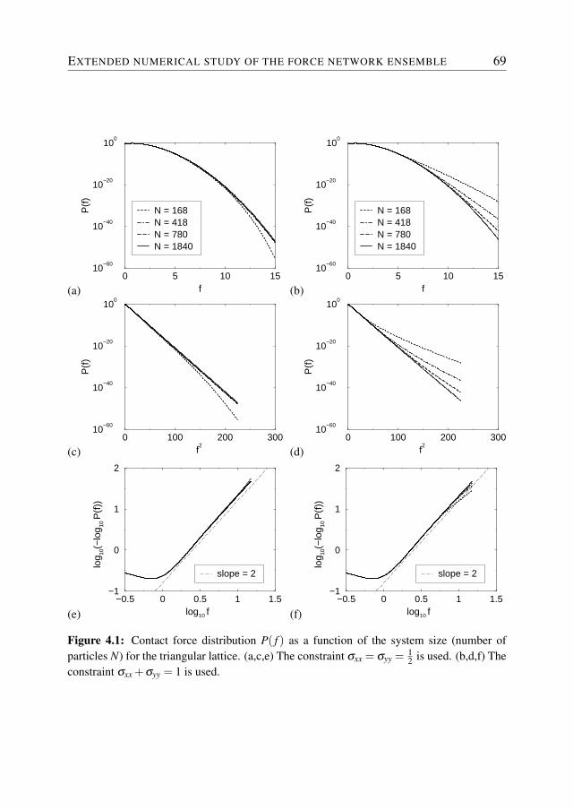
EXTENDED NUMERICAL STUDY OF THE FORCE NETWORK ENSEMBLE 69

(a)0 5 10 15

f

10−60

10−40

10−20

100

P(f)

N = 168N = 418N = 780N = 1840

(b)0 5 10 15

f

10−60

10−40

10−20

100

P(f)

N = 168N = 418N = 780N = 1840

(c)0 100 200 300

f2

10−60

10−40

10−20

100

P(f)

(d)0 100 200 300

f2

10−60

10−40

10−20

100P(

f)

(e)−0.5 0 0.5 1 1.5

log10 f

−1

0

1

2

log 10

(−lo

g 10 P

(f))

slope = 2

(f)−0.5 0 0.5 1 1.5

log10 f

−1

0

1

2

log 10

(−lo

g 10 P

(f))

slope = 2

Figure 4.1: Contact force distribution P( f ) as a function of the system size (number ofparticles N) for the triangular lattice. (a,c,e) The constraint σxx = σyy = 1

2 is used. (b,d,f) Theconstraint σxx +σyy = 1 is used.

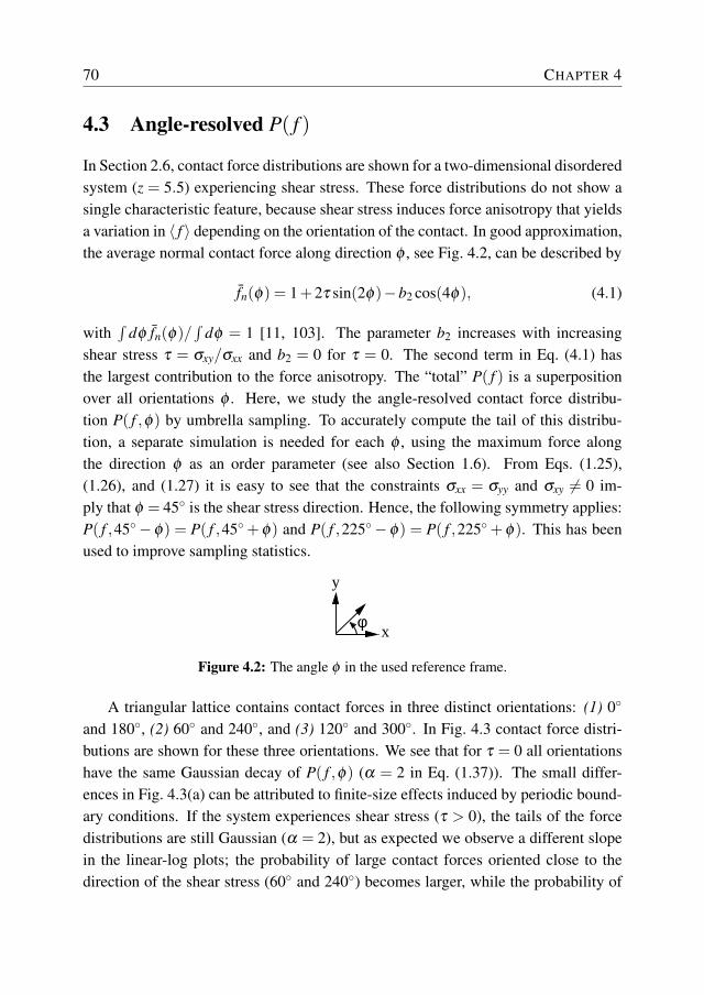
70 CHAPTER 4

4.3 Angle-resolved P( f )

In Section 2.6, contact force distributions are shown for a two-dimensional disorderedsystem (z = 5.5) experiencing shear stress. These force distributions do not show asingle characteristic feature, because shear stress induces force anisotropy that yieldsa variation in 〈 f 〉 depending on the orientation of the contact. In good approximation,the average normal contact force along direction φ , see Fig. 4.2, can be described by

fn(φ) = 1+2τ sin(2φ)−b2 cos(4φ), (4.1)

with∫

dφ fn(φ)/∫

dφ = 1 [11, 103]. The parameter b2 increases with increasingshear stress τ = σxy/σxx and b2 = 0 for τ = 0. The second term in Eq. (4.1) hasthe largest contribution to the force anisotropy. The “total” P( f ) is a superpositionover all orientations φ . Here, we study the angle-resolved contact force distribu-tion P( f ,φ) by umbrella sampling. To accurately compute the tail of this distribu-tion, a separate simulation is needed for each φ , using the maximum force alongthe direction φ as an order parameter (see also Section 1.6). From Eqs. (1.25),(1.26), and (1.27) it is easy to see that the constraints σxx = σyy and σxy 6= 0 im-ply that φ = 45◦ is the shear stress direction. Hence, the following symmetry applies:P( f ,45◦−φ) = P( f ,45◦ + φ) and P( f ,225◦−φ) = P( f ,225◦ + φ). This has beenused to improve sampling statistics.

x

y

φ

Figure 4.2: The angle φ in the used reference frame.

A triangular lattice contains contact forces in three distinct orientations: (1) 0◦

and 180◦, (2) 60◦ and 240◦, and (3) 120◦ and 300◦. In Fig. 4.3 contact force distri-butions are shown for these three orientations. We see that for τ = 0 all orientationshave the same Gaussian decay of P( f ,φ) (α = 2 in Eq. (1.37)). The small differ-ences in Fig. 4.3(a) can be attributed to finite-size effects induced by periodic bound-ary conditions. If the system experiences shear stress (τ > 0), the tails of the forcedistributions are still Gaussian (α = 2), but as expected we observe a different slopein the linear-log plots; the probability of large contact forces oriented close to thedirection of the shear stress (60◦ and 240◦) becomes larger, while the probability of

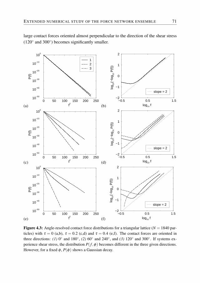
EXTENDED NUMERICAL STUDY OF THE FORCE NETWORK ENSEMBLE 71

large contact forces oriented almost perpendicular to the direction of the shear stress(120◦ and 300◦) becomes significantly smaller.

(a)0 50 100 150 200 250

f2

10−50

10−40

10−30

10−20

10−10

100

P(f

)

123

(b)−0.5 0.5 1.5

log10 f

−2

−1

0

1

2

log 10

(−lo

g 10 P

(f))

slope = 2

(c)0 50 100 150 200 250

f2

10−50

10−40

10−30

10−20

10−10

100

P(f

)

(d)−0.5 0.5 1.5

log10 f

−2

−1

0

1

2lo

g 10(−

log 10

P(f)

)

slope = 2

(e)0 50 100 150 200 250

f2

10−50

10−40

10−30

10−20

10−10

100

P(f

)

(f)−0.5 0.5 1.5

log10 f

−2

−1

0

1

2

log 10

(−lo

g 10 P

(f))

slope = 2

Figure 4.3: Angle-resolved contact force distributions for a triangular lattice (N = 1840 par-ticles) with τ = 0 (a,b), τ = 0.2 (c,d) and τ = 0.4 (e,f). The contact forces are oriented inthree directions: (1) 0◦ and 180◦, (2) 60◦ and 240◦, and (3) 120◦ and 300◦. If systems ex-perience shear stress, the distribution P( f ,φ) becomes different in the three given directions.However, for a fixed φ , P(φ) shows a Gaussian decay.

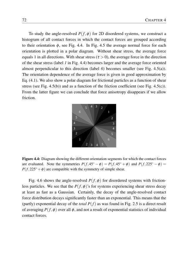
72 CHAPTER 4

To study the angle-resolved P( f ,φ) for 2D disordered systems, we construct ahistogram of all contact forces in which the contact forces are grouped accordingto their orientation φ , see Fig. 4.4. In Fig. 4.5 the average normal force for eachorientation is plotted in a polar diagram. Without shear stress, the average forceequals 1 in all directions. With shear stress (τ > 0), the average force in the directionof the shear stress (label 1 in Fig. 4.4) becomes larger and the average force orientedalmost perpendicular to this direction (label 6) becomes smaller (see Fig. 4.5(a)).The orientation dependence of the average force is given in good approximation byEq. (4.1). We also show a polar diagram for frictional particles as a function of shearstress (see Fig. 4.5(b)) and as a function of the friction coefficient (see Fig. 4.5(c)).From the latter figure we can conclude that force anisotropy disappears if we allowfriction.

1

2

5

5

43

1

3 24

6

2

34

3 4

5

6

52

Figure 4.4: Diagram showing the different orientation segments for which the contact forcesare evaluated. Note the symmetries P( f ,45◦ − φ) = P( f ,45◦ + φ) and P( f ,225◦ − φ) =P( f ,225◦+φ) are compatible with the symmetry of simple shear.

Fig. 4.6 shows the angle-resolved P( f ,φ) for disordered systems with friction-less particles. We see that the P( f ,φ)’s for systems experiencing shear stress decayat least as fast as a Gaussian. Certainly, the decay of the angle-resolved contactforce distribution decays significantly faster than an exponential. This means that the(partly) exponential decay of the total P( f ) as was found in Fig. 2.5 is a direct resultof averaging P( f ,φ) over all φ , and not a result of exponential statistics of individualcontact forces.

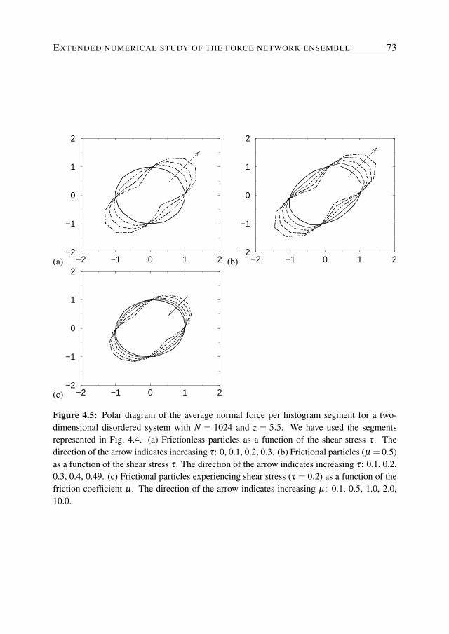
EXTENDED NUMERICAL STUDY OF THE FORCE NETWORK ENSEMBLE 73

(a) −2 −1 0 1 2−2

−1

0

1

2

(b) −2 −1 0 1 2−2

−1

0

1

2

(c) −2 −1 0 1 2−2

−1

0

1

2

Figure 4.5: Polar diagram of the average normal force per histogram segment for a two-dimensional disordered system with N = 1024 and z = 5.5. We have used the segmentsrepresented in Fig. 4.4. (a) Frictionless particles as a function of the shear stress τ . Thedirection of the arrow indicates increasing τ: 0, 0.1, 0.2, 0.3. (b) Frictional particles (µ = 0.5)as a function of the shear stress τ . The direction of the arrow indicates increasing τ: 0.1, 0.2,0.3, 0.4, 0.49. (c) Frictional particles experiencing shear stress (τ = 0.2) as a function of thefriction coefficient µ . The direction of the arrow indicates increasing µ: 0.1, 0.5, 1.0, 2.0,10.0.

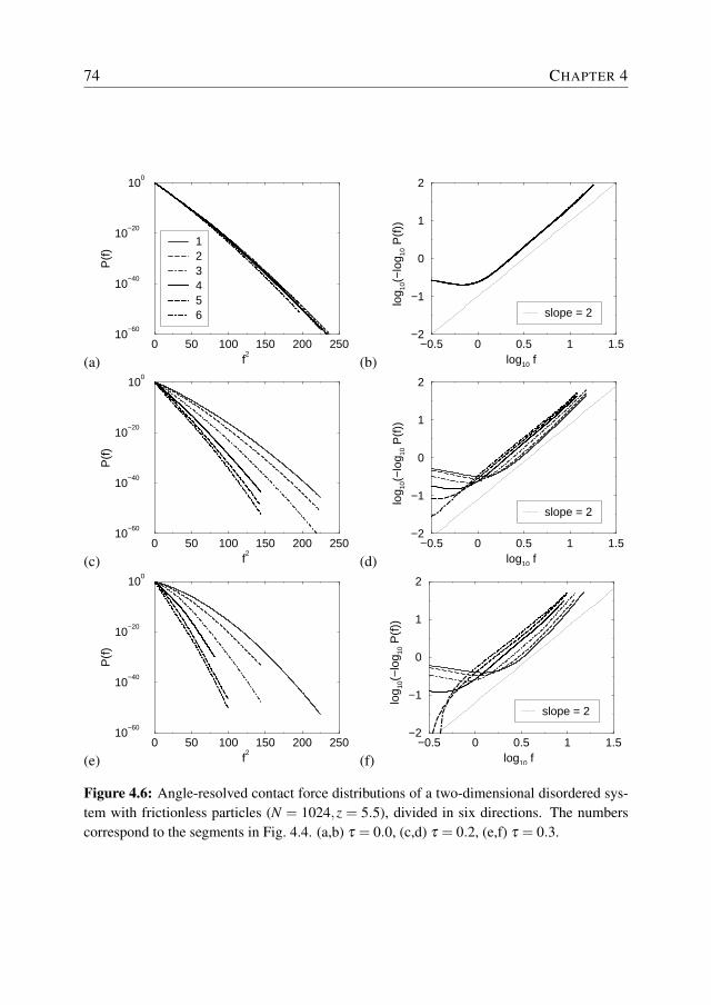
74 CHAPTER 4

(a)0 50 100 150 200 250

f2

10−60

10−40

10−20

100

P(f

)

123456

(b)−0.5 0 0.5 1 1.5

log10 f

−2

−1

0

1

2

log 10

(−lo

g 10 P

(f))

slope = 2

(c)0 50 100 150 200 250

f2

10−60

10−40

10−20

100

P(f

)

(d)−0.5 0 0.5 1 1.5

log10 f

−2

−1

0

1

2lo

g 10(−

log 10

P(f

))

slope = 2

(e)0 50 100 150 200 250

f2

10−60

10−40

10−20

100

P(f

)

(f)−0.5 0 0.5 1 1.5

log10 f

−2

−1

0

1

2

log 10

(−lo

g 10 P

(f))

slope = 2

Figure 4.6: Angle-resolved contact force distributions of a two-dimensional disordered sys-tem with frictionless particles (N = 1024,z = 5.5), divided in six directions. The numberscorrespond to the segments in Fig. 4.4. (a,b) τ = 0.0, (c,d) τ = 0.2, (e,f) τ = 0.3.

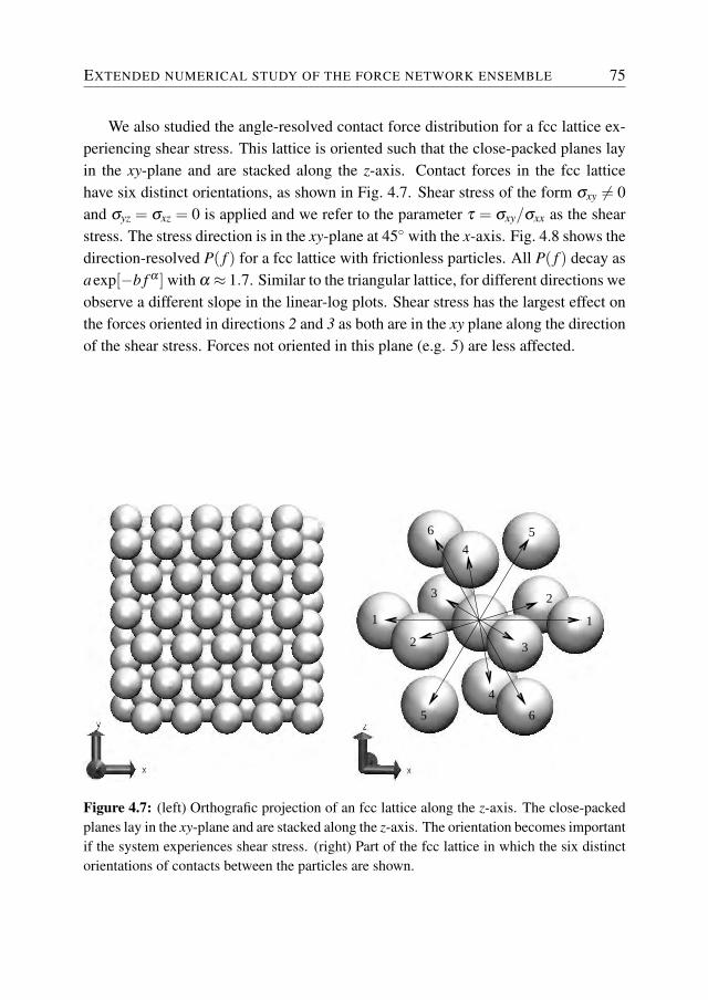
EXTENDED NUMERICAL STUDY OF THE FORCE NETWORK ENSEMBLE 75

We also studied the angle-resolved contact force distribution for a fcc lattice ex-periencing shear stress. This lattice is oriented such that the close-packed planes layin the xy-plane and are stacked along the z-axis. Contact forces in the fcc latticehave six distinct orientations, as shown in Fig. 4.7. Shear stress of the form σxy 6= 0and σyz = σxz = 0 is applied and we refer to the parameter τ = σxy/σxx as the shearstress. The stress direction is in the xy-plane at 45◦ with the x-axis. Fig. 4.8 shows thedirection-resolved P( f ) for a fcc lattice with frictionless particles. All P( f ) decay asaexp[−b f α ] with α ≈ 1.7. Similar to the triangular lattice, for different directions weobserve a different slope in the linear-log plots. Shear stress has the largest effect onthe forces oriented in directions 2 and 3 as both are in the xy plane along the directionof the shear stress. Forces not oriented in this plane (e.g. 5) are less affected.

3

2

211

5 64

64

5

3

Figure 4.7: (left) Orthografic projection of an fcc lattice along the z-axis. The close-packedplanes lay in the xy-plane and are stacked along the z-axis. The orientation becomes importantif the system experiences shear stress. (right) Part of the fcc lattice in which the six distinctorientations of contacts between the particles are shown.

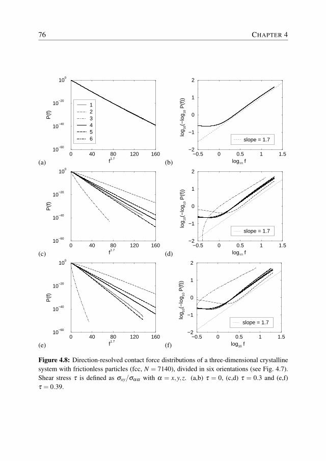
76 CHAPTER 4

(a)0 40 80 120 160

f1.7

10−60

10−40

10−20

100

P(f

)

123456

(b)−0.5 0 0.5 1 1.5

log10 f

−2

−1

0

1

2

log 10

(−lo

g 10 P

(f))

slope = 1.7

(c)0 40 80 120 160

f1.7

10−60

10−40

10−20

100

P(f

)

(d)−0.5 0 0.5 1 1.5

log10 f

−2

−1

0

1

2

log 10

(−lo

g 10 P

(f))

slope = 1.7

(e)0 40 80 120 160

f1.7

10−60

10−40

10−20

100

P(f

)

(f)−0.5 0 0.5 1 1.5

log10 f

−2

−1

0

1

2

log 10

(−lo

g 10 P

(f))

slope = 1.7

Figure 4.8: Direction-resolved contact force distributions of a three-dimensional crystallinesystem with frictionless particles (fcc, N = 7140), divided in six orientations (see Fig. 4.7).Shear stress τ is defined as σxy/σαα with α = x,y,z. (a,b) τ = 0, (c,d) τ = 0.3 and (e,f)τ = 0.39.

EXTENDED NUMERICAL STUDY OF THE FORCE NETWORK ENSEMBLE 77

4.4 Maximum possible force inside a packing

In Section 2.4 we have seen that for disordered packings in 2D, finite-size effectsoccur for the contact force distribution P( f ), especially for low coordination numbers(z). One would observe such finite-size effects for forces close to the maximum forcethat a certain packing can sustain. When the maximum force of a packing ( fmax(f))is close to the maximum force that a certain packing can sustain, P( f ) will show avery sharp decrease. Eventually, P( f ) will decrease to zero for any packing [85].

In principle, conventional umbrella sampling [52] can be used to determine themaximum possible fmax. However, a huge number of iterations will be necessary asP( f ) will become extremely small close to the maximum possible fmax. To efficientlycompute the maximum possible fmax for a given packing, we use the central idea ofthe recently proposed random-walk algorithm of Wang and Landau [104, 105]. In thisscheme, a random walk is performed in the space of all possible force networks f. Thesimulation is started by setting a certain function κ( fmax) = 1 for all fmax. Startingfrom a particular solution f = f0, we perform a Monte Carlo scheme to sample allpossible force networks (see section 1.5). Trial moves that result in a configurationfor which all fn,i ≥ 0 are accepted with a probability

Pacc(o→ n) = min(

1,κ( fmax(o))κ( fmax(n))

). (4.2)

in which o and n are used to denote the old and new configuration respectively. Thecrucial difference with conventional Monte Carlo is that each time a force networkwith a certain fmax is visited, κ( fmax) is updated as follows: κ( fmax)→ κ( fmax)×min which m > 1 (typically m = 2). This means that this scheme does not obey de-tailed balance. After many trial moves, eventually all possible values of fmax willbe visited with (approximately) equal probability. From this, the maximum possibleforce of a certain contact network can be estimated. In the original version algo-rithm [104, 105], the parameter m is slowly decreased from 2 to 1+δ in a controlledway (typically δ ≈ 10−9), such that eventually configurations are sampled with aprobability inversely proportional to the density of states. In our case, we are onlyinterested in the maximum possible force that a packing can sustain and therefore wecan safely set m = 2.

Fig. 4.9(a) shows the computed maximum possible force in 2D disordered sys-tems. Indeed, the maximum possible force increases with N and strongly dependson the coordination number z. In Fig. 4.9(b), the corresponding P( f ) along with the

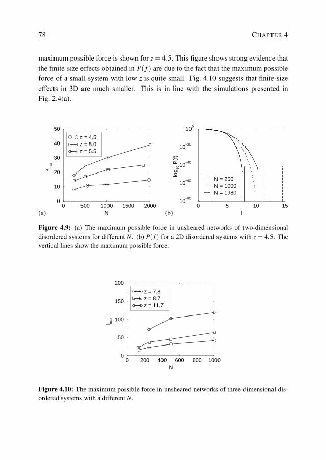
78 CHAPTER 4

maximum possible force is shown for z = 4.5. This figure shows strong evidence thatthe finite-size effects obtained in P( f ) are due to the fact that the maximum possibleforce of a small system with low z is quite small. Fig. 4.10 suggests that finite-sizeeffects in 3D are much smaller. This is in line with the simulations presented inFig. 2.4(a).

(a)0 500 1000 1500 2000

N

0

10

20

30

40

50

f max

z = 4.5z = 5.0z = 5.5

(b)0 5 10 15

f

10−80

10−60

10−40

10−20

100

log 10

P(f)

N = 250N = 1000N = 1980

Figure 4.9: (a) The maximum possible force in unsheared networks of two-dimensionaldisordered systems for different N. (b) P( f ) for a 2D disordered systems with z = 4.5. Thevertical lines show the maximum possible force.

0 200 400 600 800 1000N

0

50

100

150

200

f max

z = 7.8z = 8.7z = 11.7

Figure 4.10: The maximum possible force in unsheared networks of three-dimensional dis-ordered systems with a different N.

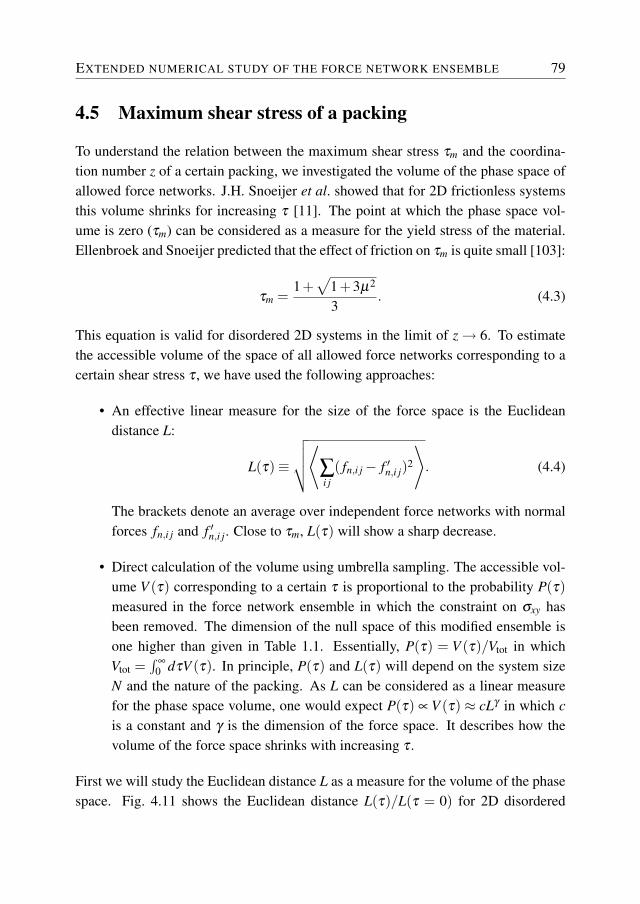
EXTENDED NUMERICAL STUDY OF THE FORCE NETWORK ENSEMBLE 79

4.5 Maximum shear stress of a packing

To understand the relation between the maximum shear stress τm and the coordina-tion number z of a certain packing, we investigated the volume of the phase space ofallowed force networks. J.H. Snoeijer et al. showed that for 2D frictionless systemsthis volume shrinks for increasing τ [11]. The point at which the phase space vol-ume is zero (τm) can be considered as a measure for the yield stress of the material.Ellenbroek and Snoeijer predicted that the effect of friction on τm is quite small [103]:

τm =1+√

1+3µ2

3. (4.3)

This equation is valid for disordered 2D systems in the limit of z → 6. To estimatethe accessible volume of the space of all allowed force networks corresponding to acertain shear stress τ , we have used the following approaches:

• An effective linear measure for the size of the force space is the Euclideandistance L:

L(τ)≡

√√√√⟨∑i j

( fn,i j− f ′n,i j)2

⟩. (4.4)

The brackets denote an average over independent force networks with normalforces fn,i j and f ′n,i j. Close to τm, L(τ) will show a sharp decrease.

• Direct calculation of the volume using umbrella sampling. The accessible vol-ume V (τ) corresponding to a certain τ is proportional to the probability P(τ)measured in the force network ensemble in which the constraint on σxy hasbeen removed. The dimension of the null space of this modified ensemble isone higher than given in Table 1.1. Essentially, P(τ) = V (τ)/Vtot in whichVtot =

∫∞

0 dτV (τ). In principle, P(τ) and L(τ) will depend on the system sizeN and the nature of the packing. As L can be considered as a linear measurefor the phase space volume, one would expect P(τ) ∝ V (τ) ≈ cLγ in which cis a constant and γ is the dimension of the force space. It describes how thevolume of the force space shrinks with increasing τ .

First we will study the Euclidean distance L as a measure for the volume of the phasespace. Fig. 4.11 shows the Euclidean distance L(τ)/L(τ = 0) for 2D disordered

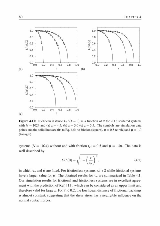
80 CHAPTER 4

(a)0.0 0.2 0.4 0.6 0.8 1.0

τ

0.0

0.2

0.4

0.6

0.8

1.0

L(τ)

/L(0

)

(b)0.0 0.2 0.4 0.6 0.8 1.0

τ

0.0

0.2

0.4

0.6

0.8

1.0

L(τ)

/L(0

)

(c)0.0 0.2 0.4 0.6 0.8 1.0

τ

0.0

0.2

0.4

0.6

0.8

1.0

L(τ)

/L(0

)

Figure 4.11: Euclidean distance L/L(τ = 0) as a function of τ for 2D disordered systemswith N = 1024 and (a) z = 4.5, (b) z = 5.0 (c) z = 5.5. The symbols are simulation datapoints and the solid lines are fits to Eq. 4.5: no friction (square), µ = 0.5 (circle) and µ = 1.0(triangle).

systems (N = 1024) without and with friction (µ = 0.5 and µ = 1.0). The data iswell described by

L/L(0) =

√1−(

τ

τm

)α

, (4.5)

in which τm and α are fitted. For frictionless systems, α ≈ 2 while frictional systemshave a larger value for α . The obtained results for τm are summarized in Table 4.1.Our simulation results for frictional and frictionless systems are in excellent agree-ment with the prediction of Ref. [11], which can be considered as an upper limit andtherefore valid for large z. For τ < 0.2, the Euclidean distance of frictional packingsis almost constant, suggesting that the shear stress has a negligible influence on thenormal contact forces.

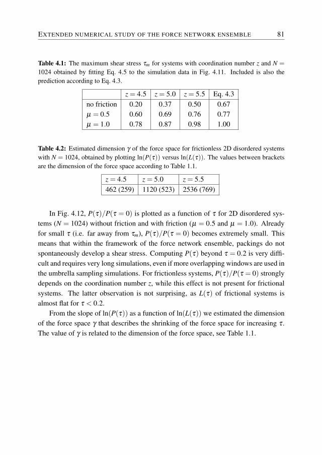
EXTENDED NUMERICAL STUDY OF THE FORCE NETWORK ENSEMBLE 81

Table 4.1: The maximum shear stress τm for systems with coordination number z and N =1024 obtained by fitting Eq. 4.5 to the simulation data in Fig. 4.11. Included is also theprediction according to Eq. 4.3.

z = 4.5 z = 5.0 z = 5.5 Eq. 4.3no friction 0.20 0.37 0.50 0.67µ = 0.5 0.60 0.69 0.76 0.77µ = 1.0 0.78 0.87 0.98 1.00

Table 4.2: Estimated dimension γ of the force space for frictionless 2D disordered systemswith N = 1024, obtained by plotting ln(P(τ)) versus ln(L(τ)). The values between bracketsare the dimension of the force space according to Table 1.1.

z = 4.5 z = 5.0 z = 5.5462 (259) 1120 (523) 2536 (769)

In Fig. 4.12, P(τ)/P(τ = 0) is plotted as a function of τ for 2D disordered sys-tems (N = 1024) without friction and with friction (µ = 0.5 and µ = 1.0). Alreadyfor small τ (i.e. far away from τm), P(τ)/P(τ = 0) becomes extremely small. Thismeans that within the framework of the force network ensemble, packings do notspontaneously develop a shear stress. Computing P(τ) beyond τ = 0.2 is very diffi-cult and requires very long simulations, even if more overlapping windows are used inthe umbrella sampling simulations. For frictionless systems, P(τ)/P(τ = 0) stronglydepends on the coordination number z, while this effect is not present for frictionalsystems. The latter observation is not surprising, as L(τ) of frictional systems isalmost flat for τ < 0.2.

From the slope of ln(P(τ)) as a function of ln(L(τ)) we estimated the dimensionof the force space γ that describes the shrinking of the force space for increasing τ .The value of γ is related to the dimension of the force space, see Table 1.1.

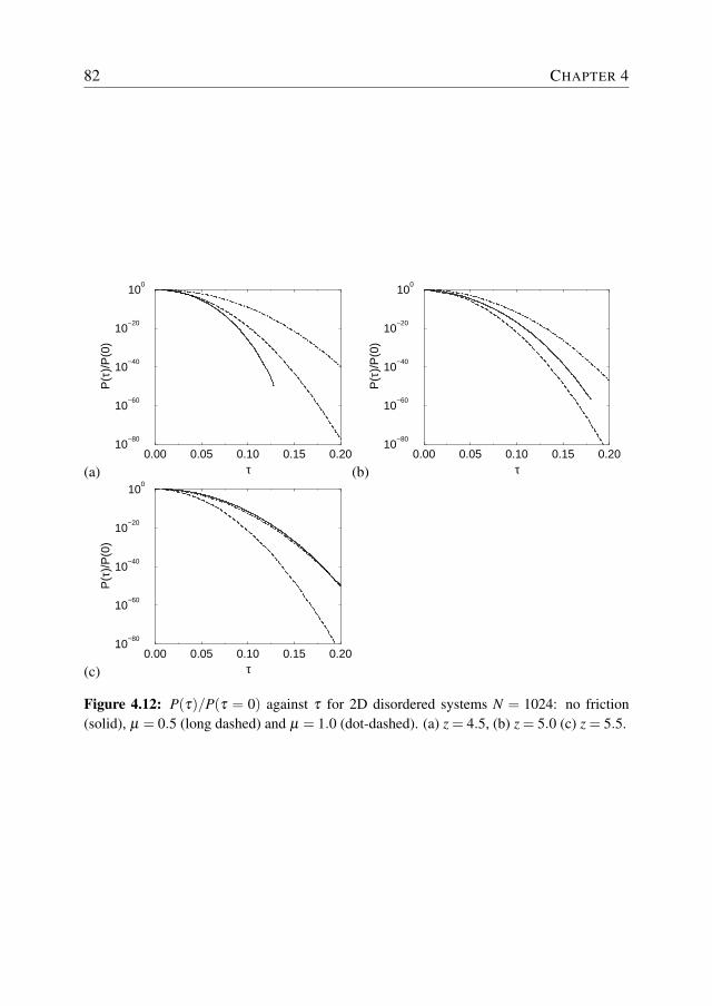
82 CHAPTER 4

(a)0.00 0.05 0.10 0.15 0.20

τ

10−80

10−60

10−40

10−20

100

P(τ

)/P

(0)

(b)0.00 0.05 0.10 0.15 0.20

τ

10−80

10−60

10−40

10−20

100

P(τ

)/P

(0)

(c)0.00 0.05 0.10 0.15 0.20

τ

10−80

10−60

10−40

10−20

100

P(τ

)/P

(0)

Figure 4.12: P(τ)/P(τ = 0) against τ for 2D disordered systems N = 1024: no friction(solid), µ = 0.5 (long dashed) and µ = 1.0 (dot-dashed). (a) z = 4.5, (b) z = 5.0 (c) z = 5.5.

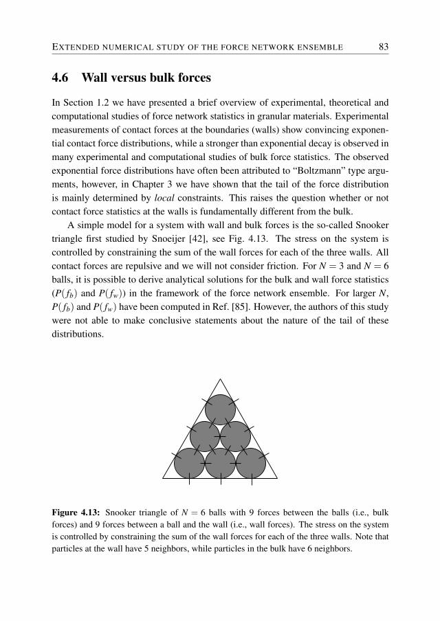
EXTENDED NUMERICAL STUDY OF THE FORCE NETWORK ENSEMBLE 83

4.6 Wall versus bulk forces

In Section 1.2 we have presented a brief overview of experimental, theoretical andcomputational studies of force network statistics in granular materials. Experimentalmeasurements of contact forces at the boundaries (walls) show convincing exponen-tial contact force distributions, while a stronger than exponential decay is observed inmany experimental and computational studies of bulk force statistics. The observedexponential force distributions have often been attributed to “Boltzmann” type argu-ments, however, in Chapter 3 we have shown that the tail of the force distributionis mainly determined by local constraints. This raises the question whether or notcontact force statistics at the walls is fundamentally different from the bulk.

A simple model for a system with wall and bulk forces is the so-called Snookertriangle first studied by Snoeijer [42], see Fig. 4.13. The stress on the system iscontrolled by constraining the sum of the wall forces for each of the three walls. Allcontact forces are repulsive and we will not consider friction. For N = 3 and N = 6balls, it is possible to derive analytical solutions for the bulk and wall force statistics(P( fb) and P( fw)) in the framework of the force network ensemble. For larger N,P( fb) and P( fw) have been computed in Ref. [85]. However, the authors of this studywere not able to make conclusive statements about the nature of the tail of thesedistributions.

Figure 4.13: Snooker triangle of N = 6 balls with 9 forces between the balls (i.e., bulkforces) and 9 forces between a ball and the wall (i.e., wall forces). The stress on the systemis controlled by constraining the sum of the wall forces for each of the three walls. Note thatparticles at the wall have 5 neighbors, while particles in the bulk have 6 neighbors.

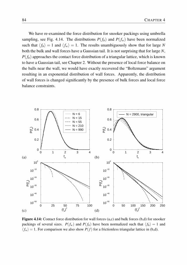
84 CHAPTER 4

We have re-examined the force distribution for snooker packings using umbrellasampling, see Fig. 4.14. The distributions P( fb) and P( fw) have been normalizedsuch that 〈 fb〉 = 1 and 〈 fw〉 = 1. The results unambiguously show that for large Nboth the bulk and wall forces have a Gaussian tail. It is not surprising that for large N,P( fb) approaches the contact force distribution of a triangular lattice, which is knownto have a Gaussian tail, see Chapter 2. Without the presence of local force balance onthe balls near the wall, we would have exactly recovered the “Boltzmann” argumentresulting in an exponential distribution of wall forces. Apparently, the distributionof wall forces is changed significantly by the presence of bulk forces and local forcebalance constraints.

(a)0 1 2 3 4

fw

0

0.2

0.4

0.6

0.8

P(f w)

N = 6N = 15N = 55N = 210N = 990

(b)0 1 2 3 4

fb

0

0.2

0.4

0.6

0.8P(

f b)

N = 2900, triangular

(c)0 25 50 75 100

(fw)2

10−50

10−40

10−30

10−20

10−10

100

P(f w)

(d)0 50 100 150 200 250

(fb)2

10−50

10−40

10−30

10−20

10−10

100

P(f b)

Figure 4.14: Contact force distribution for wall forces (a,c) and bulk forces (b,d) for snookerpackings of several sizes. P( fw) and P( fb) have been normalized such that 〈 fb〉 = 1 and〈 fw〉= 1. For comparison we also show P( f ) for a frictionless triangular lattice in (b,d).

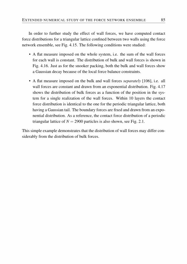
EXTENDED NUMERICAL STUDY OF THE FORCE NETWORK ENSEMBLE 85

In order to further study the effect of wall forces, we have computed contactforce distributions for a triangular lattice confined between two walls using the forcenetwork ensemble, see Fig. 4.15. The following conditions were studied:

• A flat measure imposed on the whole system, i.e. the sum of the wall forcesfor each wall is constant. The distribution of bulk and wall forces is shown inFig. 4.16. Just as for the snooker packing, both the bulk and wall forces showa Gaussian decay because of the local force balance constraints.

• A flat measure imposed on the bulk and wall forces separately [106], i.e. allwall forces are constant and drawn from an exponential distribution. Fig. 4.17shows the distribution of bulk forces as a function of the position in the sys-tem for a single realization of the wall forces. Within 10 layers the contactforce distribution is identical to the one for the periodic triangular lattice, bothhaving a Gaussian tail. The boundary forces are fixed and drawn from an expo-nential distribution. As a reference, the contact force distribution of a periodictriangular lattice of N = 2900 particles is also shown, see Fig. 2.1.

This simple example demonstrates that the distribution of wall forces may differ con-siderably from the distribution of bulk forces.

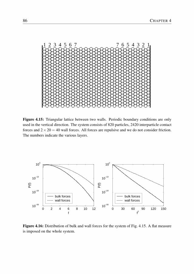
86 CHAPTER 4

1 2 3 4 5 6 7 7 6 5 4 3 2 1

Figure 4.15: Triangular lattice between two walls. Periodic boundary conditions are onlyused in the vertical direction. The system consists of 820 particles, 2420 interparticle contactforces and 2×20 = 40 wall forces. All forces are repulsive and we do not consider friction.The numbers indicate the various layers.

0 2 4 6 8 10 12f

10−30

10−20

10−10

100

P(f

)

bulk forceswall forces

0 30 60 90 120 150f2

10−30

10−20

10−10

100

P(f

)

bulk forceswall forces

Figure 4.16: Distribution of bulk and wall forces for the system of Fig. 4.15. A flat measureis imposed on the whole system.

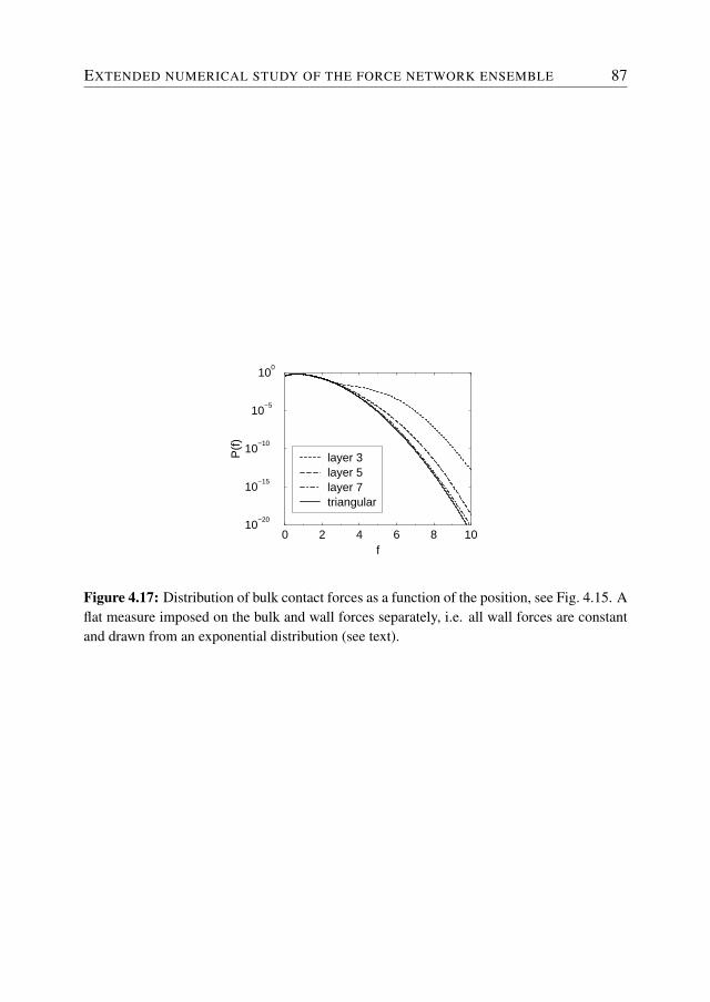
EXTENDED NUMERICAL STUDY OF THE FORCE NETWORK ENSEMBLE 87

0 2 4 6 8 10f

10−20

10−15

10−10

10−5

100

P(f

)

layer 3layer 5layer 7triangular

Figure 4.17: Distribution of bulk contact forces as a function of the position, see Fig. 4.15. Aflat measure imposed on the bulk and wall forces separately, i.e. all wall forces are constantand drawn from an exponential distribution (see text).

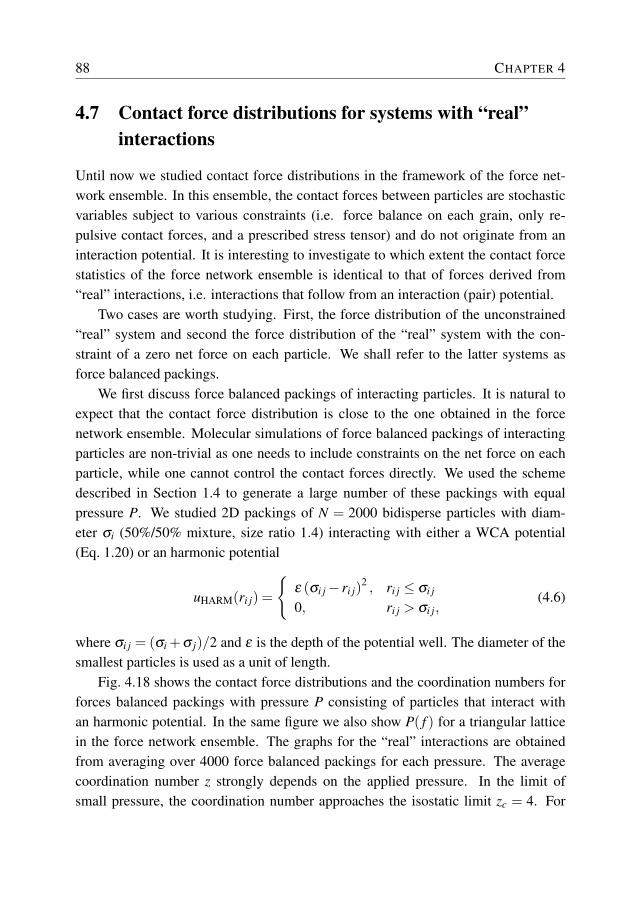
88 CHAPTER 4

4.7 Contact force distributions for systems with “real”interactions

Until now we studied contact force distributions in the framework of the force net-work ensemble. In this ensemble, the contact forces between particles are stochasticvariables subject to various constraints (i.e. force balance on each grain, only re-pulsive contact forces, and a prescribed stress tensor) and do not originate from aninteraction potential. It is interesting to investigate to which extent the contact forcestatistics of the force network ensemble is identical to that of forces derived from“real” interactions, i.e. interactions that follow from an interaction (pair) potential.

Two cases are worth studying. First, the force distribution of the unconstrained“real” system and second the force distribution of the “real” system with the con-straint of a zero net force on each particle. We shall refer to the latter systems asforce balanced packings.

We first discuss force balanced packings of interacting particles. It is natural toexpect that the contact force distribution is close to the one obtained in the forcenetwork ensemble. Molecular simulations of force balanced packings of interactingparticles are non-trivial as one needs to include constraints on the net force on eachparticle, while one cannot control the contact forces directly. We used the schemedescribed in Section 1.4 to generate a large number of these packings with equalpressure P. We studied 2D packings of N = 2000 bidisperse particles with diam-eter σi (50%/50% mixture, size ratio 1.4) interacting with either a WCA potential(Eq. 1.20) or an harmonic potential

uHARM(ri j) =

{ε (σi j− ri j)

2 , ri j ≤ σi j

0, ri j > σi j,(4.6)

where σi j = (σi +σ j)/2 and ε is the depth of the potential well. The diameter of thesmallest particles is used as a unit of length.

Fig. 4.18 shows the contact force distributions and the coordination numbers forforces balanced packings with pressure P consisting of particles that interact withan harmonic potential. In the same figure we also show P( f ) for a triangular latticein the force network ensemble. The graphs for the “real” interactions are obtainedfrom averaging over 4000 force balanced packings for each pressure. The averagecoordination number z strongly depends on the applied pressure. In the limit ofsmall pressure, the coordination number approaches the isostatic limit zc = 4. For

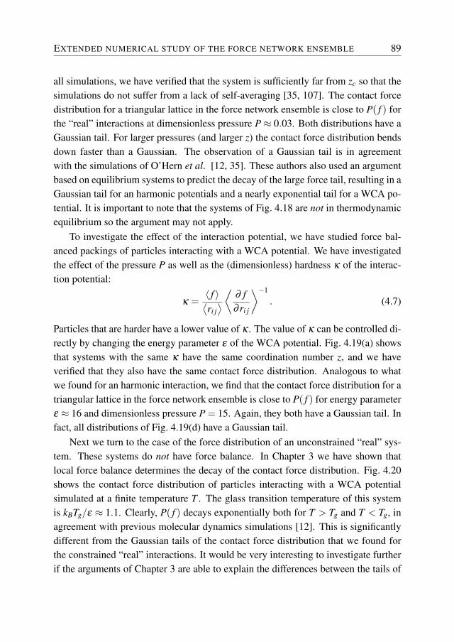
EXTENDED NUMERICAL STUDY OF THE FORCE NETWORK ENSEMBLE 89

all simulations, we have verified that the system is sufficiently far from zc so that thesimulations do not suffer from a lack of self-averaging [35, 107]. The contact forcedistribution for a triangular lattice in the force network ensemble is close to P( f ) forthe “real” interactions at dimensionless pressure P ≈ 0.03. Both distributions have aGaussian tail. For larger pressures (and larger z) the contact force distribution bendsdown faster than a Gaussian. The observation of a Gaussian tail is in agreementwith the simulations of O’Hern et al. [12, 35]. These authors also used an argumentbased on equilibrium systems to predict the decay of the large force tail, resulting in aGaussian tail for an harmonic potentials and a nearly exponential tail for a WCA po-tential. It is important to note that the systems of Fig. 4.18 are not in thermodynamicequilibrium so the argument may not apply.

To investigate the effect of the interaction potential, we have studied force bal-anced packings of particles interacting with a WCA potential. We have investigatedthe effect of the pressure P as well as the (dimensionless) hardness κ of the interac-tion potential:

κ =〈 f 〉⟨ri j⟩ ⟨ ∂ f

∂ ri j

⟩−1

. (4.7)

Particles that are harder have a lower value of κ . The value of κ can be controlled di-rectly by changing the energy parameter ε of the WCA potential. Fig. 4.19(a) showsthat systems with the same κ have the same coordination number z, and we haveverified that they also have the same contact force distribution. Analogous to whatwe found for an harmonic interaction, we find that the contact force distribution for atriangular lattice in the force network ensemble is close to P( f ) for energy parameterε ≈ 16 and dimensionless pressure P = 15. Again, they both have a Gaussian tail. Infact, all distributions of Fig. 4.19(d) have a Gaussian tail.

Next we turn to the case of the force distribution of an unconstrained “real” sys-tem. These systems do not have force balance. In Chapter 3 we have shown thatlocal force balance determines the decay of the contact force distribution. Fig. 4.20shows the contact force distribution of particles interacting with a WCA potentialsimulated at a finite temperature T . The glass transition temperature of this systemis kBTg/ε ≈ 1.1. Clearly, P( f ) decays exponentially both for T > Tg and T < Tg, inagreement with previous molecular dynamics simulations [12]. This is significantlydifferent from the Gaussian tails of the contact force distribution that we found forthe constrained “real” interactions. It would be very interesting to investigate furtherif the arguments of Chapter 3 are able to explain the differences between the tails of

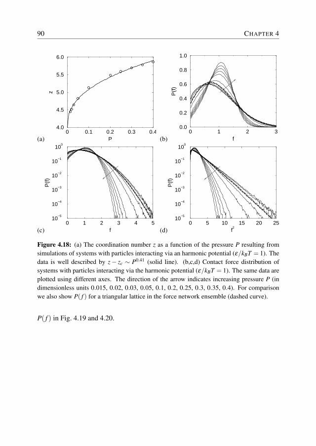
90 CHAPTER 4

(a)0 0.1 0.2 0.3 0.4

P

4.0

4.5

5.0

5.5

6.0z

(b)0 1 2 3

f

0.0

0.2

0.4

0.6

0.8

1.0

P(f

)

(c)0 1 2 3 4 5

f

10−5

10−4

10−3

10−2

10−1

100

P(f

)

(d)0 5 10 15 20 25

f2

10−5

10−4

10−3

10−2

10−1

100

P(f

)

Figure 4.18: (a) The coordination number z as a function of the pressure P resulting fromsimulations of systems with particles interacting via an harmonic potential (ε/kBT = 1). Thedata is well described by z− zc ∼ P0.41 (solid line). (b,c,d) Contact force distribution ofsystems with particles interacting via the harmonic potential (ε/kBT = 1). The same data areplotted using different axes. The direction of the arrow indicates increasing pressure P (indimensionless units 0.015, 0.02, 0.03, 0.05, 0.1, 0.2, 0.25, 0.3, 0.35, 0.4). For comparisonwe also show P( f ) for a triangular lattice in the force network ensemble (dashed curve).

P( f ) in Fig. 4.19 and 4.20.

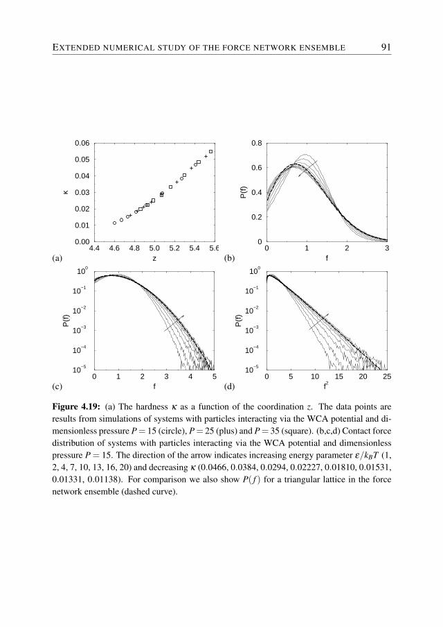
EXTENDED NUMERICAL STUDY OF THE FORCE NETWORK ENSEMBLE 91

(a)4.4 4.6 4.8 5.0 5.2 5.4 5.6

z

0.00

0.01

0.02

0.03

0.04

0.05

0.06

κ

(b)0 1 2 3

f

0

0.2

0.4

0.6

0.8

P(f

)

(c)0 1 2 3 4 5

f

10−5

10−4

10−3

10−2

10−1

100

P(f

)

(d)0 5 10 15 20 25

f2

10−5

10−4

10−3

10−2

10−1

100

P(f

)

Figure 4.19: (a) The hardness κ as a function of the coordination z. The data points areresults from simulations of systems with particles interacting via the WCA potential and di-mensionless pressure P = 15 (circle), P = 25 (plus) and P = 35 (square). (b,c,d) Contact forcedistribution of systems with particles interacting via the WCA potential and dimensionlesspressure P = 15. The direction of the arrow indicates increasing energy parameter ε/kBT (1,2, 4, 7, 10, 13, 16, 20) and decreasing κ (0.0466, 0.0384, 0.0294, 0.02227, 0.01810, 0.01531,0.01331, 0.01138). For comparison we also show P( f ) for a triangular lattice in the forcenetwork ensemble (dashed curve).

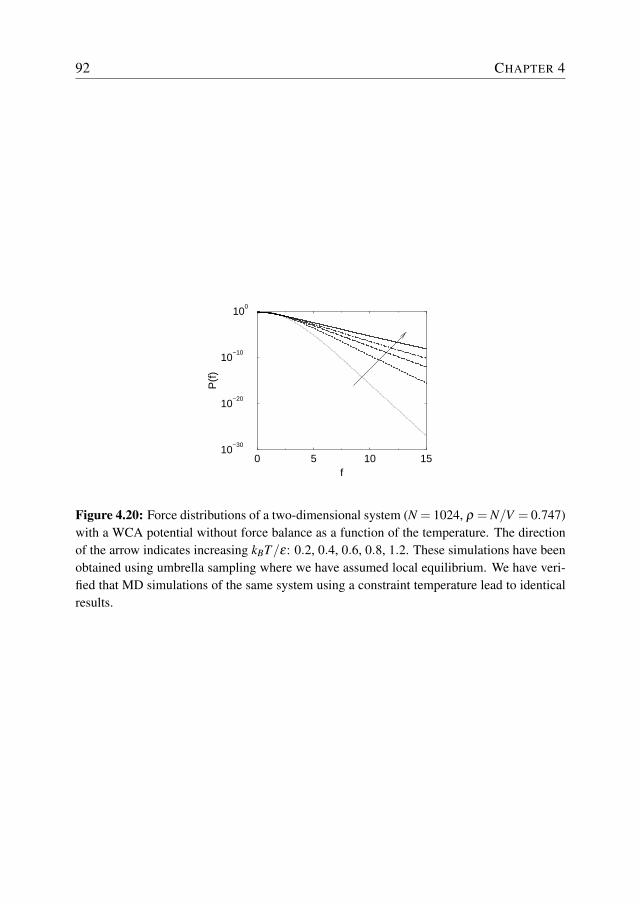
92 CHAPTER 4

0 5 10 15f

10−30

10−20

10−10

100

P(f)

Figure 4.20: Force distributions of a two-dimensional system (N = 1024, ρ = N/V = 0.747)with a WCA potential without force balance as a function of the temperature. The directionof the arrow indicates increasing kBT/ε: 0.2, 0.4, 0.6, 0.8, 1.2. These simulations have beenobtained using umbrella sampling where we have assumed local equilibrium. We have veri-fied that MD simulations of the same system using a constraint temperature lead to identicalresults.

References

[1] L. K. A. Dorren, A review of rockfall mechanics and modelling approaches,Prog. Phys. Geogr. 27, 69 (2003).

[2] S. De Toni and P. Scotton, Two-dimensional mathematical and numericalmodel for the dynamics of granular avalanches, Cold Regions Science andTechnology 43, 36 (2005).

[3] W. R. Ketterhagen, J. S. Curtis, C. R. Wassgren, and B. C. Hancock, Model-ing granular segregation in flow from quasi-three-dimensional, wedge-shapedhoppers, Powder Technol. 179, 126 (2008).

[4] F. Y. Fraige, P. A. Langston, and G. Z. Chen, Distinct element mod-elling of cubic particle packing and flow, Powder Technol. (in press,doi:10.1016/j.powtec.2007.12.009).

[5] E. DesRosiers Lachiver, N. Abatzoglou, L. Cartilier, and J. S. Simard, Ag-glomeration tendency in dry pharmaceutical granular systems, Eur. J. Pharm.Biopharm. 64, 193 (2006).

[6] K. Lee, T. Kim, P. Rajniak, and T. Matsoukas, Compositional distributions inmulticomponent aggregation, Chem. Eng. Sci. 63, 1293 (2008).

[7] M. van Hecke, Shape matters, Science 317, 49 (2007).

[8] M. van Hecke, Granular matter: A tale of tails, Science 435, 1041 (2005).

[9] H. P. Zhu, Z. Y. Zhou, R. Yang, and A. B. Yu, Discrete particle simulationof particulate systems: Theoretical developments, Chem. Eng. Sci. 62, 3378(2007).

[10] A. J. Liu and S. R. Nagel, Jamming is not just cool any more, Nature 396, 21(1998).

[11] J. H. Snoeijer, W. G. Ellenbroek, T. J. H. Vlugt, and M. van Hecke, Shearedforce-networks: anisotropies, yielding and geometry, Phys. Rev. Lett. 96,098001 (2006).

[12] C. S. O’Hern, S. A. Langer, A. J. Liu, and S. R. Nagel, Force distributionsnear jamming and glass transitions, Phys. Rev. Lett. 86, 111 (2001).

[13] L. E. Silbert, D. Ertas, G. S. Grest, H. T. C., and D. Levine, Analogies betweengranular jamming and the liquid-glass transition, Phys. Rev. E 65, 051307(2002).

[14] V. Trappe, V. Prasad, L. Cipelletti, P. N. Segre, and D. A. Weitz, Jammingphase diagram for attractive particles, Nature 411, 772 (2001).

[15] C. h. Liu, A. R. Nagel, D. A. Schecter, S. N. Coppersmith, S. Majumdar,O. Narayan, and T. A. Witten, Force fluctuations in bead packs, Science 269,513 (1995).

[16] http://www.roymech.co.uk/Useful_Tables/Tribology/co_of_frict.htm.

[17] F. Jones, H. Ryffel, E. Oberg, C. McCauley, and R. Heald, Machinery’s Hand-book, Industrial Press, 27th edition, 2004.

[18] H. M. Jaeger, S. R. Nagel, and R. P. Behringer, Granular solids, liquids, andgases, Rev. Mod. Phys. 68, 1259 (1996).

[19] P. G. de Gennes, Granular matter: a tentative view, Rev. Mod. Phys. 71, s374(1999).

[20] E. I. Corwin, H. M. Jaeger, and S. R. Nagel, Structural signature of jammingin granular media, Nature 435, 1075 (2005).

[21] D. M. Mueth, H. M. Jaeger, and S. R. Nagel, Force distribution in a granularmedium, Phys. Rev. E 57, 3164 (1998).

[22] D. L. Blair, N. W. Mueggenburg, A. H. Marshall, H. M. Jaeger, and S. R.Nagel, Force distributions in three-dimensional granular assemblies: Effectsof packing order and interparticle friction, Phys. Rev. E 63, 041304 (2001).

[23] J. M. Erikson, N. W. Mueggenburg, H. M. Jaeger, and S. R. Nagel, Forcedistributions in three-dimensional compressible granular packs, Phys. Rev. E66, 040301 (2002).

[24] G. Løvoll, K. J. Måløy, and E. G. Flekkøy, Force measurements on static gran-ular materials, Phys. Rev. E 60, 5872 (1999).

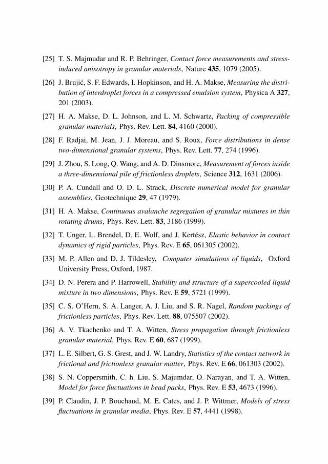
[25] T. S. Majmudar and R. P. Behringer, Contact force measurements and stress-induced anisotropy in granular materials, Nature 435, 1079 (2005).

[26] J. Brujic, S. F. Edwards, I. Hopkinson, and H. A. Makse, Measuring the distri-bution of interdroplet forces in a compressed emulsion system, Physica A 327,201 (2003).

[27] H. A. Makse, D. L. Johnson, and L. M. Schwartz, Packing of compressiblegranular materials, Phys. Rev. Lett. 84, 4160 (2000).

[28] F. Radjai, M. Jean, J. J. Moreau, and S. Roux, Force distributions in densetwo-dimensional granular systems, Phys. Rev. Lett. 77, 274 (1996).

[29] J. Zhou, S. Long, Q. Wang, and A. D. Dinsmore, Measurement of forces insidea three-dimensional pile of frictionless droplets, Science 312, 1631 (2006).

[30] P. A. Cundall and O. D. L. Strack, Discrete numerical model for granularassemblies, Geotechnique 29, 47 (1979).

[31] H. A. Makse, Continuous avalanche segregation of granular mixtures in thinrotating drums, Phys. Rev. Lett. 83, 3186 (1999).

[32] T. Unger, L. Brendel, D. E. Wolf, and J. Kertész, Elastic behavior in contactdynamics of rigid particles, Phys. Rev. E 65, 061305 (2002).

[33] M. P. Allen and D. J. Tildesley, Computer simulations of liquids, OxfordUniversity Press, Oxford, 1987.

[34] D. N. Perera and P. Harrowell, Stability and structure of a supercooled liquidmixture in two dimensions, Phys. Rev. E 59, 5721 (1999).

[35] C. S. O’Hern, S. A. Langer, A. J. Liu, and S. R. Nagel, Random packings offrictionless particles, Phys. Rev. Lett. 88, 075507 (2002).

[36] A. V. Tkachenko and T. A. Witten, Stress propagation through frictionlessgranular material, Phys. Rev. E 60, 687 (1999).

[37] L. E. Silbert, G. S. Grest, and J. W. Landry, Statistics of the contact network infrictional and frictionless granular matter, Phys. Rev. E 66, 061303 (2002).

[38] S. N. Coppersmith, C. h. Liu, S. Majumdar, O. Narayan, and T. A. Witten,Model for force fluctuations in bead packs, Phys. Rev. E 53, 4673 (1996).

[39] P. Claudin, J. P. Bouchaud, M. E. Cates, and J. P. Wittmer, Models of stressfluctuations in granular media, Phys. Rev. E 57, 4441 (1998).

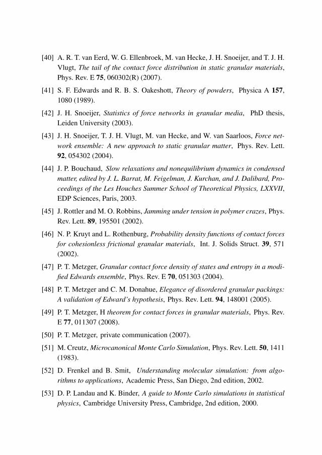
[40] A. R. T. van Eerd, W. G. Ellenbroek, M. van Hecke, J. H. Snoeijer, and T. J. H.Vlugt, The tail of the contact force distribution in static granular materials,Phys. Rev. E 75, 060302(R) (2007).

[41] S. F. Edwards and R. B. S. Oakeshott, Theory of powders, Physica A 157,1080 (1989).

[42] J. H. Snoeijer, Statistics of force networks in granular media, PhD thesis,Leiden University (2003).

[43] J. H. Snoeijer, T. J. H. Vlugt, M. van Hecke, and W. van Saarloos, Force net-work ensemble: A new approach to static granular matter, Phys. Rev. Lett.92, 054302 (2004).

[44] J. P. Bouchaud, Slow relaxations and nonequilibrium dynamics in condensedmatter, edited by J. L. Barrat, M. Feigelman, J. Kurchan, and J. Dalibard, Pro-ceedings of the Les Houches Summer School of Theoretical Physics, LXXVII,EDP Sciences, Paris, 2003.

[45] J. Rottler and M. O. Robbins, Jamming under tension in polymer crazes, Phys.Rev. Lett. 89, 195501 (2002).

[46] N. P. Kruyt and L. Rothenburg, Probability density functions of contact forcesfor cohesionless frictional granular materials, Int. J. Solids Struct. 39, 571(2002).

[47] P. T. Metzger, Granular contact force density of states and entropy in a modi-fied Edwards ensemble, Phys. Rev. E 70, 051303 (2004).

[48] P. T. Metzger and C. M. Donahue, Elegance of disordered granular packings:A validation of Edward’s hypothesis, Phys. Rev. Lett. 94, 148001 (2005).

[49] P. T. Metzger, H theorem for contact forces in granular materials, Phys. Rev.E 77, 011307 (2008).

[50] P. T. Metzger, private communication (2007).

[51] M. Creutz, Microcanonical Monte Carlo Simulation, Phys. Rev. Lett. 50, 1411(1983).

[52] D. Frenkel and B. Smit, Understanding molecular simulation: from algo-rithms to applications, Academic Press, San Diego, 2nd edition, 2002.

[53] D. P. Landau and K. Binder, A guide to Monte Carlo simulations in statisticalphysics, Cambridge University Press, Cambridge, 2nd edition, 2000.

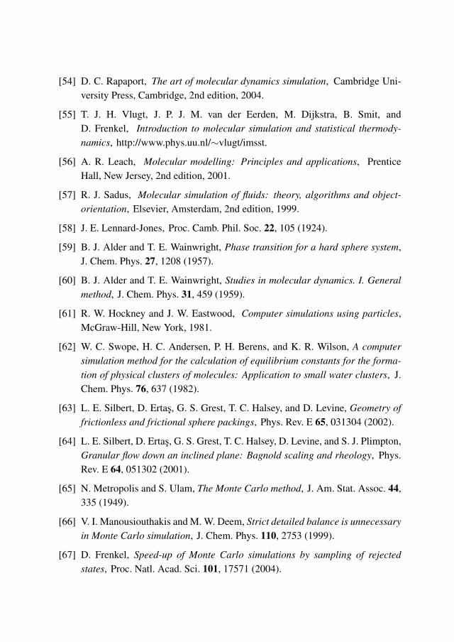
[54] D. C. Rapaport, The art of molecular dynamics simulation, Cambridge Uni-versity Press, Cambridge, 2nd edition, 2004.

[55] T. J. H. Vlugt, J. P. J. M. van der Eerden, M. Dijkstra, B. Smit, andD. Frenkel, Introduction to molecular simulation and statistical thermody-namics, http://www.phys.uu.nl/∼vlugt/imsst.

[56] A. R. Leach, Molecular modelling: Principles and applications, PrenticeHall, New Jersey, 2nd edition, 2001.

[57] R. J. Sadus, Molecular simulation of fluids: theory, algorithms and object-orientation, Elsevier, Amsterdam, 2nd edition, 1999.

[58] J. E. Lennard-Jones, Proc. Camb. Phil. Soc. 22, 105 (1924).

[59] B. J. Alder and T. E. Wainwright, Phase transition for a hard sphere system,J. Chem. Phys. 27, 1208 (1957).

[60] B. J. Alder and T. E. Wainwright, Studies in molecular dynamics. I. Generalmethod, J. Chem. Phys. 31, 459 (1959).

[61] R. W. Hockney and J. W. Eastwood, Computer simulations using particles,McGraw-Hill, New York, 1981.

[62] W. C. Swope, H. C. Andersen, P. H. Berens, and K. R. Wilson, A computersimulation method for the calculation of equilibrium constants for the forma-tion of physical clusters of molecules: Application to small water clusters, J.Chem. Phys. 76, 637 (1982).

[63] L. E. Silbert, D. Ertas, G. S. Grest, T. C. Halsey, and D. Levine, Geometry offrictionless and frictional sphere packings, Phys. Rev. E 65, 031304 (2002).

[64] L. E. Silbert, D. Ertas, G. S. Grest, T. C. Halsey, D. Levine, and S. J. Plimpton,Granular flow down an inclined plane: Bagnold scaling and rheology, Phys.Rev. E 64, 051302 (2001).

[65] N. Metropolis and S. Ulam, The Monte Carlo method, J. Am. Stat. Assoc. 44,335 (1949).

[66] V. I. Manousiouthakis and M. W. Deem, Strict detailed balance is unnecessaryin Monte Carlo simulation, J. Chem. Phys. 110, 2753 (1999).

[67] D. Frenkel, Speed-up of Monte Carlo simulations by sampling of rejectedstates, Proc. Natl. Acad. Sci. 101, 17571 (2004).

[68] N. Metropolis, A. W. Rosenbluth, M. N. Rosenbluth, A. H. Teller, andE. Teller, Equation of state calculations by fast computing machines, J. Chem.Phys. 21, 1087 (1953).

[69] G. M. Torrie and J. P. Valleau, Nonphysical sampling distributions in MonteCarlo free-energy estimation: umbrella sampling, J. Comp. Phys. 23, 187(1977).

[70] J. D. Weeks, D. Chandler, and H. C. Andersen, Role of repulsive forces indetermining the equilibrium structure of simple liquids, J. Chem. Phys. 54,5237 (1971).

[71] W. H. Press, S. A. Teukolsky, W. T. Vertterling, and B. P. Flannery, NumericalRecipes in Fortran 77: The art of scientific computing, Cambridge UniversityPress, Cambridge, 2nd edition, 1992.

[72] J. A. Snyman, A new and dynamic method for unconstrained minimization,Appl. Math. Modelling 6, 449 (1982).

[73] J. A. Snyman, An improved version of the original leapfrog dynamic methodfor unconstrained minimization: LFOP1(b), Appl. Math. Modelling 7, 216(1983).

[74] J. A. Snyman, A convergent dynamic method for large minimization problems,Comput. Math. Appl. 17, 1369 (1989).

[75] M. C. Payne, M. P. Teter, D. C. Allan, T. A. Arias, and J. D. Joannopoulos, It-erative minimization techniques for ab initio total-energy calculations: Molec-ular dynamics and conjugate gradients, Rev. Mod. Phys. 64, 1045 (1992).

[76] J. Baker, An algorithm for the location of transition states, J. Comp. Chem. 7,385 (1986).

[77] K. Bagi, Statistical analysis of contact force components in random granularassemblies, Granular Matter 5, 45 (2003).

[78] J. P. J. M. van der Eerden, J. Makkinje, and T. J. H. Vlugt, Local order ininterfaces, J. Cryst. Growth 275, 83 (2004).

[79] T. Unger, J. Kertész, and D. E. Wolf, Force Indeterminacy in the Jammed Stateof Hard Disks, Phys. Rev. Lett. 94, 178001 (2005).

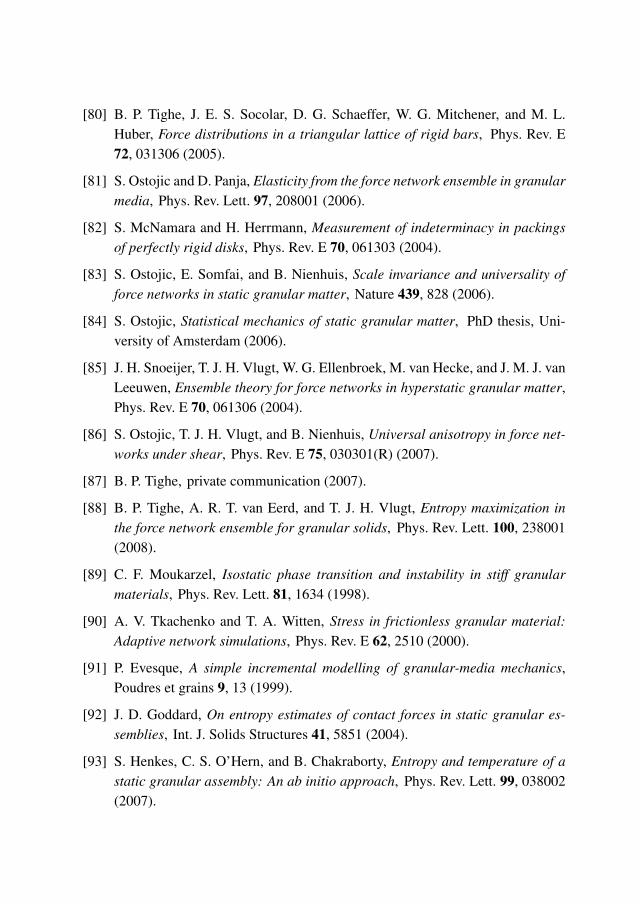
[80] B. P. Tighe, J. E. S. Socolar, D. G. Schaeffer, W. G. Mitchener, and M. L.Huber, Force distributions in a triangular lattice of rigid bars, Phys. Rev. E72, 031306 (2005).

[81] S. Ostojic and D. Panja, Elasticity from the force network ensemble in granularmedia, Phys. Rev. Lett. 97, 208001 (2006).

[82] S. McNamara and H. Herrmann, Measurement of indeterminacy in packingsof perfectly rigid disks, Phys. Rev. E 70, 061303 (2004).

[83] S. Ostojic, E. Somfai, and B. Nienhuis, Scale invariance and universality offorce networks in static granular matter, Nature 439, 828 (2006).

[84] S. Ostojic, Statistical mechanics of static granular matter, PhD thesis, Uni-versity of Amsterdam (2006).

[85] J. H. Snoeijer, T. J. H. Vlugt, W. G. Ellenbroek, M. van Hecke, and J. M. J. vanLeeuwen, Ensemble theory for force networks in hyperstatic granular matter,Phys. Rev. E 70, 061306 (2004).

[86] S. Ostojic, T. J. H. Vlugt, and B. Nienhuis, Universal anisotropy in force net-works under shear, Phys. Rev. E 75, 030301(R) (2007).

[87] B. P. Tighe, private communication (2007).

[88] B. P. Tighe, A. R. T. van Eerd, and T. J. H. Vlugt, Entropy maximization inthe force network ensemble for granular solids, Phys. Rev. Lett. 100, 238001(2008).

[89] C. F. Moukarzel, Isostatic phase transition and instability in stiff granularmaterials, Phys. Rev. Lett. 81, 1634 (1998).

[90] A. V. Tkachenko and T. A. Witten, Stress in frictionless granular material:Adaptive network simulations, Phys. Rev. E 62, 2510 (2000).

[91] P. Evesque, A simple incremental modelling of granular-media mechanics,Poudres et grains 9, 13 (1999).

[92] J. D. Goddard, On entropy estimates of contact forces in static granular es-semblies, Int. J. Solids Structures 41, 5851 (2004).

[93] S. Henkes, C. S. O’Hern, and B. Chakraborty, Entropy and temperature of astatic granular assembly: An ab initio approach, Phys. Rev. Lett. 99, 038002(2007).

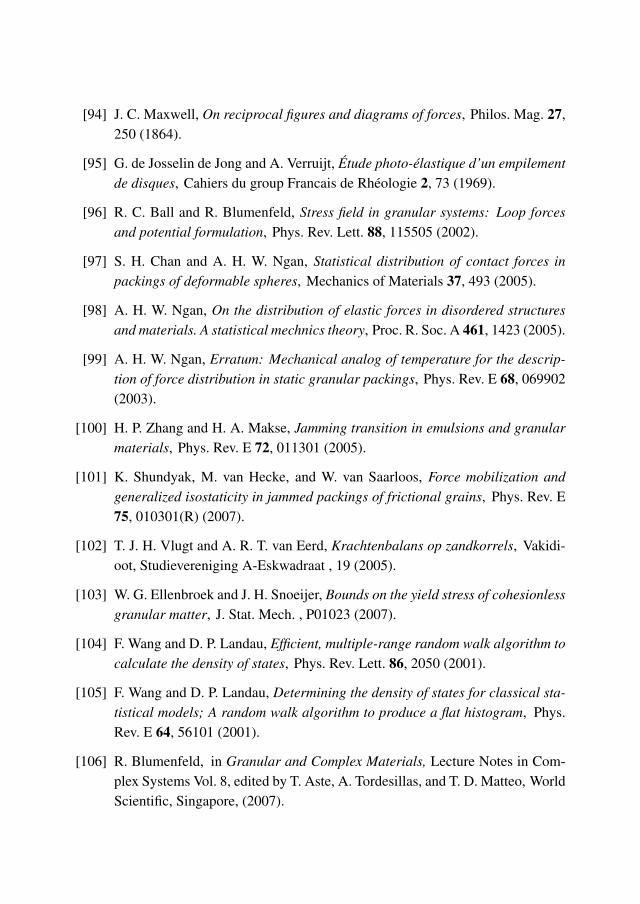
[94] J. C. Maxwell, On reciprocal figures and diagrams of forces, Philos. Mag. 27,250 (1864).

[95] G. de Josselin de Jong and A. Verruijt, Étude photo-élastique d’un empilementde disques, Cahiers du group Francais de Rhéologie 2, 73 (1969).

[96] R. C. Ball and R. Blumenfeld, Stress field in granular systems: Loop forcesand potential formulation, Phys. Rev. Lett. 88, 115505 (2002).

[97] S. H. Chan and A. H. W. Ngan, Statistical distribution of contact forces inpackings of deformable spheres, Mechanics of Materials 37, 493 (2005).

[98] A. H. W. Ngan, On the distribution of elastic forces in disordered structuresand materials. A statistical mechnics theory, Proc. R. Soc. A 461, 1423 (2005).

[99] A. H. W. Ngan, Erratum: Mechanical analog of temperature for the descrip-tion of force distribution in static granular packings, Phys. Rev. E 68, 069902(2003).

[100] H. P. Zhang and H. A. Makse, Jamming transition in emulsions and granularmaterials, Phys. Rev. E 72, 011301 (2005).

[101] K. Shundyak, M. van Hecke, and W. van Saarloos, Force mobilization andgeneralized isostaticity in jammed packings of frictional grains, Phys. Rev. E75, 010301(R) (2007).

[102] T. J. H. Vlugt and A. R. T. van Eerd, Krachtenbalans op zandkorrels, Vakidi-oot, Studievereniging A-Eskwadraat , 19 (2005).

[103] W. G. Ellenbroek and J. H. Snoeijer, Bounds on the yield stress of cohesionlessgranular matter, J. Stat. Mech. , P01023 (2007).

[104] F. Wang and D. P. Landau, Efficient, multiple-range random walk algorithm tocalculate the density of states, Phys. Rev. Lett. 86, 2050 (2001).

[105] F. Wang and D. P. Landau, Determining the density of states for classical sta-tistical models; A random walk algorithm to produce a flat histogram, Phys.Rev. E 64, 56101 (2001).

[106] R. Blumenfeld, in Granular and Complex Materials, Lecture Notes in Com-plex Systems Vol. 8, edited by T. Aste, A. Tordesillas, and T. D. Matteo, WorldScientific, Singapore, (2007).

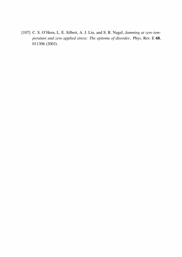
[107] C. S. O’Hern, L. E. Silbert, A. J. Liu, and S. R. Nagel, Jamming at zero tem-perature and zero applied stress: The epitome of disorder, Phys. Rev. E 68,011306 (2003).

Summary

Granular materials such as sand and grains of corn have both liquid-like and solid-likeproperties similar to both liquids and solids. Dry sand in an hour-glass can flow justlike water, while sand in a sand castle closely resembles a solid. Because of theseinteresting properties granular matter has received much attention from numerousphysicists. Part of the research on these materials focuses on the statistics of contactforces between individual particles (grains) and how these statistics can be used tounderstand and predict material properties. Contact forces in granular materials areorganized in so-called forces networks. The magnitude of the contact forces may varyconsiderably. Some particles experience contact forces much larger than the averagecontact force, see for example Fig. 1.2 and 1.8 of this thesis. The presence of manylarge contact forces in a sand pile may result in yielding, i.e. breaking down of thesand pile. A common quantity to characterize these force variations is the probabilitydistribution P( f ) of the contact force f between two particles. Usually, the contactforce distribution of a static system has its maximum near the average force 〈 f 〉, seefor example Fig. 1.1 of this thesis.

A long-standing issue in the area of granular media is the asymptotic behaviorof the contact force distribution P( f ) for large forces. In particular, one discusseswhether the tail of P( f ) is exponential, Gaussian, or has a different form. Further-more, its relation with material and system properties is under scruteny. In a recentissue of Nature (volume 435, 23 June 2005) three papers pay attention to this subject.Two different experimental methods are often applied to determine contact forces instatic granular materials. The first measures boundary forces using carbon paper. Theforce between grains and the wall of the container, that holds the grains, is deducedfrom imprints on carbon paper. For large boundary forces the measured distributiondecays exponentially. This observation is often used to suggest an analogy with theBoltzmann distribution of the microcanonical ensemble. In this ensemble, N randomvariables xi satisfy the constraints ∑

Ni=1 xi = N 〈x〉 and xi ≥ 0. In the thermodynamic

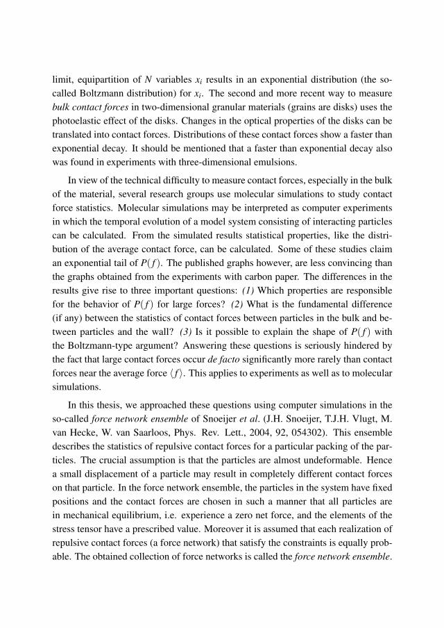
limit, equipartition of N variables xi results in an exponential distribution (the so-called Boltzmann distribution) for xi. The second and more recent way to measurebulk contact forces in two-dimensional granular materials (grains are disks) uses thephotoelastic effect of the disks. Changes in the optical properties of the disks can betranslated into contact forces. Distributions of these contact forces show a faster thanexponential decay. It should be mentioned that a faster than exponential decay alsowas found in experiments with three-dimensional emulsions.

In view of the technical difficulty to measure contact forces, especially in the bulkof the material, several research groups use molecular simulations to study contactforce statistics. Molecular simulations may be interpreted as computer experimentsin which the temporal evolution of a model system consisting of interacting particlescan be calculated. From the simulated results statistical properties, like the distri-bution of the average contact force, can be calculated. Some of these studies claiman exponential tail of P( f ). The published graphs however, are less convincing thanthe graphs obtained from the experiments with carbon paper. The differences in theresults give rise to three important questions: (1) Which properties are responsiblefor the behavior of P( f ) for large forces? (2) What is the fundamental difference(if any) between the statistics of contact forces between particles in the bulk and be-tween particles and the wall? (3) Is it possible to explain the shape of P( f ) withthe Boltzmann-type argument? Answering these questions is seriously hindered bythe fact that large contact forces occur de facto significantly more rarely than contactforces near the average force 〈 f 〉. This applies to experiments as well as to molecularsimulations.

In this thesis, we approached these questions using computer simulations in theso-called force network ensemble of Snoeijer et al. (J.H. Snoeijer, T.J.H. Vlugt, M.van Hecke, W. van Saarloos, Phys. Rev. Lett., 2004, 92, 054302). This ensembledescribes the statistics of repulsive contact forces for a particular packing of the par-ticles. The crucial assumption is that the particles are almost undeformable. Hencea small displacement of a particle may result in completely different contact forceson that particle. In the force network ensemble, the particles in the system have fixedpositions and the contact forces are chosen in such a manner that all particles arein mechanical equilibrium, i.e. experience a zero net force, and the elements of thestress tensor have a prescribed value. Moreover it is assumed that each realization ofrepulsive contact forces (a force network) that satisfy the constraints is equally prob-able. The obtained collection of force networks is called the force network ensemble.

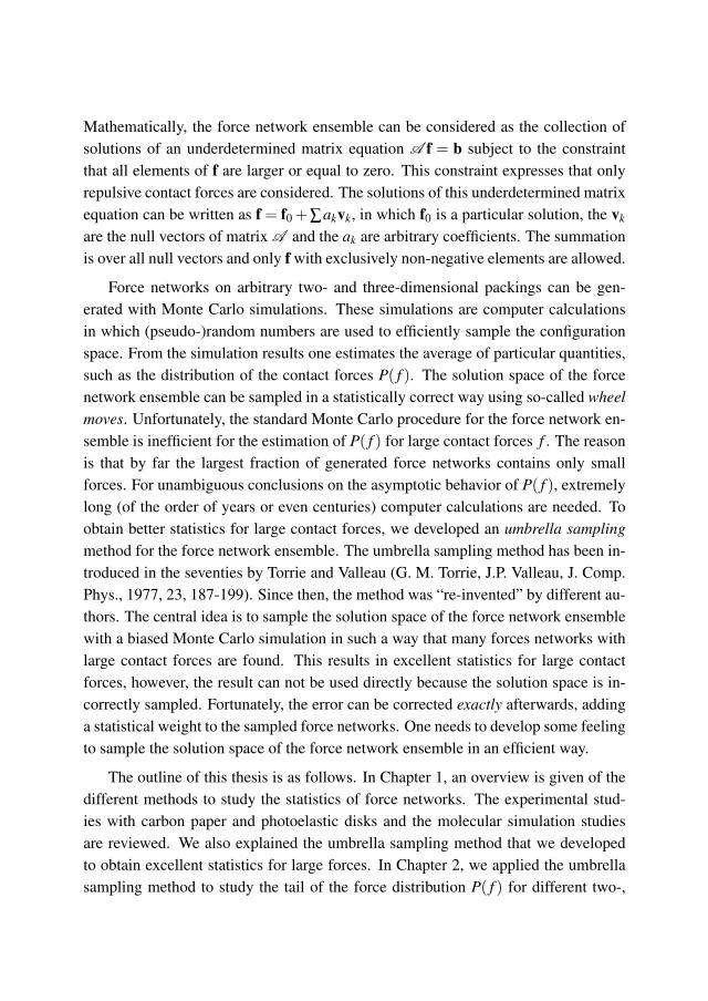
Mathematically, the force network ensemble can be considered as the collection ofsolutions of an underdetermined matrix equation A f = b subject to the constraintthat all elements of f are larger or equal to zero. This constraint expresses that onlyrepulsive contact forces are considered. The solutions of this underdetermined matrixequation can be written as f = f0 +∑akvk, in which f0 is a particular solution, the vk

are the null vectors of matrix A and the ak are arbitrary coefficients. The summationis over all null vectors and only f with exclusively non-negative elements are allowed.

Force networks on arbitrary two- and three-dimensional packings can be gen-erated with Monte Carlo simulations. These simulations are computer calculationsin which (pseudo-)random numbers are used to efficiently sample the configurationspace. From the simulation results one estimates the average of particular quantities,such as the distribution of the contact forces P( f ). The solution space of the forcenetwork ensemble can be sampled in a statistically correct way using so-called wheelmoves. Unfortunately, the standard Monte Carlo procedure for the force network en-semble is inefficient for the estimation of P( f ) for large contact forces f . The reasonis that by far the largest fraction of generated force networks contains only smallforces. For unambiguous conclusions on the asymptotic behavior of P( f ), extremelylong (of the order of years or even centuries) computer calculations are needed. Toobtain better statistics for large contact forces, we developed an umbrella samplingmethod for the force network ensemble. The umbrella sampling method has been in-troduced in the seventies by Torrie and Valleau (G. M. Torrie, J.P. Valleau, J. Comp.Phys., 1977, 23, 187-199). Since then, the method was “re-invented” by different au-thors. The central idea is to sample the solution space of the force network ensemblewith a biased Monte Carlo simulation in such a way that many forces networks withlarge contact forces are found. This results in excellent statistics for large contactforces, however, the result can not be used directly because the solution space is in-correctly sampled. Fortunately, the error can be corrected exactly afterwards, addinga statistical weight to the sampled force networks. One needs to develop some feelingto sample the solution space of the force network ensemble in an efficient way.

The outline of this thesis is as follows. In Chapter 1, an overview is given of thedifferent methods to study the statistics of force networks. The experimental stud-ies with carbon paper and photoelastic disks and the molecular simulation studiesare reviewed. We also explained the umbrella sampling method that we developedto obtain excellent statistics for large forces. In Chapter 2, we applied the umbrellasampling method to study the tail of the force distribution P( f ) for different two-,

three- and four-dimensional systems. The average number of contacts z of a parti-cle and the packing configuration are shown not to be important for the asymptoticbehavior of P( f ). Only the dimensionality of the system has a significant influ-ence: P( f ) ∼ exp[−c f α ] with α ≈ 2.0 for two-dimensional systems, α ≈ 1.7 forthree-dimensional systems and α ≈ 1.4 for four-dimensional systems. In Chapter 3,a possible explanation is found for the Gaussian decay of large contact forces intwo-dimensional systems. It was found that mechanical balance on each particle isessential for the tail of the contact force distribution. Under this constraint maximiz-ing the entropy results in a contact force distribution with a generic Gaussian tail.This distribution is almost in perfect agreement with the umbrella sampling simula-tions for systems with and without friction, both for triangular and for square lattices.Removing the mechanical equilibrium constraint on each particle, maximization ofthe entropy results in an exponential tail of P( f ). This is consistent with the “Boltz-mann” argument. We conclude that the tail of P( f ) is determined by local mechanicalequilibrium, which throws serious doubts on the statement that exponential statisticsare a generic property of static granular materials. In Chapter 4, several aspects arehighlighted. We show that in the presence of shear stress P( f ) is strongly directiondependent. As a result the tail of the orientation-averaged P( f ) may look (partly)exponential even though for each individual direction the tail is Gaussian. We de-velop methods to find the maximum possible force in a system and to determine thedimension of the force space. We demonstrate that the wall-contact force distributionmay differ essentially from the bulk-contact force distribution. This chapter endswith a detailed comparison between P( f ) in the force network ensemble and P( f )from molecular simulations of particles with a “real” pair interaction. We show thatthese distributions are different in general. Nevertheless our preliminary calculationssuggest that applying the constraint of local mechanical equilibrium, the force distri-bution of the “real” system crosses over towards the distribution of the force networkensemble.

Samenvatting

Granulaire materialen zoals zand en graankorrels hebben eigenschappen overeenkom-stig met zowel vloeistoffen als vaste stoffen. Zo kan droog zand in een zandlopernet als water stromen, terwijl zand in zandkasteel juist meer op een vaste stof lijkt.Door deze bijzondere eigenschappen staan granulaire materialen in de belangstellingbij natuurkundigen. Een deel van het onderzoek naar deze materialen richt zichop de statistiek van contactkrachten tussen individuele deeltjes (zandkorrels) en hoemen deze kan gebruiken om eigenschappen van materialen te begrijpen en te voor-spellen. Contactkrachten in granulaire materialen zijn georganiseerd in zogenaamdekrachtennetwerken. De grootte van deze krachten kan sterk variëren over de ruimte.Sommige korrels ondervinden bijvoorbeeld contactkrachten die veel groter zijn dande gemiddelde contactkracht, zie bijvoorbeeld Fig. 1.2 en 1.8 van dit proefschrift.De aanwezigheid van veel grote contactkrachten in een zandhoop, al dan niet veroor-zaakt door een externe kracht, kan de zandhoop doen instorten. Een veelgebruiktegrootheid om krachtennetwerken te karakteriseren is de kansverdeling P( f ) van decontactkracht f tussen twee korrels. Voor stilstaande systemen heeft deze verde-ling vaak een maximum in de buurt van de gemiddelde kracht 〈 f 〉, zie bijvoorbeeldFig. 1.1 van dit proefschrift.

Het asymptotisch gedrag van de contactkrachtverdeling P( f ) voor granulaire ma-terialen staat momenteel ter discussie. Een van de centrale vragen is of de P( f ) voorgrote f (de staart) een exponentiële, Gaussische, dan wel een andere vorm heeft.Verder wordt de relatie tussen P( f ) en materiaal- en systeemeigenschappen onder-zocht. In een recent nummer van het toonaangevende blad Nature (volume 435, 23juni 2005) besteden maar liefst drie artikelen aandacht aan dit onderwerp. Tweeverschillende experimentele methoden worden vaak gebruikt om contactkrachten instatische (in rust zijnde) granulaire materialen te bepalen. Bij de eerste methode ge-bruikt men carbonpapier om de grootte van de wandcontactkrachten te meten tussenkorrels en de wand van de container waar het materiaal zich in bevindt. De afdrukken

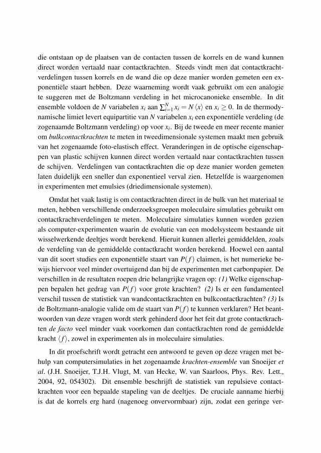
die ontstaan op de plaatsen van de contacten tussen de korrels en de wand kunnendirect worden vertaald naar contactkrachten. Steeds vindt men dat contactkracht-verdelingen tussen korrels en de wand die op deze manier worden gemeten een ex-ponentiële staart hebben. Deze waarneming wordt vaak gebruikt om een analogiete suggeren met de Boltzmann verdeling in het microcanonieke ensemble. In ditensemble voldoen de N variabelen xi aan ∑

Ni=1 xi = N 〈x〉 en xi ≥ 0. In de thermody-

namische limiet levert equipartitie van N variabelen xi een exponentiële verdeling (dezogenaamde Boltzmann verdeling) op voor xi. Bij de tweede en meer recente manierom bulkcontactkrachten te meten in tweedimensionale systemen maakt men gebruikvan het zogenaamde foto-elastisch effect. Veranderingen in de optische eigenschap-pen van plastic schijven kunnen direct worden vertaald naar contactkrachten tussende schijven. Verdelingen van contactkrachten die op deze manier worden gemetenlaten duidelijk een sneller dan exponentieel verval zien. Hetzelfde is waargenomenin experimenten met emulsies (driedimensionale systemen).

Omdat het vaak lastig is om contactkrachten direct in de bulk van het materiaal temeten, hebben verschillende onderzoeksgroepen moleculaire simulaties gebruikt omcontactkrachtverdelingen te meten. Moleculaire simulaties kunnen worden gezienals computer-experimenten waarin de evolutie van een modelsysteem bestaande uitwisselwerkende deeltjes wordt berekend. Hieruit kunnen allerlei gemiddelden, zoalsde verdeling van de gemiddelde contactkracht worden berekend. Hoewel een aantalvan dit soort studies een exponentiële staart van P( f ) claimen, is het numerieke be-wijs hiervoor veel minder overtuigend dan bij de experimenten met carbonpapier. Deverschillen in de resultaten roepen drie belangrijke vragen op: (1) Welke eigenschap-pen bepalen het gedrag van P( f ) voor grote krachten? (2) Is er een fundamenteelverschil tussen de statistiek van wandcontactkrachten en bulkcontactkrachten? (3) Isde Boltzmann-analogie valide om de staart van P( f ) te kunnen verklaren? Het beant-woorden van deze vragen wordt sterk gehinderd door het feit dat grote contactkrach-ten de facto veel minder vaak voorkomen dan contactkrachten rond de gemiddeldekracht 〈 f 〉, zowel in experimenten als in moleculaire simulaties.

In dit proefschrift wordt getracht een antwoord te geven op deze vragen met be-hulp van computersimulaties in het zogenaamde krachten-ensemble van Snoeijer etal. (J.H. Snoeijer, T.J.H. Vlugt, M. van Hecke, W. van Saarloos, Phys. Rev. Lett.,2004, 92, 054302). Dit ensemble beschrijft de statistiek van repulsieve contact-krachten voor een bepaalde stapeling van de deeltjes. De cruciale aanname hierbijis dat de korrels erg hard (nagenoeg onvervormbaar) zijn, zodat een geringe ver-

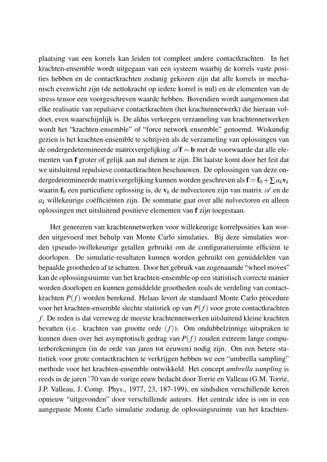
plaatsing van een korrels kan leiden tot compleet andere contactkrachten. In hetkrachten-ensemble wordt uitgegaan van een systeem waarbij de korrels vaste posi-ties hebben en de contactkrachten zodanig gekozen zijn dat alle korrels in mecha-nisch evenwicht zijn (de nettokracht op iedere korrel is nul) en de elementen van destress tensor een voorgeschreven waarde hebben. Bovendien wordt aangenomen datelke realisatie van repulsieve contactkrachten (het krachtennetwerk) die hieraan vol-doet, even waarschijnlijk is. De aldus verkregen verzameling van krachtennetwerkenwordt het “krachten-ensemble” of “force network ensemble” genoemd. Wiskundiggezien is het krachten-ensemble te schrijven als de verzameling van oplossingen vande ondergedetermineerde matrixvergelijking A f = b met de voorwaarde dat alle ele-menten van f groter of gelijk aan nul dienen te zijn. Dit laatste komt door het feit datwe uitsluitend repulsieve contactkrachten beschouwen. De oplossingen van deze on-dergedetermineerde matrixvergelijking kunnen worden geschreven als f = f0 +∑akvk

waarin f0 een particuliere oplossing is, de vk de nulvectoren zijn van matrix A en deak willekeurige coëfficiënten zijn. De sommatie gaat over alle nulvectoren en alleenoplossingen met uitsluitend positieve elementen van f zijn toegestaan.

Het genereren van krachtennetwerken voor willekeurige korrelposities kan wor-den uitgevoerd met behulp van Monte Carlo simulaties. Bij deze simulaties wor-den (pseudo-)willekeurige getallen gebruikt om de configuratieruimte efficiënt tedoorlopen. De simulatie-resultaten kunnen worden gebruikt om gemiddelden vanbepaalde grootheden af te schatten. Door het gebruik van zogenaamde “wheel moves”kan de oplossingsruimte van het krachten-ensemble op een statistisch correcte manierworden doorlopen en kunnen gemiddelde grootheden zoals de verdeling van contact-krachten P( f ) worden berekend. Helaas levert de standaard Monte Carlo procedurevoor het krachten-ensemble slechte statistiek op van P( f ) voor grote contactkrachtenf . De reden is dat verreweg de meeste krachtennetwerken uitsluitend kleine krachtenbevatten (i.e. krachten van grootte orde 〈 f 〉). Om ondubbelzinnige uitspraken tekunnen doen over het asymptotisch gedrag van P( f ) zouden extreem lange compu-terberekeningen (in de orde van jaren tot eeuwen) nodig zijn. Om een betere sta-tistiek voor grote contactkrachten te verkrijgen hebben we een “umbrella sampling”methode voor het krachten-ensemble ontwikkeld. Het concept umbrella sampling isreeds in de jaren ’70 van de vorige eeuw bedacht door Torrie en Valleau (G.M. Torrie,J.P. Valleau, J. Comp. Phys., 1977, 23, 187-199), en sindsdien verschillende kerenopnieuw “uitgevonden” door verschillende auteurs. Het centrale idee is om in eenaangepaste Monte Carlo simulatie zodanig de oplossingsruimte van het krachten-

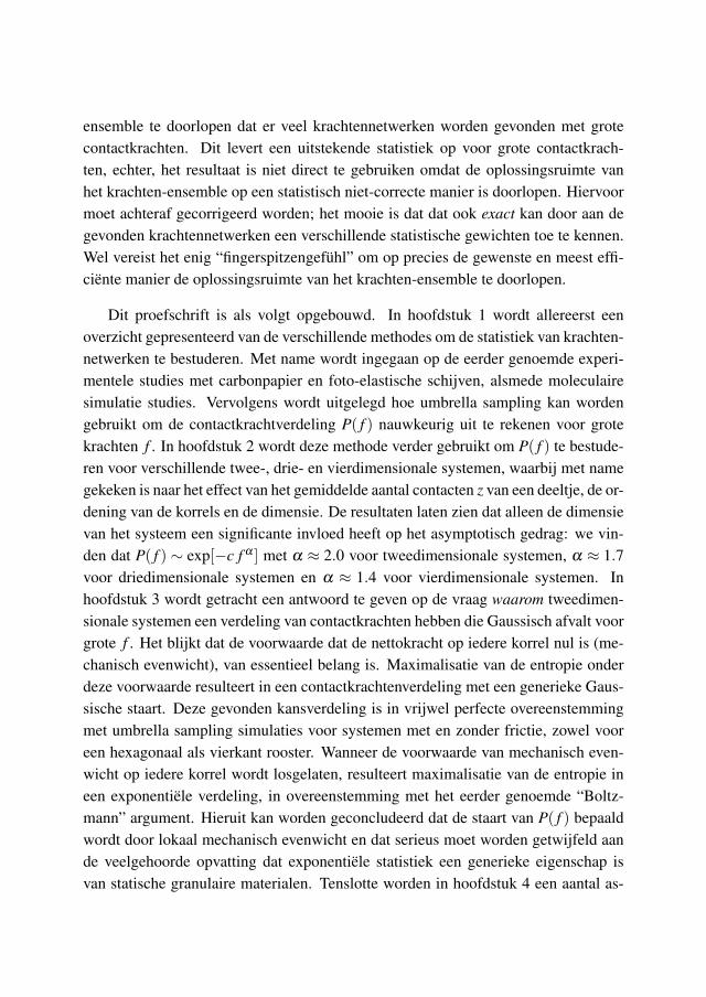
ensemble te doorlopen dat er veel krachtennetwerken worden gevonden met grotecontactkrachten. Dit levert een uitstekende statistiek op voor grote contactkrach-ten, echter, het resultaat is niet direct te gebruiken omdat de oplossingsruimte vanhet krachten-ensemble op een statistisch niet-correcte manier is doorlopen. Hiervoormoet achteraf gecorrigeerd worden; het mooie is dat dat ook exact kan door aan degevonden krachtennetwerken een verschillende statistische gewichten toe te kennen.Wel vereist het enig “fingerspitzengefühl” om op precies de gewenste en meest effi-ciënte manier de oplossingsruimte van het krachten-ensemble te doorlopen.

Dit proefschrift is als volgt opgebouwd. In hoofdstuk 1 wordt allereerst eenoverzicht gepresenteerd van de verschillende methodes om de statistiek van krachten-netwerken te bestuderen. Met name wordt ingegaan op de eerder genoemde experi-mentele studies met carbonpapier en foto-elastische schijven, alsmede moleculairesimulatie studies. Vervolgens wordt uitgelegd hoe umbrella sampling kan wordengebruikt om de contactkrachtverdeling P( f ) nauwkeurig uit te rekenen voor grotekrachten f . In hoofdstuk 2 wordt deze methode verder gebruikt om P( f ) te bestude-ren voor verschillende twee-, drie- en vierdimensionale systemen, waarbij met namegekeken is naar het effect van het gemiddelde aantal contacten z van een deeltje, de or-dening van de korrels en de dimensie. De resultaten laten zien dat alleen de dimensievan het systeem een significante invloed heeft op het asymptotisch gedrag: we vin-den dat P( f ) ∼ exp[−c f α ] met α ≈ 2.0 voor tweedimensionale systemen, α ≈ 1.7voor driedimensionale systemen en α ≈ 1.4 voor vierdimensionale systemen. Inhoofdstuk 3 wordt getracht een antwoord te geven op de vraag waarom tweedimen-sionale systemen een verdeling van contactkrachten hebben die Gaussisch afvalt voorgrote f . Het blijkt dat de voorwaarde dat de nettokracht op iedere korrel nul is (me-chanisch evenwicht), van essentieel belang is. Maximalisatie van de entropie onderdeze voorwaarde resulteert in een contactkrachtenverdeling met een generieke Gaus-sische staart. Deze gevonden kansverdeling is in vrijwel perfecte overeenstemmingmet umbrella sampling simulaties voor systemen met en zonder frictie, zowel vooreen hexagonaal als vierkant rooster. Wanneer de voorwaarde van mechanisch even-wicht op iedere korrel wordt losgelaten, resulteert maximalisatie van de entropie ineen exponentiële verdeling, in overeenstemming met het eerder genoemde “Boltz-mann” argument. Hieruit kan worden geconcludeerd dat de staart van P( f ) bepaaldwordt door lokaal mechanisch evenwicht en dat serieus moet worden getwijfeld aande veelgehoorde opvatting dat exponentiële statistiek een generieke eigenschap isvan statische granulaire materialen. Tenslotte worden in hoofdstuk 4 een aantal as-

pecten nader belicht. We laten zien dat in de aanwezigheid van afschuifspanningen dekrachtenverdeling een sterke oriëntatie-afhankelijkheid vertoont. Als gevolg daarvanlijkt de staart van de oriëntatie-gemiddelde krachtenverdeling gedeeltelijk exponen-tieel hoewel de staart van de verdeling voor iedere oriëntatie afzonderlijk Gaussischis. We ontwikkelen methodes om de maximaal mogelijke kracht in een systeem tevinden en om de dimensie van de krachtruimte te bepalen. We tonen aan dat de wand-contactkrachtverdeling essentieel kan verschillen van de bulkcontactkrachtverdeling.Dit hoofdstuk besluit met een gedetailleerde vergelijking tussen P( f ) berekend inhet krachten-ensemble en P( f ) berekend uit moleculaire simulaties van deeltjes meteen “echte” paarinteractie. We laten zien dat deze krachtverdelingen in het algemeenheel verschillend zijn. Niettemin suggereren onze voorlopige berekeningen dat wan-neer we aan het “echte” systeem lokaal mechanisch evenwicht zouden opleggen, datdan de krachtverdeling van het “echte” systeem zou opschuiven in de richting van dekrachtverdeling van het krachten-ensemble.

Curriculum vitae

Naam: Adrianne Rudolfine Titia van EerdGeboren: 27 november 1979 te Heesch

Opleiding:

1992 - 1998 VWO, Mondriaan College, Oss1998 - 2001 HLO-chemie, Hogeschool van Arnhem en Nijmegen

Hoofdvak Analytische chemieStageplaats NV Organon, Quality Assurance, OssOnderzoeksonderwerp Method development for determination

of the active component in intact tabletswith NIRS and chemometrics

2001 - 2003 Scheikunde, Katholieke Universiteit NijmegenHoofdvak Vaste stof chemieStageplaats Vakgroep van prof. dr. E. VliegOnderzoeksonderwerp Prediction of the morphology of

aspartame by computer modelling2004 - 2008 Promotieonderzoek, Universiteit Utrecht

Onderzoeksonderwerp Statistics of large forces in staticgranular matter

Promotor Prof. dr. J.P.J.M. van der EerdenCopromotor Dr. ir. T.J.H. Vlugt

Per 1 juni 2008 werkzaam als programmacoördinator bij Stichting FOMte Utrecht.

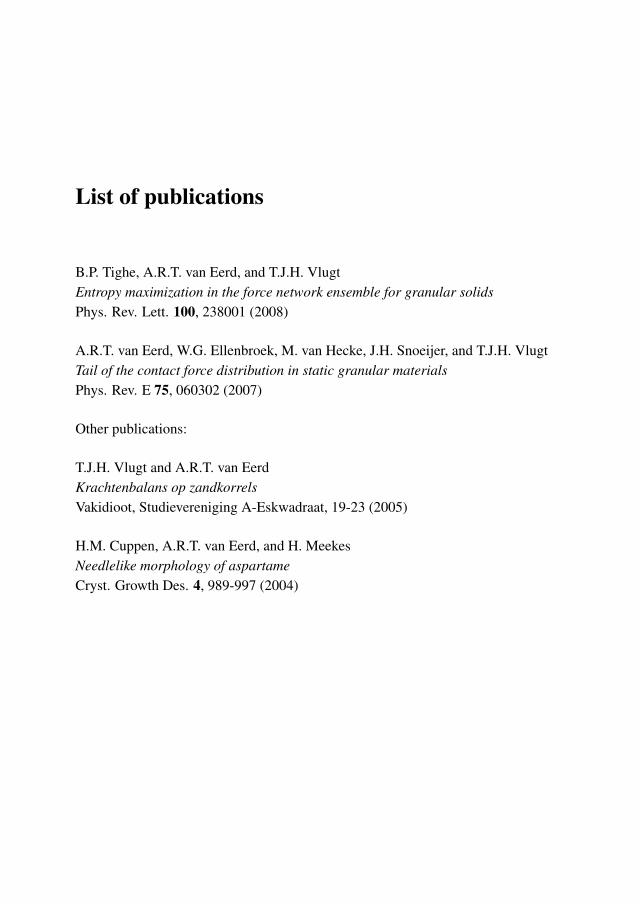
List of publications

B.P. Tighe, A.R.T. van Eerd, and T.J.H. VlugtEntropy maximization in the force network ensemble for granular solidsPhys. Rev. Lett. 100, 238001 (2008)

A.R.T. van Eerd, W.G. Ellenbroek, M. van Hecke, J.H. Snoeijer, and T.J.H. VlugtTail of the contact force distribution in static granular materialsPhys. Rev. E 75, 060302 (2007)

Other publications:

T.J.H. Vlugt and A.R.T. van EerdKrachtenbalans op zandkorrelsVakidioot, Studievereniging A-Eskwadraat, 19-23 (2005)

H.M. Cuppen, A.R.T. van Eerd, and H. MeekesNeedlelike morphology of aspartameCryst. Growth Des. 4, 989-997 (2004)

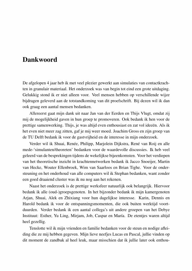
Dankwoord

De afgelopen 4 jaar heb ik met veel plezier gewerkt aan simulaties van contactkrach-ten in granulair materiaal. Het onderzoek was van begin tot eind een grote uitdaging.Gelukkig stond ik er niet alleen voor. Veel mensen hebben op verschillende wijzebijdragen geleverd aan de totstandkoming van dit proefschrift. Bij dezen wil ik danook graag een aantal mensen bedanken.

Allereerst gaat mijn dank uit naar Jan van der Eerden en Thijs Vlugt, omdat zijmij de mogelijkheid gaven in hun groep te promoveren. Ook bedank ik hen voor deprettige samenwerking. Thijs, je was altijd even enthousiast en zat vol ideeën. Als ikhet even niet meer zag zitten, gaf je mij weer moed. Joachim Gross en zijn groep vande TU Delft bedank ik voor de gastvrijheid en de interesse in mijn onderzoek.

Verder wil ik Shuai, Renée, Philipp, Marjolein Dijkstra, René van Roij en allemede-‘simulanten/theoreten’ bedanken voor de waardevolle discussies. Ik heb veelgeleerd van de besprekingen tijdens de wekelijkse bijeenkomsten. Voor het verdiepenvan het theoretische inzicht in krachtennetwerken bedank ik Jacco Snoeijer, Martinvan Hecke, Wouter Ellenbroek, Wim van Saarloos en Brian Tighe. Voor de onder-steuning en het onderhoud van alle computers wil ik Stephan bedanken, want zondereen goed draaiend cluster was ik nu nog aan het rekenen.

Naast het onderzoek is de prettige werksfeer natuurlijk ook belangrijk. Hiervoorbedank ik alle (oud-)groepsgenoten. In het bijzonder bedank ik mijn kamergenotenArjan, Shuai, Alek en Zhixiang voor hun dagelijkse interesse. Karin, Dennis enHarold bedank ik voor de ontspanningsmomenten, die ook buiten werktijd voort-duurden. Verder bedank ik een aantal collega’s uit andere groepen van het DebyeInstituut: Esther, Yu Ling, Mirjam, Job, Caspar en María. De etentjes waren altijdheel gezellig.

Tenslotte wil ik mijn vrienden en familie bedanken voor de steun en nodige aflei-ding die ze mij hebben gegeven. Mijn lieve neefjes Lucas en Pascal, jullie vinden opdit moment de zandbak al heel leuk, maar misschien dat ik jullie later ook enthou-

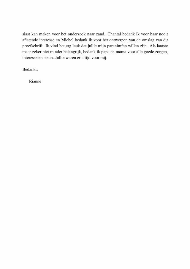
siast kan maken voor het onderzoek naar zand. Chantal bedank ik voor haar nooitaflatende interesse en Michel bedank ik voor het ontwerpen van de omslag van ditproefschrift. Ik vind het erg leuk dat jullie mijn paranimfen willen zijn. Als laatstemaar zeker niet minder belangrijk, bedank ik papa en mama voor alle goede zorgen,interesse en steun. Jullie waren er altijd voor mij.

Bedankt,

Rianne