Status report of

WG2 - Numerics and Dynamics

COSMO General Meeting05.-09.09.2010, Moscow

Michael BaldaufDeutscher Wetterdienst, Offenbach, Germany

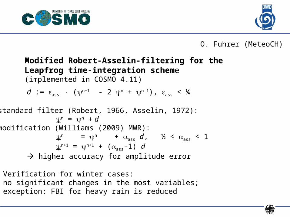
O. Fuhrer (MeteoCH)

Modified Robert-Asselin-filtering for the Leapfrog time-integration scheme(implemented in COSMO 4.11)

d := ass (n+1 - 2 n + n-1), ass < ¼

standard filter (Robert, 1966, Asselin, 1972): n = n + d

modification (Williams (2009) MWR): n = n + ass d, ½ < ass < 1 n+1 = n+1 + (ass-1) d

higher accuracy for amplitude error

Verification for winter cases:no significant changes in the most variables;exception: FBI for heavy rain is reduced

Potential temperature advection with tendency limiter

With potential temperature as advected variable, the adiabatic heating term and advection of the basic state temperature gradient disappear

Allows for limiting tendencies of quasi-horizontal advection (i.e. along terrain-following coordinate surfaces) without corrections for adiabatic heating/cooling

Present implementation: advection must not intensify local extrema exceeding the average of the neighbouring grid points by 2.5 K

The 2.5 K threshold was empirically determined by requesting negligible impact on cold-air advection along marginally resolved valleys

G. Zängl (DWD)

Potential temperature advection with tendency limiter

Since October 2009, potential temperature advection is operationally used at MeteoSwiss for COSMO-2

Afterwards, no runaway cold pools (which sometimes even led to crashes) occurred any more

Verification results indicate notable reduction of wintertime cold bias in Alpine valleys even in cases without runaway cold pools

Positive side impact on wintertime dew point temperature, cloud cover, and precipitation frequency bias in Alpine valleys, small effects otherwise

Small and indifferent impact in summer

G. Zängl (DWD)

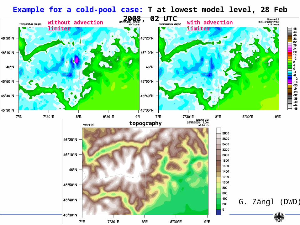
Example for a cold-pool case: T at lowest model level, 28 Feb 2008, 02 UTC

without advection limiter with advection limiter

topography

G. Zängl (DWD)

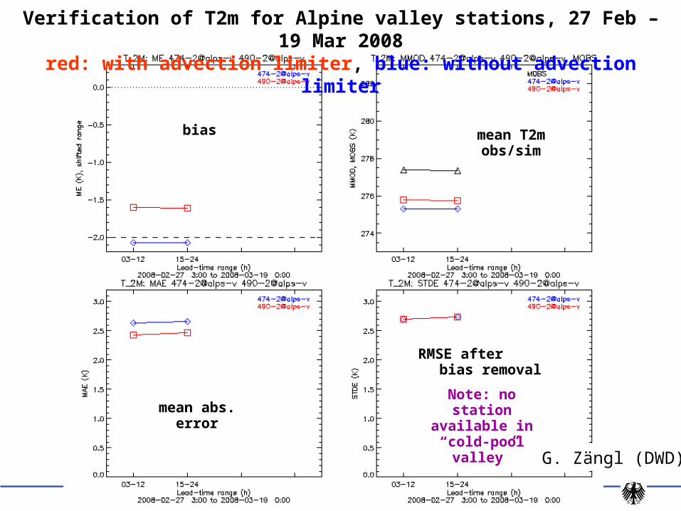
bias

mean abs. error

Verification of T2m for Alpine valley stations, 27 Feb – 19 Mar 2008red: with advection limiter, blue: without advection limiter

mean T2m obs/sim

RMSE after bias removal

Note: no station available in “cold-

pool valley”

G. Zängl (DWD)

FE 13 – 19.04.23

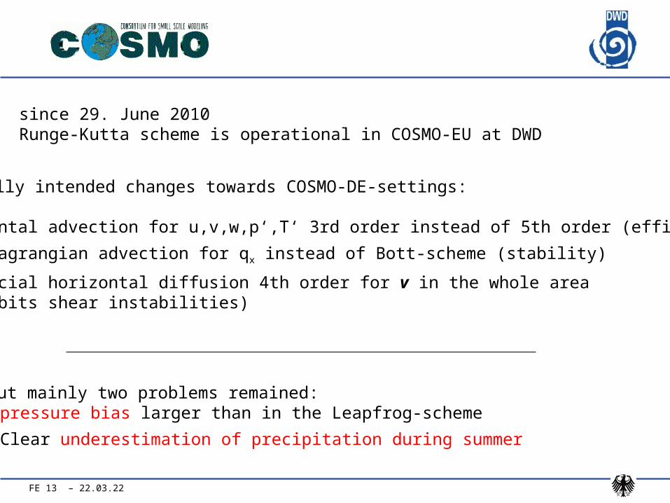
originally intended changes towards COSMO-DE-settings:

• horizontal advection for u,v,w,p‘,T‘ 3rd order instead of 5th order (efficiency)

• Semi-Lagrangian advection for qx instead of Bott-scheme (stability)

• artificial horizontal diffusion 4th order for v in the whole area (prohibits shear instabilities)

But mainly two problems remained:• pressure bias larger than in the Leapfrog-scheme

• Clear underestimation of precipitation during summer

since 29. June 2010Runge-Kutta scheme is operational in COSMO-EU at DWD

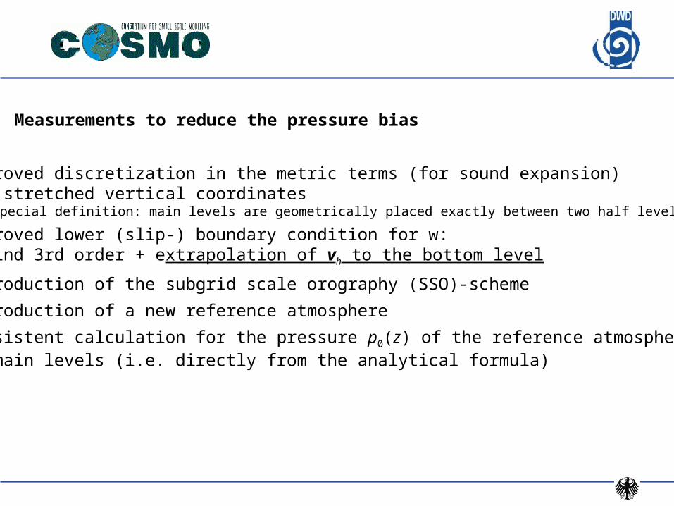
Measurements to reduce the pressure bias

• improved discretization in the metric terms (for sound expansion)for stretched vertical coordinates( special definition: main levels are geometrically placed exactly between two half levels)

• improved lower (slip-) boundary condition for w: upwind 3rd order + extrapolation of vh to the bottom level

• introduction of the subgrid scale orography (SSO)-scheme

• introduction of a new reference atmosphere

• consistent calculation for the pressure p0(z) of the reference atmosphere on main levels (i.e. directly from the analytical formula)

Bug fix for combination Tiedtke scheme – RK core

What was wrong?

In version 4.4, a temperature-dependent partitioning of detrained water substance between cloud water and cloud ice was introduced

The cloud ice tendency was correctly processed in the LF core but was written to an afterwards unused variable in the RK core

Effect: substantial loss of moisture in summer

G. Zängl (DWD)

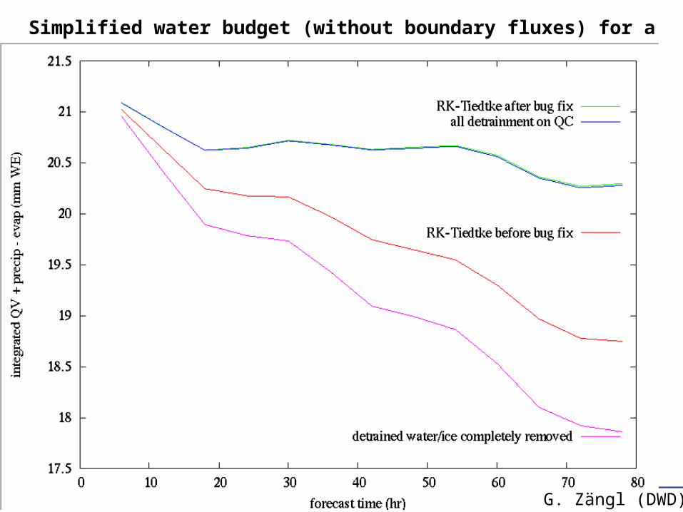
Simplified water budget (without boundary fluxes) for a COSMO-EU test

G. Zängl (DWD)

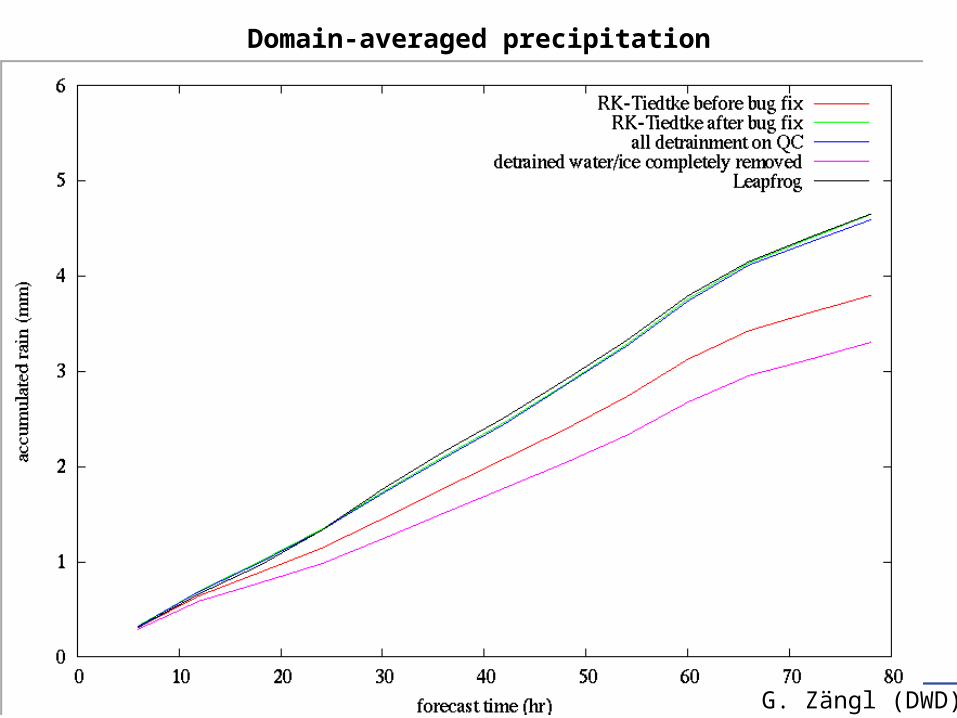
Domain-averaged precipitation

G. Zängl (DWD)

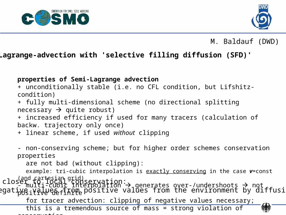
Semi-Lagrange-advection with 'selective filling diffusion (SFD)'

M. Baldauf (DWD)

to get closer to local conservation:fill negative values from positive values from the environment by diffusion

properties of Semi-Lagrange advection+ unconditionally stable (i.e. no CFL condition, but Lifshitz-condition) + fully multi-dimensional scheme (no directional splitting necessary quite robust)+ increased efficiency if used for many tracers (calculation of backw. trajectory only once)+ linear scheme, if used without clipping

- non-conserving scheme; but for higher order schemes conservation properties are not bad (without clipping):example: tri-cubic interpolation is exactly conserving in the case v=const (and cartesian grid)

- multi-cubic interpolation generates over-/undershoots not positive definitefor tracer advection: clipping of negative values necessary; this is a tremendous source of mass = strong violation of conservation

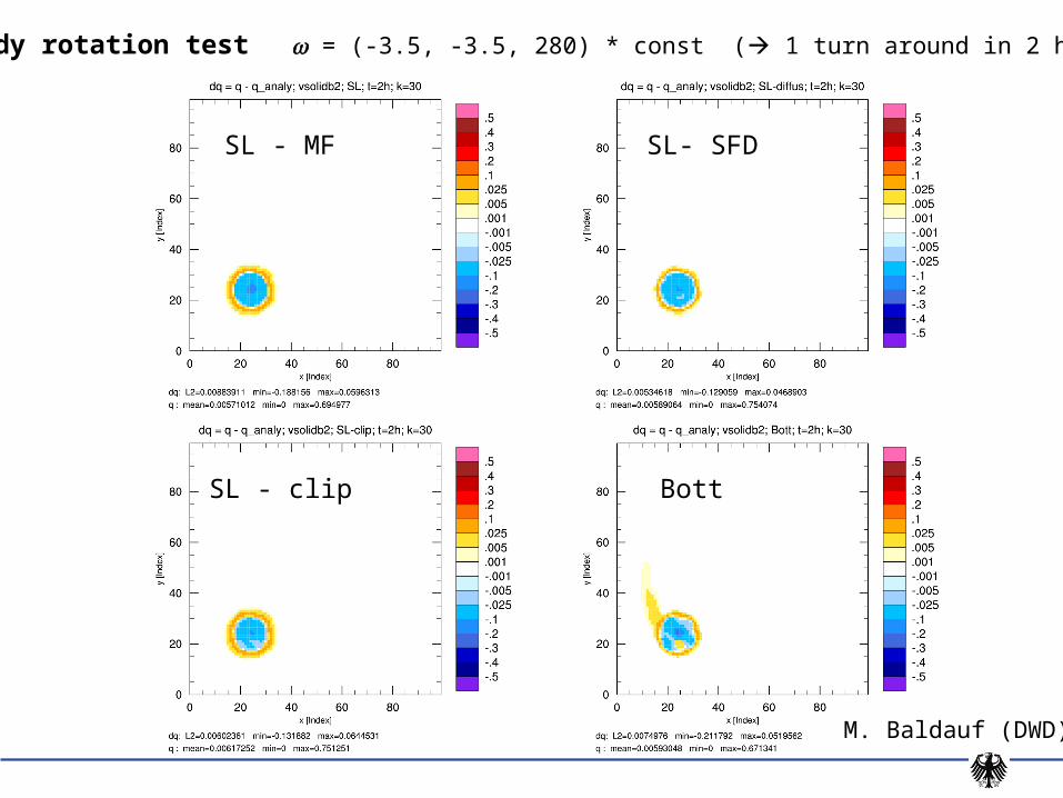
Solid body rotation test = (-3.5, -3.5, 280) * const ( 1 turn around in 2 h)

SL - MF SL- SFD

SL - clip Bott

M. Baldauf (DWD)

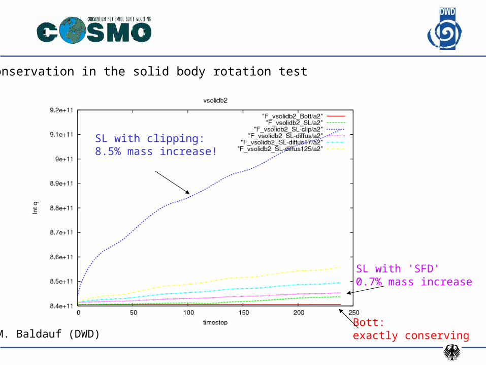
SL with clipping:8.5% mass increase!

Bott: exactly conserving

SL with 'SFD'0.7% mass increase

Conservation in the solid body rotation test

M. Baldauf (DWD)

PBPV – 03/2010

Summary

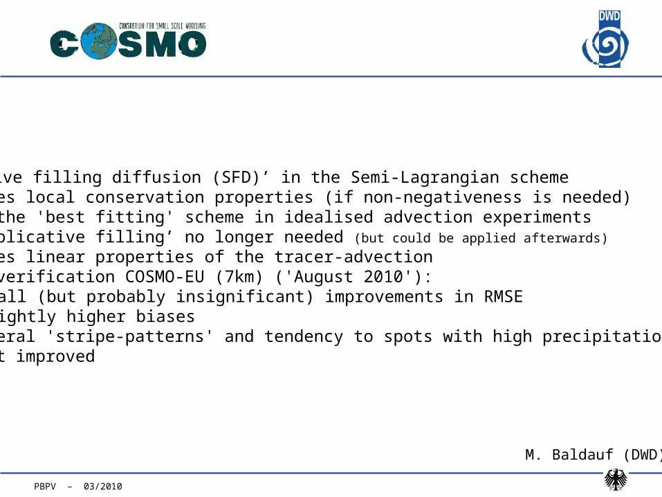
‘selective filling diffusion (SFD)’ in the Semi-Lagrangian scheme• improves local conservation properties (if non-negativeness is needed)• often the 'best fitting' scheme in idealised advection experiments• ‘multiplicative filling’ no longer needed (but could be applied afterwards)

• improves linear properties of the tracer-advection• synop-verification COSMO-EU (7km) ('August 2010'):

• small (but probably insignificant) improvements in RMSE• slightly higher biases

• in general 'stripe-patterns' and tendency to spots with high precipitation hasnot yet improved

M. Baldauf (DWD)

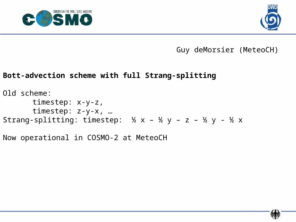
Bott-advection scheme with full Strang-splitting

Old scheme: timestep: x-y-z,timestep: z-y-x, …

Strang-splitting: timestep: ½ x – ½ y – z – ½ y - ½ x

Now operational in COSMO-2 at MeteoCH

Guy deMorsier (MeteoCH)

DFG-Priority Program ‘Metström’2nd program phase (=years 3+4)Project ‘Adaptive numerics for multi-scale flow’ will be further maintained

Since 01.09.2010 PhD-position is staffed at DWD

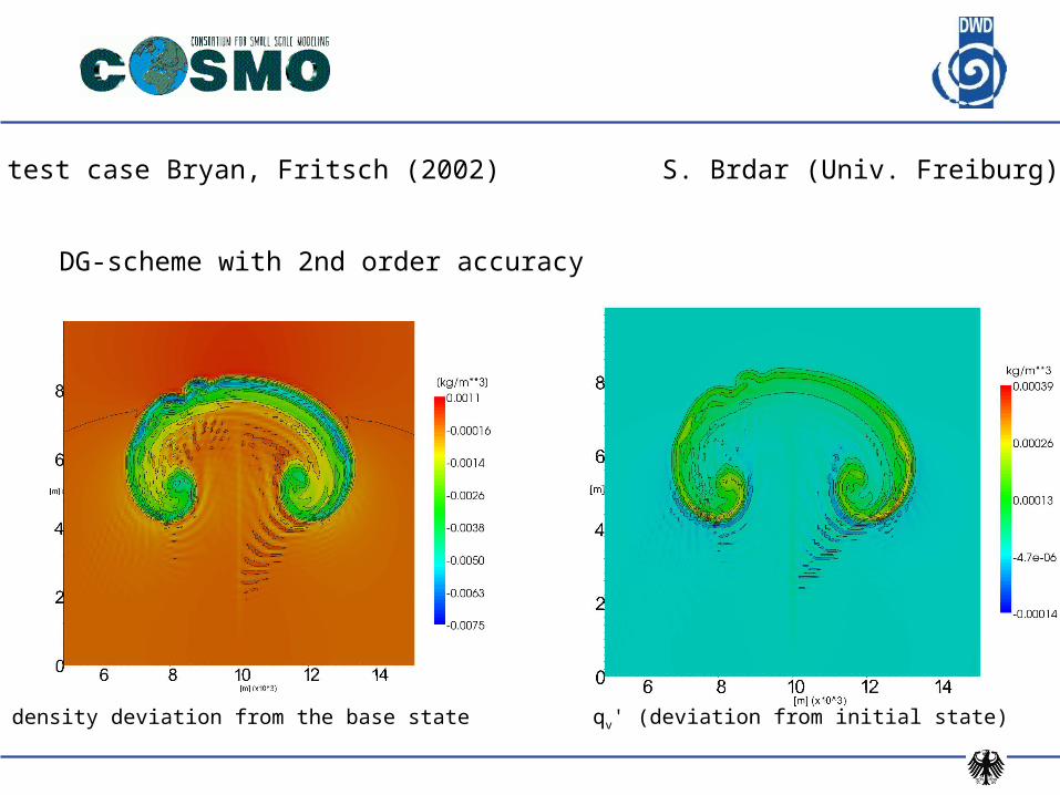
density deviation from the base state qv' (deviation from initial state)

test case Bryan, Fritsch (2002)

DG-scheme with 2nd order accuracy

S. Brdar (Univ. Freiburg)

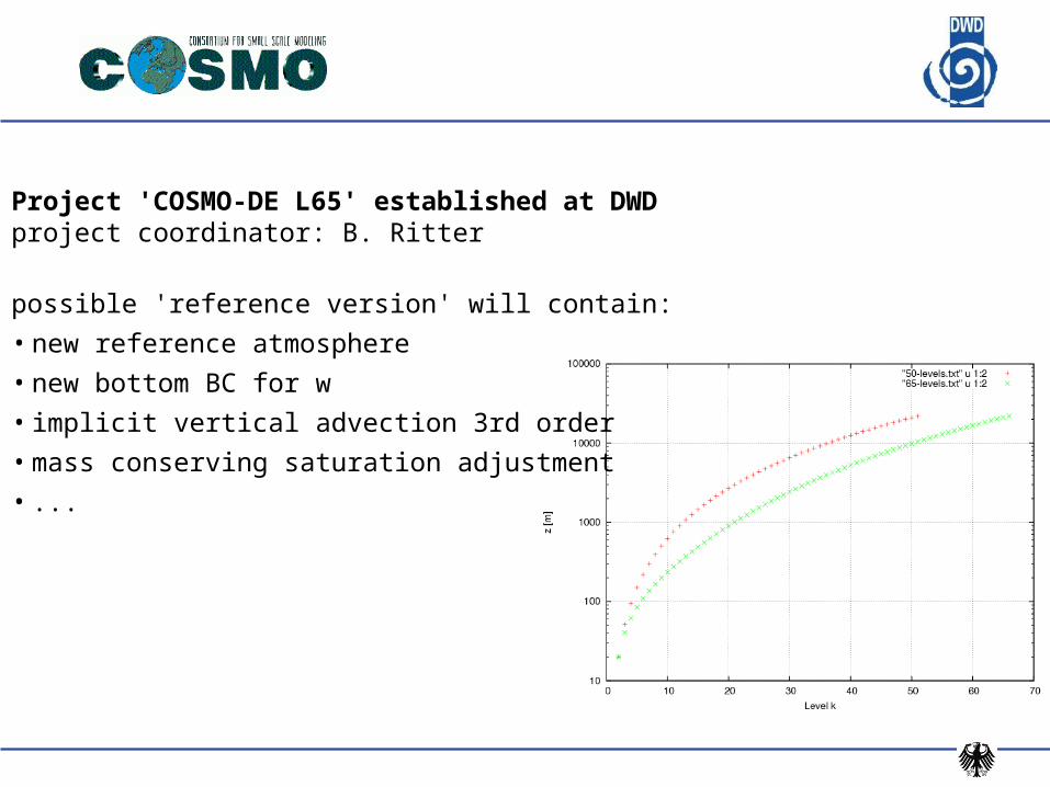
Project 'COSMO-DE L65' established at DWDproject coordinator: B. Ritter

possible 'reference version' will contain:

• new reference atmosphere

• new bottom BC for w

• implicit vertical advection 3rd order

• mass conserving saturation adjustment

• ...

WG2-publications in 2009/2010

Reviewed papers:

• M. Baldauf (2010): Linear stability analysis of Runge-Kutta based time-splitting schemes for the Euler equations, accepted by Mon. Wea. Rev.,DOI 10.1175/2010MWR3355.1

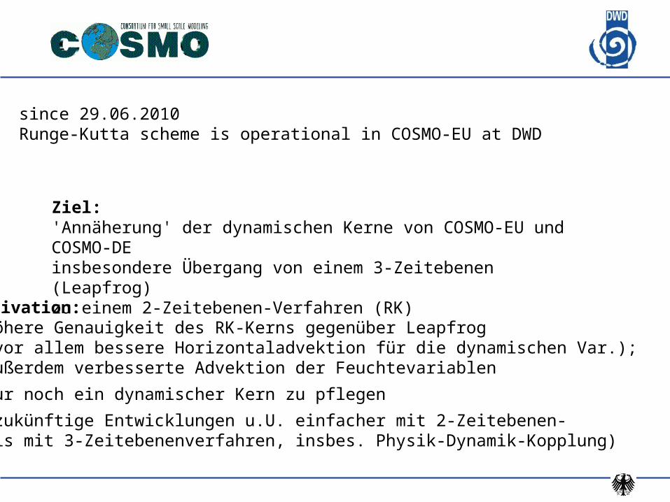
Ziel:'Annäherung' der dynamischen Kerne von COSMO-EU und COSMO-DEinsbesondere Übergang von einem 3-Zeitebenen (Leapfrog) zu einem 2-Zeitebenen-Verfahren (RK)

Motivation:• höhere Genauigkeit des RK-Kerns gegenüber Leapfrog

(vor allem bessere Horizontaladvektion für die dynamischen Var.);außerdem verbesserte Advektion der Feuchtevariablen

• nur noch ein dynamischer Kern zu pflegen

• (zukünftige Entwicklungen u.U. einfacher mit 2-Zeitebenen- als mit 3-Zeitebenenverfahren, insbes. Physik-Dynamik-Kopplung)

since 29.06.2010Runge-Kutta scheme is operational in COSMO-EU at DWD

H

zTTzT exp)( 000

Einführung einer neuen Referenzatmosphäre:

Vorteile:• realistischere Temperaturen in der Stratosphäre• keine Beschränkung für die Lage des Modelloberrandes

(in der alten Ref.-atm. gilt T< 0 K für z > ~30 km)

(Anm.: die hydrostatische Gl. läßt sich damit analytisch integrieren p0(z) = ... )

Eine Referenzatmosphäre reduziert insbesondere numerische Fehlerbei der Berechnung des Druckgradienten in geländefolgenden Koordinaten

Zerlege: p = p0+ p', T=T0+T '