Stochastic characterization of upstream demand processes in a supply chain

This article was downloaded by: [Case Western Reserve University]On: 23 November 2014, At: 04:55Publisher: Taylor & FrancisInforma Ltd Registered in England and Wales Registered Number: 1072954 Registered office: Mortimer House,37-41 Mortimer Street, London W1T 3JH, UK

IIE TransactionsPublication details, including instructions for authors and subscription information:http://www.tandfonline.com/loi/uiie20

Stochastic characterization of upstream demandprocesses in a supply chainLAYTH C. ALWAN a , JOHN J. LIU a & DONG-QING YAO ba School of Business Administration, University of Wisconsin-Milwaukee, PO Box 742,Milwaukee, WI 53201, USA E-mail: [email protected] or [email protected] College of Business and Economics, Towson University, Towson, MD 21252, USA E-mail:[email protected] online: 29 Oct 2010.

To cite this article: LAYTH C. ALWAN , JOHN J. LIU & DONG-QING YAO (2003) Stochastic characterization of upstream demandprocesses in a supply chain, IIE Transactions, 35:3, 207-219, DOI: 10.1080/07408170304368

To link to this article: http://dx.doi.org/10.1080/07408170304368

PLEASE SCROLL DOWN FOR ARTICLE

Taylor & Francis makes every effort to ensure the accuracy of all the information (the “Content”) containedin the publications on our platform. However, Taylor & Francis, our agents, and our licensors make norepresentations or warranties whatsoever as to the accuracy, completeness, or suitability for any purpose of theContent. Any opinions and views expressed in this publication are the opinions and views of the authors, andare not the views of or endorsed by Taylor & Francis. The accuracy of the Content should not be relied upon andshould be independently verified with primary sources of information. Taylor and Francis shall not be liable forany losses, actions, claims, proceedings, demands, costs, expenses, damages, and other liabilities whatsoeveror howsoever caused arising directly or indirectly in connection with, in relation to or arising out of the use ofthe Content.

This article may be used for research, teaching, and private study purposes. Any substantial or systematicreproduction, redistribution, reselling, loan, sub-licensing, systematic supply, or distribution in anyform to anyone is expressly forbidden. Terms & Conditions of access and use can be found at http://www.tandfonline.com/page/terms-and-conditions

http://www.tandfonline.com/loi/uiie20

http://www.tandfonline.com/action/showCitFormats?doi=10.1080/07408170304368

http://dx.doi.org/10.1080/07408170304368

http://www.tandfonline.com/page/terms-and-conditions

http://www.tandfonline.com/page/terms-and-conditions

Stochastic characterization of upstream demand processes ina supply chain

LAYTH C. ALWAN1, JOHN J. LIU1 and DONG-QING YAO2

1School of Business Administration, University of Wisconsin-Milwaukee, PO Box 742, Milwaukee, WI 53201, USAE-mail: [email protected] or [email protected] of Business and Economics, Towson University, Towson, MD 21252, USAE-mail: [email protected]

Received September 2000 and accepted September 2001

In the supply chain management area, there has much recent attention to a phenomenon known as the bullwhip effect. Thebullwhip effect represents the situation where demand variability increases as one moves up the supply chain. In this paper, westudy this effect in an order-up-to supply-chain system when minimum Mean Square Error (MSE) optimal forecasting is employedas opposed to some commonly used simplistic forecasting schemes. We find that depending on the correlative structure of thedemand process it is possible to reduce, or even eliminate (i.e., ‘‘de-whip’’), the bullwhip effect in such a system by using an MSE-optimal forecasting scheme. Beyond the bullwhip effect, we also determine the exact time-series nature of the upstream demandprocesses.

1. Introduction

One important supply chain research problem that hasdrawn much attention is the phenomenon known as thebullwhip effect. The bullwhip effect represents the situa-tion where demand variability amplifies as one moves upthe supply chain. In a single-item two-stage supply chain,it means, in particular, that the variability of the ordersreceived by the supplier is greater than the demandvariability observed by the buyer.It has been recognized that demand forecasting and

ordering policies are among two of the key causes of thebullwhip effect (e.g., Lee et al., 1997). The connectionbetween forecasting and the bullwhip effect is surmisedfrom the fact that an order for supply placed at any giventime attempts to meet projected demand. As such, therehave been an increasing number of studies devoted to thestudy of the magnitude of the bullwhip effect given somestochastic demand pattern, a forecasting method, and anordering policy (e.g., Graves, 1999; Chen et al., 2000a,2000b). The findings from these studies all indicate thatthe bullwhip effect is indeed present under differentforecasting methods and different demand patterns.Furthermore, all the studies to date have shown that thebullwhip effect increases without limit as the lead-timeincreases.It is important to mention that Graves (1999) studied

the bullwhip effect resulting from a myopic base-stock

policy in conjunction with the use of an optimal fore-casting scheme for a particular nonstationary demandprocess, namely, a first-order integrated moving-averageprocess or ARIMA(0,1,1) process, whereas Chen et al.(2000a, 2000b) studied the bullwhip effect resulting froman order-up-to policy when two common, but simplified,forecasting schemes – the moving-average method andthe Exponential Weighted Moving-Average (EWMA)method – are used for a particular stationary demandprocess, namely, a first-order autoregressive process orAR(1) process. However, as the authors of the order-up-to policy study pointed out themselves, one limitation oftheir study is that they ‘‘are not using the optimal fore-casting technique for the correlated demand processconsidered here’’ (Chen et al., 2000a, p. 442).This paper provides three distinct contributions. First,

for an AR(1) demand process and an order-up-to policy,we study the bullwhip effect when an optimal forecastingscheme is used, as opposed to consideration of only non-optimal schemes such as the moving-average andEWMA. In the area of forecasting, an ‘‘optimal’’ fore-casting model is traditionally meant to imply that theforecasting model has minimum mean square forecasterrors. For clarity, we will refer to such a model as aMean Square Error-optimal (or MSE-optimal) forecast-ing model. When investigating the bullwhip effect, thevariance of the ordering random variable is only derived.Our second contribution is to fully characterize ordering

0740-817X � 2003 ‘‘IIE’’

IIE Transactions (2003) 35, 207–219

Copyright� 2003 ‘‘IIE’’

0740-817X/03 $12.00+.00

DOI: 10.1080/07408170390175440

Dow

nloa

ded

by [

Cas

e W

este

rn R

eser

ve U

nive

rsity

] at

04:

55 2

3 N

ovem

ber

2014

random variable beyond the variance parameter. Inparticular, we determine the underlying time-series modelfor the ordering process. It should be pointed out thatGraves (1999) made a similar contribution in terms ofcharacterizing the ordering process resulting from a base-stock policy when an EWMA forecasting scheme wasapplied to an ARIMA(0,1,1) process.We will also be able to provide insights on the ordering

process when the demand process follows another com-mon stationary process, namely, a mixed first-orderautoregressive/first-order moving-average process orARMA(1,1). Finally, our study of the ARMA(1,1) willenable us to make certain generalizations for a multiple-stage supply chain.The remainder of this paper is organized as follows.

Section 2 introduces the AR(1) demand process andpresents an order-up-to policy. Section 3 compares thebullwhip effect under the MSE-optimal forecastingmethod versus the moving-average method and EWMAmethod. In addition, for each of the three noted fore-casting schemes, Section 3 presents the stochastic natureof the ordering process. Section 4 considers the stochasticnature of the upstream demand process for an incomingARMA(1,1) demand process when an MSE-optimalforecasting scheme is used. Section 5 offers our conclud-ing remarks.

2. A single-item supply chain under AR(1) demand

As noted, we are considering a single-item two-stagesupply chain. The lead-time (L) is fixed and known.There are a number of potential stochastic processesthat can be assumed for the demand process, rangingfrom a simple independent and identically distributed(iid) process to a nonstationary process. In reality, thereis empirical evidence that few real-world (demand orotherwise) processes exhibit pure iid behavior (Alwan,2000). One flexible correlative demand process that hasbeen studied in the supply chain literature is the AR(1)model (Kahn, 1987; Lee et al., 1997, 2000; Chen et al.2000a, 2000b). In the following subsections, we describethe AR(1) model in more detail, present the forecastingmodels to be considered, and present the orderingpolicy to be examined in this paper.

2.1. Demand process

Suppose the system is faced with an AR(1) demandprocess given as follows:

dt ¼ sþ /dt�1 þ et t ¼ 0;�1;�2; . . . ð1Þwhere dt is the observed demand for period t, s > 0,/j j < 1, and etf g is an independent and identically dis-tributed normal (iidn) process with mean zero and vari-ance r2e . The condition of /j j < 1 ensures that the process

is stationary. It is useful to note that ld ¼ EðdtÞ ¼s=ð1� /Þ and r2d ¼ VarðdtÞ ¼ r2e ð1� /2Þ�

for any t.By varying the values of /, one can represent a wide

variety of process behaviors. When / ¼ 0, we have aniidn process with mean s and variance r2e . For�1 < / < 0, the process is negatively correlated and willexhibit period-to-period oscillatory behavior. For0 < / < 1, the demand process will be positively corre-lated which is reflected by a wandering or meanderingsequence of observations. As /j j approaches one, theprocess approaches nonstationary behavior; in particular,a pure random walk model or equivalently, an AR-IMA(0,1,0) process. As pointed out by Graves and Wil-lems (2000), varying a stationary demand model, such asan AR(1) model, is an important exercise for gainingfundamental insights about the relationships betweenvariables such as inventory and orders relative to a widevariety of demand characterizations.

2.2. Forecasting models

Smoothing methods, such as moving averages and ex-ponential smoothing, are widely employed for forecastingpurposes in many production and operations manage-ment applications, largely because of their simplicity andease of implementation. As such, most researchers ofSupply Chain Management (SCM) problems requiring aforecasting model have based their studies on either themoving-average method or the EWMA method (e.g.,Chen et al., 2000a, 2000b).The moving-average forecasting model of length p can

be expressed as follows:

Ftþ1 ¼Pp�1

i¼0 dt�i

p; ð2Þ

where Ftþ1 is the forecast of period t þ 1 made at the endof period t. It should be noted that the forecasts for pe-riods t þ i (i ¼ 1; 2; . . .) made at time t are equal, that is,Ftþi ¼ Ftþ1 for i ¼ 1,2, . . . Hence, the forecasts for all leadtimes will follow a horizontal line parallel to the time axis.The EWMA model can be expressed as follows:

Ftþ1 ¼ adt þ ð1� aÞFt; ð3Þwhere 0 < a � 1 is the smoothing constant. Similar to themoving-average technique, forecasts for periods t þ i(i ¼ 1; 2; . . .) made at time t are equal.Even though the EWMAmethod, and to a lesser extent

the moving-average method, has flexibility for adaptingto a variety of correlated demand processes, it is MSE-optimal for only one underlying time-series model,namely, an ARIMA(0,1,1) process with no constant term(Hamilton, 1994). In general, an ARIMA(0,1,1) processis a nonstationary process that can be interpreted as arandom-walk trend plus a random deviation from thetrend. Thus, under no circumstance is the EWMA

208 Alwan et al.

Dow

nloa

ded

by [

Cas

e W

este

rn R

eser

ve U

nive

rsity

] at

04:

55 2

3 N

ovem

ber

2014

method MSE-optimal for a stationary AR(1) process.This fact opens up consideration of employing an MSE-optimal forecasting scheme for the assumed AR(1) pro-cess.By recursively applying (1), it is easy to show that:

dtþi ¼ sþ /sþ � � � þ /i�1sþ /idt þ /i�1etþ1 þ /i�2etþ2

þ � � � þ etþi ¼ 1� /i

1� /sþ /idt þ /i�1etþ1

þ /i�2etþ2 þ � � � þ etþi: ð4ÞFor a general ARIMA process, it can be shown that theminimum MSE forecast for period t þ i is the conditionalexpectation of dtþi given current and previous observa-tions dt,dt�1,dt�2 , . . . (Box et al., 1994). In the case of anAR(1) process, this implies the MSE-optimal forecastfunction is given by EðdtþijdtÞ. Since EðetþijdtÞ ¼ 0 fori ¼ 1,2,. . ., it immediately follows that for an AR(1)process, the MSE-optimal forecast function is given by:

Ftþi ¼ 1� /i

1� /sþ /idt for i ¼ 1; 2; . . . ð5Þ

In contrast to the two previous methods, this forecastfunction is not a horizontal projection into the future.Instead the forecasts revert back towards the overall meanlevel of s 1� /= . The MSE-optimal forecast function re-flects the fact that the AR(1) process is stationary and hasthe property of conditional mean reversion; that is, eventhough the process can be expected to wander away (be-low or above) from the overall mean it is also expected toeventually return back to the overall mean. The moving-average and EWMA methods fail to capture this meanreversion property of a stationary AR(1) process.One argument often presented against the use of opti-

mal methods is that their implementation is more difficultthan the simple smoothing methods when parameters areunknown. It is pointed out that to implement optimalmethods requires statistical skills in time-series modeling,including knowledge of model identification, model esti-mation, and tests for model adequacy, that are beyondthe skill set of a typical operations manager. However, webelieve that the industrial use of more sophisticated time-series models is steadily growing because of two reasons.First, the requirement of intense statistical training, oftenreferred to as 6r training, is increasingly becoming com-monplace (Hoerl, 1998). At corporations like GE,Motorola, and Allied Signal, organizational cultures arebeing developed in which there is a strong desire fromemployees throughout the organization to learn and im-plement advanced statistical techniques. Indeed, the au-thors of this paper can report that seminars in time-seriesanalysis are part of the regular continuing educationprogram at GE-Medical Systems and are encouraged tobe taken by all supply chain managers. Second, moderncomputational tools are readily available to make possi-

ble automated implementation of time-series modelingincluding the general class of ARIMA models. Theseprograms are designed to automate model identification,model fitting, and forecasting (Shumway, 1986).

2.3. The order-up-to policy

We now consider the order quantity qt which is defined asthe quantity ordered at the end of period t by the buyerfor arrival from the supplier at the end of period t þ L. Aspracticed at manufacturing companies experienced by theauthors, the manufacturing lead-time L (including sup-plier’s response time) is used as the target delivery time.Thus, the production orders, and therefore the orders tothe suppliers, are based on the demand cumulated over Lperiods. For other manufacturing situations where L isdefined as manufacturing lead-time plus one period ofreview, all our subsequent results can simply be modifiedby replacing L with (Lþ 1).It should be recognized that the buyer’s order quanti-

ties could be viewed as the demand process for the sup-plier. Depending on the nature of the product andmanufacturing practices, there is a potential for a numberof different order policies. In the SCM literature, one ofthe most studied order policies is a simple order-up-topolicy, as introduced by Lee et al. (1997) and thenadopted and modified by others (e.g., Chen et al., 2000a,2000b). As opposed to an (s; S) ordering policy, it shouldbe pointed out that the order-up-to policy that will bestudied here and was initially studied by the above-notedauthors is not what might be classically interpreted in theoperations area as an order-up-to type of policy. Not-withstanding this fact, variants of such an ordering policyare reported to have many important applications in-cluding make-to-stock production (e.g., textile and ap-parel industries) where an inventory stock level isestablished by a single order in advance to cover demandsover multiple periods.The order-up-to level, denoted by yt, can be defined as

follows:

yt ¼ DDLt þ z rLe ; ð6Þ

where DDLt represents a forecast of the total expected de-

mand over L periods after period t, z is a constant term,and rLe represents the standard deviation of the L-periodforecast error. In the case when rLe is unknown, r

Le is

replaced with an appropriately chosen estimator. InSection 3.2, we will address in more detail the issue ofparameter estimation.In terms of earlier notation, we recognize that DDL

t isgiven by

PLi¼1 Ftþi. Given the earlier noted fact that both

moving-average and EWMA forecasting schemes areassociated with a horizontal forecast function, DDL

t underthese schemes is given as follows:

DDLt ¼ LFtþ1: ð7Þ

Upstream demand processes in a supply chain 209

Dow

nloa

ded

by [

Cas

e W

este

rn R

eser

ve U

nive

rsity

] at

04:

55 2

3 N

ovem

ber

2014

Using (5), we find for the MSE-optimal forecastingscheme, DDL

t is given by

DDLt ¼

XLi¼1

1� /i

1� /sþ /idt

� �;

¼ Lð1� /Þ � /ð1� /LÞð1� /Þ2 sþ /ð1� /LÞ

ð1� /Þ dt;

¼ K1ð/; s; LÞ þ /ð1� /LÞð1� /Þ dt: ð8Þ

Based on the defined order-up-to level of (6), the order-up-to policy is defined as:

qt ¼ yt � yt�1 þ dt: ð9ÞThis policy allows qt to be negative. In such a case, weassume with such an ordering policy, like Kahn (1987),Lee et al. (1997), Chen et al. 2000a, 2000b), that excessinventory can be returned without a cost penalty.

3. Order process under stationary AR(1) demand

In this section, we first determine the variance of theorder process (i.e., upstream demand process) which, inturn, will allow us to study the bullwhip phenomenonunder an MSE-optimal forecasting scheme as it compareswith the bullwhip results for the moving-average andEWMA forecasting schemes. We then derive the generalstochastic models for the ordering process qt for each ofthe three forecasting schemes considered in this paper.

3.1. Bullwhip effect

The bullwhip effect represents the phenomenon whereinformation about demand becomes increasingly dis-torted as it moves upstream in the supply chain. Such adistortion can lead to excessive inventory throughout thesupply chain system, insufficient or excessive capacities,product unavailability, and higher costs in general.To show the existence of a bullwhip effect, researchers

demonstrate for a given supply chain scenario that thevariance of the order, or upstream demand, process isgreater than the variance of the demand process, that is,VarðqtÞ > VarðdtÞ or, equivalently, VarðqtÞ=VarðdtÞ > 1.When using an order-up-to policy (9) in the presence ofAR(1) demand behavior with the moving-average fore-casting method, it can be shown that:

VarðqtÞVarðdtÞ ¼ 1þ

2Lpþ 2L

2

p2

� �ð1� /pÞ: ð10Þ

Under the same policy and demand process scenario,when the EWMA forecasting method is employed thefollowing result is found:

VarðqtÞVarðdtÞ ¼ 1þ 2Laþ 2L

2a2

2� a

� �1� /

1� ð1� aÞ/� �

: ð11Þ

It is interesting to note that the results of (10) and (11) arein agreement with the ones obtained under other variantsof the order-up-to policy (e.g., Chen et al., 2000a, 2000b).In particular, the right-hand-sides of (10) and (11) are thelower bounds of the variance ratios found in these notedpapers. On that note, it should be emphasized that ourstudy is not intended to be a cross-comparison with othervariants of order-up-to policies, but rather it focuses on acomparative study of optimal versus non-optimal fore-casting schemes under the specific order-up-to orderingpolicy of this paper.Define Bma and Bex as the variance ratios given in (10)

and (11), respectively. In general, Bð�Þ is defined to be thebullwhip ratio with the superscript indicating the fore-casting scheme. It is easy to verify that

limL!1

Bma ! 1;

and

limL!1

Bex ! 1:

Taking the derivatives of the bullwhip ratios in (10) and(11) with respect to L, we obtain:

@Bma

@L¼ 2 1

pþ 2L

p2

� �ð1� /pÞ; ð12Þ

@Bex

@L¼ 2a þ 4La2

2 � a

� �1� /

1 � ð1 � aÞ/� �

: ð13Þ

Since

@Bma

@L> 0 for p > 0;

and

@Bex

@L> 0 for a > 0;

both Bma and Bex are strictly increasing in L. Further-more, we find that

@2Bma

@L2¼ 4

p2ð1� /pÞ; ð14Þ

@2Bex

@L2¼ 4a2ð1� /Þ

ð2� aÞ 1� ð1� aÞ/ð Þ : ð15Þ

Since

@2Bma

@L2> 0 for p > 0;

and

@2Bex

@L2> 0 for a > 0;

210 Alwan et al.

Dow

nloa

ded

by [

Cas

e W

este

rn R

eser

ve U

nive

rsity

] at

04:

55 2

3 N

ovem

ber

2014

both Bma and Bex are strictly convex in L. The demon-stration that these functions are strictly convex will proveimportant in our comparison of the MSE-optimal fore-casting method with the moving-average and EWMAforecasting methods.Consider now an MSE-optimal forecasting scheme. By

(6), (8), and (9), we can express qt as follows:

qt ¼ DDLt � DDL

t�1� �þ z rLe � rLe

� �þ dt;

¼ /ð1� /LÞð1� /Þ dt � /ð1� /LÞ

ð1� /Þ dt�1 þ dt;

¼ /ð1� /LÞð1� /Þ þ 1

� �dt � /ð1� /LÞ

ð1� /Þ dt�1: ð16Þ

For convenience, let

k ¼ /ð1� /LÞð1� /Þ :

The variance of qt is found as follows:

VarðqtÞ ¼ ðk þ 1Þ2 VarðdtÞ þ k2 Varðdt�1Þ� 2ðk þ 1Þk Covðdt; dt�1Þ;

¼ ðk þ 1Þ2r2d þ k2r2d � 2ðk þ 1Þk/r2d :Thus, the bullwhip ratio is given by:

VarðqtÞVarðdtÞ ¼

ðk þ 1Þ2r2d þ k2r2d � 2ðk þ 1Þk/r2dr2d

;

¼ ðk þ 1Þ2 þ k2 � 2ðk þ 1Þk/: ð17ÞReplacing

k ¼ /ð1� /LÞð1� /Þ ;

into (17) and after some algebraic simplification, we find:

Bopt ¼ VarðqtÞVarðdtÞ ¼ 1þ

2/ð1� /LÞ1� /

ð1� /Lþ1Þ: ð18Þ

From (18), it follows that for �1 < / < 1,

limL!1

Bopt ¼ 1þ /1� /

: ð19Þ

Thus, in contrast to the moving-average and EWMAforecasting schemes, the bullwhip effect does not increasewithout limit as a function of lead-time but rather has alimiting value.From this point on, it will prove convenient to consider

the notation of Bð�Þþ and Bð�Þ

� which are meant to denotethe bullwhip ratio Bð�Þ when 0 < / < 1 and �1 < / � 0,respectively. For �1 < / � 0, the bullwhip ratio in (18)can be expressed as:

Bopt� ¼ 1� 2j/jð1�j/jLÞ1þj/j ð1þ j/jLþ1Þ; for L ¼ 2j ðj ¼ 1; 2; 3; . . .Þ,

1� 2j/jð1þj/jLÞ1þj/j ð1� j/jLþ1Þ; for L ¼ 2jþ 1ðj ¼ 0; 1; 2; . . .Þ.

8<:

ð20Þ

From (20), it can be easily verified that Bopt� � 1 for allL � 1. Hence, under the MSE-optimal forecasting meth-od, the bullwhip effect does not exist for negatively cor-related demand processes. Close study of (10) and (11)reveals following facts:

Bma� � Bmaþ > 1 for all L � 1; ð21ÞBex� � Bexþ > 1 for all L � 1: ð22Þ

The above conditions along with the noted fact thatBopt� � 1 for all L � 1 leads to the following proposition:

Proposition 1. For p > 0, and 0 < a � 1, it holds for allL � 1 that min½Bma� ;Bex� � > Bopt� :

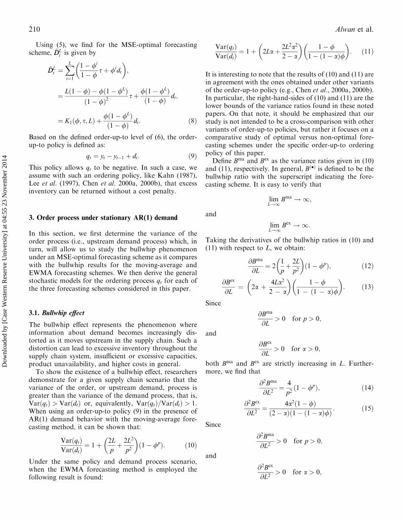
As an example, Fig. 1 shows a comparison of thebullwhip ratios for / ¼ �0:6, p ¼ 10, and a ¼ 0:1. It canbe seen quite clearly from this figure that the bullwhipeffect exists and amplifies with lead-time for the moving-average and EWMA methods. In dramatic contrast, thebullwhip effect does not exist and, in fact, for this par-ticular value of / the variance of the ordering processdiminishes with lead-time.For 0 < / < 1, we can obtain from (18) the following:

@Boptþ@L

¼ �2/Lþ1 lnð/Þ � 4 lnð/Þ1� /ð Þ/

Lþ2ð1� /LÞ;

¼ � 2/Lþ1 lnð/Þ1� /

1� /þ 2/ð1� /LÞ� : ð23Þ

Since lnð/Þ < 0 for 0 < / < 1, we can see that

@Boptþ@L

> 0 for L > 0:

As such, we can conclude that Boptþ is strictly increasing inL. For 0 < / < 1, the second derivative of the bullwhipratio is given by:

@2Boptþ@L2

¼ � 2 lnð/Þ½ �2/Lþ1

1� /1þ /� 4/Lþ1� �

: ð24Þ

Fig. 1. Bullwhip effects as a function of L with / ¼ �0:6,p ¼ 10, and a ¼ 0:1.


Dow

nloa

ded

by [

Cas

e W

este

rn R

eser

ve U

nive

rsity

] at

04:

55 2

3 N

ovem

ber

2014

This implies that the convexity of Boptþ is dependent on thesign of the last term in (24), 1þ /� 4/Lþ1� �

. The sign ofthe term can be easily determined by solving the equation:1þ /� 4/Lþ1 ¼ 0. With constraint of L � 1, solving forL the equation 1þ /� 4/Lþ1 ¼ 0 will yield the resultthat Boptþ is concave for L � LL and convex for L < LL where

LL ¼ max 1; lnð1þ /Þ=4lnð/Þ � 1

� �� :

It can also be verified that if / � 1þ ffiffiffiffiffi17

p� �=8 ¼ 0:6404

then Boptþ is concave for all lead-times L � 1.Given that the bullwhip effect under MSE-optimal

forecasting is increasing at a diminishing rate for all L � LLand that it is increasing at an accelerating rate for allL � 1 under the moving-average method or EMWAmethod, it is ensured that the bullwhip effects under themoving-average method or EMWA method will surpassthat under MSE-optimal method when lead-time L be-comes large enough. Formally, we can state the follow-ing:

Proposition 2. For p > 0 and 0 < a � 1, there exists anL� < 1 such that min½Bmaþ ;Bexþ � > Boptþ for all L > L�.Specifically, L� ¼ max½L�om; L�oe� where L�om is the lead-timeat which Boptþ ¼ Bmaþ , and L�oe is the lead-time at whichBoptþ ¼ Bexþ .

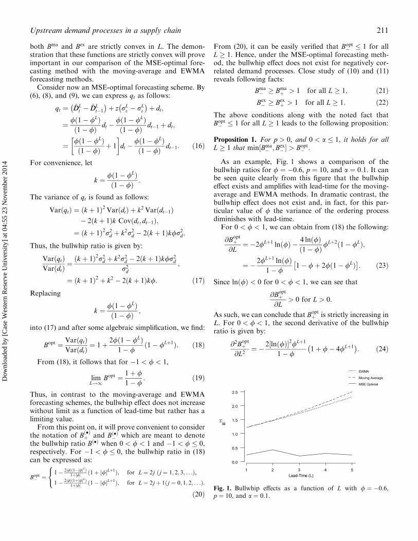
Figure 2 gives a graphical comparison of the bullwhipeffects as a function of L with / ¼ 0:6, p ¼ 6, and a ¼ 0:3.The figure confirms the convexity of Bmaþ and Bexþ alongwith the concavity of Boptþ . Most importantly, we can seefrom Fig. 2 that both bullwhip functions Bmaþ and Bexþeventually surpass Boptþ .As noted in Proposition 2, the thresholds L�om and L�oe

can be determined by setting Boptþ ¼ Bmaþ and Boptþ ¼ Bexþ ,respectively. In particular, it can be shown that for/ 2 ð0; 1Þ and p > 0, then L�om solves the following fixed-point equation:

L�om ¼ max 1; ln 1� DomðL�omÞ�

lnð/Þ Bmaþ

� �; ð25Þ

where

DomðLÞ ¼ 1� /

/ð1� /Lþ1Þ ;

and Bmaþ is given in (10) with 0 < / < 1. Similarly, for/ 2 ð0; 1Þ and 0 < a < 1, then L�oe solves the followingfixed-point equation:

L�oe ¼ max 1;ln 1� DoeðL�oeÞ� lnð/Þ Bexþ

� �; ð26Þ

where

DoeðLÞ ¼ 1� /

/ð1� /Lþ1Þ ;

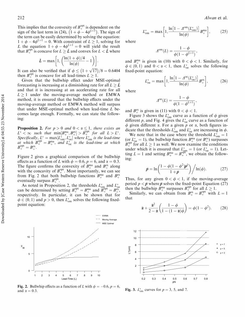
and Bexþ is given in (11) with 0 < / < 1.Figure 3 shows the L�om curve as a function of / given

different p, and Fig. 4 gives the L�oe curve as a function of/ given different a. For a given p or a, both figures in-dicate that the thresholds L�om and L�oe are increasing in /.We note that in the case where the threshold L�om ¼ 1

(or L�oe ¼ 1), the bullwhip function Bmaþ (or Bexþ ) surpassesBoptþ for all L � 1 as well. We now examine the conditionsunder which it is ensured that L�om ¼ 1 (or L�oe ¼ 1). Let-ting L ¼ 1 and setting Bmaþ ¼ Boptþ , we obtain the follow-ing:

�pp ¼ ln 1� /ð1� /2Þ�pp21þ �pp

� ��lnð/Þ: ð27Þ

Thus, for any given 0 < / < 1, if the moving-averageperiod p < �pp where �pp solves the fixed-point Equation (27)then the bullwhip Bmaþ surpasses Boptþ for all L � 1.Similarly, we can obtain from Bexþ ¼ Boptþ with L ¼ 1

that

�aaþ �aa2

2� �aa1� /

1� ð1� �aaÞ/� �

¼ /ð1� /2Þ: ð28Þ

Fig. 2. Bullwhip effects as a function of L with / ¼ �0:6, p ¼ 6,and a ¼ 0:3. Fig. 3. L�om curves for p ¼ 3, 5, and 7.

212 Alwan et al.

Dow

nloa

ded

by [

Cas

e W

este

rn R

eser

ve U

nive

rsity

] at

04:

55 2

3 N

ovem

ber

2014

Combining and re-arranging terms, we can re-write (28)as follows:

�aa3 � b�aa2 þ c�aaþ d ¼ 0; ð29Þwhere

b ¼ 2þ /ð1� /2Þ; c ¼ 2/ð1� /2Þ � ð1� /Þb/

;

d ¼ 2ð1� /2Þð1� /Þ: ð30ÞThen for any given 0 < / < 1, the bullwhip Bexþ surpassesBoptþ for all L � 1, if the smoothing constant a > �aa where�aa 2 ð0; 1� is the real root of the cubic algebra equa-tion (29), which can be determined as:

�aa ¼ffiffiffiffiffiffiffiffiffiffiffiffiffiffiffiffiffiffiffiffiffiffiffiffiffiffiffiffiffiffiffiffiffiffiffiffiffiffiffiffiffiffi� u2þ

ffiffiffiffiffiffiffiffiffiffiffiffiffiffiffiffiffiffiffiffiffiffiffiffiu2

� 2þ v3

� 3r3

sþ

ffiffiffiffiffiffiffiffiffiffiffiffiffiffiffiffiffiffiffiffiffiffiffiffiffiffiffiffiffiffiffiffiffiffiffiffiffiffiffiffiffiffi� u2�

ffiffiffiffiffiffiffiffiffiffiffiffiffiffiffiffiffiffiffiffiffiffiffiffiu2

� 2þ v3

� 3r3

sþ b3;

ð31Þwhere u ¼ c� b2=3, and

v ¼ � b3

� �3þ bc3þ d:

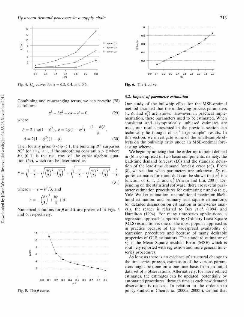
Numerical solutions for �pp and �aa are presented in Figs. 5and 6, respectively.

3.2. Impact of parameter estimation

Our study of the bullwhip effect for the MSE-optimalmethod assumed that the underlying process parameters(s, /, and r2e ) are known. However, in practical imple-mentation, these parameters need to be estimated. Whenconsistent and asymptotically unbiased estimates areused, our results presented in the previous section cantechnically be thought of as ‘‘large-sample’’ results. Inthis section, we investigate some of the small-sample ef-fects on the bullwhip ratio under an MSE-optimal fore-casting scheme.We begin by noticing that the order-up-to point defined

in (6) is comprised of two basic components, namely, thelead-time demand forecast (DDL

t ) and the standard devia-tion of the lead-time demand forecast error (rLe ). From(8), we see that when parameters are unknown, DDL

t re-quires estimates for s and /. It can be shown that rLe is afunction of L, s, /, and r2e (Alwan and Liu, 2001). De-pending on the statistical software, there are several para-meter estimation procedures for estimating s and / (e.g.,Yule–Walker estimation, unconditional maximum likeli-hood estimation, and ordinary least square estimation):for detailed discussion on estimation in time-series anal-ysis, the reader is referred to Box et al. (1994) andHamilton (1994). For many time-series applications, aregression approach supported by Ordinary Least Square(OLS) estimation is one of the most popular approachesin practice because of the widespread availability ofregression procedures and because of many desirableproperties of OLS estimators. The standard estimator ofr2e is the Mean Square residual Error (MSE) which isroutinely reported with regression and more general time-series procedures.As long as there is no evidence of structural change to

the time-series process, estimation of the various param-eters might be done on a one-time basis from an initialdata set of n observations. Alternatively, for more refinedestimates, the estimates can be updated, potentially byautomated procedures, through time as each new demandobservation is realized. In relation to the order-up-topolicy studied in Chen et al. (2000a, 2000b), we find that

Fig. 4. L�oe curves for a ¼ 0:2, 0.4, and 0.6.

Fig. 5. The �pp curve.

Fig. 6. The �aa curve.


Dow

nloa

ded

by [

Cas

e W

este

rn R

eser

ve U

nive

rsity

] at

04:

55 2

3 N

ovem

ber

2014

the authors adopted an approach of continually updatingthe estimate of the standard deviation of the lead-timedemand forecast error (rLe ) where the updating algorithmis based on a moving-average or EWMA scheme, re-spectively. Similarly, we define rrLe;t as the estimate of r

Le

made at time t. Referring to (6), (8), and (9), we recognizethat when parameters are unknown, the ordering variableis given by:

qt ¼ DDLt � DDL

t�1� �þ z rrLe;t � rrLe;t�1

� þ dt;

¼ K1ð//t; sst;LÞ � K1ð//t�1; sst�1; LÞ þ//tð1� //L

t Þð1� //tÞ

þ 1" #

dt

� //t�1ð1� //Lt�1Þ

ð1� //t�1Þdt�1 þ zðrrLe;t � rrLe;t�1Þ; ð32Þ

where //i represents the estimate of / made at time i and

K1ð//i; ssi; LÞ ¼Lð1� //iÞ � //ið1� //L

i Þð1� //iÞ2

ssI : ð33Þ

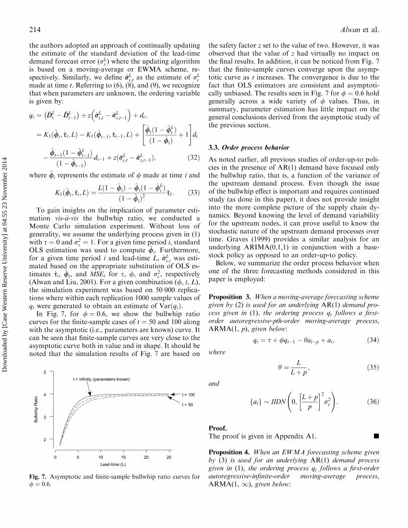
To gain insights on the implication of parameter esti-mation vis-a-vis the bullwhip ratio, we conducted aMonte Carlo simulation experiment. Without loss ofgenerality, we assume the underlying process given in (1)with s ¼ 0 and r2e ¼ 1: For a given time period i, standardOLS estimation was used to compute //i. Furthermore,for a given time period i and lead-time L, rrLe;i was esti-mated based on the appropriate substitution of OLS es-timates ssi, //i, and MSEi for s, /, and r2e , respectively(Alwan and Liu, 2001). For a given combination (/, t, L),the simulation experiment was based on 50 000 replica-tions where within each replication 1000 sample values ofqt were generated to obtain an estimate of VarðqtÞ.In Fig. 7, for / ¼ 0:6, we show the bullwhip ratio

curves for the finite-sample cases of t ¼ 50 and 100 alongwith the asymptotic (i.e., parameters are known) curve. Itcan be seen that finite-sample curves are very close to theasymptotic curve both in value and in shape. It should benoted that the simulation results of Fig. 7 are based on

the safety factor z set to the value of two. However, it wasobserved that the value of z had virtually no impact onthe final results. In addition, it can be noticed from Fig. 7that the finite-sample curves converge upon the asymp-totic curve as t increases. The convergence is due to thefact that OLS estimators are consistent and asymptoti-cally unbiased. The results seen in Fig. 7 for / ¼ 0:6 holdgenerally across a wide variety of / values. Thus, insummary, parameter estimation has little impact on thegeneral conclusions derived from the asymptotic study ofthe previous section.

3.3. Order process behavior

As noted earlier, all previous studies of order-up-to poli-cies in the presence of AR(1) demand have focused onlythe bullwhip ratio, that is, a function of the variance ofthe upstream demand process. Even though the issueof the bullwhip effect is important and requires continuedstudy (as done in this paper), it does not provide insightinto the more complete picture of the supply chain dy-namics. Beyond knowing the level of demand variabilityfor the upstream nodes, it can prove useful to know thestochastic nature of the upstream demand processes overtime. Graves (1999) provides a similar analysis for anunderlying ARIMA(0,1,1) in conjunction with a base-stock policy as opposed to an order-up-to policy.Below, we summarize the order process behavior when

one of the three forecasting methods considered in thispaper is employed:

Proposition 3. When a moving-average forecasting schemegiven by (2) is used for an underlying AR(1) demand pro-cess given in (1), the ordering process qt follows a first-order autoregressive-pth-order moving-average process,ARMA(1, p), given below:

qt ¼ sþ /qt�1 � hat�p þ at; ð34Þwhere

h ¼ LLþ p

; ð35Þ

and

atf g IIDN 0;Lþ pp

� �2r2e

!: ð36Þ

Proof.The proof is given in Appendix A1. j

Proposition 4. When an EWMA forecasting scheme givenby (3) is used for an underlying AR(1) demand processgiven in (1), the ordering process qt follows a first-orderautoregressive-infinite-order moving-average process,ARMA(1, 1), given below:

Fig. 7. Asymptotic and finite-sample bullwhip ratio curves for/ ¼ 0:6.

214 Alwan et al.

Dow

nloa

ded

by [

Cas

e W

este

rn R

eser

ve U

nive

rsity

] at

04:

55 2

3 N

ovem

ber

2014

qt ¼ sþ /qt�1 �X1j¼ 1

hjat�j þ at; ð37Þ

where

hj ¼ La2ð1� aÞj�1Laþ 1 ; ð38Þ

and

atf g IIDN 0; Laþ 1½ �2r2e�

: ð39Þ


Proposition 5. When an MSE-optimal forecasting schemegiven by (5) is used for an underlying AR(1) demand pro-cess given in (1), the ordering process qt follows a first-order autoregressive-first-order moving-average process,ARMA(1, 1), given below:

qt ¼ sþ /qt�1 � hat�1 þ at; ð40Þwhere

h ¼ /ð1� /LÞ1� /Lþ1 ; ð41Þ

and

atf g IIDN 0;1� /Lþ1

1� /

� �2r2e

!: ð42Þ


Among the many reasons why a full characterization ofthe upstream demand process is important is a practicalconcern for the upstream demand nodes in terms of fore-casting their own realized demand processes for orderingfurther up the supply chain stream. Propositions 3–5 giveus insight into the forecasting challenges faced by the up-stream nodes given the forecasting schemes employeddownstream. In particular, we learned that when a mov-ing-average method is used, the next upstream node willexperience an ARMA(1, p) demand process and when anEWMA method is used the next upstream node will ex-perience an ARMA(1,1) demand process. In either case,given the complexity of the demand process in terms of thehigher order moving-average terms (i.e., past error terms),if the upstream node wishes to properly identify the natureof the demand process, it is most likely that mis-specifi-cation of the process will occur. However, when an MSE-optimal forecasting scheme is used on the AR(1) process,the next upstream node benefits from realizing a demandprocess –ARMA(1,1) –which is commonly encountered inpractice and is much simpler to identify (Box et al., 1994).

4. Upstream demand behavior based on an incomingARMA(1,1) demand process

Our previous section analysis revealed that when incom-ing demand follows pure autoregressive behavior, thenext stage of demand inherits the influence of past errorterms, moving-average terms from the general class ofARMA models. Generally speaking, the presence of low-order moving-average terms in real-world processes isquite common. In this section, we will investigate some ofthe implications of introducing moving-average terms. Inparticular, we will study dynamics on the supply chainwhen the incoming demand process is an ARMA(1,1).With respect to the forecasting method, our focus will beon an MSE-optimal scheme.Suppose the system is faced with an ARMA(1,1) de-

mand process given as follows:

dt ¼ sþ /dt�1 � het�1 þ et; ð43Þwhere dt is the observed demand in period t, s > 0,/j j < 1, hj j < 1, and etf g is an iidn process with mean zeroand variance r2e . The condition of hj j < 1 is a standardrestriction on the moving-average parameter and isknown as the invertibility condition. The invertibilitycondition is important for model identification in that itestablishes a one-to-one correspondence between theautocorrelation function and the model (Box et al., 1994).For such a process, MSE-optimal forecast function (i.e.,the conditional expectation of dtþi taken at time t) is givenby:

Ftþi ¼ 1� /i

1� /sþ /idt � h/i�1et for i ¼ 1; 2; . . . ð44Þ

As with the AR(1), the forecasts revert geometricallyback to the overall mean, however, the forecast is modi-fied by a factor depending on the realized forecast error attime t.Using (44), we find for the optimal forecasting method,

the lead-time demand forecast is given by

DDLt ¼

XLi¼ 1

1� /i

1� /sþ /idt � h/i�1et

� �;

¼ Ls� ðLþ 1Þs/þ 2s/2 � bs/Lþ1

ð1� /Þ2

þ /ð1� /LÞð1� /Þ dt � hð1� /LÞ

ð1� /Þ et;

¼ K2ð/; s; LÞ þ /ð1� /LÞð1� /Þ dt � hð1� /LÞ

ð1� /Þ et: ð45Þ

Proposition 6. When an MSE-optimal forecasting schemegiven by (44) is used for an underlying ARMA(1,1) demandprocess given in (43), the ordering process qt follows alsoARMA(1,1) as given below:


Dow

nloa

ded

by [

Cas

e W

este

rn R

eser

ve U

nive

rsity

] at

04:

55 2

3 N

ovem

ber

2014

qt ¼ sþ /qt�1 � h0at�1 þ at; ð46Þwhere

h0 ¼ ð/� hÞ 1� /L� �= 1� /ð Þ þ h

ð/� hÞ 1� /L� �= 1� /ð Þ þ 1 ð47Þ

and

atf g IIDN 0;h/� hð Þ 1� /L� ��

1� /ð Þ�þ 1i2r2e�:

�ð48Þ


Stated in other words, Proposition 6 implies that if theinput demand process follows an ARMA(1,1) process andan MSE-optimal forecasting scheme is used, then the nextupstream stage demand process also follows an ARMA(1,1) process. Interestingly, we learned from Proposition 5that an ARMA(1,1) upstream demand process will alsoresult from an AR(1) input demand process.Combining the results of Propositions 5 and 6, we can

make an interesting extension to a multiple-stage supplychain. Assume that all the stages use an MSE-optimalforecasting scheme in an order-up-to supply-chain envi-ronment. It should be noted that the assumption ofcommon use of an MSE-optimal forecasting schemethroughout the supply chain is not unrealistic in light ofthe earlier noted fact that automatic ARMA fittingpackages are readily available (e.g., AUTOBOX). Fur-thermore, these automatic software can be easily inte-grated into supply chain integrative platforms such asManugistics or SAP.Define the first-stage demand process as the ultimate

customer demand process and subsequent stage demandprocesses as the demand processes as one moves up-stream the supply chain. Under the noted assumptions,we can state that the jth upstream demand process is anARMA(1,1) given as follows:

qt ¼ sþ /qt�1 � hðjÞat�1;j þ at;j; ð49Þwhere

hðjÞ ¼ ½/� hðj�1Þ� 1� /L� �= 1� /ð Þ þ hðj�1Þ

½/� hðj�1Þ� 1� /L� �= 1� /ð Þ þ 1 ðj ¼ 2;3; . . .Þ;

ð50Þand

at;j� � IIDN 0; ½/� hðj�1Þ� 1� /L

1� /

� �þ 1

� �2r2e

!

ðj ¼ 2; 3; . . .Þ; ð51Þwhere r2e is the variance of the error process associatedwith the first-stage demand process and hð1Þ ¼ 0 if the

first-stage demand process is an AR(1) process, otherwisejhð1Þj < 1 if the first-stage demand process is anARMA(1,1) process.

5. Concluding remarks

There is a common perception that improved forecastingtechniques at any one level in the supply chain cannoteliminate the bullwhip effect. This perception is reinforcedwhen studies of the bullwhip effect tend to focus only onsimplified and non-optimal forecasting techniques that, asseen in this paper, are indeed associated with an ever-worsening bullwhip effect as a function of lead-time. Incontrast, we found that in an order-up-to system thebullwhip effect under an MSE-optimal forecasting schemeapproaches a limiting value with lead-time when the de-mand process follows a positively correlated stationaryAR(1) process. Furthermore, it was revealed that there isactually no bullwhip effect for a negatively correlatedprocess under an MSE-optimal forecasting scheme asopposed to the ever-increasing bullwhip effect with lead-time under the moving-average and EWMA methods. Itwas also revealed that parameter estimation in this order-up-to system had limited impact on the general asymptoticresults for the MSE-optimal forecasting scheme.It is worth pointing out that even though this paper

was not meant to be a direct comparison with the pre-vious studies of Chen et al. (2000a, b), the basic results ofthis paper are indeed generally transferable to the order-up-to system studied in Chen et al. (2000a, b). The onlydifference in the order-up-to system of this paper versusChen et al. (2000a, 2000b) is that we did not incorporatea review period in the lead-time. The inclusion of a reviewperiod implies a lead-time of Lþ 1 in terms of how wedefined L in this paper. The adding of constant ‘‘1’’clearly will not change the fundamental facts of convexityof the bullwhip function when simplistic forecastingschemes are used, as in Chen et al. (2000a, b), as opposedto concavity of the bullwhip function when an MSE-op-timal forecasting scheme is used.Beyond the bullwhip effect, the full characterization of

the upstream demand processes was given. This is notonly important from the perspective of having a morecomplete picture of the supply chain dynamics but also isimportant from the practical perspective of recognizingthe forecasting challenges faced by the upstream nodes.Finally, our identification of the upstream demand pro-cess allowed us to reveal an interesting result that undercertain conditions the demand process remains in theform of an ARMA(1,1) as one moves upstream.This paper fills in a missing piece in the landscape of

forecasting model choices for SCM application. Whereasprevious works provided exclusive insight on simplistic,forecasting models, our work provides insights on formaltime-series modeling of demand information versus the

216 Alwan et al.

Dow

nloa

ded

by [

Cas

e W

este

rn R

eser

ve U

nive

rsity

] at

04:

55 2

3 N

ovem

ber

2014

simplistic methods. In summary, with the results of thispaper, operations managers can make an informedchoice. A choice that pins simplicity against operationalbenefits associated with improved forecasting accuracy.

References

Alwan, L.C. (2000) Statistical Process Analysis, McGraw Hill/Irwin,Burr Ridge, IL.

Alwan, L.C. and Liu, J.J. (2001) Accuracy of forecast-facilitated ordersunder AR(1) demand. Working paper, School of Business Ad-ministration, University of Wisconsin-Milwaukee, Milwaukee,WI 53201, USA.

Box, G.E., Jenkins, G.M. and Reinsel, G.C. (1994) Time Series Anal-ysis: Forecasting and Control, 3rd edn., Prentice Hall, EnglewoodCliffs, NJ.

Chen, F., Drezner, Z., Ryan, J.K. and Simchi-Levi, D. (2000a)Quantifying the bullwhip effect in a simple supply chain: the im-pact of forecasting, lead times, and information. ManagementScience, 46, 436–443.

Chen, F., Ryan, J.K. and Simchi-Levi, D. (2000b) The impact of ex-ponential smoothing forecasts on the bullwhip effect. Naval Re-search Logistics, 47, 269–286.

Graves, S.C. (1999) A single-item inventory model for a nonstationarydemand process. Manufacturing and Service Operations Manage-ment, 1, 50–61.

Graves, S.C. and Willems, S.P. (2000) Optimizing strategic safety stockplacement in supply chains.Manufacturing and Service OperationsManagement, 2, 68–83.

Hamilton, J.D. (1994) Time Series Analysis, Princeton UniversityPress, Princeton, NJ.

Hoerl, R.W. (1998) Six sigma and the future of the quality profession.Quality Progress, June, 35–42.

Kahn, J. (1987) Inventories and the volatility of production. TheAmerican Economic Review, 77, 667–679.

Lee, H.L., Padmanabhan, P. and Whang, S. (1997) Information dis-tortion in a supply chain: the bullwhip effect. Management Sci-ence, 43, 546–558.

Lee, H.L., So, K.C. and Tang, C.S. (2000) The value of information sha-ring in a two-level supply chain.Management Science, 46, 626–643.

Shumway, R.H. (1986) AUTOBOX (Version 1.02). The AmericanStatistician, 40, 299–300.

Appendices

Appendix A1: Proof of Proposition 3

Considering (2), (6), and (7), we have the following:

yt ¼ Ldt þ dt�1 þ � � � þ dt�pþ1

p

� �þ zrLe ; ðA1Þ

yt�1 ¼ Ldt�1 þ dt�2 þ � � � þ dt�p

p

� �þ zrLe : ðA2Þ

Replacing (A1) and (A2) in (9), we find:

qt ¼ Lpþ 1

� �dt � L

pdt�p: ðA3Þ

This implies that:

qt�1 ¼ Lpþ 1

� �dt�1 � L

pdt�p�1: ðA4Þ

Now consider replacing dt and dt�p in (A3) with equiva-lent values based on their lag one term along with theerror term as given by Equation (1). When done, weobtain the following:

qt ¼ Lpþ 1

� �dt � L

pdt�p;

¼ Lpþ 1

� �ðsþ /dt�1 þ etÞ � L

pðsþ /dt�p�1 þ et�pÞ;

¼ sþ Lpþ 1

� �/dt�1 þ L

pþ 1

� �et � L

p/dt�p�1 � L

pet�p:

ðA5ÞNow, multiply / times qt�1 as defined by (A4) to obtain:

/qt�1 ¼ Lpþ 1

� �/dt�1 � L

p/dt�p�1: ðA6Þ

Subtracting (A6) from (A5) and then rearranging, wehave:

qt ¼ sþ /qt�1 � Lpet�p þ L

pþ 1

� �et: ðA7Þ

Define at as a random error variable in the followingmanner:

at ¼ Lpþ 1

� �et ¼ Lþ p

pet: ðA8Þ

The independence and normality of at are straightfor-ward results since we are simply multiplying a scalartimes the iidn error term et. In addition, the variance of atas reported in the proposition is immediately apparent.Based on the above error term definition, it can be no-ticed that:

Lpet�p ¼ L

p

� �p

Lþ p

� �at�p;

¼ LLþ p

� �at�p: ðA9Þ

If we define

h ¼ LLþ p

;

and substitute (A8) and (A9) into (A7), we obtain thereported time-series model for qt. j


By means of recursive substitution, we can re-write (3) as:

Ftþ1 ¼ aX1j¼0

ð1� aÞjdt�j: ðA10Þ


Dow

nloa

ded

by [

Cas

e W

este

rn R

eser

ve U

nive

rsity

] at

04:

55 2

3 N

ovem

ber

2014

By applying (A10) to (7) and then, in turn, to (6), weobtain:

yt ¼ LaX1j¼0

ð1� aÞjdt�j þ zrLe ; ðA11Þ

yt�1 ¼ LaX1j¼0

ð1� aÞjdt�1�j þ zrLe : ðA12Þ

By expanding out (A11) and (A12) and applying the ex-pansions to (9), we have:

qt ¼ L½aðdt � dt�1Þ þ að1� aÞðdt�1 � dt�2Þþ að1� aÞ2ðdt�2 � dt�3Þ þ � � �� þ dt: ðA13Þ

This implies that:

qt�1 ¼ L½aðdt�1 � dt�2Þ þ að1� aÞðdt�2 � dt�3Þþ að1� aÞ2ðdt�3 � dt�4Þ þ � � �� þ dt�1: ðA14Þ

Now consider replacing dt�i in (A13) with equivalentvalues based on their lag one term along with the errorterm as given by Equation (1). When done, we obtain thefollowing:

qt ¼ L½aðsþ /dt�1 þ et � s� /dt�2 � et�1Þþ að1� aÞðsþ /dt�2 þ et�1 � s� /dt�3 � et�2Þþ � � �� þ sþ /dt�1 þ et;

¼ /L½aðdt�1 � dt�2Þ þ að1� aÞðdt�2 � dt�3Þþ að1� a2Þðdt�3 � dt�4Þ þ � � �� þ L½aðet � et�qÞþ að1� aÞðet�1 � et�2Þ þ að1� a2Þðet�2 � et�3Þþ � � �� þ sþ /dt�1 þ et: ðA15Þ

Now, multiply / times qt�1 as defined by (A14) to obtain:

/qt�1 ¼ /L½aðdt�1 � dt�2Þ þ að1� aÞðdt�2 � dt�3Þþ að1� aÞ2ðdt�3 � dt�4Þ þ � � �� þ /dt�1:

ðA16ÞSubtracting (A16) from (A15) and then rearranging, wehave:

qt ¼ sþ /qt�1 þ et þ L½aðet � et�qÞ þ að1� aÞðet�1 � et�2Þþ að1� a2Þðet�2 � et�3Þ þ � � ��;

¼ sþ /qt�1 þ LX1j¼1

½að1� aÞj � að1� aÞj�1�et�j þ ðLaþ 1Þet;

¼ sþ /qt�1 �X1j¼1

La2ð1� aÞj�1et�j þ ðLaþ 1Þet: ðA17Þ


at ¼ ðLaþ 1Þet: ðA18ÞThe independence and normality of at are straightfor-ward results since we are simply multiplying a scalar

times the iidn error term et. In addition, the variance of atas reported in the proposition is immediately apparent.Based on the above error term definition, it can be no-ticed that:

La2ð1� aÞj�1et�j ¼ La2ð1� aÞj�1Laþ 1

!at�j: ðA19Þ

If we define

hj ¼ La2ð1� aÞj�1Laþ 1 ;




k ¼ /ð1� /LÞ1� /

: ðA20Þ

This allows us to write (16) as:

qt ¼ ðk þ 1Þdt � kdt�1: ðA21Þ

This implies that:

qt�1 ¼ ðk þ 1Þdt�1 � kdt�2: ðA22ÞNow consider replacing dt and dt�1 in (A21) with equi-valent values based on their lag one term along with theerror term as given by Equation (1). When done, weobtain the following:

qt ¼ ðk þ 1Þdt � kdt�1;

¼ ðk þ 1Þðsþ /dt�1 þ etÞ � kðsþ /dt�2 þ et�1Þ;¼ sþ /ðk þ 1Þdt�1 � /kdt�2 � ket�1 þ ðk þ 1Þet: ðA23Þ

Now, multiply / times qt�1 as defined by (A22) to obtain:

/qt�1 ¼ /ðk þ 1Þdt�1 � /kdt�2: ðA24ÞSubtracting (A24) from (A23) and then rearranging, wehave:

qt ¼ sþ /qt�1 � ket�1 þ ðk þ 1Þet: ðA25ÞDefine at as a random error variable in the followingmanner:

at ¼ ðk þ 1Þet ¼ /ð1� /LÞ1� /

þ 1� �

et ¼ 1� /Lþ1

1� /

� �et:

ðA26Þ

The independence and normality of at are straightforwardresults since we are simply multiplying a scalar times theiidn error term et. In addition, the variance of at as re-ported in the proposition is immediately apparent. Basedon the above error term definition, it can be noticed that:

218 Alwan et al.

Dow

nloa

ded

by [

Cas

e W

este

rn R

eser

ve U

nive

rsity

] at

04:

55 2

3 N

ovem

ber

2014

ket�1 ¼ kk þ 1� �

at�1 ¼ /ð1� /LÞ= 1� /ð Þ/ 1� /L� �

= 1� /ð Þ þ 1

!at�1

¼ /ð1� /LÞ1� /Lþ1

� �at�1: ðA27Þ

If we defineh ¼ /ð1� /LÞ

1� /Lþ1




c ¼ 1� /L

1� /: ðA28Þ

This allows us to write the order-up-to point of (6) basedon (45) as:

yt ¼ K2ð/; s; LÞ þ /cdt � hcet þ zrLe : ðA29Þ

Applying (A29) to (9), we obtain:

qt ¼ K2ð/; s; LÞ þ /cdt � hcet � K2ð/; s; LÞ� /cdt�1 þ hcet�1 þ dt;

¼ ð/cþ 1Þdt � /cdt�1 � hcet þ hcet�1: ðA30ÞThis implies that:

qt�1 ¼ ð/cþ 1Þdt�1 � /cdt�2 � hcet�1 þ hcet�2: ðA31ÞNow consider replacing dt and dt�1 in (A30) with equi-valent values based on their lag one term along with theerror term as given by Equation (1). When done, weobtain the following:

qt ¼ ð/cþ 1Þdt � /cdt�1 � hcet þ hcet�1;¼ ð/cþ 1Þðsþ /dt�1 � het�1 þ etÞ � /cðsþ /dt�2

� het�2 þ et�1Þ � hcet þ hcet�1;¼ sþ /ð/cþ 1Þdt�1 � /2cdt�2 � /hcet�1 � het�1þ ð/c� hcþ 1Þet þ /hcet�2 � ð/c� hcÞet�1: ðA32Þ

Now, multiply / times qt�1 as defined by (A31) to obtain:/qt�1 ¼ /ð/cþ 1Þdt�1 � /2cdt�2 � /hcet�1 þ /hcet�2:

ðA33ÞSubtracting (A33) from (A32) and then rearranging, wehave:

qt ¼ sþ /qt�1 � ½ð/� hÞcþ h�et�1 þ ½ð/� hÞcþ 1�et:ðA34Þ


at ¼ ½ð/� hÞcþ 1�et ¼ ð/� hÞ 1� /L

1� /

� �þ 1

� �et:

ðA35Þ

The independence and normality of at are straightfor-ward results since we are simply multiplying a scalartimes the iidn error term et. In addition, the variance of atas reported in the proposition is immediately apparent.Based on the above error term definition, it can be no-ticed that:

½ð/� hÞcþ h�et�1 ¼ ð/� hÞcþ hð/� hÞcþ 1� �

at�1

¼ ð/� hÞ ð1� /LÞ=ð1� /Þ� �þ h

ð/� hÞ ð1� /LÞ=ð1� /Þ� �þ 1 !

at�1

ðA36ÞIf we define

h0 ¼ ð/� hÞ ð/� hLÞ=ð1� /Þ� �þ h

ð/� hÞ ð1� /LÞ=ð1� /Þ� �þ 1 ;and substitute (A35) and (A36) into (A34), we obtain thereported time-series model for qt. j

Biographies

Layth C. Alwan is an Associate Professor at the School of BusinessAdministration, University of Wisconsin-Milwaukee and Co-Directorof the Consortium for Innovative Manufacturing and OperationsManagement. He has earned a B.A. in Mathematics, B.S. in Statistics,M.B.A., and Ph.D. in Business Statistics/Operations Management allfrom the University of Chicago and a M.S. in Computer Science fromDePaul University. His primary research interests are developingmodel-based approaches for more effective statistical process moni-toring and studying the impact of forecasting techniques on opera-tional management. He has published in journals such asCommunications in Statistics, IIE Transactions, Journal of Business andEconomic Statistics, Journal of Management, Journal of the RoyalStatistical Society, and Quality Engineering. He is a member of ASA,INFORMS, IIE, and RSS.

John Liu is a Professor at the School of Business Administration,University of Wisconsin-Milwaukee, and Director of the Consortiumfor Innovative Manufacturing and Operations Management. He re-ceived his M.S. degree in Engineering-Economic Systems from Stan-ford University and Ph.D. degree in Industrial Engineering from thePennsylvania State University. His primary research interests are sto-chastic optimization models, and manufacturing and distribution sys-tems. His current research focuses on time-series modeling andsimulation analysis of supply chain management, and dynamic gamesin innovative manufacturing. He has published in journals such asOperations Research, Management Science, IEEE Transactions on En-gineering Management, the European Journal of Operational Research,and the Journal of Production and Operations Management. He is amember of INFORMS and IIE.

Dong-Qing Yao is an Assistant Professor of Management at TowsonUniversity. He received his B.S. in Industrial Engineering from SuzhouUniversity, and aM.S. in Systems Engineering from Shanghai Jiao TongUniversity, China. He received his Ph.D. in Management Science fromthe University ofWisconsin-Milwaukee. His research interests are in theareas of supply chain management. He is a member of INFORMS.

Contributed by the Engineering Statistics and Applied Probability De-partment


Dow

nloa

ded

by [

Cas

e W

este

rn R

eser

ve U

nive

rsity

] at

04:

55 2

3 N

ovem

ber

2014

Documents

Stochastic characterization of upstream demand processes in a supply chain