Embed Size (px)
Citation preview
Stochastic Declustering of Space-TimeEarthquake Occurrences
Jiancang Zhuang Yosihiko Ogata and David Vere-Jones
This article is concerned with objective estimation of the spatial intensity function of the background earthquake occurrences from anearthquake catalog that includes numerous clustered events in space and time and also with an algorithm for producing declusteredcatalogs from the original catalog A space-time branching process model (the ETAS model) is used for describing how each eventgenerates offspring events It is shown that the background intensity function can be evaluated if the total spatial seismicity intensity andthe branching structure can be estimated In fact the whole space-time process is split into two subprocesses the background events andthe clustered events The proposed algorithm combines a parametric maximum likelihood estimate for the clustering structures using thespace-time ETAS model and a nonparametric estimate of the background seismicity that we call a variable weighted kernel estimate Todemonstrate the present methods we estimate the background seismic activities in the central region of New Zealand and in the centraland western regions of Japan then use these estimates to produce catalogs of background events
KEY WORDS Background seismicity Branching processes Earthquake declustering Space-time ETAS model Thinning methodVariable weighted kernel estimate
1 INTRODUCTION
The motivation of this article arises from problems in theprediction of large earthquakes with clusters of aftershocksThe earthquake clusters complicate the statistical analysisof the background seismic activity that might be related tochanges in the tectonic eld The cluster features differ fromplace to place and typically lie between two extreme types ofspatial clusters of earthquakes those that eventually decreasein time such as aftershock sequences and swarms and thosethat persist in time at the same location Ultimately the persis-tent background activity prevails over the aftershock activityTo forecast the location of the large earthquakes it is neces-sary to analyze the background seismicity for which removalof temporal cluster members is considered to be of centralimportance
A number of methods have been proposed for decluster-ing a catalog to obtain the background seismicity Most ofthese methods remove the earthquakes in a space-time win-dow around a large event called the mainshock the differ-ences among these methods relate to the choice of the windowsizes and some other detailed procedures (see eg Utsu 1969Gardner and Knopoff 1974 Kellis-Borok and Kossobokov1986) In general the bigger the magnitude of the mainshockthe larger the window An alternative to the window-baseddeclustering methods is the link method based on a space-timedistance between the events (eg Resenberg 1985 Frohlichand Davis 1990 Davis and Frohlich 1991)
Jiancang Zhuang is a graduate student Department of Statistical SciencesGraduate University for Advanced Studies 4-6-7 Minami-Azabu Minato-ku106-8569 Tokyo Japan (E-mail zhuangjcismacjp) Yosihiko Ogata is Pro-fessor Institute of Statistical Mathematics 4-6-7 Minami Azabu Minato-ku106-8569 Tokyo Japan (E-mail ogataismacjp) David Vere-Jones is Emer-itus Professor School of Mathematics and Computing Sciences Victoria Uni-versity of Wellington New Zealand The study was initialized while the rstauthor was a visitor to School of Mathematical and Computing Sciences Vic-toria University of Wellington supported by International Cooperation Fundof the China Seismological Bureau and an Earthquake Forecasting subcon-tract with Institute of Geological and Nuclear Sciences in New Zealand Itwas continued with the support of grant-in-aid 11680334 for the Scienti cResearch from the Ministry of Education Science Sport and Culture JapanThis study was also supported by a research fund of Yoshiyasu Tamura Theauthors thank Ma Li for her continuous encouragement and support Theauthors also gratefully acknowledge the assistance of Ray Brownrigg DavidHarte Makoto Taiji and Koichi Katsura as well as the helpful comments andencouragement from the referees and the editor
All of the aforementioned conventional methods containarbitrary parameters for de ning the aftershock window sizesor the link distances in both space and time Each choice ofparameter gives a different declustered catalog and thus a dif-ferent estimate of the background seismicity As a result theconventional declustering algorithms have dif culty makingan optimal choice of parameters For a dataset from a speci c(rather narrow) seismic region and a given threshold magni-tude these choices are usually colored by the userrsquos subjectiveimpression of the declustered output Also given a datasetthe concept of what constitutes an aftershock has not beenuniquely de ned These are among the reasons why so manydifferent declustering algorithms have been proposed
To avoid such dif culties it seems to us inevitable that thedeclustering method should be based on a stochastic model toobjectively quantify the observations so that any given eventhas a probability to be either a background event or an off-spring (cluster) event generated by others Therefore the maintask of a declustering method is to estimate this probabil-ity for each event Several authors have proposed space-timemodels for the way in which earthquakes generate clusteredevents To t their models to Italian historical data Musmeciand Vere-Jones (1992) assumed that the background seismic-ity was proportional to a kernel estimate obtained from thespatial locations of all earthquakes that include clusters Ogata(1998) suggested a space-time version of the epidemic-typeaftershock sequence (ETAS) model He used a conventionaldeclustering algorithm for preliminary estimation of the back-ground rate by tting bicubic B-spline functions before ttingthe space-time ETAS model to all the events However as weshow in this article the use of such a preliminary declusteringmethod can be avoided
In the next section we give a formulation of the space-timepoint process for earthquake occurrences and then investigatesthe relationship between the total spatial rate the backgroundrate and the branching structure of this model This rela-tionship suggests an approach to objective methods for esti-
copy 2002 American Statistical AssociationJournal of the American Statistical Association
June 2002 Vol 97 No 458 Applications and Case Studies
369
370 Journal of the American Statistical Association June 2002
mating the background intensity We discuss several techni-cal methods for carrying out such estimation including thethinning (random deletion) method and a variable bandwidthkernel function method associated with maximum likelihoodestimation of the space-time ETAS model We then obtain thebackground intensity using an iterative algorithm and gener-ate the declustered catalogs Finally we apply this procedureto datasets from the central region of New Zealand and thewestern and central Honshu area of Japan to demonstrate ourmethods
2 SPACEndashTIME MODELS FOREARTHQUAKE OCCURRENCE
Several space-time point-process models have been pro-posed for describing clustering phenomena in seismic activity(Kagan 1991 Musmeci and Vere-Jones 1992 Rathbun 1993Ogata 1998) These models have common features that can beoutlined as follows
(a) The background events are regarded as the ldquoimmi-grantsrdquo in the branching process of earthquake occurrencetheir occurrence rate is assumed to be a function of spatiallocation and magnitude but not of time
(b) Each ldquoancestorrdquo event produces offspring indepen-dently The expected number of direct offspring from an indi-vidual ancestor is assumed to depend on its magnitude M andis denoted by Š4M5
(c) The probability distribution of the time until the appear-ance of an offspring event is a function of the time lag fromits direct ancestor and is independent of magnitude (cf Utsu1962) thus its probability density function is assumed to havethe form g4tmdashrsquo5 D g4t ƒ rsquo5 where rsquo is the occurrence time ofthe ancestor Moreover the function is independent of whathappens between rsquo and t
(d) The probability distributions of the location 4x1 y5 andmagnitude M of an offspring event are dependent on themagnitude M uuml and the location 41 Dagger5 of its direct ances-tor These probability density functions are denoted by f4x ƒ1 y ƒ DaggermdashM uuml 5 and j4M mdashM uuml 5 where Dagger represents the loca-tion and M uuml represents the magnitude of the ancestor
In general this class of marked branching point processesfor earthquake occurrences can be represented completely bythe conditional intensity function (eg Daley and Vere-Jones1988 chap 13) de ned by
Prcopyan event in 6t1 t C dt5 6x1 x C dx5
6y1 y C dy5 6M1M C dM5 mdash umlt
ordf
D lsaquo4t1 x1 y1M mdash umlt5 dt dx dy dM
Co4dt dx dy dM51 (1)
provided that it exists where umlt denotes the space-time mag-nitude occurrence history of the earthquakes up to time tNote that here umlt is the history of the available earthquakerecords including not only those during the study period andin the study area but also those before the study period (egOgata 1992) and outside of the study area (eg this article)In particular we include information about large earthquakes
from outside the study area if they contribute substantially tothe seismicity of the study region during the study period
Based on the assumptions andashd the conditional intensityfunction for the space-time model can be written as
lsaquo4t1 x1 y1M mdash umlt5 D Œ4x1 y1M5 CX
8k2 tkltt9
Š4Mk5g4t ƒ tk5
f 4x ƒ xk1 y ƒ ykmdashMk5j4M mdashMk50 (2)
In this equation Œ4x1 y1M5 is the background intensity func-tion and is assumed to be independent of time The functionsg4t5 f 4x1 ymdashMk5 and j4M mdashMk5 are the normalized responsefunctions (ie pdfrsquos) of the occurrence time location andmagnitude of an offspring from an ancestor of magnitudeMk From the fact that the kth event excites a nonstationaryPoisson process with intensity function Š4Mk5g4t ƒ tk5f 4x ƒxk1 y ƒ yk
mdashMk5j4M mdashMk5 it is easy to see that Š4Mk5 is theexpected number of offspring from an ancestor of size MkNote also that the probability function g4t5 is independent ofthe magnitude of the ancestor as mentioned in assumption c
To simplify the subsequent discussion we also make thefollowing stronger assumption
(e) The magnitude distribution of a background eventis independent of its location so that Œ4x1 y1M5 DŒ4x1 y5jŒ4M5 the magnitude distribution of a direct off-spring event is independent of the size of its ancestor sothat j4M mdashM uuml 5 D j4M5 and the magnitude distributions for thebackground events and their offspring are identical that isjŒ4M5 D j4M5
Under these conditions the conditional intensity function forthe model can be decomposed as
lsaquo4t1 x1 y1 M mdash umlt5 D j4M5lsaquo4t1x1 y mdash umlt51 (3)
where
lsaquo4t1 x1 y mdash umlt5 D Œ4x1 y5 CX
8k2 tkltt9
Š4Mk5g4t ƒ tk5
f4x ƒ xk1 y ƒ ykmdashMk50 (4)
Later in applications we make use of the speci c functionforms
Š4M5 D Ae4MƒM05
g4t5 D(
4p ƒ 15cpƒ14t C c5ƒp for t gt 0
0 otherwise1
and
f 4x1 ymdashM5 D 1
2 de4MƒM05exp ƒ 1
2
x2 C y2
de4MƒM05
as an example These constitute one form of the space-timeETAS model (Ogata 1998 see also Rathbun 1993 for a similarform)
Given an estimated intensity function u4x1y5 we set
Œ4x1 y5 D u4x1y5
Zhuang Ogata and Vere-Jones Stochastic Declustering 371
for the background rate in (4) where is a positive-valuedparameter and maximize the log-likelihood function
logL4Egrave5 DNX
kD1
loglsaquoEgrave4tk1 xk1 ykmdash umltk
5
ƒZ T
0
ZZ
S
lsaquoEgrave4t1 x1 y mdash umlt5 dx dy dt (5)
to obtain the maximum likelihood estimates (MLEs) OEgrave D4 O1 bA1 O1 Oc1 Op1 Od5 where the subscript k runs over all of theevents occurring in the study region S and the study timeinterval 601T 7 Computational details have been given byOgata (1998)
Now assuming stationarity and ergodicity of the space-timepoint process the total spatial intensity function ( rst-ordermoment density) is equal to
m14x1 y5 D limT ˆ
1T
Z T
0lsaquo4t1 x1 y mdash umlt5 dt1 (6)
where T is the length of the observation period Replacing thelimit in (6) by a nite approximation and substituting (4) in(6) we obtain
m14x1 y51T
Z T
0Œ4x1 y5 C
X
8k2 tkltT 9
Š4Mk5g4t ƒ tk5
f 4x ƒ xk1 y ƒ ykmdashMk5 dt
D Œ4x1 y5 C 1T
X
8k2 tkltT 9
Š4Mk5f 4x ƒ xk1 y ƒ ykmdashMk5
Z T
tk
g4t ƒ tk5 dt
D Œ4x1 y5 C 1T
X
8k2 tkltT 9
Š4Mk5
f 4x ƒ xk1 y ƒ ykmdashMk50 (7)
Therefore an estimator of the background intensity can bederived from
Œ4x1 y5 m14x1 y5 ƒ 1T
X
8k2 tkltT 9
Š4Mk5f 4x ƒ xk1 y ƒ ykmdashMk51
(8)
where both the total rate m14x1 y5 and the transfer functionŠ4M5f 4x1 ymdashM5 can be estimated
3 THINNING PROCEDURE
To obtain a practical version of (8) we consider the fol-lowing thinning operation (or random deletion) Consider aseries of events 84tj1 xj1 yj 52 j D 1121 1N 9 associated witha series of probabilities 8j 2 j D 1121 1N 9 Suppose thateach event j of this process is deleted with probability j Then the remaining events represent a new point processcalled the thinned process The simplest form of the thin-ning operation is to delete each point with a xed probability(eg Daley and Vere-Jones 1972) The thinning method has
also been used for the simulation of point processes (see egLewis and Shedler 1979 Ogata 1981 1998 Musmeci andVere-Jones 1992)
Here we interpret j as the probability of the jth earthquakebeing an offspring in the process de ned as follows In thesecond term in (4) we set
i1jD Pr 8the jth event is an offspring of ith eventmdashumltj
9
D Š4Mi5g4tjƒ ti5f 4xj
ƒ xi1 yjƒ yi
mdashMi5
lsaquo4tj1 xj1 yjmdash umltj
5(9)
and
jD Pr 8the jth event to be an offspringmdashumltj
9
Djƒ1X
iD1
i1j1 (10)
where j micro 1 because it represents the ratio of the sum termin (4) to the whole of (4) Thus the probability that the jthevent belongs to the background is
jD Pr 8the jth event is an immigrant mdash umltj
9
D 1ƒ jD
Œ4xj1 yjmdashumltj
5
lsaquo4tj1 xj1 yjmdash umltj
50 (11)
If we delete the jth event in the process with probability j
for all j D 1121 1N then the thinned process should real-ize a nonhomogeneous Poisson process of the spatial intensityŒ4x1 y5 (see Ogata 1981 for the justi cation) We call this pro-cess the background subprocess and call the complementarysubprocess the cluster subprocess or the offspring process
4 VARIABLE KERNEL ESTIMATESOF SEISMICITY
Estimating the mean rate m14x1 y5 of the total seismic activ-ity in (8) can be carried out by several methods includingusing kernel estimates (eg Vere-Jones 1992) or spline func-tions (eg Ogata and Katsura 1988) Here we adopt the ker-nel estimate method The simple kernel estimate with a xedbandwidth has a serious disadvantage however For a spatiallyclustered point dataset a small bandwidth gives a noisy esti-mate for the sparsely populated area whereas a large band-width mixes up the boundaries between the densely populatedand sparsely populated areas Therefore instead of the kernelestimate
Om14x1 y5 D 1T
NX
jD1
kd4x ƒ xj1 y ƒ yj51 (12)
where kd4x1 y5 denotes the Gaussian kernel function
kd4x1 y5 D 12 d
exp ƒ x2 C y2
2d2
with a xed bandwidth d we adopt
Om14x1 y5 D 1T
NX
jD1
kdj4x ƒ xj 1 y ƒ yj 51 (13)
372 Journal of the American Statistical Association June 2002
where dj represents the varying bandwidth calculated for eachevent j in the following way Given a suitable integer np
between 10 and 100 nd the smallest disk centered at thelocation of the jth event that includes at least np other earth-quakes and with a radius larger than some small value (eg adistance within 002 degree which is of the order of the loca-tion error) and let its radius be dj (eg Silverman 1986 chap5) Similar ideas have been given by Choi and Hall (1998)and Musmeci and Vere-Jones (1986)
Using the same kernel function kdjas in (13) the occur-
rence rates of the cluster and background subprocesses canthen be estimated by
Oƒ4x1 y5 D 1T
Xj
jkdj4x ƒ xj1 y ƒ yj51 (14)
where j is derived from (10) and
OŒ4x1y5D Om14x1y5ƒ Oƒ4x1y5D 1T
Xj
41ƒj5kdj4xƒxj1yƒyj50
(15)
We call the estimates in (14) and (15) the variable weightedkernel estimates
There remains the problem of optimal selection of np forthe variable bandwidth for the statistics in (13) (14) and (15)Remembering that the clustering intensity term on the rightside of (8)
IT 4x1 y5 D 1T
X
j
Š4Mj5f 4x ƒ xj1 y ƒ yjmdashMj51 (16)
is also an image of the clustering intensity in space but not sosmoothed we can in principle select a suitable np for Oƒ4x1 y5
by minimizing the discrepancy between the low-frequency(smoothed) component of IT 4x1 y5 in (16) and Oƒ4x1 y5 in (14)In practice the estimates are rather insensitive to the choiceof np so that a rough estimate is generally suf cient Atthe same time the mean rate Om14x1 y5 is also compared toR T
0Olsaquo4t1 x1 ymdashumlt5 dt=T in view of (7) where 601T 7 is the obser-
vation time interval
5 ITERATION ALGORITHM
In Sections 2ndash4 we outlined methodologic solutions to thefollowing issues (a) how to obtain the MLE of the space-timeETAS model for the branching structure when the backgroundrate is given (b) how to estimate the total spatial occurrence
Table 1 Convergence Steps of the Evaluation Procedure in Applying the Space-Time ETAS Modelby Algorithm 1 to the Earthquake Data From the Central New Zealand Region
log L A c p d
1 ƒ7987049 043594 43378 024737 73554 11573 039395e ƒ 022 ƒ7716051 1025850 31482 016264 93397 11671 019980e ƒ 023 ƒ7710075 095684 33944 017698 88535 11638 023097e ƒ 024 ƒ7696038 1000945 33370 017370 89776 11644 022326e ƒ 025 ƒ7695060 099755 33492 017441 89518 11643 022487e ƒ 026 ƒ7694069 1000011 33465 017426 89574 11643 022452e ƒ 027 ƒ7694088 099955 33471 017429 89562 11643 022459e ƒ 028 ƒ7694084 099966 33470 017428 89565 11643 022458e ƒ 02
rate and (c) how to estimate the background seismicity in thecase where the branching structure is provided But in real-ity we know only the earthquake datamdashnamely the records ofoccurrence times locations and magnitudes of the observedevents To estimate the background rate from these data onlywe carry out the following iterative algorithm that simultane-ously estimates the background rate and the branching struc-ture
Algorithm 1
1 Given a preliminary parameter np say 20 calculatethe bandwidth dj for each event 4tj1 xj1 yj1Mj5 j D11 21 001N
2 Set l D 0 and u4054x1 y5 D 13 Using the maximum likelihood procedure described by
for example Ogata (1998) t the conditional intensityfunction
lsaquo4t1 x1 ymdashumlt5 D u4l54x1 y5 CX
k2 tkltt
Š4Mk5g4t ƒ tk5
f 4x ƒ xk1 y ƒ ykmdashMk5 (17)
to the earthquake data where k g and f are de nedafter (4)
4 Calculate j from (9) and (10) for each j D 1 21 1N 5 Calculate OŒ4x1 y5 from (15) and record as u4lC154x1 y56 If max4x1y5
mdashu4lC154x1 y5 ƒ u4l54x1 y5mdash gt ˜ where ˜ is asmall positive number then set l D lC1 and go to step 3Otherwise take Ou4lC154x1 y5 as the background rate andstop
The np is tuned so as to nd the value that can minimizethe difference between the low-frequency part of IT 4x1 y5 andOƒ4x1 y5 In this study we nd that the adjustment of np is notso sensitive for the nal estimates of Om14x1 y5 and Oƒ4x1 y5comparing to
R T
0Olsaquo4t1x1 y5 dt and IT 4x1 y5 The estimates only
change slightly when np changes in the range of 15ndash100 Inthis article we adopt np
D 20 as a standard value for use withthe New Zealand and Japanese data
This algorithm converges quickly Table 1 shows anexample of the convergence steps of this algorithm when thespace-time ETAS model in (4) was applied to the earthquakedata from the central New Zealand region which is discussedin the next section
Zhuang Ogata and Vere-Jones Stochastic Declustering 373
6 APPLICATIONS
61 Central New Zealand Region
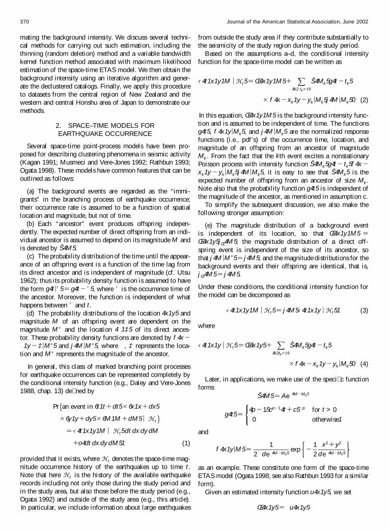
The data used in this calculation are from the New Zealandlocal catalog recorded by the Institute of Geology and NuclearSciences For this study we select the earthquake data for theperiod January 1970ndashAugust 1999 from the rectangular area38ndash43S and 171ndash179E (the central New Zealand region)which extends from the boundary of the Bay of Plenty toArthurrsquos Pass (Fig 1) We take the magnitude threshold ML
D400 and consider shallow events down to the depth of 40 km
The nal MLE values of the space-time ETAS modelfor this subregion are bA D 033470 event(deg2 day) O D0895651 Oc D 0017428 day Op D 101643 and Od D 00022458deg2From here on we use deg2 to denote the unit of the geograph-ical area where the unit degree is that of latitude (11111 km)The converging steps of the calculation are shown in Table 1
Figure 2(a) shows the temporal change of the function
p4t5 DRR
SOlsaquo4t1 x1 ymdashumlt5 dx dyRR
SOŒ4x1 y5 dx dy
1 (18)
that is the integrated conditional intensityRR
SOlsaquo4t1 x1
ymdashumlt5 dx dy over the whole study region S relative to theoverall background rate
RRS
OŒ4x1 y5 dx dy The pattern is sim-ilar to that from the simple ETAS model (Ogata 1988)Figure 2(b) shows the total intensity Om14x1 y5 of the centralNew Zealand region Figure 2(c) shows the spatial clusteringintensity Oƒ4x1 y5 calculated by (14) To enhance the contrastbetween Figures 2(b) and (c) we introduce the concept ofrelative clustering effect which is shown by the contours inFigure 2(d) We do this to measure the cluster effect relativeto the overall rate and de ned by the ratio of the spatial clus-tering intensity to the total intensity that is
C4x1 y5 DOƒ4x1 y5
Om4x1 y5D
Pj jkdj
4x ƒ xj1 y ƒ yj5Pj kdj
4x ƒ xj1 y ƒ yj50 (19)
Here C4x1 y5 can be regarded as a smoothed value of j
(a)
43
o4
2o
41
o4
0o
39
o3
8oS
170o
172o
174o
176o
178oE rsquo70 rsquo75 rsquo80 rsquo85 rsquo90 rsquo95
(b)
43
o4
2o
41
o4
0o
39
o3
8oS
Figure 1 Epicentral Locations in the Central New Zealand Region (a) and Space-Time Plots for the Latitudes Against the Times of All of theEvents (b)
Figures 2(b)ndash(d) show that most places in the study areahave a total intensity of less than 50 eventsdeg2 through-out the whole period of 2875 years (T D 101500 days) Theclustering intensity is less than 20 eventsdeg2 throughout theperiod and the relative clustering effect is less than 3 Somespots get high values for these three quantities however Theyare located mainly in the plate boundary between the Paci cand Australian plates or in the inland volcanic zones
By subtracting the clustering intensity from the overallintensity as indicated in (15) we can get the estimate of thebackground intensity function shown in Figure 2(e) It can beseen that the background rate is much smoother than the totalrate in Figure 2(b) Most places have values in the range of20ndash50 eventsdeg2 except for the plate boundary where thehigh values form up a strip with values of 50ndash100 eventsdeg2
and some peaks up to 200 eventsdeg2 Also some high valuesare seen in the volcanic zones and offshore from Wanganui
62 Central and Western Japan
The second example used data from the central and westernHonshu area of Japan from the hypocenter catalog compiledby the Japan Meteorological Agency (Fig 3) We selecteddata for the period 1926ndash1995 in the rectangular area 34ndash39N and 131ndash140E with magnitudes MJ para 400 and depthsmicro100 km Outside the southern boundary were two greatearthquakes the 1944 Tonankai earthquake of MJ 79 with epi-center (13662E 3380N) and the 1946 Nankai earthquake ofMJ 80 with epicenter (13562E 3303N) These events andtheir large aftershocks apparently affected the seismic activ-ity in the aforementioned selected inland area However thedetection rate of earthquakes offshore is quite low comparedto that inland and thus it is hard to widen the region of theanalysis without raising the threshold magnitude substantiallyInstead we keep the same area and same magnitude thresholdas before for the analysis but allow for boundary effects aris-ing from the occurrence of the earthquakes not more than 1degree outside the study area to include the in uence of thetwo great events with magnitude para708 Thus the likelihoodcalculation is implemented for the enlarged history umlt con-taining data from the extended region
374 Journal of the American Statistical Association June 2002
Time (Year)
Rel
ativ
e in
tens
ity
(a)
110
100
rsquo70 rsquo72 rsquo74 rsquo76 rsquo78 rsquo80 rsquo82 rsquo84 rsquo86 rsquo88 rsquo90 rsquo92 rsquo94 rsquo96 rsquo98
1
5
5
10
10 1
0
20 20
50
50
50
50
50
50
50
100
100
100
200
170 172 174 176 178 Eo o o o o
(b)
4342
4140
3938
So
oo
oo
o
1
1
1
5
5
5
5
10
10 10
10
10
20
20
20
20
20
20
20
50
50
50
50
50
50
100
170 172 174 176 178 Eo o o o o
(c)
4342
4140
3938
So
oo
oo
o
02
02
02
02
02
02
02
04
04
04
04
04
04
04
06
06
06
08
170 172 174 176 178 Eo o o o o4342
4140
3938
So
oo
oo
o
(d)
1
5
5
10
10 20
20
20
50 50
50
50
50
100
100
170 172 174 176 178 Eo o o o o4342
4140
3938
So
oo
oo
o
(e)
Figure 2 Results From the Central New Zealand Region (a) Plot of the conditional intensity function of time integrated over the studied regionThe horizontal axis represents time in years and the vertical axis represents the ratio of the conditional intensity to the background intensity overthe whole region (b) Contours of the estimated total rate Om1( x y) [see (13)] (c) The clustering intensity Oƒ( xy ) [see (14)] (d) The estimatedrelative clustering effect bC( x y) [see (19)] (e) The estimated background seismicity rate OŒ(x y ) [see (15)] In (b) (c) and (e) the values are ineventsdeg2 throughout the whole period (T D 10 500 days) and contours are drawn for approximately equal intervals in a logarithmic scale Thethick solid lines represent the coastlines
132o 134o 136o 138o 140oE34o
35o
36o
37o
38o
39o N
(a) (b)
132o 134o 136o 138o 140oE
rsquo30
rsquo45
rsquo60
rsquo75
rsquo90
Figure 3 Epicentral Locations and Selected Subregions in the Western and Central Honshu Area of Japan (a) and Space-Time Plots for theLongitudes Against the Times of All of the Events (b)
Zhuang Ogata and Vere-Jones Stochastic Declustering 375
Time (Year)
1
5
5
5
5
5
10
10
10
10
10
20
20
20
20
20
50
50 50
50
50
50
50
50
100
100
1 00
100
131 132 133 134 135 136 137 138 139 14034
35
36
37
38
39
02 02
02
02
02
02
04
04
04
04
04
04
04 06
06
06
06
08
08
131 132 133 134 135 136 137 138 139 14034
35
36
37
38
39
1
5 10
10
20
20
20
50
50
50
50
100
100
100
200
131 132 133 134 135 136 137 138 139 14034
35
36
37
38
39
Rel
ativ
e in
tens
ity1
1010
0
rsquo25 rsquo30 rsquo35 rsquo40 rsquo45 rsquo50 rsquo55 rsquo60 rsquo65 rsquo70 rsquo75 rsquo80 rsquo85 rsquo90 rsquo95 rsquo00
(a)
(b) (c)
(d) (e)
1
5
10
10
20 20
50
50
50
100 100 100
100
100
100
200
200
200
131 132 133 134 135 136 137 138 139 14034
35
36
37
38
39
Figure 4 Results From the Central and Western Honshu Area of Japan (a) Plot of the conditional intensity function of time integrated overthe studied region The horizontal axis represents time in years and the vertical axis represents the ratio of the conditional intensity to thebackground intensity over the whole region (b) Contours of the estimated total rate Om1( x y) [see (13)] (c) the clustering intensity Oƒ(x y ) [see(14)] (d) The estimated relative clustering effect bC(x y ) [see (19)] (e) The estimated background seismicity rate OŒ(x y ) [see (15)] In (b) (c)and (e) the values are in eventsdeg2 throughout the whole period (T D 26750 days) and contours are drawn for approximately equal intervalsin a logarithmic scale The thick solid lines represent the coast lines
The MLEs for this region are bA D 020376148 event(deg2day) O D 101355606 Oc D 0040436107 day Op D 10250478 andOd D 0001033081deg2 Figures 4(a)ndash(e) show estimates of the
time variation of the function p4t5 in (18) total intensityrelative clustering effect and background intensity We cansee that the clustering effects arising from typical aftershocksare eliminated in the estimates of the background intensity inFigure 4(d) Those include the 1927 Kita-Tango 1943 Tot-tori 1945 Mikawa 1948 Fukui 1964 Niigata 1993 Noto-Hanto-Oki and 1995 Kobe earthquakes In contrast the back-ground rates are almost the same as the total intensities in theWakayama and Ibaragi regions which show almost pure spa-tial occurrence of nonclustered events
7 PROBABILITYndashBASEDDECLUSTERING ALGORITHM
With the estimated background intensity and the branchingstructure (the space-time ETAS model) we can carry out thefollowing declustering algorithm
Algorithm 2
1 For each earthquake j D 1121 1N calculate probabil-ity j in (10) from the nal solution in algorithm 1
2 Generate N uniform random numbers U11 U21 1UN in601 17
3 If Uj lt 1ƒ j then keep the jth event otherwise deleteit from the catalog as an offspring The remaining eventscan be considered the background events
376 Journal of the American Statistical Association June 2002
r02 04 06 08
010
020
030
040
050
0
(a)
r00 02 04 06 08 10
500
1000
1500
(b)
Figure 5 Histograms of Aftershock Probabilities [cf (10)] for (a) the Central New Zealand Region and (b) the Western and Central HonshuRegion
The essence of the algorithm is the probability j associatedwith each event Figure 5 shows a histogram of these proba-bilities for the two datasets It can be seen that with very highprobability most of the events are either independent eventsor aftershocks but that quite a few events are somewhere inbetween about 317 of the New Zealand events and 183of the Japanese events have probability of being an aftershockranging from 1 to 9
Using algorithm 2 we obtained examples of catalogs ofbackground events from the two datasets Typical examplesare shown in Figures 6 and 7 Figures 6(a)ndash(b) and 7(a)ndash(b)
(a)
43o
42o
41o
40o
39o
38o S
170o 172o 174o 176o 178oE
rsquo70 rsquo75 rsquo80 rsquo85 rsquo90 rsquo95
(c)
43o
42o
41o
40o
39o
38o S
(b)
43o
42o
41o
40o
39o
38o S
170o 172o 174o 176o 178oE
rsquo70 rsquo75 rsquo80 rsquo85 rsquo90 rsquo95
(d)
43o
42o
41o
40o
39o
38o S
Figure 6 Results From Applying Algorithm 2 to the Central New Zealand Region (a) Epicenter locations of the background events (b) Epi-center locations of the offspring events (c) Space-time plots of latitudes against times of the background events (d) Space-time plots of latitudesagainst times of the offspring events
show the epicentral locations of the independent events andthe aftershock events Figures 6(c)ndash(d) and 7(c)ndash(d) includespace-time plots of the independent events and the aftershockevents Here we used the latitude for the New Zealand dataand the longitude for the Japanese data
Note that in Figure 7(c) for the declustered events two clus-ters of linearly aligned events appear in 1945 and 1976 and inthe longitude ranges 136Endash138E and 137Endash140E (see thearrows in the gure) The rst cluster follows the December1944 Tonankai earthquake of MJ 79 and precedes the January1945 Mikawa earthquake of MJ 68 that occurred at 13707E
Zhuang Ogata and Vere-Jones Stochastic Declustering 377
(a)
132o 134o 136o 138o 140oE34o
35o
36o
37o
38o
39o N (b)
132o 134o 136o 138o 140oE34o
35o
36o
37o
38o
39o N
(c)
132o 134o 136o 138o 140oE
rsquo30
rsquo45
rsquo60
rsquo75
rsquo90
(d)
132o 134o 136o 138o 140oE
rsquo30
rsquo45
rsquo60
rsquo75
rsquo90
Figure 7 Results From Applying Algorithm 2 to the Western and Central Honshu Area (a) Epicenter locations of the background events(b) Epicenter locations of the offspring events (c) and (d) Space-time plots for the longitudes against the times of the background events andthe offspring events The two arrows mark the occurrence time of the remote triggered events after 1944 and 1975
and 3468N We have learned that these events include quitea few events remotely triggered by the Tonankai earthquakewhose epicenter (13618E 3357N) is outside the studiedarea In other words the remotely triggered clusters in timehave not been removed even though the log-likelihood (5)takes into account the effect of the boundary condition of theTonankai event The magnitudes of all of the events in thesecond cluster are relatively small and a possible triggeringevent is the 1975 deep great event of MJ 77 which occurredat (13009E 3879N) at a depth of 549 km The main rea-son for the detection of the remote triggering here is probablythe short-range range decay of the spatial response functionde ned after (4) that conforms to the conventional understand-ing of an aftershock area (Utsu 1969)
Figures 6(d) and 7(d) include quite a few single events fromwhich one may feel that the background patterns have notbeen well separated from the clusters However the single ordouble events that remain in the cluster catalog are the remainsof the numerous double or triple events in the original catalogmost of which represent small clusters from mainshocks withmagnitudes close to the lower magnitude threshold
The following algorithm provides a stochastic realization offamily trees based on the estimated space-time ETAS model
Algorithm 3
1 For each pair of earthquakes i1 j D 1121 1N 4i lt j5calculate probability i1 j in (9) and j in (11) from the nal solution in algorithm 1
2 Set j D 13 Generate a uniform random number Uj in 601174 If Uj lt j then the jth event is considered to be an
immigrant (background event)5 Otherwise select the smallest I such that Uj lt j
CPIiD1 i1 j Then the jth event is considered to be a
descendant of the I th event6 If j D N then terminate the algorithm otherwise set
j D j C 1 and go to step 3
This algorithm enables us to identify a set of cluster fami-lies each starting from an immigrant The earthquake datasetis stochastically separated into clusters and sets consisting ofsingle events the separation is stochastic because it dependson the series of uniform random numbers used in the forego-ing algorithm It should be noted that the events selected forthe background here (and consequently those generated byalgorithm 2) are always the rst events occurring in the clus-ter family but are not always the largest events in the familyHowever if preferred one can take the set of the largest eventin each cluster as an alternative representation of the back-ground seismicity
8 DISCUSSION
In this section we discuss various additional issues relatingto the methods proposed in the previous sections and the pre-liminary results obtained there
378 Journal of the American Statistical Association June 2002
81 Justirsquo cation of the Underlying Model
It is obvious that the success of the algorithms proposedhere depends in the rst instance on a successful choice of themodel for the underlying clustering process The ETAS modelused in this article has a long history of use for this purposeinitially in the time domain (see eg Ogata 1988 1999 andUtsu Ogata and Matsursquoura 1995 for reviews of earlier work)and more recently in the space-time domain In particular dif-ferent possible forms of the response functions arising withinthe general framework of the space-time branching clustermodel were carried out by Ogata (1998) using the AkaikeInformation Criterion (Akaike 1974) to discriminate betweenmodels
More generally when looking to justify a particular modelfor use as the basis of a declustering algorithm it is worthbearing in mind that in addition to such likelihood-based testsseveral conventional graphic statistics are available for testingthe absolute goodness of t of the model to speci c spaceand time patterns of the data These include the variance-timecurve and the log-survivor function for time sequences (egOgata 1988 Andersen Borgan Gill and Keiding 1993) andthe K statistic and nearest-neighbor statistics for spatial pointpatterns (eg Ripley 1981 Diggle 1983) Graphic compar-isons of results from the original data with those from repeatedsimulations from the model are particularly useful (see Ogata1998 for details of simulation algorithms for space-time data)More sensitive graphic comparisons can be carried out usingsimilar statistics for the transformed times (eg Ogata 1988)and possibly for the transformed higher-dimensional dataincluding locations (eg Schoenberg 1999) to test against thestationary Poisson process
82 Dealing With Boundary Effects
As observed in Section 62 boundary effects can be impor-tant Taking these into account even if in only a rough waycan substantially improve the estimate of the backgroundactivity In the present analysis only the large events out-side the region had a signi cant effect on estimates within thestudy region because of the relatively short range of the spa-tial clustering terms Thus it was suf cient to include in theaugmented history only the coordinates of the larger eventsfrom outside the region This represented quite a useful com-promise insofar as it reduced both the computational workand the demands on the underlying catalog without causingsigni cant loss of accuracy
83 Interpretation of Temporal Fluctuations inthe Estimated Background Activity
The term Œ4x1 y5 in (4) for the background seismicityimplies that the space-time characteristics of the declusteredprocess are close to those of a Poisson process that is station-ary in time even if it is nonhomogeneous in space In partic-ular the proposed algorithm assumes a constant mean rate intime for the background seismicity at each location Thus ifthe thinned outcomes for the background events do not appearuniform in time then this should indicate some departurefrom the base structure assumed for the clustering effects For
example this may be caused by temporal activation or quies-cence that has some physical cause outside those causes thatcreate the standard ETAS clusters or it may be due to somehitherto undetected fault in the catalog data Revealing suchphenomena and evaluating their signi cance or uncertaintyare the eventual aims of the present declustering method Ineffect the model used for declustering plays the role of a nullmodel and departures from it represent effects worthy of fur-ther study and interpretation
For example in our study the previously discussed aligneddeclustered events in the space-time plots in Figure 7(c)clearly indicate the presence of remotely triggered eventsThis in turn suggests that the short-range decay function (2)adopted as the spatial response function of the model mayrequire modi cation perhaps replacement by a power lawdecay function as has been indicated by Ogata (1998)
It is also possible that in some smaller regions apparentdifferences from stationarity in time may be caused by arti-facts of the dataset in particular the substantial numbers ofsmaller aftershocks that may be missed (particularly in theearly part of the catalog) in the time immediately after a main-shock The rate of missed events around the threshold mag-nitude decreases as time elapses after the mainshock furtherthis type of incompleteness of data has been improving as theability to detect small earthquakes more rapidly has improvedConsequently the estimates of c and p in the modi ed Omorifunction in (2) for the aftershock sequences may be biased bythe missing events in early years giving rise to some under-declustering of the later aftershocks Some indications of thiseffect can be seen in the space-time plot of the declusteredevents in Figure 7(e) for the earthquakes during the period of1943ndash1946 and with the longitude range of 135ndash138E
84 Nonuniqueness of the Declustered Catalog
A stochastic declustered catalog is not unique because itis dependent on the random numbers used in selecting theevents to form the background seismicity Unlike conventionaldeclustering methods the stochastic declustering method doesnot make a xed judgment on whether or not an event is anaftershock Instead it gives the probability of how likely eachevent is to be an aftershock Each catalog produced by thestochastic declustering method should be understood as a sim-ulation or a resampling from the original catalog This maybe considered an advantage of the method rather than a disad-vantage because it allows uncertainty about the declusteringto be quanti ed Thus by repeating random declustering wecan easily produce many stochastic copies of the declusteredcatalog From these copies graphic or other statistics can becalculated to evaluate the uncertainty or signi cance of a par-ticular feature of the declustered catalog
85 Preservation of Information
One may argue that throwing aftershocks out by the thin-ning (random deletion) method loses potentially useful infor-mation for carrying out seismicity analysis Although this maybe true of conventional declustering methods or for one par-ticular realization of the stochastically declustered catalog theessential output of the stochastic declustering algorithm is notthe particular realization of the declustered catalog rather
Zhuang Ogata and Vere-Jones Stochastic Declustering 379
they are probabilities associated with decomposition of theintensity into background and clustering terms No data is lostin this process rather the process adds a new item the proba-bility j to the parameters of the events in the original catalogIt should not be forgotten that the basic purpose of decluster-ing is not the production of declustered catalogs for their ownsake but rather the investigation of features of the data thatotherwise may be obscured by the clustering effects For thispurpose the best representation of the combined informationin both data and model is attaching these probabilities to theoriginal events whether studied directly or studied through thestochastically declustered catalogs to which they give rise
86 Avoiding the Selection of Mainshocksas Aftershocks
As we can see from the declustering algorithm the mag-nitude of an earthquake does not play a role in the randomdeletion If a mainshock is preceded shortly by one or moreforeshocks then it has some probability of being interpretedas an offspring of one of the foreshocks and in this case maynot be selected as a background event If this is regarded as adisadvantage then we can separate the clusters by algorithm 3and then adopt the largest event in each cluster instead of theinitial event as the representative for inclusion in the catalogof background events
87 Prospects for Future Study
Possibilities for further study of the stochastic declusteringmethod can be discussed in two areas theoretic problems andapplications On the theoretic side some important aspects ofthe model remain to be considered For example we did notconsider the important problem of deciding when the use of anonhomogeneous background is necessary either in space orin time nor of how to estimate such time-varying effects inthe background if these indeed are present On the applicationsside the stochastic declustering algorithm gives us a usefultool for the study of seismicity patterns For example in thisarticle we have found some interesting differences between theNew Zealand catalog and the Japanese catalog including (a)the Japanese catalog has denser clusters in space than the NewZealand catalog as can be seen from the parameters estimatedby MLE and (b) the New Zealand catalog has more eventsthat cannot be clearly classi ed (317 events with probabil-ity 1ndash9 of being aftershocks) than the Japanese catalog (only183 events with probability 1ndash9 of being aftershocks) Thereasons for such differences require further study For exam-ple a hierarchical Bayesian space-time ETAS model has beendeveloped recently (Ogata 2001)
Moreover stochastic declustering can also help answer suchquestions as whether relative quiescence appears before alarge earthquake whether the occurrence of a large earthquakechanges the seismicity patterns in the neighboring region andwhat is the probability for an event to produce a larger off-spring that is the probability of the occurrence of a foreshockAll of these important problems require careful evaluation ofuncertainties and although they all require further study thestochastic declustering algorithm suggests one way in whichsuch problems might be tackled in a more objective fashionthan has been possible in the past
9 CONCLUSIONS
In this article we have outlined a procedure for objectivelyestimating the spatial intensity of the declustered or back-ground seismicity from an earthquake catalog The method isbased on an assumed stochastic model (spatial ETAS model)for the clustering patterns Its core is a two-stage iterative algo-rithm based on the thinning method presented in Section 3and estimation of the background seismicity in (13) The pro-cedure stochastically splits the whole process into backgroundevents and offspring events grouped into clusters or familytrees Each such splitting can be regarded as on possible real-ization of how the original catalog could have been producedtaking into account that individual events can be classi ed asbackground events or cluster events only with a certain proba-bility We can estimate the signi cance and uncertainties of thefeatures of the catalog not explainable in terms of the assumedmodel for clustering by running the procedure many times
Using this method preliminary studies were made of earth-quake datasets from the central region of New Zealand and thefrom the central and western regions of Japan Although pre-liminary the results have revealed several features of interestthat could be the subject of future study and interpretation
[Received November 2000 Revised November 2001]
REFERENCES
Akaike H (1974) ldquoA New Look at the Statistical Model Identi cationrdquo IEEETransactions on Automatic Control AC-19 716ndash723
Andersen P Borgan O Gill R and Keiding N (1993) Statistical ModelsBased on Counting Processes New York Springer
Choi E and Hall P (1999) ldquoNonparametric Approach to Analysis of Space-Time Data on Earthquake Occurrencesrdquo Journal of Computational andGraphical Statistics 8 733ndash748
Daley D J and Vere-Jones D (1972) ldquoA Summary of the Theory of PointProcessrdquo in Stochastic Point Processes Statistical Analysis Theory andApplications ed P A W Lewis New York Wiley
Davis S D and Frohlich C (1991) ldquoSingle-Link Cluster Analysis Syn-thetic Earthquake Catalogs and Aftershock Identi cationrdquo GeophysicalJournal International 104 289ndash306
Diggle P (1983) Statistical Analysis of Spatial Point Patterns London Aca-demic Press
Frohlich C and Davis S D (1990) ldquoSingle-Link Cluster Analysis as aMethod to Evaluate Spatial and Temporal Properties of Earthquake Cata-logsrdquo Geophysical Journal International 100 19ndash32
Gardner J and Knopoff L (1974) ldquo Is the Sequence of Earthquakes inSouthern California With Aftershock Removed Poissonianrdquo Bulletin ofthe Seismological Society of America 64 1363ndash1367
Kagan Y (1991) ldquoLikelihood Analysis of Earthquake Cataloguesrdquo Journalof Geophysical Research 106 Ser B7 135ndash148
Kellis-Borok V I and Kossobokov V I (1986) ldquoTime of Increased Proba-bility for the Great Earthquakes of the Worldrdquo Computational Seismology19 45ndash58
Lewis P A W and Shedler E (1979) ldquoSimulation of Non-HomogeneousPoisson Processes by Thinningrdquo Naval Research Logistics Quarterly 26403ndash413
Musmeci F and Vere-Jones D (1986) ldquoA Variable-Grid Algorithm forSmoothing Clustered Datardquo Biometrics 42 483ndash494
(1992) ldquoA Space-Time Clustering Model for Historical EarthquakesrdquoAnnals of the Institute of Statistical Mathematics 44 1ndash11
Ogata Y (1981) ldquoOn Lewisrsquo Simulation Method for Point Processesrdquo IEEETranslations on Information Theory IT-27 23ndash31
(1988) ldquoStatistical Models for Earthquake Occurrences and ResidualAnalysis for Point Processesrdquo Journal of the American Statistical Associ-ation 83 9ndash27
(1992) ldquoDetection of Precursory Relative Quiescence BeforeGreat Earthquakes Through a Statistical Modelrdquo Journal of GeophysicalResearch 97 19845ndash19871
380 Journal of the American Statistical Association June 2002
(1998) ldquoSpace-Time Point-Process Models for Earthquake Occur-rencesrdquo Annals of the Institute of Statistical Mathematics 50 379ndash402
(1999) ldquoSeismicity Analyses Through Point-Process ModellingmdashAReviewrdquo in Seismicity Patterns Their Statistical Signicance and Physi-cal Meaning eds M Wyss K Shimazaki and A Ito Basel Birkhauser-Verlag pp 471ndash507
(2001) ldquoModelling of Heterogeneous Space-Time Seismic Activityand Its Residual Analysisrdquo Research Memorandum 808 The Institute ofStatistical Mathematics Tokyo submitted to Applied Statistics
Ogata Y and Katsura K (1988) ldquoLikelihood Analysis of Spatial Inhomo-geneity for Marked Point Patternsrdquo Annals of the Institute of StatisticalMathematics 40 20ndash39
Rathbun S L (1993) ldquoModeling Marked Spatio-Temporal Point PatternsrdquoBulletin of the International Statistical Institute 55 Book 2 379ndash396
Resenberg P (1985) ldquoSecond-Order Moment of Central California Seismic-ity 1969ndash1982rdquo Journal of Geophysical Research 90 Ser B7 5479ndash5495
Ripley B D (1981) Spatial Statistics New York Wiley
Schoenberg F (1999) ldquoTransforming Spatial Point Processes Into PoissonProcessesrdquo Stochastic Processes and Their Applications 81 155ndash164
Silverman B W (1986) Density Estimation for Statistics and Data AnalysisLondon Chapman and Hall
Utsu T (1962) ldquoOn the Nature of Three Alaskan Aftershock SequencesrdquoBulletin of the Seismological Society of America 52 279ndash297
(1969) ldquoAftershock and Earthquake Statistics ( I) Some ParametersWhich Characterize an Aftershock Sequence and Their InterrelationsrdquoJournal of the Faculty of Science Hokkaido University 3 Ser VII (Geo-physics) 129ndash195
Utsu T Ogata Y and Matsursquoura R S (1995) ldquoThe Centenary of the OmoriFormula for a Decay Law of Aftershock Activityrdquo Journal of Physics ofthe Earth 43 1ndash33
Vere-Jones D (1992) ldquoStatistical Methods for the Description and Dis-play of Earthquake Cataloguesrdquo in Statistics in the Environmental andEarth Sciences eds A Walden and P Guttorp London Edward Arnoldpp 220ndash236
370 Journal of the American Statistical Association June 2002
mating the background intensity We discuss several techni-cal methods for carrying out such estimation including thethinning (random deletion) method and a variable bandwidthkernel function method associated with maximum likelihoodestimation of the space-time ETAS model We then obtain thebackground intensity using an iterative algorithm and gener-ate the declustered catalogs Finally we apply this procedureto datasets from the central region of New Zealand and thewestern and central Honshu area of Japan to demonstrate ourmethods
2 SPACEndashTIME MODELS FOREARTHQUAKE OCCURRENCE
Several space-time point-process models have been pro-posed for describing clustering phenomena in seismic activity(Kagan 1991 Musmeci and Vere-Jones 1992 Rathbun 1993Ogata 1998) These models have common features that can beoutlined as follows
(a) The background events are regarded as the ldquoimmi-grantsrdquo in the branching process of earthquake occurrencetheir occurrence rate is assumed to be a function of spatiallocation and magnitude but not of time
(b) Each ldquoancestorrdquo event produces offspring indepen-dently The expected number of direct offspring from an indi-vidual ancestor is assumed to depend on its magnitude M andis denoted by Š4M5
(c) The probability distribution of the time until the appear-ance of an offspring event is a function of the time lag fromits direct ancestor and is independent of magnitude (cf Utsu1962) thus its probability density function is assumed to havethe form g4tmdashrsquo5 D g4t ƒ rsquo5 where rsquo is the occurrence time ofthe ancestor Moreover the function is independent of whathappens between rsquo and t
(d) The probability distributions of the location 4x1 y5 andmagnitude M of an offspring event are dependent on themagnitude M uuml and the location 41 Dagger5 of its direct ances-tor These probability density functions are denoted by f4x ƒ1 y ƒ DaggermdashM uuml 5 and j4M mdashM uuml 5 where Dagger represents the loca-tion and M uuml represents the magnitude of the ancestor
In general this class of marked branching point processesfor earthquake occurrences can be represented completely bythe conditional intensity function (eg Daley and Vere-Jones1988 chap 13) de ned by
Prcopyan event in 6t1 t C dt5 6x1 x C dx5
6y1 y C dy5 6M1M C dM5 mdash umlt
ordf
D lsaquo4t1 x1 y1M mdash umlt5 dt dx dy dM
Co4dt dx dy dM51 (1)
provided that it exists where umlt denotes the space-time mag-nitude occurrence history of the earthquakes up to time tNote that here umlt is the history of the available earthquakerecords including not only those during the study period andin the study area but also those before the study period (egOgata 1992) and outside of the study area (eg this article)In particular we include information about large earthquakes
from outside the study area if they contribute substantially tothe seismicity of the study region during the study period
Based on the assumptions andashd the conditional intensityfunction for the space-time model can be written as
lsaquo4t1 x1 y1M mdash umlt5 D Œ4x1 y1M5 CX
8k2 tkltt9
Š4Mk5g4t ƒ tk5
f 4x ƒ xk1 y ƒ ykmdashMk5j4M mdashMk50 (2)
In this equation Œ4x1 y1M5 is the background intensity func-tion and is assumed to be independent of time The functionsg4t5 f 4x1 ymdashMk5 and j4M mdashMk5 are the normalized responsefunctions (ie pdfrsquos) of the occurrence time location andmagnitude of an offspring from an ancestor of magnitudeMk From the fact that the kth event excites a nonstationaryPoisson process with intensity function Š4Mk5g4t ƒ tk5f 4x ƒxk1 y ƒ yk
mdashMk5j4M mdashMk5 it is easy to see that Š4Mk5 is theexpected number of offspring from an ancestor of size MkNote also that the probability function g4t5 is independent ofthe magnitude of the ancestor as mentioned in assumption c
To simplify the subsequent discussion we also make thefollowing stronger assumption
(e) The magnitude distribution of a background eventis independent of its location so that Œ4x1 y1M5 DŒ4x1 y5jŒ4M5 the magnitude distribution of a direct off-spring event is independent of the size of its ancestor sothat j4M mdashM uuml 5 D j4M5 and the magnitude distributions for thebackground events and their offspring are identical that isjŒ4M5 D j4M5
Under these conditions the conditional intensity function forthe model can be decomposed as
lsaquo4t1 x1 y1 M mdash umlt5 D j4M5lsaquo4t1x1 y mdash umlt51 (3)
where
lsaquo4t1 x1 y mdash umlt5 D Œ4x1 y5 CX
8k2 tkltt9
Š4Mk5g4t ƒ tk5
f4x ƒ xk1 y ƒ ykmdashMk50 (4)
Later in applications we make use of the speci c functionforms
Š4M5 D Ae4MƒM05
g4t5 D(
4p ƒ 15cpƒ14t C c5ƒp for t gt 0
0 otherwise1
and
f 4x1 ymdashM5 D 1
2 de4MƒM05exp ƒ 1
2
x2 C y2
de4MƒM05
as an example These constitute one form of the space-timeETAS model (Ogata 1998 see also Rathbun 1993 for a similarform)
Given an estimated intensity function u4x1y5 we set
Œ4x1 y5 D u4x1y5
Zhuang Ogata and Vere-Jones Stochastic Declustering 371
for the background rate in (4) where is a positive-valuedparameter and maximize the log-likelihood function
logL4Egrave5 DNX
kD1
loglsaquoEgrave4tk1 xk1 ykmdash umltk
5
ƒZ T
0
ZZ
S
lsaquoEgrave4t1 x1 y mdash umlt5 dx dy dt (5)
to obtain the maximum likelihood estimates (MLEs) OEgrave D4 O1 bA1 O1 Oc1 Op1 Od5 where the subscript k runs over all of theevents occurring in the study region S and the study timeinterval 601T 7 Computational details have been given byOgata (1998)
Now assuming stationarity and ergodicity of the space-timepoint process the total spatial intensity function ( rst-ordermoment density) is equal to
m14x1 y5 D limT ˆ
1T
Z T
0lsaquo4t1 x1 y mdash umlt5 dt1 (6)
where T is the length of the observation period Replacing thelimit in (6) by a nite approximation and substituting (4) in(6) we obtain
m14x1 y51T
Z T
0Œ4x1 y5 C
X
8k2 tkltT 9
Š4Mk5g4t ƒ tk5
f 4x ƒ xk1 y ƒ ykmdashMk5 dt
D Œ4x1 y5 C 1T
X
8k2 tkltT 9
Š4Mk5f 4x ƒ xk1 y ƒ ykmdashMk5
Z T
tk
g4t ƒ tk5 dt
D Œ4x1 y5 C 1T
X
8k2 tkltT 9
Š4Mk5
f 4x ƒ xk1 y ƒ ykmdashMk50 (7)
Therefore an estimator of the background intensity can bederived from
Œ4x1 y5 m14x1 y5 ƒ 1T
X
8k2 tkltT 9
Š4Mk5f 4x ƒ xk1 y ƒ ykmdashMk51
(8)
where both the total rate m14x1 y5 and the transfer functionŠ4M5f 4x1 ymdashM5 can be estimated
3 THINNING PROCEDURE
To obtain a practical version of (8) we consider the fol-lowing thinning operation (or random deletion) Consider aseries of events 84tj1 xj1 yj 52 j D 1121 1N 9 associated witha series of probabilities 8j 2 j D 1121 1N 9 Suppose thateach event j of this process is deleted with probability j Then the remaining events represent a new point processcalled the thinned process The simplest form of the thin-ning operation is to delete each point with a xed probability(eg Daley and Vere-Jones 1972) The thinning method has
also been used for the simulation of point processes (see egLewis and Shedler 1979 Ogata 1981 1998 Musmeci andVere-Jones 1992)
Here we interpret j as the probability of the jth earthquakebeing an offspring in the process de ned as follows In thesecond term in (4) we set
i1jD Pr 8the jth event is an offspring of ith eventmdashumltj
9
D Š4Mi5g4tjƒ ti5f 4xj
ƒ xi1 yjƒ yi
mdashMi5
lsaquo4tj1 xj1 yjmdash umltj
5(9)
and
jD Pr 8the jth event to be an offspringmdashumltj
9
Djƒ1X
iD1
i1j1 (10)
where j micro 1 because it represents the ratio of the sum termin (4) to the whole of (4) Thus the probability that the jthevent belongs to the background is
jD Pr 8the jth event is an immigrant mdash umltj
9
D 1ƒ jD
Œ4xj1 yjmdashumltj
5
lsaquo4tj1 xj1 yjmdash umltj
50 (11)
If we delete the jth event in the process with probability j
for all j D 1121 1N then the thinned process should real-ize a nonhomogeneous Poisson process of the spatial intensityŒ4x1 y5 (see Ogata 1981 for the justi cation) We call this pro-cess the background subprocess and call the complementarysubprocess the cluster subprocess or the offspring process
4 VARIABLE KERNEL ESTIMATESOF SEISMICITY
Estimating the mean rate m14x1 y5 of the total seismic activ-ity in (8) can be carried out by several methods includingusing kernel estimates (eg Vere-Jones 1992) or spline func-tions (eg Ogata and Katsura 1988) Here we adopt the ker-nel estimate method The simple kernel estimate with a xedbandwidth has a serious disadvantage however For a spatiallyclustered point dataset a small bandwidth gives a noisy esti-mate for the sparsely populated area whereas a large band-width mixes up the boundaries between the densely populatedand sparsely populated areas Therefore instead of the kernelestimate
Om14x1 y5 D 1T
NX
jD1
kd4x ƒ xj1 y ƒ yj51 (12)
where kd4x1 y5 denotes the Gaussian kernel function
kd4x1 y5 D 12 d
exp ƒ x2 C y2
2d2
with a xed bandwidth d we adopt
Om14x1 y5 D 1T
NX
jD1
kdj4x ƒ xj 1 y ƒ yj 51 (13)
372 Journal of the American Statistical Association June 2002
where dj represents the varying bandwidth calculated for eachevent j in the following way Given a suitable integer np
between 10 and 100 nd the smallest disk centered at thelocation of the jth event that includes at least np other earth-quakes and with a radius larger than some small value (eg adistance within 002 degree which is of the order of the loca-tion error) and let its radius be dj (eg Silverman 1986 chap5) Similar ideas have been given by Choi and Hall (1998)and Musmeci and Vere-Jones (1986)
Using the same kernel function kdjas in (13) the occur-
rence rates of the cluster and background subprocesses canthen be estimated by
Oƒ4x1 y5 D 1T
Xj
jkdj4x ƒ xj1 y ƒ yj51 (14)
where j is derived from (10) and
OŒ4x1y5D Om14x1y5ƒ Oƒ4x1y5D 1T
Xj
41ƒj5kdj4xƒxj1yƒyj50
(15)
We call the estimates in (14) and (15) the variable weightedkernel estimates
There remains the problem of optimal selection of np forthe variable bandwidth for the statistics in (13) (14) and (15)Remembering that the clustering intensity term on the rightside of (8)
IT 4x1 y5 D 1T
X
j
Š4Mj5f 4x ƒ xj1 y ƒ yjmdashMj51 (16)
is also an image of the clustering intensity in space but not sosmoothed we can in principle select a suitable np for Oƒ4x1 y5
by minimizing the discrepancy between the low-frequency(smoothed) component of IT 4x1 y5 in (16) and Oƒ4x1 y5 in (14)In practice the estimates are rather insensitive to the choiceof np so that a rough estimate is generally suf cient Atthe same time the mean rate Om14x1 y5 is also compared toR T
0Olsaquo4t1 x1 ymdashumlt5 dt=T in view of (7) where 601T 7 is the obser-
vation time interval
5 ITERATION ALGORITHM
In Sections 2ndash4 we outlined methodologic solutions to thefollowing issues (a) how to obtain the MLE of the space-timeETAS model for the branching structure when the backgroundrate is given (b) how to estimate the total spatial occurrence
Table 1 Convergence Steps of the Evaluation Procedure in Applying the Space-Time ETAS Modelby Algorithm 1 to the Earthquake Data From the Central New Zealand Region
log L A c p d
1 ƒ7987049 043594 43378 024737 73554 11573 039395e ƒ 022 ƒ7716051 1025850 31482 016264 93397 11671 019980e ƒ 023 ƒ7710075 095684 33944 017698 88535 11638 023097e ƒ 024 ƒ7696038 1000945 33370 017370 89776 11644 022326e ƒ 025 ƒ7695060 099755 33492 017441 89518 11643 022487e ƒ 026 ƒ7694069 1000011 33465 017426 89574 11643 022452e ƒ 027 ƒ7694088 099955 33471 017429 89562 11643 022459e ƒ 028 ƒ7694084 099966 33470 017428 89565 11643 022458e ƒ 02
rate and (c) how to estimate the background seismicity in thecase where the branching structure is provided But in real-ity we know only the earthquake datamdashnamely the records ofoccurrence times locations and magnitudes of the observedevents To estimate the background rate from these data onlywe carry out the following iterative algorithm that simultane-ously estimates the background rate and the branching struc-ture
Algorithm 1
1 Given a preliminary parameter np say 20 calculatethe bandwidth dj for each event 4tj1 xj1 yj1Mj5 j D11 21 001N
2 Set l D 0 and u4054x1 y5 D 13 Using the maximum likelihood procedure described by
for example Ogata (1998) t the conditional intensityfunction
lsaquo4t1 x1 ymdashumlt5 D u4l54x1 y5 CX
k2 tkltt
Š4Mk5g4t ƒ tk5
f 4x ƒ xk1 y ƒ ykmdashMk5 (17)
to the earthquake data where k g and f are de nedafter (4)
4 Calculate j from (9) and (10) for each j D 1 21 1N 5 Calculate OŒ4x1 y5 from (15) and record as u4lC154x1 y56 If max4x1y5
mdashu4lC154x1 y5 ƒ u4l54x1 y5mdash gt ˜ where ˜ is asmall positive number then set l D lC1 and go to step 3Otherwise take Ou4lC154x1 y5 as the background rate andstop
The np is tuned so as to nd the value that can minimizethe difference between the low-frequency part of IT 4x1 y5 andOƒ4x1 y5 In this study we nd that the adjustment of np is notso sensitive for the nal estimates of Om14x1 y5 and Oƒ4x1 y5comparing to
R T
0Olsaquo4t1x1 y5 dt and IT 4x1 y5 The estimates only
change slightly when np changes in the range of 15ndash100 Inthis article we adopt np
D 20 as a standard value for use withthe New Zealand and Japanese data
This algorithm converges quickly Table 1 shows anexample of the convergence steps of this algorithm when thespace-time ETAS model in (4) was applied to the earthquakedata from the central New Zealand region which is discussedin the next section
Zhuang Ogata and Vere-Jones Stochastic Declustering 373
6 APPLICATIONS
61 Central New Zealand Region
The data used in this calculation are from the New Zealandlocal catalog recorded by the Institute of Geology and NuclearSciences For this study we select the earthquake data for theperiod January 1970ndashAugust 1999 from the rectangular area38ndash43S and 171ndash179E (the central New Zealand region)which extends from the boundary of the Bay of Plenty toArthurrsquos Pass (Fig 1) We take the magnitude threshold ML
D400 and consider shallow events down to the depth of 40 km
The nal MLE values of the space-time ETAS modelfor this subregion are bA D 033470 event(deg2 day) O D0895651 Oc D 0017428 day Op D 101643 and Od D 00022458deg2From here on we use deg2 to denote the unit of the geograph-ical area where the unit degree is that of latitude (11111 km)The converging steps of the calculation are shown in Table 1
Figure 2(a) shows the temporal change of the function
p4t5 DRR
SOlsaquo4t1 x1 ymdashumlt5 dx dyRR
SOŒ4x1 y5 dx dy
1 (18)
that is the integrated conditional intensityRR
SOlsaquo4t1 x1
ymdashumlt5 dx dy over the whole study region S relative to theoverall background rate
RRS
OŒ4x1 y5 dx dy The pattern is sim-ilar to that from the simple ETAS model (Ogata 1988)Figure 2(b) shows the total intensity Om14x1 y5 of the centralNew Zealand region Figure 2(c) shows the spatial clusteringintensity Oƒ4x1 y5 calculated by (14) To enhance the contrastbetween Figures 2(b) and (c) we introduce the concept ofrelative clustering effect which is shown by the contours inFigure 2(d) We do this to measure the cluster effect relativeto the overall rate and de ned by the ratio of the spatial clus-tering intensity to the total intensity that is
C4x1 y5 DOƒ4x1 y5
Om4x1 y5D
Pj jkdj
4x ƒ xj1 y ƒ yj5Pj kdj
4x ƒ xj1 y ƒ yj50 (19)
Here C4x1 y5 can be regarded as a smoothed value of j
(a)
43
o4
2o
41
o4
0o
39
o3
8oS
170o
172o
174o
176o
178oE rsquo70 rsquo75 rsquo80 rsquo85 rsquo90 rsquo95
(b)
43
o4
2o
41
o4
0o
39
o3
8oS
Figure 1 Epicentral Locations in the Central New Zealand Region (a) and Space-Time Plots for the Latitudes Against the Times of All of theEvents (b)
Figures 2(b)ndash(d) show that most places in the study areahave a total intensity of less than 50 eventsdeg2 through-out the whole period of 2875 years (T D 101500 days) Theclustering intensity is less than 20 eventsdeg2 throughout theperiod and the relative clustering effect is less than 3 Somespots get high values for these three quantities however Theyare located mainly in the plate boundary between the Paci cand Australian plates or in the inland volcanic zones
By subtracting the clustering intensity from the overallintensity as indicated in (15) we can get the estimate of thebackground intensity function shown in Figure 2(e) It can beseen that the background rate is much smoother than the totalrate in Figure 2(b) Most places have values in the range of20ndash50 eventsdeg2 except for the plate boundary where thehigh values form up a strip with values of 50ndash100 eventsdeg2
and some peaks up to 200 eventsdeg2 Also some high valuesare seen in the volcanic zones and offshore from Wanganui
62 Central and Western Japan
The second example used data from the central and westernHonshu area of Japan from the hypocenter catalog compiledby the Japan Meteorological Agency (Fig 3) We selecteddata for the period 1926ndash1995 in the rectangular area 34ndash39N and 131ndash140E with magnitudes MJ para 400 and depthsmicro100 km Outside the southern boundary were two greatearthquakes the 1944 Tonankai earthquake of MJ 79 with epi-center (13662E 3380N) and the 1946 Nankai earthquake ofMJ 80 with epicenter (13562E 3303N) These events andtheir large aftershocks apparently affected the seismic activ-ity in the aforementioned selected inland area However thedetection rate of earthquakes offshore is quite low comparedto that inland and thus it is hard to widen the region of theanalysis without raising the threshold magnitude substantiallyInstead we keep the same area and same magnitude thresholdas before for the analysis but allow for boundary effects aris-ing from the occurrence of the earthquakes not more than 1degree outside the study area to include the in uence of thetwo great events with magnitude para708 Thus the likelihoodcalculation is implemented for the enlarged history umlt con-taining data from the extended region
374 Journal of the American Statistical Association June 2002
Time (Year)
Rel
ativ
e in
tens
ity
(a)
110
100
rsquo70 rsquo72 rsquo74 rsquo76 rsquo78 rsquo80 rsquo82 rsquo84 rsquo86 rsquo88 rsquo90 rsquo92 rsquo94 rsquo96 rsquo98
1
5
5
10
10 1
0
20 20
50
50
50
50
50
50
50
100
100
100
200
170 172 174 176 178 Eo o o o o
(b)
4342
4140
3938
So
oo
oo
o
1
1
1
5
5
5
5
10
10 10
10
10
20
20
20
20
20
20
20
50
50
50
50
50
50
100
170 172 174 176 178 Eo o o o o
(c)
4342
4140
3938
So
oo
oo
o
02
02
02
02
02
02
02
04
04
04
04
04
04
04
06
06
06
08
170 172 174 176 178 Eo o o o o4342
4140
3938
So
oo
oo
o
(d)
1
5
5
10
10 20
20
20
50 50
50
50
50
100
100
170 172 174 176 178 Eo o o o o4342
4140
3938
So
oo
oo
o
(e)
Figure 2 Results From the Central New Zealand Region (a) Plot of the conditional intensity function of time integrated over the studied regionThe horizontal axis represents time in years and the vertical axis represents the ratio of the conditional intensity to the background intensity overthe whole region (b) Contours of the estimated total rate Om1( x y) [see (13)] (c) The clustering intensity Oƒ( xy ) [see (14)] (d) The estimatedrelative clustering effect bC( x y) [see (19)] (e) The estimated background seismicity rate OŒ(x y ) [see (15)] In (b) (c) and (e) the values are ineventsdeg2 throughout the whole period (T D 10 500 days) and contours are drawn for approximately equal intervals in a logarithmic scale Thethick solid lines represent the coastlines
132o 134o 136o 138o 140oE34o
35o
36o
37o
38o
39o N
(a) (b)
132o 134o 136o 138o 140oE
rsquo30
rsquo45
rsquo60
rsquo75
rsquo90
Figure 3 Epicentral Locations and Selected Subregions in the Western and Central Honshu Area of Japan (a) and Space-Time Plots for theLongitudes Against the Times of All of the Events (b)
Zhuang Ogata and Vere-Jones Stochastic Declustering 375
Time (Year)
1
5
5
5
5
5
10
10
10
10
10
20
20
20
20
20
50
50 50
50
50
50
50
50
100
100
1 00
100
131 132 133 134 135 136 137 138 139 14034
35
36
37
38
39
02 02
02
02
02
02
04
04
04
04
04
04
04 06
06
06
06
08
08
131 132 133 134 135 136 137 138 139 14034
35
36
37
38
39
1
5 10
10
20
20
20
50
50
50
50
100
100
100
200
131 132 133 134 135 136 137 138 139 14034
35
36
37
38
39
Rel
ativ
e in
tens
ity1
1010
0
rsquo25 rsquo30 rsquo35 rsquo40 rsquo45 rsquo50 rsquo55 rsquo60 rsquo65 rsquo70 rsquo75 rsquo80 rsquo85 rsquo90 rsquo95 rsquo00
(a)
(b) (c)
(d) (e)
1
5
10
10
20 20
50
50
50
100 100 100
100
100
100
200
200
200
131 132 133 134 135 136 137 138 139 14034
35
36
37
38
39
Figure 4 Results From the Central and Western Honshu Area of Japan (a) Plot of the conditional intensity function of time integrated overthe studied region The horizontal axis represents time in years and the vertical axis represents the ratio of the conditional intensity to thebackground intensity over the whole region (b) Contours of the estimated total rate Om1( x y) [see (13)] (c) the clustering intensity Oƒ(x y ) [see(14)] (d) The estimated relative clustering effect bC(x y ) [see (19)] (e) The estimated background seismicity rate OŒ(x y ) [see (15)] In (b) (c)and (e) the values are in eventsdeg2 throughout the whole period (T D 26750 days) and contours are drawn for approximately equal intervalsin a logarithmic scale The thick solid lines represent the coast lines
The MLEs for this region are bA D 020376148 event(deg2day) O D 101355606 Oc D 0040436107 day Op D 10250478 andOd D 0001033081deg2 Figures 4(a)ndash(e) show estimates of the
time variation of the function p4t5 in (18) total intensityrelative clustering effect and background intensity We cansee that the clustering effects arising from typical aftershocksare eliminated in the estimates of the background intensity inFigure 4(d) Those include the 1927 Kita-Tango 1943 Tot-tori 1945 Mikawa 1948 Fukui 1964 Niigata 1993 Noto-Hanto-Oki and 1995 Kobe earthquakes In contrast the back-ground rates are almost the same as the total intensities in theWakayama and Ibaragi regions which show almost pure spa-tial occurrence of nonclustered events
7 PROBABILITYndashBASEDDECLUSTERING ALGORITHM
With the estimated background intensity and the branchingstructure (the space-time ETAS model) we can carry out thefollowing declustering algorithm
Algorithm 2
1 For each earthquake j D 1121 1N calculate probabil-ity j in (10) from the nal solution in algorithm 1
2 Generate N uniform random numbers U11 U21 1UN in601 17
3 If Uj lt 1ƒ j then keep the jth event otherwise deleteit from the catalog as an offspring The remaining eventscan be considered the background events
376 Journal of the American Statistical Association June 2002
r02 04 06 08
010
020
030
040
050
0
(a)
r00 02 04 06 08 10
500
1000
1500
(b)
Figure 5 Histograms of Aftershock Probabilities [cf (10)] for (a) the Central New Zealand Region and (b) the Western and Central HonshuRegion
The essence of the algorithm is the probability j associatedwith each event Figure 5 shows a histogram of these proba-bilities for the two datasets It can be seen that with very highprobability most of the events are either independent eventsor aftershocks but that quite a few events are somewhere inbetween about 317 of the New Zealand events and 183of the Japanese events have probability of being an aftershockranging from 1 to 9
Using algorithm 2 we obtained examples of catalogs ofbackground events from the two datasets Typical examplesare shown in Figures 6 and 7 Figures 6(a)ndash(b) and 7(a)ndash(b)
(a)
43o
42o
41o
40o
39o
38o S
170o 172o 174o 176o 178oE
rsquo70 rsquo75 rsquo80 rsquo85 rsquo90 rsquo95
(c)
43o
42o
41o
40o
39o
38o S
(b)
43o
42o
41o
40o
39o
38o S
170o 172o 174o 176o 178oE
rsquo70 rsquo75 rsquo80 rsquo85 rsquo90 rsquo95
(d)
43o
42o
41o
40o
39o
38o S
Figure 6 Results From Applying Algorithm 2 to the Central New Zealand Region (a) Epicenter locations of the background events (b) Epi-center locations of the offspring events (c) Space-time plots of latitudes against times of the background events (d) Space-time plots of latitudesagainst times of the offspring events
show the epicentral locations of the independent events andthe aftershock events Figures 6(c)ndash(d) and 7(c)ndash(d) includespace-time plots of the independent events and the aftershockevents Here we used the latitude for the New Zealand dataand the longitude for the Japanese data
Note that in Figure 7(c) for the declustered events two clus-ters of linearly aligned events appear in 1945 and 1976 and inthe longitude ranges 136Endash138E and 137Endash140E (see thearrows in the gure) The rst cluster follows the December1944 Tonankai earthquake of MJ 79 and precedes the January1945 Mikawa earthquake of MJ 68 that occurred at 13707E
Zhuang Ogata and Vere-Jones Stochastic Declustering 377
(a)
132o 134o 136o 138o 140oE34o
35o
36o
37o
38o
39o N (b)
132o 134o 136o 138o 140oE34o
35o
36o
37o
38o
39o N
(c)
132o 134o 136o 138o 140oE
rsquo30
rsquo45
rsquo60
rsquo75
rsquo90
(d)
132o 134o 136o 138o 140oE
rsquo30
rsquo45
rsquo60
rsquo75
rsquo90
Figure 7 Results From Applying Algorithm 2 to the Western and Central Honshu Area (a) Epicenter locations of the background events(b) Epicenter locations of the offspring events (c) and (d) Space-time plots for the longitudes against the times of the background events andthe offspring events The two arrows mark the occurrence time of the remote triggered events after 1944 and 1975
and 3468N We have learned that these events include quitea few events remotely triggered by the Tonankai earthquakewhose epicenter (13618E 3357N) is outside the studiedarea In other words the remotely triggered clusters in timehave not been removed even though the log-likelihood (5)takes into account the effect of the boundary condition of theTonankai event The magnitudes of all of the events in thesecond cluster are relatively small and a possible triggeringevent is the 1975 deep great event of MJ 77 which occurredat (13009E 3879N) at a depth of 549 km The main rea-son for the detection of the remote triggering here is probablythe short-range range decay of the spatial response functionde ned after (4) that conforms to the conventional understand-ing of an aftershock area (Utsu 1969)
Figures 6(d) and 7(d) include quite a few single events fromwhich one may feel that the background patterns have notbeen well separated from the clusters However the single ordouble events that remain in the cluster catalog are the remainsof the numerous double or triple events in the original catalogmost of which represent small clusters from mainshocks withmagnitudes close to the lower magnitude threshold
The following algorithm provides a stochastic realization offamily trees based on the estimated space-time ETAS model
Algorithm 3
1 For each pair of earthquakes i1 j D 1121 1N 4i lt j5calculate probability i1 j in (9) and j in (11) from the nal solution in algorithm 1
2 Set j D 13 Generate a uniform random number Uj in 601174 If Uj lt j then the jth event is considered to be an
immigrant (background event)5 Otherwise select the smallest I such that Uj lt j
CPIiD1 i1 j Then the jth event is considered to be a
descendant of the I th event6 If j D N then terminate the algorithm otherwise set
j D j C 1 and go to step 3
This algorithm enables us to identify a set of cluster fami-lies each starting from an immigrant The earthquake datasetis stochastically separated into clusters and sets consisting ofsingle events the separation is stochastic because it dependson the series of uniform random numbers used in the forego-ing algorithm It should be noted that the events selected forthe background here (and consequently those generated byalgorithm 2) are always the rst events occurring in the clus-ter family but are not always the largest events in the familyHowever if preferred one can take the set of the largest eventin each cluster as an alternative representation of the back-ground seismicity
8 DISCUSSION
In this section we discuss various additional issues relatingto the methods proposed in the previous sections and the pre-liminary results obtained there
378 Journal of the American Statistical Association June 2002
81 Justirsquo cation of the Underlying Model
It is obvious that the success of the algorithms proposedhere depends in the rst instance on a successful choice of themodel for the underlying clustering process The ETAS modelused in this article has a long history of use for this purposeinitially in the time domain (see eg Ogata 1988 1999 andUtsu Ogata and Matsursquoura 1995 for reviews of earlier work)and more recently in the space-time domain In particular dif-ferent possible forms of the response functions arising withinthe general framework of the space-time branching clustermodel were carried out by Ogata (1998) using the AkaikeInformation Criterion (Akaike 1974) to discriminate betweenmodels
More generally when looking to justify a particular modelfor use as the basis of a declustering algorithm it is worthbearing in mind that in addition to such likelihood-based testsseveral conventional graphic statistics are available for testingthe absolute goodness of t of the model to speci c spaceand time patterns of the data These include the variance-timecurve and the log-survivor function for time sequences (egOgata 1988 Andersen Borgan Gill and Keiding 1993) andthe K statistic and nearest-neighbor statistics for spatial pointpatterns (eg Ripley 1981 Diggle 1983) Graphic compar-isons of results from the original data with those from repeatedsimulations from the model are particularly useful (see Ogata1998 for details of simulation algorithms for space-time data)More sensitive graphic comparisons can be carried out usingsimilar statistics for the transformed times (eg Ogata 1988)and possibly for the transformed higher-dimensional dataincluding locations (eg Schoenberg 1999) to test against thestationary Poisson process
82 Dealing With Boundary Effects
As observed in Section 62 boundary effects can be impor-tant Taking these into account even if in only a rough waycan substantially improve the estimate of the backgroundactivity In the present analysis only the large events out-side the region had a signi cant effect on estimates within thestudy region because of the relatively short range of the spa-tial clustering terms Thus it was suf cient to include in theaugmented history only the coordinates of the larger eventsfrom outside the region This represented quite a useful com-promise insofar as it reduced both the computational workand the demands on the underlying catalog without causingsigni cant loss of accuracy
83 Interpretation of Temporal Fluctuations inthe Estimated Background Activity
The term Œ4x1 y5 in (4) for the background seismicityimplies that the space-time characteristics of the declusteredprocess are close to those of a Poisson process that is station-ary in time even if it is nonhomogeneous in space In partic-ular the proposed algorithm assumes a constant mean rate intime for the background seismicity at each location Thus ifthe thinned outcomes for the background events do not appearuniform in time then this should indicate some departurefrom the base structure assumed for the clustering effects For
example this may be caused by temporal activation or quies-cence that has some physical cause outside those causes thatcreate the standard ETAS clusters or it may be due to somehitherto undetected fault in the catalog data Revealing suchphenomena and evaluating their signi cance or uncertaintyare the eventual aims of the present declustering method Ineffect the model used for declustering plays the role of a nullmodel and departures from it represent effects worthy of fur-ther study and interpretation
For example in our study the previously discussed aligneddeclustered events in the space-time plots in Figure 7(c)clearly indicate the presence of remotely triggered eventsThis in turn suggests that the short-range decay function (2)adopted as the spatial response function of the model mayrequire modi cation perhaps replacement by a power lawdecay function as has been indicated by Ogata (1998)
It is also possible that in some smaller regions apparentdifferences from stationarity in time may be caused by arti-facts of the dataset in particular the substantial numbers ofsmaller aftershocks that may be missed (particularly in theearly part of the catalog) in the time immediately after a main-shock The rate of missed events around the threshold mag-nitude decreases as time elapses after the mainshock furtherthis type of incompleteness of data has been improving as theability to detect small earthquakes more rapidly has improvedConsequently the estimates of c and p in the modi ed Omorifunction in (2) for the aftershock sequences may be biased bythe missing events in early years giving rise to some under-declustering of the later aftershocks Some indications of thiseffect can be seen in the space-time plot of the declusteredevents in Figure 7(e) for the earthquakes during the period of1943ndash1946 and with the longitude range of 135ndash138E
84 Nonuniqueness of the Declustered Catalog
A stochastic declustered catalog is not unique because itis dependent on the random numbers used in selecting theevents to form the background seismicity Unlike conventionaldeclustering methods the stochastic declustering method doesnot make a xed judgment on whether or not an event is anaftershock Instead it gives the probability of how likely eachevent is to be an aftershock Each catalog produced by thestochastic declustering method should be understood as a sim-ulation or a resampling from the original catalog This maybe considered an advantage of the method rather than a disad-vantage because it allows uncertainty about the declusteringto be quanti ed Thus by repeating random declustering wecan easily produce many stochastic copies of the declusteredcatalog From these copies graphic or other statistics can becalculated to evaluate the uncertainty or signi cance of a par-ticular feature of the declustered catalog
85 Preservation of Information
One may argue that throwing aftershocks out by the thin-ning (random deletion) method loses potentially useful infor-mation for carrying out seismicity analysis Although this maybe true of conventional declustering methods or for one par-ticular realization of the stochastically declustered catalog theessential output of the stochastic declustering algorithm is notthe particular realization of the declustered catalog rather
Zhuang Ogata and Vere-Jones Stochastic Declustering 379
they are probabilities associated with decomposition of theintensity into background and clustering terms No data is lostin this process rather the process adds a new item the proba-bility j to the parameters of the events in the original catalogIt should not be forgotten that the basic purpose of decluster-ing is not the production of declustered catalogs for their ownsake but rather the investigation of features of the data thatotherwise may be obscured by the clustering effects For thispurpose the best representation of the combined informationin both data and model is attaching these probabilities to theoriginal events whether studied directly or studied through thestochastically declustered catalogs to which they give rise
86 Avoiding the Selection of Mainshocksas Aftershocks
As we can see from the declustering algorithm the mag-nitude of an earthquake does not play a role in the randomdeletion If a mainshock is preceded shortly by one or moreforeshocks then it has some probability of being interpretedas an offspring of one of the foreshocks and in this case maynot be selected as a background event If this is regarded as adisadvantage then we can separate the clusters by algorithm 3and then adopt the largest event in each cluster instead of theinitial event as the representative for inclusion in the catalogof background events
87 Prospects for Future Study
Possibilities for further study of the stochastic declusteringmethod can be discussed in two areas theoretic problems andapplications On the theoretic side some important aspects ofthe model remain to be considered For example we did notconsider the important problem of deciding when the use of anonhomogeneous background is necessary either in space orin time nor of how to estimate such time-varying effects inthe background if these indeed are present On the applicationsside the stochastic declustering algorithm gives us a usefultool for the study of seismicity patterns For example in thisarticle we have found some interesting differences between theNew Zealand catalog and the Japanese catalog including (a)the Japanese catalog has denser clusters in space than the NewZealand catalog as can be seen from the parameters estimatedby MLE and (b) the New Zealand catalog has more eventsthat cannot be clearly classi ed (317 events with probabil-ity 1ndash9 of being aftershocks) than the Japanese catalog (only183 events with probability 1ndash9 of being aftershocks) Thereasons for such differences require further study For exam-ple a hierarchical Bayesian space-time ETAS model has beendeveloped recently (Ogata 2001)
Moreover stochastic declustering can also help answer suchquestions as whether relative quiescence appears before alarge earthquake whether the occurrence of a large earthquakechanges the seismicity patterns in the neighboring region andwhat is the probability for an event to produce a larger off-spring that is the probability of the occurrence of a foreshockAll of these important problems require careful evaluation ofuncertainties and although they all require further study thestochastic declustering algorithm suggests one way in whichsuch problems might be tackled in a more objective fashionthan has been possible in the past
9 CONCLUSIONS
In this article we have outlined a procedure for objectivelyestimating the spatial intensity of the declustered or back-ground seismicity from an earthquake catalog The method isbased on an assumed stochastic model (spatial ETAS model)for the clustering patterns Its core is a two-stage iterative algo-rithm based on the thinning method presented in Section 3and estimation of the background seismicity in (13) The pro-cedure stochastically splits the whole process into backgroundevents and offspring events grouped into clusters or familytrees Each such splitting can be regarded as on possible real-ization of how the original catalog could have been producedtaking into account that individual events can be classi ed asbackground events or cluster events only with a certain proba-bility We can estimate the signi cance and uncertainties of thefeatures of the catalog not explainable in terms of the assumedmodel for clustering by running the procedure many times
Using this method preliminary studies were made of earth-quake datasets from the central region of New Zealand and thefrom the central and western regions of Japan Although pre-liminary the results have revealed several features of interestthat could be the subject of future study and interpretation
[Received November 2000 Revised November 2001]
REFERENCES
Akaike H (1974) ldquoA New Look at the Statistical Model Identi cationrdquo IEEETransactions on Automatic Control AC-19 716ndash723
Andersen P Borgan O Gill R and Keiding N (1993) Statistical ModelsBased on Counting Processes New York Springer
Choi E and Hall P (1999) ldquoNonparametric Approach to Analysis of Space-Time Data on Earthquake Occurrencesrdquo Journal of Computational andGraphical Statistics 8 733ndash748
Daley D J and Vere-Jones D (1972) ldquoA Summary of the Theory of PointProcessrdquo in Stochastic Point Processes Statistical Analysis Theory andApplications ed P A W Lewis New York Wiley
Davis S D and Frohlich C (1991) ldquoSingle-Link Cluster Analysis Syn-thetic Earthquake Catalogs and Aftershock Identi cationrdquo GeophysicalJournal International 104 289ndash306
Diggle P (1983) Statistical Analysis of Spatial Point Patterns London Aca-demic Press
Frohlich C and Davis S D (1990) ldquoSingle-Link Cluster Analysis as aMethod to Evaluate Spatial and Temporal Properties of Earthquake Cata-logsrdquo Geophysical Journal International 100 19ndash32
Gardner J and Knopoff L (1974) ldquo Is the Sequence of Earthquakes inSouthern California With Aftershock Removed Poissonianrdquo Bulletin ofthe Seismological Society of America 64 1363ndash1367
Kagan Y (1991) ldquoLikelihood Analysis of Earthquake Cataloguesrdquo Journalof Geophysical Research 106 Ser B7 135ndash148
Kellis-Borok V I and Kossobokov V I (1986) ldquoTime of Increased Proba-bility for the Great Earthquakes of the Worldrdquo Computational Seismology19 45ndash58
Lewis P A W and Shedler E (1979) ldquoSimulation of Non-HomogeneousPoisson Processes by Thinningrdquo Naval Research Logistics Quarterly 26403ndash413
Musmeci F and Vere-Jones D (1986) ldquoA Variable-Grid Algorithm forSmoothing Clustered Datardquo Biometrics 42 483ndash494
(1992) ldquoA Space-Time Clustering Model for Historical EarthquakesrdquoAnnals of the Institute of Statistical Mathematics 44 1ndash11
Ogata Y (1981) ldquoOn Lewisrsquo Simulation Method for Point Processesrdquo IEEETranslations on Information Theory IT-27 23ndash31
(1988) ldquoStatistical Models for Earthquake Occurrences and ResidualAnalysis for Point Processesrdquo Journal of the American Statistical Associ-ation 83 9ndash27
(1992) ldquoDetection of Precursory Relative Quiescence BeforeGreat Earthquakes Through a Statistical Modelrdquo Journal of GeophysicalResearch 97 19845ndash19871
380 Journal of the American Statistical Association June 2002
(1998) ldquoSpace-Time Point-Process Models for Earthquake Occur-rencesrdquo Annals of the Institute of Statistical Mathematics 50 379ndash402
(1999) ldquoSeismicity Analyses Through Point-Process ModellingmdashAReviewrdquo in Seismicity Patterns Their Statistical Signicance and Physi-cal Meaning eds M Wyss K Shimazaki and A Ito Basel Birkhauser-Verlag pp 471ndash507
(2001) ldquoModelling of Heterogeneous Space-Time Seismic Activityand Its Residual Analysisrdquo Research Memorandum 808 The Institute ofStatistical Mathematics Tokyo submitted to Applied Statistics
Ogata Y and Katsura K (1988) ldquoLikelihood Analysis of Spatial Inhomo-geneity for Marked Point Patternsrdquo Annals of the Institute of StatisticalMathematics 40 20ndash39
Rathbun S L (1993) ldquoModeling Marked Spatio-Temporal Point PatternsrdquoBulletin of the International Statistical Institute 55 Book 2 379ndash396
Resenberg P (1985) ldquoSecond-Order Moment of Central California Seismic-ity 1969ndash1982rdquo Journal of Geophysical Research 90 Ser B7 5479ndash5495
Ripley B D (1981) Spatial Statistics New York Wiley
Schoenberg F (1999) ldquoTransforming Spatial Point Processes Into PoissonProcessesrdquo Stochastic Processes and Their Applications 81 155ndash164
Silverman B W (1986) Density Estimation for Statistics and Data AnalysisLondon Chapman and Hall
Utsu T (1962) ldquoOn the Nature of Three Alaskan Aftershock SequencesrdquoBulletin of the Seismological Society of America 52 279ndash297
(1969) ldquoAftershock and Earthquake Statistics ( I) Some ParametersWhich Characterize an Aftershock Sequence and Their InterrelationsrdquoJournal of the Faculty of Science Hokkaido University 3 Ser VII (Geo-physics) 129ndash195
Utsu T Ogata Y and Matsursquoura R S (1995) ldquoThe Centenary of the OmoriFormula for a Decay Law of Aftershock Activityrdquo Journal of Physics ofthe Earth 43 1ndash33
Vere-Jones D (1992) ldquoStatistical Methods for the Description and Dis-play of Earthquake Cataloguesrdquo in Statistics in the Environmental andEarth Sciences eds A Walden and P Guttorp London Edward Arnoldpp 220ndash236
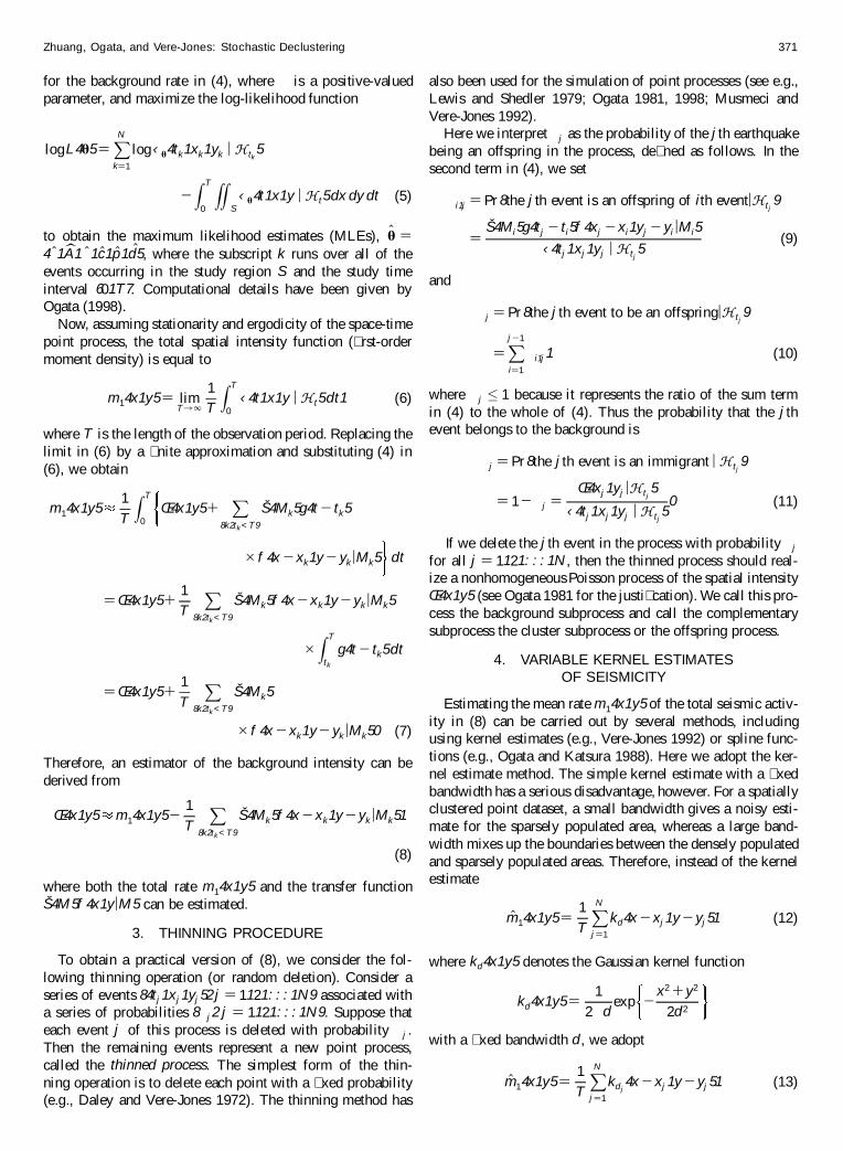
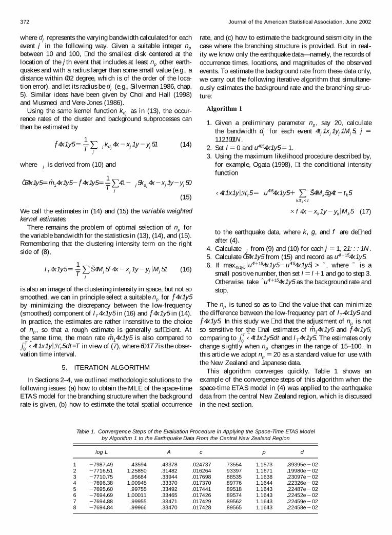
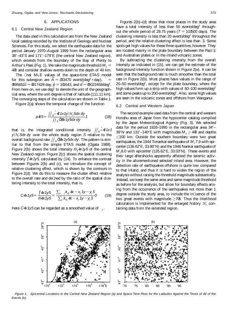
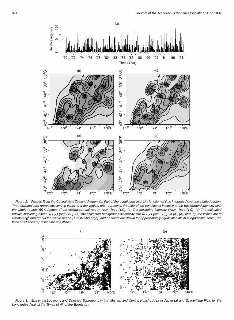
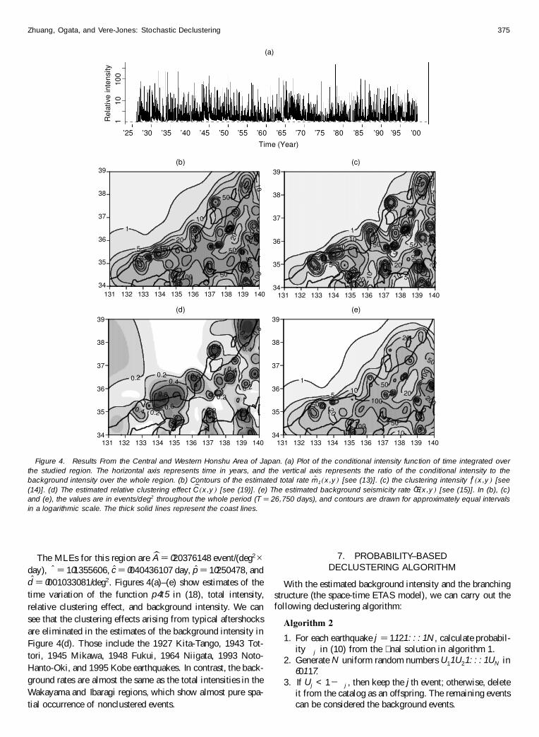
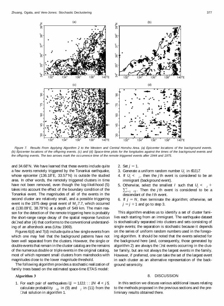
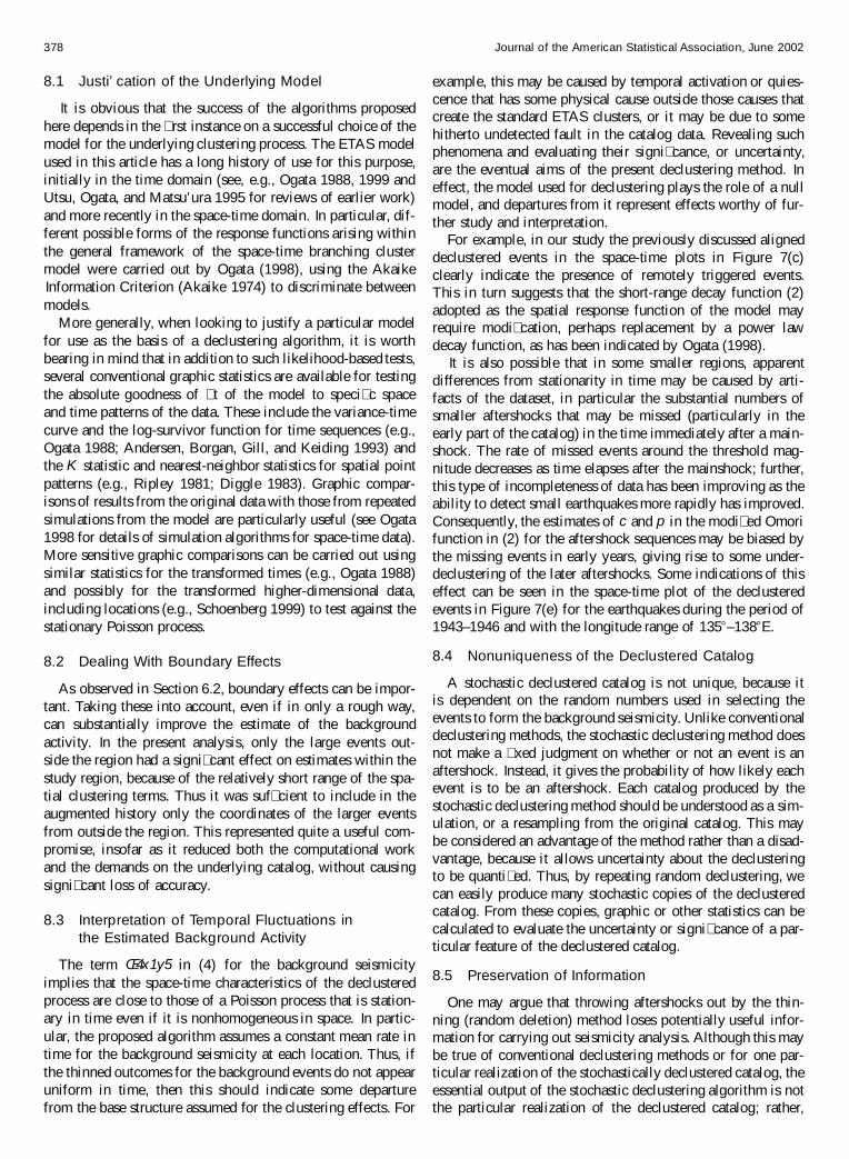