Author's Accepted Manuscript

Stochastic Efficiency Analysis with a Reliabil-ity Consideration

Guiwu Wei, Jian Chen, Jiamin Wang

PII: S0305-0483(14)00038-3DOI: http://dx.doi.org/10.1016/j.omega.2014.04.001Reference: OME1392

To appear in: Omega

Received date: 3 May 2012Revised date: 1 April 2014Accepted date: 3 April 2014

Cite this article as: Guiwu Wei, Jian Chen, Jiamin Wang, Stochastic EfficiencyAnalysis with a Reliability Consideration, Omega, http://dx.doi.org/10.1016/j.omega.2014.04.001

This is a PDF file of an unedited manuscript that has been accepted forpublication. As a service to our customers we are providing this early version ofthe manuscript. The manuscript will undergo copyediting, typesetting, andreview of the resulting galley proof before it is published in its final citable form.Please note that during the production process errors may be discovered whichcould affect the content, and all legal disclaimers that apply to the journalpertain.

www.elsevier.com/locate/omega

Stochastic Efficiency Analysis with a

Reliability Consideration

Guiwu Wei and Jian Chen

Department of Management Science and Engineering

School of Economics and Management, Tsinghua University, Beijing 100084, China

Jiamin Wang∗

College of Management, Long Island University Post, Brookville, NY 11548, USA

Revision 3

Abstract

Stochastic Data Envelopment Analysis (DEA) models have been introduced in the

literature to assess the performance of operating entities with random input and output

data. A stochastic DEA model with a reliability constraint is proposed in this study

that maximizes the lower bound of an entity’s efficiency score with some pre-selected

probability. We define the concept of stochastic efficiency and develop a solution pro-

cedure. The economic interpretations of the stochastic efficiency index are presented

when the inputs and outputs of each entity follow a multivariate joint normal distri-

bution.

Keywords: Data Envelopment Analysis; performance measurement; stochastic

efficiency analysis; chance constraint; value-at-risk

∗Corresponding author. Tel: 1(516)299-3914. Fax: 1(516)299-3917. Email address: jiamin.wang@liu.edu.

1

1 Introduction

Data Envelopment Analysis (DEA) is a non-parametric method used to evaluate the per-

formance of a set of operating entities called decision making units (DMUs) that consume

similar inputs and create similar outputs. Cooper, Seiford, and Tone [10] provided an in-

troduction of the various DEA models. Cook, Tone and Zhu [6] discussed the selection of

a DEA model. The reader is referred to Cook and Seiford [5] and Liu et al. [17, 18] for

extensive reviews of DEA’s development and applications.

Traditionally, the efficiency score of a DMU is defined as the ratio of the multiplier-

weighted sum of its outputs to the multiplier-weighted sum of its inputs. The constant

returns-to-scale DEA model, namely, the CCR DEA model [4], computes the efficiency indx

of a DMU, which is the maximum efficiency score in terms of the input and output multipliers.

Any DMU with an efficiency index of one is rated as CCR efficient in the sense that it is

not dominated by any observations or their linear combinations. The efficiency index of an

inefficient DMU is less than one and reveals the proportional decrease necessary in its inputs

to reach the estimated efficiency frontier, which is spanned by the efficient units.

It is widely acknowledged that variability and uncertainty are associated with the input

and output data of a production process due to its inherent stochastic nature or specification

errors [1]. Land, Lovell and Thore [14] gave convincing examples in agriculture, manufac-

turing, product development, education, health care and military for which it is necessary

to incorporate stochastic variation of data in the concept of “efficiency”. As a consequence,

both multiplier and envelopment DEA models have been generalized to deal with stochastic

inputs and outputs. The concepts of dominance and efficiency are extended to the stochas-

tic domain in these models, where chance-constrained programming is applied to model the

production frontier defined with stochastic inputs and outputs.

Land, Lovell, and Thore [14] proposed a stochastic efficiency analysis formulation in en-

velopment form where a chance constraint is placed on every output category. In this study

we focus on stochastic DEA models in multiplier form as they explicitly take into account

the correlations among input and output data within every DMU, which are generally con-

2

sidered more important than dependencies among the observed DMUs but are ignored in

envelopment models.

Cooper, Huang, Lelas, Li, and Olesen [8, 9], Huang and Li [12, 13] and Li [16] devel-

oped joint stochastic efficiency analysis models where probabilistic efficiency dominance is

established via a joint chance constraint. No computational results have been reported in

the literature possibly due to the strong intractability of these models.

We next examine two multiplier form stochastic DEA models with a marginal chance

constraint on every DMU. The following “satisficing” DEA model was presented in Cooper,

Huang, and Li [7]:

π∗o = max

u,vP{

uT yo

vT xo≥ 1

}

s.t.

P{

uT yj

vT xj≤ 1

}≥ αj, j ∈ N,

u ≥ 0, v ≥ 0.

(1)

In the model, it is assumed that every unit in the set of DMUs, N = {1, 2, ..., n},consumes resources in m categories and creates products or services in s categories. P means

“Probability”, yj = (y1j, y2j, · · ·, ysj)T and xj = (x1j, x2j, · · ·, xmj)T represent, respectively,

the vectors of stochastic output and input values of DMU j ∈ N , while u ∈ Rs and v ∈ Rm

are non-negative virtual multipliers to be determined by solving the above model for DMU

o, which is the DMU under evaluation. Throughout this paper, it is assumed that yrj and

xij are continuous random variables for any r = 1, 2, ..., s and any i = 1, 2, ...,m. αj ∈ (0, 1)

is pre-selected and is the minimum probability required to fulfill the corresponding chance

constraint.

We note that model (1) is adapted from the traditional CCR DEA model (Charnes,

Cooper, and Rhode [4]) and falls in the class that Charnes and Cooper [3] refer to as “P-

models”. As Charnes and Cooper suggested, the objective of a “P-model” can be linked to

the concept of “satisficing” defined by Simon [22]. Along this perspective, the unity in the

objective function of model (1) can be interpreted as an aspiration level, while model (1)

maximizes the likelihood for the efficiency score of DMU o to achieve this aspiration level.

3

Assuming that the random outputs and inputs of each DMU j follow a multivariate

normal distribution with a mean vector (yTj , x

Tj )

T and a variance-covariance matrix Λj,

Olesen and Petersen [20] developed a model that optimizes the rate at which the mean input

vector for the DMU under evaluation has to decrease in order to achieve efficiency. The

original formulation presented by Olesen and Petersen [20] has a typo. The model after the

necessary correction is presented as follows:

θ∗o = maxu,v

uTyo + Φ−1(αo)√(uT ,−vT )Λo(uT ,−vT )T

s.t.

vTxo = 1,

uTyj − vTxj + Φ−1(αj)√

(uT ,−vT )Λj(uT ,−vT )T ≤ 0, j ∈ N,

u ≥ 0, v ≥ 0.

(2)

In the model, Φ() is the standard normal distribution function and Φ−1() its inverse.

As will be illuminated in the next section, the stochastic efficiency index π∗o given by

model (1) is not a radial measure. In contrast, model (2) returns a radial measure θ∗o and

reduces to the CCR DEA model when there is no variability in input and output data.

Consequently, (2) is a general model with CCR DEA model as a special case. However, our

subsequent analysis will show that model (2) does not necessarily return a correct stochastic

efficiency index. In this study, we propose a stochastic efficiency analysis model that corrects

this shortcoming of model (2) using the concept of aspiration level introduced in model (1).

We next analyze an example to motivate the study.

2 A Motivating Example

Under the assumption of joint normality model (1) can be rewritten as follows:

4

ϑ∗o = max

u,v,ϑϑ

s.t.

uTyo − vTxo − ϑ√(uT ,−vT )Λo(uT ,−vT )T ≥ 0,

uTyj − vTxj + Φ−1(αj)√

(uT ,−vT )Λj(uT ,−vT )T ≤ 0, j ∈ N,

u ≥ 0, v ≥ 0.

(3)

where π∗o = Φ(ϑ∗

o).

Models (2) and (3) are interpreted in this section using an example of three DMUs with

a single output and a single input that follow a joint normal probability distribution. As

shown in Olesen and Petersen [20], each chance constraint uTyj − vTxj

+Φ−1(αj)√(uT ,−vT )Λj(uT ,−vT )T ≤ 0 in these two models generates a supporting hy-

perplane to a confidence region of DMU j at some confidence level related to the chance

constraint probability level αj. Olesen and Petersen [20] further noted that the production

possibility set (PPS) is spanned by these confidence regions in the input output space. We

present the motivating example in Figure 1 and Figure 2 without discussing the mathemati-

cal details. The confidence region of DMU j in both figures is an ellipsoid denoted by Dj(αj)

j = 1, 2, 3, αj > 50%, with the mean input and output (xj, yj) of DMU j at the center,

where the size of the region is derived from the probability level αj used in the j+1th chance

constraint in model (3). The straight line in the two figures spanned by ellipsoid D1(α1) is

the production frontier.

The other ellipsoids in the figures are adjusted confidence regions for DMU 2, the DMU

under evaluation. These adjusted regions are denoted by D′2(q, β) with the mean output y2

and the contracted mean input qx2 from DMU 2 at the center, where q ∈ (0, 1] is a radial

contraction rate of the mean input vector x2 and β is a reliability level to be explained

in details in Section 3. As shown in that section, if q = 1, i.e., no radial contraction is

performed, then we have D′2(1, 1−α2)=D2(α2), the confidence region of inputs and outputs

derived from a chance constraint at the probability level α2. However, if q ∈ (0, 1), then the

shape of the region is changed accordingly, as illustrated in Figure 2.

In Figure 1 we illustrate the confidence regions used in models (2) and (3). The three

5

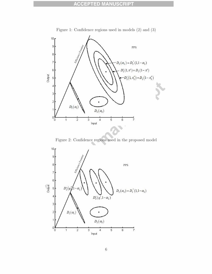
Figure 1: Confidence regions used in models (2) and (3)

PPS

Ef

ficie

ncy

Fron

tier

Figure 2: Confidence regions used in the proposed model

PPS

Ef

ficie

ncy

Fron

tier

6

concentric ellipsoids in Figure 1 are denoted byD2(α2) = D′2(1, 1−α2), D

′2(1, π

′) = D2(1−π′)

and D′2(1, π

∗2) = D2(1 − π∗

2), where π∗2 < π′ < 1 − α2. Note that D′

2(1, π∗2) is the largest

adjusted confidence region obtained by decreasing the reliability level β (with q = 1) that

is still a subset of the reference technology spanned by D1(α1). This implies that π∗2 is the

highest reliability level β such that the adjusted region D′2(1, β) overlaps with the production

frontier. It is evident that the stochastic efficiency index π∗o is not a radial measure.

On the contrary, the stochastic efficiency index θ∗o in model (2) is a radial measure.

Olesen and Petersen [20] interpreted θ∗o as the minimum proportional decrease in the random

inputs of DMU o subject to a requirement that every input output combination within the

confidence region Do(αo) after the transformation stays inside the estimated PPS. By this

interpretation, θ∗2 in our motivating example would be the minimum latent displacement

necessary to move ellipsoid D2(α2) in Figure 1 to overlap with the production frontier line.

It is easy to infer from Figure 1 that using model (2) and letting each confidence region

Dj(αj) shrink toward a point estimate will in the limit converge to the tradition CCR

efficiency analysis model based on the mean values of inputs and outputs from each DMU.

However, we note that the adjusted confidence region D′2(q, 1 − α2) presented in Figure

2 is in fact contracted when the mean input contraction rate q decreases. Unfortunately,

Olesen and Petersen [20] ignored the fact that a contraction of the mean input vector of an

evaluated DMU will affect the shape of an adjusted confidence region. As a result, model

(2) does not return the correct stochastic efficiency index for an inefficient DMU unless the

inputs of that DMU are deterministic.

The model we are going to develop in this paper corrects this error by applying the concept

of an aspiration level. In model (1), the aspiration level is fixed and set by the decision maker.

But in our proposed model the aspiration level itself is a decision variable. In addition, a

reliability chance constraint is introduced. The chance constraints and the variable aspiration

level in the new model generate hyperplanes to support two types of confidence regions as

shown in Figure 2. Take β = 1−α2 as an example. The ellipsoidsDj(αj) j = 1, 2, 3 define the

PPS, while decreasing the aspiration level q reduces the deviation between the production

frontier and the input output combinations inside the ellipsoid D′2(q, 1− α2). q

∗2 is thus the

7

contraction rate of the mean input of DMU 2 for which the ellipsoid D′2(q

∗2, 1− α2) has one

and only one intersection point with the production frontier line.

In Figure 2 we illustrate the confidence regions used in model (4) proposed in this paper.

The three ellipsoids with centers lined up at the same output level are denoted by D2(α2) =

D′2(1, 1 − α2), D

′2(q

′, 1 − α2) and D′2(q

∗2, 1 − α2), where q∗2 < q′2 < 1 and q∗2 is the smallest

radial contraction rate q of the mean input from DMU 2 that keeps the confidence region

D′2(q, 1 − α2) as a subset of the reference technology spanned by D1(α1). Each of these

adjusted confidence regions D′2(q, 1 − α2) will be shown in Section 3 to be generated by a

chance constraint of DMU 2 with some probability level β = 1−α2, referred to as a reliability

level below.

As illustrated in Figure 2, combining the use of the concept of an aspiration level from

model (1) with the use of confidence regions in model (2) allows us to propose a model in

this paper that explores two different types of confidence regions. Firstly, all DMUs con-

tribute with the confidence regions at selected probability levels based on the non-contracted

mean input output vectors. As in model (2), the PPS is the convex cone spanned by these

confidence regions and enlarged by adding a certain orthant to comply with strong input

and output disposability. Hence, each of these confidence regions may potentially play an

active role in spanning the PPS. Secondly, we introduce a reliability confidence region, which

reflects the shape and size of a confidence region for the evaluated DMU after contraction

of the mean input vector with a factor q. Based on these two different sets of confidence

regions we define the stochastic CCR efficiency index q∗o , a radial measure, as the maximum

contraction rate q of the mean input vector for the evaluated DMU that is necessary to move

and transform the reliability confidence region D′o(q, β) until it either is not a proper subset

of the PPS (if β < 0.5) or is entirely outside the PPS (if β > 0.5).

The contributions of our study are two fold. First, the model proposed in this paper

bridges the existing models (1) and (2). Cooper, Huang and Li [7] did not interpret the

stochastic efficiency index π∗o they proposed. The motivating example in this section has

illustrated that under the joint normality assumption π∗o is the highest reliability level β

necessary for an adjusted confidence region D′o(1, β) to overlap with the production frontier

8

of the PPS spanned by non-adjusted confidence regions of all DMUs in consideration. Hence

using the two types of confidence regions discussed above we establish a uniform framework

to interpret the stochastic efficiency indices given by the three models under the multivariate

joint normality assumption. Second, this proposed model complements a model in Cooper,

Huang and Li [7] for characterizing behaviors of satisficing. Using a non-unity aspiration

level, Cooper, Huang and Li [7] developed a variant of model (1) that can be applied to

perform a trade-off analysis between optimizing and satisficing by setting the aspiration

level for a stochastically inefficient entity to reach. As will be illustrated in Section 5, the

model proposed in the current study can be employed to do a similar trade-off analysis by

selecting the minimum probability level to achieve some aspiration level.

The remainder of the paper is organized as follows. In the next section, we introduce the

model and provide an economic interpretation of the stochastic efficiency index. This devel-

opment is followed by a solution procedure proposed in Section 4 for arbitrary probability

distributions of input and output levels. An illustrative example is analyzed in Section 5.

Concluding remarks are made in the last section.

3 Stochastic Efficiency Analysis

We present the stochastic DEA model in this section. The production possibility set un-

derlying the model and the stochastic efficiency index for multivariate normally distributed

inputs and outputs are also interpreted.

3.1 Model

We start with model (1). As remarked in Cooper, Huang, and Li [7], the model is always

feasible. Let vector A =(α1, α2, ..., αn). The optimal objective function value π∗o is the prob-

ability for the efficiency score of DMU o to exceed unity with the optimal virtual multipliers.

Note π∗o ≤ 1 − αo. Cooper, Huang, and Li [7] thus defined DMU o to be stochastically

efficient (which we call CHL efficient below) if and only if π∗o = 1−αo. It is easy to see that

there exists at least one DMU j ∈ N with π∗j = 1− αj for a given vector A.

9

In model (1), unity is chosen as the aspiration level. Specifying the aspiration level as a

decision variable, we develop a stochastic DEA model below:

q∗o = maxq∈R,u,v

q

s.t.

P{

uT yo

vT xo≥ q

}≥ βo,

P{

uT yj

vT xj≤ 1

}≥ αj, j ∈ N ,

u ≥ 0, v ≥ 0.

(4)

Here βo is given and q is a decision variable. For any set of virtual multipliers, q is

the maximum value that bounds the multiplier weighted output-input ratio of DMU o from

below with a probability of at least βo. The model seeks virtual multipliers to maximize q,

which is equivalent to maximizing the aspiration level to be achieved with a probability of

βo or above. We hence call the first chance constraint in the model a reliability constraint

and βo the reliability level.

Since all constraints in model (4) are satisfied by q = 0, u = 0 and v > 0, the model is

always feasible with q∗o ≥ 0. Evidently, if the input and output values are constant for any

DMU j, model (4) reduces to the deterministic DEA model, namely the CCR DEA model.

We therefore call (4) the stochastic CCR DEA model.

Note that the reliability constraint can be rewritten as P{

vT xo

uT yo≤ 1

q

}≥ βo and

vT xo

uT yois a

loss function. We can therefore interpret 1qas the Value-at-Risk (VaR) at the confidence level

of βo and thus treat model (4) as a VaR minimization problem (Larsen, Mausser, Uryasev

[15]).

It is evident that the stochastic efficiency index q∗o may be sensitive to the threshold

probability levels βo and αj. Increasing βo or αj tightens the corresponding chance constraint.

Therefore, q∗o is non-increasing in the parameters βo and αj, ∀j. We note that q∗o may exceed

unity if βo < 1 − αo. To render the definition of the stochastic efficiency index consistent

with that of its deterministic counterpart, we require βo ≥ 1− αo.

Definition 1. Given A and βo, DMU o at the reliability level of βo is (i) stochastically CCR

efficient if and only if q∗o = 1; (ii) stochastically CCR inefficient if q∗o < 1; (iii) stochastically

10

pseudo-efficient if q∗o = maxj∈N

{q∗j} < 1.

By the above definition, a DMU is stochastically pseudo-efficient if it has the highest

stochastic efficiency index and none of the DMUs is stochastically efficient.

Cooper, Huang and Li [7] noted that chance constrained programming makes it possible to

interpret an inefficient DMU as a satisficing efficient unit with some probability of occurrence.

The reader is referred to [7] for insightful discussions of “satisficing” and “inefficiency”. We

note that the results of model (4) could be interpreted in a similar way. For instance, suppose

that DMU o is stochastically efficient, i.e., q∗o = 1, with a very low reliability level βo, which

implies a high risk of failing to achieve the aspiration level. A higher reliability level βo is

preferred in a less risky efficiency evaluation. But it would render q∗o < 1. DMU o could be

deemed as satisficing efficient (acceptably inefficient) if q∗o is not far below 1. In Section 5 an

example illustrates that a trade-off analysis between optimizing (inefficiency) and satisficing

can be made by changing the reliability level in model (4).

Unlike model (2), model (4) does not require any specific probability distributions. The

proposition below shows that model (2) is a special case of model (4) under joint normality.

Proposition 1. Given A and βo = 1−αo, q∗o = θ∗o is true if (y

Tj , x

Tj )

T follows a multivariate

normal distribution for any j ∈ N , and (i) q∗o = 1, or (ii) q∗o < 1 but the input vector of

DMU o is deterministic.

Proof. Under the joint normality assumption, each chance constraint on DMU j in model (2)

is equivalent to P{

uT yj

vT xj≤ 1

}≥ αj. Let q

∗o , u

∗ and v∗ be an optimal solution to model (4). If

q∗o = 1, then we have (u∗)Tyo − (v∗)Txo +Φ−1(αo)√[(u∗)T , (−v∗)T ]Λj[(u∗)T , (−v∗)T ]T = 0.

It is easy to verify that u∗/[(v∗)Txo] and v∗/[(v∗)Txo] is feasible to model (2) with the

objective function value of 1, which is the maximum value possible. q∗o = θ∗o = 1 hence

follows. Now we consider the case where xo = xo is deterministic. Let Λ′o be the variance-

covariance matrix of the output vector yo. (u∗)Tyo − q∗o(v

∗)Txo +Φ−1(αo)√

(u∗)TΛ′ou∗ = 0

implies that u∗/[(v∗)Txo] and v∗/[(v∗)Txo] is feasible to model (2) with the objective function

value θ = q∗o . Assume that there exists a feasible solution u′ and v′ to model (2) with an

objective function value θ′> θ. It follows that θ′, u′ and v′ is feasible to model (4), which

11

contradicts the knowledge that q∗o is optimal.

3.2 Stochastic CCR Efficiency Index

We now interpret the stochastic CCR efficiency index q∗o . Similar to Olesen and Petersen

[20], we assume in this sub-section that the outputs and inputs of each DMU j follow a

known s + m dimensional multivariate normal distribution with a mean vector (yTj , x

Tj )

T

and a variance-covariance matrix Λj of full rank. This assumption is adopted because close

form expressions of the chance constraints in model (4) may not exist or may make it hard to

interpret the stochastic efficiency index if inputs and outputs follow probability distributions

other than normality. As noted by Cooper, Huang, and Li [7], the selection of the normal

distribution is not so restrictive since normal approximation is readily acceptable in many

situations. We further require αj ≥ 50% for DMU j.

3.2.1 Production Possibility Set

Note that model (4) and model (2) have identical chance constraints on DMUs under the joint

normality assumption. The study in Olesen and Petersen [20] suggested that the production

possibility set (PPS) defined by these chance constraints is spanned by the confidence regions

for the DMUs in consideration. We next briefly summarize the relevant results. The reader

is advised to consult Olesen and Petersen [19, 20] for details.

Let cj = Φ−1(αj) for any j ∈ N . Denote by χ2(s+m) a random variable following the chi-

square distribution with s+m degrees of freedom. The confidence region at the confidence

level ϕj = P (χ2(s+m) ≤ c2j) is supported by the chance constraint on DMU j ∈ N :

Dj(αj) = {(yT ,xT )T ∈ Rs+m+ |[(y−yj)

T , (x−xj)T ]Λ−1

j [(y−yj)T , (x−xj)

T ]T ≤ c2j}, (5)

whereΛ−1j is the inverse of the variance-covariance matrixΛj. Note that a random realization

of (yTj , x

Tj )

T is located inside the region Dj(αj) with a probability of ϕj.

As Olesen and Petersen [19] demonstrated, random realizations of DMU j that fall within

the confidence regionDj(αj) are positioned inside the PPS if cj ≥ 0, or equivalently, αj ≥ 0.5.

Therefore, the PPS for model (4), denoted by Q(A), is the envelopment of n confidence

12

regions Dj(αj), ∀j ∈ N . It follows that Q(A) = {(yT ,xT )T ∈ Rs+m+ |∃(yT

j , xTj )

T ∈ Dj(αj)

and λj ≥ 0, j ∈ N such that∑j∈N

λjxj ≤ x and∑j∈N

λjyj ≥ y}.

Denote by P(A) the set of feasible virtual multipliers under vectorA. It can be formulated

as

P(A) = {(uT ,−vT )T ∈ Rs+m|u ≥ 0, v ≥ 0 and P (uT yj−vT xj ≤ 0) ≥ αj, ∀j ∈ N}. (6)

Transforming the chance constraints in Eq. (6) into deterministic equivalent constraints,

we have

P(A) = {(uT ,−vT )T ∈ Rs+m|u ≥ 0,v ≥ 0

and uTyj−vTxj + Φ−1(αj)√

(uT ,−vT )Λj(uT ,−vT )T ≤ 0, ∀j ∈ N}.

Since αj ≥ 50%, uTyj−vTxj + Φ−1(αj)√(uT ,−vT )Λj(uT ,−vT )T is a convex function. It

follows that P(A) is in general a convex cone.

Theorem 5 in Olesen and Petersen [19] suggests that Q(A) presented in terms of P(A)

is given by

Q(A) = {(yT ,xT )T ∈ Rs+m+ |∀(uT ,−vT )T ∈ P(A) : uTy − vTx ≤ 0}. (7)

As a consequence, the production frontier for Q(A) can be presented as

Eff Q(A) = {(yT ,xT )T ∈ Rs+m+ |∃(uT ,−vT )T ∈ P(A) : uTy − vTx = 0}. (8)

3.2.2 Economic Interpretation

The stochastic CCR efficiency index given by model (4) is next interpreted. In a way similar

to derive Eq. (5), we claim that the reliability constraint defines a supporting hyperplane

to the following confidence region, which is called a reliability confidence region, at the

confidence level P [χ2(s+m) ≤ (Φ−1(βo))

2] for DMU o:

D′o(q, βo) = {(yT ,xT )T ∈ Rs+m

+ |[(y−yo)T , (x−qxo)

T ]Λ−1o [(y−yo)

T , (x−qxo)T ]T ≤ (Φ−1(βo))

2},(9)

13

where Λo = BΛoB and B = [bgh] is a (s+m)× (s+m) matrix with bgh = 0 if g �= h, bgg = 1

if g ≤ s and bgg = q otherwise. Note that D′o(q, βo) is a confidence region rendered after the

mean input vector of DMU o changes proportionally by q.

Given q, let V (q, βo) = {(uT ,−vT )T ∈ Rs+m|u ≥ 0, v ≥ 0 and P (uT yo−qvT xo ≥ 0) =

βo}, i.e., uTyo−qvTxo − Φ−1(βo)√(uT ,−qvT )Λo(uT ,−qvT )T = 0 holds for every vector

(uT ,−vT )T in V (q, βo). We consider 1− αo ≤ βo < 50% and αo, βo ≥ 50% separately.

Suppose 1 − αo ≤ βo < 50%. Given a vector (uT ,−vT )T ∈ V (q, βo), we have uTyo −qvTxo ≤ 0 as Φ−1(βo) < 0. Applying Corollary 1 in Olesen and Petersen [19], uTy − vTx ≤ 0

follows at any realization (yT ,xT )T ∈ D′o(q, βo). As will be shown later in Corollary 1, the

reliability constraint is binding at optimality. It implies that a vector (uT ,−vT )T in V (q∗o ,

βo) ∩ P(A) (the intersection of the two sets is not empty as the model is always feasible)

must be optimal. By Eqs. (7) and (8), we realize that the reliability confidence region

D′o(q

∗o , βo) is positioned inside the PPS Q(A). Since q∗o is the maximum objective function

value, D′o(q

∗o , βo) shall overlap with the production frontier Eff Q(A), that is, there exist

a realization (yT ,xT )T ∈ D′o(q

∗o , βo) and (uT ,−vT )T ∈ P(A) such that uTy − vTx = 0.

Note thatD′o(1, βo) is the original reliability confidence region andD′

o(q∗o , βo) the one after

every input of DMU o contracts by the rate q∗o . It now becomes clear that the stochastic

CCR efficiency index q∗o at the reliability level of βo measures the deviation between the

production frontier and the reliability confidence region D′o(1, βo). We can interpret q∗o as

follows.

• DMU o is stochastically CCR efficient if q∗o = 1, which implies that the reliability

confidence region D′o(1, βo) overlaps with the production frontier Eff Q(A). In other

words, there exists some random realization (yT ,xT )T ∈ D′o(1, βo) that lies on the

production frontier. As P [χ2(s+m) ≤ (Φ−1(βo))

2] ≤ ϕo, we know that D′o(1, βo) is a

subset of Do(αo). Note that the PPS Q(A) spans confidence regions Dj(αj) ∀j. It

follows that a necessary condition for q∗o = 1 is that confidence regions D′o(1, βo) and

Do(αo) coincide, i.e., βo + αo = 1.

• q∗o < 1 means no random realization in the reliability confidence region D′o(1, βo) is

14

efficient. q∗o is the maximum rate q of proportional decrease in the inputs of DMU o

before some input-output combination within D′o(q, βo) becomes efficient. The index

introduces a target reliability confidence region, D′o(q

∗o , βo), which overlaps with the

production frontier.

Now we consider αo ≥ 50% and βo ≥ 50%. In a way similar to the analysis for the

above case, we conclude that uTy − vTx ≥ 0 holds at any realization (yT ,xT )T ∈ D′o(q

∗o , βo)

for a multiplier vector (uT ,−vT )T ∈ V (q∗o , βo) ∩ P(A). As a result, the target reliability

confidence region D′o(q

∗o , βo) is positioned outside the PPS Q(A) with some realization on

the production frontier. q∗o is always less than unity and can be regarded as the maximum

rate q to decrease the mean input vector of DMU o until no input-output combination within

D′o(q, βo) is inefficient.

In summary, the stochastic CCR efficiency index q∗o is the maximum contraction rate q

of the input vector for DMU o that is necessary to move the reliability confidence region

D′o(q, βo) until (i) it is not a proper subset of the PPS if 1 − αo ≤ βo < 50% or (ii) it is

entirely outside the PPS if βo ≥ 50%.

Since Φ−1(50%) = 0, the confidence region Dj(50%) of DMU j reduces to a single point

(yTj , x

Tj )

T . Note that (yTo , x

To )

T is also the reliability confidence region D′o(1, 50%). It is

easy to see that q∗o coincides with the DMU’s deterministic CCR efficiency index (under the

assumption of no variability) when αj = 50% for any j ∈ N and βo = 50%. Hence the

deterministic and stochastic CCR efficiency indices can be interpreted similarly. But the

latter is concerned with a set of input-output combinations of the DMU under evaluation

instead of a single observation. Because q∗o is non-increasing as βo or αj increases, the

deterministic CCR efficiency index of a DMU o is no less than its stochastic counterpart q∗o

when αj > 50% ∀j ∈ N and βo > 50%.

Olesen and Petersen [20] interpreted θ∗o as the maximum reduction rate in the mean

inputs necessary for the confidence region Do(αo) to overlap with the estimated production

frontier. However, we note that the variance-covariance matrix for the inputs and outputs

of DMU o shall change accordingly as the mean inputs are displaced. Because the authors

ignore this change in modeling, their analysis would not identify the true target reliability

15

confidence region on the production frontier for an inefficient DMU and a correct stochastic

efficiency index is returned by model (2) only when the inefficient DMU’s input vector is

deterministic.

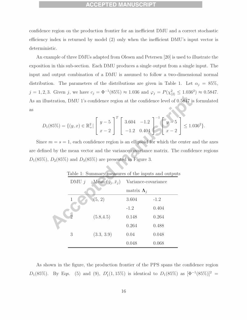
An example of three DMUs adapted from Olesen and Petersen [20] is used to illustrate the

exposition in this sub-section. Each DMU produces a single output from a single input. The

input and output combination of a DMU is assumed to follow a two-dimensional normal

distribution. The parameters of the distributions are given in Table 1. Let αj = 85%,

j = 1, 2, 3. Given j, we have cj = Φ−1(85%) ≈ 1.036 and ϕj = P (χ2(2) ≤ 1.0362) ≈ 0.5847.

As an illustration, DMU 1’s confidence region at the confidence level of 0.5847 is formulated

as

D1(85%) = {(y, x) ∈ R2+|

⎡⎣ y − 5

x− 2

⎤⎦T ⎡⎣ 3.604 −1.2

−1.2 0.404

⎤⎦

−1 ⎡⎣ y − 5

x− 2

⎤⎦ ≤ 1.0362}.

Since m = s = 1, each confidence region is an ellipsoid for which the center and the axes

are defined by the mean vector and the variance-covariance matrix. The confidence regions

D1(85%), D2(85%) and D3(85%) are presented in Figure 3.

Table 1: Summary measures of the inputs and outputs

DMU j Mean (yj, xj) Variance-covariance

matrix Λj

1 (5, 2) 3.604 -1.2

-1.2 0.404

2 (5.8,4.5) 0.148 0.264

0.264 0.488

3 (3.3, 3.9) 0.04 0.048

0.048 0.068

As shown in the figure, the production frontier of the PPS spans the confidence region

D1(85%). By Eqs. (5) and (9), D′1(1, 15%) is identical to D1(85%) as [Φ−1(85%)]2 =

16

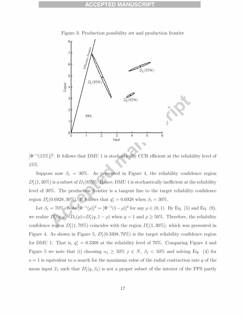
Figure 3: Production possibility set and production frontier

Ef

ficie

ncy

Fron

tier

PPS

[Φ−1(15%)]2. It follows that DMU 1 is stochastically CCR efficient at the reliability level of

15%.

Suppose now β1 = 30%. As presented in Figure 4, the reliability confidence region

D′1(1, 30%) is a subset ofD1(85%). Hence, DMU 1 is stochastically inefficient at the reliability

level of 30%. The production frontier is a tangent line to the target reliability confidence

region D′1(0.6928, 30%). It follows that q∗1 = 0.6928 when β1 = 30%.

Let β1 = 70%. Note [Φ−1(ρ)]2 = [Φ−1(1−ρ)]2 for any ρ ∈ (0, 1). By Eq. (5) and Eq. (9),

we realize D′1(q, ρ)=D1(ρ)=D′

1(q, 1− ρ) when q = 1 and ρ ≥ 50%. Therefore, the reliability

confidence region D′1(1, 70%) coincides with the region D′

1(1, 30%), which was presented in

Figure 4. As shown in Figure 5, D′1(0.3308, 70%) is the target reliability confidence region

for DMU 1. That is, q∗1 = 0.3308 at the reliability level of 70%. Comparing Figure 4 and

Figure 5 we note that (i) choosing αj ≥ 50% j ∈ N , β1 < 50% and solving Eq. (4) for

o = 1 is equivalent to a search for the maximum value of the radial contraction rate q of the

mean input x1 such that D′1(q, β1) is not a proper subset of the interior of the PPS partly

17

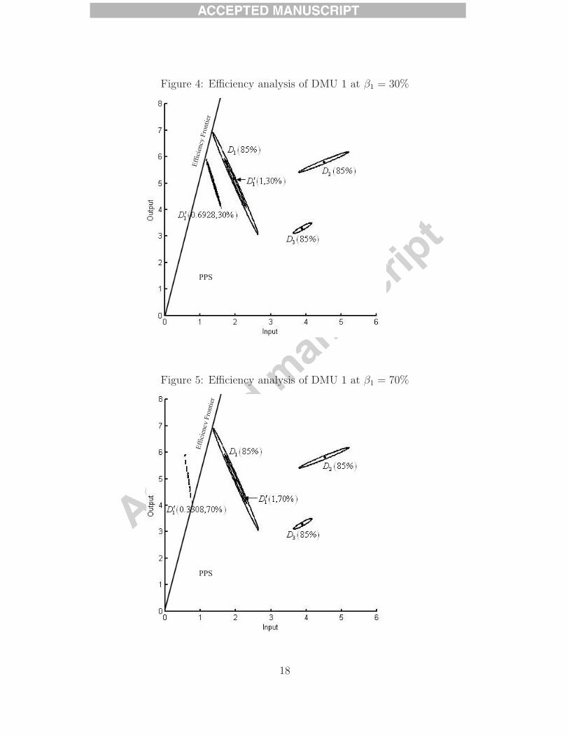
Figure 4: Efficiency analysis of DMU 1 at β1 = 30%

Ef

ficie

ncy

Fron

tier

PPS

Figure 5: Efficiency analysis of DMU 1 at β1 = 70%

Ef

ficie

ncy

Fron

tier

PPS

18

spanned by the confidence regions Dj(αj) for DMU j = 1, 2, 3; (ii) choosing αj ≥ 50% j ∈ N ,

β1 > 50% and solving Eq. (4) for o = 1 is equivalent to a search for the maximum value of

the radial contraction rate q of the mean input x1 such that the intersection of D′1(q, β1) and

the interior of the PPS partly spanned by the confidence regions Dj(αj) for DMU j = 1, 2, 3

is empty.

4 Solution Approach

We note that model (4) is difficult to solve directly due to its strong nonlinearity caused by

the decision variable q appearing in the reliability constraint as well as non-convexity. In

this section, we develop a solution procedure for model (4) by solving a series of models in

a form similar to (1), for which the deterministic equivalent formulation is relatively easier

to solve at least approximately.

The next result is useful to our ensuing exposition.

Proposition 2. Suppose that u′ and v′ are feasible multiplier vectors to the constraints

of model (4) other than the reliability constraint. Let q′ = max q subject to the reliability

constraint with u = u′ and v = v′. It follows that P{

(u′)T yo

(v′)T xo≥ q′

}= βo always holds.

Proof. Note that there exists at least one element in v′ that is not zero. Since yro and

xio are continuous random variables, P{

(u′)T yo

(v′)T xo≥ q

}in terms of q can be interpreted as a

continuous mapping into (0, 1). By the Intermediate Value Theorem [11], there exists some

value q′ such that P{

(u′)T yo

(v′)T xo≥ q′

}= βo. It is easy to verify that q′ = max q subject to the

reliability constraint.

The corollary below is trivial to prove.

Corollary 1. Let q∗o, u∗ and v∗ be optimal to model (4). It follows that P

{(u∗)T yo

(v∗)T xo≥ q∗o

}=

βo holds.

We now introduce the following programming problem with a given parameter η:

19

γ∗o(η) = max

u,vP{

uT yo

vT xo≥ η

}

s.t.

P{

uT yj

vT xj≤ 1

}≥ αj, j ∈ N ,

u ≥ 0, v ≥ 0.

(10)

The optimality condition of model (4) is presented below.

Theorem 1. γ∗o(q

∗o) = βo is the sufficient and necessary optimality condition for model (4).

Proof. We first show that the optimality condition is necessary. Let u∗, v∗ and q∗o be optimal

to model (4). It follows that u∗ and v∗ are feasible to model (10) for any η and γ∗o(q

∗o) ≥

βo. Suppose that for model (10) the optimal multipliers u′ and v′ are such that γ∗o(q

∗o) =

P{

(u′)T yo

(v′)T xo≥ q∗o

}> βo. It is easy to see that q = q∗o , u = u′ and v = v′ would be feasible to

model (4), which contradicts Proposition 2.

Next we show that the optimality condition is sufficient. Assume that γ∗o(q) = βo holds.

Suppose that u∗, v∗ and q∗o is the optimal solution to model (4) with q∗o > q. By Corollary

1, P{

(u∗)T yo

(v∗)T xo≥ q

}> βo and hence γ∗

o(q) > βo, which contradicts our assumption.

A solution procedure is developed to solve the optimality condition γ∗o(q

∗o) = βo.

Algorithm: Solving model (4)

Step 1 Let k = 1 and η(1) be sufficiently small.

Step 2 Solve model (10) with η = η(k). Denote by u(k) and v(k) the vectors of optimal

multipliers. We require that not all elements in u(k) are zero when k = 1.

Step 3 If γ∗o(η

(k)) − βo < δ (a pre-selected tolerance), then stop and return η(k) as q∗o .

Otherwise, let η(k+1) be the value such that P{

(u(k))T yo

(v(k))T xo≥ η(k+1)

}= βo, increase k to

k + 1 and go to Step 2.

The initial value of η should be chosen such that γ∗o(η

(1)) is 1 or close to 1. We can set

η(1) = 0 if inputs and outputs are all positive random variables. At the kth iteration of the

20

algorithm, the sub-problem (10) is solved for γ∗o(η

(k)). The optimal multipliers obtained are

then used to generate η(k+1). This process repeats until γ∗o(η

(k)) and βo become sufficiently

close.

The algorithm yields two sequences of numbers {η(k)} and {γ∗o(η

(k))}. The next proposi-tion characterizes the sequence {η(k)}.

Proposition 3. Iteration sequence {η(k)} is monotone increasing in k.

Proof. Note that γ∗o(η

(1)) is sufficiently close to 1. Since P{

(u(1))T yo

(v(1))T xo≥ η(2)

}= βo < 1, we

have η(1) < η(2). Suppose that the algorithm does not terminate at the kth iteration. Since

u(k) and v(k) are feasible to model (10), we have γ∗o(η

(k)) > βo + δ, P{

(u(k))T yo

(v(k))T xo≥ η(k+1)

}=

βo ≤ γ∗o(η

(k+1)). Hence, η(k) < η(k+1) unless γ∗o(η

(k)) − βo < δ and therefore the sequence

stops.

The next corollary is natural.

Corollary 2. Iteration sequence {γ∗o(η

(k))} is monotone decreasing in k.

According to the Monotone Convergence Principle [11], iteration sequence {γ∗o(η

(k))}converges to βo.

Now we consider a special case where the inputs and outputs of some DMUs are all

deterministic. Let J be the set of all such DMUs. The chance constraint in model (10) on

any DMU j ∈ J changes touTyj

vTxj≤ 1 or uTyj − vTxj ≤ 0, where again yj and xj denote

deterministic output and input vectors. If o /∈ J , then the algorithm presented above is still

applicable. Otherwise, the following single problem is solved for the efficiency index q∗o :

q∗o = maxu,v

uTyo

vTxo

s.t.

P{

uT yj

vT xj≤ 1

}≥ αj, j /∈ J,

uTyj

vTxj≤ 1, j ∈ J,

u ≥ 0, v ≥ 0.

21

By the Charnes-Cooper transformation of linear fractional programming problems [2], the

above model can be rewritten as

q∗o = maxu,v

uTyo

s.t.

vTxo = 1,

P{

uT yj

vT xj≤ 1

}≥ αj, j /∈ J,

uTyj − vTxj ≤ 0, j ∈ J,

u ≥ 0, v ≥ 0.

(11)

The iterative algorithm presented earlier in this section, which we call Algorithm 1 can

be applied here by replacing model (10) with model (11).

We note that the algorithms developed in this section are applicable to general prob-

ability distributions. The sub-problem (10) can be solved in a way similar to model (1).

Cooper, Huang, and Li [7] derived deterministic quadratic programs equivalent to model

(1), respectively, under two assumptions:

• Stochastic outputs and inputs are related only through a single normally distributed

factor.

• Input and output values are random variables following a multivariate normal distri-

bution.

In the next section, we will illustrate how to derive a deterministic equivalent problem for

model (10). We recommend that the reader refer to Cooper, Huang, and Li [7] for details.

5 An Illustrative Example

We now evaluate the performance of a subset of the selected gas stations studied by Suyoshi

[23] to illustrate model (4) and the algorithms developed in the previous section. In the

computational studies, the linear problems are solved in Lindo What’sBest! 10.0, an Ex-

cel spreadsheet add-in for mathematical programming, while Algorithms 1 is coded using

Microsoft VBA (Visual Basic for Applications).

22

Sueyoshi [23] used a data set generated in summer 1998 to predict future operational

performance of sixty selected gas stations in Tokyo, Japan. The three inputs in the data set

are the number of employees; the space size of a gas station; and the monthly operational

cost. The input values were observed in summer 1998 and assumed to be deterministic.

The two outputs chosen are the sales of gasoline and petrol to be realized in winter 1998.

The output levels were unknown at the time and a manager in a Japanese petroleum firm

was asked to provide the most likely estimate, the optimistic estimate and the pessimistic

estimate for either output of each gas station. Under the assumption that a random output

level is independent and follows a particular beta distribution used in PERT/CPM Sueyoshi

[23] applied these estimates to approximate the means and variances of the outputs. (We

note that Eq. (18) in [23] has typos. It should read b2rj = [(OPrj −PErj)/6]2.) Furthermore,

the author adopted the single factor symmetric disturbance assumption, i.e., the component

of any output determined solely by a single underlying random factor ξ is formulated as

yrj = yrj + brjξ,

for j = 1, 2, ..., n and r = 1, 2, ..., s, where ξ follows the standard normal distribution. Note

that yrj is the expected value of yrj, while brj is the standard deviation. We would like

to point out that the assumptions of an independent PERT-beta distribution and a single

factor symmetric distribution are inconsistent, while the author did not motivate or justify

these assumptions. Despite these problematic assumptions we choose the data set presented

in [23] as an illustrative example because there are very few applications of stochastic DEA

models available in the literature.

In the computational study, we run models (1) and (4) on this data set. Only the twenty

gas stations classified as “large” (1st to 20th DMUs in Table 1 and Table 2 of [23]) are

assessed.

Let yj = (y1j, y2j, ..., ysj)T and bj = (b1j, b2j, ..., bsj)

T . xj = (x1j, x2j, ..., xmj) denotes the

vector of deterministic input values for DMU j.

Proceeding in a way analogous to Cooper, Huang and Li ([7]), we can obtain a linear

programming model equivalent to model (1) under the single factor symmetric disturbance

23

assumption:

κ∗o = max

u,vuTyo − vTxo

s.t.

uTbo = 1,

uTyj − vTxj + Φ−1(αj)uTbj ≤ 0, j ∈ N ,

u ≥ 0, v ≥ 0.

Similarly, a linear programming model equivalent to model (10) can be derived:

ω∗o(η) = max

u,vuTyo − ηvTxo

s.t.

uTbo = 1,

uTyj − vTxj + Φ−1(αj)uTbj ≤ 0, j ∈ N ,

u ≥ 0, v ≥ 0.

(12)

Remark 1. Note π∗o = Φ(κ∗

o) and γ∗o(η) = Φ(ω∗

o(η)). When Algorithm 1 is applied, model

(12) is solved at the kth iteration with η = η(k), while the optimal virtual multiplier vectors,

denoted by u(k) and v(k) are used to compute η(k+1) as

η(k+1) =Φ−1(β) + (u(k))Tyo

(v(k))Txo

.

Remark 2. Since model (1) was solved as a linear program and Algorithm 1 iteratively solved

a series of linear programs, the true values of π∗o and q∗o were returned in this computational

study for every DMU o.

The computational results of model (1) are presented in Table 2 with α = αj = 95%,

90%, 80%, ∀j ∈ N . It is easy to see that for any of these values of α stations 6, 15, 17, and

20 are deemed CHL efficient.

24

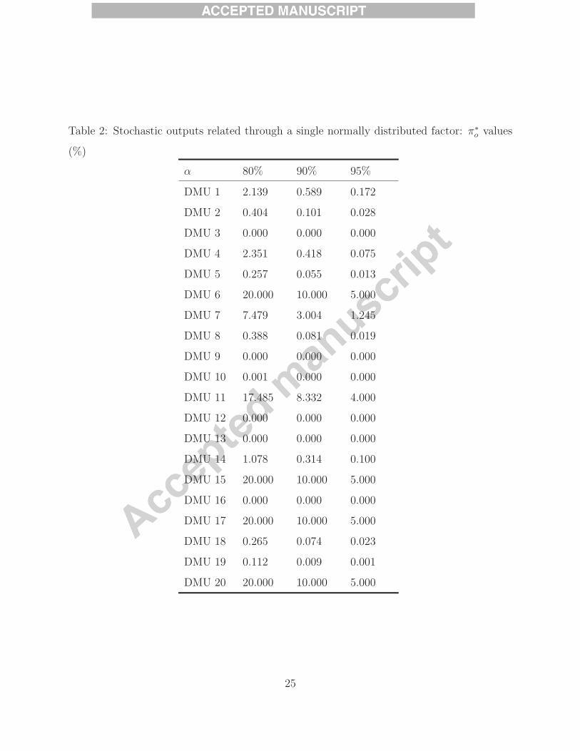
Table 2: Stochastic outputs related through a single normally distributed factor: π∗o values

(%)

α 80% 90% 95%

DMU 1 2.139 0.589 0.172

DMU 2 0.404 0.101 0.028

DMU 3 0.000 0.000 0.000

DMU 4 2.351 0.418 0.075

DMU 5 0.257 0.055 0.013

DMU 6 20.000 10.000 5.000

DMU 7 7.479 3.004 1.245

DMU 8 0.388 0.081 0.019

DMU 9 0.000 0.000 0.000

DMU 10 0.001 0.000 0.000

DMU 11 17.485 8.332 4.000

DMU 12 0.000 0.000 0.000

DMU 13 0.000 0.000 0.000

DMU 14 1.078 0.314 0.100

DMU 15 20.000 10.000 5.000

DMU 16 0.000 0.000 0.000

DMU 17 20.000 10.000 5.000

DMU 18 0.265 0.074 0.023

DMU 19 0.112 0.009 0.001

DMU 20 20.000 10.000 5.000

25

Applying Algorithm 1, we assess the efficiency of each gas station by solving a series

of linear programming problems. Table 3 gives q∗o of the twenty “large” gas stations with

combinations between α = αj = 95%, 90%, 80%, ∀j ∈ N and β = βo = 1 − α, 50%, and

α. It is obvious that q∗o decreases with α and β. We note that all CHL efficient units are

stochastically CCR efficient when β = 1 − α. If β = α or β = 50%, none of the units is

stochastically CCR efficient, but station 20 appears to be stochastically pseudo-efficient.

Next the same data set is used to demonstrate the application of model (4) to perform a

trade-off analysis between optimizing and satisficing. Applying the model, the manager of

each gas station o seeks the highest aspiration level to be achieved with a chosen probability

βo. In light of the economic interpretation of the stochastic CCR efficiency index, this is

equivalent to finding the maximum radial input contraction rate necessary for DMU o to

become stochastically efficient with a reliability level βo.

Take station 15 as an instance. Our computational results presented in Table 3 suggest

q∗15 = 1.0 when β15 = 10% and α = 90%. That is, station 15 is stochastically CCR efficient

at the reliability level of 10%. Following our analysis in Section 3, we infer that the reliability

confidence region D′15(1.0, 10%) shall be large so that some realizations are on the production

frontier, which implies that the risk of failing to achieve the aspiration level of 1.0 is high.

The manager of the gas station may prefer a higher reliability level β15 and therefore a smaller

reliability confidence region in order to perform a less risky efficiency evaluation. Increasing

β15 renders q∗15 < 1 and requires that the inputs of the gas station be cut to q∗15 × 100% of

the original levels so as to remain efficient and thus stay in business. Recall that given αj

∀j, q∗15 is non-increasing in β15. As β15 increases, the performance of the gas station should

improve, if feasible, in order to generate the desired outputs using less inputs.

Given α = αj = 90% ∀j, we obtain q∗15 = 0.9732 at β15 = 30% and q∗15 = 0.8871 at

β15 = 95%. An input (cost) reduction rate of 0.8871 with a reliability level of 95% seems

preferred. However, our analysis in Section 3 indicates that the target reliability confidence

region D′15(0.8871, 95%) is outside the production possibility set. The manager of station 15

as a satisficer may thus argue that it is too costly or technically challenging to make changes

to the process necessary to be efficient while cutting the inputs to 88.71% of the current

26

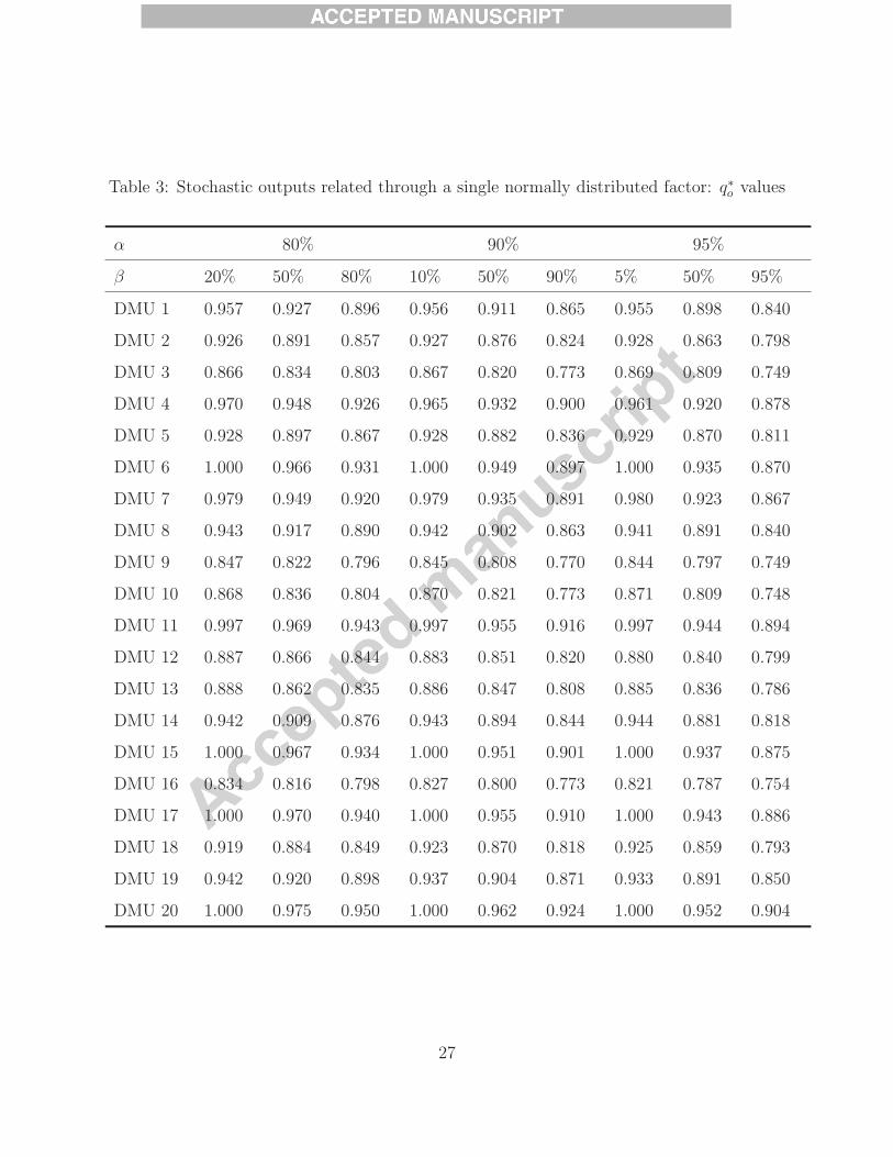
Table 3: Stochastic outputs related through a single normally distributed factor: q∗o values

α 80% 90% 95%

β 20% 50% 80% 10% 50% 90% 5% 50% 95%

DMU 1 0.957 0.927 0.896 0.956 0.911 0.865 0.955 0.898 0.840

DMU 2 0.926 0.891 0.857 0.927 0.876 0.824 0.928 0.863 0.798

DMU 3 0.866 0.834 0.803 0.867 0.820 0.773 0.869 0.809 0.749

DMU 4 0.970 0.948 0.926 0.965 0.932 0.900 0.961 0.920 0.878

DMU 5 0.928 0.897 0.867 0.928 0.882 0.836 0.929 0.870 0.811

DMU 6 1.000 0.966 0.931 1.000 0.949 0.897 1.000 0.935 0.870

DMU 7 0.979 0.949 0.920 0.979 0.935 0.891 0.980 0.923 0.867

DMU 8 0.943 0.917 0.890 0.942 0.902 0.863 0.941 0.891 0.840

DMU 9 0.847 0.822 0.796 0.845 0.808 0.770 0.844 0.797 0.749

DMU 10 0.868 0.836 0.804 0.870 0.821 0.773 0.871 0.809 0.748

DMU 11 0.997 0.969 0.943 0.997 0.955 0.916 0.997 0.944 0.894

DMU 12 0.887 0.866 0.844 0.883 0.851 0.820 0.880 0.840 0.799

DMU 13 0.888 0.862 0.835 0.886 0.847 0.808 0.885 0.836 0.786

DMU 14 0.942 0.909 0.876 0.943 0.894 0.844 0.944 0.881 0.818

DMU 15 1.000 0.967 0.934 1.000 0.951 0.901 1.000 0.937 0.875

DMU 16 0.834 0.816 0.798 0.827 0.800 0.773 0.821 0.787 0.754

DMU 17 1.000 0.970 0.940 1.000 0.955 0.910 1.000 0.943 0.886

DMU 18 0.919 0.884 0.849 0.923 0.870 0.818 0.925 0.859 0.793

DMU 19 0.942 0.920 0.898 0.937 0.904 0.871 0.933 0.891 0.850

DMU 20 1.000 0.975 0.950 1.000 0.962 0.924 1.000 0.952 0.904

27

levels. Instead, the manager may be satisfided with reducing the inputs to 97.32% of the

current levels with a reliability of 30% if the necessary changes to the process are easy to

implement.

6 Concluding Remarks

It is critical to consider data uncertainty and variability when assessing the performance

of DMUs. A chance-constrained efficiency analysis model with a reliability constraint has

been proposed in this paper. This new model links the formulations developed by Olesen

and Petersen [20] and Cooper, Huang and Li [7], and can be applied to perform a trade-off

analysis between optimizing and satisficing.

For multivariate joint normal inputs and outputs the stochastic efficiency index intro-

duced in this study is shown to be a radial measure that can be interpreted in a way similar

to the deterministic CCR efficiency index. The chance constraints in the proposed model

support two types of confidence regions in the input-output space. Every DMU contributes

a confidence region with its non-contracted mean input and output vectors at the center.

These confidence regions span the production possibility set. The reliability constraint gen-

erates a hyperplane to support a reliability confidence region of the DMU under evaluation

based on the mean output vector and contracted mean input vector as well as the reliability

level chosen. The stochastic efficiency index is the maximum contraction rate such that

the reliability region is either not a proper subset of the production possibility set (if the

reliability level is less than 0.5) or completely out of the production possibility set (if the

reliability level is greater than 0.5).

In this study, we have suggested a solution method that determines the stochastic CCR

efficiency index for a DMU by generating and solving sub-problems iteratively. We realize

that this method cannot guarantee a global optimum in instances where the sub-problems

are not convex programs. This snag is common for stochastic DEA models [24]. The task

of developing a more effective algorithm is left for future research.

28

Acknowledgment

The authors would like to thank the anonymous referees for their insightful comments and

suggestions.

References

[1] M.E. Bruni, D. Conforti, P. Beraldi, E. Tundis, Probabilistically constrained models for

efficiency and dominance in DEA, International Journal of Production Economics 117

(2009) 219-228.

[2] A. Charnes, W.W. Cooper, Programming with linear fractional functions, Naval Re-

search Logistics 9 (1962) 181-185.

[3] A. Charnes, W.W. Cooper, Deterministic equivalents for optimizing and satisfying under

chance constraints, Operations Research 11 (1963) 18-39.

[4] A. Charnes, W.W. Cooper, E. Rhode, Measuring the efficiency of decision making units,

European Journal of Operational Research 2 (1978) 429-444.

[5] W.D. Cook, L.M. Seiford, Data envelopment analysis (DEA) – Thirty years on, Euro-

pean Journal of Operational Research 192 (2009), 1-17.

[6] W.D. Cook, K. Tone, J. Zhu, Data envelopment analysis: Prior to choosing a model,

Omega 44 (2014), 1-4.

[7] W.W. Cooper, Z. Huang, S. Li, Satisficing DEA model under chance constraints, Annals

of Operations Research 66 (1996) 279-295.

[8] W.W. Cooper, Z. Huang, V. Lelas, S. Li, O. Olesen, Chance constrained program-

ming formulations for stochastic characterizations of efficiency and dominance in DEA,

Journal of Productivity Analysis 9 (1998) 53-79.

29

[9] W.W. Cooper, Z. Huang, S. Li, Chance constrained DEA, in W.W. Cooper, L.M.

Seiford, J. Zhu (Eds.), Handbook on Data Envelopment Analysis, Kluwer, Boston, MA,

2004, pp. 229-264.

[10] W.W. Cooper, L.M. Seiford, K. Tone, Data Envelopment Analysis: A Comprehensive

Text with Models, Applications, References and DEA-Solver Software, Kluwer Aca-

demic Publisher, New York, NY, 1999.

[11] R. Godement, Analysis I: Convergence, Elementary Functions, Springer-Verlag, Berlin,

Germany, 1998.

[12] Z. Huang, S. Li, Dominance stochastic models in data envelopment analysis, European

Journal of Operational Research 95 (1996) 390-403.

[13] Z. Huang, S. Li, Stochastic DEA models with different types of input output distur-

bance. Journal of Productivity Analysis 15 (2001) 95-113.

[14] K.C. Land, C.A.K. Lovell, S. Thore, Chance-constrained data envelopment analysis,

Managerial and Decision Economics 14 (1993) 541-554.

[15] N. Larsen, H. Mausser, S. Uryasev, Algorithms for optimization of Value-at-risk, in

P.M. Padlos, V.K. Tsitsiringos (Ed.), Financial Engineering, E-commerce and Supply

Chain, Kluwer, Boston, MA, 2001, pp. 19-46.

[16] S. Li, Stochastic models and variable returns to scales in Data Envelopment Analysis,

European Journal of Operational Research 104 (1998) 532-548.

[17] J. S. Liu, L.Y.Y. Lu, W.M. Lu, B.J.Y. Lin, Data envelopment analysis 1978-2010: A

criterion-based literature survey, Omega 41 (2013) 3-15.

[18] J. S. Liu, L.Y.Y. Lu, W.M. Lu, B.J.Y. Lin, A survey of DEA applications, Omega 41

(2013) 893-902.

[19] O.B. Olesen, N.C. Petersen, Foundation of chance constrained Data Envelopment Anal-

ysis for Pareto-Koopmann efficient production possibility sets, Working paper (1993).

30

[20] O.B. Olesen, N.C. Petersen, Chance constrained efficiency evaluation, Management Sci-

ence 41 (1995) 442-457.

[21] B. Rich, Schaum’s Outline of Modern Elementary Algebra, McGraw-Hills, New York,

NY, 1973, pp. 303.

[22] H.A. Simon, Models of Man, Wiley, New York, NY, 1957, pp. 243-273.

[23] T. Sueyoshi, Stochastic DEA for restructure strategy: an application to a Japanese

petroleum company, Omega 28 (2000) 385-398.

[24] A. Udhayakumar, V. Charles, M. Kumar, Stochastic simulation based genetic algorithm

for chance constrained data envelopment analysis, Omega 39 (2011) 387-397.

31