Author's Accepted Manuscript

Stochastic lot sizing problem with controlla-ble processing times

Esra Koca, Hande Yaman, M. Selim Aktürk

PII: S0305-0483(14)00142-XDOI: http://dx.doi.org/10.1016/j.omega.2014.11.003Reference: OME1450

To appear in: Omega

Received date: 19 January 2014Accepted date: 6 November 2014

Cite this article as: Esra Koca, Hande Yaman, M. Selim Aktürk, Stochastic lotsizing problem with controllable processing times, Omega, http://dx.doi.org/10.1016/j.omega.2014.11.003

This is a PDF file of an unedited manuscript that has been accepted forpublication. As a service to our customers we are providing this early version ofthe manuscript. The manuscript will undergo copyediting, typesetting, andreview of the resulting galley proof before it is published in its final citable form.Please note that during the production process errors may be discovered whichcould affect the content, and all legal disclaimers that apply to the journalpertain.

www.elsevier.com/locate/omega

Stochastic Lot Sizing Problem with Controllable

Processing Times

Esra Koca, Hande Yaman and M. Selim Akturk

Department of Industrial Engineering, Bilkent University, Ankara 06800 Turkey

ekoca, hyaman, akturk@bilkent.edu.tr

Abstract

In this study, we consider the stochastic capacitated lot sizing problem with controllable

processing times where processing times can be reduced in return for extra compression cost.

We assume that the compression cost function is a convex function as it may reflect increasing

marginal costs of larger reductions and may be more appropriate when the resource life, en-

ergy consumption or carbon emission are taken into consideration. We consider this problem

under static uncertainty strategy and α service level constraints. We first introduce a nonlin-

ear mixed integer programming formulation of the problem, and use the recent advances in

second order cone programming to strengthen it and then solve by a commercial solver. Our

computational experiments show that taking the processing times as constant may lead to more

costly production plans, and the value of controllable processing times becomes more evident

for a stochastic environment with a limited capacity. Moreover, we observe that controllable

processing times increase the solution flexibility and provide a better solution in most of the

problem instances, although the largest improvements are obtained when setup costs are high

and the system has medium sized capacities.

Keywords: Stochastic lot sizing, Controllable processing times, Second order cone pro-

gramming

1

1 Introduction

In this paper, we consider the lot sizing problem with controllable processing times where demand

follows a stochastic process and processing times of jobs can be controlled in return for extra

cost (compression cost). Processing time of a job can be controlled (and reduced) by changing

the machine speed, allocating extra manpower, subcontracting, overloading, consuming additional

money or energy. Although these options are available in many real life production and inventory

systems, in the traditional studies on the lot sizing problem, processing times of jobs are assumed

as constant.

Since the seminal paper of Wagner and Whitin (1958), the lot sizing problem and its extensions

have been studied widely in the literature (see Karimi et al. (2003), Robinson et al. (2009) for a

detailed review on the variants of the lot sizing problem). In the classical lot sizing problem, it

is assumed that the demand of each period is known with certainty although this is not the case

for most of the production and inventory systems and approximating the demand precisely may be

very difficult. In the stochastic lot sizing problem, this assumption is relaxed but the probability

distribution of the demand is assumed as known.

As reducing processing time of a job is equivalent to increasing production capacity, sub-

contracting, overloading or capacity acquisition can be seen as special cases of the controllable

processing times. There are studies in the literature that consider the lot sizing problem with

subcontracting (or outsourcing) (Atamturk and Hochbaum (2001), Helber et al. (2013), Merzifon-

luoglu et al. (2007)) or capacity acquisition (or expansion) (Ahmed et al. (2003), Luss (1982),

Rajagopalan and Swaminathan (2001)). However, in all of these studies costs of these options are

assumed as linear or concave. This assumption makes it possible to extend the classical extreme

point or optimal solution properties for these cases. In our study, we assume that the compression

cost is a convex function of the compression amount.

Controllable processing times are well studied in the context of scheduling. Earlier studies on

this subject assume linear compression costs as adding nonlinear terms to the objective (total cost)

function may make the problem more difficult (Kayan and Akturk, 2005). However, as it is stated

in recent studies, reducing processing times gets harder (and more expensive) as the compression

amount increases in many applications (Kayan and Akturk (2005), Akturk et al. (2009)). For

example, by increasing machine speed, processing times can be reduced, but this also decreases

2

life of the tool and an additional tooling cost is incurred. Moreover, increasing the machine speed

may also increase the energy consumption of the facility. Another example is a transportation

system in which trucks may be overloaded or their speeds could be increased in return for extra cost

due to increasing fuel consumption or limiting the carbon emission. Thus, considering a convex

compression cost function is realistic since a convex function represents increasing marginal costs

and may limit higher usage of the resource due to environmental issues.

In our study, we consider the following convex compression cost function for period t: γt (kt) =

κt (kt)a/b where kt > 0 is the total compression amount in period t, κt ≥ 0 and a≥ b > 0, a,b∈ Z+.

Note that, for a > b and κt > 0, γt is strictly convex. This function can represent increasing

marginal cost of compressing processing times in larger amounts. Moreover, this function can

be related to a (convex) resource consumption function (Shabtay and Kaspi (2004), Shabtay and

Steiner (2007b)). Suppose that one additional unit of the resource costs κt and for compressing

the processing time by kt units, additional ka/bt units of resource should be allocated. Thus, in this

context, compression cost represents resource consumption cost and the resource may be a contin-

uous nonrenewable resource such as energy, fuel or catalyzer. With the recent advances in convex

programming techniques, many commercial solvers (like IBM ILOG CPLEX) can now solve sec-

ond order cone programs (SOCP). In this study, we make use of this technique and formulate the

problem as SOCP so that it can be solved by a commercial solver.

The contributions of this paper are threefold:

• To the best of our knowledge, this is the first study that considers the stochastic lot sizing

problem with controllable processing times. Although this option is applicable to many real

life systems, the processing times are assumed as constant in the existing literature on lot

sizing problems.

• The inclusion of a nonlinear compression cost function complicates the problem formulation

significantly. Therefore, we utilize the recent advances in second order cone programming

to alleviate this difficulty, so that the proposed conic formulations could be solved by a com-

mercial solver in a reasonable computation time instead of relying on a heuristic approach.

• Since assuming fixed processing times unnecessarily limits the solution flexibility, we con-

duct an extensive computational experiments to identify the situations where controlling the

3

processing times improves the overall production cost substantially.

The rest of the paper is organized as follows. In the next section, we briefly review the related

literature. In Section 3, we formulate the problem and in Section 4, we strengthen the formu-

lation using the second order conic strengthening. In Section 5, we present the results of our

computational experiments. We first compare alternative conic formulations presented in Section

5, afterwards we investigate the impact of controllable processing times on production costs. In

Section 6, conclusions and future research directions are discussed.

2 Literature Review

Here, we first review the studies on stochastic lot sizing problems. Silver (1978) suggests a heuris-

tic solution procedure for solving the stochastic lot sizing problem. Laserre et al. (1985) consider

the stochastic capacitated lot sizing problem with inventory bounds and chance constraints on in-

ventory. They show that solving this problem is equivalent to solving a deterministic lot sizing

problem. Bookbinder and Tan (1988) study the stochastic uncapacitated lot sizing problem with

α-service level constraints under three different strategies (static uncertainty, dynamic uncertainty

and static-dynamic uncertainty). Service level α represents the probability that inventory will not

be negative. In other words, it means that with probability α , the demand of any period will be

satisfied on time. Under the static uncertainty decision rule, which is the strategy that will be used

in our study, all the decisions (production and inventory decisions) are taken at the beginning of the

planning horizon (frozen schedule). The authors formulate the problem and show that their model

is equivalent to the deterministic problem by showing the correspondence between the terms of

these two formulations.

Service level constraints are mostly used in place of shortage or backlogging costs in the

stochastic lot sizing problems. Since shortages may lead to loss of customer goodwill or delays

on the other parts of the system, it may be hard to estimate the backlogging or shortage costs in

the real life production and inventory systems. Rather than considering the backlogging cost as a

part of the total cost function, a specified level of service (in terms of availability of stock) can be

assured by service level constraints and when the desired service level is high, backlogging costs

can be omitted. This situation makes the usage of service level constraints more popular in the real

4

life systems (Bookbinder and Tan (1988), Nahmias (1993), Chen and Krass (2001)). A detailed

investigation of different service level constraints can be found in Chen and Krass (2001).

Vargas (2009) studies (the uncapacitated version of) the problem of Bookbinder and Tan (1988)

but rather than using service level constraints he assumes that there is a penalty cost for back-

logging, the cost components are time varying and there is a fixed lead time. He develops a

stochastic dynamic programming algorithm, which is tractable when the demand follows a normal

distribution. Sox (1997) studies the uncapacitated lot sizing problem with random demand and

non-stationary costs. He assumes that the distribution of demand is known for each period and

considers the static-uncertainty model, but uses penalty costs instead of service level constraints.

He formulates the problem as an MIP with nonlinear objective (cost) function and develops an

algorithm that resembles the Wagner-Whitin algorithm.

In the static-dynamic uncertainty strategy of Bookbinder and Tan (1988), the replenishment

periods are determined first, and then replenishment amounts are decided at the beginning of these

periods. They also suggest a heuristic two-stage solution method for solving this problem. Tarım

and Kingsman (2004) consider the same problem and formulate it as MIP. Moreover, Ozen et al.

(2012) develop a non-polynomial dynamic programming algorithm to solve the same problem.

Recently, Tunc et al. (2014) reformulate the problem as MIP by using alternative decision variables

and Rossi et al. (2014) propose an MIP formulation based on the piecewise linear approximation

of the total cost function, for different variants of this problem.

In the dynamic uncertainty strategy, production decision for any period is made at the beginning

of that period. Dynamic and static-dynamic strategies are criticized due to the system nervousness

they cause; supply chain coordination may be problematic under these strategies since the produc-

tion decision for each period is not known until the beginning of the period (Tunc et al., 2011),

(Tunc et al., 2013).

There are studies in the literature, in which instead of α service level, fill rate criterion (β

service level) is used. Fill rate can be defined as the proportion of demand that is filled from

available stock on hand. Thus, this measure also includes information about the backordering size.

Tempelmeier (2011) proposed a heuristic approach to solve the multi-item capacitated stochastic

lot-sizing problem under fill rate constraint. Helber et al. (2013) consider the multi-item stochastic

capacitated lot sizing problem under a new service level measure, called as δ -service-level. This

5

service level reflects both the size of the backorders and waiting time of the customers and can be

defined as the expected percentage of the maximum possible demand-weighted waiting time that a

customer is protected against. The authors assume that the cost components are time invariant and

there is an overtime choice with linear costs for each period. They develop a nonlinear model and

approximate it by two different linear models.

There are also studies in the literature that consider the lot sizing problem with production rate

decisions (Yan et al., 2013) or with quadratic quality loss functions (Jeang, 2012). However, they

consider the problem under an infinite horizon assumption.

Another topic related to our study is controllable processing times, which is well studied in

the context of scheduling. One of the earliest studies on scheduling with controllable processing

times is conducted by Vickson (1980). Kayan and Akturk (2005) and Akturk et al. (2009) consider

a CNC machine scheduling problem with controllable processing times and convex compression

costs. Jansen and Mastrolilli (2004) develop approximation schemes, Gurel et al. (2010) use an

anticipative approach to form an initial solution, Turkcan et al. (2009) use a linear relaxation

based algorithm for the scheduling problem with controllable processing times. Shabtay and Kaspi

(2004), Shabtay and Kaspi (2006) and Shabtay and Steiner (2007b) study the scheduling problem

with convex resource consumption functions. The reader is referred to Shabtay and Steiner (2007a)

for a detailed review on scheduling with controllable processing times.

In this study, we will consider the static uncertainty strategy of Bookbinder and Tan (1988).

Formulations given in this paper are similar to theirs; but there are two major differences. First,

our system is capacitated and note that even the capacitated deterministic lot sizing problem with

varying capacities is NP-Hard. Second, we will assume that the processing times are controllable

and compression cost is a convex function. In the next section, a formal definition of the problem

and formulations will be given.

3 Problem Definition and Formulations

We consider the stochastic capacitated lot sizing problem with service level constraints and con-

trollable processing times. We assume that the demand of each period is independent from each

other and normally distributed with mean µt and standard deviation σt for period t = 1, . . . ,T ,

6

where T is the length of the planning horizon. We denote the demand of period t by dt . We allow

backlogging but assume that all the shortages are satisfied as soon as a supply is available. We

restrict this case by using α service level constraints, where α corresponds to the probability of no

stock out in a period. We assume that the resource is capacitated and capacity of period t in terms

of time units is indicated by Ct . Processing time of an item is pt time units, but we can reduce

(compress) it in return for extra cost (compression cost). The processing time of an item can be

reduced by at most ut (< pt) time units. We assume that all the production decisions are made at

the beginning of the planning horizon. The problem is to find a production plan that satisfies the

minimum service level constraints and minimizes the total production, compression and inventory

costs.

Let xt be the production amount in period t, yt = 1 if there is a setup in period t and 0 otherwise,

and st be the inventory on hand at the end of period t. We define γt : R+ →R+ as the compression

cost function and kt as the total compression amount (reduction in processing time) in period t. We

assume that γt is a convex function. Let qt , ct , and ht be the setup, unit production and inventory

holding costs for period t, respectively. The problem can be formulated as the following:

LS-I minT

∑t=1

(qtyt + ctxt +htE [max{st ,0}]+ γt (kt)) (1)

s.t. st =t

∑i=1

xi −t

∑i=1

di, t = 1, . . . ,T, (2)

Pr{st ≥ 0} ≥ α, t = 1, . . . ,T, (3)

ptxt − kt ≤Ctyt , t = 1, . . . ,T, (4)

kt ≤ utxt , t = 1, . . . ,T, (5)

xt ,kt ≥ 0, t = 1, . . . ,T, (6)

yt ∈ {0,1}, t = 1, . . . ,T. (7)

In constraints (2), inventory at the end of each period is expressed. Note that we assume

the initial inventory is zero. If this is not the case, we can easily add s0 to the right hand side

of constraint (2). The probability expressed in constraint (3) is the probability that no stock-out

occurs in period t and this should be greater than or equal to α . Constraint (4) is the capacity

constraint: if xt units are produced in period t, ptxt time units are necessary for production without

7

any compression, but if this is larger than the capacity Ct , then we need to reduce the processing

times by kt = Ct − ptxt in total. Since processing time of a unit cannot be reduced more than ut

time units and xt units are produced in period t, total compression amount kt should be less than or

equal to utxt , and this is ensured by (5).

In our problem, since dt is a random variable (with known distribution), st is also a random

variable. Therefore, from constraint (2), expected inventory at the end of each period can be

obtained as E [st ] =t

∑i=1

xi −t

∑i=1

E [di], t = 1, . . . ,T .

Let Gd1t be the cumulative probability distribution of the cumulative demand up to period

t, which is denoted by d1t = ∑ti=1 di. Since demand of each period is independent from each

other, d1t is normally distributed with mean µ1t = ∑ti=1 µi and standard deviation σ1t =

√∑t

i=1 σ 2i .

Therefore, we can rewrite the α service level constraint (3) as

Pr{st ≥ 0}= Pr

{t

∑i=1

xi ≥t

∑i=1

di

}= Gd1t

(t

∑i=1

xi

)≥ α ⇔

t

∑i=1

xi ≥ G−1d1t

(α)

⇔t

∑i=1

xi ≥ Zασ1t +µ1t , (8)

since the inverse cumulative probability of d1t is G−1d1t

= Zασ1t + µ1t where Zα represents the α-

quantile of the standard normal distribution (Bookbinder and Tan, 1988). Note that inequality (8) is

similar to demand satisfaction constraint of the classical lot sizing problem. Let d1 = Zασ11 +µ1

and dt = Zα(σ1t −σ1(t−1)

)+ µt for t = 2, . . . ,T be the new demand parameters and suppose s

denotes the new stock variables. Then, (8) can be expressed as

st−1 + xt = dt + st , t = 1, . . . ,T (9)

s0 = 0 (10)

st ≥ 0, t = 1, . . . ,T. (11)

Finally, as we assume α is sufficiently large and shortages are fulfilled as soon as a supply is

available, we can approximate the expected total inventory cost as done in Bookbinder and Tan

(1988):

T

∑t=1

ht (E [max{st ,0}]) ≈T

∑t=1

ht

(t

∑i=1

xi −t

∑i=1

E [di]

)

=T

∑t=1

htxt −htµ1t ,

8

where ht = ∑Tj=t h j. Let ct = ct +ht , then we can remove the original inventory variables st from

the formulation LS-I and rewrite the objective function (1) as

T

∑t=1

(qtyt + ctxt + γt (kt)) . (12)

Now consider the capacitated deterministic lot sizing problem. An interval [ j, l] is called a

regeneration interval if the initial inventory of period j and the final inventory of period l are zero,

and final inventory of any period between j and l is positive. Period i ∈ [ j, l] is called a fractional

period if i is a production period but the production amount is not at full capacity level. It is known

that when the production and inventory holding cost functions are concave, the lot sizing problem

has an optimal solution that is composed of consecutive regeneration intervals and in each of these

intervals there exists at most one fractional period. Most of the dynamic programming algorithms

developed for variations of the lot sizing problem use variations of this property. The reader is

referred to Pochet and Wolsey (2006) for more details. As it can be observed from the following

example, this property does not hold for our problem as our production cost function is not concave.

Example 3.1 Consider the following problem instance: T = 3, qt = 100, ct = 0, ht = 1, κt = 0.25,

Ct = 20, pt = 1, ut = 0.5 for t = 1, . . . ,T, a/b = 2 and d = (10,20,10). Optimal solution to the

problem is x∗ = (18,22,0), s∗ = (8,10,0) and k∗ = (0,2,0) with total cost 219. This solution is

composed of one regeneration interval [1,3] and both of the production periods in this interval are

fractional if the capacity is assumed as 20/(1-0.5) = 40. Thus, the regeneration interval property

of the classical lot sizing problem does not hold for this problem.

Note that, the total production and compression cost function for each period has two break-

points Ct =Ctpt

and Ct =Ct

pt−ut. The first segment [0,Ct ] corresponds to the regular production cost

and the second segment [Ct ,Ct ] corresponds to the cost of production with compression. If Ct are

time dependent then the problem is NP-Hard, since the classical lot sizing problem with arbitrary

capacities is a special case of our problem (the case with ut = 0 for all t). If Ct =C1 and Ct =C2

for t = 1, . . . ,T , and a/b = 1, then the problem is a lot sizing problem with piecewise linear pro-

duction costs and it can be solved in polynomial time (Koca et al., 2014). When a/b > 1, as the

compression cost function is convex and there exist setup costs, it is unlikely to find a polynomial

time algorithm for solving the problem since even the uncapacitated lot sizing problem with con-

vex production cost functions and unit setup costs is NP-Hard (Florian et al., 1980). Besides, if the

9

compression cost function is piecewise linear and convex, then the total production cost function

is also piecewise linear and any formulation for the piecewise linear functions (multiple choice, in-

cremental, convex combination (see, e.g., Croxton et al. (2003)) or the (pseudo-polynomial time)

algorithm of Shaw and Wagelmans (1998) can be used. Moreover, as it is stated above, if the

breakpoints of the total production cost function is time invariant and the number of breakpoints

is fixed, then the problem is polynomially solvable due to the dynamic programming algorithm of

Koca et al. (2014).

4 Reformulations

Now we need to examine the compression cost function γt (.). There is not much done on this

class of lot sizing problems with convex production cost functions, since most of the optimality

properties are not valid for this particular case as demonstrated in Example 3.1. Still, as it is shown

in this section, the problem we study has some nice structure that we could use to strengthen the

formulation.

Assume that compression cost function for period t is given by γt (kt) = κtka/bt where kt > 0 is

the total compression amount in period t, κt ≥ 0 and a ≥ b > 0, a,b ∈ Z+ (kt = max{0, ptxt −Ct}).

In order to formulate this case, as done in Akturk et al. (2009), we introduce auxiliary variables rt ,

add the following inequalities

ka/bt ≤ rt , t = 1, . . . ,T, (13)

and replace γt (kt) with κt rt in the objective function (12). As b > 0, we can rewrite (13) as

kat ≤ rb

t , t = 1, . . . ,T.

Therefore, we could reformulate the problem as follows:

10

LS-II minT

∑t=1

(qtyt + ctxt +κt rt)

s.t. st−1 + xt = dt + st , t = 1, . . . ,T,

ptxt − kt ≤Ctyt , t = 1, . . . ,T,

kt ≤ utxt , t = 1, . . . ,T,

kat ≤ rb

t , t = 1, . . . ,T, (14)

s0 = 0,

xt ,kt ,rt , st ≥ 0, t = 1, . . . ,T,

yt ∈ {0,1}, t = 1, . . . ,T.

Moreover, as it is done in Akturk et al. (2009), we can strengthen inequality (14) as

kat ≤ rb

t ya−bt , t = 1, . . . ,T. (15)

Note that if there is no production in period t, then yt = 0 and there will be no need for compression;

thus, kt = 0. On the other hand, if yt = 1, then inequality (15) reduces to (14).

We will refer to the strengthened version of LS-II (the set of constraints (14) is replaced with

the set of constraints (15)) as LS-III. Now we will show that this strengthening gives the convex

hull of the set

S = {(x,k,r,y) ∈ R3+×{0,1} : ka/b ≤ r, k ≤ ux, px− k ≤Cy},

where the subscripts are dropped for ease of presentation. Set S can be seen as a single period re-

laxation that involves only the production, setup and compression variables associated with a given

period. Our hope is that having a strong formulation for set S may be useful in solving the overall

problem. The computational results presented in the next section show that this strengthening is

indeed useful.

Let

S′ = {(x,k,r,y) ∈ R4+ : ka ≤ rbya−b, k ≤ ux, px− k ≤Cy, 0 ≤ y ≤ 1}.

Proposition 4.1 S′ is the convex hull of S, i.e., conv(S) = S′.

11

Proof. First, we will show that conv(S)⊆ S′. Consider (x1,k1,r1,y1), (x2,k2,r2,y2) ∈ S. Note

that, if y1 = y2, then convex combination of these points is in S ⊆ S ′. Thus, suppose that y1 = 0

(and consequently, x1 = k1 = 0) and y2 = 1. Consider the convex combination of these points:

(x,k,r,y) = (1−λ )(0,0,r1,0)+λ (x2,k2,r2,1)

= (λx2,λk2,(1−λ )r1+λ r2,λ )

for λ ∈ [0,1]. Note that, 0≤ y= λ ≤ 1, px−k = λ (px2−k2)≤ λC =Cy, and k= λk2 ≤ λux2 = ux.

Finally,

ka = (λk2)a = λ bka

2λ a−b = ((1−λ )0+λka/b2 )bλ a−b

≤ ((1−λ )r1+λ r2)bλ a−b = rbya−b.

Thus, (x,k,r,y) ∈ S′.

Now, we will show that S′ ⊆ conv(S). Consider (x,k,r,y) ∈ S′. Note that, if y ∈ {0,1}, then

(x,k,r,y) ∈ S ⊆ conv(S). Thus, assume that 0 < y < 1. Then, (x,k,r,y) can be expressed as a

convex combination of (0,0,0,0) ∈ S and ( xy ,

ky ,

ry ,1) with coefficients 1− λ and λ = y ∈ (0,1),

respectively. As (x,k,r,y) ∈ S′, pxy − k

y ≤C, ky ≤ ux

y , and

ka ≤ rbya−b ⇒ ka/b ≤ rya/b−1 ⇒(

ky

)a/b

≤ ry.

Consequently, ( xy ,

ky ,

ry ,1) ∈ S and (x,k,r,y) ∈ conv(S). �

Now, we will reformulate constraint (15) using conic quadratic inequalities. As given in Ben-

Tal and Nemirovski (2001), for a positive integer l, and ε , π1, . . . ,π2l ≥ 0,

ε2l ≤ π1, . . . ,π2l , (16)

can be represented by using O(2l) variables and O(2l) hyperbolic inequalities of the form

v2 ≤ w1w2 (17)

where v,w1,w2 ≥ 0. Moreover, inequality (17) is conic quadratic representable:∥∥∥∥∥∥⎛⎝ 2v

w1 −w2

⎞⎠∥∥∥∥∥∥≤ w1 +w2. (18)

Using these results, one can show that for given t, a ≥ b > 0 and a, b ∈ Z+, inequality (15) can

be represented by O(log2(a)) variables and conic quadratic constraints of the form (18) (Akturk

12

et al., 2009). Note that if we fix yt = 1, then we obtain (14), thus these constraints are also conic

quadratic representable. We will refer to the conic quadratic formulations of LS-II and LS-III as

CLS-II and CLS-III, respectively.

In CLS-II and CLS-III, for each period t, inequalities (14) and (15) are replaced with their

conic quadratic representations. Therefore, these formulations are quadratically constrained MIP’s

(MIQCP) with linear objective functions that can be solved by fast algorithms of commercial

MIQCP solvers like IBM ILOG CPLEX. In the next example, we illustrate the generation of conic

quadratic constraints.

Example 4.1 Our compression cost for period t is given by γt (kt) = κtka/bt . We first introduce

auxiliary variable rt, add inequality ka/bt ≤ rt to the formulation and replace γt (kt) by κt rt in the

objective function. Suppose that a = 5 and b = 2. Then, for period t, we have inequality k5/2t ≤ rt ,

which can be rewritten as k5t ≤ r2

t . By strengthening the latter inequality, we obtain k5t ≤ r2

t y3t and

it is equivalent to

k8t ≤ r2

t y3t k3

t . (19)

This inequality can be expressed with the following four inequalities where three new nonnegative

auxiliary variables w1t ,w2t ,w3t ≥ 0 are introduced:

w21t ≤ rtyt ,

w22t ≤ ytkt ,

w23t ≤ w2t kt ,

k2t ≤ w1tw3t .

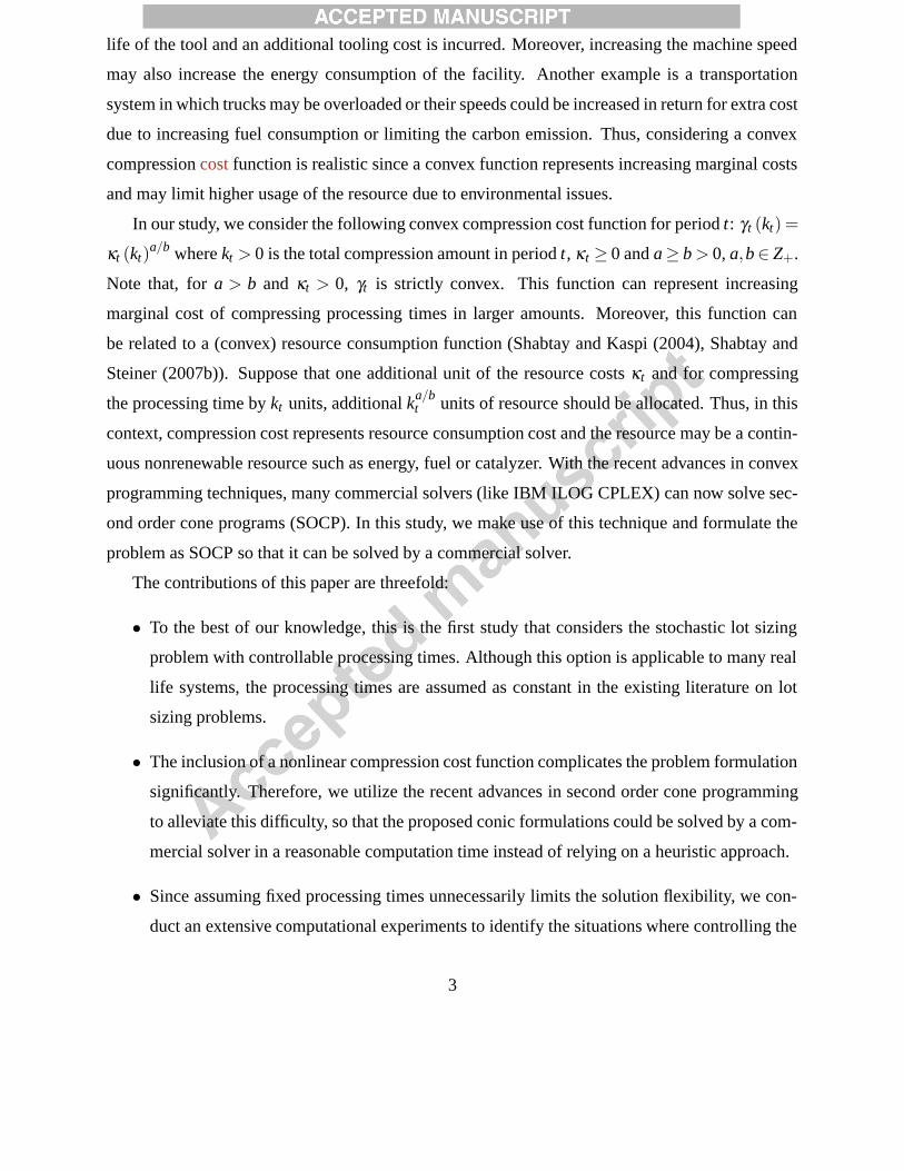
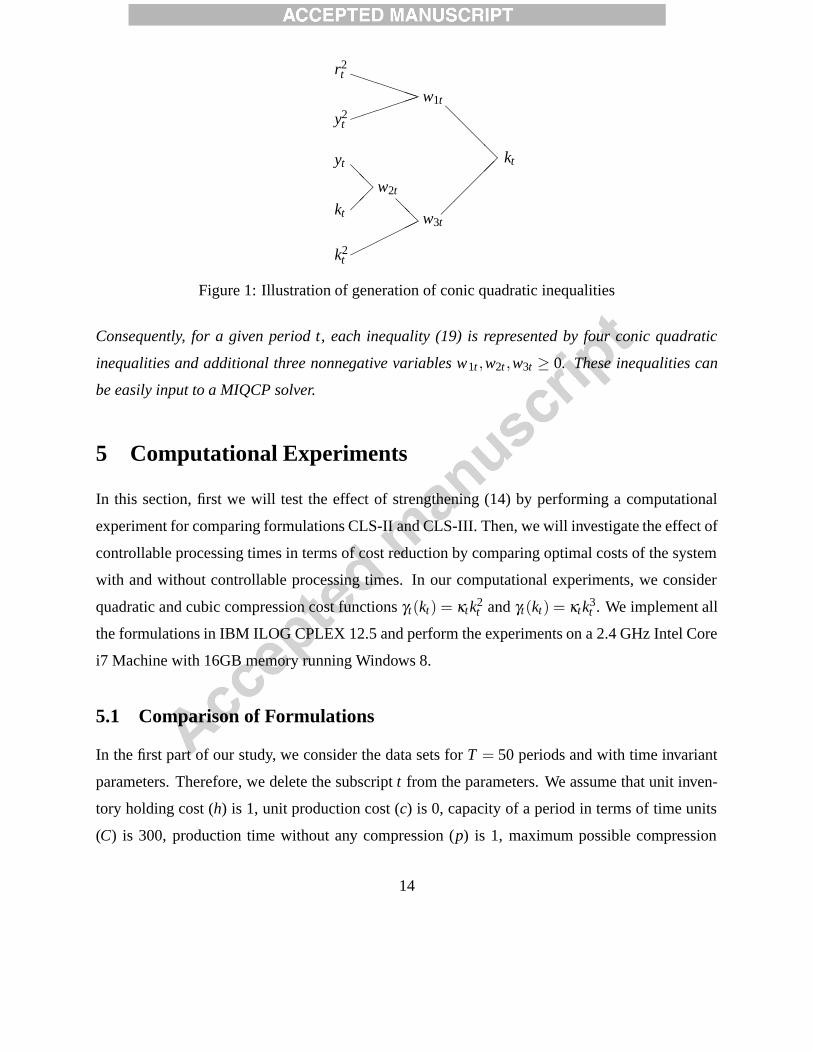
Figure 1 illustrates the generation of these inequalities.

These constraints can be represented by the following conic quadratic inequalities:

4w21t +(rt − yt)

2 ≤ (rt + yt)2 ,

4w22t +(yt − kt)

2 ≤ (yt + kt)2 ,

4w23t +(w2t − kt)

2 ≤ (w2t + kt)2 ,

4k2t +(w1t −w3t)

2 ≤ (w1t +w3t)2 .

13

k2t

kt

yt

y2t

r2t ������

������ w1t

��

��

w2t

��

������ w3t

����

�����

kt

Figure 1: Illustration of generation of conic quadratic inequalities

Consequently, for a given period t, each inequality (19) is represented by four conic quadratic

inequalities and additional three nonnegative variables w1t ,w2t ,w3t ≥ 0. These inequalities can

be easily input to a MIQCP solver.

5 Computational Experiments

In this section, first we will test the effect of strengthening (14) by performing a computational

experiment for comparing formulations CLS-II and CLS-III. Then, we will investigate the effect of

controllable processing times in terms of cost reduction by comparing optimal costs of the system

with and without controllable processing times. In our computational experiments, we consider

quadratic and cubic compression cost functions γt(kt) = κtk2t and γt(kt) = κtk3

t . We implement all

the formulations in IBM ILOG CPLEX 12.5 and perform the experiments on a 2.4 GHz Intel Core

i7 Machine with 16GB memory running Windows 8.

5.1 Comparison of Formulations

In the first part of our study, we consider the data sets for T = 50 periods and with time invariant

parameters. Therefore, we delete the subscript t from the parameters. We assume that unit inven-

tory holding cost (h) is 1, unit production cost (c) is 0, capacity of a period in terms of time units

(C) is 300, production time without any compression (p) is 1, maximum possible compression

14

amount (u) for a unit is 30% of the processing time and coefficient of variation (hereafter CV ) is

10%. We determine the rest of the parameters according to the following values: α ∈ {0.95,0.98},qh∈ {1750,3500,7000},

κh∈ {0.10,0.30},

Cµ p

∈ {3,5} and µt ∼U [0.9µ,1.1µ] for t = 1, . . . ,T .

We set time limit as 2000 seconds.

Most of the commercial solvers, such as IBM ILOG CPLEX, can solve MIP formulations

with a quadratic objective function. Therefore, we also use formulation LS-Q where we keep

the quadratic compression cost function in the objective. We note that LS-Q is the same as LS-

II except that κt rt is replaced by κtk2t in the objective function, constraints (14) and variables

rt , for t = 1, . . . ,T , are removed. We solve LS-Q by CPLEX MIQP. Note that for the quadratic

compression cost function, conic reformulations CLS-II and CLS-III are equivalent to LS-II and

LS-III, respectively. Thus, performance differences of LS-Q and CLS-II will show the effect of

having quadratic terms in the objective function and in the constraints. The effect of proposed

conic strengthening can be observed by comparing CLS-II and CLS-III.

Results of this experiment are given in Tables 1 and 4. In these tables, the percentage gap

between the continuous relaxation at the root node and the optimal solution (rgap) (root gap, here-

after) and the number of branch-and-bound nodes explored are reported. If the solver is terminated

due to the time limit, final gap is given under the column (gap), otherwise solution time is reported

(cpu).

Results of this experiment for quadratic compression cost function are given in Table 1. This

table clearly indicates that CLS-III outperforms CLS-II both in terms of root gap and solution

time. Note that the root gap of CLS-II is twice as large as of the one of CLS-III for some instances.

Moreover, all the instances are solved to optimality in less than 800 seconds by CLS-III (average

solution time is about 200 seconds) whereas CLS-II stops with positive gap due to time limit for 10

out of 24 instances. When we examine the results of LS-Q, an interesting result is obtained: it can

solve an instance within 2 seconds, whereas for another one it stops with 1% optimality gap due

to time limit. Moreover, LS-Q solves 10 instances in less time than CLS-III, but its solution time

seems not so stable. It solves an instance which is solved by CLS-III in about 300 seconds in only

4 seconds. On the other hand, another instance that is solved by CLS-III in less than 40 seconds is

solved by LS-Q in about 2000 seconds. When we investigate the instances in detail, we observe that

when setup cost increases and capacities become tighter, solution time of LS-Q increases. These

15

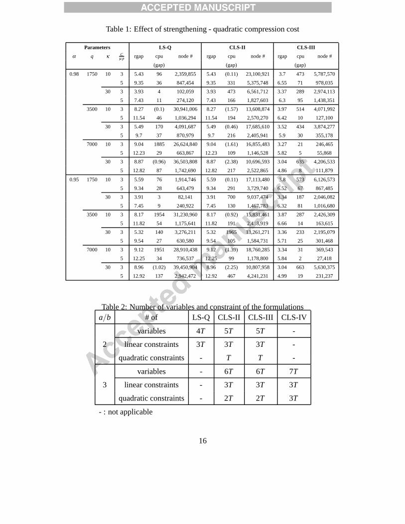
Table 1: Effect of strengthening - quadratic compression cost

Parameters LS-Q CLS-II CLS-III

α q κ Cµ p rgap cpu node # rgap cpu node # rgap cpu node #

(gap) (gap) (gap)

0.98 1750 10 3 5.43 96 2,359,855 5.43 (0.11) 23,100,921 3.7 473 5,787,570

5 9.35 36 847,454 9.35 331 5,375,748 6.55 71 978,035

30 3 3.93 4 102,059 3.93 473 6,561,712 3.37 289 2,974,113

5 7.43 11 274,120 7.43 166 1,827,603 6.3 95 1,438,351

3500 10 3 8.27 (0.1) 30,941,006 8.27 (1.57) 13,608,874 3.97 514 4,071,992

5 11.54 46 1,036,294 11.54 194 2,570,270 6.42 10 127,100

30 3 5.49 170 4,091,687 5.49 (0.46) 17,685,610 3.52 434 3,874,277

5 9.7 37 870,979 9.7 216 2,405,941 5.9 30 355,178

7000 10 3 9.04 1885 26,624,840 9.04 (1.61) 16,855,483 3.27 21 246,465

5 12.23 29 663,867 12.23 109 1,146,528 5.82 5 55,868

30 3 8.87 (0.96) 36,503,808 8.87 (2.38) 10,696,593 3.04 635 4,206,533

5 12.82 87 1,742,690 12.82 217 2,522,865 4.86 8 111,879

0.95 1750 10 3 5.59 76 1,914,746 5.59 (0.11) 17,113,480 3.8 573 6,126,573

5 9.34 28 643,479 9.34 291 3,729,740 6.52 67 867,485

30 3 3.91 3 82,141 3.91 700 9,037,474 3.34 187 2,046,082

5 7.45 9 240,922 7.45 130 1,467,783 6.32 81 1,016,680

3500 10 3 8.17 1954 31,230,960 8.17 (0.92) 15,831,461 3.87 287 2,426,309

5 11.82 54 1,175,641 11.82 191 2,418,919 6.66 14 163,615

30 3 5.32 140 3,276,211 5.32 1965 13,261,271 3.36 233 2,195,079

5 9.54 27 630,580 9.54 105 1,584,731 5.71 25 301,468

7000 10 3 9.12 1951 28,910,438 9.12 (1.39) 18,760,285 3.34 31 369,543

5 12.25 34 736,537 12.25 99 1,178,800 5.84 2 27,418

30 3 8.96 (1.02) 39,450,904 8.96 (2.25) 10,807,958 3.04 663 5,630,375

5 12.92 137 2,942,472 12.92 467 4,241,231 4.99 19 231,237

Table 2: Number of variables and constraint of the formulationsa/b # of LS-Q CLS-II CLS-III CLS-IV

variables 4T 5T 5T -

2 linear constraints 3T 3T 3T -

quadratic constraints - T T -

variables - 6T 6T 7T

3 linear constraints - 3T 3T 3T

quadratic constraints - 2T 2T 3T

- : not applicable

16

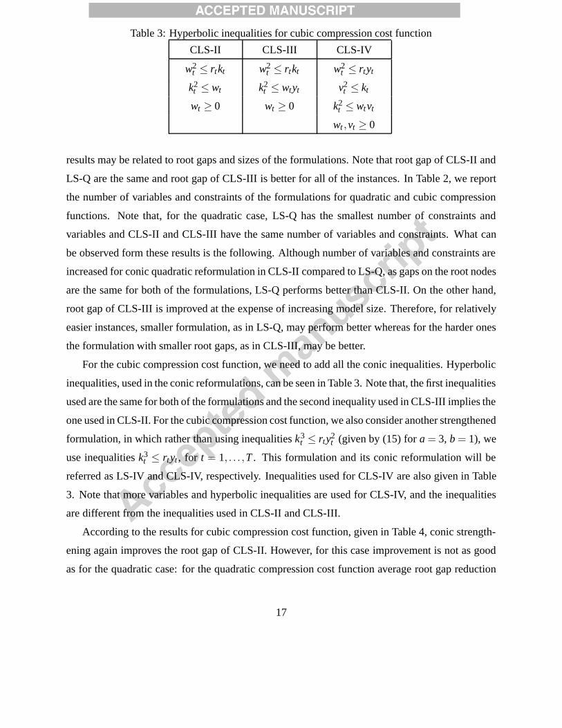
Table 3: Hyperbolic inequalities for cubic compression cost function

CLS-II CLS-III CLS-IV

w2t ≤ rtkt w2

t ≤ rtkt w2t ≤ rtyt

k2t ≤ wt k2

t ≤ wtyt v2t ≤ kt

wt ≥ 0 wt ≥ 0 k2t ≤ wtvt

wt ,vt ≥ 0

results may be related to root gaps and sizes of the formulations. Note that root gap of CLS-II and

LS-Q are the same and root gap of CLS-III is better for all of the instances. In Table 2, we report

the number of variables and constraints of the formulations for quadratic and cubic compression

functions. Note that, for the quadratic case, LS-Q has the smallest number of constraints and

variables and CLS-II and CLS-III have the same number of variables and constraints. What can

be observed form these results is the following. Although number of variables and constraints are

increased for conic quadratic reformulation in CLS-II compared to LS-Q, as gaps on the root nodes

are the same for both of the formulations, LS-Q performs better than CLS-II. On the other hand,

root gap of CLS-III is improved at the expense of increasing model size. Therefore, for relatively

easier instances, smaller formulation, as in LS-Q, may perform better whereas for the harder ones

the formulation with smaller root gaps, as in CLS-III, may be better.

For the cubic compression cost function, we need to add all the conic inequalities. Hyperbolic

inequalities, used in the conic reformulations, can be seen in Table 3. Note that, the first inequalities

used are the same for both of the formulations and the second inequality used in CLS-III implies the

one used in CLS-II. For the cubic compression cost function, we also consider another strengthened

formulation, in which rather than using inequalities k3t ≤ rty2

t (given by (15) for a = 3, b = 1), we

use inequalities k3t ≤ rtyt , for t = 1, . . . ,T . This formulation and its conic reformulation will be

referred as LS-IV and CLS-IV, respectively. Inequalities used for CLS-IV are also given in Table

3. Note that more variables and hyperbolic inequalities are used for CLS-IV, and the inequalities

are different from the inequalities used in CLS-II and CLS-III.

According to the results for cubic compression cost function, given in Table 4, conic strength-

ening again improves the root gap of CLS-II. However, for this case improvement is not as good

as for the quadratic case: for the quadratic compression cost function average root gap reduction

17

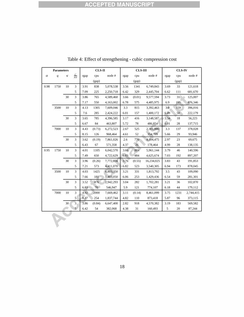
Table 4: Effect of strengthening - cubic compression cost

Parameters CLS-II CLS-III CLS-IV

α q κ Cµ p rgap cpu node # rgap cpu node # rgap cpu node #

(gap) (gap) (gap)

0.98 1750 10 3 3.91 838 5,078,538 3.56 1341 6,749,843 3.69 33 121,618

5 7.09 225 2,250,718 6.42 329 2,445,704 6.62 111 681,670

30 3 3.86 765 4,589,460 3.66 (0.01) 9,577,594 3.73 31 125,007

5 7.17 550 4,163,002 6.78 575 4,485,975 6.9 195 876,346

3500 10 3 4.13 1305 7,609,046 3.3 815 3,392,463 3.6 159 396,016

5 7.6 285 2,424,222 6.01 157 1,400,172 6.49 50 222,179

30 3 3.65 785 4,396,585 3.17 416 3,148,587 3.34 18 56,223

5 6.67 84 463,807 5.72 78 486,854 6.01 28 137,715

7000 10 3 4.43 (0.73) 6,272,523 2.67 525 2,301,886 3.3 137 378,028

5 8.15 126 968,464 4.61 52 354,709 5.66 29 93,946

30 3 3.62 (0.19) 7,861,026 2.6 770 4,104,475 2.97 23 69,675

5 6.43 67 571,358 4.37 26 178,464 4.99 28 138,135

0.95 1750 10 3 4.01 1105 6,042,570 3.66 884 5,961,144 3.79 46 140,596

5 7.49 650 4,722,629 6.83 484 4,625,674 7.03 192 897,207

30 3 3.96 (0.26) 7,772,856 3.76 (0.55) 16,234,025 3.83 43 191,853

5 7.21 573 4,411,070 6.82 523 3,540,305 6.94 173 878,045

3500 10 3 4.03 1425 6,803,350 3.21 331 1,813,792 3.5 43 109,090

5 7.66 181 1,403,050 6.06 253 1,429,436 6.54 59 281,301

30 3 3.52 476 2,942,293 3.04 282 1,702,281 3.21 36 102,870

5 6.83 70 546,947 5.9 121 774,107 6.18 44 179,112

7000 10 3 4.92 2000 7,669,462 3.11 (0.14) 8,461,099 3.75 1231 2,744,415

5 8.37 254 1,837,744 4.82 110 873,418 5.87 96 373,115

30 3 3.86 (0.84) 6,647,400 2.82 918 4,570,382 3.19 183 569,582

5 6.42 54 382,068 4.38 31 160,493 5 20 87,244

18

is about 4% (40%, relatively), but for the cubic compression cost function it is about 1% (20%,

relatively). Although root gap for CLS-III is the best, the performance of CLS-IV could be viewed

as better since it solves all the instances within the time limit and its average solution time is about

120 seconds. The difference between CLS-II and CLS-III is not clear for this case: 18 out of 24

instances are solved by both of the formulations, and 13 of them are solved in less time by CLS-III.

There is one instance that is solved by CLS-II but not by CLS-III, but three of the instances that

cannot be solved by CLS-II are solved by CLS-III. Moreover, if we investigate the results in more

detail, we can observe that CLS-III mostly performs better than CLS-II in harder instances (with

large setup costs and tighter capacities). The number of variables and constraints for these formu-

lations are also given in Table 2. Note that, the number of variables and constraints of CLS-IV are

larger than the ones for CLS-II and CLS-III, and the latter two formulations have equal number of

variables and constraints. Although the size of CLS-IV is larger, the root gap of this formulation

is not the best. On the other hand, this formulation performs better in terms of solution times.

This situation may be caused by the different types of conic inequalities added to this formulation

(Table 2).

Overall, we observed that conic strengthening improves root gaps. This improvement is more

definite for the quadratic compression cost function, since CLS-III outperforms CLS-II for this

case. But for the cubic compression cost function, CLS-IV, in which more conic inequalities are

used, outperforms CLS-III, for our instances. In summary, by utilizing second order cone pro-

gramming, we could solve the relatively practical sizes of stochastic capacitated lot sizing problem

with a nonlinear compression cost function in a reasonable computation time instead of relying on

a heuristic approach.

5.2 Effect of Controllable Processing Times

Controlling the capacity of the system can be a beneficial tool to hedge against demand uncertainty.

For this purpose, in this section, we report the results of several experiments to show the benefits of

controlling processing times under different uncertainty/cost/capacity settings. In order to achieve

this, we will compare the optimal costs for the problem with and without controllable processing

times, which will be called as LS-C and LS, respectively, and report the cost reduction. In this

part, we again assume that all the parameters are time invariant, and the compression cost function

19

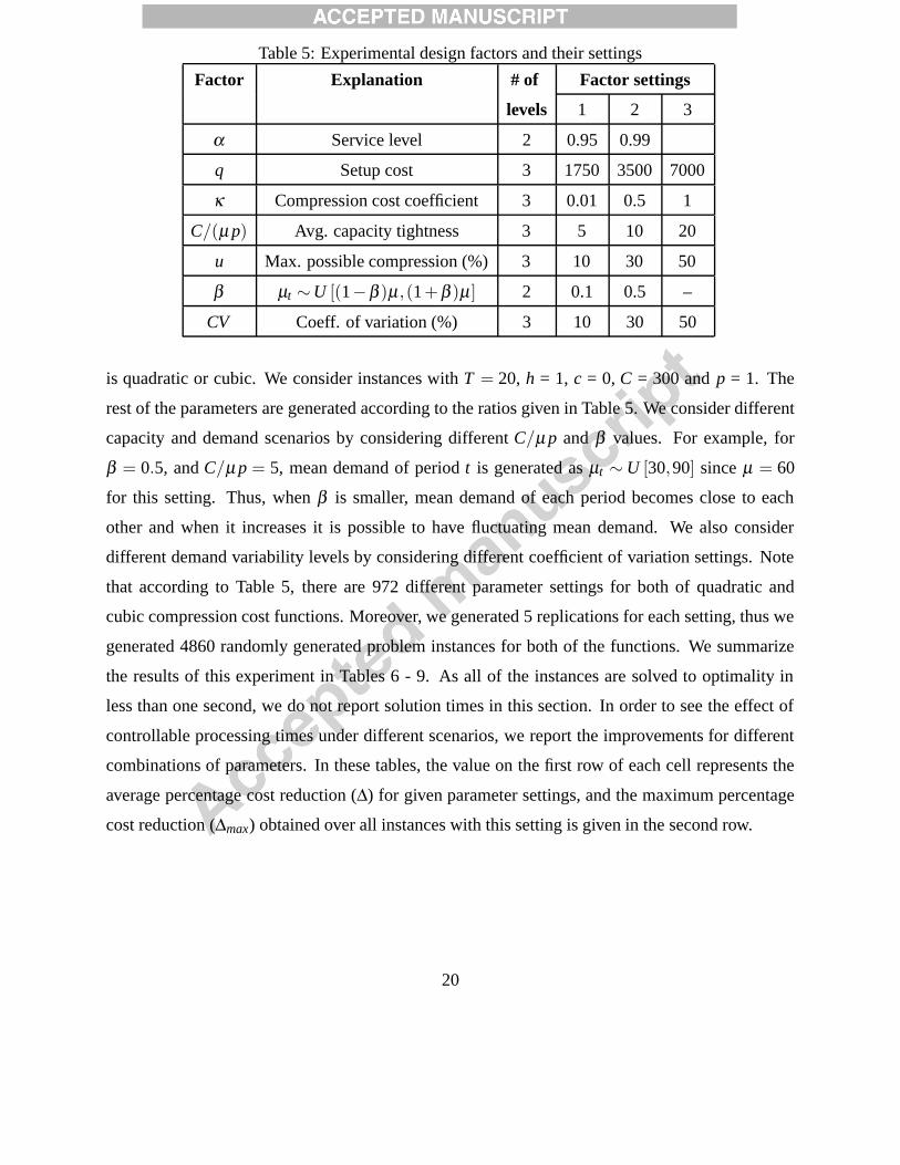
Table 5: Experimental design factors and their settings

Factor Explanation # of Factor settings

levels 1 2 3

α Service level 2 0.95 0.99

q Setup cost 3 1750 3500 7000

κ Compression cost coefficient 3 0.01 0.5 1

C/(µ p) Avg. capacity tightness 3 5 10 20

u Max. possible compression (%) 3 10 30 50

β µt ∼U [(1−β )µ,(1+β )µ] 2 0.1 0.5 –

CV Coeff. of variation (%) 3 10 30 50

is quadratic or cubic. We consider instances with T = 20, h = 1, c = 0, C = 300 and p = 1. The

rest of the parameters are generated according to the ratios given in Table 5. We consider different

capacity and demand scenarios by considering different C/µ p and β values. For example, for

β = 0.5, and C/µ p = 5, mean demand of period t is generated as µt ∼ U [30,90] since µ = 60

for this setting. Thus, when β is smaller, mean demand of each period becomes close to each

other and when it increases it is possible to have fluctuating mean demand. We also consider

different demand variability levels by considering different coefficient of variation settings. Note

that according to Table 5, there are 972 different parameter settings for both of quadratic and

cubic compression cost functions. Moreover, we generated 5 replications for each setting, thus we

generated 4860 randomly generated problem instances for both of the functions. We summarize

the results of this experiment in Tables 6 - 9. As all of the instances are solved to optimality in

less than one second, we do not report solution times in this section. In order to see the effect of

controllable processing times under different scenarios, we report the improvements for different

combinations of parameters. In these tables, the value on the first row of each cell represents the

average percentage cost reduction (∆) for given parameter settings, and the maximum percentage

cost reduction (∆max) obtained over all instances with this setting is given in the second row.

20

5.2.1 Effect of Setup Costs

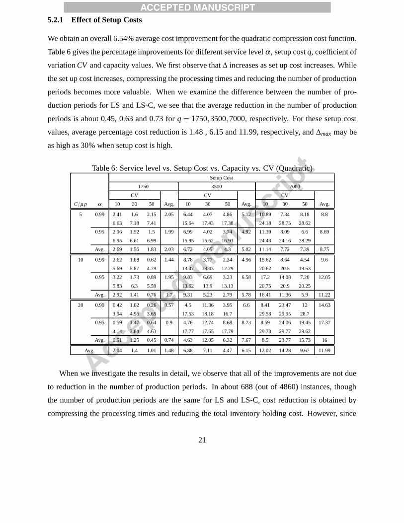
We obtain an overall 6.54% average cost improvement for the quadratic compression cost function.

Table 6 gives the percentage improvements for different service level α , setup cost q, coefficient of

variation CV and capacity values. We first observe that ∆ increases as set up cost increases. While

the set up cost increases, compressing the processing times and reducing the number of production

periods becomes more valuable. When we examine the difference between the number of pro-

duction periods for LS and LS-C, we see that the average reduction in the number of production

periods is about 0.45, 0.63 and 0.73 for q = 1750,3500,7000, respectively. For these setup cost

values, average percentage cost reduction is 1.48 , 6.15 and 11.99, respectively, and ∆max may be

as high as 30% when setup cost is high.

Table 6: Service level vs. Setup Cost vs. Capacity vs. CV (Quadratic)Setup Cost

1750 3500 7000

CV CV CV

C/µ p α 10 30 50 Avg. 10 30 50 Avg. 10 30 50 Avg.

5 0.99 2.41 1.6 2.15 2.05 6.44 4.07 4.86 5.12 10.89 7.34 8.18 8.8

6.63 7.18 7.41 15.64 17.43 17.38 24.18 28.75 28.62

0.95 2.96 1.52 1.5 1.99 6.99 4.02 3.74 4.92 11.39 8.09 6.6 8.69

6.95 6.61 6.99 15.95 15.62 16.91 24.43 24.16 28.29

Avg. 2.69 1.56 1.83 2.03 6.72 4.05 4.3 5.02 11.14 7.72 7.39 8.75

10 0.99 2.62 1.08 0.62 1.44 8.78 3.77 2.34 4.96 15.62 8.64 4.54 9.6

5.69 5.87 4.79 13.47 13.43 12.29 20.62 20.5 19.53

0.95 3.22 1.73 0.89 1.95 9.83 6.69 3.23 6.58 17.2 14.08 7.26 12.85

5.83 6.3 5.59 13.62 13.9 13.13 20.75 20.9 20.25

Avg. 2.92 1.41 0.76 1.7 9.31 5.23 2.79 5.78 16.41 11.36 5.9 11.22

20 0.99 0.42 1.02 0.26 0.57 4.5 11.36 3.95 6.6 8.41 23.47 12 14.63

3.94 4.96 3.65 17.53 18.18 16.7 29.58 29.95 28.7

0.95 0.59 1.47 0.64 0.9 4.76 12.74 8.68 8.73 8.59 24.06 19.45 17.37

4.14 3.84 4.63 17.77 17.65 17.79 29.78 29.77 29.62

Avg. 0.51 1.25 0.45 0.74 4.63 12.05 6.32 7.67 8.5 23.77 15.73 16

Avg. 2.04 1.4 1.01 1.48 6.88 7.11 4.47 6.15 12.02 14.28 9.67 11.99

When we investigate the results in detail, we observe that all of the improvements are not due

to reduction in the number of production periods. In about 688 (out of 4860) instances, though

the number of production periods are the same for LS and LS-C, cost reduction is obtained by

compressing the processing times and reducing the total inventory holding cost. However, since

21

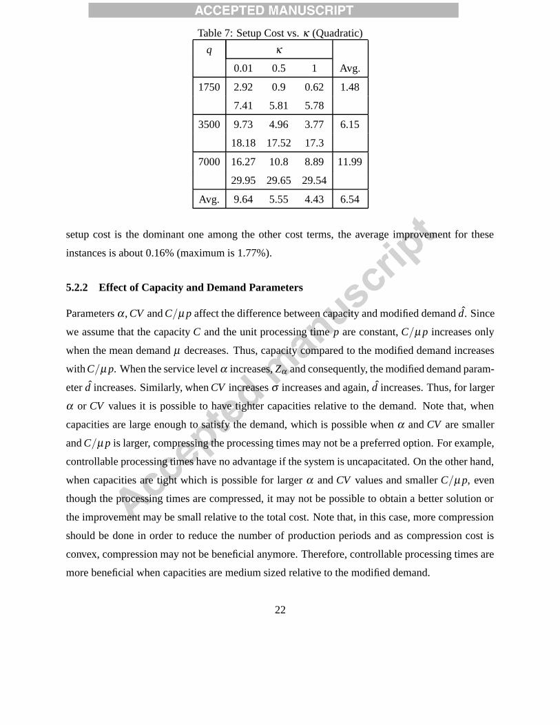
Table 7: Setup Cost vs. κ (Quadratic)

q κ

0.01 0.5 1 Avg.

1750 2.92 0.9 0.62 1.48

7.41 5.81 5.78

3500 9.73 4.96 3.77 6.15

18.18 17.52 17.3

7000 16.27 10.8 8.89 11.99

29.95 29.65 29.54

Avg. 9.64 5.55 4.43 6.54

setup cost is the dominant one among the other cost terms, the average improvement for these

instances is about 0.16% (maximum is 1.77%).

5.2.2 Effect of Capacity and Demand Parameters

Parameters α , CV and C/µ p affect the difference between capacity and modified demand d. Since

we assume that the capacity C and the unit processing time p are constant, C/µ p increases only

when the mean demand µ decreases. Thus, capacity compared to the modified demand increases

with C/µ p. When the service level α increases, Zα and consequently, the modified demand param-

eter d increases. Similarly, when CV increases σ increases and again, d increases. Thus, for larger

α or CV values it is possible to have tighter capacities relative to the demand. Note that, when

capacities are large enough to satisfy the demand, which is possible when α and CV are smaller

and C/µ p is larger, compressing the processing times may not be a preferred option. For example,

controllable processing times have no advantage if the system is uncapacitated. On the other hand,

when capacities are tight which is possible for larger α and CV values and smaller C/µ p, even

though the processing times are compressed, it may not be possible to obtain a better solution or

the improvement may be small relative to the total cost. Note that, in this case, more compression

should be done in order to reduce the number of production periods and as compression cost is

convex, compression may not be beneficial anymore. Therefore, controllable processing times are

more beneficial when capacities are medium sized relative to the modified demand.

22

Results given in Table 6 confirm the observations explained above. For example, for C/µ p = 5

or 10, ∆ is maximum when CV = 10 and if C/µ p is increased to 20, ∆ is larger for CV = 30.

α and the coefficient of variation have the same effect on the modified demand, but according

to Table 6, ∆ is more affected by the changes in the coefficient of variation. Note that, the changes

in CV affect the modified demand in larger amounts and this is the reason of larger changes of ∆

with respect to CV .

Table 8: Capacity vs. mean demand variability vs. max. possible compression (Quadratic)

β

10 50Cµ p u u

10 30 50 Avg. 10 30 50 Avg.

5 3.66 6.08 7.18 5.64 3.08 5.15 6.43 4.89

12.98 24.43 28.62 13.1 23.75 28.75

10 5.47 8.07 8.07 7.2 3.35 6.16 6.26 5.26

20.75 20.75 20.75 20.9 20.9 20.9

20 6.39 8.7 8.7 7.93 5.91 9.54 9.54 8.33

29.77 29.77 29.77 29.95 29.95 29.95

Avg. 5.17 7.62 7.98 6.92 4.11 6.95 7.41 6.16

When we investigate the results in more detail, we observe that as the capacity increases, the

total cost of LS decreases, in general. Therefore, even though the cost reduction due to controllable

processing times is the same for different capacity settings, as ∆ indicates the percentage cost

improvement, ∆ may be higher for larger capacity settings. An example of this situation is observed

for CV = 10 and C/µ p = 5 or 10.

To sum up, according to Table 6, we can conclude that controllable processing times are more

beneficial when setup costs are high and the difference between the capacities and the modified

demand is medium sized.

23

5.2.3 Other Parameters

Table 7 shows the percentage improvements for setup cost and compression cost coefficient κ .

When κ increases, as it is expected, the compression cost increases and consequently, the cost

reduction that can be obtained by compressing the processing times decreases. But note that when

setup cost increases, it is more beneficial to compress the processing times, even with larger κ , and

it is possible to have a reduction of 29%.

In Table 8, the percentage improvements for different capacity levels, maximum possible com-

pression amounts (u) and mean demand scenarios are given. As expected, if u increases, the cost

difference between LS and LS-C, and consequently, ∆ may increase. If capacities are large enough,

larger u values may not change the optimal production plan. Note that, ∆ and ∆max are the same

for different u values when capacities are large enough. Moreover, average cost and number of

production periods differences are the same for these settings. On the other hand, when capacity is

tighter, increasing the maximum possible compression amount increases the improvement.

According to Table 8, effect of β on ∆ is relatively small. More improvement is observed

when capacities are looser and mean demand fluctuates more or capacities are tighter and mean

demand is stable. When we examine the results in detail, we obtain that when capacity is large

enough and mean demand is stable, without reducing processing times an optimal production plan

can be observed. Moreover, we note that in none of the test instances with C/µ p = 20, CV = 10

and β = 0.1, a cost reduction is observed. But this setting is an extreme case as capacity is large

enough and with only one production period all the necessary demand is produced.

5.2.4 Cubic Compression Cost Function

In Table 9, results for the cubic compression cost function are given. In this table, we report the

percentage improvements for different service level α , setup cost q, coefficient of variation CV

and capacity values. The average improvement is 3.03%. When the compression cost function is

changed from quadratic to cubic, ∆ decreases since compression becomes more expensive (when

kt ≥ 1). Although the average improvement decreases, behavior of ∆ is very similar to one of

the quadratic case. Note that, for some settings ∆max may be as high as the one for quadratic

compression cost function, but also for some parameter combinations it may be zero. As similar

results are obtained for this case, we do not report the impact of other problem parameters in detail.

24

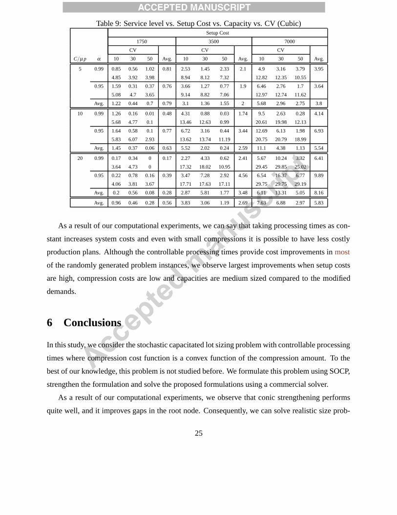
Table 9: Service level vs. Setup Cost vs. Capacity vs. CV (Cubic)Setup Cost

1750 3500 7000

CV CV CV

C/µ p α 10 30 50 Avg. 10 30 50 Avg. 10 30 50 Avg.

5 0.99 0.85 0.56 1.02 0.81 2.53 1.45 2.33 2.1 4.9 3.16 3.79 3.95

4.85 3.92 3.98 8.94 8.12 7.32 12.82 12.35 10.55

0.95 1.59 0.31 0.37 0.76 3.66 1.27 0.77 1.9 6.46 2.76 1.7 3.64

5.08 4.7 3.65 9.14 8.82 7.06 12.97 12.74 11.62

Avg. 1.22 0.44 0.7 0.79 3.1 1.36 1.55 2 5.68 2.96 2.75 3.8

10 0.99 1.26 0.16 0.01 0.48 4.31 0.88 0.03 1.74 9.5 2.63 0.28 4.14

5.68 4.77 0.1 13.46 12.63 0.99 20.61 19.98 12.13

0.95 1.64 0.58 0.1 0.77 6.72 3.16 0.44 3.44 12.69 6.13 1.98 6.93

5.83 6.07 2.93 13.62 13.74 11.19 20.75 20.79 18.99

Avg. 1.45 0.37 0.06 0.63 5.52 2.02 0.24 2.59 11.1 4.38 1.13 5.54

20 0.99 0.17 0.34 0 0.17 2.27 4.33 0.62 2.41 5.67 10.24 3.32 6.41

3.64 4.73 0 17.32 18.02 10.95 29.45 29.85 25.02

0.95 0.22 0.78 0.16 0.39 3.47 7.28 2.92 4.56 6.54 16.37 6.77 9.89

4.06 3.81 3.67 17.71 17.63 17.11 29.75 29.75 29.19

Avg. 0.2 0.56 0.08 0.28 2.87 5.81 1.77 3.48 6.11 13.31 5.05 8.16

Avg. 0.96 0.46 0.28 0.56 3.83 3.06 1.19 2.69 7.63 6.88 2.97 5.83

As a result of our computational experiments, we can say that taking processing times as con-

stant increases system costs and even with small compressions it is possible to have less costly

production plans. Although the controllable processing times provide cost improvements in most

of the randomly generated problem instances, we observe largest improvements when setup costs

are high, compression costs are low and capacities are medium sized compared to the modified

demands.

6 Conclusions

In this study, we consider the stochastic capacitated lot sizing problem with controllable processing

times where compression cost function is a convex function of the compression amount. To the

best of our knowledge, this problem is not studied before. We formulate this problem using SOCP,

strengthen the formulation and solve the proposed formulations using a commercial solver.

As a result of our computational experiments, we observe that conic strengthening performs

quite well, and it improves gaps in the root node. Consequently, we can solve realistic size prob-

25

lems in a reasonable computation time using an exact approach. Moreover, these formulations

maybe further improved by adding new valid inequalities in a future research.

Although controllable processing times may be applicable to many real life production and

inventory systems, processing times are assumed as constant in the classical lot sizing problems.

In the second part of our computational experiments, we show that this assumption causes higher

system costs. We observe that controllable processing times are more valuable when the system

has medium sized capacities and larger setup costs. By relaxing the fixed processing time assump-

tion and by utilizing the recent advances in second order cone programming, we could decrease the

overall production costs significantly. Although we explore these results for the static uncertainty

strategy under α service level constraints, these results are also applicable to the deterministic lot

sizing problem. As a future research direction, it is possible to consider the same problem under

different settings like considering different uncertainty strategies, joint chance constraints or using

multistage stochastic programming approach to deal with different scenarios.

Acknowledgments The authors thank the area editor, the associate editor, and anonymous refer-

ees for their constructive comments and suggestions that significantly improved this paper. This

research is supported by TUBITAK Project no 112M220. The research of the second author is

supported by the Turkish Academy of Sciences.

References

S. Ahmed, A.J. King, and G. Parija. A multi-stage stochastic integer programming approach for

capacity expansion under uncertainty. Journal of Global Optimization, 26:3 – 24, 2003.

M.S. Akturk, A. Atamturk, and S. Gurel. A strong conic quadratic reformulation for machine-job

assignment with controllable processing times. Operations Research Letters, 37(3):187–191,

2009.

A. Atamturk and D.S. Hochbaum. Capacity acquisition, subcontracting, and lot sizing. Manage-

ment Science, 47(8):1081–1100, 2001.

26

A. Ben-Tal and A. Nemirovski. Lectures on modern convex optimization: analysis, algorithms,

and engineering applications. Society for Industrial and Applied Mathematics, 2001.

J.H. Bookbinder and J-Y. Tan. Strategies for probabilistic lot-sizing problem with service-level

constraints. Management Science, 34(9):1096 – 1108, 1988.

F.Y. Chen and D. Krass. Inventory models with minimal service level constraints. European

Journal of Operational Research, 134(1):120–140, 2001.

K.L Croxton, B. Gendron, and T.L. Magnanti. A comparison of mixed-integer programming mod-

els for nonconvex piecewise linear cost minimization problems. Management Science, 49(9):

1268–1273, 2003.

M. Florian, J.K. Lenstra, and A.H.G. Rinnooy Kan. Deterministic production planning: Algo-

rithms and complexity. Management Science, 26(7):669–679, 1980.

S. Gurel, E. Korpeoglu, and M.S. Akturk. An anticipative scheduling approach with controllable

processing times. Computers & Operations Research, 37(6):1002–1013, 2010.

S. Helber, F. Sahling, and K. Schimmelpfeng. Dynamic capacitated lot sizing with random demand

and dynamic safety stocks. OR Spectrum, 35:75 – 105, 2013.

K. Jansen and M. Mastrolilli. Approximation schemes for parallel machine scheduling problems

with controllable processing times. Computers & Operations Research, 31(10):1565–1581,

2004.

A. Jeang. Simultaneous determination of production lot size and process parameters under process

deterioration and process breakdown. Omega, 40:774–781, 2012.

B. Karimi, S.M.T. Fatemi Ghomi, and J.M. Wilson. The capacitated lot sizing problem: a review

of models and algorithms. Omega, 31(5):365–378, 2003.

R.K. Kayan and M.S. Akturk. A new bounding mechanism for the CNC machine scheduling

problems with controllable processing times. European Journal of Operational Research, 167

(3):624–643, 2005.

27

E. Koca, H. Yaman, and M.S. Akturk. Lot sizing with piecewise concave production costs. IN-

FORMS Journal on Computing, 26(4):767–779, 2014.

J.B. Laserre, C. Bes, and F. Roubellat. The stochastic discrete dynamic lot size problem: an open-

loop solution. Operations Research, 33(3):684 – 689, 1985.

H. Luss. Operations research and capacity expansion problems: A survey. Operations Research,

30(5):907–947, 1982.

Y. Merzifonluoglu, J. Geunes, and H. Romeijn. Integrated capacity, demand, and production plan-

ning with subcontracting and overtime options. Naval Research Logistics, 54(4):433–447, 2007.

S. Nahmias. Production and Operations Analysis. McGraw-Hill/Irwin, 1993.

U. Ozen, M.K. Dogru, and S.A. Tarım. Static-dynamic uncertainty strategy for a single-item

stochastic inventory control problem. Omega, 40:348 – 357, 2012.

Y. Pochet and L.A. Wolsey. Production Planning by Mixed Integer Programming. Springer, 2006.

S. Rajagopalan and J.M. Swaminathan. A coordinated production planning model with capacity

expansion and inventory management. Management Science, 47(11):1562–1580, 2001.

P. Robinson, A. Narayanan, and F. Sahin. Coordinated deterministic dynamic demand lot-sizing

problem: A review of models and algorithms. Omega, 37(1):3–15, 2009.

R. Rossi, O.A. Kılıc, and S.A. Tarım. Piecewise linear approximations for the static-dynamic

uncertainty strategy in stochastic lot-sizing. to appear in Omega, 2014.

D. Shabtay and M. Kaspi. Minimizing the total weighted flow time in a single machine with

controllable processing times. Computers & Operations Research, 31(13):2279–2289, 2004.

D. Shabtay and M. Kaspi. Parallel machine scheduling with a convex resource consumption func-

tion. European Journal of Operational Research, 173(1):92–107, 2006.

D. Shabtay and G. Steiner. A survey of scheduling with controllable processing times. Discrete

Applied Mathematics, 155(13):1643–1666, 2007a.

28

D. Shabtay and G. Steiner. Single machine batch scheduling to minimize total completion time

and resource consumption costs. Journal of Scheduling, 10(4-5):255–261, 2007b.

D.X. Shaw and A.P.M. Wagelmans. An algorithm for single-item capacitated economic lot sizing

with piecewise linear production costs and general holding costs. Management Science, 44(6):

831–838, 1998.

E. Silver. Inventory control under a probabilistic time-varying, demand pattern. AIIE Transactions,

10(4):371–379, 1978.

C. Sox. Dynamic lot sizing problem with demand and non-stationary demand. Operations Re-

search Letters, 20:155 – 164, 1997.

S.A. Tarım and B.G. Kingsman. The stochastic dynamic production/inventory lot-sizing problem

with service-level constraints. International Journal of Production Economics, 88:105 – 119,

2004.

H. Tempelmeier. A column generation heuristic for dynamic capacitated lot sizing with random

demand under a fill rate constraint. Omega, 39:627 – 633, 2011.

H. Tunc, O. Kılıc, S.A. Tarım, and B. Eksioglu. The cost of using stationary inventory policies

when demand is non-stationary. Omega, 39(4):410–415, 2011.

H. Tunc, O.A. Kılıc, S.A. Tarım, and B. Eksioglu. A simple approach for assessing the cost of

system nervousness. International Journal of Production Economics, 141(2):619–625, 2013.

H. Tunc, O.A. Kılıc, S.A. Tarım, and B. Eksioglu. A reformulation for the stochastic lot sizing

problem with service-level constraints. Operations Research Letters, 42(2):161–165, 2014.

A. Turkcan, M.S. Akturk, and R.H. Storer. Predictive/reactive scheduling with controllable pro-

cessing times and earliness-tardiness penalties. IIE Transactions, 41(12):1080–1095, 2009.

V. Vargas. An optimal solution for the stochastic version of the Wagner-Whitin dynamic lot-size

model. European Journal of Operational Research, 198:447 – 451, 2009.

R.G. Vickson. Two single machine sequencing problems involving controllable job processing

times. AIIE transactions, 12(3):258–262, 1980.

29

H.M. Wagner and T.M. Whitin. Dynamic version of the economic lot size model. Management

Science, 5(1):89 – 96, 1958.

C. Yan, Y. Liao, and A. Banerjee. Multi-product lot scheduling with backordering and shelf-life

constraints. Omega, 41:510–516, 2013.

30