INTELLIGENT TRACKING TECHNIQUES

1m

1 •FOURTH QUARTERLY REPORT

for

September 30, 1979

ia

CONTRACT: DAAK 70-78-C-0167

Presented to

Night Vision and Electro-Optics Laboratory"" Fort Belvoir, Virginia 22060

Submitted by .S4. •;

Westinghouse Electric Corporation A"Systems Development DivisionBaltimore, Maryland 21203

.. j

80 8 008

9: , .. 80 7 8 008..i

A4

"L N INTELLIGENT TRACKING TECHNIQUES

[ !':I

FOURTH QUARTERLY REPORT

for

September 30, 1979

CONTRACT: DAAK 70-78-C-0167

SPresented to

-.. Night Vision and Electro-Optics LaboratoryFort Belvoir, Virginia 22060

Submitted by

Westinghouse Electric Corporation-.Systems Development Division

Baltimore, Maryland 21203

t

won- 7

OA. .

111CURITY CLASSIFICATION OF I HIS PACE (Wbhon 0., EIeZer-.0DOCUENTAION AGEREAD INSTRUCTIONSREPORT DOUETTINPG EFORE COMPLETING F0R4f

1. REPORT NUMBER 2. GOVY ACCESSION NO. 3. RECIPIENT"S CATALOG NUSEiR

1 ~4. T .E~g -- -'~~5. TYPE Of REPORT a PERIOD COVEREDInelgntTakn Techniques i/ Fourth Quarterly Report

Y-Report-July 1, 1979 - Sept. 30, 1979.-ERFRMIN ORO. REPORT NUMBER

2. AUTmOR(A) 111 C~ONTRqACT OR GRANT NUMBER(#)

5T.J. Willett, et.al. -... -7-,06J

9. PERFOR14ING ORGANIZATION NAME AND ADDRESS to. PROGRAM PAI E 'r TC1 ?ASKI ~~~Systems Development Division v AESWR UI UUR

Westinghouse Electric CorporationBaltimore, Maryland 21203 ' '-

11- CONTROLLING OFF ICE NAME AND ADDRESS 12. REPORT DATE

U.S AmySept. 30, 1979Night Vision and Electro-Optics Laboratory 13. NUMBER Or PAGESFort Belvoir, Virginia- 22O0 63

14.MONT~ORING AGENCY NAME. 6 AOURCSS(it different from Controlling Ollie*) III. SECURITY CLASS. (at hi rAepotpn)

r1 .DITIUINSTATEMENT (of tis.~a~c Repo t) e nCok2,i lIitIe ~el

'A A,

'I diit Hh epTflOT

19. KEY WORDS (Continue on reverse wd. If necessary and Identity by black number)Automatic Target Cueing TV SensorTarget Recognition Digital Image Processing

ITarget Tracking Correlation TrackingFLIR Sensor Target Homing

0,ABSTIR~r (C!"tInue on W9186 s ide 0: n~eoiaarv and Identity by black nunibe,)

4 ~This is the Fourth (Quarterly Report under a contract to investigatethe design, test, and implementation of a set of algorithms to perform intelli-

1' gent tracking and intelligent target homing on FLIR and TV imagery. Theintelligent tracker will monitor the entire field of view, detect and classifytargets, perform multiple target tracking and predict changes in targetsignature prior to the target's entry into an obscuration. The intelligent.tracking and homing system will also perform target prioritization and1critical aimpoint selection...>dT

DD 1473 EDITION OF I NOV 65 1S OO.OLIETt lA44 o SECURI1TY CLASSIFICATION OF loi;S PAGt 04h-.

~~t5&w ~77'

, iCUMTY CLASSIPICATION Of THIS PA ,E(i7.Whn Date E eo.P..

A system concept was developed for intelligent homing and aimpointselection. The problem was divided into long range homing and aimpointselection and close-in homing and aimpoint selection. Sets of 875-lineFUR imagery were extracted from the NV&EOL data base and exampleswere presented for both categories. The subjects of close-in homing and

* aimpoint selection were further divided into cl6se-in segmentation, close-itarget tracking, and tracking during the transition from long range toclose-in.

4 1

D 't

I

__'A

,.ar

TABLE OF CONTENTS

"[ Page

INTRODUCTION.

1.0 SYSTEM CONCEPT 1-1

1.1 Target Acquisition and Handover 1-31.2 Multiple Target Tracking 1-3

1.3 Target Signature Prediction 1-4

1.4 Reacquisition 1-51.5 Aimpoint Selection 1-5

2.0 WEAPON ANALYSIS 2-1

2.1 Mission Requirements 2-2

2.2 Design Constraints 2-4

2.3 System Design Requirements 2-6

2.4 Body Fixed vs Gimbaled Sensor 2-7

3.0 INTELLIGENT HOMING 3-1i4m

3.1 Related Work 3-1

3.2Extending'Ground Coverage 3-2

3.3 Aimpoint Selection 3-3

3.3.1 exterior based aimpoint selection 3-4

3.3.2 interior based aimpoint selection 3-8

4.0 PRELIMINARY RESULTS 4-1

'0 4.3 Long Range Aimpoint Selection- 4-1

4.2 Close-in Homing and Aimpoint Selection 4-124.2.1 close-in segmentation 4-124.2.2 close-in target tracking 4-204.2.3 tracking during transition 4-34

I.

___________________________________________A -.-! .'- I ' ".'

INTRODUCTION

Under contract to the Army's Night Vision and Electro-Optics Laboratory,

Westinghouse has been investigating the design, test, and implementation of a

set of algorithms to perform intelligent tracking and intelligent target homing

on FLIR and TV imagery. Research has been initiated for the development of an

intelligent target tracking and homing system which will combine target cueing,

target signature prediction, and target tracking techniques for near zero

break lock performance. The intelligent tracker will monitor the entire field

of view, detect and classify targets, perform multiple target tracking, and

predict changes in target signature prior to the target's entry into an obscur-ation. The intelligent tracking and homing system will also perform target

prioritization and critical aimpoint selection. Through the use of VLSI/VHSI

techniques, the intelligent tracker (with inherent target cuer) can be applied

to the fully autonomous munition.

During the fourth quarter, several meetings and a number of phone conver-

sations took place between Westinghouse personnel and Cpt. Reischer of NV&EOL.

A system concept was developed for intelligent homing and aimpoint selection.li • The problem was divided into long range homing and aimpoint selection and

close-in homing and aimpoint selection. Sets of 875 line FLIR imagery were

extracted from the NV&EOL data base and examples were presented for both

categories. The subjects of close-in homing and aimpoint selection were further

divided into c ose-in segmentation, close-in target tracking and tracking during

the transition from long range to close-in. ijWestinghouse personnel participating in this effort include Thomas Willett,

Program Manager, Dr. John Romanski, John Shipley, Leo Kossa, Bill Pleasance,

and Richard Kroupa. Program review and consultation is provided by

Drs. Glenn Tisdale and Azriel Rosenfeld.

1.0 SYSTEM CONCEPT

The purpose of this section is to describe the preliminary intelligent

tracker concept that has evolved during the course of this work. The desired

intelligent tracker functions are:

1. acquisition and track initiation - detect, locate, classify

and prioritize targets automatically and handoff to the internal

tracker (the intellignet tracker concept is assumed to include

both acquisition and tracking);

2. handle multiple targets - track a number of targets in a scene

simultaneously;

3. target signature prediction - predict or anticipate target obscuration

and how the target signature will change as a result of the

obscuration;

4. reacquisition - reacqbire a target at the earliest opportunity following

track break lock, including departure from the field of view;

5. aimpoint selection - determine the critical aimpoint of a target

which may be an interior point within its silhouette.

ii. A video timing diagram is shown in Figure 1-1. Figure 1-2 shows how an

image appears in the frame store device. A block diagram of the system concept

is shown in Figure 1-3.

The heavy vertical lines in Figure 1-1 represent the cued frames and the

lighter vertical lines are the tracked frames. Frame 1 is a cueing frame, and

frames 2, 3, 4, and 5 are tracking frames and then the cycle repeats. Frame 6

is a cueing frame, and frames 7, 8, 9, and 10 are tracking frames. Thus the

complex target cueing function is performed at 0.2 the rate of the simpler tracking

function. Figure 1-2 represents the image in the frarroa store which is divided into jfive horizontal and addressable strips. This is done so that, instead of waiting

for the entire frame to be cued

1-1

t

1 2 3 4 * 6 9 101

CR P:;' " CACA

Figure 1-1. Timing Diagram

I,' I"" 2 '

Figure 1-2. Image In Frame Store RAM

i .i

illFRAUNC

IMAAEIT - FSTORE CL'TORMlllil LL. IIFIINI M. A144vtil Il i L•_ECT.

RATEI S RETCRENCE COMPRELATIOWd

L.. -J TRACKINS LOW

Figure 1-3. System Block Diagram

1-2

before handover to a tracker, targets can be handed over more rapidly. The

reduction in handover lag increases the confidence that both cuer and tracker

are working on the same target, and reduces the size of the track window. The

frame store RAM is organized into five independently addressable strips to

aid in sending the gray levels surrounding the target to the tracker for a

reference image and to decrease the access time. It should be pointed out

that the five tracked frames per cued frame and five strips for frame storage

are approximate numbers serving as a straw man concept. The point of this

discussion is that the cuer results, labelled CR, in Figure 1-1 can be ob-

tained between the first and second frames instead of the filth and sixth

frames in cne video stream.

Referring to Figure 1-3, we descrioe the intelligent tracker functions

previously listed:

1.1 TARGET ACQUISITION AND HANDOVER

4 A horizontal strip of a frame is snatched in real time and placed in

a frame store. The cuer processes the strip and detects and classifies all

targets. That part of the frame store holding each target and its surrounding

gray scale window is sent to the tracker as a reference image. The tracker

the video stream until the next cued frame. The cuer tells the tracker where

the target is within the frame so the tracker can tell the write control

'qhen to write the next target window (now from the video stream) and sub-

sequent windows into its reference image.

1.2 MULTIPLE TARGET TRACKING

There is a reference image RAM reserved for each target. Only one

tracker is required, since it is fast enough to be multiplexed cmong targets.

The tracker is a bandpass binary correlation tracker in this preliminary de-

N + 1-3

AL

* sign and the bandpass is adjusted at the cueing rate by the cuer. Addition-

ally, the tracker forms a smoothed track for each target in second order-

difference equations (to Interface with the rate loop in the sensor gimbal).

This allows reacquisition of a target which has left the field of view but

can be brought back into view by moving the sensor along the image centered

target track.

At this point one can picture simultaneous multitarget cueing and

tracking. The cued targets have been classified and are ordered In an inter-

nial table in terms of priority. The priority precedence has been determined

before the mission and loaded in the cuer.

1.3 TARGET SIGNATURE PREDICTION

To predict obscurations, a histogram of the background ahead ofthe target is analyzed. The track window errors, which are used to form the

smoothed track for reacquisition, are also used to determine the position of

the histogram window in front of the target. From the histogram, we can

compare the gray levels ahead of the target with those of the target. If

the same gray levels are present in both, a clean target segmentation is un- 'I likely. The track point position is adjusted within the track reference

window so that the tracker is using that portion of the t~arget which will be

obscured last (e.g. the rear of a target passing behind sone low lying shrubs).

The background histogram is also analyzed for a polarity reversal between

the target and the background. An example of this is a case where the tar-

get is moving from a dark background into one lighter than itself aiid hence

becomes a dark target against a light background. Under this condition, the

new background is segmented and binary change detection at the background

level is used along with direct segmentation to detect the target. Having

found the front edge of the target, the track point in the reference is adjusted

to the front or emerging edge.

1-4

t4 -- -, - . - - --

1.4 REACQUISITION

The reacquisition function comes into play when track breaklock occurs.

It is handled by a combination of cueing, histogram analysis, and change

detection. A difficult problem here is the reappearance of a target which

is partially obscured. Segmentation of the entire shape is not possible which

prevents automatic target recognition. In this case scene change detection

provides one of the few cues of target reemergence. histogram analysis of

any changed areas found adds useful information because, in some cuses, the

target histogram will exhibit a peakedness not found in a background object such

as a woods clearing. That is, the histogram will resemble a Gaussian rather

than a Uniform Distribution. Otherwise, the clearing may be mistaken for a

partially occluded target.

1.5 AIMPOINT SELECTION

This is the topic for this quarterly and the next one; it involves

performing aimpoint selection on both the exterior and interior of a target.

1- 5

I

IL oI

"• ~1-5

,9t, . . t

2.0 WEAPON ANALYSIS

To properly attack the intelligent tracking and homing problem, it is

necessary to consider the entire weapon system including the sensor. The

design of an efficient weapon system can be aided by use of operations analysis[ and system design. -Operations analysis examines the existing and projected

personnel and material to estimate the cost of the business of war. Key

determinations are the initial and recurring costs of maintaining weapons and

troops in readiness, and the exchange rates expected between clashing units of

force. A war of attrition is anticipated which will involve quantities of

material large enough for statistical averages to be meaningful. Operations

analysis will quantify the need for a new weapon capability by specifying such

things as the maximum cost per round of munition as a function of the probability

of kill per round. System design starts with the weapon system requirements thus

provided and produces specifications for subsystems to efficiently meet the re-

quirements. The subsystems are dealt with in terms of parameters which primarily

determine performance and cost. The primary objective, the most efficient

system design, is obtained by making tradeoffs between subsystems.

It is not within the scope of this contract to design a weapon system.

We are limited to consideration of the narrow issue of analyzing the intelligent

tracking and homing problem within the confines of an existing weapon system,

e.g. the Copperhead Missile. The following paragraphs of this section list

parameters that affect mission success, including the assumptions used in obtaining

them: describe the Copperhead weapon: present an example to indicate sensor require-

ments', and anal~yze the advantages of a body fixed system and a qimballed sensor

system.

2-1

wimp

;--

I 2.1 MISSION REQUIREMENTS

Some aspects of the operation of an intelligent tracking and homing system,

which impacts both effectiveness arnd cost, are outlined here. These include foot-

print, target oiscrimination, impact CEP, and countermeasures.

Footprint - The largest dimension to which the footprint can be related is

the kill range of the projectile. A maneuver capability this large would obviate

the need to aim the projectile at launch. Since the aiming capability already

exists, a footprint as large as the range will not be considered further.

The next largest relevant dimension is the uncertainty in location of the

targets. In an assumed five minute lag between reconnaissance and strike, a tank

can travel a maximum of 4 km, assuming a top speed of 30 miles/hour. A group of

tanks might achieve a maximum travel of 2 km in five minutes while making accept-

able average progress toward their objective. Therefore, strikes against isolated

groups of targets might benefit by a footprint 2 km wide. However, an important

application of the weapon is defense against a massive attack. In this case, the

spacing between groups might be only a fraction of a kilometer, and the requirement

to intercept a particular group of targets does hold.

A still lower relevant dimension is the 0.3 km CEP ballistic dispersion.

A 0.5 km wide footprint would have a 0.5 probability of hitting a single target at

the ballistic aimpoint. The lowest dimensions significant to the footprint are

the approxiamtely 0.4 km group size and 0.1 km spacing of targets within a

1group. Because of this spacing, a footprint somewhat smaller than 0.6 km would

probably still retain a high probability of reaching a target.

There might be justification for a footprint as low as 0.1 km spacing,,

even though this would reduce the probability of reaching.a target. A maneuver

footprint considerably smaller than the ballistic dispersion would serve to

disperse multiple rounds over multiple targets. If the cost of this limited

capability is sufficiently low, it would compensate for the greater number of

"rounds required per kill. It is assumed that a footprint of 0.6 km is effective.is' 2-2

� 1. Unpublished Westinghouse work in support of F-16, July 1979 by W.E. Pleasance.

Target Discrimination -In order to home on a specific target, it must

of the weapon will depend on the accuracy of the discrimination function.be dstiguihedfro oter ojecs i th fild f viw. he ffetivnes

Several levels of discrimination will be considered.

1. Object detection - If the weapon is able to avoid open areas and

hit an object about the size of a target, performance might be sufficiently

effective provided the FOV is initialized correctly and provided few non-target

objects of similar size, such as trees, are in the area.

2. Discrimination between man-made and natural objects -if a high

probability of distinguishing man-made objects is provided by detecting

straight edges and right angleslfor instance, effectiveness would be increased.

3. Discrimination of vehicles vs other man-made objects -detection

of wheels or motion would contribute to this.

4. Discrimination between tanks and other vehicles -discrimination of

the highest value targets would allow the most expensive weapon to be used.

5. Discrimination between active and destroyed vehicles - this capability

would allow the weapon to avoid a target already killed.

be 6. Target clusters -effectiveness against merged targets might also

beachieved by the following means. Multiple hits on the same target could

be avoided if each weapon is assigned an individual target within the field

of view and/or within a group of targets. The assignment could be made by

labelling the targets relative to a set of two-dimensional coordinates, such C

as sensor azimuth and elevation or the major and minor axis of the target

distribution. This would not be as effective as discrimination against

destroyed targets.

2-3

Impact CEP The circular error probability of impact relative to a

desired aimpoint has a maximum limit of approximately 1.5 m which is necessary in

order to attain a sufficiently high probability of kill of armored vehicles by

available warheads. A CEP less than this, but greater than about 0.5 m might permit

use of a less destructive warhead and/or shallower impact angles. A reduction of

CEP below this lower value is not likely to increase effectiveness much unless

a value on the order to centimeters should be attained, because such things as

viewing ports and gun muzzle might be mvo.'e vulnerable. A 1.0 m CEP is assumed

necessary for the warhead.

Countermeasures - The weapon cost must be low, relative not only to the

target but also to any equipment which reduces its effectiveness. Effectiveness

must be maintained in spite of enem~y tactics encountered during an attack. One

tactic which would counter an IR guided weapon would be to launch an attack

in low visibility weather. An intermediate condition would be a low cloud

ceiling with good visibility. A shallow trajectory would counter this restriction

to operation, but would probably require more comprehensive image processing.

2.2 DESIGN CONSTRAINTS

I In the absence of complete information about existing guided missiles

and tanks, the following list of parameters, (some of which represent

Copperhead) was assembled from unclassified sources and assumptions based on

requirements.

H:2-4

___i

! WEAPON

Length 137 an

Di airkter 15.5 cm

Weight 64 Rg

Range (ballistic) 3 -20 km

(gliding) 8 - 20 km

Speed 500 m/sec.

Ballistic Dispersion 300 m

Maximum Maneuver 3 g

Roll Rate 6 - 18 revs/sec. i

Autopilot Time Constant 0O1/sec.

Guidance proportional

Gimbal Limits t45 deg

Maximum Aperture 12 cm

Warhead Capability top and side armor

Maximum Impact Angle -45 Otg

TANK

Length 6.6 m

"Width 1.3 m

Height 2.4 m

Maximum Speed 49 km/hour

Equipment Smoke Generator

Rfemovable Snorkle

"Night Vision

Deployment 10 per 0.3 to 0.5 km column

In addition, it is assumed that a 1.0 m CEP of impact relative to an aimpoint

is required for acceptable effectiveness.

2-5

I K 2.3 SYSTEM DESIGN CONSIDERATIONS

A complete systhni design for a new guided weapon would be most efficient

if all subsystems were considered. However, in the present study we will

consider only the design of the sensor-tracker and assume that the airframe,

warhead, and autopilot are specified. The Copperhead projectile will be used

for this purpose. An objective of the study will be to minimize the demand on

the sensor-tracker by using the capabilities of the remaining subsystems to the

greatest extent possible. In particular, the use of the maximum maneuver

capability o, the airframe wil'l allow the shortest possible detection range

and hence the lowest sensor resolution. The following example indicates the

considerations involved. A possible geometrical relationship in a target area

is shown in Figure 2-1.

500 m

Targearge

movement *0

/ Probability contour/ Enclosing .5 of

- Ballistic Scatter

Traj ectory

Direction

Figure 2-1. Assumed Target Area

A performance parameter of major importance which must be assumed at this

time is the size of the maneuver footprint required of the weapon. A maneuver

radius equal to 300 m ballistic CEP will be assumed. For the expected target4

2-6

spacing, this radius would provide a high probability that each projectile

would reach a target if the ballistic aimpoint is the center nff a cluster of

targets. For a 8.5 km minimum turn radius and 0.5 km of trajectory required

for guidance settling, a turn must be initiated as far as 2.7 km from the target.

At this range, detection of a target must have occurred. If six resolution

elements are required across a 2.4 m target to achieve detection, an angular

resolution of 2.4/6(2700) = 0.15 mrad. is required. The necessary optical

k aperture is at least 9.0 cm at 1W ~. The angle subtended by the 30c0n maneuver

radius at the turn initiation point is 7 degrees. This means that a field of

view of 0.24 radians would be required to encompass the maneuver footprint.

With one pixel per resolution element, an image of 610 pixels on a side would

be required.

To be consistent with the maximum maneuver assumption of 3 g's (page 2-5),

we stipulate that the platform must turn towards detected targets at a range

of 2.7 km. Target classification and prioritization, requiring 10 lines on

the target, occurs at a range of 1.6 km. These maximum maneuver relationships4

* ~are summarized in Figure 2-2. This estimate assumes a negligible blind range. 1

Ii. This is reasonable since the target will fill the field of view at a range of5 about 27m.

DETECT: 2.7kmCLASSIFY: 1.6kmGUIDANCESETTLING: 0.5km

* -FOOTPRINT: 0.6km

2.11 kF',

Figure 2-2. Homing Events vs. Distance

2-7

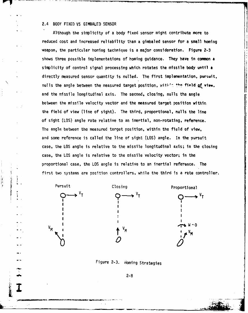
2.4 BODY FIXED VS GIMBALED SENSOR

Although the simplicity of a body fixed sensor might contribute more to

reduced cost and increased reliability than a gimbaled sensor for a small homing

weapon, the particular homing technique is a major consideration. Figure 2-3

shows three possible implementations of homing guidance. They have in conmmon a

simplicity of control signal processing which rotates the missile body until a

directly measured sensor quantity is nulled. The first implementation, pursuit,

nulls the angle between the measured target position, witI'-.-, 4..& fiemid g4 view,h

and the missile longitudinal axis. The second, closing, nulls the angle

between the missile velocity vector and the measured target position within

the field of view (line of sight). The third, proportional, nulls the line

of sight (LOS) angle rate relative to an inertial, non-rotating, reference.

The angle between the measured target position, within the field of view,

and some reference is called the line of sight (LOS) angle. In the pursuit

case, the LOS angle is relative to the missile longitudinal axis; in the closing

case, the LOS angle is relative to the miissile velocity vector; in the

proportional case, the LOS angle is relative to an inertial reference. The

first two systems are position controllers, while the third is a rate controller.

Pursuit Closing Proportional

VT4VT C -. VT

V - 0

VM tM!

Figure 2-3. Homing Strategies

2-8

Pursuit guidance, shown at the left of Figure 2-3, is the simplest; the

output of the sensor is connected to the control loop. However, a problem

arises with pursuit guidance; as the body is rotated to null the LOS angle

relative to the longitudinal axis, the missile velocity vector is lagging

behind. Figure 2-3 shows the missile pointed at the target but the missile is

still moving along its velocity vector, VM In general, changes in the velocity

vector will lag changes in the line of sight angle. Acceptable miss distance

is possible only With low target crossing velocities and practically no

acceleration. Even with a fixed target, unintended missile acceleration mustbe minimized. Gravitational acceleration might be avoided by a terminal

trajectory that is very close to vertical. Otherwise, it must be compensated

by reference to a vertical gyro for instance. Another source of acceleration

V which might limit accuracy is th- ý,,adient of wind speed with altitude.

The targets of interest are expected to have accelerations of about 0.2g when

following curved roads. Therefore, a more effective control must be implemented.

1. fixedThe second of the three guidance methods appears most effective for a

fxdsensor. Although lacking a standard designation, it is referred to as

closing guidance for the sake of discussion. This is mechanized in some bomb

laser kits. The velocity reference is obtained by putting the sensor in a wind

Ivane pod ahead of the bomb. If such a pivoted device is not practical for a

projectile, alternate techniques could be used to provide the velocity reference.

1 Closing guidance is less demanding on the imaging sensor for a fixed sensor

configuration than proportional guidance. Closing guidance is more demanding

I ~for a fixed sensor configuration than a gimbaled sensor configuration. Inj

m order to accommodate the missile body motion, a wider field of view and

accorate LOS must be provided for closing guidance.

2-9

MO&

Proportional guidance is quite effective and is employed in most homing

weapons. By nulling the rate of the LOS to a constant velocity target, the

missile travels to the intercept point in a straight line. The miss distance

from an accelerating target can approach zero. A gimbaled seeker for pro-

portional guidance need not measure angle and can have sizeable bias and scale

factor errors for rate measurement. Proportional guidance places the highest

demands on a body fixed sensor. A body fixed sensor must provide successive

angle measurements from which the LOS rate relative to the body is computed.

The body rate, which has several times the magnitude of the LOS rate, must

be measured gyroscopically (star tracker is impractical) and added to obtain

the LOS rate. This mechanization requires the seeker to make angle measurements

with high accuracy and low noise at a high sample rate.

In sunmmary, we have described three homing methods and the inclusion of

budy fixed and gimbaled sensors. Pursuit guidance is the simplest to

implement with a body fixed sensor but it has difficulty with accelerating

targets and crossing targets. Closing guidance is more effective than

pursuit guidance but it places more demands on the body fixed sensor for a

wider field of view and more accurate angle measurements. Closing guidance

appears to be a logical first choice for application of the second generation

FLIR's to homing applications. For conventional FLURS, proportional guidance,

with gimbaled sensors, is still the favored appraoch. A major problem in

using proportional guidance with a body fixed sensor is that of obtaining

target position relative to the missile velocity vector, so that lead angles

can be developed.

- . 2-10

1__ _ _ __ ___ _ _ _ _

3.0 INTELLIGENT HOMING

There are a number of issues and related work which must be addressed

in the development of intelligent homing beofre we proceed with the processing

of images from the NV&EOL data set. Section 2.0 was developed to provide a

systems scenario for these issues.

3.1 RELATED WORK

Referring to Figure 2-2, we note t:,it to achieve a maneuver footprint

of 600 meters and given a maximum turning rate for our assumed weapon, the

maximum detection and classification ranges are 2.7 km and 1.6 km respectively.

The required search field is 140. If the weapon steers straight in to 1.6 kni,

i.e. does nit initiate steering on some target, the ground coverage will be

reduced 40 percent to 360 meters. !f one second is allowed for classification,

then steering on the target will commence at 1.i km and the effective ground

range is reduced again to approximately 248 meters. Hence, following this

scenario, the ground coverage has been reduced by 41 percent and more weapons

are required to increase the ground coverage towurd the required amount.

Unfortunately, the increase in number nf weapons is non-linear because of thf!

statistics of ballistics dispersion. There are several complementary approaches

fillowed by the services to overcome this problem. i

One approach is the development and fabrication of a high density focal'

plane array FLIk: one estin. te iiuicates that 2-3 km ; an achievable

recognition range. With this device, recognition cruld occur at 2.7 km or

longer (Figure 2-2) and thus allow the required 600 meters of ground coverage.

A second approach is the Advanced Pattern Matching Program of NV&EOL

which requires the incoi,,/ng weapon to pattern match on the background of "fresh"

reconnaissance data, and steer the weapon into a "basket". In terms of Figure

2-2, we define the basket to be 1.6 km from the tar4et and centered on the

3-1

. ..-

7 target.. Thus as the weapon closes to 1.1 kin, and as it performs classification,

the target is still within the coverage. Hence, for this example, the pattern

matching algorithms would reduce the ballistic uncertainty from 600 to 248 meters.

Both of these approaches, defined in terms of Figure 2-2, would allow the

weapon to begin classification at or longer than 1.6 km from the target. We

now describe an approach which would allow the weapon to begin steering on

the target during the detection phase. This approach is complementary to the

above two programs.

* ~3.2 F~XTENDING.GROUND COVERAGE

As ca,- be seen from Figure 2-2, the ground coverage is maximized if target

steering can be initiated during the detection phase, i.e., from 2.7 to 1.6 km.

These numbers represent our model weapon. With a Focal Plane Array FLIR

and use of the Advanced Pattern Matching techniques these numbers would be

extended, with a consequent increase. However, there would still be a detection

phase, and further increased ground coverage could be achieved if target steering

were initiated during the detection phase.At 2.7 km from the target, (Figure 2-2) detections are generated. Under theI

condition of a massive armor attack, described in Section 2.0, a number of

detections will be found in the field of view. Some of these detections will be

target detections, others will be false alarms. Of the latter, there are two

general types: (1) those that persist, and (2) those that do not. Under a

persistence criterion, alluded to i~n the Second Quarterly (Section 1.1), the

latter category of false alarms can be virtually eliminated, in our experience.

Th's is because, in closing from detection to classification range, there are

13 frames, 6 cued frames per second, of detections to correlate cued-frame

to cued-frame.

3-2

In addition, there is the possibility of target prioritization based on

motion. Since we assumed anmassive armor attack, it Is likely that the targets

are moving. Furthermore, the attacking vehicles are probably not going to stop

L • even when they come under a counter-attack. The 13 frames, collected over the

2.2 seconds from detection to classification, can be registered, processed for

change detection, and for kurtosis. This might allow the weapon to discriminate

between moving vehicles and tho•,, which have already been hit and are stationary.

14 At maximum cross track velocity, a tank could travel 120 pixels during the 2.2

seconds, hence chdnge detection is viable. False alarms then would comprise

those detections which do not persist, or if they do persist, do not have

significant motion with respect to other detections within the field of view.

the possibility of beginning target steering at the detection range

J• o rests on techniques such as change detection, cueing, and kurtosis - histogram

analysis which we have already developed in the intelligent tracking phase

of this work. We now consider another important aspect of intelligent homing,

d. ~namely aimpoint selection.I

3.3 AIMPOINT SELECTIONI

Aimpoint -election has to do with selecting a point on the target at

which to aim. This is important for several reasons. There may be a particular-

ly vulnerable portion of the target, the weapon may have a limited capability

warhead which requires more accurate aiming, and the weapon steering may

require thfý selection of a particular limited area of the target to preventI

the steering system from oscillating about the target. The aimpoint discussion

V is broken down into two parts: (I) aimpoint selection based on exterior

* features, and (2) aimpoint selection based on interior features.

I

3-3

_ _ _I

I

3.3.1 Exterior Based Aimpoint Selection FThe exterior based aimpoint selectio,o pco.ess is based on simple moment

measurements of the binary pattern that is ptoduced by the frams-to-frame

tracker. Use of a binary representati,)n i.• ne of the reasons we went to some

lengths to demonstrate the tracking capability of the cuer-binary tracker

combination. Pixels representing the target are replaced with an array of

logical "1"'s; all other pixels are zeroed. Necessary inputs to the aimpoint

selector are target class and aspect. At this point we refer to the discussion

of Section 2.0 and place these two requirements within that context.

Aimpoint selection depends on classification which may be achieved at

1.6 km from the target, according to Section 2.0. Classification could occur

at longer ranges based on a higher resolution sensor and/or a higher signal to

noise ratio. Further, for moving targets the location of the engine hot spot

and the direction of target motion can aid classification at longer ranges.

It may be possible to quantify the reliability of a classification at longer

range based on the particular features employed and the persistence of a

particular classification. In the case of low probability classification;-

steering on the group envelope seems an appropriate strategy. Since the

intelligent homing system includes a cuer, classification will occur as soon

as the cuer makes a classification. Aspect determination is not necessarily

an output of classification.

Consider a simple case where the cuer has classified a target and is

heading directly for the target. That is, the azimuth angle between the weapon

* .and target is zero. The problem is to determine the target aspect, Consider a

tank moving left to right across the field of view. The hot engine produces a

bright spot on the target, so the rear of the target is identified. If the

slopes of the target edges, measured in the image plane, are 900 and 00, the

target is aligned with the sides of the im&ge. If the slopes are 1200 and 300,

"3-4

-L'*'*~

01then the target is rotated 300 in the image plane. Thus the slopes of the target

edges give an approximate idea of the rotation of the target in the image plane.

Length to height ratios also impart information with regard to the target rotation

in a plane containing the line of sight; and parallel to the target ground plane;

this plane is perpendicular to the plane of the image. This approach has some

value in weapons such as Copperhead and Hellfire which are roll stabilized and

either the roll or roll rate is known to a few degrees. For the missiles which

are not roll-stabilized e.g. the longer range strategic weapons, the trajectory

and their terminal "baskets" are such that they are coming in almost vertically

and a top view of the target is presented. It should be mentioned that these

vertical ballistic trajectories present problems under conditions of low cloud

cover. We will present examples of aspect determination in Section 4.0.

b Prior to the mission, the aimpoint is determined by analyzing the target's

vulnerable area for the most likely mission scenario. Once determined, the aim-

point informa tion is stored in terms of a feature vector, F, for each class of

target , and for several aspects. During the mission, a target is detected,

classified, and its aspect determined. The aspect data are used to select a

feature vector from memory for that class of target and an aimpoint is computed

on the actual target to be hit.

The feature vector is constructed by forming a silhouette of the target

for a typical aspect angle. Here the silhouettes can be divided between those

typically seen by a low-flying, roll stabilized weapon and those top views

seen by a ballistic weapon with a near vertical descent.

Referring to the former, Figure 3-1 shows principal pattern axis drawn on

a tank and a desired aimpoint selected. The offsets of the aimpoint from the

four intersections of the target with the principal axes (Rl-R4) as well as the

perpendicular offsets from the pattern centroid (RO) define the aimpoint. These

offsets, along with the major axes of the pattern, define the feature vector.

3-5

Ij A

Y PATrI'rFN AXIS

DESIRE'D'MPACT

POINT

6z. -- PATTERN

SRZY RR R_, ___ _ A

I " I\ ! X .

II•3 !

I:I= (SZX, SZY, al, b2 , a3 , b4 , x Py)

Figure 3-). Aimpoint Specification

-j 3-6

I••;' - ... -k'a. **i • ;'I' 1..•

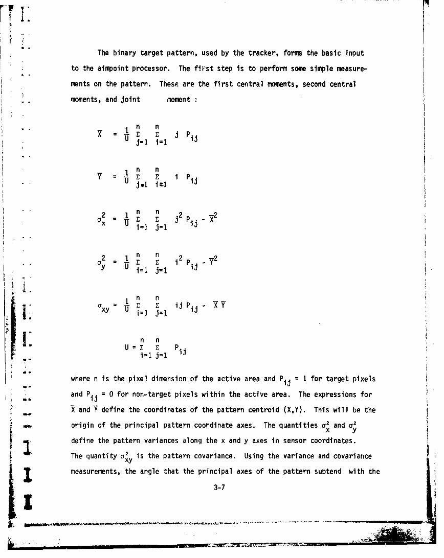
The binary target pattern, used by the tracker, forms the basic input

to the aimpoint processor. The first step is to perform some simple measure-

ments on the pattern. These are the first central moments, second central

moments, and Joint moment

- In nX~ -E•" • J PI

j=1 i--

Sn nY -- £ E E i P.U ij61 i1 i

in n

2 1 n 2

I.x u - £ i -i=1 j=1 ii

2 1 n n 2 ¥Il U i=l j=Z PiJ

n n" ~ ~axy U . ii PiJ"XY

Sn n

U Pi=1 j=1

K -~where n is the pixel dimension of the active area and Pij = 1 for target pixels

and P. = 0 for non-target pixels within the active area. The expressions for

X and V define the coordinates of the pattern centroid (X,Y). This will be the

Sorigin of the principal pattern coordinate axes. The quantities a2 and a2x y

define the pattern variances along the x and y axes in sensor coordinates.The quantity a2 is the pattern covariance. Using the variance and covariance

measurements, the angle that the principal axes of the pattern subtend with the

SI3-7

Iy ....

VI

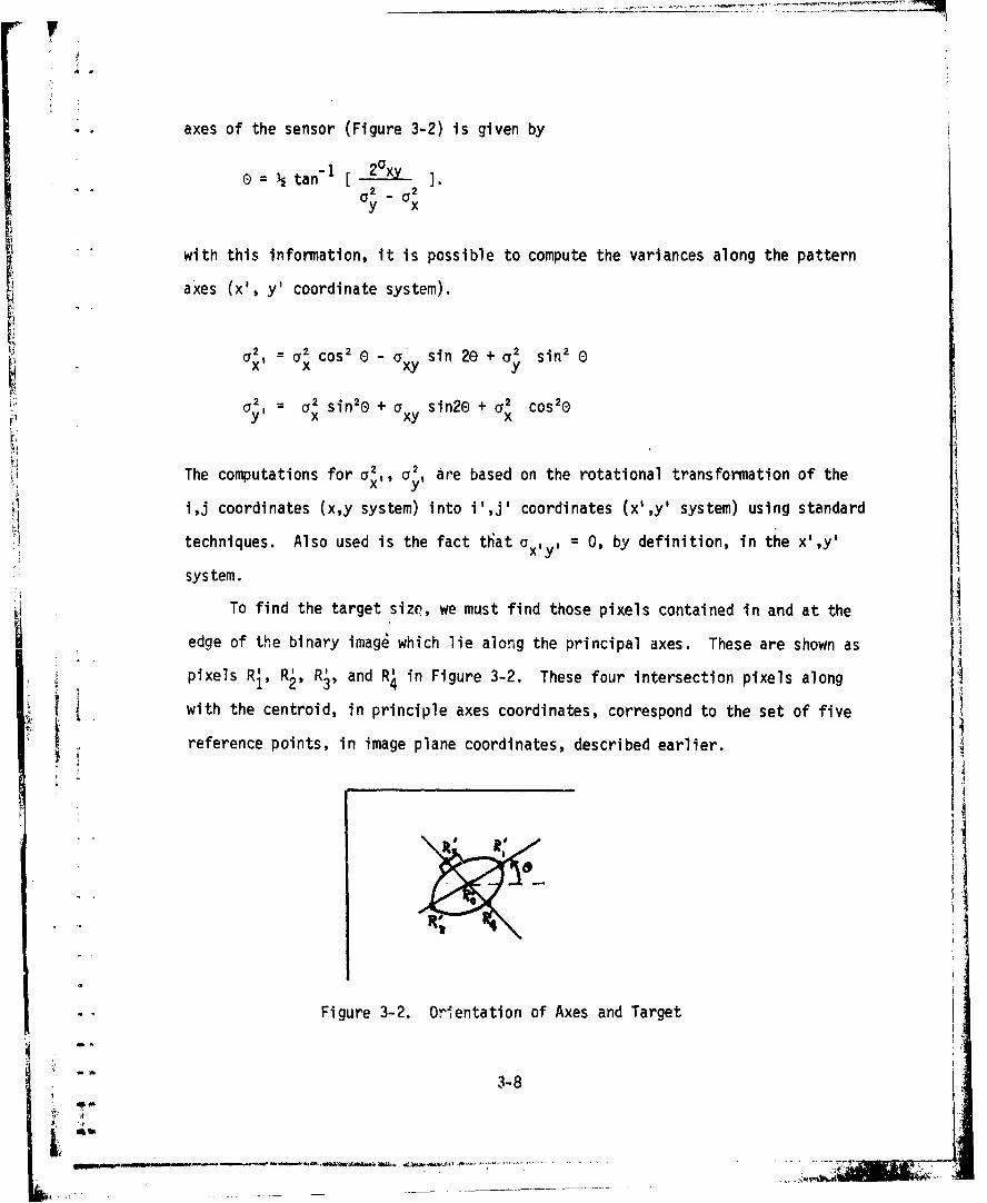
* . axes of the sensor (Figure 3-2) is given by

1tan- 20xy

2 2

y x

"with this information, it is possible to compute the variances along the pattern

axes (x', y' coordinate system).

2 2 2 *= x2 cos2 0- ( sin 20 + sin2 E

2 2 sin2 + sin2o + 2 cos 20P y; x xy X

The computations for ax,, Is, are based on the rotational transformation of thex y

i~j coordinates (x,y system) into i',JI coordinates (x',y' system) using standard

techniques. Also used is the fact tIiat axly, = 0, by definition, in the x',y'

system.

To find the target size, we must find those pixels contained in and at the

edge of the binary image which lie along the principal axes. These are shown as

pixels R R•, Rý, and Rý in Figure 3-2. These four intersection pixels along

with the centroid, in principle axes coordinates, correspond to the set of five

reference points, in image plane coordinates, described earlier.

Figure 3-2. Orientation of Axes and Target

ii 3-8

- "

-

Size ratios are computed as the ratio of the measured size (SZX', SZY')

for the current pattern to the stored sizes in the feature vector F: iRS$X= SZX'IF(1)

RSY= SZY'/F(2), 4

where SZX' = IRI - R;l and SZY' =IR - R41 in the current pattern and F(1)

IR1 - R3 1, F(2) : 1R2 - R4 1 represent the reference pattern.

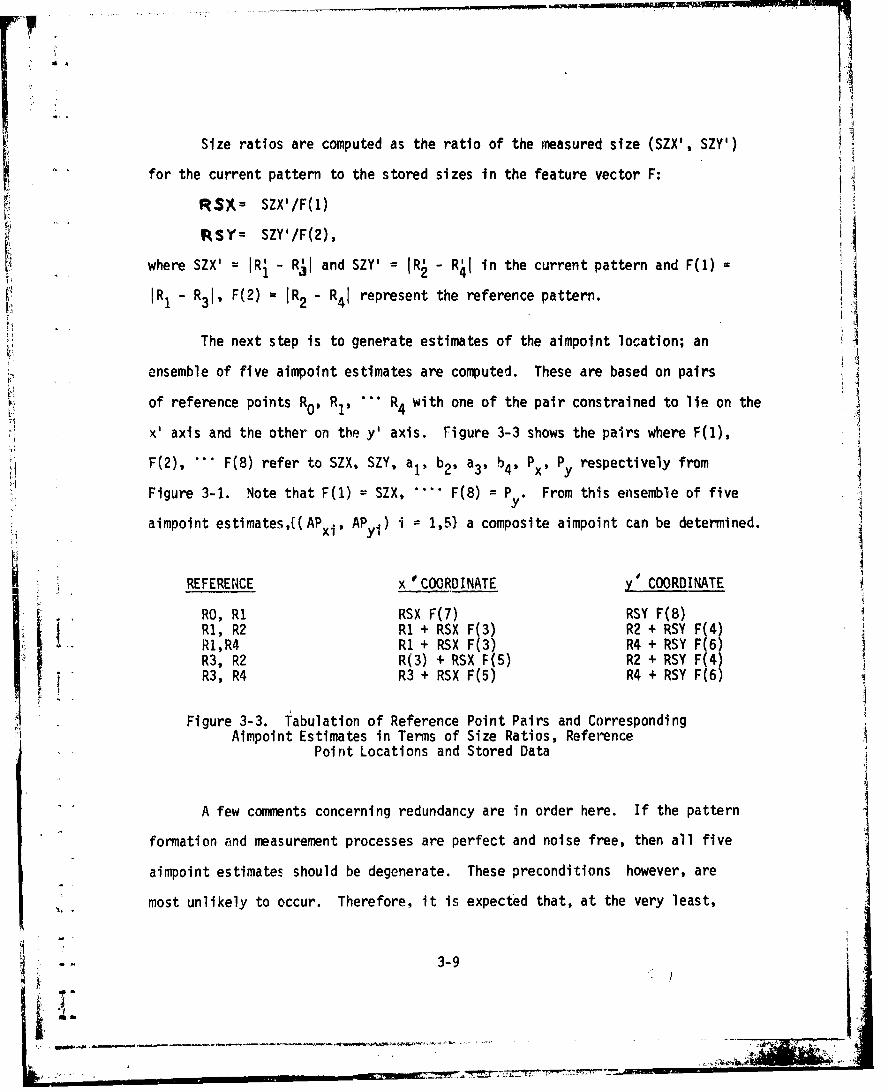
The next step is to generate estimates of the aimpoint location; an

ensemble of five aimpoint estimates are computed. These are based on pairs

of reference points Ro, R, R with one of the pair constrained to lie on the

x axis and the other on the y' axis. Figure 3-3 shows the pairs where F(1),

F(2), F(8) refer to SZX, SZY, aI, b2 , a3, b4, P x Py respectively from

Figure 3-1. Note that F(1) = SZX, *- F(8) = P . From this ensemble of fivey

aimpoint estimates,{(APxi, AP -) i = 1,51 a composite aimpoint can be determined.

REFERENCE x *COORDINATE y. COORDINATE

RO, RI RSX F(7) RSY F(8)RI, R2 R1 + RSX F(3) R2 + RSY F(4)

• - R1,R4 RI + RSX F(3) R4 + RSY F(6)R3, R2 R(3) + RSX F(5) R2 + RSY F(4)R3, R4 R3 + RSX F(5) R4 + RSY F(6)

Figure 3-3. Fabulation of Reference Point Pairs and Corresponding arAimpoint Estimates in Terms of Size Ratios, Reference

Point Locations and Stored Data

A few comments concerning redundancy are in order here. If the pattern ]formation and measurement processes are perfect and noise free, then all five

aimpoint estimates should be degenerate. These preconditions however, are

most unlikely to occur. Therefore, it is expected that, at the very least,

3 -9

S-. -9 i"~'

two or more estimates will be different. The aimpoint ensemble may be thought

of as defining an area on the target pattern. A ;omposite aimpoint can be

computed as the arithmetic or weighted mean over the ensemble. Before this

is done, a simple test for ensemble members is to determine if they lie within

the binary pattern. It should be noted that the RSX and RSY allow the aimpoint

estimate to be updated with decreasing range.

"As the range closes, the target becomes larger and larger and the

tracker must handle a larger and larger track window. Preliminary estimates

seem to indicate that a 64x64 pixel window will require special computation

procedures which take more time and yield results which are not as reli )le as

those achieved with the more straight-forward computa'ions for smaller windows.

Hence, based on limitations of the frame-to-frame tracker, a 64 pixel target

appears as a natural transition to aimpoint selection based on interior features.

3.3.2 Interior Based Aimpoint Selection

Based on the analysis of Section 2.0, and the above constraint, the

rznge has closed to approximately 200 meters (for target side view) when the

* (aimpoint selection technique switches from exterior to interior features. At

500 meters/second, the time to impact is 0.4 sec and 12 frames of data are

available. At 27 meters from the target, the target image fills the field of

view.

An issue here is that range at which the intelligent homing system is

constrained to concentrate on only one target. Again from Section 2.0, we

note that the guidance settling occurs in the last 500 meters to the target.

In the region from 1.6 km to 0.5 km, the intelligent homing system can track

all the targets within the field of view and must commit itself to the highest

priority one before the 500 meter mark is passed. Consider now some character-

istics of the aimpoint based on interior features.

3-10I -P

"Clearly, the aimpoint should represent some vulnerable area. From the

standpoint of image processing, the aimpoint should be a high contrast region

with regard to the rest of the target. It should be repeatable from frame-to-

frame and not scintillate or fluctuate.

In conclusion, we feel that the interior aimpoint selection problem is

not one of identifying the desired point out of context. Rather, the target

has been classifed, the aspect has been determined, and an aimpoint based on

exterior features selected. The aimpoint selection based on interior features

should be in approximately the same location as the former and more time will

K be allotted for the calculation. That is, from 500 meters until 27 meters

to impact, the entire field of view need not be processed.

3-1

2 •

! :i: ,, a-I

t 1 - =.'".. ..... -'"--•"'•• • ' ' " ... •.......

4.0 PRELIMINARY RESULTS

This section is divided into two parts: (1) long range aimpoint selection

and homing, and (2) close-in aimpoint selection and homing. Further, the transition

region between the two and the reasons for the dichotomy are discussed. Three

examples from the NV&EOL data base are presented.

4.1 LONG RANGE AIMPOINT SELECTIONI

Long range aimpoint selection is based on the technique described in Section

3.3.1, Exterior Aimpoint Selection. At long range, the exterior shape is a

reliable and repeatable feature. This section provides an example of long range

aimpoint selection taken from the NV&EOL data base described in the First

Quarterly Report. Section 2.2.5, Tape #5, 11/15/77, Tape Position 5280 is a

side view of a tank moving perpendicularly to the field of view from right to left.

The median filter was deleted in this example only because we were looking

for a small engine hot spot in the segmentation process. Hence, the aimpointselection and tracking are based on the binary values resulting from the

segmentation processes described in previous quarterlies with the deletion of

the 3x3 median filter for this example only. The model for the aimpoint selection

It is shown in Figure 4.1-ia.

In Figure 4.1-1b, we have arbitrarily assigned values to each of the eight

members of the feature vector. We place the coordinate system at R0 and the

directions along the principal axis are the same as the sensor coordinate system:

i.e, down is positive and left to right is positive as shown in Figure 4.1-1a.

In this coordinate system, R3 and R2 have negative coordinates (-x',O) and (0,-y')

respectively, while RI and R4 have positive coordinates. Figure 4.1-1b shows the

quantities for the reference vector; note that some of the quantities are signed

values indicating direction. The aimpoint is labelled AP and shown with an

asterisk (*)

4-1

I-I~' ~ i.-

ItII

a. 1

SI

Figure 4.1-1a. Principal Axes Directions.

FEATURE VECTOR

F(1) = SZX = 4F(2) = SZY = 3F(3) = a1 = +1

F(4) = b2 = +2SF(5) = a 3 - -3 iF(6) = b = -1F(7) = e = -1

SF(8) = Py = -. 5

Figure 4.1-1b. Reference Quantities

The following figures show the binary target shape from the frame-to-frame tracker,

described in Section 1.0 and previous Quarterlies, for consecutive images

224, 228, 232, 236, 240, 244, 248, 252, 256, and 260. The aimpoint calculations

are shown below each shape and the aimpoint is superimposed on the target

silhouette. We describe the aimpoint computation for image 224 in some detail

4-2

|- -

•,.2

i

and then present the remainder of the images and their aimpoint computations.

Image 224 is shown in Figure 4.1-2. The first and second central moments are:

n n

XBAR J PjU J+l -1 ii

n

1YrYBAR U i PipJul 1=1

n nwhere U = Pt. and i and J are the row and column numbers starting from

i=1 Jui

the upper left-hand corner of the track window. The first central moment is

computer on a binary image by summing the number of "1" pixels in each column

and multiplying by the column number. These products are then summed and

divided by the number of "1" pixels in the image. Thus,

f=XBAR = -- [10x6 + 11x6 + 12x9 + 13x9 + ]. = 17.78 and,156"'

Y=YBAR = 1-'[6x6 + 7x4 + 8x12 + 9x14 + ... ] 1888/156 12.10. The

variances,

S( 2 = I n n tu'

a • J - (XBAR)li=1 j=l

1na;2 UZ E i2 -ij (YBAR)2

i=I J=1 Pi

can be evaluated in a similar fashion as well as the expression for the Joint

moment, a. The XBAR, YVAR pixel truncated to (17, 12) is shown circled in

Figure 4.1-2. We note that a ,y provide a rough measure of the target extent

in the x,y directions as measured by the coordinates of the image plane. The

angle that the principle axis makes with the image coordinate system Is found

4-3

iVI

A I P P N T D I P L A Y, ,, OOO..ll, .. 0 O 0 O • •@ OIOSO 00" *" °

o*s*e, eo...o~oooe o..***o*o****AR =R 1 R782ooo,,,,,,o. 1Ll/,, L1, ,, ,,,,YHAR = 12e103o. .,o0. ,oo JooSIG2X = 18,094

o,,o,,, , 1 1t 1111o,,66 * So 'I G 2 Y = 94 -19eo ,,o. 11J.L IL11 t11100666 S oT oG X •IY le1227

.,o...,L111 11'11110060.o. THETA -7.907o,..,..ll.�.. • •SIG2XP = l8.264

a. *,..,.. 111 1 ,libo...... Sn2YP =55

.. ,.°.....******... lt.11 1L1 1 o,,o AIR? P1 O 7.. o.1-R3 - 210 11

o.o...o,..S. 111111. o- R,4- 17 17oo.,.o°,oeeeoe .. o. .o....*-** -o - AIM POINTS

S-3.790 1.66?

-3.790 1 a66 TS.,.*........o..... o.. ,oo.** ,..* -3.790 1.66"

..... o..*.oo....o..-.-. .- ..... ....... :...***.................:1.. 1.

Figure 4.1-2. Image 224 and Aimpoint Computations

by substituting into

E) = tan l [ _ x ] tan'l 1 [.20yt- x = (9.425-18.094)

and= g00 =-7.9°

Thus by a rotation,

x' = x cos0 - ysin E

y = -x sin 0 + y cosO,

a point along the image plane axes can be mapped into a point along the principal

axevs. The coordinates of the perimeter points along the prircipal axes can be

found from this equation. In fact, all four perimeter pointsV-are shown in

Figuire 4.1-2 as t:ircled pixels along the principal axis. In order not to clutter

Figures 401-2, the perimeter points R1, R2, R 3 , and R4 are snown in Figure 4.1-3

with Rb, the centroid. These pixels correspond to those of the. model target

shown in Figure 4.1-1a.S4-4

Figure 4.1-3. Location of Principal Axis-Perimeter Pixels

The next step is to determine the size of the actual target with respect

to that of the model. In hydrodynamic modelling, this is the constant of

proportionality. From the actual target, image 224, SZX' = JR! - R31 and0I

SZY' =4 - RAI

SZX' = [ (23-10)2 + (13-11)2 ]½ = 13.2

SZY' = [ (18-17)2 + (17-7)2 ]½ = 10.1,

* and the model target has SZX = 4, SZY 2 3. Hence the constants of proportion-

ality are RSX = SZX'/F(]), RSY = SZY'/F(2) which becomes 3.25 and 3.3, respect-

ively.

Now, we compute five estimates for the aimpoint based on various combinations

of RO, R1, R2b R3, and R4. The five sets of coordinate expressions are described

in Section 3.3.2 and the dppropriate numbers for this example are shown in

Figure 4.1-4. Note that the aimpoint coordinates are referenced to the target

centroid, but they are measured along the x,y axis centered at the centroid instead

of the x', y' axis for the illustrations.

-4-5

REFERENCE X` COORD Y' COORD

RO, R1 RSX, F(7) - 3.25 x -1 RSY • F(8) a 3.3 x 0.5

R1, R2 R1 + RSX F(5) 6 + 3.25 x (-3) R2 + RSY * F(6) +5 +3.3 x (-1)2 2

R1 , R4 R1 + RSX * F(5) - 6 + 3.25 x (-3) R4 + RSY - F(4) * .5 + (3.3) x (+2)

R3, R2 R3 + RSX • F(7) - -7 + 3.25 x (+1) R2 + RSY * F(6) -+5 +3.3 x (-1

R3, R4 R3 + RSX " F(7) - -7 + 3.25 x (+1) R4 + RSY " F(4) * .5 + (3.3) x (+2)

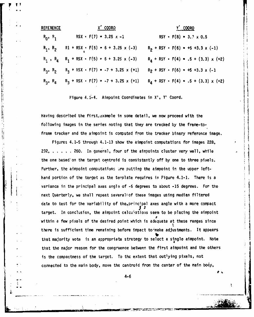
Figure 4.1-4. Aimpoint Coordinates in X', Y' Coord.

Having described the firsttexample in some detail, we now proceed with the

following images in the series noting that they are tracked by the frame-to-

frame tracker and the aimpoint is computed from the tracker binary reference image.

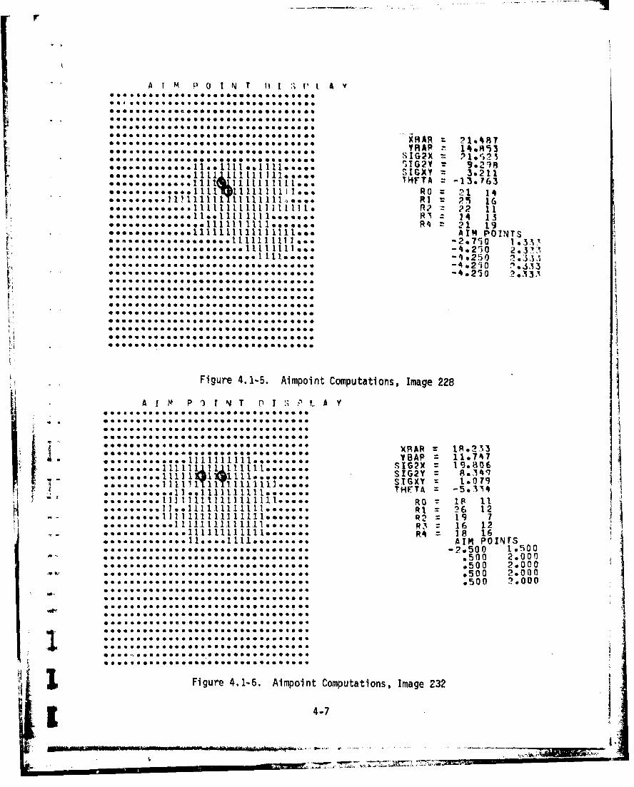
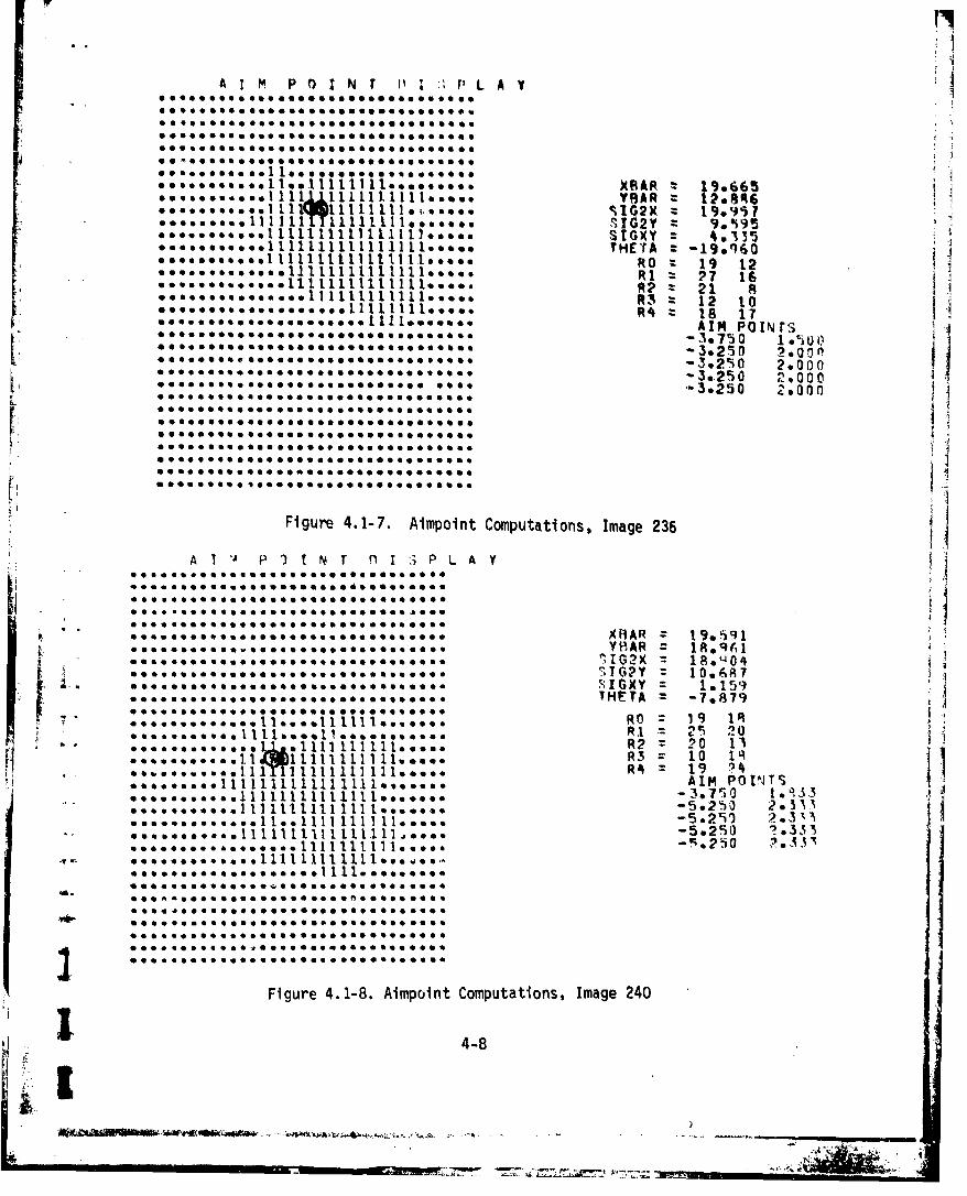
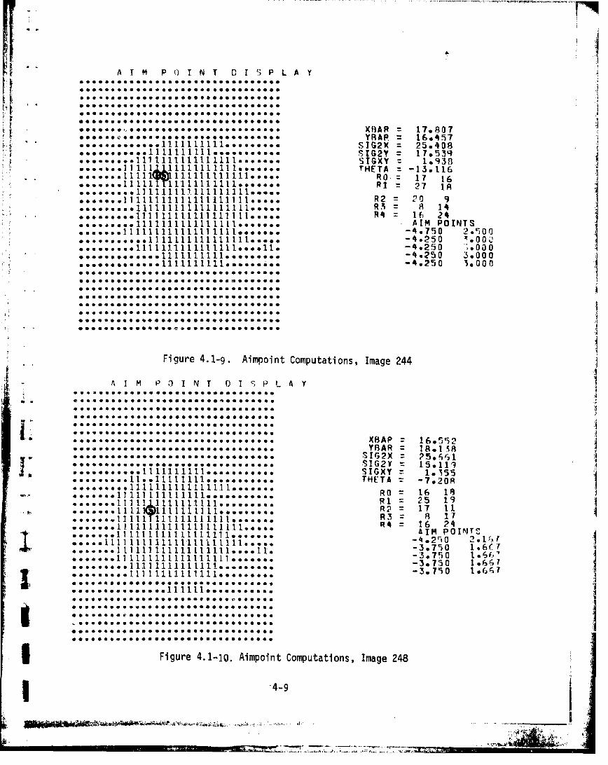
Figures 4.1-5 through 4.1-13 show the aimpoint computations for images 228,

232, ..... 260. In general, four of the aimpoints cluster very well, while

the one based'on the target centroid is consistently off by one to three pixels.

Further, the aimpoint computations Are putting the aimpoint in the upper left-

hand portion of the target as the template requires in Figure 4.1-1. There is a

variance in the principal axes angl4 of -6 degrees to about -15 degrees. For the

next Quarterly, we shall repeat severalsof these images using median filtered

data to test for the variability of thepr'incipal axes angle with a more compact

target. In conclusion, the aimpoint calcu',atfons seem to be placing the aimpoint

within a few pixels of the desired point which is adequate at these ranges since

there is sufficient time remaining before impact to'make adjustments. It appears

that majority vote is an appropriate strategy to select a single aimpoint. Note

that the major reason for the congruence between the first aimpoint and the others

is the compactness of the target. To the extent that outlying pixels, not

, * -connected to the main body, move the centroid from the center of the main body,

S Ii 4-6

- 44;

F

A M P I N T ti i :; P L A

Oee.e0@.4. n OOO4056g3geO Og .O0e

ego....o.. .g. .... ooo..ooooo.ooo. Y00 ~ o5"'soee e. Ce..eo. 06 eo. ... s .05.o oo @6• 0 -

SIG2X )I ,1.!1I2Y 921• o. 000 000 011 0111 0.1 11. 0.0SIGXY 30•211Io1H: TA -13063

ogg., 1 1 .. 11 1111111,,00% R. () '. 1

o.... o.g.......t t .1111...4 : 1• .o, o..o.111•ttltttt~ oAIM POINTS

-4.250 2S.'s3"-4.250 i.3333

"-4.250

Figure 4.1-5. Aimpoint Computations, Image 228

*A. I M P ')T 'Y T r.)1 S L~ ?A Y

U*O00S* OOOO°00 0 °eeaOOOOO **OOO° 00

XRAR 1r I 03 3't8AP =11.7 47

GY 19.806STGXY 1.079

11 1 6 41 o e1 1 111 1 11 1 * R I=.6 1

a 00 = 19 76. oe 06 6.o.1 11 1Ih.l.. R 3 =16 12

110..1 11..... *gAIM POIWSO 0 ° O-2.500 1.500

.500 2.000.500 2.000.5 00 120000

+ Figure 4.1-6. Aimp01nt Computations, Image 2328

............ *..P...**T .t00A 41

S- i -ii....-- eg g.*. ** g .g.. **6g..0 geO°. .geg •Oeeeg S

*000116011eg11m. *A***=**115000

+ ~ *g.. @gSS it ttege0 tt00g ttS,.g., + Y= 1.z!

Sa 0 0. -s.-. 11 1.211r... ° R• .. 181.

A M P 0 1 N r & :; P LAY* Q00000**....00000..000.606000. 0

00t0010000.00 I00600000000O006000

e.,o ,,,, ,Ll ~ lll lllt oo., ,,.XPAR = 9e665 i*000u00 .60 9160 000 00 00 11* 1116*00 0A 281

06000004i.0 006 02X 19991100 66 0

S 0o00000 000 00 000t0 0o,, G 2Y .90%95

o - , . , , t o , 1 1 1 1 1 1 1 1 L l l ] , , , ,S I G X Y = 4 1 3 • 5t HET A = -19.95?a1 -o,,,,11111lllt111111,se.°. RO0 % 19 12

Ri =2P 16*oo-ooooo,,,1lll1111111111110o0. RP x 21 R• , ., °°o °. ,, lll ll lll °, ,,R3 x 12 10

R4 B1 17• ....-... o.-.....!...1Iltl....... AIM 18 17

°,°o °°°, ,°o o- ° °ll 1°..o°,AIM POINts00000- 0 oe-,°°,o°,,°°ooe eoo~ooo° -32750 1 f° Un

-3o250 2I 0 0-3.2'S.0 2.000-3L250 2.000

OOO250 39250000 0000O00° O O0000 too00 o°O5000°000

000060O0000006000O0eg O000~OO0600

000060006 O000OO°°O600000000000°OO°

0000000000°°°0O00000600000.0.0O00

O°000°00OO0060*O00°0°000.000.00.0

*00OOO00000°00°0600000°OO000000°O

Figure 4.1-7. Aimpoint Computations, Image 236

A I " P I f N T n I P L AY

0O000000000600000060000000060000

O000060600.06o600006006006600061

O00000o060O°Oe006*000060°000*0°o

""XAR = 19*591*O°OI°OO°OOU 0060000°0°°°O° 00e°° Y•A 0R9

I G2X z 18,904'TGPY = 10.687*00.00.00000000006OO°°000 06 50°°°Yo1.oo9, ;. o .. , , o,. o, °oooo eo°,o - IGXY = 10159THE TA = -7*879

*o .." o°,,.,11.,°olll1o.,oo,. RO = 19 1 AR'l = 21 5: 20*...oio•o lll... 11.o..o~o,. R2 = 20 12

• ,,,ll~l~ll~llllo°°° • :19 14o1 iAIM POINTS

*0 .001111111111111 1.oo Rft 1ý9 1 ?4 3

06000000006llt lllui 111 i . -5s290 '.)333, ., ° 0°.01111111111.600. - ,250 1-3.31.00 o,,,o .o l 111. 1111l 1..°..o000.0 °0 "''°'o600.o111.60000.0.

0 ....00O.....°00111O 1 O000600

000 @-g Oe ° 00 0 0 00 0 f0 0 66600

00Figure 4.1-8. Aimpo0nt Computations, Image 240

4-8

[ Jll 'm 1 -I.~ w o '. I r.. . -____________

"'" I .

A AQie T P0 TNT DI 0m PLAY

0 e 000000 0000* 00 @0000060.@0.. .

.0,....***,oo.*oo.* *XBAR = 17.807YRAP = 16. 497

SIG2X = 25.408 !oSIG2Y = 17o539?S• o.. .oo 111 1t1 111 111 , . ... STGXY .= 1,938

. . 11 1 1 11 1 1 1 ..o. THETA = -13 .1.16

a00,eo° 1] 111 6111111111 o.....

°o° ,., 11 111 111 11 111 1.° .. R2 = P 9• , °, ,o 11 11 11 11 11 11o, .. RA = 8 14

, o . , o ° ~ l l l t l l l l l . ,. o. .. R 4 = I f F )

*0004,061111 11111111 111 1.'... AIM POINTSeo .... . l1111111111111 11110000680 -4.790 2 * 0 0

-4.250 7000Ol . . . I 111 .11 111 *1 oo• * -4.250 0.000., .....•.o•.o 111I1I oI o°°. . o.... ° -4-250 3°000

-4.290 36000

A

Figure 4.1-9. Aimpoint Computations, Image 244

A I M P I•0 1oNT o 1 oPLAY

I. .. ooo..ooo ooooeo0• o..e°oo°0oo o.

... .. .. ......... . ...... . .0e .06e S .* . 0. XfHAP = 16.592YRAR = loot158SI2X= So-S I G2M Y = 5 T I I 1

THETA -7.208!..1"1""""R" ".......... 25 19

•---...1111-11111-1..*.. ..... 00. R = 65 19Sa .......... ..111111111........... A= 17 11.

-3.79 0 1.06( 7*.,,,o1111111111111111.750 1°6oIS . ..... I]Iil111l111111.0........ R -3.790 17

• Io.•. 111111111111111...00o I3= 81... 0 0 0 0 0000.. I I1 11 11 1 11.... ... .. 0a mP It00. .... 0 11111111 1111IIIIII111,...., -I20 2,•

0600 0 a0 a0 a000 0 0 00 a0 0 00 a 0 a0 06 0 a0 a

• . .... ~ 11111 *111 *1111111...0..I'°- ,7 0 1,o0o...* 0 0 ..1 i1 1 11 1 1 1 o .... , -.0750 1,66"

0..... ... 0 *.1.1111...0... ...

Figure 4.1-10. Aimpoint Computations, Image 248

-47-9o

3-2 13. 19 4.~I;~~' II P'XYJ 1018LA8Fe***..**THETA -es7ege 0ee8g 1

*..*.....*.RD 13*.**..19*.

I'll S*.**.*06006666609640 RI =e20 21

XRA 132550

V-@9 3.3S33.)~

-4 25 -3 1 b9 3

Figure 11111 41-11..... Rp n Copuaios 15ge25

OC*~ II11l11*Y =o 195413

jg... R11111 1 27 19.... ..

AIMAI POINTSDISLA00~~o2t 200%16706.0

*~~~~-*5 .o..go'066CO O O00000.. o~o~o-3.750. 2 4, f;6***ef

412 4-1028

the aimpoint will be different. The model for the first aimpoint assumes

that R6 is equidistant from R and R•.

Figure 4.1-14 shows the aimpoint for images 229,228,...260 where

median filtering has produced a more compact target representation.

A IM P1 NT S P L A Y*................................

.........................

WMAR = 13.1152*.............................YNAR z2.7... ... ....... SG =3 3

TH T = -23 174ooQ ee *

S.......................................I 2 12• "* ,1.I..I.12Y 10,.30

........... ... 2

*..1111011111 11111 -400 2.

S:.::::::::::::::::: : 0i2..............1111!1 .. I2e6........................................................1111................... 1 1

0-..11.111.11111!.. . . .. . . . ii .............

..... 111el 1 :3 000 2 .667 ;'

.......... ...............

• ** .]l :•:] l~t~t•........... . 0 • •

• . 111 11 111 1!1 ]! . ........... 3 0 . ?

Figure 4.1 13 Aimpoints Computations, Image 260

Figure 4.1 14. Aimpoint Computations, Images 224,...260

for Median Filtered Images

4-11

Fiur 41 3 imoit Copuaton, .mae.6

_ _ _ _ _ _ _ _ _ ___ _ - 4. ~

i.. . . . .

4.2 Close-In Homing and Aimpoint Selection

The purpose of this section is to discuss several preliminary problems

which must be solved in order to accomplish close-in homing and aimpoint

selection. The first problem is segmentation of a close-in target and the

second is frame-to-frame tracking of such a target.

4.2.1 Close-In Segmentation

Segmentation of a large target, 30 lines or rmore, introduces several

differences from segmentation of a small target. The smaller target can be

segmented as a light target against a dark background or vice versa. A large

target may consist of both light and dark portions; hence, segmentation

techniques for large targets should be bipolar. A second difference is found

in the interior, structural features which are present in the large target.

These features may exhibit the "blob-like" characteristic of a small target,

i.e., there exists a general decrease in gray level as one moves from the

center of the blob to the edge in any direction. Hawever, th,-se features may

also exhibit "contour-like" characteristics, i.e. the gray level does not

diminish isotropically as one moves from the center but may increase in one

direction and diminish in the opposite direction. As an example of close-in

segmentation, we consider images from the NV'!.:OL 875-line data base described ~=

"in the First Quarterly Report. The scenario is described in Section ?.2.5 "Tape

#5 11/14/77", Tape Position 5280. The helicopter is closing on a moving tank

from the rear; the tank is moving along a narrow road. We shall show in this

example that it is possible to segment the target better by moving beyond the

superslice threshold which gives the maximum edge/perimeter matches and consider

-- the kurtosis (texture) ideas derived in the Third Quarterly Peport. This

- allows us to determine target aspect which facilitates aimpoint selection.

Further, by means of the same kurtosis ideas used in the disappearing and

* •4-12! a

i': =I-"-'

reappearing target cases of the Third Quarter,-ly, we can estimate the threshold

at which target background merging occurs.

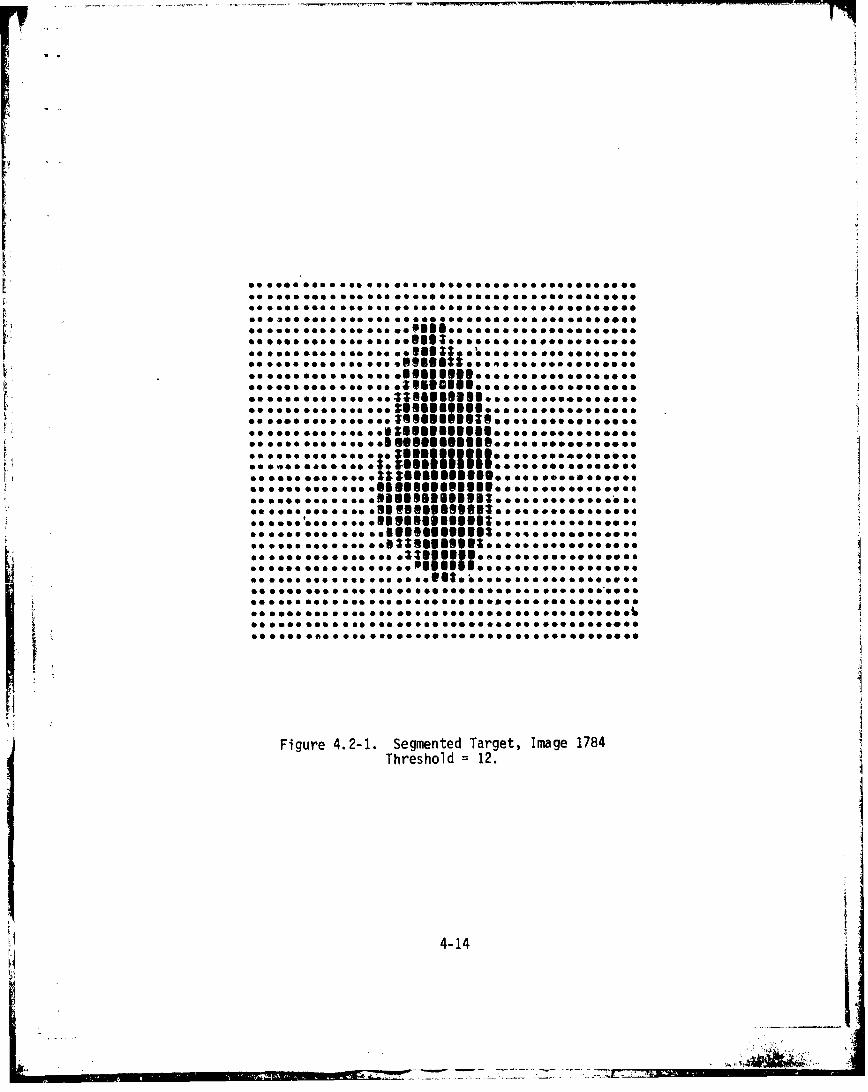
Figure 4.2-1 shows the segmentation for, the tank at a threshold of 12;

essentially, the segmented portion is the hot erigine. Figure 4.2-2 shows the

number of edge/perimiter matches, average graY level, average x position,average y position, width (DELX), height (DEL(),*,total number of pixels, and

number of perimeter points vs. the superslice threshold. Note from the figure

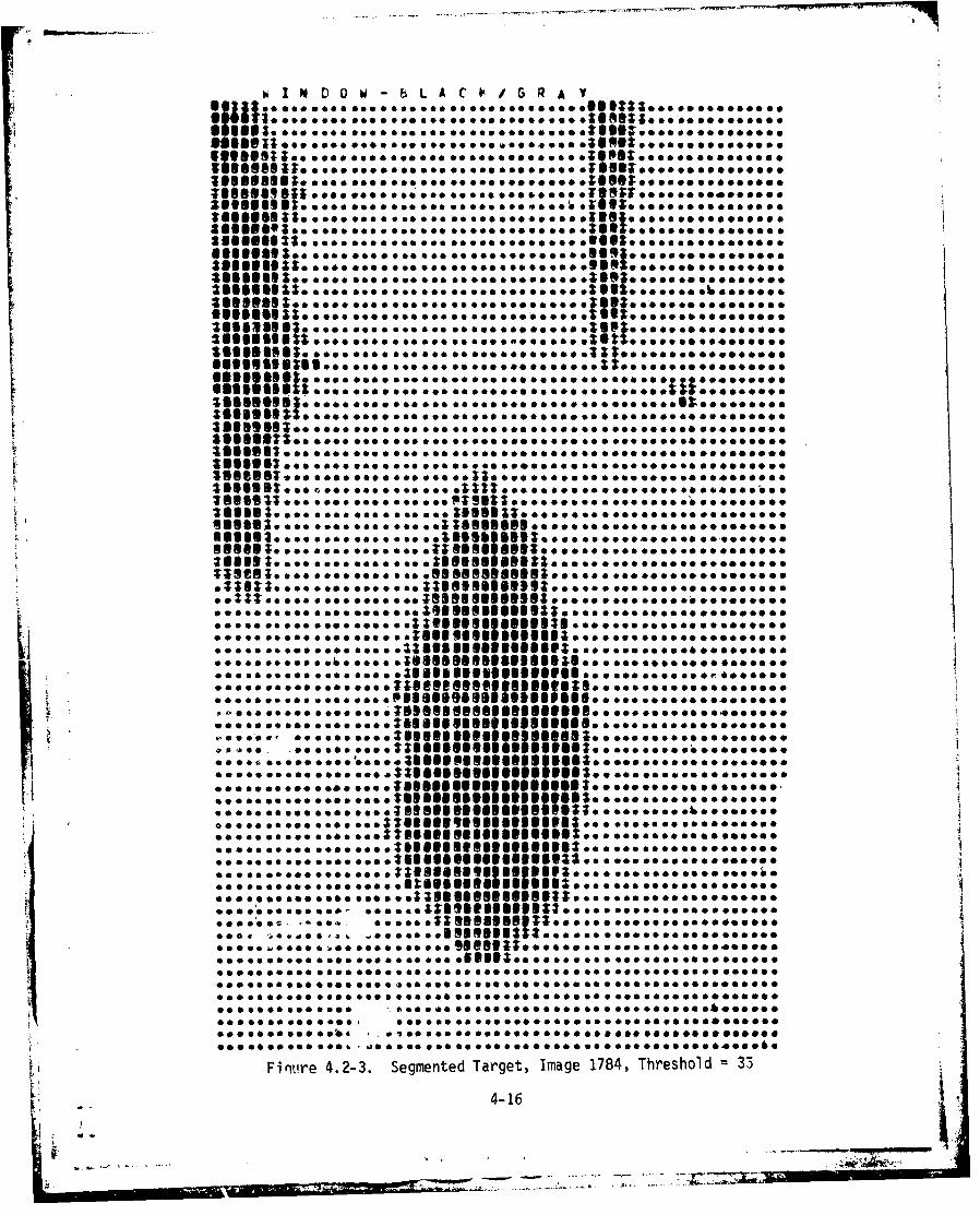
that the maximum number of edge/perimeter matches occurs at a threshold of 35

and that image is shown in Figure 4.2-3. Continuing beyond the threshold for

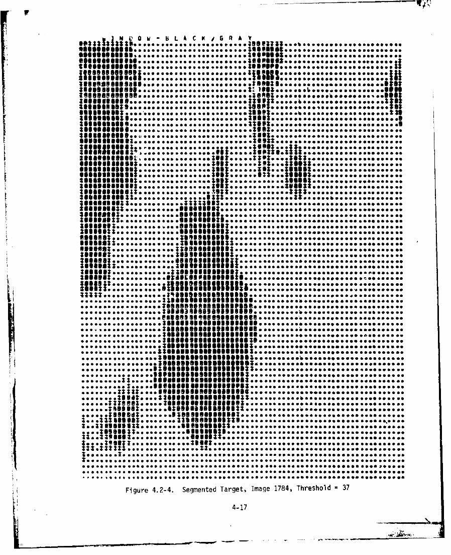
maximum edge/perimeter matches, we obtain Figure 4.2-4 at a threshold of 37.

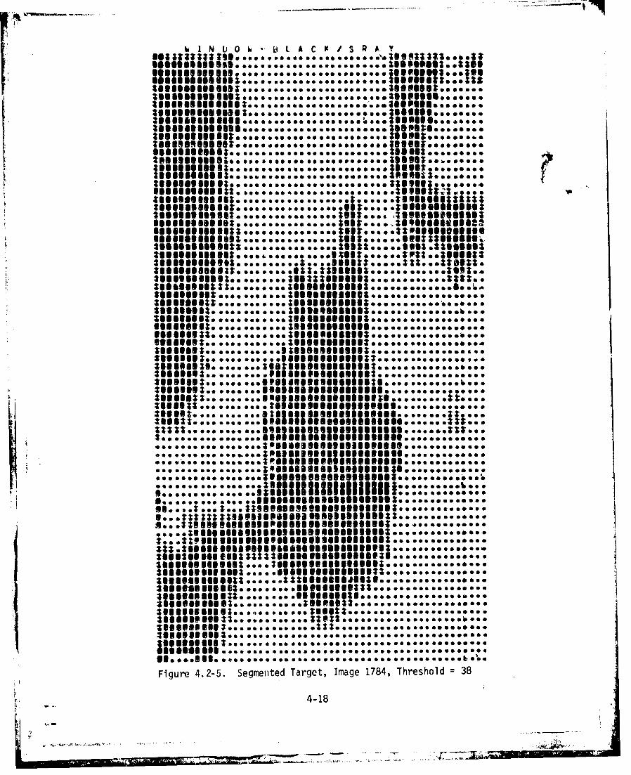
Here, we can see the beginnings of the distinctive gun barrel. Figure 4.2-5

shows the same image, thresholded at 38 and the ensuing merging with the back-

ground. Note the large jump in the number of pixels contained in the target at

a threshold of 38 and the large jump in the average gray level. This jump is

Li similar to the jump in target size for the disappearing target case when the

ji backgournd was included in the target shape. Further, the large expansion in

the target's x dimension leads one to suspect that the additions are not part

of the target. An added degree of sophistication could be achieved by tracking

the background blobs as they form and computing their probability of being part

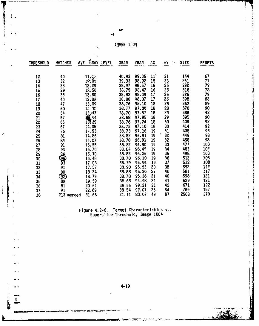
of the target by their additions to the target dimensions. Figure 4.2-6 is the

descriptive table of target characteristics for image 1804. Almost the same

thinq happens again except there are several maximums in 2804. Again, they are

pissed on the way to the best target description.

In conclusion, it is seen that a more complete segmentation of a close-in

Carget can be achieved by taking into account not only the maximum number of

edge/pierimeter matches but the average gray level across the target and the

number of pixels added to the target at each gray level. In the next quarterly,

we hopr to reduce these heuristics to something more concrete based on further

examples.4-13

. . . .4 .. -...

Og Oll 00 000go 99O 0000060 0OO0000O000000000

go sees @00 050 to SoO oe oeO1111 9 060 a* 00664.9 0000

0505 0 05 00 Z0909298019190 0 s &5 00000500

• es....s.. eo. see s.eS3I•esssssoseoooo.esso.oo

oo *o6o 0 00005000 .oo eooooo.oos..eosoooo0 0 o aoo..o o. oo. 09gggg ooo•o*...*.....o

o 0 0.• 0os a 0. •.uoess uus.o o a 0o a 0

boo oo .. s..s.uhmggg0 ogg3.s 0. .. . eoo ..

Figueo 4.2-1. Seegmen T ,•:U. u313....... 1784e so �0001050550•0 505o555 oThreshold 512.

4-1

Figure 4.-.Semne Targetoo ImOagJ~~ooooeo1784o. o•oo .o Threshoo ld l=12. , ,eoooee

o, °o° oo • 0 .l;$llllO~lO~o• o • eoooo o ILI 4-14••ooelJllOl J~ ,•eoe •o

eoeooeeo•oeoN~lJ•JJJJJ|•ooe~eoooeoI.0, oo.00o• •00 80•7I000 h:io o-•o.,,,0

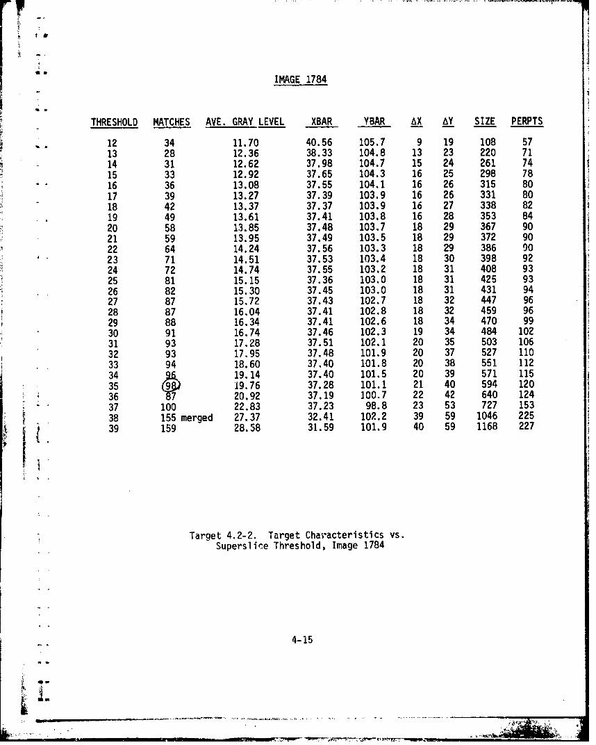
IMAGE 1784

THRESHOLD MATCHES AVE. GRAY LEVEL XBAR YBAR AX AY SIZE PERPTS

-12 34 11.70 40.56 105.7 9 19 108 5713 28 12.36 38.33 104.8 13 23 220 7114 31 12.62 37.98 104.7 15 24 261 7415 33 12.92 37.65 104.3 16 25 298 7816 36 13.08 37.55 104.1 16 26 315 8017 39 13.27 37.39 103.9 16 26 331 8018 42 13.37 37.37 103.9 16 27 338 82

*.19 49 13.61 37.41 103.8 16 28 353 8420 58 13.85 37.48 103.7 18 29 367 9021 59 13.95 37.49 103.5 18 29 372 9022 64 14.24 37.56 103.3 18 29 386 90

*23 71 14.51 37.53 103.4 18 30 398 9224 72 14.74 37.55 103.2 18 31 408 9325 81 15.15 37.36 103.0 18 31 425 93

-26 82 15.30 37.45 103.0 18 31 431 9427 87 15.72 37.43 102.7 18 32 447 9628 87 16.04 37.41 102.8 18 32 459 9629 88 16.34 37.41 102.6 18 34 470 9930 91 16.74 37.46 102.3 19 34 484 10231 93 17.28 37.51 102.1 20 35 503 10632 93 17.95 37.48 101.9 20 37 527 11033 94 18.60 37.40 101.8 20 38 551 11234 9419.14 37.40 101.5 20 39 571 11535 (99 19.76 37.28 101.1 21 40 594 12036 r720.92 37.19 100.7 22 42 640 12437 100 22.83 37.23 98.8 23 53 727 15338 155 merged 27.37 32.41 102.2 39 59 1046 225

394 159 28.58 31.59 101.9 40 59 1168 227

Target 4.2 -2. Target Characteristics vs.Superslice Threshold, Image 1784

4-15

3I6III33~06000000000e000000

sea..0e.s;. .......

*SSSSST*0 oSo*&o o 0 so *oeseo oooebeo*e~oeoe 6 e6*eeoee-0 *SOSOe

em....,00 *Soo....... 000 *so 0600*00e000*0..00.e.*.00*0000100

3s3seso~oeesooooeseve *sess $991o0*00069eo6oeeoe0*oo6ooeeo

00.0 *** C000 ozzleffeulsugso .. e Malto**ses;* **aso.

0*000 .. Go* *s...00*0060000

600060060 .. ;sueeus;..

6000,600*46......40 S91 363...........

000000#0000O00O0* uSSSOSS5U5*0000000O0

6,0000C'00000*6 .ooooo*oooee51656666*oo00000*00000000000000

Figure 4.2-3. Segmented Target,5Image 1784,*Threshold *33

................ 31S55461630355......o..

363ho *so.ee ,s *o o ***s* 9@1131 ooeoooe*ae000000geja

IIt

IDIOM11S111110. Itee.. .... e. ... j0 see.. *a.ee.....see.e

selotes*oe .....*S o. P3.;

300000006 . ..... . .& e...

2111131133.... ~ ~ ~~oo eec.... **bUS~eeg....ee* a&*..e.&so*eC060 .

:uaFigur 4~~. . 2-4.. S Segmnte TaretIm ge174 The shold 37~g ee~g.e

316@313..... 4es17

6 10 m LA C18SM18 coes[*so psse o 00

Iw. so~ 6 se ss*66.0660.68.Mps$ oe ....... tS S I.ZS000488198o **a*

Me@so Mma mesamm 04* 0,0 0*6a o *. 0 *0 a.**..M.10104SS.a.a

29919911169 ese **a* *go*** so 0.ISPBS.....

3sssssssmsg.......as.3:ssmsgz...........gzt.

smsss~uz.... .... . gssss~usca....... . .age.

;Msgsasg..........gssmsmgsasmg....... *a**-*

461100:6 to:::c ::: 0:

:uussss:..006 off. .. asm as@soffs lessee*&* St 00...

000 0060 see

new ottz Sts ttl M spil ai 191118511998125to&*** 666066690

0 0* a31*Zes sl @o.. lines seen... 4 sgloe198as* a seo ae b.e go astoo 3315 51 less@* Metal0 8981946989 so 00s0 *a5 Soso a0lb 00000

Figure 4.2-5. Segmen~ted Target, Image 1784, Threshold =38

4-18

I)

IMAGE 1304

THRESHOLD MATCHES AVE. XiRAY LEVFL XBAR YBAR AX AY ", SIZE PERPTS

12 40 11. 40.93 99.35 11' 21 164 6713 32 X;%0•, 39.33 98.92 15 23 261 7114 28 12.29 38.97 98.57 16 25 292 7915 29 1?.50 38.75 98.47 16 25 316 7816 33 12.60 38.83 98.39 17 25 326 7917 40 12.83 38.86 q8.07 17 26 398 8218 47 13.09 38.76 98.10 18 28 363 8919 50 1ý10 38.77 97.88 18 28 376 9020 54 1,.17 38.70 97.57 18 29 386 9221 57 "5S4 J8.68 97.95 18 29 395 9022 65 1(3'35 38.76 97.24 18 30 405 9223 67 14.05 38.75 97.10 18 30 414 9224 76 14,53 38.73 97.16 19 31 435 9525 81 14.86 38.82 96.91 19 32 449 98

26 84 15.07 38.78 96.91 19 32 458 9827 91 15.55 38.82 96.90 19 33 477 10028 93 15.70 38.84 96.45 19 34 483 10229 16.10 38.83 96.26 19 35 498 10330 9 16.48 38.78 96.10 19 36 512 i0531 93 17.03 38.79 95.96 19 37 532 10832 91 17.57 38.90 95.52 20 38 552 11233 20' 18.34 38.88 95.30 2i 40 581 11734 (2. 18.79 38.78 95.36 21 40 598 12135 89 19.59 38.68 94.98 21 41 629 12136 81 20.61 38.56 99.21 21 42 671 12237 91 22.69 38.54 92.07 25 54 769 15738 213 merged 31.66 21.11 83.07 49 87 2568 379

Figure 4.2-6. Target Characteristics vs.3uperslice Threshold, Image 1804

4-19

"4.2.2 Close-In Targe: Tracking

Close-In Tar~et To'acking on a frame-to frame basis runs headlong into the

existence of target r .tours as described in the previous section. Some of the

problems in trackinglati,,nt.0 or feature are described here. Recall, that

the intelligent tracker systLn concept, described in Section 1.0, requires

that the cuer segment thk entire frame and provide a reference, gray level

target image to the tracker. This reference image is binarized by the tracker

under the assumption that.tnere is a difference in gray level between the target

and its immediate surr ndings. The contour affects the cuer segmentatior, and

the binarization of the tracker reference image. At the segmentation level,

consider a target which has an isotropic gray level distribution for the engine

hot spot and the remainder of the target consists of contours. That is, there

are definable edges to the contours, but, in general the gray level darkens with

distance away from the engine spot. The Superslice algorithm will segment the

engine hot spot but will also include it within the target as the gray levelthreshold is increased and a maximum number of edge/perimeter matches is sought.

Individual contours can be isolated by additional processing such as the employment

of bands or ranges of thresholds. For example, recall the road crossing case in the

Second Quarterly. Additionally, the number of edge/per'Imeter matches may achieve

several local maxima before the entire target is segmented. In summary,

additional processing must be added to Superslice to isolate structural features

and segment the entire target. More significantly, the presence of contours

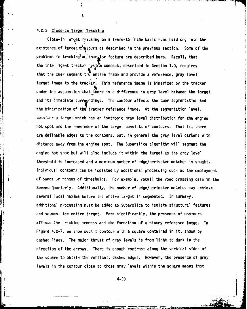
affects the tracking process and the formation of a binary reference image. In

Figure 4.2-7, we show such :• contour with a square contained in it, shown by

dashed lines. The major thrust of gray levels is from light to dark in the

direction of the arrows. There is enough contrast along the vertical sides of

the square to obtain the vertical, dashed edges. However, the presence of gray

levels in the contour close to those gray levels within the square means that

4-20 i

S, , IW, *' '' Z -'T T • • . i rl

)-

Figure 4.2-7. Track Square with Contour

the contrast across the vertical edges is low. In other words, the gray levels

in the reference target background will be close to those In the reference

target image (the square) and the track window may wander about the contour.

As in example, a 3x3 square just ahead of the hot engine signature was

chosen by eye; this square seemed fairly repeatable in series of images: 1784,

1788, 1792, 1796, 1800, 1804V 1808, 1812, 1816, 1820, 182 1828, 1832, 1836,

and 1840. These are taken from the set of imagei Jescribed in Section 4.2.1.A

The square was selected on images 1784, 1804, and 1824; this selection process

was a substitute for the cuer. The intervening four images 1788-1800, 1808-1820,

and 1828-1840 were tracked with the binary correiation tracker described in the

Third Quarterly Report. Tracking was attempted oo the raw gray levels and

gray levels processed with a 3x3 median filter. In both cases the results were

sporadic. The problem seemed to be that the square we had chosen was really

located in a contour of approximately the same gay levels as shown in Figure

4.2-7. The tracker, then could move about the contour with the accompanying

J 4I• change in shape of the reference as it was handeO from frame-to-frame. Thus

I by the fourth track frame, the aimpoint shape had changed substantially.

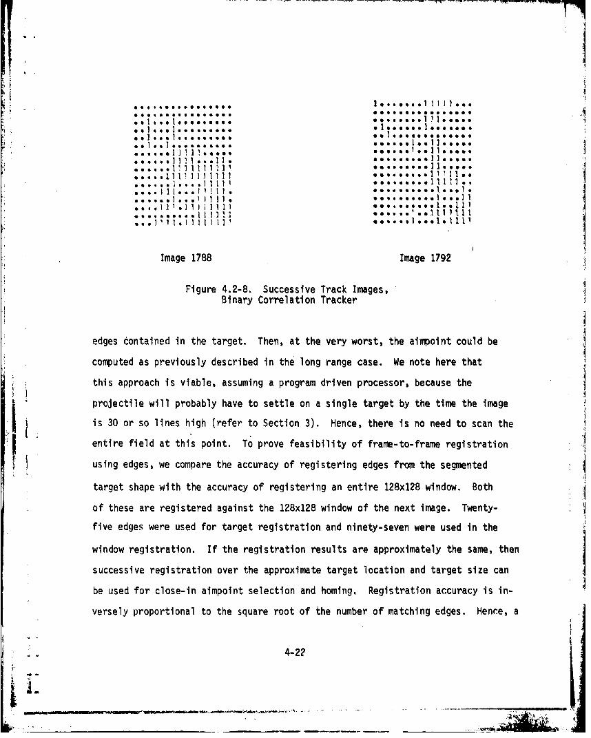
Figure 4.2-8 shows several successive track windows from the 3x3 median filtered

data.

Based on this data, we decided to track over the entire segmented target

as shown in the previous section using extended edges or subsets. This would

allow us to take advantage of the repeatability of a large number of extended

4-21

4 5 - V

~~0 a O 6 0 0 9II6 i 0 0 I a

00.Imag 1788 Imag 0.e000O1792..O,...90000*0000* *SO0,.0000]0OO00

0..,. 1000.01111 *o.o....,11]....,°.,0..1010000 *1 1......,o,1.L.....

00,,11 11] 111] *o,,,,l,,,1,110*

Image 1788 Image 1792

Figure 4.2-8. Successive Track Images,Binary Correlation Tracker

edges contained in the target. Then, at the very worst, the aimpoint could be

computed as previously described in the long range case. We note here that

this approach is viable, assuming a program driven processor, because the!I

projectile will probably have to settle on a single target by the time the image

is 30 or so lines high (refer to Section 3). Hence, there is no need to scan the

entire field at this point. To prove feasibility of frame-to-frame registration

using edges, we compare the accuracy of registering edges from the segmented

target shape with the accuracy of registering an entire 128x128 window. Both

of these are registered against the 128x128 window of the next image. Twenty-

five edges were used for target registration and ninety-seven were used in the

window registration. If the registration results are approximately the same, then

successive registration over the approximate target location and target size can

be used for close-in aimpoint selection and homing. Registration accuracy is in-

versely proportional to the square root of the number of matching edges. Hence, a

4-22

IVi

larger number of edges are found in the 128x128 window, and registration

between windows will b~e more accurate. This will be the standard for comparison.

However, at close range, the density of repeatable edges over the target

should be higher; hence, successive registrations should be fairly accurate also.

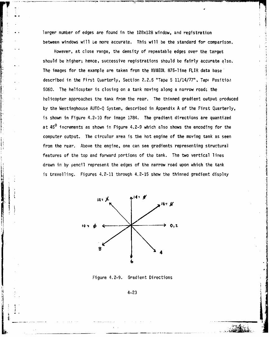
The images for the example are taken from the NV&EOL 875-line FUIR data base'

described in the First Quarterly, Section 2.2.5 "Tape 5 11/14/77", Tap( Positio.1

* 5060. The helicopter is closing on a tank moving along a narrow road; the

helicopter approaches the tank from the rear. The thinned gradient output produced

by the Westinghouse AUTO-Q System, described in Appendix A of the First Quarterly,

is shown in Figure 4.2-10 for image 1784. The gradient directions are quantized

at 450 increments as shown in Figure 4.2-9 which also shows the encoding for the

computer output. The circular area is the hot engine of the moving tank as seen

from the rear. Above the engine, one can see gradients representing structural

features of the top and forward portions of the tank. The two vertical lines

drawn in by pencil represent the edges of the narrow road upon which the tank

is travelling. Figures 4.2-11 th rough 4.2-15 show the thinned gradient display

SZ~ A. 147

4-23

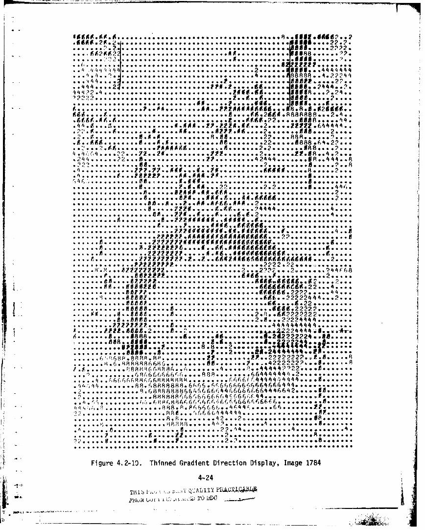
0J

AA2 .. 2 • . 1. .. ... . . A. .. . ..2 .001

oo... . .•.,.ooo22 o. *0000 .. ~ .... o..umuu *So,... 00

* .'V�. ... .. ooo':....... .. o...oI.. ...... oo ll .. . .

• • ... *.. .. *.............E1.. g. . .. ••I2Z~llt. • R ..2?...*. 4 008R810,•S 1*,2021.0.1... ,.2...... 1 . ...l.. .. 4

.. .14.. ,.2.. some. ,.2, om.2.... ..1 .o2114,.,

.'4 • A, . ...... Bo** * **. . .*...2... 1•€ € t . 221.. *.. 4!111hP. o.o 'I..

".191 Of. . . .. .... .... . ... ... .22.22 . ... ......

o. ... a.. a 9 o. 0 . RA -1 0aA...... ... 2. 2 *.... *8111 a.. 6 .....f.... ..... 4#I..PP2/I/I141{I•I••...1 .8 . .21..•,

e? o 0A o ..0 0 .o o .o....... A.,aoa,8 .o a0 &o*o ,2 2 o , eo .8 A .oe. :? o.

.. . ,s ..*.a... *tR,. 9 ,7 .. 0 2 .... . 1... 000..

00***. **.... 00.. OI...¢ SA.O... 2 ........ 2., 2 ..... o..°2.. , .

4 o . o..0. 0 4 *1o .... .2o, ... 8 ...... o2.. a

000,000000000.. ... 090..I• , . , o° ? 2% .. *• , °22 0.. ,..48,, .2 , °."•"00000000000. 0. A. * .279•/• .... .. / *.-.d ,-.2,2... .* .,o 88°,o .?0.,

o.*....o.~ *6666 0.0 .9.79#iM 009 * 0~0 00 00a0 * 000o0o00000

0 0 0. A0.. .2 o re 6414 g .0 e00 0 a 0 a0 0 0 a

0004000.00000o00000009 ..0 ? % 9 % E.o°, o°2,,. °..f.0 0 0 , .R,,• ..9

a o 4 * 9 *

*.g.o... .. 07222..... ,,,,.,0 0 a........ . . eo aS........ . .. 9.. ...0 00000 .a . ... . .. 2... . .. . . .. ...... ., . .. .. ..

..... .... of too.. w x...o.., f . ...... ...2 . ... .A4..

$ or 00.0 0 0 0 0 00 . ........ . .. ..00 .... f04,0 ..a ...9C.. ..9 A. 2 . ...

* 00 .%% ** 0~ .950 27-00 1~ P 4 e*# A0 .00 ON1999199 ,.. 9 . A ..

S..... ...... PI S o..° ...... o. .. ... 2..... we ;.0,..0.

* A..... ...... 0 0.R. . . . 0 .. O . 4 0 0 o 1 .1 v.&P .0 22.1A.. . ,.. ...P.

P0000 -99P1 ... .. .8 .6 j . ..... 9. .o0o os - ba*e * 22 22 ao . 49 . *. o

. ... . I , ....... 6 6............ .............. 66A .. 2. ... , ,€ 0....

.. . . .5 ... .... .2 .•i .. . .. . 1 ! ..ft~¢• tl l ... . . . . . .., . .... 1 69.2 2

* . .... .o a %. . . .1)P)CO.. ... 66 ., ........ . .2 .. . . ..

*0. 00000000 .P.......66..6A.. .... 66. 000 00.... 000..

22 ..oo...o.ooooo ... .... 6~*4 .000 ..00000002 000000.

14.2 ..... . 2 o .. .. o. . .P .. .o0 .*4@ 9 2 * 02 00 .01..0 220400000 o e. ..o ..

00.......... . 40000..... .8 .. ~8.... . . ... ...... .. o..I{{ .2222. ....... 0

........•..188. 19 . . .. It ... 2 .. •2 2222224a.eg .....

0400... 0 70000090002 .. ,.*.............@..***. .o•;;•) .... 00 •0 ••'" . ... ... .. oooo•-.U ----- 1 .o0., *e. Qooooooo4000 .o -(s - • • • "

4-24U. .. . .i.. . ira'.~ ,!.j.u..., .t.L .. 0,.•12 4 4 -, J• •. .

... . .. ý)8 ,6 .88 Tip SP . . . .o eaooo oe e. . . . .P . .22 22222?. 1. if . . . ... .. ... .6. R APR8, 6 689 . .. V,4 9*o11, . ... 4q,° 4°4222 222•- , ... o 8 91., ..... . o, 6 51t,6 66A 666f ... . 888 o , o , •~q( ° . . . ,•

4 . .. q .. 66-)G6FR8(,rG688RfSH e ao,. o,,,,, ,(, ••(•,6 r.44444: 4 4444 ,, o , %, e * goo o4 , :; o- & .. .. 8 8. ý' 888 888 8 *6F,()6S or • 6r36f66 6666 4666• 4£ 4 t4o * o • * ... o* * o'

2 ............ * *3(i. G 888888366e& 666rý44(j 666t,664446642° go o *I oe ° %1• 9

.•, •%° v o 9 9 1, ) , C, 8P f , 81(, B 66c6q6r-,!;66 (--666r,ý,6&6f!( a * 0 o ,, 0 0 v • 0 4 -Joe

2 2, . RA... ,9 °, .F•• . fj 666() 44 44 ... a, , *. 9 o° o o M ,,°oo,*o,. ~ ~ ~ ~ ~ ~ ~ ~ *29?* o, o o°;.,,,,,,•}H,•,et•°oo- o- o,-*o- °o@R'o0 o%°

S. .. .; . .. .. . .. .• .. . .. 0 . . ..... . , . .. . . .. .2 4oe o...* .. o .. ,.

Sa0 a 0o o0 00 0 40 00 °o °°0 o 0 o 9 04 0 00° 4o o o° o e e o oe 0e o0

,4 Figure 4.2-10. Thinned Gradient Direction Display, Image 1784

4-24

"q ' '.•i•T~i [,,z ,.., :..•.,7 'ALITI Mlka4.4(AW_

~~~~~~~~~~~~~~~~~ ru ,,I••)DO,'•-.. ........ .. ... .' .. .•

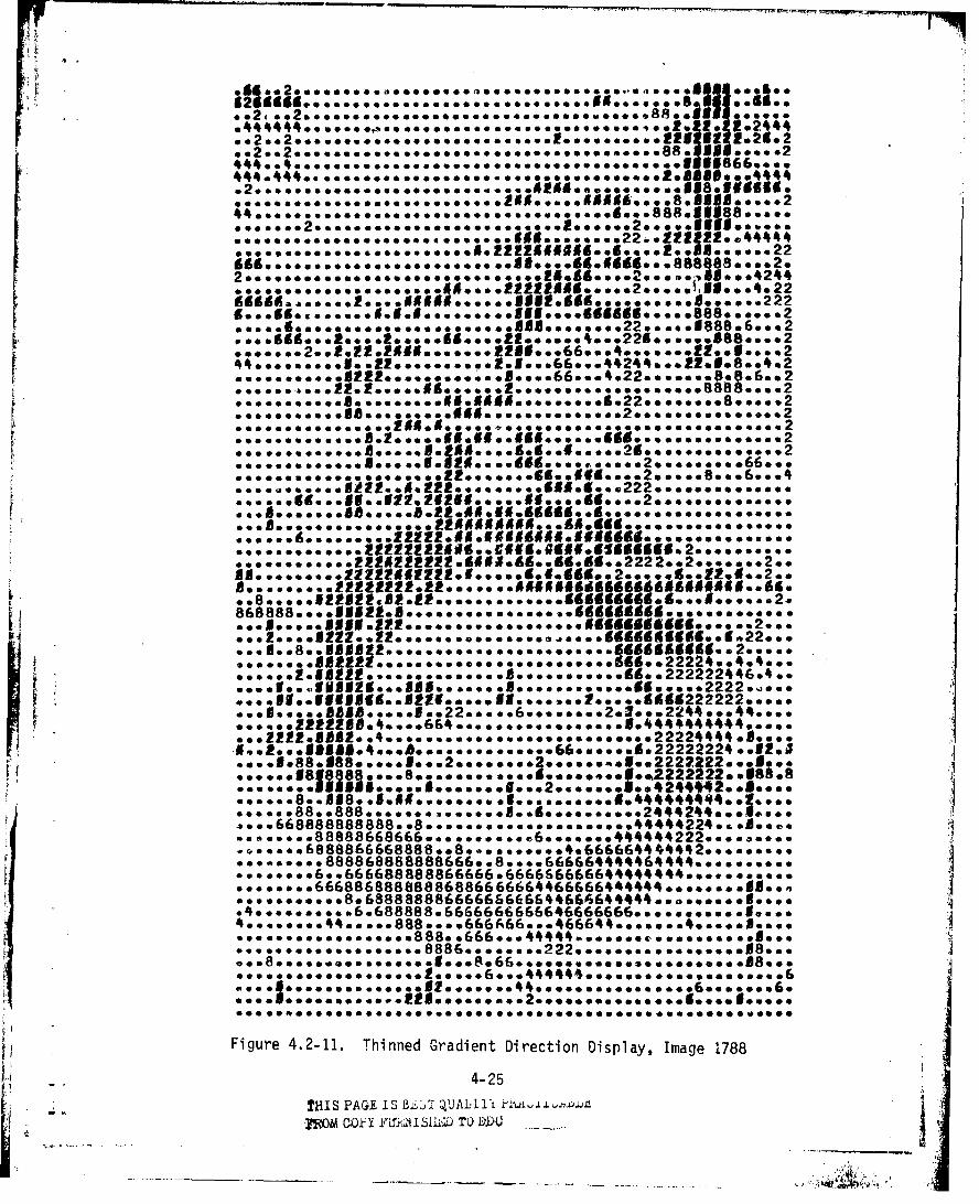
- "I

600000000 *0009000.00.0*. .. l.oooo2 .2 919212 29

002002*00600 .eseeooeo soooooooeo o.* .o~oeou 88 .02244666066660:6000000:06090,08S... so...... 06000 388 668.0 s2

.............. oooo~ooeo~o. oe .4245.. @50006000198 g* E1 44600000000 000 00000060100006 faa..... o 2445 * 1.8 *9188 o.22

2 6 o,.60...060ogof.0.0.00.02105500002000.,890004o24

*..'.000s800ooo..22.14:.'1o""'.'.o..oeoo.oe..:: o~oo*000 50a: ooo50.22.ooos i.igiaagaaa *ii1941122oo. 000086 00o

Am. .. *0. . .l22222t6So ..V .. go *w*~1.911..2... *oo* .1.000002.

:.8.Z. ooo a ogo g oo29191.499044* a *11C11sid 1..o, *eo* oooe2

00000 **00*0~t~**~ 0

06O0060.2.821106 ............ 1.22224.

0 It* .6U69891. * DUe..... e. .. . .. 2. .. ..11222222... 0o

000 .. 2229A.4....664... * .............1.4444444444.....::::of 0 99181......ssOooo..s....66o-oo.5ooS22ig222224 ,2.*

......8.ag.18..4E........ .l.....ooe..oe.444444444o.Eo...

....688888888. .8..... ...o...e .....44444222249.. .8..

~o.o.6e888866888 88..8.o..oeof......4.666664444244o....o.o. "0o0 .. 888868888o88666. .8.. *o .66666444644424. .0 *. I

::::o... 88.6688868866666oeo..e6666666644444424..... 00600

0* .. ... 666886888888868866 66664466666444444 .. ... . .81.*6eg soooe* .. 8.68888888666666666644666644444 a*oeoooge.0bo s.4*. .... a. 6 688888. 6666666666646666666.. 0 oo*0***o

Figure 4.2-11. Thinned Gradient Direction Display, Image 1788

4-25

THIS PAGiE IS BLJI QUALI'IY i?'.

d rWM GO.FY YLi~ll ISL TO D.DU __

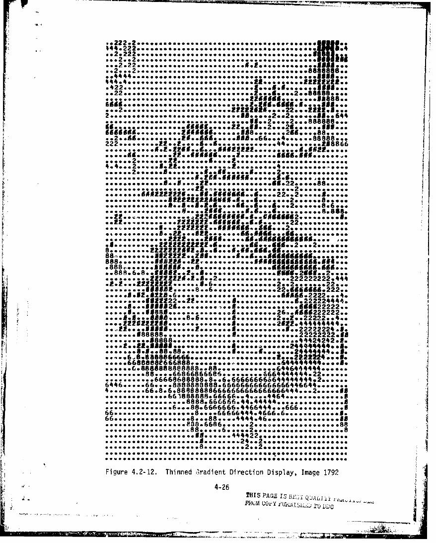
age

61651161 ................ t.E.... 1118... :!189 oed: deo 06

00 000000o0oo*.**fgnooooo****oo 99. eo*2..2.. 888888..

* 90o:..O80000 1.oEIgj .....081 ... 2.........

....... A~ftflU..ft.19U6..6...2.......8.....

.8.o*-0........fo*O**oeoooo***2222t26...6. 6.2..22.......

8~~..... .... 119960466 1422222 tI~.i.aE.6.5.... .o.

vlo9..g.98888 ooe. .. e.oo... .5 o.. .. .. 26moAU666222222**

.... 88...8*h...8.S.o.. e e..,..... *.t.22222224.1.. 2t....988g888.....2.......g...........g..22222222*g.

gee. 2 8 8ooeoooooooooooooo~ooosoo~e.vao4424242o8.

e ....6B8ae6§66866686..... oo....0...I..e2422o~~ee..I

g..........66668688888.8eo6.66666666564~444~44442......64*6....66e...888888B8888.666666666666666446644.......

0S0000000000000000000*000ooo886000046644o660000000000o

Figure 4.2-12. Thinned Gradient Direction Display, Image 17921

4-26T~HIS PAGER 13 BiLf UL1

. 7M 1Oiry -. ýw

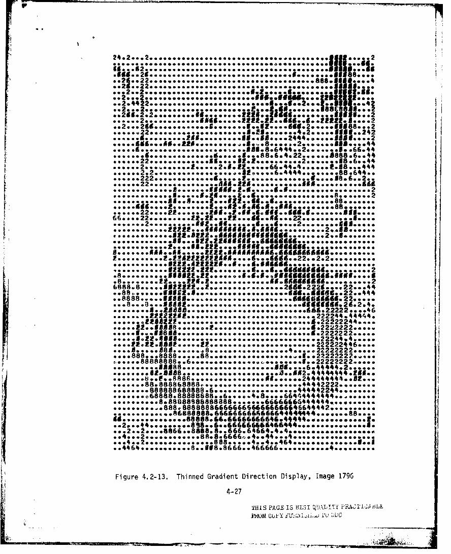
- "V - - -es;

99

III

90 00000600 4,o0e*4

.022.......~~:: ::: 11 1:::2.. 0 0 6. . . 0 00 0 8 9 . .

oe~o22ooog.......::**.s.2%2e.....aao.. 2t2t*.ee.o 221... 2

9*.....222o.o.e.o.2...too.. *t2oe***e.o~o*9*6.*9oooo

92*2422221. 1.. 9. 9595.. .. .*... ... .*e*4

,.........2122.I2............95g91g9.......2o:

6,oo888.8.....S9*2*22..200....... **....2959.2229..222...44

:.: ..s .. S ........ .... ........ 1999.22ft

*o***s*88o888.8882...2............... .o44222222446...

*....8888o86888868.6........eoeo........44442444*. 0.0.0.

......... 888v888888BE666666E4666656665I46644442.........

Figure 4.2-13. Thinned Gradient Direction Display, Image 179G

4-27

i'lI S PAGLE 15 BES T QIJAL T YPA- ?i A ,4 1jhl

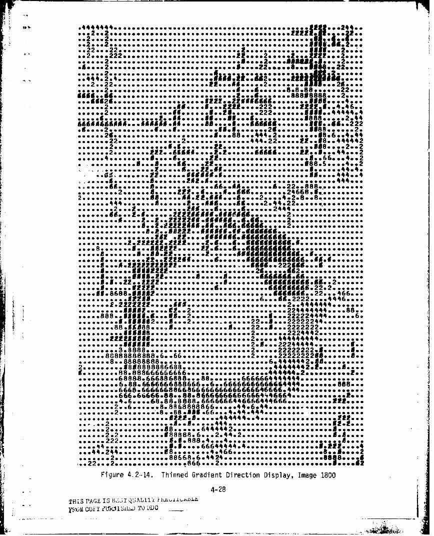
.. s 2s ..

Ir

.... 2 ................. eSoees .22....................388.e....4.,~~~~~~~~~~~~ 8..a..2 e.oat.Esas.a.ae55aeaa. 4 42~

.e24e8eE'e'stei goes*

000000*0022 .... 2....C5444........

.....d........12t..........5...52aeaasas

esas~sa a .. 68888.666ooooo88688822...ee2222eeeaoseeeeo

SN.2. w6 8 . ......... scea~~~oo2444ooomse seas

e*4aseas.82886666666BRaBB 86 Ss...aoe 4 .Saooosoa4asa..aos~sa s.a

.... 2 2.e 2sc.e........... 8 & . 2 .a.s.eee....

Figure 4. 2-~14. Thinned Gradient Direction Display, Image 1800

4-28

THIS PAG.E IS 15 ULFffvUM Gui jja 1 TO WU ~cI: __ ____ ___ ____ ___ ____ ___

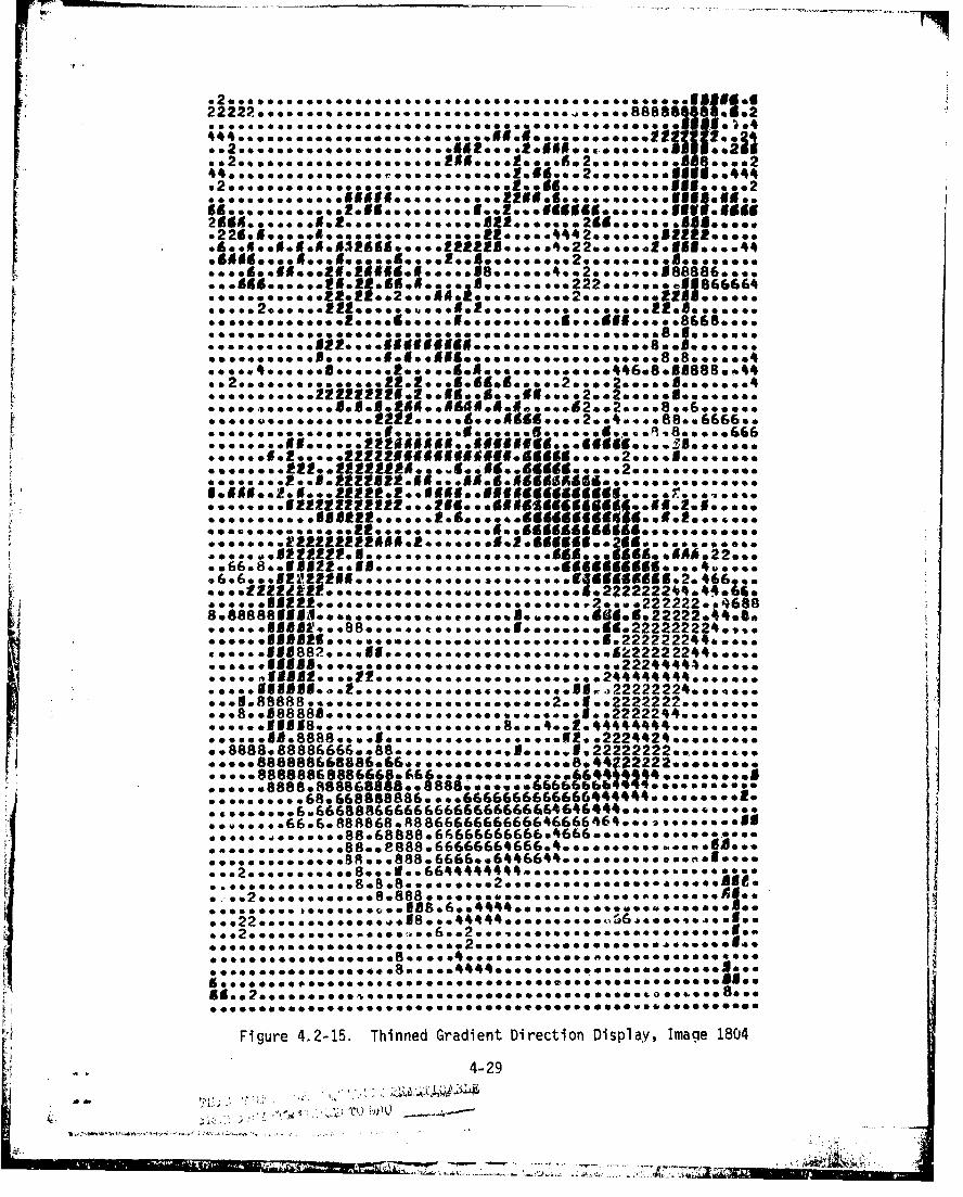
* e0g.... eae** 2ss...... Bill '4.. e.. 91*M

... e.......2...e~...... ON .2..c..Et1.....

*a* so *so *99212 2 116 of* oldo *So **Of*** o ... tte 0c..cee666*040060000feceeecsee .e0e.e.ceSi~.e

.e.......009000009 e.t.eEE N E S c.eP%...c.8ooE.....

...... 222. 22 2 2* 4 .cw~.Ei.EMCC~~e2..2222244..e0

**.....*1'2222122415*.......E.2.6S66i6..99266............

*eeej9 2 2 !*.I.......e.........eelE..eSM*e.UA.22..

.... .188*888...88...... 0000 #v....E.....2222222224o.,.:

......d8.8eo88*888....9...6e. 666ec.e....It. 2 22 4 o2 eeese

.....888.8S8688i................ .....b&,q.... .e...0

Fiue421. TindGain ieto ipaIae10

... e~e.8.888c6666~66e.eeeee4-29elee

~0 * .. *~ Ce. .e.. w

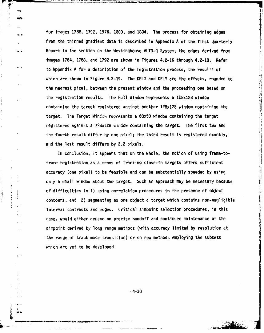
for images 1788, 1792, 1976, 1800, and 1804. The process for obtaining edges

from the thinned gradient data is described in Appendix A of the first Quarterly

Report in the section on the Westinghouse AUTO-Q System; the edges derived from

images 1784, 1788, and 1792 are shown in Figures 4.2-16 through 4.2-18. Refer

to Appendix A for a description of the registration process, the resulfs of

which are shown in Figure 4.2-19. The DELX and DELY are the offsets, rounded to

the nearest pixel, between the present window and the proceeding one based on

the registration results. The Full Window represents a 128x128 window

containing the target registered against another 128x128 window containing the

target. The Target WInd-,,, repcesents a 60x50 window containing the target

registered against a 1?8x128 vrindow containing the target. The first two and

the fourth result differ by one pixel; the third result is registered exactly,

and the last result differs by 2.2 pixels.

In conclusion, it appears that on the whole, the notion of using frame-to-

frame registration as a means of tracking close-in targets offers sufficient

accuracy (one pixel) to be feasible and can be substantially speeded by using

only a small window about the target. Such an approach may be necessary because

of difficulties in 1) using correlation procedures in the presence of object

contours, and 2) segmenting as one object a target which contains non-negligible

interval contrasts and edges. Critical aimpoint selection procedures, in this

case, would either depend on precise handoff and continued maintenance of the

aimpoint derived by long range methods (with accuracy limited by resolution at

the range of track mode transition) or on new methods employing the subsets

which arc yet to be developed.

4-30

L,,d,

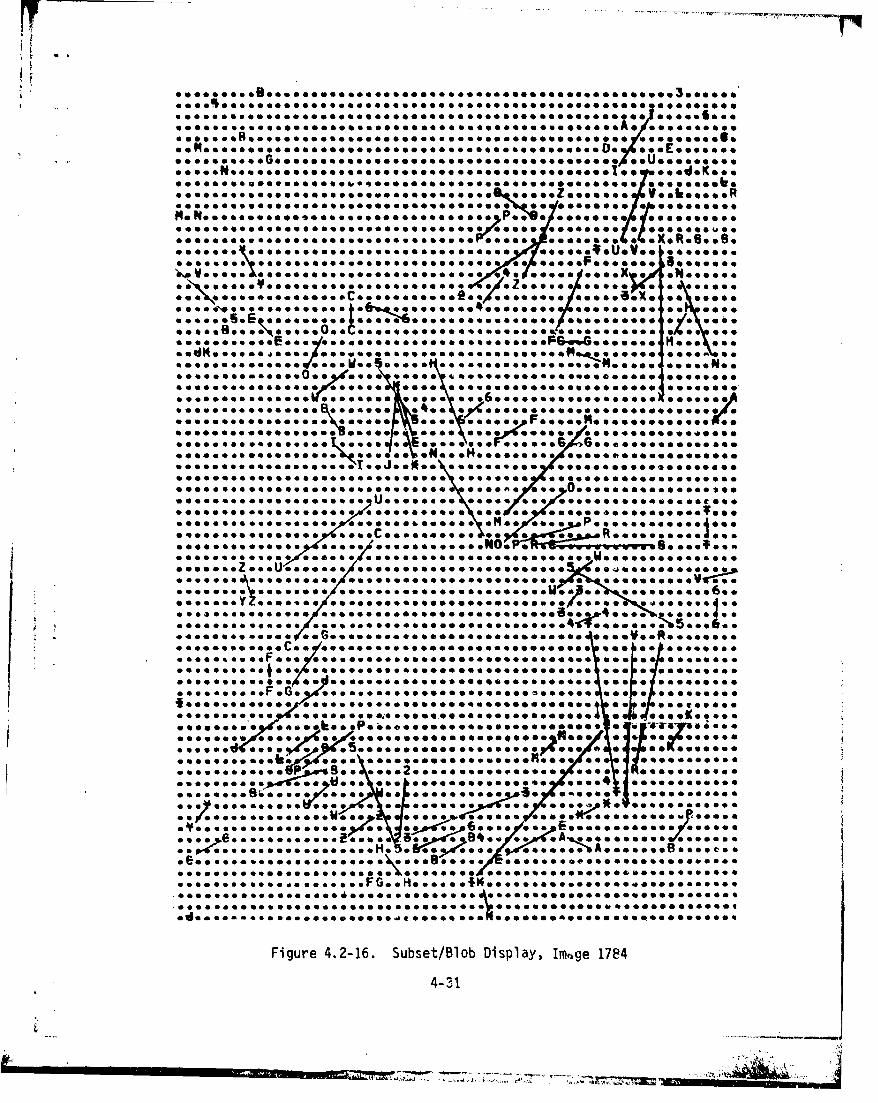
e.9..eeeee... eeeeee....eeeeee~o oseCdoeeee

04*eeeee *eoeeoe eeeebee~eeee.eeee*O00000 :qoeeee oee ee k~o

0 e0e0eee C~ ****ee s~i.esege. ~eeeeee.e~eee~ee..e~ee. . e oee ou:ve a**:::::

...... a.... :...eooeoe~e~e 00000000e *603x eci.G::

.....8..0.0\00000004 0000*04,eeehe .ece.eeeeg .ke . e...cN

e.~~We..e~eee.. A Rangeeeeeeeeeeee~q e *c *0 0 *e. me

***@*e***** ~'eeeUe ~ee~eIeeceeeeeee.. ee~eeee*. 0.N.

x, a -a a : : : I- : : : : c -e. : :: ;: : : :: :: :: : :. 1:.e.. : ... ,.ew

eceeceeee..eec..~-' P4ce. 0400 0<eeeee 0eeececc00e00

eeee~~~eeeceC~~eeeo-ee omoe.1 ec e.oscc.. eooeee: ac:

"a A6691400e..69 a~.tce~ecee

eeee~eeeece~eeecee~eeecCeC esceece eeecc0ee0eecceee0eececeeeeeeeeeeeee..ec~eeec 0set 0C eeeeee~ee

ece~e~ee~eeeeee.ago U.ec0eee 0 e .eeeeeeeccee*e~oee

ee..ee~ee0c00e ceeeeoocc see* aMe *..e Roo**ee~e~

e:: ::: :::::e eeeeeeeV

00004 009e0e.ce. . . ,ec .. ee.c eee ce ce. .. e ***::s e0e0c..e..ee00 ce6c04000 000eeee00eee~e.e.. ee~e eeee

eee001eeCeeCegecee goc Oleeecc000,100600*00000~ecee *0 * C~CSCC

Icee~~ce~~ee~ ga ceeeeceecec'coeee. e4 e...eeece~~~~~~cec~~~~~e .. e -ece-ee.eeeeecee b cea..

000e0000000c,.* e.ee0e.eceeeec~e 0* 0. p 0T0ec... e~~~~c~~~e.0 ee.. .V4eeceoee0eeece if

eeoc *~ ~ee. ee~c. .ceec~e. * :a 'o.1 *. eceece

awe*. 0 cc::;V 0*9V~..w4~ 4, aeY a 'eeceeccec 1

c4m e.e0e.ee..He~ eeeg.0: ::: A:s 00*0000e0*eceA

c~ee~..e..e..*eeeee .. S e0e eC;~,eCe* 6000000000

.ce~eeeeecceeeemee eeeeee eeeceeeueeceeeeee00c

600000::: ..........

Figure 4.2-16. Subset/Blob Display, Imqge 1784

4-31

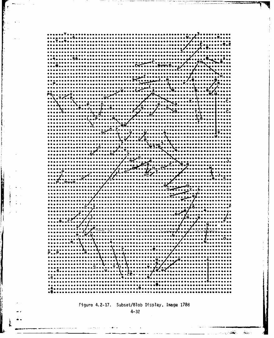
.ee~~~~~ee~~~~ee.~~~ -7g eeee...* ge b*6SggO*OOC *'***e-

gegoegge~~~~~~~~~ aeee~cce.geeegce*~*cg so *C..c..**A**

*eeeeeg~eceeeecg.eCOgccge e w"eeegc**acecccg

.... 4b

*cgcece~ceecgcgeeeeg.eee~g~gggecggoso d eo... ooooo eec.

.:: 4 eec..

so* gee..000

000*000eeoc.

eec. gee.

ýOls&*:N o*O6OOOOS**IO* Cg

*g4geogeecegeeoe ~.00000 eecgeeeeeeeeeee.e ~~

.*eeeeecec~eeeeeee~ee so***Jeeece 3..eo..e0oe0e..e00...e

e0 00g .0 e e e e g c . . . e . * . e e e , 0g j

e... c.. e... ... .... eee ee~ee~e~ce 3.e ee. ee06060*0006009*ee~eeee~ee~eee~ee~e) .......'3. ee\c..ccc0 cceeeee

O*eg Peoeo*egg .4'.... L4.ec.e ce .0e4.........e~ec.eee.ceeeeeeA HT.........eeeceeeeec

.ceeeececee~egegg '0. ec... ec *ec ccc.e..

Rlrveceege.oseee.oos g c e..w ~~cg .geg~e..Jgeeeg~geeece~egccec ~geeqw89....e. Ec. 8...........

eee..e~ee..~eeec~e~ce. . .ee.e .e..eX

.c***e e*eo * ***.* o eegeeceeosgee 00 c jeeso ofo .eeeece...

.,**e***0e 0 00 000,000000 0000 0000000 T-9-460006066~e~*~oaes"eee*:e 0eee.eec.oee0cgce. 90e066ecece...

****** ...*Roo** eeeeeeeeeuceceeY.f.ee.ee

*.egeceee..eee~o~ 00.ceeggeeegegagg*e.e*c.e~

e*.OgeO oe ossge~ .e o.e~oT .1. Oeeeeeee oooooOSOOC*oeceeIs. ee--eveeeeeeeee.eeee.

R. ~ ..e~~~~~ eeeeeegege.goee.*eeg c.ece~e.eceeeeee cc soe~cegeceeeeecac~e ~~egc.

-Aw A

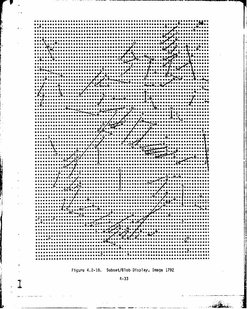
-77W+ * .... .. . ..... . .. .. . ..... .. ..... . ... . . ....c.. . .. s.......... *cc......e ............... ,eee eec e ~~ e OO ae

O~~~~~~~o~* 0OO O O O O O O 0 0 OO000 *0000O0O0QO OQ

.ecc.cO..*cO..e 0*.@eOOO~oeOO*OooeeOO Ooo~

ooqE~ooo oes~o

*o. oe ooo~e ~ ee c eeeeoo oeeo eoo oc oee oe oooee oooceeoooo .#o.oooo . ooo

*.*. *.. .. ................ ,.... oC O o....., u..... .... ee;;•' . . . e.e....e.... ... e...eo.e. e....... ........ .... ,,, e... ... . ..ee. . .,e. . .

** 608066000466

... o. .... e.. ... o ... .. c. .... .... ,,, e.e... .o c. .... X. o o. e....

c.. e... eo.... .. . .. . ..0 c...

, .e..0.0. e..... .. *.... ... . O.., o...oe oEo. .,e.c..e c. .. c.. c.qc 0 *..0.

.. e u.@ ................... s.,...C .ee.je...... c....... I.. ee•..e.c.. ...

.. ee.ce.e......c......ee.e.........ee... .. e.o.ee.e.....\...o.......... ec.. ce. .. eco.........cc..... ... ~.. .... . . . . . . . . . . . . . t

so. ....... . e. . ~.eceeeeeece.e,.e..e...e..,.....c,jeVe~e e.........R........................e.,e.e.o. .. eo ~ece~eeeee A.+e 1e ee~o~ e oooqoo.o e..eo ee ceo eecoe•.eoe.. ce.. .. e.... ... ... .o..c/..o .. . c..... ,.. e...... .. e.. e.e.. .....

.. •....ooec.e.......,.c....j..•- - - - - * - - - - .oooooo .o..ee. e......

... o .e .. . e. 4- .. s. .o . d.... . u ,e-, e e e e e.. e e.o o -tj. o ..:: : s o.o . ,o .e.e......c.......H .e...•. .e.....e..,cccee...U. ee......eet..,..e...,• e.....e..,.....c.....,...c......• e.,o.e......., ... ec..d..........c......c..eHooc o...o........,c-.-@c*..--co•---e--..-o-T-o..-.----

. . . . . .e.. . ...... a . ../ ... .• .. e. .o. .see

.............. fee........e..oeq.....,...c.........cceeccce....c..!.

• .. ..+. .... ........ ee. ec... .o .. c. • • . . . . ....cc c ce O .~e .ec.. e.. e ...... c.e.............ee..e.... .... T..Ucce...vc...ce.....-.-....e

.. . . . .. . . . e. c.... e.. ...... ...... eee 'ee -eeeej. .e.c ~ .o.eeo. .............. .•...... •.eceeeeec.............c.......e ..... cc.....c.......... ,.ecoe. ce . c, .e... .c . . ..ee •. . .....ee e~c e c c • . .....e ,•- e . ...- ee.c..e..e.......e.e........o............................ ccc.........OcOeOceeeO.eO.ccO•.e.eee....eec.OO.OOOOOOOesOO.c .OOOOO0eOeOOOOO..c

___ cc:~:: 0 0e 04A:.:..0oooeeeo.,c. o(cooc.o.oop. 6 e.o.,cccoooo.-ooceee .oeee.oe. -o..ooooeco....c... o~o.o.G•.oeoeo~ooeocoocooo-..--..ec--oV. c.-e.e.-.o-.A..-e.. e... ..J .... c. ee.e oo.. .-.--. .ee ..--.--- Oe----. e--- -----------

........ .... ................

c........c.......c....................c.......e..c.... ....... cc...eooc eecco eoo eeeoceccV c eooeoooo eoo o ceooeo eeoooectecchieoc oeeece

cso.eeceeeeo ~eo.•eecoo ce c ceeecceceoocoooooo e"eoo ooeeoee~cce ooee

.. . . .....e e e .. ..cc sc.... • .. c... • .. ce.... e.. o....e.. .... ... ..

.. .. . .. o. . ....... .. . ¥ . n o. .. .. .6.0... ... .. .0

• , ... ... , . .. ... ,.. .o. ].,•+ .•.j.. . ..... . . ,. , . . . ,... cec.oP .... o....,,..oS ... .. c... ... c.......o.... c. e... cU . ..

Figure 4.2-18. Subset/Blob Display, Image 1792

4-33

I ' _ _ _ _ _ _ _ _IO •O • O0 1 OI I tl I II ~ lI • •O I tl O_________0_0___0___O____O__O_______O_____O____________OOOOOOO~

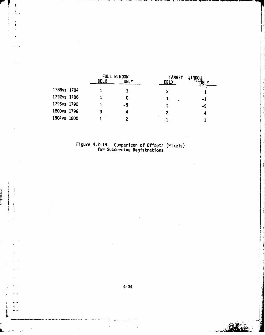
FULL WINDOW TARGET I.JIq ,DELX DELY DELX %

1788vs 1784 1 1 2 11792vs 1788 1 0 1 -11796vs 1792 1 -5 1 -51800vs 1796 3 4 2 41804vs 1800 1 2 -1 1

Figure 4.2-19. Comparison of Offsets (Pixels)for Succeeding Registrations

4-3

4.2.3 Tracking During Trans'ition

The purpose of this section Is to discuss tracking during the transition

from long range aimpoint selection and homing to close-in aimpoint selection

and homing. In Section 4.1, we presented a concept and examples of long range

aimpoint selection; in Section 4.2.2, we presented a concept for close-in 7

i!asegmentation and an example. c eto e, we consider the transition from one to the

other or "hand-over", if you will. There are two parts to the problem. One

question is the accuracy of handing over from binary correlation tracking to edge

tracking, another question is the accuracy of edge tracking itself. In general,

edge tracking accuracy, which is really successive, frame-to-frame registration,

is proportional to the initial offset between frames and inversely proportional

to the square root of the number of edges used. To test edge tracking accuracy the

following pro~edure is employed.

The Westinghouse lab equipment, at present, extracts a 128x128 pixel window

from a video tape. Thus, the largest window for the successive registration

test is 128x128 pixels. Within the 128x128 pixel window is the 30x30 pixel

target. Since the registration accuracy is inversely proportional to the number of

edges used, successive registrations of 128x128 windows can be more accurate

than a 30x30 window registered against the following 128x128 window. In other

words, the accuracy of registering the 30x30 target against the following

128x128 window can be evaluated by comparing it with the registration of the

full 128x128 window, containing the 30x30 target, against the following 128x128

window. Since the same window pairs are used for each registration, the offset

is the same for both registrationS. The data for this example is from the NV&EOL

875 FLIR data set as described in the First Quarterly in Section 2.2.5. The

video tape is "Tape #5 11/14/77", Tane Position 5280. It is a side view of a

tank, moving from right to left across the field of view. To verify the

4-35

JI'a " I : !;:S ,

,•, >' -

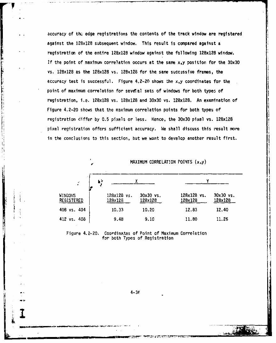
accuracy of the edge registrations the contents of the track window are registered

against the 128x128 subsequent window. This result is compared against a

registration of the entire 128x128 window against the following 128x128 window.

If the point of maximum correlation occurs at the same x,y position for the 30x30

vs. 128x128 as the 128x128 vs. 128x128 for the same successive frames, the

accuracy test is successful. Figure 4.2-20 shows the x,y coordinates for the

point of maximum correlation for sevd.al sets of windows for both types of

registration, i.e. 128x128 vs. 128x128 and 30x30 vs. 128x128. An examination of

Figure 4.2-20 shows that the maximum correlation points for both types of

registration differ by 0.5 pixels or less. Hence, the 30x30 pixel vs. 128x128

pixel registration offers sufficient accuracy. We shall discuss this result more

in the conclusions to this section, but we want to develop another result first.

MAXIMUM CORRELATION POINTS (x,y)

R 2

WINDOWS 128x128 vs. 30x30 vs. 128x128 vs. 30x30 vs.S•.REGISTERED 128x120^ 1284128 1284128 128x128

* 408 vs. 404 10.33 10.20 12.83 12.40

412 vs. 408 9.48 9.10 11.80 11.26

Figure 4.2-20. Coordinates of Point of Maximum Correlationfor both Types of Registration

4-3F

I&

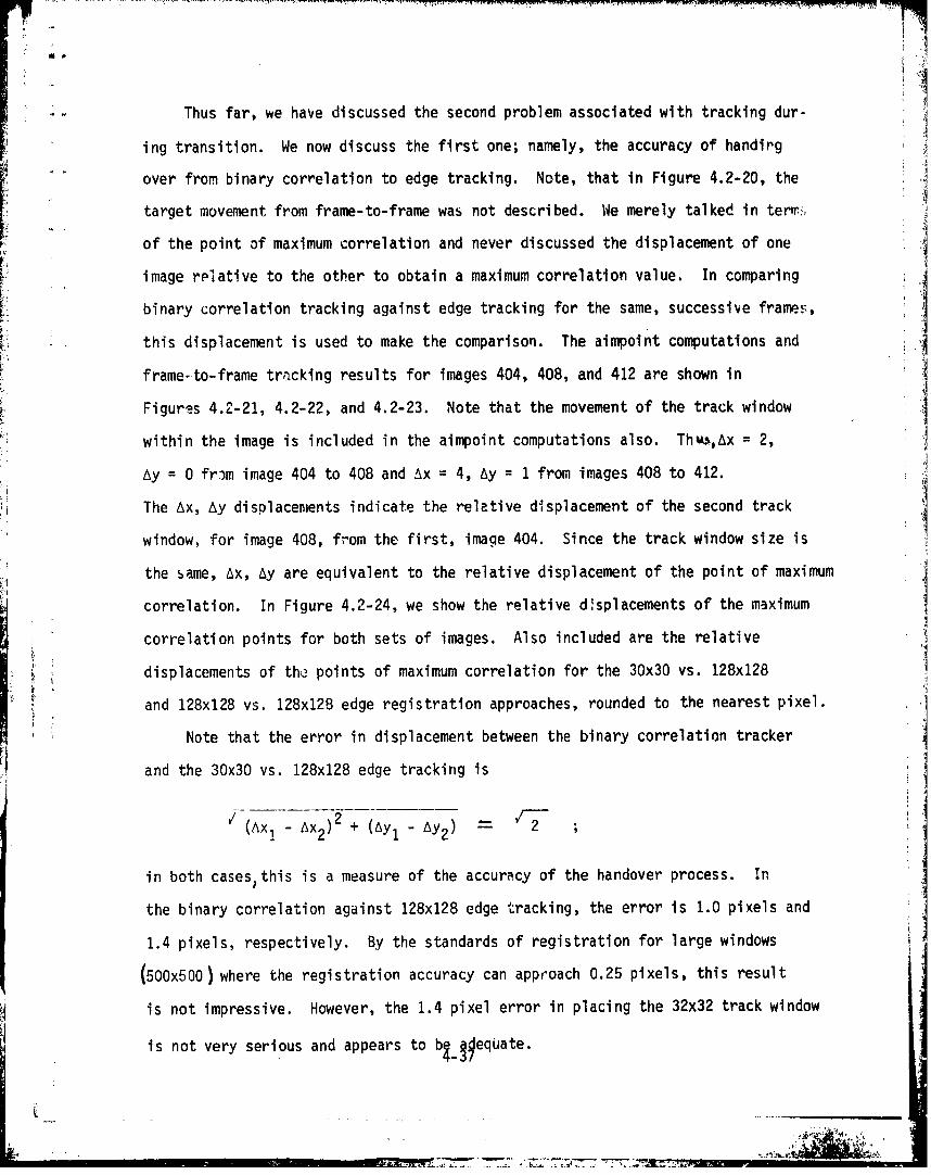
Thus far, we have discussed the second problem associated with tracking dur-

ing transition. We now discuss the first one; namely, the accuracy of handirg

over from binary correlation to edge tracking. Note, that in Figure 4.2-20, the

target movement from frame-to-frame was not described. We merely talked in terw..s

of the point of maximum correlation and never discussed the displacement of one

image rplative to the other to obtain a maximum correlation value. In comparing

binary correlation tracking against edge tracking for the same, successive frames,

this displacement is used to make the comparison. The aimpoint computations and

frame-to-frame tracking results for images 404, 408, and 412 are shown in

Figures 4.2-21, 4.2-22, and 4.2-23. Note that the movement of the track window

within the image is included in the aimpoint computations also. Thus.,Ax = 2,A

Ay = 0 from image 404 to 408 and Ax =4, Ay = 1 from images 408 to 412.

The Ax, Ay displacements indicate the relative displacement of the second track

window, for image 408, from the first, image 404. Since the track window size is

the same, Ax, Ay are equivalent to the relative displacement of the point of maximum

correlation. In Figure 4.2-24, we show the relative dlsplacements of the maximum

correlation points for both sets of images. Also included are the relative

displacements of the points of maximum correlation for the 30x30 vs. 128x128

and 128x128 vs. 128x128 edge registration approaches, rounded to the nearest pixel.

Note that the error in displacement between the binary correlation tracker

and the 30x30 vs. 128x128 edge tracking is

/ 2(Axl -Ax 2 ) + (Ay-Ay2 )

in both casesthis is a measure of the accuracy of the handover process. In

the binary correlation against 128x128 edge tracking, the error is 1.0 pixels and

1.4 pixels, respectively. By the standards of registration for large windows

(500x500) where the registration accuracy can approach 0.25 pixels, this result

is not impressive. However, the 1.4 pixel error in placing the 32x32 track window

is not very serious and appears to bj. 9 eqUate.

W

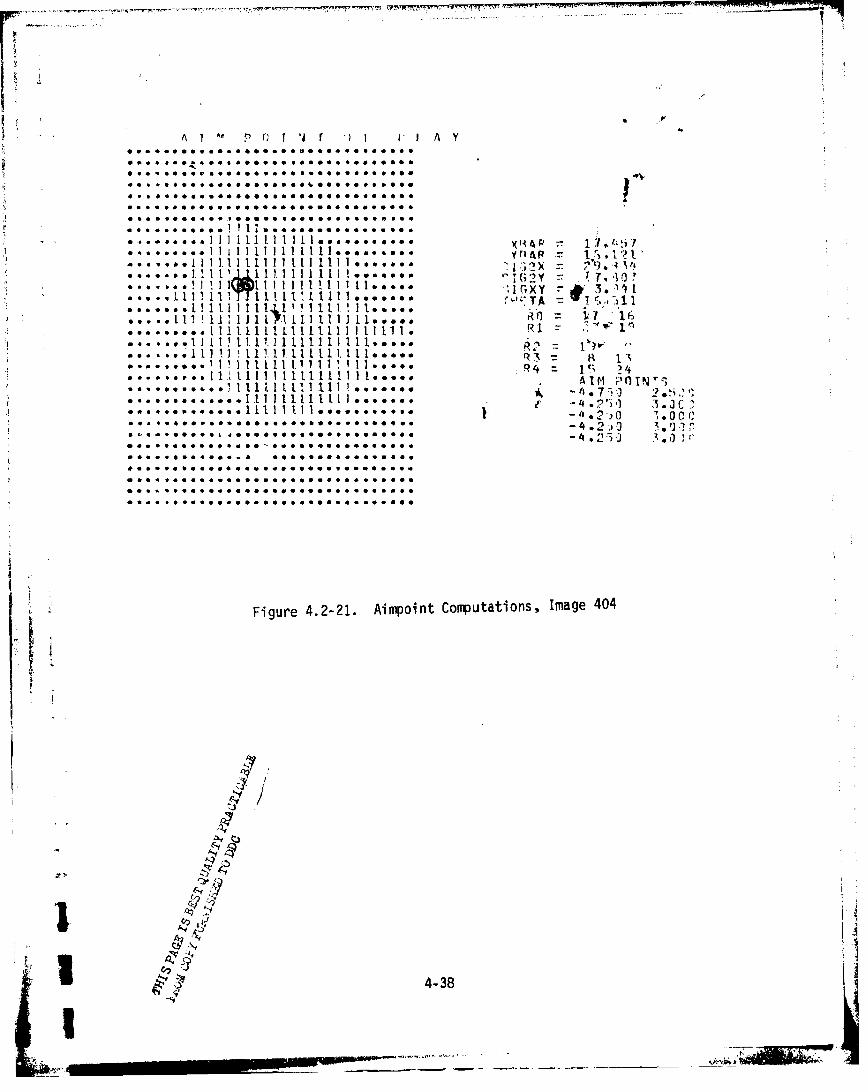
t' A ': ~ 14 iI A Y

*g**** e0g * 0e* @ eg 0 00 00 .. gg 00

0 a00 000 *e........e.&.&eaO.*eo..S

*gg9O@.gOO@Op O** ag90 a 0 ga

I~~~~~I 4*S~ P* *O *8O*O* I***

* eg ... 0 oIeY3 1 1 . .. e ... .

11 1 1 11 AL 1' 1. 11 1.1. J10 0a0

.... 1i 111 L11 i 11111 11 11.11 * I

I c c 1 1.1 1. 11 11 11 1 1 11 1 .. g0

1gO O g 00 1g 1 1.1 1 1. 1 I I L I~ I 0 t I0 I )o~ ~ aCeel oe~. e~eg~g~eeg~ gOCO~g 42 J ~~)4

e ,4~ee0.I eeeoogeegge~e.eo ~ 1r

0 0. *00 gege eg. ogoggee. e g..

000 *ooeegae0e.-4e2.C5 egei

Figure 4.2-21. Aimpoirit Comp~utationls, Image 404

UA

4-38

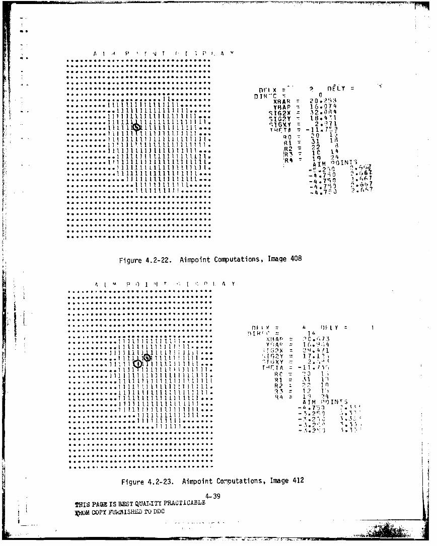
A ., P I r ,q T rP ; P . A

o 04 0a 609 a a 9 0 9 • • a q06 o L 6

0546.69600950 1.0 * 0 000700 04

9066~~~~ G2) 902 *. 040 R090 0 604

* 969 o•0o *•000 sOos.ooooeo 6* •o0600••

IO I60. 6 6 0 0 0 0 0 I096~ 1l~ 1( 1- 1n 1111 1106" XRAR T 0- 1 1 .

•.• ..... ~ ~~.... l 11 11111 1]i Ili • 0 . ..6Y69696. 7'

•.'!, . - •.....oo•. •llafl lllIIIll[I..••...GX : 20

R 51 I3

11 11.1 • .... 111II .II 1. t t LdIN1i 1 1.1 .1 11. 1 1 1 1

00009.09.0997 0004

e:.. . . . . I Ii t I I I I 1 1 1 1 t.l I.7E.2%

•.•-q4 7 6- 7-

iFigure 4.2-22. Aimpoint Computations, Image 408

"• ~ ~ ~ ~ ~ ~ ~ ~~n I y! 0ý I y I tJf0 iQ•lI~eO° 0tl

9.o 0066*6.6• 0060000090ooooe06 ooo

00006e o0 o60.0 66A Ae r, :6 o o 6 6

100 90 0 0 60 A09 16 6006 6 690 4

00 ?46 009 406 460 0 0 0 0 6 0

00 ~ 4 060 10 666 09 0 6 6 0 0 0 6 2

I 1 I I I II • C

9 6 0 000 9660090009406600166960

go 6 0. 9 .- 0 6 70 0Y .0

99 9 0 0 9 6 00090 00 0 6206 6

0006 0 06 s 9 00 00

..... ~ ~ .'*.'.'.'.•.'. . .. . .. ' ." .••F ..' ..

..... 60 609. 1 111111111T 1111 -12111.6...00.. ... .I I111111 1111112.16o0 Yq4 1 ('. 3;

606 909 49.1... ll l l lt ii111 Col A-IM.Tns I-a 1 .2"

THIS .... .... I I I B QUALITY..II . RI"O1 :

60........ .. !I1 Coplll0ll9t•.0 0l 0' 3r s.',C

0..... ..... o0 l0'0l60l0060096062 :66060

600.... ..0946 l6l006066950690063 6120l6•9 o ... ... .111 1111 11[I 11[I • 66: 16:.069 .... 0 .. 06I 9 I ll60 l 1[0lfill • AI 000,6"90o6.. ..0 ..0006000606960606606060.760 2.•

6. 9. 6. 6 .. .. 6 . .lllL06ll l0t 6. -. ,.6 ,".0

S.. .. .. . Figure 1.1 11.4.2.23•A-."oin.CoJ tat...,Imag 41

S.. . ..• .. .o .. 11 Ll ..... • - .°",-.4.-39•

THIS AG1~ S BES Q~t-I.,TPRAC'C-.LS.... . U...I...... .C .. .D . .. .. .".'C1. 7

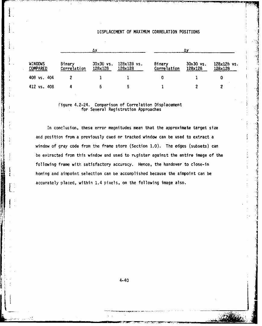
DISPLACEMENT OF MAXIMUM CORRELATION POSITIONS

Ax AY

WINDOWS Binary 30x30 vs. 128x128 vs. Binary 30x30 vs. 128x128 vs.COMPARED Correlation 128x128 128x128 Correlation 128x128 128x128

408 vs. 404 2 1 1 0 1 0

412 vs. 408 4 5 5 1 2 2

Figure 4.2-24. Comparison of Correlation Displacementfor Several Registration Approaches

In conclusion, these error magnitudes mean that the approximate target size iarnd position from a previously cued or tracked window can be used to extract a

window of gray code from the frame store (Section 1.0). The edges (subsets) can

be extracted from this window and used to rLgister against the entire image of the

following frame with satisfactory accuracy. Hence, the handover to close-in -I

homing and aimpoint selection can be-accomplished because the aimpoint can be

accurately placed, within 1.4 pixels, on the following image also.

4-40

S,,-.