Strange nonchaotic attractors of the damped pendulum with quasiperiodic forcing

PHYSICAL REVIEW A VOLUME 35, NUMBER 10 MAY 15, 1987

Strange nonchaotic attractors of the damped pendulum with quasiperiodic forcing

Filipe J. Romeiras* and Edward OttLaboratory for Plasma and Fusion Energy Studies, Uniuersity of Maryland, College Park, Maryland 20742

(Received 19 November 1986)

We discuss the existence and properties of strange nonchaotic attractors for the damped pendu-

lum equation with two-frequency quasiperiodic forcing. In particular we present evidence that theequation does indeed exhibit strange nonchaotic attractors and that these attractors are typical [inthe sense that they exist on a (Cantor) set of positive Lebesgue measure in parameter space]. Wealso show that the strange nonchaotic attractors have distinctive frequency power spectral charac-teristics which may make them observable in experiments involving physical nonlinear phenomenawhich can be modeled by the damped-forced-pendulum equation (e.g. , Josephson junctions and slid-

ing charge-density waves). Finally the transition to chaotic behavior is illustrated.

I. INTRODUCTION

dO dO+v +sinO= f (t),dg

where the forcing f ( t) is periodic in time, for example,

f (t) =K+ V cos(cot) . (2)

Equation (1) applies to a number of physical situationsand, for this reason, it has received much attention. Thesesituations include forced damped pendula, the Stewart-McCumber model of the current-driven Josephson junc-tion' and a simple phenomenological model of slidingcharge-density waves. Past work on Eqs. (1) and (2) hasdemonstrated a wealth of characteristic nonlinear dynarni-cal phenomena: strange attractors, period doubling cas-cades, mode locking, quasiperiodicity, crises, intermitten-cy, fractal basin boundaries, etc. Indeed, Eqs. (1) and (2)are perhaps the most extensively investigated differentialsystem for exhibiting low-dimensionality chaotic dynam-1cs.

Equations (1) and (2) represent a periodically forcedsystem. It is natural to ask what happens when the forc-ing f ( t) is quasiperiodic, rather than periodic; for exam-ple,

f (t) =K+ V[cos(cott)+cos(cozt)],

where co] and co~ are incommensurate. That is, what newcharacteristic phenomena can be expected in quasiperiodi-cally forced systems? This question is particularly apt,since, from the experimental point of view, using quasi-periodic rather than periodic forcing generally does notresult in a major increase in the cost or complexity of anexperiment. Indeed„some experiments using quasiperiod-ic forcing have already been done. ' In Ref. 3 the authorsconsider the transition from quasiperiodicity to chaos inan electronic Josephson-junction simulator driven by two

Theoretical and experimental studies of periodicallyforced nonlinear systems have been of interest from anumber of points of view. A prominent example of sucha system is the equation

independent ac sources. In Ref. 4 the authors report thaton experiments in an electron-hole plasma in germaniumexcited by two-frequency quasiperiodic external perturba-tions they observed stable three-frequency quasiperiodicstates and transitions between three-frequency quasi-periodicity, two-frequency mode locking, and chaos.

Besides these two experimental works the above ques-tion has been addressed in Refs. 5—9. In Ref. 5 the au-thors consider the various routes to chaos in a quasi-periodically forced system governed by a two-dimensionalmap. In Ref. 6 the author discussed three- frequencyquasiperiodic motion and its transition to two-frequencyquasiperiodic motion and chaos in a quasiperiodicallyforce system described by a two-dimensional map (similarto that of Ref. 5). In Refs. 7—9, the authors examine thecharacteristics of strange nonchaotic attractors for quasi-periodically forced systems governed, respectively, bytwo-dimensional maps and first-order ordinary differen-tial equations. ' This subject is also our main concern inthis paper. Here the word strange refers to the geometri-cal structure of the attractor: A strange attractor is an at-tractor which is neither a finite set of points, a closedcurve (like a limit cycle), a smooth (or piecewise smooth)surface (for example, a torus), or a volume bounded by apiecewise smooth closed surface. The word chaotic refersto the dynamics of orbits on the attractor: A chaotic at-tractor is one for which typical nearby orbits diverge ex-ponentially with time (i.e., at least one Lyapunov exponentis positive). By a strange nonchaotic attractor we there-fore mean an attractor which is geometrically strange, butfor which typical orbits have nonpositive Lyapunov ex-ponents. The two main results of Refs. 7—9 are the fol-lowing.

(i) Strange nonchaotic attractors appear to be typical inquasiperiodically forced systems. That is, if we considerthat the system is characterized by some parameter, thenthere is a set of positive measure in the parameter spacefor which strange nonchaotic attractors occur. To put itdifferently, if one picks a single parameter value at ran-dom, then the probability of this parameter value yieldinga strange nonchaotic attractor is not zero. This typicalityis unlike the situation occurring for other more familiar

35 4404 1987 The American Physical Society

35 STRANGE NONCHAOTIC ATTRACTORS OF THE DAMPED. . . 4405

dynamical systems, that are not quasiperiodically forced,for which strange nonchaotic attractors do occur, but theydo so only on a set of zero measure in the parameters.(For example, the quadratic map x„+~

——C —x„exhibits astrange nonchaotic attractor precisely at the values of Cwhere there is an accumulation of an infinite number ofperiod doublings. ) The fact that strange nonchaotic at-tractors are typical in quasiperiodically forced systemsmakes them easier to find and motivates further investiga-tion to discover their observable properties [cf. point (ii),below].

(ii) The strange nonchaotic attractors in quasiperiodi-cally forced systems exhibit a characteristic signature intheir frequency power spectrum that might allow them:obe experimentally distinguished from other types of at-tractors in such systems.

The results of Refs. 7—9 were for specific models, andit is not clear to what extent results (i) and (ii) above applyto the quasiperiodically forced pendulum, Eqs. (1) and (3).It is precisely the aim of the present paper to numericallyinvestigate the existence and properties of strange non-chaotic attractors for the quasiperiodically forced dampedpendulum. Specifically, we are primarily interested in thequestion of typicality (parameter space measure) and inelucidating possible power spectral signatures of these at-tractors.

By rescaling the independent variable t and lettingP = 9+ +/2, Eq. (1) can be written in the form

A= lim —ln1 d(T)

(6a)T d(0)

where d (t) = [v (t)+v (t)]' and v (t) denotes the solu-tion of the linearized equation

1dv dv+ + v sing(t) =0 .p dt~ dt

(6b)

Actually, since (6b) is second order, there are twoLyapunov exponents [i.e., two possible results for the limit(6a) depending on the choice of initial conditions for v

and v]. The largest one is obtained for almost any initialcondition and this is the one we calculate and denote Ahereafter. The other exponent, A', is related to A byA+A'+p =0 (see Sec. IV).

The minding number W' for an orbit P(t) of Eq. (4) isdefined by

P(T) —P(0)T~ oo T

The surface of section plot is obtained by strobing thesolution P(t) of Eq. (4) at times

2&t„= n +to,602

where n is an integer, and plotting

P„=P(t„)(mod2m),

+ —cosP =f(t),1 dg dPp dt2 dt

(4) versus

where p is a new parameter. This is the form of the pen-dulum equation that we will use in our subsequent work.In the strong damping limit, ph oo, Eq. (4) reduces to

ddt

—cosP =f(t), (5)

which, with f (t) given by Eq. (3), was studied in Refs. 8and 9 and shown to have strange nonchaotic attractors ona Cantor set of positive measure in the parameters K andV[cf. Eq. (3)].

The analysis of Refs. 8 and 9 makes use of a correspon-dence of Eqs. (5) and (3) with the Schrodinger equationwith quasiperiodic potential. No such analogy exists forEqs. (4) and (3). Nevertheless, our numerical resultsstrongly suggest that the typicality and spectrum resultsof Ref. 8 and 9 also hold for Eqs. (4) and (3) for p not toosmall. This is the main result of this paper. For suffi-ciently small values of p, Eqs. (4) and (3) exhibit a transi-tion to chaos.

II. CHARACTERIZATION OF THE ATTRACTORS

Before starting with the presentation and discussion ofthe numerical results we introduce in this section the mainquantities used to characterize the attractors, namely, theLyapunov characteristic exponent, the winding number,the surface of section plot, and the frequency spectrum.

The Lyapunov characteristic exponent A for an orbitP(t) of Eq. (4) is defined by

9„=tv,t„(mod 2~) .

Alternative surface of section plots can be obtained byplotting P„=P(t„)versus O„and P„versus P„.

The frequency spectrum was obtained by calculating, us-ing a fast Fourier-transform algorithm, the discreteFourier transform of the sequence Is„ I „":os„=h„p(P„), where p (P) =cosP and h„= —,

' [1—cos(2mn /M) ]; the multiplication by h„ is asmoothing technique corresponding to the so-calledmethod of leakage reduction. ' "

III. NUMERICAL RESULTS

The differential system (4), (3), and (6) was integratedby using a fourth-order Runge-Kutta method with 32time steps per period of the cosco2t driver. The number ofdriver periods X was taken between 2)&10 and 2&&10,depending on the circumstances. For the fast-Fourier-transform (FFT) algorithm, M =2' points were used.

In all numerical experiments we have takencv~

———,(~5—1), cv2 ——1. In most of the experiments theparameter p was fixed at the value p =3.0. The only ex-ceptions are the results of Sec. IIIE below where thischoice of p is discussed and a transition to chaos thatoccurs for sufficiently small p is illustrated.

A. Lyapunov exponent and winding number

Figure 1 shows a diagram of the K- V plane, giving re-gions where A is negative (hatched) or zero (blank). The

4406 FILIPE J. ROMEIRAS AND EDWARD OTT 35

0.60.5

0.4

0.3

0.2

0.6

0.5

4

0

O. I

V .3-

0.00.8 1.0

I I I I

I.2 I.4 I.6 I.8K

O. I—(I,

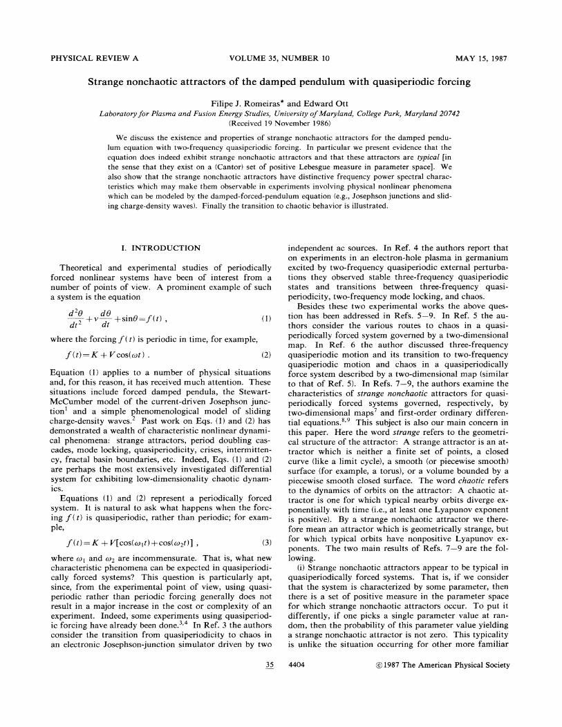
FIG. 1. Diagram of the K-V plane showing regions whereA &0 (hatched) or A=O (blank) (p =3.0). The criterion fornegative Lyapunov exponent is A & —10 . A grid of 201values of K by 66 values of V was used; the integration was tak-en over a variable number of driver periods going fromN =2)& 10 for most cases up to N = 32 && 10' for the more slow-

ly converging ones.

0.8 I.O 1.2 14 1.6 I.B

FIG. 3. Diagram of the K- V plane showing the most impor-tant resonances identified by the triplet (n, l, m) [cf. Eq. (7)](p =3.0).

l mW =—co)+—co2,

n n(7)

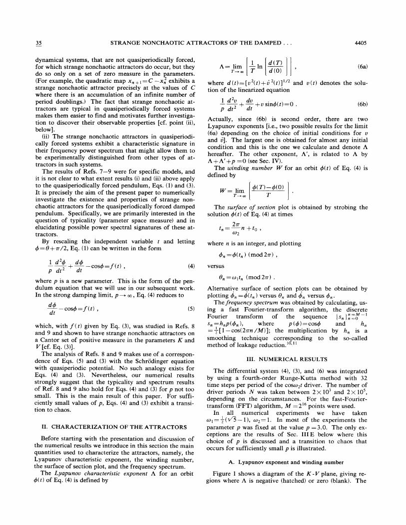
where l, m, n are integers, and between these intervalsthere is a Cantor set on which 8' increases with K. Forsmall K in Fig. 2, A is apparently negative on both theCantor set and the intervals, while for large I|, A is ap-parently zero on the Cantor set and negative on the inter-

criterion for negative Lyapunov exponent used in this fig-ure is A & —10 . The diagram exhibits a structure simi-lar to the Arnold tongues of the circle map (see, for exam-ple, Ref. 12, p. 111).

Figure 2 shows curves of A and W as functions of K ata fixed value of V. The curve of W versus K is apparent-ly a "devil's staircase": a continuous nondecreasing curvewith a dense set of open intervals on which W is constantand given by

vals. The regions where Eq. (7) holds appear in Fig. 1 asthe narrow tongues emerging at small V.

Figure 3 is another diagram of the E-V plane showingthe position of the most prominent plateaus of constantwinding number identified by the triplets (n, l, m). It isclear that the n & 1 plateaus occupy a very small portionof the parameter space.

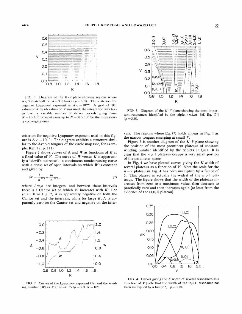
In Fig. 4 we have plotted curves giving the K width ofseveral plateaus as a function of V. Note the scale for then =2 plateau in Fig. 4 has been multiplied by a factor of5. This plateau is actually the widest of the n & 1 pla-teaus. The figure shows that the width of the plateaus in-creases from zero to a maximum value, then decrease topractically zero and then increases again [at least from theevidence of the (1,0, 1) plateau].

0.35

0.30 (1,1,0)

0.0—I I I I I I I I I I I

2.0 0.25

'- I.6 0.20

-0.4 O. I5

—0.6 — 0.8 O. IO

—0.8 —0.4 0.05

— 0.0—1.0 +I I I I I I I I I

0.6 0.8 I.O l.2 l.4 I.6 I.80.0 0.4 0.8 I.2 I.6 2.0

V

FIG. 2. Curves of the Lyapunov exponent (A) and the wind-

ing number ( 8') vs K at V=0.55 (p =3.0, N =10 ).

FIG. 4. Curves giving the K width of several resonances as afunction of V [note that the width of the (2,3,1) resonance hasbeen multiplied by a factor 5) (p =3.0).

35 STRANGE NONCHAOTIC ATTRACTORS OF THE DAMPED. . .

B. Surface of section plots

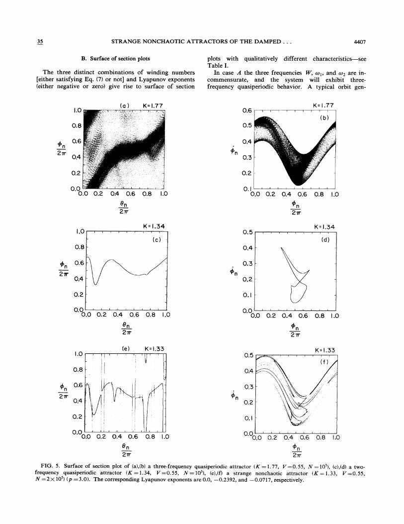
The three distinct combinations of winding numbers[either satisfying Eq. (7) or not] and Lyapunov exponents(either negative or zero) give rise to surface of section

plots with qualitatively different characteristics —seeTable I.

In case A the three frequencies 8' co~, and m2 are in-commensurate, and the system will exhibit three-frequency quasiperiodic behavior. A typical orbit gen-

&n27r

I.O;

0.8

0.2 -.-.-';-=-,.„'-".'=

(a ) K=1.77

h

c

0.64T

'ilhfj I

0.4 ~III I i i

0.3—

0.2—

K= I.77I I I

(b)

ii»'.'

1

.. 'I .' 1' - '»..$. -'. ; ..t0.0 '"

en27r

0.0 0.2 0.4 0.6 0.8 I.O0 I

I I I I I I I I I

0.0 0.2 0.4 0.6 0.8 I.O

n

27r

K = I.34I..0 I I I I I I I I I

(c)0.8—

0.5

0.4—

K =1.34I I I

0.627r

0.4

0.3—

0.2—

0.2— O. I—

I I I I I I I I0. 0.0 0.2 0.4 0.6 0.8 1.0en27r

0..0 I I I I I I I I I

0.0 0.2 0.4 0.6 0.8 1.0

n

27r

I.O(e) K=1.35

' I,'I I I 0.5

K= I.33

0.8— 04

0.6 ):27r

0.4-0.3

n0.2

0.2—i O. I

I

:I 5 1 I I I I I

0.0 0.2 0.4 0.6 O.8 I.O

e„27r

I I I I I I I I I

0.0 0.2 0.4 0.6 0.8 I.p

n

27r

FIG. 5. Surface of section plot of (a),(b) a three-frequency quasiperiodic attractor (~ =1.77, V=0.55, & =10'), (c),(d) a twofrequency quasiperiodic attractor (K = 1.34, V =0.55, N = 10 ), (e),(f) a strange nonchaotic attractor (~ = 1.33, V =0.55,N =2)& 10 ) (p =3.0). The corresponding Lyapunov exponents are 0.0, —0.2392, and —0.0717, respectively.


TABLE I. Characteristics of attractors.

Case

IW& —co)

nl

W =—cg 1

nl

W& —col

n

m+—C02nm+ Cdpn

m+ Cc)2n

Winding number Lyapunov exponent

A&0

A&0

Type of attractor

Three-frequency quasiperiodic

Two-frequency quasiperiodic

Strange nonchaotic

Figure

5(a),5(b)

5(c),5(d)

5(e),5(f)

crates a smooth density of points densely filling the sur-face of section (0,$). This is illustrated in Fig. 5(a). InFig. 5(b) we have also plotted the corresponding surface ofsection (P,P).

In case B the frequency 8 is rationally related to co~

and co2 and the system will exhibit two-frequency quasi-periodic behavior. The attracting orbit in the surface ofsection (0,$) lies on a smooth multivalued curve. If onetakes in Eq. (7) l, n and m, n to be relatively prime in-tegers, then n gives the multiplicity of the curve in thesurface of section. An example of a two-frequency quasi-periodic attractor is given in Fig. 5(c) (note that in thiscase [(n, l, m)=(1,0, 1), to which corresponds 8'= I]. InFig. 5(d) we have plotted the corresponding section in theplane (P,P).

In case C the attractor is geometrically strange: It sat-isfies a functional relationship Q=F(0) but the function Fis discontinuous everywhere. This can be verified in thefollowing way: (i) To verify the existence of the relation-ship Q=F(0) we initialize a large number of points at asingle initial 0 value but with different initial (P,P) valuesand find that after a large number N of co2 periods, all or-bits are attracted to a single pair (tt~, Pz); (ii) thatQ=F(0) cannot be a continuous curve follows if thewinding number W is irrationally related to coI, ruz', (iii) fi-nally, that Q=F(0) is discontinuous everywhere followsfrom the fact that the map 0„+,——0„+2nruI/ru2 (mod 27r)is ergodic. An example of a strange nonchaotic attractoris given in Figs. 5(e) and 5(f).

We note that according to the Kaplan-Yorke formula

K= I.770.~0 ' I I I I I

(a)—I.O—

(f)

0.0

r —I.O-M

K = I.34

-2.0

-3.0O

o 40

-2.0—

-3.0—O

-~.0—

—5.00.0 0. I 0.2 0.3 0.4 0.5

KM

50 I II I'

I I

0.0 O. I 0.2 0.3 0.4 0.5

O.O

—I.O—(/)

K= I.33I I I I I I I I I

(c)

-2.0

-3.0D

o -40

—5.0O.O O. I O. 2 0.3 0.4 0.5

KM

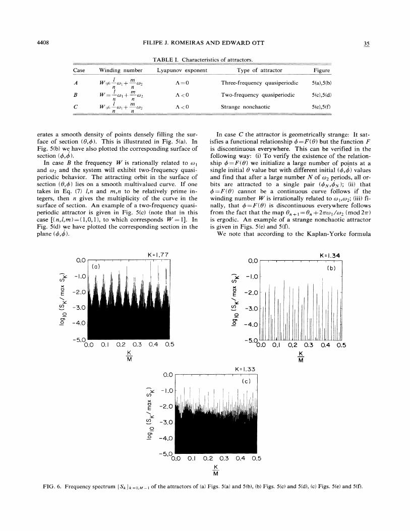
FIG. 6. Frequency spectrum ) Sk )k o M ~ of the attractors of (a) Figs. 5(a) and 5(b), (b) Figs. 5(c) and 5(d), (c) Figs. 5(e) and 5(fI.


5.0 C. Frequency spectral characteristics

4.0-

b 5.0

O2.0

I.O

0.0 -6.0 -4.0 —2.0 0.0log IO0

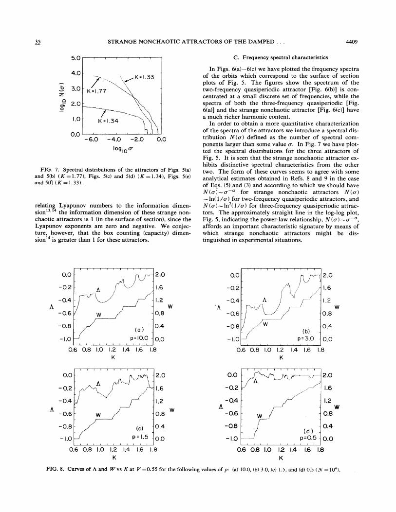
FIG. 7. Spectral distributions of the attractors of Figs. 5(a)and 5(b) (%=1.77), Figs. 5(c) and 5(d) (%=1.34), Figs. 5(e)and 5(f) (K =1.33).

relating Lyapunov numbers to the information dimen-sion' '" the information dimension of these strange non-chaotic attractors is 1 (in the surface of section), since theLyapunov exponents are zero and negative. We conjec-ture, however, that the box counting (capacity) dimen-sion' is greater than 1 for these attractors.

In Figs. 6(a)—6(c) we have plotted the frequency spectraof the orbits which correspond to the surface of sectionplots of Fig. 5. The figures show the spectrum of thetwo-frequency quasiperiodic attractor [Fig. 6(b)] is con-centrated at a small discrete set of frequencies, while thespectra of both the three-frequency quasiperiodic [Fig.6(a)] and the strange nonchaotic attractor [Fig. 6(c)] havea much richer harmonic content.

In order to obtain a more quantitative characterizationof the spectra of the attractors we introduce a spectral dis-tribution N(o. ) defined as the number of spectral com-ponents larger than some value o.. In Fig. 7 we have plot-ted the spectral distributions for the three attractors ofFig. 5. It is seen that the strange nonchaotic attractor ex-hibits distinctive spectral characteristics from the othertwo. The form of these curves seems to agree with someanalytical estimates obtained in Refs. 8 and 9 in the caseof Eqs. (5) and (3) and according to which we should haveN (o)—o . for strange nonchaotic attractors N ( cr )

-ln(1/cr) for two-frequency quasiperiodic attractors, andN(cr) —ln (1/o) for three-frequency quasiperiodic attrac-tors. The approximately straight line in the log-log plot,Fig. 5, indicating the power-law relationship, N (o ) -oaffords an important characteristic signature by means ofwhich strange nonchaotic attractors might be dis-tinguished in experimental situations.

O.O— 2.0 0.0— 2.0

-0.2— — I.6 -0.2—

-0.4 —0.4 — I.2

-0.6 W— 0.8 —0.8

-0.8 (a)— 0.4

—I.O P= IO.O — 0 0I I I I I I I I I I I

0.6 0.8 I.O l.2 l.4 t.6 l.8

-0.8 —0.4—I.O

(b)p=&.o -O.O

I I I I I I I I I I I

0.6 0.8 I.O l.2 l.4 1.6 l.8

0.0 2.0 u 20—0.2 -0.2

-0.4 l.2 — l.2

—0.6 0.8 -06— — 0.8

-0.8 0.4—I.O 0.0


0.6 0.8 I.O l.2 l.4 I.6 l.8

(d)P=0.5 — 0 0


0.6 0.8 l.0 l.2 1.4 l.6 l.8

FIG. 8. Curves of A and W vs E at V =0.55 for the following values of p: (a) 10.0, (b) 3.0, (c) 1.5, and (d) 0.5 ( X = 10 ).


D. Typicality of strange nonchaotic attractors

In the case of Eqs. (5) and (3) a combination of analyti-cal and numerical results indicates that the strange non-chaotic attractors occur on a Cantor set of positive Lebes-gue measure in parameter space. Is this measure still pos-itive in the case of Eqs. (4) and (3) or is it zero? In orderto try to answer this question we have performed the fol-lowing numerical experiment. With the parameters p, Vfixed at the values of Fig. 2 we have taken the set of Avalues

K"=0.685+0.005(i —1), i =1,2, . . . , 49

which lie between the widest plateaus 8 =0.0 andW=co[ (the points K =0.680 and 0.930 are already onthese plateaus, respectively) and for each of these value wecalculated the winding numbers of the orbits with param-eters

equal, we say that K is on a plateau, while if they are dif-ferent, we say that K is on the Cantor set. By proceedingin this way we found that 49 84% of points are on theCantor set. Repeating this study for other small 6 values(b, =4X 10, 16X 10, 64&(10 ), we obtained identicalresults. These results seem to indicate that the measure ofthe Cantor set where the strange nonchaotic attractorsoccur is also positive in the case of the pendulum equa-tion. One observation is in order regarding what we meanby equal and different winding numbers; we found thatthe distinction between the two cases is always very sharp;for points on the plateaus the difference between thewinding numbers is always less than 10, while forpoints on the Cantor set is always larger than 10 . (Thisstrongly suggests that we are not mistaking many closelyspaced narrow plateaus for a Cantor set of positive mea-sure. )

E. Transition to chaos

by integrating Eqs. (4) and (3) over N =10 driver periods.When at least two of these three winding numbers are

In order to illustrate how the parameter p affects thebehavior of the solutions of Eqs. (4) and (3) we have plot-

I.O

.8—

I I I I I I

K = 0.79I I I

(a)0.3 K=0.79

[ I

(b)

n

2m 04

I I I I I ! I ! I

0.0 0.2 0.4 0.6 0.8 I.OQ I

0.0 0.2 0.4 0.6 0.8 I.O

n

27r

4n27r

(c) K =080- 1'1

0.8—(i I

!

!I[

Q Q .1 R ! '0'%& '! '! l' ''' t 'I

0.0 0.2 0.4 0.6 0.8 I.O

K =Q.80I I

(cI)

0.2

Pn Q I—

0.0

Q0.0 0.2 0.4 0.6 0.8 I.O

n2'n

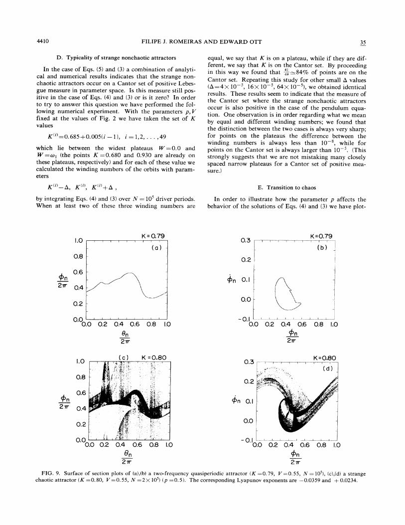
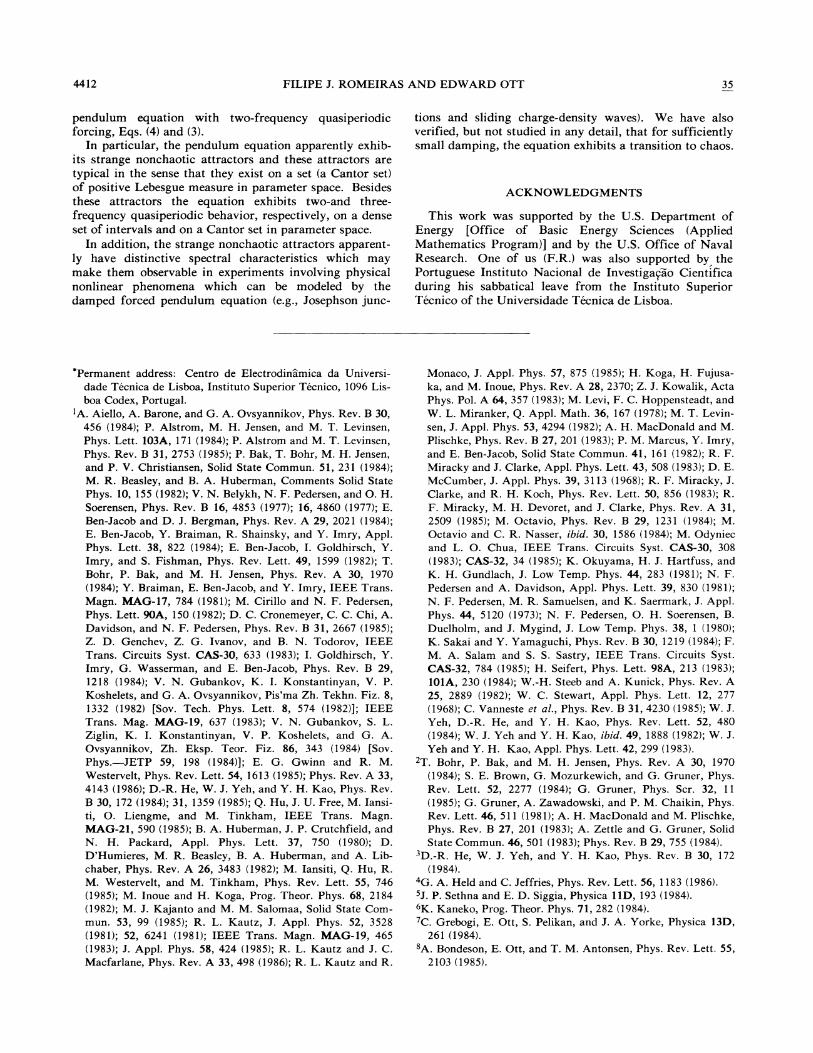
2'FIG. 9. Surface of section p1ots of (a), (b) a two-frequency quasiperiodic attractor (K =0.79, V=0.55, N =10'), (c),(d) a strange

chaotic attractor (K =0.80, V =0.55, N =2&(10 ) (p =0.5). The corresponding Lyapunov exponents are —0.0359 and + 0.0234.


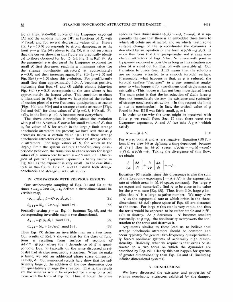
ted in Figs. 8(a)—8(d) curves of the Lyapunov exponent(A) and the winding number ( 8') as functions of K, withV fixed, and for several decreasing values of p. Figure8(a) (p =10.0) corresponds to strong damping; as in thelimit p~ m Eq. (4) reduces to Eq. (5), it is not surprisingthat the curves shown in this figure are practically identi-cal to those obtained for Eq. (5) (cf. Fig. 2 in Ref. 9). Asthe parameter p is decreased the Lyapunov exponent forsmall K first decreases, reaching a minimum value (forthe strange nonchaotic attractors) at approximatelyp =3.0, and then increases again; Fig. 8(b) (p =3.0) andFig. 8(c) (p =1.5) show this evolution. For p sufficientlysmall (less than approximately 1.0), A becomes positive,indicating that Eqs. (4) and (3) exhibit chaotic behavior;Fig. 8(d) (p =0.5) corresponds to the case where A hasapproximately the largest value. This transition to chaosis illustrated in Fig. 9 where we have plotted the surfaceof section plots of a two-frequency quasiperiodic attractor[Figs. 9(a) and 9(b)] and a strange chaotic attractor [Figs.9(c) and 9(d)] for close values of E (p =0.5, V fixed). Fi-nally, in the limit p ~0, A becomes zero everywhere.

The above description is mainly about the evolutionwith p of the A versus K curve for small values of K, thatis, for values of K for which in the large-p limit strangenonchaotic attractors are present; we have seen that as pdecreases below a certain value (p=1.0) these strangenonchaotic attractors disappear in favor of strange chaot-ic attractors. For large values of K, for which in thelarge-p limit the system exhibits three-frequency quasi-periodic behavior, the transition to chaos occurs for largervalues of p (somewhere between p =2.5 and 3.0). This re-gion of positive Lyapunov exponent is barely visible inFig. 8(c), as the exponent is very small. In the case illus-trate in this figure, Eqs. (5) and (3) exhibit both strangenonchaotic and strange chaotic attractors.

0„+~ =(0„+2vr/co&) (mod 2') . (8b)

Formally setting p = co, Eq. (4) becomes Eq. (5), and thecorresponding invertible map is two dimensional,

P„+,——g($„,9„) (mod2vr), (9a)

0„+~

——(0„+2~/co2) (mod 2') . (9b)

Thus Eqs. (9) define an invertible map on a two torus.Our results of Ref. 9 showed that for the class of func-tions g resulting from surface of sections ofdP/dt =g(P, t) where the t dependence of g is quasi-periodic, Eqs. (9) typically (in the sense discussed previ-ously) had strange nonchaotic attractors. When we makep finite, we add an additional phase space dimension,namely, P. Our numerical results here show that for suf-ficiently large p, the addition of the new dimension doesnot qualitatively change the situation. That is, the resultsare the same as would be expected for a map on a twotorus with the form of Eqs. (9). Thus, although the phase

IV. COMPARISON WITH PREVIOUS RESULTS

Our stroboscopic sampling of Eqs. (4) and (3) at thetimes t =t„=2m.n /co2+ta defines a three-dimensiona1 in-vertible map,

(4.+i 4.+»=G(4. 0. ~.» (8a)

space is four dimensional (Q, Q, 0=co, t, g=cozt), it is ap-parently the case that there is an embedded three torus towhich all orbits are attracted, and on which (with somesuitable change of the P coordinate) the dynamics isdescribed by an equation of the form dP/dt =g(P, t). Itis on this torus that the quasiperiodic and strange non-chaotic attractors of Figs. 5 lie. No chaos with positiveLyapunov exponent is possible as long as this situation ap-plies [it is ruled out for Eqs. (9) with invertible g]. Ourtransition to chaos (Sec. IIIE) means that the solutionsare no longer attracted to a smooth toroidal surface.Presumably, what happens is that, as p is reduced, thetoroidal surface "fractures" in a way somewhat analo-gous to what happens for two-dimensional circle maps atcriticality. (This, however, has not been investigated here. )

The main point is that the introduction oi finite large pdoes not immediately destroy the existence and typicalityof strange nonchaotic attractors. (In this respect the limitp~~ is nonsingular. ) In fact, the critical value of pfound in Sec. III E was fairly small, p, =1.

In order to see why the torus might be preserved withfinite p we recall from Sec. II that there were twoLyapunov exponents, A and A' (we take A & A') whichsatisfy

A'= —(p+A) . (10)

a dj adt BP dt

+

Equation (10) results, since this divergence is also the sumof the Lyapunov exponents [—(A+A') is the exponentialrate at which areas in (P,P) space, contract]. For large pwe expect and numerically find A to be close to its valuefor the p = oo case [Eq. (5)]. Thus from (10), large p im-plies that A' is a large negative number. We may view—A' as the exponential rate at which orbits in the three-dimensional ($,$,0) phase space of Eqs. (8) are attractedto the torus. For large p this rate is very rapid, and thusthe torus would be expected to be rather stable and diffi-cult to destroy. As p decreases —A' becomes smaller;eventually, at p =p„ the nonlinearity overpowers the con-traction to the torus and destroys it.

Arguments similar to these lead us to believe thatstrange nonchaotic attractors should be common andoccur typically for general two-frequency quasiperiodical-ly forced nonlinear systems of arbitrarily high dimen-sionality. Basically, what we require is that orbits be at-tracted to a two torus on which the dynamics aredescribed by Eqs. (9). Clearly this can happen for systemsof greater dimensionality than Eqs. (3) and (4) (includinginfinite dimensional systems).

V. CONCLUSIONS

We have discussed the existence and properties ofstrange nonchaotic attractors exhibited by the damped

For p & p, both A and A' are negative. Equation (10) fol-lows if we view (4) as defining a time dependent fbecauseof f ( t)] flow in (P,P) space, dP/dt = —p (P —cosP)+f(t), dP!dt =P. Taking the divergence of this flow,we obtain


pendulum equation with two-frequency quasiperiodicforcing, Eqs. (4) and (3).

In particular, the pendulum equation apparently exhib-its strange nonchaotic attractors and these attractors aretypical in the sense that they exist on a set (a Cantor set)of positive Lebesgue measure in parameter space. Besidesthese attractors the equation exhibits two-and three-frequency quasiperiodic behavior, respectively, on a denseset of intervals and on a Cantor set in parameter space.

In addition, the strange nonchaotic attractors apparent-ly have distinctive spectral characteristics which maymake them observable in experiments involving physicalnonlinear phenomena which can be modeled by thedamped forced pendulum equation (e.g. , Josephson junc-

tions and sliding charge-density waves). We have alsoverified, but not studied in any detail, that for sufficientlysmall damping, the equation exhibits a transition to chaos.

ACKNOWLEDGMENTS

This work was supported by the U.S. Department ofEnergy [Office of Basic Energy Sciences (AppliedMathematics Program)] and by the U.S. Office of NavalResearch. One of us (F.R.) was also supported by thePortuguese Instituto Nacional de Investigaqao Cientificaduring his sabbatical leave from the Instituto SuperiorTecnico of the Universidade Tecnica de Lisboa.

'Permanent address: Centro de Electrodinamica da Universi-dade Tecnica de Lisboa, Instituto Superior Tecnico, 1096 Lis-boa Codex, Portugal ~

A. Aiello, A. Barone, and G. A. Ovsyannikov, Phys. Rev. B 30,456 (1984); P. Alstrom, M. H. Jensen, and M. T. Levinsen,Phys. Lett. 103A, 171 (1984); P. Alstrom and M. T. Levinsen,Phys. Rev. 8 31, 2753 (1985); P. Bak, T. Bohr, M. H. Jensen,and P. V. Christiansen, Solid State Commun. 51, 231 (1984);M. R. Beasley, and B. A. Huberman, Comments Solid StatePhys. 10, 155 (1982); V. N. Belykh, N. F. Pedersen, and O. H.Soerensen, Phys. Rev. B 16, 4853 (1977); 16, 4860 (1977); E.Ben-Jacob and D. J. Bergman, Phys. Rev. A 29, 2021 (1984);E. Ben-Jacob, Y. Braiman, R. Shainsky, and Y. Imry, Appl.Phys. Lett. 38, 822 (1984); E. Ben-Jacob, I. Goldhirsch, Y.Imry, and S. Fishman, Phys. Rev. Lett. 49, 1599 (1982); T.Bohr, P. Bak, and M. H. Jensen, Phys. Rev. A 30, 1970(1984); Y. Braiman, E. Ben-Jacob, and Y. Imry, IEEE Trans.Magn. MAO-17, 784 (1981); M. Cirillo and N. F. Pedersen,Phys. Lett. 90A, 150 (1982); D. C. Cronemeyer, C. C. Chi, A.Davidson, and N. F. Pedersen, Phys. Rev. B 31, 2667 (1985);Z. D. Genchev, Z. G. Ivanov, and B. N. Todorov, IEEETrans. Circuits Syst. CAS-30, 633 (1983); I. Goldhirsch, Y.Imry, G. Wasserman, and E. Ben-Jacob, Phys. Rev. B 29,1218 (1984); V. N. Gubankov, K. I. Konstantinyan, V. P.Koshelets, and G. A. Ovsyannikov, Pis'ma Zh. Tekhn. Fiz. 8,1332 (1982) [Sov. Tech. Phys. Lett. 8, 574 (1982)]; IEEETrans. Mag. MACx-19, 637 (1983); V. N. Gubankov, S. L.Ziglin, K. I. Konstantinyan, V. P. Koshelets, and G. A.Ovsyannikov, Zh. Eksp. Teor. Fiz. 86, 343 (1984) [Sov.Phys. —JETP 59, 198 (1984)]; E. G. Cxwinn and R. M.Westervelt, Phys. Rev. Lett. 54, 1613 (1985); Phys. Rev. A 33,4143 (1986); D.-R. He, W. J. Yeh, and Y. H. Kao, Phys. Rev.B 30, 172 (1984); 31, 1359 (1985); Q. Hu, J. U. Free, M. Iansi-ti, O. Liengme, and M. Tinkharn, IEEE Trans. Magn.MAG-21, 590 (1985); B. A. Huberman, J. P. Crutchfield, andN. H. Packard, Appl. Phys. Lett. 37, 750 (1980); D.D'Humieres, M. R. Beasley, B. A. Huberman, and A. Lib-chaber, Phys. Rev. A 26, 3483 (1982); M. Iansiti, Q. Hu, R.M. Westervelt, and M. Tinkham, Phys. Rev. Lett. 55, 746(1985); M. Inoue and H. Koga, Prog. Theor. Phys. 68, 2184(1982); M. J. Kajanto and M. M. Salomaa, Solid State Com-mun. 53, 99 (1985); R. L. Kautz, J. Appl. Phys. 52, 3528(1981); 52, 6241 (1981); IEEE Trans. Magn. MAG-19, 465(1983); J. Appl. Phys. 58, 424 (1985); R. L. Kautz and J. C.Macfarlane, Phys. Rev. A 33, 498 (1986); R. L. Kautz and R.

Monaco, J. Appl. Phys. 57, 875 (1985); H. Koga, H. Fujusa-ka, and M. Inoue, Phys. Rev. A 28, 2370; Z. J. Kowalik, ActaPhys. Pol. A 64, 357 (1983); M. Levi, F. C. Hoppensteadt, andW. L. Miranker, Q. Appl. Math. 36, 167 (1978); M. T. Levin-sen, J. Appl. Phys. 53, 4294 (1982); A. H. MacDonald and M.Plischke, Phys. Rev. B 27, 201 (1983); P. M. Marcus, Y. Imry,and E. Ben-Jacob, Solid State Commun. 41, 161 (1982); R. F.Miracky and J. Clarke, Appl. Phys. Lett. 43, 508 (1983); D. E.McCumber, J. Appl. Phys. 39, 3113 (1968); R. F. Miracky, J.Clarke, and R. H. Koch, Phys. Rev. Lett. 50, 856 (1983); R.F. Miracky, M. H. Devoret, and J. Clarke, Phys. Rev. A 31,2509 (1985); M. Octavio, Phys. Rev. B 29, 1231 (1984); M.Octavio and C. R. Nasser, ibid. 30, 1586 (1984); M. Odyniecand L. O. Chua, IEEE Trans. Circuits Syst. CAS-30, 308(1983); CAS-32, 34 (1985); K. Okuyama, H. J. Hartfuss, andK. H. Gundlach, J. Low Temp. Phys. 44, 283 (1981); N. F.Pedersen and A. Davidson, Appl. Phys. Lett. 39, 830 (1981);N. F. Pedersen, M. R. Samuelsen, and K. Saermark, J. Appl.Phys. 44, 5120 (1973); N. F. Pedersen, O. H. Soerensen, B.Duelholm, and J. Mygind, J. Low Temp. Phys. 38, 1 (1980);K. Sakai and Y. Yarnaguchi, Phys. Rev. B 30, 1219 (1984); F.M. A. Salam and S. S. Sastry, IEEE Trans. Circuits Syst.CAS-32, 784 (1985); H. Seifert, Phys. Lett. 98A, 213 (1983);101A, 230 (1984); W.-H. Steeb and A. Kunick, Phys. Rev. A25, 2889 (1982); W. C. Stewart, Appl. Phys. Lett. 12, 277(1968); C. Vanneste et al. , Phys. Rev. B 31, 4230 (1985); W. J.Yeh, D.-R. He, and Y. H. Kao, Phys. Rev. Lett. 52, 480(1984); W. J. Yeh and Y. H. Kao, ibid. 49, 1888 (1982); W. J.Yeh and Y. H. Kao, Appl. Phys. Lett. 42, 299 (1983).

2T. Bohr, P. Bak, and M. H. Jensen, Phys. Rev. A 30, 1970(1984); S. E. Brown, G. Mozurkewich, and G. Gruner, Phys.Rev. Lett. 52, 2277 (1984); G. Gruner, Phys. Scr. 32, 11(1985); G. Gruner, A. Zawadowski, and P. M. Chaikin, Phys.Rev. Lett. 46, 511 (1981);A. H. MacDonald and M. Plischke,Phys. Rev. B 27, 201 (1983); A. Zettle and G. CJruner, SolidState Commun. 46, 501 (1983); Phys. Rev. B 29, 755 (1984).

3D.-R. He, W. J. Yeh, and Y. H. Kao, Phys. Rev. B 30, 172(1984).

4G. A. Held and C. Jeffries, Phys. Rev. Lett. 56, 1183 (1986).5J. P. Sethna and E. D. Siggia, Physica 11D, 193 (1984).K. Kaneko, Prog. Theor. Phys. 71, 282 (1984).

7C. Grebogi, E. Ott, S. Pelikan, and J. A. Yorke, Physica 13D,261 (1984).

8A. Bondeson, E. Ott, and T. M. Antonsen, Phys. Rev. Lett. 55,2103 (1985).

35 STRANCyE NONCHAOTIC ATTRACTORS OF THE DAMPED. . . 4413

F. J. Romeiras, A. Bondeson, E. Ott, T. M. Antonsen, and C.Grebogi, Physica D (to be published).E. O. Brigham, The Fast Fourier Transform (Prentice-Hall,Englewood Cliffs, N.J., 1974).

Cx. E. Powell and I. C. Percival, J. Phys. A 12, 2053 (1979).~~R. L. Devaney, An Introduction to Chaotic Dynamical Systems

(Benjamin/Cummings, Menlo Park, CA. , 1986).~3J. Kaplan and J. A. Yorke, Functional Differentia! Equations

and the Approximation of Fixed Points (Springer, Berlin,1978), p. 228.

J. D. Farmer, E. Ott, and J. A. Yorke, Physica 7D, 153 (1983).

Documents

Strange nonchaotic attractors of the damped pendulum with quasiperiodic forcing