Embed Size (px)
Citation preview
Int. J. Product Lifecycle Management, Vol. X, No. Y, xxxx 1
Copyright © 200x Inderscience Enterprises Ltd.
Strategic management of component obsolescence using constraint-driven design refresh planning
Raymond S. Nelson III and Peter Sandborn* CALCE Center for Advanced Life Cycle Engineering, Department of Mechanical Engineering, University of Maryland, College Park, MD 20742, USA E-mail: [email protected] E-mail: [email protected] *Corresponding author
Abstract: Technology obsolescence also known as diminishing manufacturing sources and material shortages (DMSMS) is a significant problem for systems whose operational life is much longer than the procurement lifetimes of their constitute components. The most severely affected systems are sustainment-dominated, which means their long-term sustainment (lifecycle) costs significantly exceed the procurement cost of the system. Unlike high-volume commercial products, these sustainment-dominated systems may require design refreshes to simply remain manufacturable and supportable. Design refresh planning (DRP) is a strategic method for reducing the lifecycle cost impact of DMSMS and increasing system availability. The objective of DRP is to determine when a design refresh should occur (or what the frequency of refreshes should be) and how to manage the system components that are obsolete or soon to be obsolete at the design refreshes. This paper describes the formulation and implementation of constraints in the DRP process for systems impacted by DMSMS type obsolescence and proposes a method of transforming an implicit system limitation into an explicit DRP constraint. These constraints can reflect technology roadmap requirements, obsolescence management realities, logistics limitations, budget limitations and management policy.
Keywords: component obsolescence; product lifecycle management; diminishing manufacturing sources and material shortages; DMSMS; design refresh plan; DRP; constraint-driven; cost; sustainment.
Reference to this paper should be made as follows: Nelson, R.S. III and Sandborn, P. (xxxx) ‘Strategic management of component obsolescence using constraint-driven design refresh planning’, Int. J. Product Lifecycle Management, Vol. X, No. Y, pp.000–000.
Biographical notes: Raymond S. Nelson III is a Researcher at the Center for Advanced Life Cycle Engineering (CALCE) in the University of Maryland, College Park. His research interests mainly focus on strategic design refresh planning, lifecycle cost modelling, hardware and software coupled obsolescence, and obsolescence information modelling.
Peter Sandborn is a Professor in the CALCE Electronic Products and Systems Center at the University of Maryland. His group develops obsolescence forecasting algorithms, performs strategic design refresh planning, and lifetime buy quantity optimisation. He is the developer of the MOCA refresh planning tool. MOCA has been used by private and government organisations worldwide
2 R.S. Nelson III and P. Sandborn
to perform optimised refresh planning for systems subject to technology obsolescence. He also performs research in several other lifecycle cost modelling areas including maintenance planning and return on investment analysis for the application of prognostics and health management (PHM) to systems, total cost of ownership of electronic parts, transition from tin-lead to lead-free electronics, and general technology trade-off analysis for electronic systems.
1 Introduction
Technology obsolescence is defined as the loss or impending loss of original manufacturers of items or suppliers of items or raw materials (Sandborn, 2008). The type of obsolescence addressed in this paper is referred to as diminishing manufacturing sources and material shortages (DMSMS) and is caused by the unavailability of technologies or components that are needed to manufacture or sustain a product. In this paper, ‘component’ refers to the lowest management level possible for the system being analysed. In some systems, the ‘components’ are laptop computers, operating systems, and cables; while in other systems the components are integrated circuits (chips). DMSMS means that due to the length of the system’s manufacturing and support life, coupled with unforeseen support life extensions, needed components become unavailable (or at least unavailable from their original manufacturer) before the system’s demand for them is exhausted.1 Component unavailability from the original manufacturer means an end of production and/or support for the component. Components may become obsolete for a variety of reasons that include: the introduction of newer replacement components, dwindling market share, corporate acquisitions and mergers, changes in legislation, and the disruption of supply chains due to natural disasters and other causes.2 It is possible for aftermarket suppliers to continue to sell a component after obsolescence; however, not all components are available in the aftermarket and buying components in the aftermarket is expensive and introduces additional risks that may be unacceptable for many types of systems, e.g., counterfeit risk (Pecht and Tiku, 2006).
The DMSMS type obsolescence problem is especially prevalent in ‘sustainment-dominated’ systems where the cost of sustaining (maintaining) the system over its support life far exceeds the cost of manufacturing or procuring the system (Sandborn and Myers, 2008). Sustainment in this paper refers to three things: keeping the system operational, continuing to manufacture and install versions of the original system that satisfy the original requirements, and finally the ability to manufacture and install versions of the original system that satisfy new and evolving requirements. Examples of sustainment-dominated systems include airplanes, military systems, telecommunications infrastructure, and other infrastructure-, safety- and mission- critical systems. These types of systems are produced at low volumes compared to commercial products such as personal computers or cell phones, which means that they have little to no control over their supply chains. They also have long enough design cycles that a significant portion of the technology in them may be obsolete prior to the system being fielded for the first time. Once in the field, their operational support can be 30 years or more (Tomczykowski, 2003). For these systems, simply replacing obsolete components with newer components is often not a viable solution because of high reengineering costs and
Strategic management of component obsolescence 3
the prohibitive cost of system re-qualification and re-certification. For example, if an electronic component in the 25-year-old control system of a nuclear power plant fails, an instance of the original component may have to be used to replace it so as to not jeopardise the ‘grandfathered’ certification of the plant.
The escalating impact of DMSMS type obsolescence on systems has resulted in the development of a growing number of methodologies, databases and tools that address the obsolescence status of components, forecast future obsolescence risk and provide DMSMS mitigation and management support.
The effective long-term management of DMSMS in systems requires addressing the problem on three different management levels: reactive, pro-active and strategic. The reactive management level is concerned with determining an appropriate, immediate resolution to the problem of components becoming obsolete, executing the resolution process and documenting/tracking the actions taken. Common reactive DMSMS management approaches include: lifetime buy, bridge buy, component replacement, buying from aftermarket sources, up rating, emulation, and salvage (Stogdill, 1999). For example, lifetime buy refers to buying enough components from the original manufacturer prior to the component’s discontinuance to support all forecasted future manufacturing and support needs, and bridge buy means buying a sufficient number of components to reach a pre-determined future date when the component will be designed out of the system.
Pro-active management means that critical components that:
a have a risk of going obsolete
b lack sufficient available quantity after obsolescence
c will be problematic to manage if/when they become obsolete
are identified and managed prior to their actual obsolescence event. Pro-active management requires an ability to forecast obsolescence risk for
components. It also requires that there be a process for articulating, reviewing and updating the system-level DMSMS status.
Strategic management of DMSMS means using DMSMS data, logistics management inputs, technology forecasting, and business trending to enable strategic planning, lifecycle optimisation, and long-term business case development for the support of systems. The most common approach to DMSMS strategic management is design refresh planning (DRP), which consists of choosing the best mix of reactive management approaches such as bridge buys, and design refreshes. A design refresh is a change to the system that is required in order for the system to remain sustainable.
This paper describes the formulation and handling of constraints in the DRP process for systems impacted by DMSMS type obsolescence. In the next section, the DRP methodology is briefly reviewed followed by proposal description of a method used to transform implicit system limitations into explicit constraints for the DRP process. An algorithm used to construct the constraints is provided and demonstrated on an example electronic system DRP problem.
4 R.S. Nelson III and P. Sandborn
2 Design refresh planning
The objective of DRP is to determine when design refreshes should occur so that the lifecycle costs (LCCs) of the system are minimised. The simplest DRP solutions calculate the net present value (NPV) of bridge buys and design refreshes as a function of the date of the design refresh. As a design refresh is delayed, its NPV decreases and the quantity (and thereby cost) of bridge buys required to sustain the system until the design refresh takes place increases (Cattani and Souza, 2003; Porter, 1998).
Value is usually gained from the DRP models through the identification of cost avoidance opportunities (opportunities to avoid future sustainment costs) associated with optimal planning of refreshes (optimal set of refresh dates or the optimal frequency to refresh a system); optimal mixing of reactive DMSMS mitigation solutions with design refreshes, or by identifying refresh points early enough that appropriate budgets and resources can be put in place.
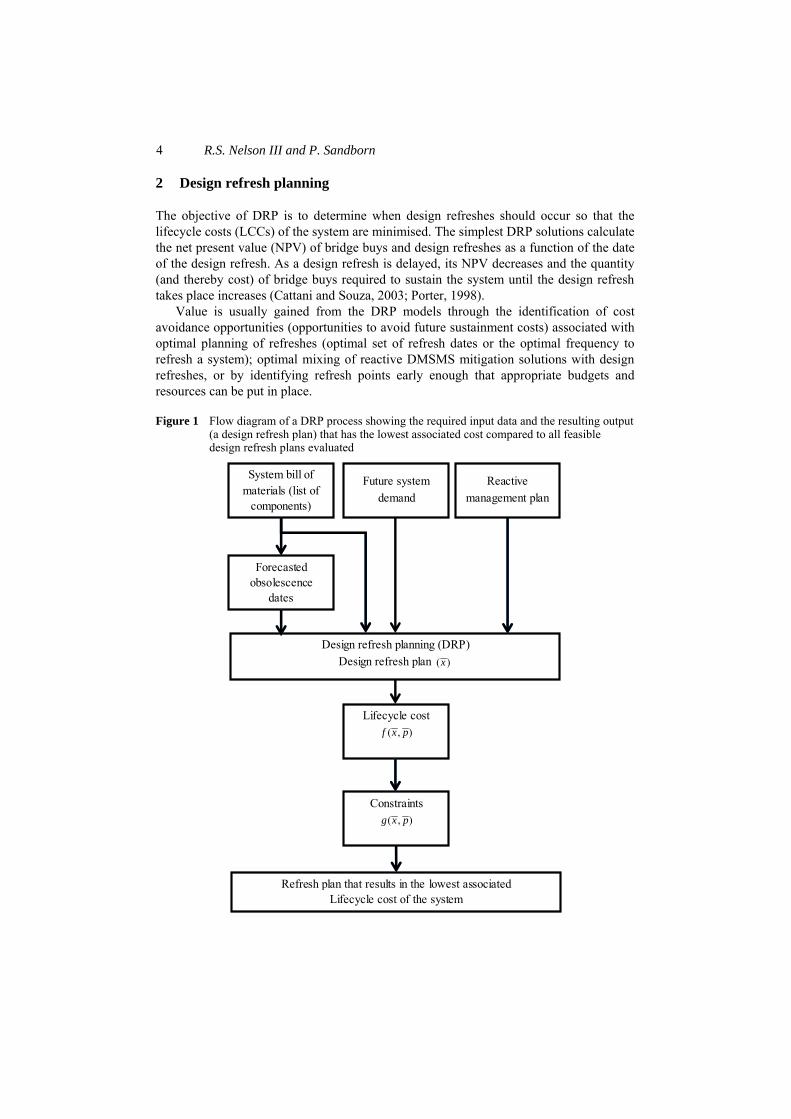
Figure 1 Flow diagram of a DRP process showing the required input data and the resulting output (a design refresh plan) that has the lowest associated cost compared to all feasible design refresh plans evaluated
Refresh plan that results in the lowest associated Lifecycle cost of the system
Constraints ( , )g x p
Lifecycle cost( , )f x p
Design refresh planning (DRP)Design refresh plan ( )x
System bill of materials (list of
components)
Forecasted obsolescence
dates
Future system demand
Reactive management plan
Strategic management of component obsolescence 5
Figure 1 identifies the inputs and outputs of the DRP process. The four main inputs to the DRP process are the bill of materials (BOM) of the system being managed, the forecasted obsolescence dates for the components in the BOM, the future demand for the system being produced and sustained, and the reactive management plan. The system BOM contains component-specific information such as component quantity and cost.3 The BOM is also the input to a procurement life forecasting method, the output of which is obsolescence dates for all the components in the BOM. The forecasted obsolescence dates are then input into the DRP process. The remaining input to the DRP process is the reactive management plan that details how reactive management approaches will be used between design refreshes. The DRP process then calculates a LCC for various combinations of design refresh dates and selects the design refresh plan that has the lowest associated LCC.
The DRP problem can be formulated as shown in equation (1).
minimise ( , )
subject to: ( , ) 0; 1, ,k
f x px
g x p k K≤ = … (1)
The objective function, ( , )f x p calculates the LCC for the system being modelled. The LCC objective function is dependent on 1[ , , ],rx x x= … which is the design variable vector, and 1[ , , ],mp p p= … which is the set of parameters. The design variable is a vector of zero or more design refresh dates representing one design refresh plan. The parameters used in the LCC objective function are constants that do not change during the DRP process such as the production schedule, forecast obsolescence dates, costs for different DRP activities. Since the values used in the design variable vector and the set of parameters represent monetary and quantitative amounts, x and p are restricted to real values.
The LCC objective function is shown in equation (2) (Singh and Sandborn, 2006).
1 1
( , )1 1
100 100
i j
n rji i i i
d di j
NREQ C c qf x pR R= =
+= +
⎛ ⎞ ⎛ ⎞+ +⎜ ⎟ ⎜ ⎟⎝ ⎠ ⎝ ⎠
∑ ∑ (2)
where
Qi quantity of systems to be manufactured at the ith manufacturing event to satisfy demand
qi quantity of spare components to be manufactured at the ith manufacturing event to satisfy demand
Ci recurring cost of manufacturing a system instance at the ith manufacturing event
ci recurring cost of manufacturing a spare component instance at the ith manufacturing event
NREj non-recurring cost of the jth design refresh
n number of manufacturing events
6 R.S. Nelson III and P. Sandborn
r number of design refreshes in the plan
R after tax discount rate on money
d difference in years between event date and the NPV calculation date.
Notice that in equation (2) there are sub-functions that are dependent on the design variable vector, x such as the non-recurring cost, NREj function that gives the non-recurring cost of the jth design refresh, xj. In addition, the parameter set p contains all of the constants shown in equation (2) such as the discount rate, R.
The ( , )f x p LCC objective function, which is a representation of the DRP methodology has the design variable x and parameter set p as its inputs; however, the DRP methodology goes through many intermediate variables in order to calculate a LCC. An example of an intermediate variable is an annual design refresh cost variable (i.e., the amount of money that was spent on all design refreshes within a particular year). While not part of the design variable, these intermediate variables may have constraints placed on them. For example, let there be an annual budget constraint that imposes a million dollar upper bound limit on the annual design refresh cost in year t of the analysis period. The annual budget constraint would then be represented as ( , ) ( , , ) 1,000,000 0.g x p c x p t= − ≤ Taking constraints imposed on intermediate variables and deriving them in terms of the design variable is not possible for all cases.
Constraints imposed in the DRP process can reflect legislative policies, budget realities, technology upgrade roadmaps, logistic limitations, and obsolescence management limitations (Nelson et al., 2011). For the approach presented in this paper the constraints can be characterised by three general types: budgetary, logistical, and temporal. For example, a budgetary constraint may place an upper bound on the money available to perform design refreshes or other management activities in a particular period of time as in the example above. A logistical constraint would restrict the number of components that can be stored for lifetime buys, or limit the number of facilities performing design refreshes (e.g., a finite number of dry docks for ships). Temporal constraints will require the design refresh activity to complete within a specific period of time for technology insertion to upgrade a system’s capability, or may preclude specific periods of time for design refresh because the system to be refreshed is unavailable (e.g., a submarine is gone for 12 months and the design refresh cannot be performed at sea). It should be noted that since the design variable in the DRP process is a list of design refresh dates, the temporal constraints do not require any kind of modification whereas the budget and resource constraints do require a transformation into a constraint that is in terms of the design variable (i.e., design refresh dates). This paper will focus on temporal constraints and specifically their application to electronic systems. For the DMSMS affected systems, temporal constraints are the most prevalent DRP drivers.
Temporal constraints usually take the form of inclusive4 inequalities because they represent ranges of time when at least one design refresh is required. These constraints are typically centred on events such as obsolescence events, legislation enactment events, changes in standards event, etc., because a large majority of system limitations are focused on mitigating the impacts of those events.
The creation of a temporal constraint for a given system is achieved by understanding how the limitations of a system relate to the system’s components within the perspective of the DRP process managing a sustainment-dominated system. Essentially, system
Strategic management of component obsolescence 7
limitations need to be transformed into an explicit form that can be directly imposed on the DRP design variable.
The task of translating system limitations into explicit constraints is challenging when limitations are implicit such as when the limitations are in the form of a policy. A policy provides generalised information on how a system is restricted. For example, an electronic data security policy might state “No software is allowed to operate without security patch support from the OEM software company”. In deciphering this policy, the first step is to identify the component being restricted by this limitation, which could be any and all software within the system. The second step is determining how this limitation restricts the scheduling of a design refresh. When viewing this policy through a DRP process perspective, it is clear that the policy does not explicitly state how it will restrict the scheduling of design refreshes; however, it does reveal three pieces of information that can be used to form the constraint:
1 the component obsolescence occurs when the ‘support’ for the software expires
2 the constraint is permission-based (i.e., ‘is allowed’ refers to the consent from an authoritative actor ‘to operate’ if certain conditions are met) meaning the obsolescence event of a component does not affect the functionality of the system; however, other risks, vulnerabilities, and penalties might be incurred if the constraint is not met
3 the constraint affects the operation of the system, which means the production of the system is also affected by the constraint.
The electronic data security policy example has been broken down into elements that can be used to form the explicit DRP constraint; but before forming the constraint a brief review of some terms is necessary.
Recalling the definition of sustainment-dominated mentioned earlier, the main activities of sustaining a system are ensuring the continued operation and production of a system. These two activities are governed by whether the organisation responsible for sustaining the system has the ability and/or the permission to perform such activities. The ability to perform an activity is based on physical parameters such as the available funds, resources, and time. Permission to perform an activity is based on the authorisation from imposed written law, supervisory actors (e.g., company management, business owner), applicable national/international standards and specifications, and contractual commitments.
Next, the form of the temporal constraint will be determined. It was mentioned before that the budgetary and logistical constraints require a transformation such that the constraint is in terms of the design variable whereas the temporal constraints do not. Budgetary and logistical constraints usually take the form of thresholds and those thresholds are known at the beginning of the DRP process. Temporal constraints are usually bounded ranges of time that require one or more design refresh activities to complete within them; however, those bounds are unknown at the beginning of the DRP process. In order to determine the temporal constraint bounds, it needs to be established whether according to the limitation if the component’s obsolescence event the constraint:
1 affects both the operation and the production of the system
2 affects production and not operation
3 does not affect either activity.
8 R.S. Nelson III and P. Sandborn
It will be assumed that if the component’s obsolescence event affects the operation of the system then the production of the system is also affected. Knowing how the component’s obsolescence event according to the limitation affects the operation and production of a system will determine if and how an explicit constraint will be constructed. The three possible situations called obsolescence event types have been identified, their definitions follow.
In the following obsolescence event type definitions, the term obsolete can take on several meanings depending on the component restricted by the limitations. If the component is a piece of hardware, obsolete generally means you cannot procure the item from the original manufacturer; however, in some cases the item may remain available from your existing inventory or through aftermarket sources. If the component is a single legal copy of software, obsolete usually means you cannot receive software updates such as service packages or security patches.
2.1 ‘Weak’ obsolescence event
No change to previously fielded (installed) systems or systems to be manufactured in the future is required. As long as the obsolete item is available (from existing stock or aftermarket sources), new systems can be manufactured and fielded using it and previously installed systems can be repaired with it if necessary.
System limitations often identify hardware (electronic components for our applications) as having a Weak obsolescence event. The rationale behind this is that if hardware goes obsolete there is no reason to change it as long as you have access to a sufficient supply of the obsolete component to satisfy manufacturing and support requirements.
2.2 ‘Strong A’ obsolescence event
Fielded (installed) systems can continue to operate with the obsolete item and can be replaced with the obsolete item if it needs replacement due to a failure of the item. However, new systems to be manufactured in the future cannot be built and fielded with the obsolete item (whether the obsolete item is available or not).
A recent example of a system limitation that resulted in an organisation identifying a component’s obsolescence event as ‘Strong A’ was caused by the European legislation called the restriction of hazardous substances (RoHS) Directive (Directive 2002/95/EC, 2003). This legislation regulates many of the commonly used substances in electronics and restricts the use of several materials deemed hazardous by the European Union (EU). The most problematic material for electronic systems is lead, which historically is a primary ingredient in solder. The legislation only pertains to electronic systems sold in the EU after July 1, 2006 so any previously fielded systems with non-compliant electronic components are allowed to continue operating; however, new instances of the system to be manufactured and sold in the EU must comply with the RoHS directive by ensuring that every component and subsystem is RoHS compliant regardless of the availability of non-compliant components.
Strategic management of component obsolescence 9
2.3 ‘Strong B’ obsolescence event
Fielded (installed) systems are not allowed to continue to operate with the obsolete item and must be backfitted within a defined time period. New systems cannot be built and fielded with the obsolete item (whether the obsolete item is available or not).
An example of a system limitation that identifies a component’s obsolescence event as ‘Strong B’ is an electronic data security policy. Consider a ship-board communication system that has computers on its network that is connected to the public web running a commercial operating system that is about to reach its end of support date (the effective obsolescence date for the software), which means the end of security patches and the potential for a security risk if not updated or replaced. In this example the operating system is the component. To maintain its security integrity the ship communications network manager puts in place a policy that the computers cannot continue to operate with the obsolete operating system, so any installed systems with the obsolete operating system will have to be back fitted and any new instances of the system will have to be delivered with a non-obsolete operating system.
A backfit consists of a refresh of the fielded version(s) of the system. The number of implementations of the backfit refresh is determined by reviewing all fielded versions of the system and accumulating appropriate quantities of affected system elements.
The next section explains the process of taking the information discovered about the system limitation and forming explicit DRP constraints.
3 Constraint synthesis algorithm and implementation
Every component instance that is in a ‘Strong’ obsolescence event category will be examined because only the ‘Strong’ obsolescence events result in modification of the DRP process. It is important to note that the obsolescence event types are not dependent on the component, but rather the relationship between the component and where it is located in the system (i.e., the component’s context). A system limitation may not specify an exact component but rather a specific effect a component’s obsolescence event has on the system. The same component could appear in multiple locations within a system and generate a different constraint in each case; therefore, every component must be examined in a system even if it is not unique.
The following is an algorithm that generates (synthesises) temporal constraints. The numerical values, such as those that pertain to dates, can include uncertainties in this algorithm. This is important especially since the input uncertainty is often large for DRP problems (uncertainty will be addressed in Section 4).
3.1 Step 1: create initial constraint
In order to build temporal constraints for components that are identified as causing a ‘Strong’ obsolescence event we need to determine the constraint start date (CS) and the constraint end date (CE), which form the constraint period. The constraint start date is calculated by subtracting the look-ahead time (LAT) from the forecasted date of obsolescence (DO). LAT is the amount of time the refresh plan ‘looks-ahead’ from the completion of a design refresh for forecasted component obsolescence issues and pro-actively removes components that are forecasted to have obsolescence.
10 R.S. Nelson III and P. Sandborn
S OC D LAT= − (3)
With the constraint start date known, the first of a pair of explicit constraints can be written as:
1( ) 0Sg x C x= − ≤ (4)
The constraint end date (CE) depends on the type of ‘Strong’ obsolescence event. In the case of a ‘Strong A’ obsolescence event the constraint end date is the next date of production (DP) also called a production event, i.e., the next date when the component is needed to support the system (manufacturing or sparing). A production event includes all the activities that result in the creation of a system instance or the replenishment of spares. The amount of time between the CS and CE consists of two periods: the LAT and the ‘waiting time’ (WT). The ‘WT’ is specific only to ‘Strong A’ constraints and is the time the component is allowed to remain obsolete within the current system design after which a design refresh must occur. This secondary period of time is called ‘WT’ because the component is ‘waiting’ for a design refresh after it has gone obsolete. The LAT and waiting time durations are defined by equations (3) and (5) respectively,
E O P OWT C D D D= − = − (5)
where, the production event date (DP) is the date of the first production event following the obsolescence event (DO), so DP > DO is assumed. If there is no future production event date following the ‘Strong A’ obsolescence event, then no constraint will be created due to the fact that ‘Strong A’ components can continue to operate in installed systems indefinitely.
In the case of ‘Strong B’ obsolescence event types, an immediate design refresh corresponding to the obsolescence event is required. Just like the ‘Strong A’ constraints, ‘Strong B’ constraints have a period of time before the obsolescence event called the LAT and equation (3) can be used to find the constraint start date (CS). Unlike ‘Strong A’ constraints, ‘Strong B’ constraints do not have a ‘waiting time’ because by definition they require an immediate design refresh, so the constraint end date (CE) is the same as the obsolescence date (DO), (i.e., CE = DO). The biggest difference between ‘Strong B’ and ‘Strong A’ constraints is that ‘Strong B’ constraints require a backfit (i.e., a design refresh) for all fielded systems that are affected by the obsolescence of the ‘Strong B’ component. With the constraint end date known, the second of a pair of explicit constraints can be written as:
2 ( ) 0Eg x x C= − ≤ (6)
The g1 and g2 explicit constraints are evaluated as a pair and share a common design refresh date.
The cost of the backfit process can be broken into two parts: the backfit development cost (a non-recurring cost) and the backfit implementation cost (a recurring cost for each fielded system instance). To implement the backfit, a production date that is the same date of the ‘Strong B’ obsolescence date (DP = DO) is inserted into the production schedule. Similar to a production event that produces new instances of the system, this inserted production event has a production quantity that is the number of affected, fielded system instances; however, in this context it is implementing backfits rather than creating new system instances. This inserted production event (i.e., backfit implementation event)
Strategic management of component obsolescence 11
is seen as any other production event, except when it comes to creating ‘Strong A’ constraints.
3.2 Step 2: creation of component replacements and their constraints
In many cases the procurement lifetimes of electronic components are significantly shorter than the manufacturing and support lives of sustainment-dominated systems, therefore, a component’s replacement (introduced at a design refresh) may also go obsolete before the end of the system’s support life. This means that additional constraints associated with the synthesised replacement of a component need to be created.
This step does three things: creates a replacement for the predecessor component that went obsolete; determines the replacement’s obsolescence date; and if the replacement’s obsolescence event is before the end of support date of the system, synthesises additional constraints.
In order to determine whether the replacement component will go obsolete within the analysis period, the obsolescence date of the replacement component must be estimated. The three pieces of information needed to calculate the replacement component’s obsolescence date are the procurement lifetime (Sandborn et al., 2010), the lifecycle code of the replacement component, and the obsolescence date of the predecessor component. For simplicity, assume that the procurement lifetime, the length of time the component can be procured from its original manufacturer, of the replacement component is the same as the predecessor component. Next, the lifecycle code of the replacement component is selected. Depending on the application (i.e., risk tolerance for the adoption of new components) different component maturities could be targeted. A component’s maturity is defined by where it is on its lifecycle curve at a specific point in time (Electronic Industries Alliance, 1997). The lifecycle curve is divided into regions that reflect the rate of a component’s maturity that correspond to the following lifecycle codes: 1 = emerging, 2 = growth, 3 = maturity, 4 = decline, 5 = phase out, 6 = obsolete. Sustainment-dominated systems are usually extremely risk adverse and may only select components that have lifecycle codes of 2 or 3 (whereas a high-volume commercial application might choose components with lifecycle codes of 1 because their success depends on being state-of-the-art). With the procurement lifetime and lifecycle code selected, the obsolescence date for the replacement component can be calculated. The following equation is used to calculate the obsolescence date of the replacement component,
o Ro pc
o I
I ID D LI I−⎡ ⎤
= + ⎢ ⎥−⎣ ⎦ (7)
where
Do date of obsolescence
Dpc date of obsolescence for the predecessor component
Io lifecycle code indicating component is obsolete (Io = 6)
II lifecycle code indicating component is in the emerging lifecycle phase (II = 1)
12 R.S. Nelson III and P. Sandborn
IR lifecycle code of synthesised replacement component
L procurement lifetime (the amount of time the component is available for procurement from its original manufacturer).
Once an obsolescence date for the synthesised replacement component has been determined, if it is earlier than the system’s end of support date, then the type of constraint will determine how the calculated obsolescence date is used.
In the case of a ‘Strong A’ constraint, the obsolescence date for the synthesised replacement component must be later than previously created constraint end date for the predecessor ‘Strong A’ component since the predecessor ‘Strong A’ component’s obsolescence event does not force a design refresh for the system until the next production event. If the obsolescence date of the synthesised replacement component is not later than the previously created predecessor ‘Strong A’ component constraint end date then the procurement lifetime of the predecessor ‘Strong A’ component is successively added to the synthesised replacement component obsolescence date until the resulting date is later than the constraint end date. This scenario can occur when the time between production events is larger in comparison to the ‘Strong A’ component’s procurement lifetime (L). A production event must follow the obsolescence date for the synthesised replacement component otherwise no constraint is required.
In the case of a Strong B constraint, once an obsolescence date for the synthesised replacement component has been determined, steps 1 and 2 in the constraint generating algorithm are used to create the corresponding constraint in addition to determining if another synthesised replacement component is needed.
3.3 Step 3: constraint implementation
In general, all constraints are applied to the design variable and joined with a logical ‘AND’ so that all constraints must be satisfied for a design refresh plan to be considered viable; however, the temporal constraints developed in this algorithm are applied in a different way. The temporal constraints developed for the DRP process are grouped into pairs because they share a common variable. Each half of a constraint pair bounds a positive or negative infinite range, which together they bound a limited range called the constraint period. Since any value within the design variable vector can satisfy a constraint pair, all values within a design variable vector, x1 through xr are evaluated by the same constraint pair. One way to express this is by explicitly writing out all possible combinations that satisfy all the constraint periods and then joining each combinatorial set with a logical ‘OR’ operator. For example, suppose there are two constraint periods that with respect to each design refresh variable are separated (i.e., there is no overlap between the two constraint periods) and the two design refresh variables (x1 and x2), so then the number of possible combinations is:
!( )!
rK r−
(8)
where K is the number of constraints and r is the number of design refreshes. This of course only works if r ≥ K since multiple refreshes can reside in one constraint period but one refresh cannot reside in separated constraint periods (also the factorial of a negative
Strategic management of component obsolescence 13
number is undefined). Equation (9) is used model the effect that any of the design refresh dates can satisfy any of the constraints using the logical ‘OR’ operator.
( )( )( )( )
( )( )( )( )
1 1
1 1
2 2
2 2
1 1 1 1 2 2
2 1 1 2 2 2
3 2 2 3 1 1
4 2 2 4 1 1
0 00 00 00 0
S S
E E
S S
E E
g x C x g x C xg x x C g x x C
ORg x C x g x C xg x x C g x x C
⎡ ⎤ ⎡ ⎤= − ≤ = − ≤⎢ ⎥ ⎢ ⎥= − ≤ = − ≤⎢ ⎥ ⎢ ⎥⎢ ⎥ ⎢ ⎥= − ≤ = − ≤⎢ ⎥ ⎢ ⎥
= − ≤ = − ≤⎢ ⎥ ⎢ ⎥⎣ ⎦ ⎣ ⎦
(9)
where
[ ]1, , rx x x= …
The constraint implementation method [equation (9)] was presented in an informal way for brevity; however, amore formalised description can be found in non-linear generalised disjunctive programming (GDP), where the logical ‘OR’ operator is modelled using Boolean variables. These Boolean variables when paired with the terms of a constraint can ignore sets of constraints and perform the same effect as a logical ‘OR’ operator (Lee and Grossmann, 2000).
4 Modelling uncertainty
Accounting for uncertainty is essential for any model representing a real-world problem and is especially true with the DMSMS type obsolescence driven DRP process where there exist large uncertainties in dates (obsolescence dates, production dates, end of support dates), costs (refresh NRE costs, re-qualification costs), and component demand quantities. For this paper, the uncertainty in a parameter or variable is represented using probability distributions.
DRP models that incorporate input uncertainty have been developed; albeit, their breadth of use are limited. Singh and Sandborn (2006) developed a DRP model and tool called the mitigation of obsolescence cost analysis (MOCA) which is a discrete event simulator that models input uncertainty using the Monte Carlo method. Currently, it does not provide the probability of a design refresh plan not satisfying all constraints (i.e., probability of failure) nor does it cost design refresh plans that violate constraints (Singh and Sandborn, 2006). The DRP model developed by Kumar and Saranga (2010) includes input uncertainty by utilising a restless bandit model that is equivalent to a Markov decision process; however, it makes the assumption that once a component is redesigned (i.e., design refresh) it can be procured indefinitely (Kumar and Saranga, 2010). This assumption confines the model’s applicability to a limited set of problems. Neither of these DRP models accommodates constraints on the timing of design refreshes.
For an example of input uncertainty, consider Figure 2, which shows normal distributions modelling the probability density values for the design refresh date, the component obsolescence date, and the production date, which are all independent events. In Figure 2, consider a constraint that requires the design refresh date to be on or after the component obsolescence date but before the production date. In order to determine the probability that the design refresh date will satisfy the constraint, a probability aggregate needs to be created. To find the probability that dObsolescence < dRefresh < dProduction then the following probability aggregate is:
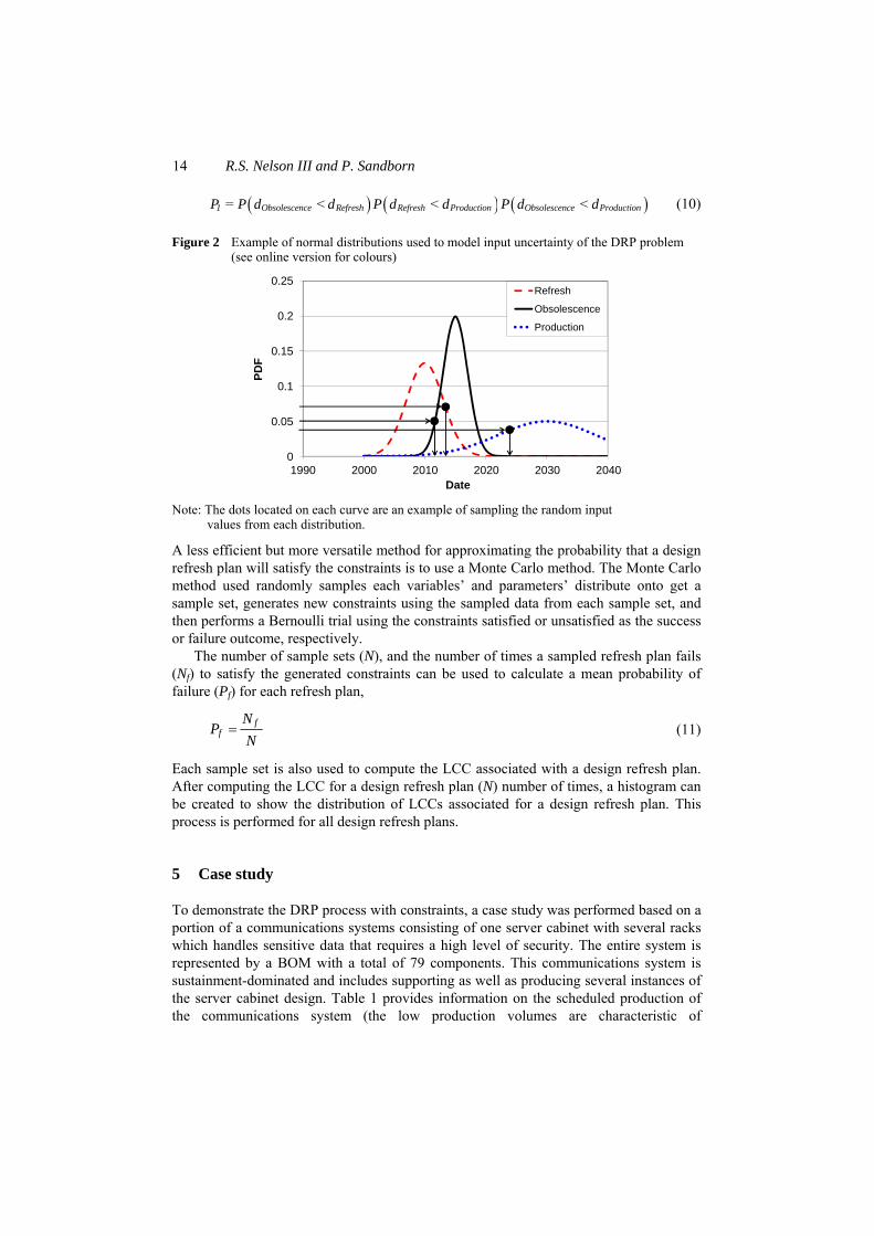
14 R.S. Nelson III and P. Sandborn
( ) ( ) ( )= < < <1 Obsolescence Refresh Refresh Production Obsolescence ProductionP P d d P d d P d d (10)
Figure 2 Example of normal distributions used to model input uncertainty of the DRP problem (see online version for colours)
0
0.05
0.1
0.15
0.2
0.25
1990 2000 2010 2020 2030 2040
Date
Refresh
Obsolescence
Production
Note: The dots located on each curve are an example of sampling the random input values from each distribution.
A less efficient but more versatile method for approximating the probability that a design refresh plan will satisfy the constraints is to use a Monte Carlo method. The Monte Carlo method used randomly samples each variables’ and parameters’ distribute onto get a sample set, generates new constraints using the sampled data from each sample set, and then performs a Bernoulli trial using the constraints satisfied or unsatisfied as the success or failure outcome, respectively.
The number of sample sets (N), and the number of times a sampled refresh plan fails (Nf) to satisfy the generated constraints can be used to calculate a mean probability of failure (Pf) for each refresh plan,
ff
NP
N= (11)
Each sample set is also used to compute the LCC associated with a design refresh plan. After computing the LCC for a design refresh plan (N) number of times, a histogram can be created to show the distribution of LCCs associated for a design refresh plan. This process is performed for all design refresh plans.
5 Case study
To demonstrate the DRP process with constraints, a case study was performed based on a portion of a communications systems consisting of one server cabinet with several racks which handles sensitive data that requires a high level of security. The entire system is represented by a BOM with a total of 79 components. This communications system is sustainment-dominated and includes supporting as well as producing several instances of the server cabinet design. Table 1 provides information on the scheduled production of the communications system (the low production volumes are characteristic of
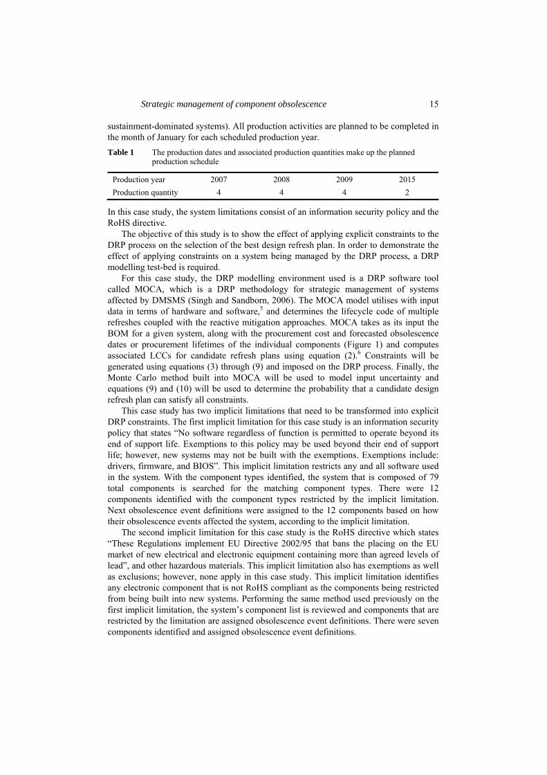
Strategic management of component obsolescence 15
sustainment-dominated systems). All production activities are planned to be completed in the month of January for each scheduled production year. Table 1 The production dates and associated production quantities make up the planned
production schedule
Production year 2007 2008 2009 2015 Production quantity 4 4 4 2
In this case study, the system limitations consist of an information security policy and the RoHS directive.
The objective of this study is to show the effect of applying explicit constraints to the DRP process on the selection of the best design refresh plan. In order to demonstrate the effect of applying constraints on a system being managed by the DRP process, a DRP modelling test-bed is required.
For this case study, the DRP modelling environment used is a DRP software tool called MOCA, which is a DRP methodology for strategic management of systems affected by DMSMS (Singh and Sandborn, 2006). The MOCA model utilises with input data in terms of hardware and software,5 and determines the lifecycle code of multiple refreshes coupled with the reactive mitigation approaches. MOCA takes as its input the BOM for a given system, along with the procurement cost and forecasted obsolescence dates or procurement lifetimes of the individual components (Figure 1) and computes associated LCCs for candidate refresh plans using equation (2).6 Constraints will be generated using equations (3) through (9) and imposed on the DRP process. Finally, the Monte Carlo method built into MOCA will be used to model input uncertainty and equations (9) and (10) will be used to determine the probability that a candidate design refresh plan can satisfy all constraints.
This case study has two implicit limitations that need to be transformed into explicit DRP constraints. The first implicit limitation for this case study is an information security policy that states “No software regardless of function is permitted to operate beyond its end of support life. Exemptions to this policy may be used beyond their end of support life; however, new systems may not be built with the exemptions. Exemptions include: drivers, firmware, and BIOS”. This implicit limitation restricts any and all software used in the system. With the component types identified, the system that is composed of 79 total components is searched for the matching component types. There were 12 components identified with the component types restricted by the implicit limitation. Next obsolescence event definitions were assigned to the 12 components based on how their obsolescence events affected the system, according to the implicit limitation.
The second implicit limitation for this case study is the RoHS directive which states “These Regulations implement EU Directive 2002/95 that bans the placing on the EU market of new electrical and electronic equipment containing more than agreed levels of lead”, and other hazardous materials. This implicit limitation also has exemptions as well as exclusions; however, none apply in this case study. This implicit limitation identifies any electronic component that is not RoHS compliant as the components being restricted from being built into new systems. Performing the same method used previously on the first implicit limitation, the system’s component list is reviewed and components that are restricted by the limitation are assigned obsolescence event definitions. There were seven components identified and assigned obsolescence event definitions.
16 R.S. Nelson III and P. Sandborn
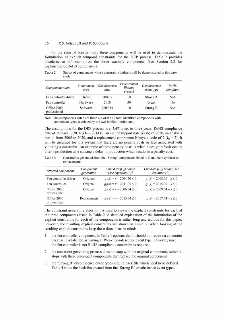
For the sake of brevity, only three components will be used to demonstrate the formulation of explicit temporal constraints for the DRP process. Table 2 provides obsolescence information on the three example components (see Section 2.2 for explanation of RoHS compliance). Table 2 Subset of components whose constraint synthesis will be demonstrated in this case
study
Component name Component type
Obsolescence date
Procurement lifetime (years)
Obsolescence event type
RoHS compliant
Fan controller driver Driver 2007.5 10 Strong A N/A Fan controller Hardware 2018 30 Weak No Office 2000 professional
Software 2009.54 10 Strong B N/A
Note: The components listed are three out of the 19 total identified components with component types restricted by the two implicit limitations.
The assumptions for the DRP process are: LAT is set to three years, RoHS compliance date of January 1, 2014 (DC = 2014.0), an end of support date (EOS) of 2020, an analysis period from 2005 to 2020, and a replacement component lifecycle code of 2 (IR = 2). It will be assumed for this system that there are no penalty costs or fees associated with violating a constraint. An example of these penalty costs is when a design refresh occurs after a production date causing a delay in production which results in a penalty cost. Table 3 Constraints generated from the ‘Strong’ components listed in 2 and their synthesised
replacements
Affected component Component generation
Start date (CS) bound [see equation (5)]
End date (CE) bound [see equation (7)]
Fan controller driver Original g1(x) = x – 2004.50 ≤ 0 g2(x) = 2008.00 – x ≤ 0 Fan controller Original g3(x) = x – 2011.00 ≤ 0 g4(x) = 2015.00 – x ≤ 0 Office 2000 professional
Original g5(x) = x – 2006.54 ≤ 0 g6(x) = 2009.54 – x ≤ 0
Office 2000 professional
Replacement g7(x) = x – 2015.54 ≤ 0 g8(x) = 2017.54 – x ≤ 0
The constraint generating algorithm is used to create the explicit constraints for each of the three components listed in Table 2. A detailed explanation of the formulation of the explicit constraints for each of the components is rather long and tedious for this paper; however, the resulting explicit constraints are shown in Table 3. When looking at the resulting explicit constraints keep these three ideas in mind:
1 the fan controller component in Table 1 appears that it should not require a constraint because it is labelled as having a ‘Weak’ obsolescence event type; however, since the fan controller is not RoHS compliant a constraint is required
2 the constraint generating process does not stop with the original component, rather it stops with there placement components that replace the original component
3 the ‘Strong B’ obsolescence event types require back fits which need to be defined. Table 4 show the back fits created from the ‘Strong B’ obsolescence event types.
Strategic management of component obsolescence 17
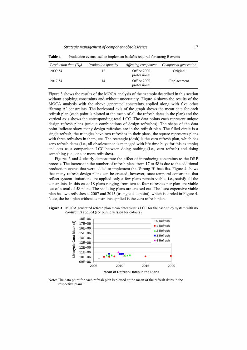
Table 4 Production events used to implement backfits required for strong B events
Production date (DP) Production quantity Affecting component Component generation
2009.54 12 Office 2000 professional
Original
2017.54 14 Office 2000 professional
Replacement
Figure 3 shows the results of the MOCA analysis of the example described in this section without applying constraints and without uncertainty. Figure 4 shows the results of the MOCA analysis with the above generated constraints applied along with five other ‘Strong A’ constraints. The horizontal axis of the graph shows the mean date for each refresh plan (each point is plotted at the mean of all the refresh dates in the plan) and the vertical axis shows the corresponding total LCC. The data points each represent unique design refresh plans (unique combinations of design refreshes). The shape of the data point indicate show many design refreshes are in the refresh plan. The filled circle is a single refresh, the triangles have two refreshes in their plans, the square represents plans with three refreshes in them, etc. The rectangle (dash) is the zero refresh plan, which has zero refresh dates (i.e., all obsolescence is managed with life time buys for this example) and acts as a comparison LCC between doing nothing (i.e., zero refresh) and doing something (i.e., one or more refreshes).
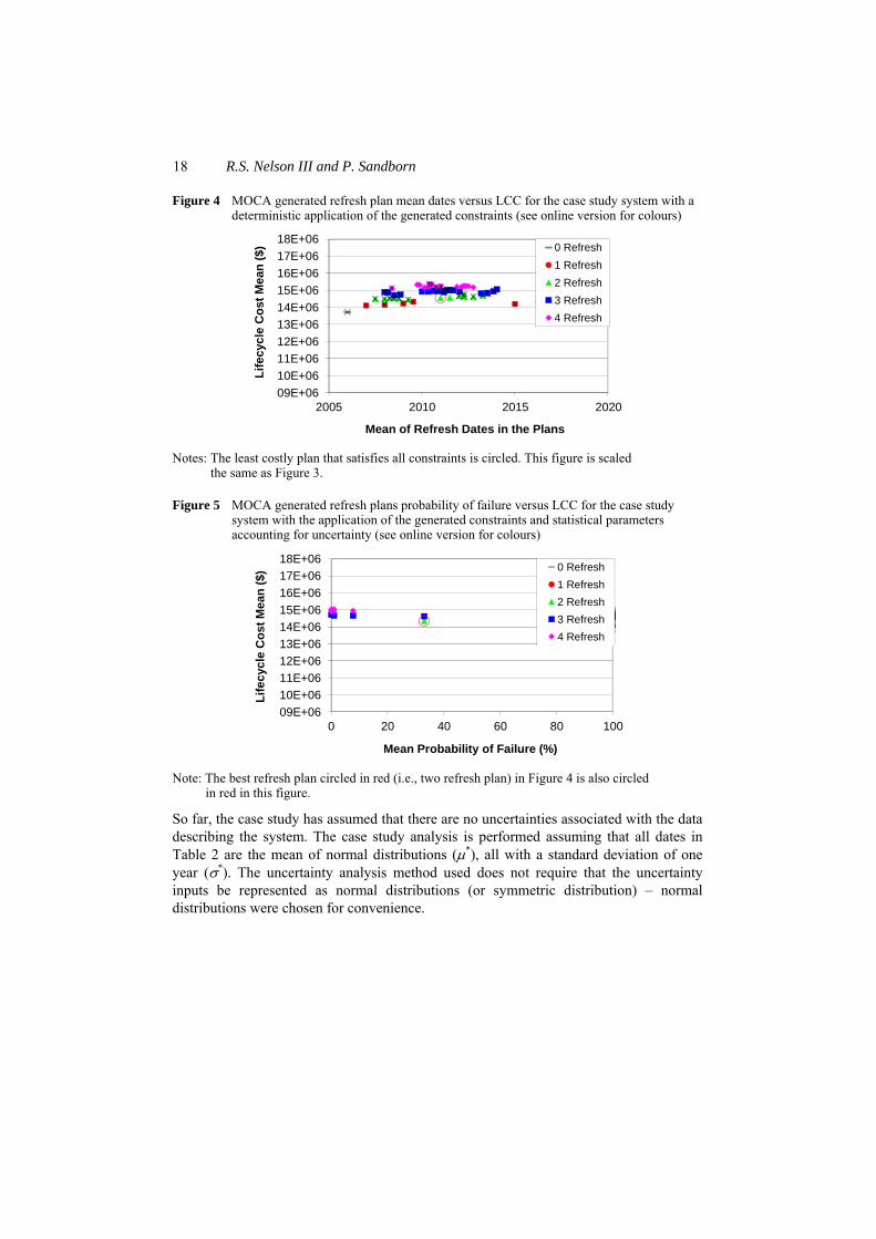
Figures 3 and 4 clearly demonstrate the effect of introducing constraints to the DRP process. The increase in the number of refresh plans from 17 to 58 is due to the additional production events that were added to implement the ‘Strong B’ backfits. Figure 4 shows that many refresh design plans can be created; however, once temporal constraints that reflect system limitations are applied only a few plans remain viable, i.e., satisfy all the constraints. In this case, 18 plans ranging from two to four refreshes per plan are viable out of a total of 58 plans. The violating plans are crossed out. The least expensive viable plan has two refreshes at 2007 and 2015 (triangle data point), which is circled in Figure 4. Note, the best plan without constraints applied is the zero refresh plan.
Figure 3 MOCA generated refresh plan mean dates versus LCC for the case study system with no constraints applied (see online version for colours)
09E+0610E+0611E+0612E+0613E+0614E+0615E+0616E+0617E+0618E+06
2005 2010 2015 2020
Life
cycl
e C
ost M
ean
($)
Mean of Refresh Dates in the Plans
0 Refresh1 Refresh2 Refresh3 Refresh4 Refresh
Note: The data point for each refresh plan is plotted at the mean of the refresh dates in the respective plans.
18 R.S. Nelson III and P. Sandborn
Figure 4 MOCA generated refresh plan mean dates versus LCC for the case study system with a deterministic application of the generated constraints (see online version for colours)
09E+0610E+0611E+0612E+0613E+0614E+0615E+0616E+0617E+0618E+06
2005 2010 2015 2020
Life
cycl
e C
ost M
ean
($)
Mean of Refresh Dates in the Plans
0 Refresh1 Refresh2 Refresh3 Refresh4 Refresh
Notes: The least costly plan that satisfies all constraints is circled. This figure is scaled the same as Figure 3.
Figure 5 MOCA generated refresh plans probability of failure versus LCC for the case study system with the application of the generated constraints and statistical parameters accounting for uncertainty (see online version for colours)
09E+0610E+0611E+0612E+0613E+0614E+0615E+0616E+0617E+0618E+06
0 20 40 60 80 100
Life
cycl
e C
ost M
ean
($)
Mean Probability of Failure (%)
0 Refresh1 Refresh2 Refresh3 Refresh4 Refresh
Note: The best refresh plan circled in red (i.e., two refresh plan) in Figure 4 is also circled in red in this figure.
So far, the case study has assumed that there are no uncertainties associated with the data describing the system. The case study analysis is performed assuming that all dates in Table 2 are the mean of normal distributions (μ*), all with a standard deviation of one year (σ*). The uncertainty analysis method used does not require that the uncertainty inputs be represented as normal distributions (or symmetric distribution) – normal distributions were chosen for convenience.
Strategic management of component obsolescence 19
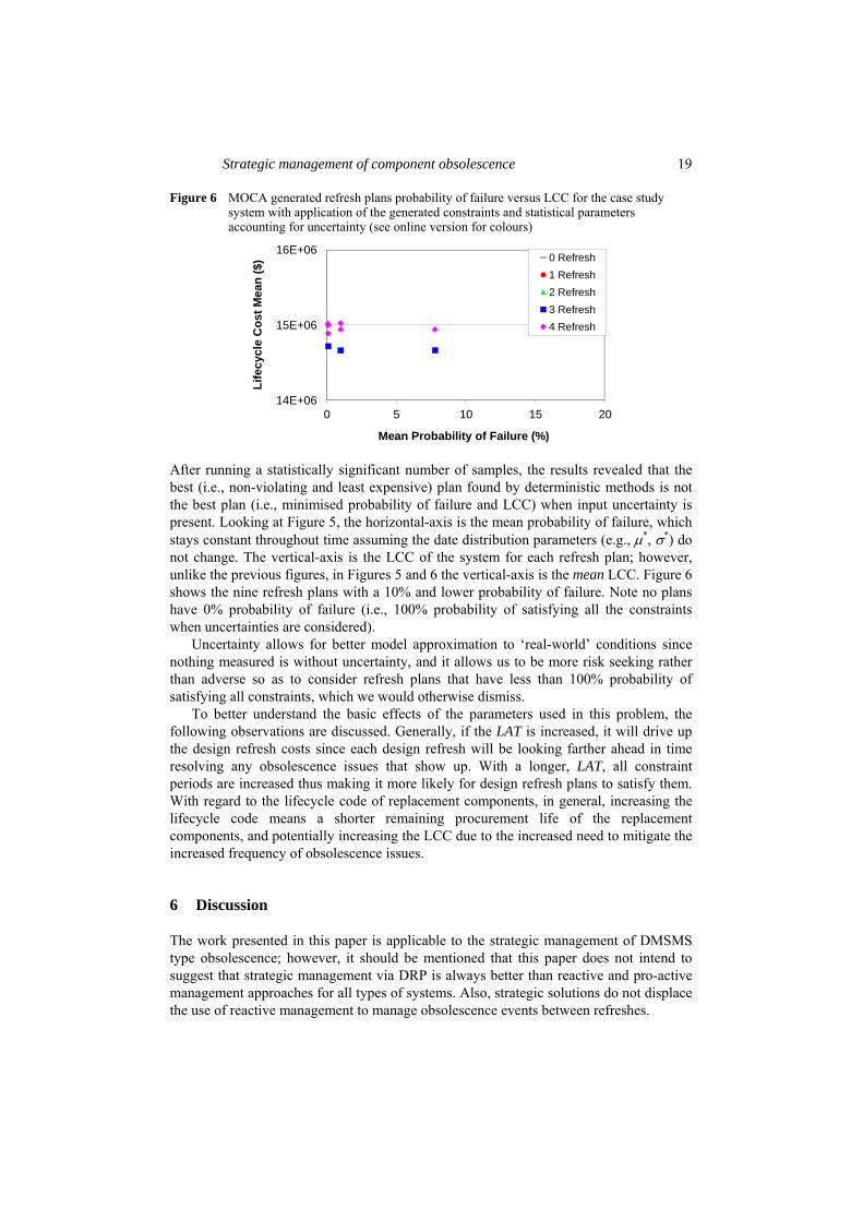
Figure 6 MOCA generated refresh plans probability of failure versus LCC for the case study system with application of the generated constraints and statistical parameters accounting for uncertainty (see online version for colours)
14E+06
15E+06
16E+06
0 5 10 15 20
Life
cycl
e C
ost M
ean
($)
Mean Probability of Failure (%)
0 Refresh1 Refresh2 Refresh3 Refresh4 Refresh
After running a statistically significant number of samples, the results revealed that the best (i.e., non-violating and least expensive) plan found by deterministic methods is not the best plan (i.e., minimised probability of failure and LCC) when input uncertainty is present. Looking at Figure 5, the horizontal-axis is the mean probability of failure, which stays constant throughout time assuming the date distribution parameters (e.g., μ*, σ*) do not change. The vertical-axis is the LCC of the system for each refresh plan; however, unlike the previous figures, in Figures 5 and 6 the vertical-axis is the mean LCC. Figure 6 shows the nine refresh plans with a 10% and lower probability of failure. Note no plans have 0% probability of failure (i.e., 100% probability of satisfying all the constraints when uncertainties are considered).
Uncertainty allows for better model approximation to ‘real-world’ conditions since nothing measured is without uncertainty, and it allows us to be more risk seeking rather than adverse so as to consider refresh plans that have less than 100% probability of satisfying all constraints, which we would otherwise dismiss.
To better understand the basic effects of the parameters used in this problem, the following observations are discussed. Generally, if the LAT is increased, it will drive up the design refresh costs since each design refresh will be looking farther ahead in time resolving any obsolescence issues that show up. With a longer, LAT, all constraint periods are increased thus making it more likely for design refresh plans to satisfy them. With regard to the lifecycle code of replacement components, in general, increasing the lifecycle code means a shorter remaining procurement life of the replacement components, and potentially increasing the LCC due to the increased need to mitigate the increased frequency of obsolescence issues.
6 Discussion
The work presented in this paper is applicable to the strategic management of DMSMS type obsolescence; however, it should be mentioned that this paper does not intend to suggest that strategic management via DRP is always better than reactive and pro-active management approaches for all types of systems. Also, strategic solutions do not displace the use of reactive management to manage obsolescence events between refreshes.
20 R.S. Nelson III and P. Sandborn
The uncertainty modelling presented in this paper assumes that there are no costs associated with the order of events (e.g., design refresh events, obsolescence events, and production events) even when the order of events violates a constraint. To model costs associated with the order of events, two key pieces of information need to be developed:
1 the probability a specific order of events will occur
2 a method for calculating the associated costs for the specific order of events.
The probability that a specific order of events will occur can be found by using a probability aggregate. Determining the cost associated with the order of events will involve both time dependent and independent functions. Since each scenario has associated costs and a probability of occurring, then an expected value could be calculated for each design refresh plan put into the DRP objective function.
The case study demonstrated the effect of imposing temporal constraints not only on the best solution, but on all solutions (Figure 4). For example, imposing the constraints based on ‘Strong B’ obsolescence type events results in all design refresh plans increasing their associated LCC due to the backfit costs needed to implement the design refresh on fielded systems.
While theoretically, a refresh plan can always be found that satisfies all constraints all the time in the presence of uncertainties, in the real world there are several practical limitations on refresh plans and it is common for real systems that the actual set of refresh plans you have to select from will not include any plans that satisfy all the constraints all the time. This happens due to the fact that the plans you have to select from either:
1 conform to a particular management tradition, style, or culture (e.g., the use of a fixed frequency refresh planning scheme)
2 they were generated by an algorithm that conforms to a set of generation rules [e.g., some DRP methodologies use a ‘just in time’ refresh approach, Singh and Sandborn (2006)].
Therefore, it is valuable to be able to choose the best refresh plan from a set of refresh plans where none of the refresh plans satisfy all the criteria all the time. The results of the case study concluded with a graph of the criterion space (Figure 6), which placed emphasis on the question ‘what is the ‘best’ solution?’ Finding the ‘best’ solution could be done by various multi-objective algorithms that include preferences such as a utility function method, which are well developed in optimisation literature. If preferences are not included then the most straight forward method for finding the ‘best’ solution would be to find the design refresh plan with the lowest probability of failure and lowest associated LCC, which is done by normalising both objectives and determining which design refresh plan is closest to the origin.
The refresh plans produced by the DRP methodology is widened in scope by taking real world system limitations and transforming them into constraints that can be directly applied to the DRP process. Future work will be developing the expected LCC value calculation which involves deriving a series of probability aggregates for all possible order of events (i.e., event permutations) and creating penalty cost functions for when the order of events results in a constraint violation or an infeasible situation such as when a design refresh activity completes after the scheduled start of a production event.
Strategic management of component obsolescence 21
Acknowledgements
This work was funded by the National Science Foundation through Grant 0928530, 0928628, 0928837. Any opinions, findings, and conclusions or recommendations presented in the paper are those of the authors and do not necessarily reflect the views of the National Science Foundation. The authors would also like to thank the more than 100 companies and organisations that support research activities at the Center for Advanced Life Cycle Engineering at the University of Maryland annually.
References Cattani, K. and Souza, G. (2003) ‘Good buy? Delaying end-of-life purchases’, European Journal of
Operational Research, Vol. 146, pp.216–228. Directive 2002/95/EC of the European Parliament and of the Council 27 January. Electronic Industries Alliance (1997) Product Lifecycle Data Model (ANSI/EIA-724-97), American
National Standards Institute. Gravier, M. and Swartz, S. (2009) ‘The dark side of innovation: exploring obsolescence and supply
chain evolution for sustainment-dominated systems’, Journal of High Technology Management Research, Vol. 20, pp.87–102.
Henke, A. and Lai, S. (1997) ‘Automated parts obsolescence prediction’. Paper Presented at the Diminishing Manufacturing Sources and Material Shortages Conference, San Antonio, Texas.
Josias, C. and Terpenny, J. (2004) ‘Component obsolescence risk assessment’, Paper presented at the Industrial Engineering Research Conference, Houston, Texas.
Kumar, U. and Saranga, H. (2010) ‘Optimal selection of obsolescence mitigation strategies using a restless bandit model’, European Journal of Operational Research, Vol. 200, pp.170–180.
Lee, S. and Grossmann, I.E. (2000) ‘New algorithms for nonlinear generalized disjunctive programming’, Computers & Chemical Engineering, Vol. 24, Nos. 9/10, pp.2125–2141.
Meixell, M. and Wu, S. (2001) ‘Scenario analysis of demand in a technology market using leading indicators’, IEEE Transactions on Semiconductor Manufacturing, Vol. 14, pp.65–78.
Meyer, A., Pretorius, L. and Pretorius, J.H.C. (2004) ‘A model using an obsolescence mitigation timeline for managing component obsolescence of complex or long life systems’, Paper Presented at the Information Engineering Conference, Singapore.
Nelson, R. III and Sandborn, P. (2010) ‘Managing coupled hardware and software obsolescence using constraint-driven design refresh planning’, Proceedings DMSMS Conference, Las Vegas, NV
Nelson, R. III, Sandborn, P., Terpenny, J.P. and Zheng, L. (2011) ‘Modeling constraints in design refresh planning’, ASME International Design Engineering Conferences & Computers and Information in Engineering Conference, Washington, DC.
Pecht, M. and Tiku, S. (2006) ‘Bogus! Electronic manufacturing and consumers confront a rising tide of counterfeit electronics’, IEEE Spectrum, Vol. 43, pp.37–46.
Porter, G. (1998) ‘An economic method for evaluating electronic component obsolescence solutions’, Boeing Company White Paper.
Rai, R. and Terpenny, J. (2008) ‘Principles for managing technological product obsolescence’, IEEE Transactions on Components and Packaging Technologies, Vol. 31, pp.880–889.
Sandborn, P. (2008) ‘Trapped on technology’s trailing edge’, IEEE Spectrum, Vol. 45, pp.42–45. Sandborn, P. and Myers, J. (2008) ‘Designing engineering systems for sustainment’, in Misra, K.
(Ed.): Handbook of Performability Engineering, Springer, London.
22 R.S. Nelson III and P. Sandborn
Sandborn, P., Mauro, F. and Knox, R. (2007) ‘A data mining based approach to electronic part obsolescence forecasting’, IEEE Transactions on Components and Packaging Technologies, Vol. 30, pp.397–401.
Sandborn, P., Prabhakar, V. and Ahmad, O. (2010) ‘Forecasting technology procurement lifetimes for use in managing DMSMS obsolescence’, Microelectronics Reliability, Vol. 51, pp.392–399.
Singh, P. and Sandborn, P. (2006) ‘Obsolescence driven design refresh planning for sustainment-dominated systems’, The Engineering Economist, Vol. 51, pp.115–139.
Solomon, R., Sandborn, P. and Pecht, M. (2000) ‘Electronic part lifecycle concepts and obsolescence forecasting’, IEEE Transactions on Components and Packaging Technologies, Vol. 23, pp.707–713.
Song, Y. and Lau, H. (2004) ‘A periodic review inventory model with application to the continuous review obsolescence problem’, European Journal of Operations Research, Vol. 159, pp.110–120.
Stogdill, R. (1999) ‘Dealing with obsolete parts’, IEEE Design and Test of Computers, Vol. 16, pp.17–25.
Tomczykowski, W. (2003) ‘A study on component obsolescence mitigation strategies and their impact on R&M’, Paper Presented at the Annual Reliability and Maintainability Symposium, 2003, Tampa, Florida.
Wu, S.D., Aytac, B., Berger, R.T. and Armbruster, C.A. (2006) ‘Managing short lifecycle technology products for Agere systems’, Interfaces, Vol. 36, pp.234–247.
Notes 1 Inventory or sudden obsolescence, which is more prevalent in the operations research
literature, refers to the opposite problem to DMSMS obsolescence. Inventory obsolescence occurs when the product design or system component specifications changes such that the inventories of components are no longer required, e.g., (Song and Lau, 2004). Another type of obsolescence which is different from DMSMS and thus not addressed in this paper is functionality improvement dominated obsolescence, which is when manufacturers cannot maintain market share unless they evolve their products in order to keep up with competition and customer expectations (manufacturers are forced to change their products by the market) (Rai and Terpenny, 2008).
2 DMSMS management is not about forecasting and managing the effects of disruptive technologies that cause the effective obsolescence of whole classes of products; rather it is about the much more common problem of individual components (particularly electronic components) being discontinued by a manufacturer in favour of a newer version of the same component.
3 The BOM input into the DRP process can be a collection of information from various levels and sources within an organisation.
4 Inclusive constraint – requires the design variable value to be within the bounds of the constraint to satisfy the constraint. Alternatively, an exclusive constraint requires the design variable value to be outside the bounds of the constraint to satisfy the constraint.
5 Hardware and software can and do have interdependencies, which drive one another’s obsolescence; however, for this case study it will be assumed that each component is independent or de-coupled from the effects of a dependent component’s obsolescence event (Nelson and Sandborn, 2010).
6 Several obsolescence forecasting methods can be used as input to MOCA (Gravier and Swartz, 2009; Henke and Lai, 1997; Josias and Terpenny, 2004; Meixell and Wu, 2001; Meyer et al., 2004; Solomon et al., 2000; Sandborn et al., 2007; Sandborn et al., 2010; Wu et al., 2006). Obsolescence forecasts for electronic components are also available from several commercial sources.