Stratified experiments reexamined with emphasis on multicenter trials

Controlled Clinical Trials 24 (2003) 167–181

0197-2456/03/$—see front matter © 2003 Elsevier Science Inc. All rights reserved.doi:10.1016

/

S0197-2456(02)00305-7

ARTICLE IN PRESS

Stratified experiments reexamined with emphasis on multicenter trials

Jitendra Ganju, Ph.D.

a,

*, Devan V. Mehrotra, Ph.D.

b

a

Chiron Corporation, Emeryville, California, USA

b

Merck Research Laboratories, Blue Bell, Pennsylvania, USA

Manuscript received January 3, 2002; manuscript accepted September 26, 2002

Abstract

In many stratified experiments the researcher fixes the total sample size but either cannot or doesnot exert control over the sample size per stratum. A classic example is a randomized, two-treatment,multicenter clinical trial—the total sample sizes per treatment group are fixed by design but the sam-ple sizes per center are allowed to vary. Standard analyses of continuous data from such trials fail torecognize the random nature of the stratum sizes. We show that this can lead to biased inference andestimation for both so-called “type II” (unequal weighting of strata) as well as “type III” (equalweighting of strata) analyses. We propose an alternative method of analysis that explicitly accountsfor the randomness of the stratum sizes and illustrate its validity using simulations. A reanalysis ofpublished data from a 29-center clinical trial serves to reinforce the key points. © 2003 Elsevier Sci-ence Inc. All rights reserved.

Keywords:

Interaction; Random stratum sizes; Weighting

Introduction

An example that appeared in Cox [1] will be used to motivate the topic of this paper:

Suppose that in comparing two diets 0, 1 the mean live weight increases are, in kilograms,

Males: treatment 0, 100; treatment 1, 120Females: treatment 0, 90; treatment 1, 80

with small standard errors of order 1 kg. The treatment effect (1 versus 0) is thus 20 kg for malesand

�

10 kg for females and interaction, in fact qualitative interaction is . . . present. . . . An

*

Corresponding author: Dr. J. Ganju, Chiron Corp., 4560 Horton Street, U-140, Emeryville, CA 94608.Tel.:

�

1-510-923-6418; fax:

�

1-510-923-3450.E-mail address: [email protected]

168

J. Ganju, D.V. Mehrotra/Controlled Clinical Trials 24 (2003) 167–181

ARTICLE IN PRESS

application is envisaged in which the same treatment is to be applied to all experimental units,e.g. to all animals regardless of sex. Then an average treatment effect is of some interest inwhich the

weights attached to the different levels of the intrinsic factor are proportions in thetarget population

. In the particular example these might be (1/2, 1/2) regardless of the relativefrequencies of males and females in the data. Note also that if the data frequencies are regardedas estimating unknown population proportions

the standard error of the estimated main effectshould include a contribution from the sampling error in the weights. Note especially . . . theprecise definition of main effects depends in an essential way on having a physically meaningfulsystem of weights.

This formulation is in any case fairly rarely appropriate and there is somedanger of calculating standard errors of

artificial parameters

.

The italics are ours; this article will expand on the italicized comments. When planning astratified experiment, the experimenter, though interested in obtaining a predetermined totalnumber of observations for the experiment, sometimes either cannot or does not exert any in-fluence on the number of observations per stratum. A classic example of such an experimentis a randomized, two-treatment, multicenter clinical trial. The sponsor conducting the trialdetermines the total number of patients that need to be enrolled but does not prespecify inany formal manner the number of patients to be enrolled at any given center (stratum). Pa-tients are enrolled at all centers until the total number of patients from all centers (approxi-mately) equals the predetermined total sample size. In large multicenter studies, centers thatwill enroll more patients than a typical center can often be identified before the trial starts.Indeed, sponsors actively try to recruit high-enrolling centers in order to shorten the time in-terval between the first and last patient enrolled.

Continuous data from multicenter trials are typically analyzed using a fixed-effects linearmodel with terms for treatment, center, and, frequently, treatment-by-center interaction(

T

�

C

). Hereafter, an “interaction model” will mean that

T

�

C

is included in the model. Re-gardless of whether

T

�

C

is included, standard analyses address estimation and inferenceinvolving a population parameter referred to as the “overall true treatment effect.” This pa-rameter, which we shall denote by

�

, is estimated by taking a weighted average of treatmenteffects from each center. Two weighting schemes are commonly used. In the first, each cen-ter gets a weight equal to the reciprocal of the total number of centers, regardless of the num-ber of patients enrolled per center (

equal

weighting approach). In the second, each centergets a weight that is proportional to the number of patients enrolled by that center (

unequal

weighting approach). Opinions on which weighting method to use are largely subjective andhave influenced regulatory guidelines, both in the United States and the European Union.The U.S. Food and Drug Administration favors assigning equal weights to centers (as notedin reference [2]), whereas the International Conference on Harmonisation gives its imprima-tur to both weighting approaches [3]. The topic of attaching equal or unequal weights hasbeen debated well before the multicenter trial came in the limelight.

Fleiss [4], who prefers equal weights when the model includes

T

�

C

, lends support to hispreference by noting that Yates [5] recommends it, although elsewhere Yates [6] prefers un-equal weights. Searle [7] favors neither weighting method, whereas Nelder [8,9] finds thehypothesis defined by equal weights uninteresting. The authors that we discuss henceforthspecifically focus on the randomized multicenter trial.

Throughout this paper we will assume that: (1) two treatments, say A and B, are beingcompared in a randomized, double-blind,

C

-center (

C

�

2) clinical trial; (2) within each cen-


169

ARTICLE IN PRESS

ter, patients are randomized to either A or B in an exact

k

1

:

k

2

ratio, where

k

1

and

k

2

representpositive integers; (3) treatment by stratum interaction may exist; and (4) enrollment is com-petitive (i.e., each of the

C

centers will continue to enroll patients into the trial until the totalprespecified sample size for the entire trial has been achieved). To clarify assumption (4)suppose two therapies for treatment of HIV are being compared and that one of the

C

centersis located in an area where the incidence of HIV infection is relatively high. It is natural toexpect that particular center to enroll more patients than other centers. Accordingly, assump-tion (4) means that instead of imposing an artificial restriction such as enforcing approxi-mately equal enrollment, all study centers will enroll patients at a rate proportional to their“enrollment potential.” In statistical terms, assumption (4) is synonymous with the assump-tion of a multinomial distribution for the observed number of patients across the

C

centers(hereafter referred to as “center sizes”). The assumption of a multinomial distribution is notentirely valid because competing factors, such as competition among institutions to enrollpatients, patient referral patterns, etc., could influence its validity. We make this assumptionexplicitly, whereas the same assumption is implicit in many other analyses, namely, the un-equally weighted analysis discussed later as well as analysis of proportions via risk differ-ence, relative risk, or odds ratio. The multinomial assumption is reasonable under a competi-tive enrollment scenario.

At this stage it is necessary to define the population parameter of interest,

�

. To do so,we must first answer the pivotal question: What exactly is the target population? Thefollowing point is significant. Because center is treated as a fixed-effects factor (as op-posed to random), the target population must be viewed as the collection of all eligiblepatients who could have been enrolled at any of the

C

centers selected for the study. Anyattempt to extrapolate the results to a larger population of centers is an inherent violationof the assumption that center effects are fixed. We are not saying that center effectsought to be fixed, but we are pointing out that doing so restricts the definition of

�

andresulting inference. This is not the place for debating whether center effects ought to befixed or random — suffice it to say that treating center effects as fixed is the dominantpractice.

Let

�

i

denote the true fraction of the target population associated with center

i

(i.e., if theentire target population was enrolled,

�

i

would be the resulting proportion of patients en-rolled at center

i

). Let

�

Ai

and

�

Bi

represent the population means at center

i,

so that represents the true treatment effect at center

i

. The overall true treatment ef-fect can be unambiguously defined as

Standard statistical analyses of multicenter data estimate

�

and test the hypothesis

H

0

:

��

0

.Henceforth, without loss of generality, we will set

�

0

equal to zero. As we will discuss later,problems arise with the standard analyses because, depending on the weighting approachused, the estimate of

�

, is either biased (with the equal weighting approach) or its truevariance is underestimated (with the unequal weighting approach). Thus, in either case, in-ferences can be misleading.

∆i µAi µBi–=

∆ πi∆i . i 1=C∑=

∆̂

170


ARTICLE IN PRESS

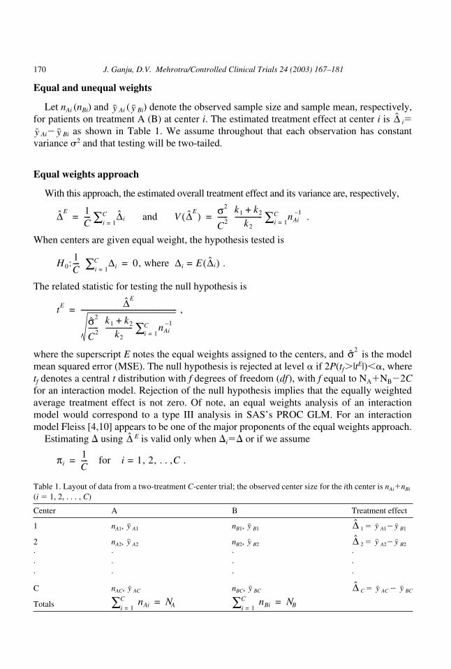
Equal and unequal weights

Let

n

Ai

(

n

Bi

) and

Ai

(

Bi

) denote the observed sample size and sample mean, respectively,for patients on treatment A (B) at center

i

. The estimated treatment effect at center

i

is

i

Ai

�

Bi

as shown in Table 1. We assume throughout that each observation has constantvariance

2

and that testing will be two-tailed.

Equal weights approach

With this approach, the estimated overall treatment effect and its variance are, respectively,

and

When centers are given equal weight, the hypothesis tested is

The related statistic for testing the null hypothesis is

where the superscript

E

notes the equal weights assigned to the centers, and is the modelmean squared error (MSE). The null hypothesis is rejected at level

�

if 2

P

(

t

f

�|tE|) �, wheretf denotes a central t distribution with f degrees of freedom (df), with f equal to NA�NB�2Cfor an interaction model. Rejection of the null hypothesis implies that the equally weightedaverage treatment effect is not zero. Of note, an equal weights analysis of an interactionmodel would correspond to a type III analysis in SAS’s PROC GLM. For an interactionmodel Fleiss [4,10] appears to be one of the major proponents of the equal weights approach.

Estimating � using E is valid only when �i� or if we assume

y y∆̂

y y

∆̂E 1C---- ∆̂i

i 1=C∑= V ∆̂E( ) σ2

C2------

k1 k2+k2

---------------- i 1=C∑ nAi

1– . =

H0:1C----

i 1=C∑ ∆i 0, where ∆i E ∆̂i( ) . ==

tE ∆̂E

σ̂2

C2------

k1 k2+k2

---------------- i 1=C∑ nAi

1–

-------------------------------------------------------- , =

σ̂2

∆̂

πi1C---- for i 1, 2, . . ,C . ==

Table 1. Layout of data from a two-treatment C-center trial; the observed center size for the ith center is nAi�nBi (i 1, 2, . . . , C)

Center A B Treatment effect

1 nA1, A1 nB1, B1 1 A1� B1

2 nA2, A2 nB2, B2 2 A2� B2

· · · ·· · · ·· · · ·

C nAC, AC nBC, BC C AC � BC

Totals

y y ∆̂ y y

y y ∆̂ y y

y y ∆̂ y y

nAi i 1=

C∑ NA= nBi i 1=

C∑ NB=

J. Ganju, D.V. Mehrotra/Controlled Clinical Trials 24 (2003) 167–181 171

ARTICLE IN PRESS

The assumption that

is hard to justify in any trial. It is common knowledge that in the planning of a trial some cen-ters are selected specifically because of their capabilities in recruiting more patients than typ-ical centers, thus annulling the enrollment assumption. In general, E is a biased estimator of�, and the popular type III approach can lead to inaccurate estimation and inference.

Some have suggested that

is the meaningful parameter to estimate even when

because the null hypothesis tests whether

Curiously however, this suggestion (of attaching equal weights) is never extended to binomialoutcomes where the weights attached to the treatment effects at each center are center-specific sample size weights identical to the weights defined in the next section. When inter-action is present, it is important to note that

if (but not if and only if) .

When enrollment is unequal,

does not necessarily imply �0, and conversely �0 does not necessarily imply

Moreover, it is common practice to drop the interaction term if its p-value is “reasonably”large. Under such a scheme the model that includes the interaction term defines the truetreatment effect to be

whereas the model that excludes the interaction term defines the true treatment effect to be�. Clearly, empirical models ought not to define a population parameter.

When the assumption of equal enrollment is not valid, the equally weighted test statistic tE isgenerally biased in favor of rejecting the null hypothesis (see section on simulation results).

πi1C----=

∆̂

1C----

i 1=C∑ ∆i

πi1C---- , ≠

1C----

i 1=C∑ ∆i 0 . =

∆ 1C----

i 1=C∑ ∆i = πi

1C----=

1C----

i 1=C∑ ∆i 0=

1C----

i 1=C∑ ∆i 0 . =

1C----

i 1=C∑ ∆i ,

172 J. Ganju, D.V. Mehrotra/Controlled Clinical Trials 24 (2003) 167–181

ARTICLE IN PRESS

Unequal weights approach

With this approach, the estimated overall treatment effect and its variance are, respectively,

and

where

is the estimate of �i. In light of assumption (2) winAi/NA, and from assumption (4) wi is anunbiased estimate of �i. The superscript U denotes unequal weights assigned to centers.Also, simplifies to A� B, where A( B) represents the observed mean for treatment A(B) unadjusted for centers. (If an exact k1:k2 allocation is not achieved, then

does not simplify to A� B.) Hence the unequal weighting approach assigns unequalweights to centers but equal weights to patients. Centers that enroll more patients are givengreater weight than those enrolling fewer patients. The related statistic for testing the null hy-pothesis H0:�0 is

where, as before, is the model MSE. The null hypothesis is rejected at level � if2P(tf �|tU|) �, with notation as above. Of note, an unequal weights analysis of an interac-tion model would correspond to the use of type II sums of squares in SAS’s PROC GLM.The current view in the literature supports unequal weighting [11–14]. An exception to thecurrent view is Schwemer [15], who prefers equal weights and correctly notes that theweights, wi s, are random variables but that the analysis treats them as constants.

We agree that the center-specific treatment effects should be weighted unequally becausepatients are the experimental units, not centers (or other strata). However, due to randomnessin center sizes, the conventional estimate of V( ) is biased. We show in the appendix thatthe correct expression for V( ) is

(1)

Compare this expression with the conventional but incorrect formula that does not recognize therandomness:

∆̂U wi∆̂i

i 1=C∑= V ∆̂U( )

k1 k2+k2

---------------- σ2

N A

------- , =

wi nAinBi nAi nBi+( ) 1– i 1=C∑ nAinBi nAi nBi+( ) 1–⁄=

∆̂Uy y y y

wi∆̂i i 1=C∑

y y

tU ∆̂U

k1 k2+k2

---------------- σ̂2

N A

-------

------------------------------- , =

σ̂2

∆̂U

∆̂U

1N A

------- k1 k2+

k2---------------- σ2

i 1=C∑ πi ∆i ∆–( )2+ .

k1 k2+k2

---------------- σ2

N A

------- .


ARTICLE IN PRESS

The conventional variance is biased because it underestimates the true variance by

Thus, if there is no interaction, there is no bias. The value of �i that maximizes V( ), orequivalently the bias, is �i1/C. Even though the conventional variance is biased, it is a consis-tent estimator. Larger differences between �i and � lead to larger variances, a fact not recognizedby treating the sample sizes at each center to be fixed. It will come as no surprise to the readerthen when we show later that tU can result in an excessive number of false positives.

A new test statistic

We saw earlier that the equally weighted estimate of the treatment effect is biased and thatthe conventional variance of the unequally weighted estimate is biased. A new test statistic isproposed based on the correct variance for [Eq. (1)], with the unknown population param-eters 2, �i, and �i being replaced with estimated counterparts:

(2)

This new test statistic tests the same hypothesis as the statistic based on unequal weights, tU,namely, H0:�0.

Interestingly, our proposal for analyzing multicenter data has, in effect, a similar flavor to that ofCiminera et al. [16]. In the presence of “substantial” T�C interaction, they argue in favor of usingMS(T�C) as the error term in lieu of MSE. However, their reasoning is unrelated to random sam-ple sizes, and their recommendation applies only when the interaction is qualitative (not all �ishave the same sign), not quantitative (all �is have the same sign). The partial link between theirproposal and ours becomes apparent upon noting that the expression for the expected value ofMS(T�C) is similar in form to our proposed variance in Eq. (1). In other words, when there isT�C interaction (in our case, either quantitative or qualitative), the results based on our proposedstatistic will be similar (but not identical) to that obtained by employing MS(T�C) as the errorterm in the unequally weighted analysis. They also propose a novel way to combine the informa-tion across all the centers. With large sample sizes and variance homogeneity, their weightingscheme can be shown to be equivalent to that used in our proposed statistic.

Results of a simulation study described later show that the new test statistic tN performsreasonably well, while tE and tU do not.

How tN compares with the standard test for a treatmenteffect when center effects are random

We briefly discuss how tN compares with the standard test statistic that tests for a treat-ment effect under a mixed model. The center effects, and hence the T�C effects, are random.

1N A

------- i 1=C∑ πi ∆i ∆–( )2 .

∆̂U

∆̂U

tN ∆̂U

1N A

------- k1 k2+

k2---------------- σ̂ 2

i 1=C∑ π̂i ∆̂i ∆̂U

–( )+

-------------------------------------------------------------------------------------------- . =


ARTICLE IN PRESS

Let us denote the estimated overall treatment effect and test statistic for a treatment effectfrom a mixed model by and tR, respectively. The comparison between tN and tR can beexplained by focusing separately on the point estimate of � and its variance employed byeach test statistic. Jones et al. [17] show that (when allocation is 1:1)

where

In this notation, TC2 denotes the T�C variance component and 2 denotes the residual error

variance (as before). Let

denote the weight attached to the treatment effect from center i. As TC2 →0, �i

, and → (noted by Jones et al.). On the other hand, as TC2 → , �i→ ,

and → E. In general, for 0 2

TC , �i is between

so the mixed model estimate is between E and .

In a mixed model analysis, the mean square for treatment is divided by the mean squarefor T�C, with the latter having an expectation of 2� kTC

2 , where k is �0. Therefore, condi-tional on center sizes, V( ) can be written as

where m is �0. But we have shown that for a fixed-effects model, with 1:1 allocation,

Hence it becomes clear that the denominators of tN and tR have a similar form and are bothgreater than the denominator of tU. Moreover, an increase in the magnitude of the T�C inter-action, that is an increase in 2

TC or

results in an increase in V( ) and V ( ). In summary, the denominators of tN and tR aregreater than the denominator for tU when T�C is included; thus, formulas for tN and tR de-pend on the interaction, whereas the formula for tU does not.

∆̂R

∆̂R V i1– ∆̂ i∑

V i1–∑

-------------------- , = V i σ̂ TC2 σ̂2

n Ai

------- . +=

θi

V i1–

V i1–∑

---------------=

n Ai

N A

------- ∆̂R ∆̂U ∞ 1C----

∆̂R ∆̂ ∞

n Ai

N A

------- and 1C---- ,

∆̂ ∆̂U

∆̂R

2N A

-------σ2 1N A

-------mσ TC2 , +

V ∆̂U( ) 2N A

-------σ2 1N A

------- i 1=C∑ πi ∆i ∆–( )2 . +=

i 1=

C∑ πi ∆i ∆–( )2 ,

∆̂U ∆̂R


ARTICLE IN PRESS

Simulation results

We conducted a simulation study with two objectives: (1) to demonstrate that tN has a nulldistribution that can be approximated by the central t distribution with NA�NB�2C df, and(2) to demonstrate the poor performance of tE and tU. We addressed these objectives by sim-ulating data from hypothetical multicenter trials and computing the percent of times the 95%confidence interval (CI) captured �. The formulas used to construct the CIs were:

The number of centers in our simulated scenarios were either two (“trial 1,” 20 to 40 sub-jects per treatment), six (“trial 2,” 60 to 120 subjects per treatment), or ten (“trial 3,” 100 to200 subjects per treatment). The performance of the three test statistics, tE, tU, and tN, was ex-amined under a 1:1 randomization, with both equal and unequal enrollment. Conditional onthe sample size per treatment, the center sample sizes were generated from a multinomialdistribution with �is as shown in Table 2. The response variable to be analyzed was gener-

∆̂ t .025, N A NB 2–+ C V̂ ∆̂( ) , where

for tE, ∆̂ ∆̂E= and V̂ ∆̂( ) 2=

σ̂2

C2------

i 1=

C∑ n 1–Ai ;

for tU , ∆̂ ∆̂U and V̂ ∆̂( ) 2=

σ̂2

N A

------- ; and

for tN , ∆̂ ∆̂U and V̂ ∆̂( ) 1

N A

-------= 2σ̂2 i 1=

C∑ π̂i ∆̂i ∆̂U–( )

2+ . =

=

±

Table 2. Treatment effects and enrollment rates for three trials

Case 1 Case 2 Case 3

Trial Center �i �i �i �i �i �i

1 1 0.7 0.5 1.00 0.55 1.00 0.62 �0.7 0.5 �11/9 0.45 0.30 0.4

2 1 0.4 1/6 0.4 0.2 1 0.32 0.4 1/6 0.1 0.2 0.2 0.13 0.4 1/6 0.5 0.2 0.5 0.14 �0.4 1/6 �0.5 0.2 0.4 0.15 �0.4 1/6 �0.2 0.1 0.2 0.16 �0.4 1/6 �0.8 0.1 0.1 0.3

3 1 0.3 0.1 0.6 0.08 1.00 0.062 0.3 0.1 0.9 0.08 0.20 0.083 0.3 0.1 0.4 0.09 �0.1 0.084 0.3 0.1 0.7 0.09 0.4 0.095 0.3 0.1 0.47 0.06 0 0.096 �0.3 0.1 �0.4 0.12 0.10 0.117 �0.3 0.1 �0.6 0.12 0 0.118 �0.3 0.1 �0.5 0.11 0.6 0.129 �0.3 0.1 �0.4 0.11 �0.1 0.12

10 �0.3 0.1 �0.2 0.14 0.1 0.14

For cases 1 and 2, � 0 for all three trials. For case 3, � 0.72, 0.46, and 0.189 for trials 1, 2, and 3, respectively.


ARTICLE IN PRESS

ated from a normal distribution with variance for each observation equal to 1. The true stratum-specific treatment effects (�is) for each of the three trials are also shown in Table 2.

Table 2 presents three cases that were examined for each trial. In case 1 there was equalenrollment, interaction, and no overall treatment effect (�0). In case 2 there was unequal enroll-ment, interaction, and no overall treatment effect (�0). In case 3 there was unequal enrollment,interaction, and nonzero treatment effect . Note that for trial 1 under case 3 when thetotal sample size per treatment is 20, the average number of patients at centers 1 and 2 are 12and 8, respectively, the overall treatment effect �0.72, and so on.

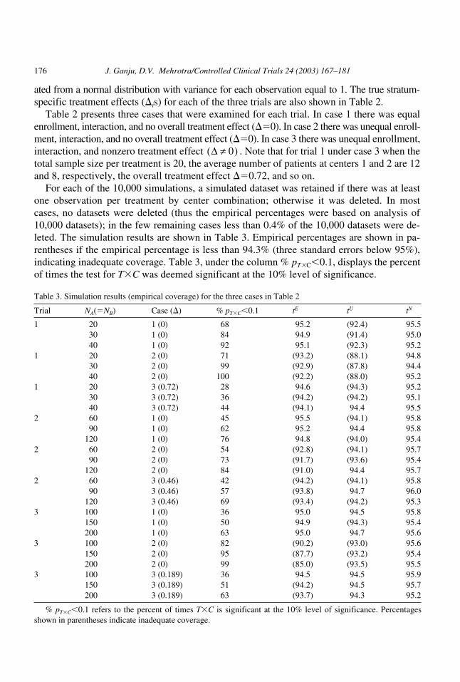
For each of the 10,000 simulations, a simulated dataset was retained if there was at leastone observation per treatment by center combination; otherwise it was deleted. In mostcases, no datasets were deleted (thus the empirical percentages were based on analysis of10,000 datasets); in the few remaining cases less than 0.4% of the 10,000 datasets were de-leted. The simulation results are shown in Table 3. Empirical percentages are shown in pa-rentheses if the empirical percentage is less than 94.3% (three standard errors below 95%),indicating inadequate coverage. Table 3, under the column % pT�C 0.1, displays the percentof times the test for T�C was deemed significant at the 10% level of significance.

∆ 0≠( )

Table 3. Simulation results (empirical coverage) for the three cases in Table 2

Trial NA(NB) Case (�) % pT�C 0.1 tE tU tN

1 20 1 (0) 68 95.2 (92.4) 95.530 1 (0) 84 94.9 (91.4) 95.040 1 (0) 92 95.1 (92.3) 95.2

1 20 2 (0) 71 (93.2) (88.1) 94.830 2 (0) 99 (92.9) (87.8) 94.440 2 (0) 100 (92.2) (88.0) 95.2

1 20 3 (0.72) 28 94.6 (94.3) 95.230 3 (0.72) 36 (94.2) (94.2) 95.140 3 (0.72) 44 (94.1) 94.4 95.5

2 60 1 (0) 45 95.5 (94.1) 95.890 1 (0) 62 95.2 94.4 95.8

120 1 (0) 76 94.8 (94.0) 95.42 60 2 (0) 54 (92.8) (94.1) 95.7

90 2 (0) 73 (91.7) (93.6) 95.4120 2 (0) 84 (91.0) 94.4 95.7

2 60 3 (0.46) 42 (94.2) (94.1) 95.890 3 (0.46) 57 (93.8) 94.7 96.0

120 3 (0.46) 69 (93.4) (94.2) 95.33 100 1 (0) 36 95.0 94.5 95.8

150 1 (0) 50 94.9 (94.3) 95.4200 1 (0) 63 95.0 94.7 95.6

3 100 2 (0) 82 (90.2) (93.0) 95.6150 2 (0) 95 (87.7) (93.2) 95.4200 2 (0) 99 (85.0) (93.5) 95.5

3 100 3 (0.189) 36 94.5 94.5 95.9150 3 (0.189) 51 (94.2) 94.5 95.7200 3 (0.189) 63 (93.7) 94.3 95.2

% pT�C 0.1 refers to the percent of times T�C is significant at the 10% level of significance. Percentagesshown in parentheses indicate inadequate coverage.


ARTICLE IN PRESS

How did tE perform? When there was equal enrollment on average, that is when

tE performed well, as would be expected. However, when enrollment on average was un-equal across centers, then tE yielded biased results. For example, for trial 2, case 2, whenNA60, the empirical coverage of � was 92.8%, significantly smaller than the nominal valueof 95%. As the sample size increased, so did the bias of tE, because

not �.

How did tU perform? tU also performed poorly regardless of whether average enrollmentwas equal or unequal. However, as expected, the performance was dictated by the degree oftreatment by center interaction. We highlight two results. For trial 1, case 2, when NA20, 30,or 40, the empirical coverage of � was well below 90%, the bias being greater with tU thantE. This may be explained by the fact that %pT �C 0.1 was very high and that as

increased, so did the bias of tU. For trial 1, case 3, when NA20 the power to detect interac-tion is low (28%) but tU still results in inadequate coverages.

As mentioned earlier, V( ) is a biased but consistent estimator, so as the sample size in-creases, the bias of tU decreases. This trend in the decrease in bias may not be readily appar-ent in Table 3 because of the variability in the simulated results, but is clear from the formulafor V( ).

How did tN perform? tN performed well, erring on the side of being slightly conservative.For all trials, cases, and sample sizes examined (27 scenarios in all), the empirical coverageranged from 94.4% to 96%.

Reanalysis of multicenter trial data

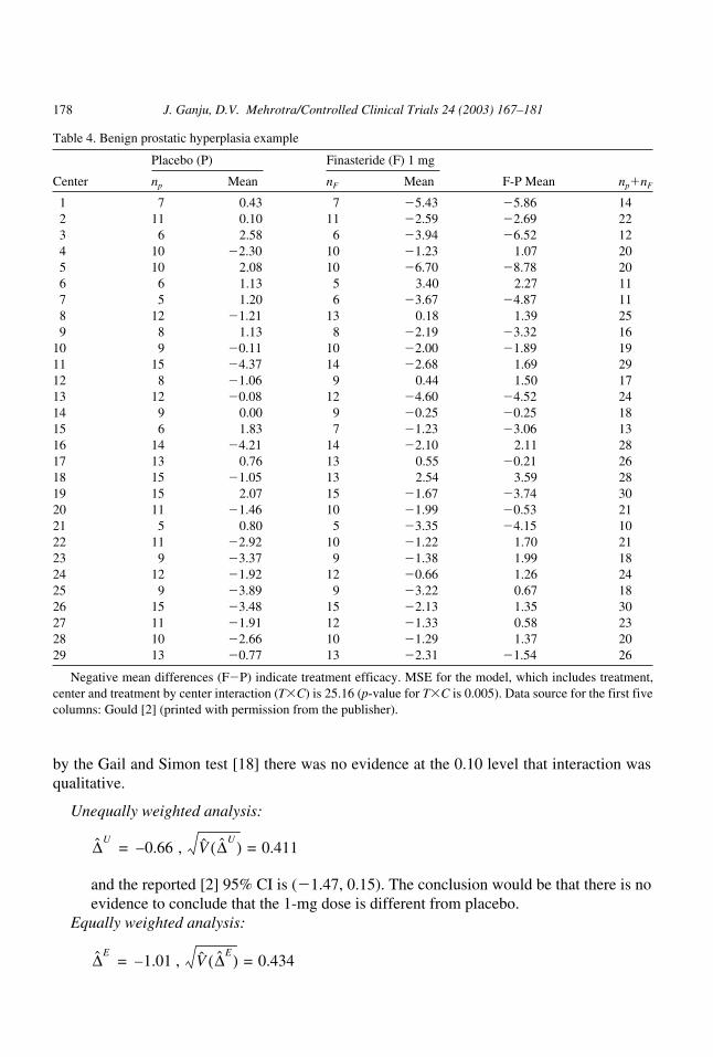
The data from a multicenter trial that will be discussed and reanalyzed in this section wasrecently discussed [2]. The data are shown in Table 4. This was a randomized placebo-con-trolled trial conducted to determine whether the drug, finasteride (F), improved the symp-toms associated with benign prostatic hyperplasia (BPH). BPH, a nonmalignant growth ofthe prostate gland common in aging men, is associated with weak urine flow. Although pa-tients were randomized to receive placebo, 1-mg F, or 5-mg F, discussion here will be lim-ited to comparisons between the placebo and 1-mg F groups. The treatment effects (F meanminus placebo mean) and sample sizes per center are abstracted from the article. Two hun-dred ninety-seven patients were randomized to each treatment arm. Balance was maintainedin most of the 29 centers in that the numbers of patients assigned to placebo or 1-mg F werethe same for most centers. The p-value for T�C was highly significant (p0.005), although

πi1C---- , =

∆̂E 1C----

i 1=

C∑ ∆i , →

i 1=

C∑ ∆i ∆–( )2

∆̂U

∆̂U


ARTICLE IN PRESS

by the Gail and Simon test [18] there was no evidence at the 0.10 level that interaction wasqualitative.

Unequally weighted analysis:

and the reported [2] 95% CI is (�1.47, 0.15). The conclusion would be that there is noevidence to conclude that the 1-mg dose is different from placebo.

Equally weighted analysis:

∆̂U0.66– , V̂ ∆̂U( ) 0.411==

∆̂E1.01 , – V̂ ∆̂E( ) 0.434 ==

Table 4. Benign prostatic hyperplasia example

Placebo (P) Finasteride (F) 1 mg

Center np Mean nF Mean F-P Mean np�nF

1 7 0.43 7 �5.43 �5.86 142 11 0.10 11 �2.59 �2.69 223 6 2.58 6 �3.94 �6.52 124 10 �2.30 10 �1.23 1.07 205 10 2.08 10 �6.70 �8.78 206 6 1.13 5 3.40 2.27 117 5 1.20 6 �3.67 �4.87 118 12 �1.21 13 0.18 1.39 259 8 1.13 8 �2.19 �3.32 16

10 9 �0.11 10 �2.00 �1.89 1911 15 �4.37 14 �2.68 1.69 2912 8 �1.06 9 0.44 1.50 1713 12 �0.08 12 �4.60 �4.52 2414 9 0.00 9 �0.25 �0.25 1815 6 1.83 7 �1.23 �3.06 1316 14 �4.21 14 �2.10 2.11 2817 13 0.76 13 0.55 �0.21 2618 15 �1.05 13 2.54 3.59 2819 15 2.07 15 �1.67 �3.74 3020 11 �1.46 10 �1.99 �0.53 2121 5 0.80 5 �3.35 �4.15 1022 11 �2.92 10 �1.22 1.70 2123 9 �3.37 9 �1.38 1.99 1824 12 �1.92 12 �0.66 1.26 2425 9 �3.89 9 �3.22 0.67 1826 15 �3.48 15 �2.13 1.35 3027 11 �1.91 12 �1.33 0.58 2328 10 �2.66 10 �1.29 1.37 2029 13 �0.77 13 �2.31 �1.54 26

Negative mean differences (F�P) indicate treatment efficacy. MSE for the model, which includes treatment,center and treatment by center interaction (T�C) is 25.16 (p-value for T�C is 0.005). Data source for the first fivecolumns: Gould [2] (printed with permission from the publisher).


ARTICLE IN PRESS

and the 95% CI is (�1.86, �0.16). The conclusion would be that there is evidence toconclude that the 1-mg dose is different from placebo.

The two traditional methods point in opposite directions regarding treatment efficacy. If, as isusually the case, the assumption of equal enrollment is untrue, then conclusions based on tE are notvalid. As is shown next, the conclusion reached with tU is arguably more credible than with tE.

The unequally weighted estimate of the overall true treatment effect (F�placebo) is �0.66and the interaction model MSE is 25.16. The conventional (but biased) estimate of

The correct estimate of

obtained by substituting estimates in Eq. (1), is

Thus, the correct standard error is 8.8% larger than the biased estimate of

The 95% CI based on tN is (�1.85, 0.53); the conclusion is in agreement with that reported [2].

Conclusion

This article is premised on the observation that stratum sizes in many planned experimentsare random and that inferences drawn from traditional analyses can be incorrect since theytreat stratum sizes as fixed. The presentation in this article emphasized randomness in centersizes in multicenter trials. However, in multicenter trials there are other kinds of strata forwhich stratum sizes are allowed to vary, such as gender, age categorized, and baseline dis-ease severity. If the linear model includes interactions between treatment and such strata, it isnecessary to recognize the problems caused by treating the stratum sizes as fixed quantities.

Further research on this topic is needed. For example, the impact of random center sizeswhen the response variable is time to an event in an interaction model analyzed with a Coxregression model deserves to be examined. Other analytic methods for which the potentialadverse impact needs to be examined include the linear mixed-effects model for continuousdata and stratified tests for binary data (e.g., the Mantel-Haenszel test).

Acknowledgments

The bulk of this work was done when the first author was employed by Roche Pharmaceu-ticals. He thanks Dr. Michael Crager for his many insightful remarks. Both authors thank thereferees for their thoughtful comments that led to an improved manuscript.

V ∆̂U( ) is 2 25.16 297⁄× or 0.411.

V ∆̂U( ) ,

0.169 0.031+ or 0.447.

V ∆̂U( ) .


ARTICLE IN PRESS

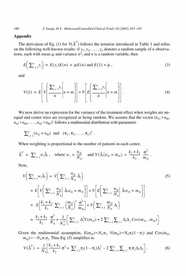
Appendix

The derivation of Eq. (1) for V( ) follows the notation introduced in Table 1 and relieson the following well-known results: if y1, y2, . . . , yn denotes a random sample of n observa-tions, each with mean � and variance 2, and n is a random variable, then

(3)

and

. (4)

We now derive an expression for the variance of the treatment effect when weights are un-equal and center sizes are recognized as being random. We assume that the vector (nA1�nB1,nA2�nB2, . . . , nAC�nBC)� follows a multinomial distribution with parameters

When weighting is proportional to the number of patients in each center,

where and

Now,

(5)

Given the multinomial assumption, E(mAi)NA�i, V(mAi)NA�i(1��i) and Cov(mAi,mAj)�NA�i�j. Thus Eq. (5) simplifies to

(6)

∆̂U

E i 1=

n∑ yi E yi( )E n( ) µE n( ) and E y( ) µ , == =

V y( ) E V

i 1=

n∑ yi

n------------------ n m=

V E

i 1=

n∑ yi

n------------------ n m=

+=

i 1=

C∑ nAi nBi+( ) and π1, π2, . . ., πC( )′ .

∆̂U

i 1=

n∑ wi∆̂i , = wi

nAi

N A

------- = V ∆̂i nAi mAi=( )k1 k2+

k2----------------

σ2

mAi

------- . =

V i 1=C∑ wi∆̂i

V i 1=C∑

nAi

N A

------- ∆̂i

E V i 1=C∑ nAi

N A

------- ∆̂inAi mAi=

V E i 1=C∑ nAi

N A

------- ∆̂inAi mAi=

Ek1 k2+

k2----------------

i 1=C∑

mAi

N A

-------

2

σ2

mAi

------- V i 1=C∑

mAi

N A

------- ∆i

k1 k2+

k2----------------

σ2

N A

------- 1

N A2

--------- i 1=C∑ ∆i

2V mAi( ) 2 i 1=C∑

j i<∑ ∆i∆ j Cov mAi , mAj( )+ .+=

+=

+

=

=

V ∆̂U( ) 1N A

-------k1 k2+

k2---------------- σ2

i 1=C∑ πi 1 πi–( )∆i

2 2 i 1=C∑

j i<∑ πiπ j∆i∆ j–+ . =


ARTICLE IN PRESS

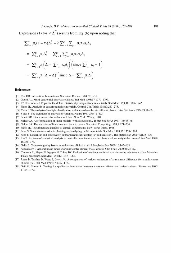
Expression (1) for V( ) results from Eq. (6) upon noting that

References

[1] Cox DR. Interaction. International Statistical Review 1984;52:1–31.[2] Gould AL. Multi-centre trial analysis revisited. Stat Med 1998;17:1779–1797.[3] ICH Harmonised Tripartite Guideline. Statistical principles for clinical trials. Stat Med 1999;18:1905–1942.[4] Fleiss JL. Analysis of data from multiclinic trials. Control Clin Trials 1986;7:267–275.[5] Yates F. The analysis of multiple classification with unequal numbers in different classes. J Am Stat Assoc 1934;29:51–66.[6] Yates F. The technique of analysis of variance. Nature 1947;27:472–473.[7] Searle SR. Linear models for unbalanced data. New York: Wiley, 1987.[8] Nelder JA. A reformulation of linear models (with discussion). J R Stat Soc Ser A 1977;140:48–76.[9] Nelder JA. The statistics of linear models: back to basics. Statistical Computing 1994;4:221–234.

[10] Fleiss JL. The design and analysis of clinical experiments. New York: Wiley, 1986.[11] Senn S. Some controversies in planning and analysing multicentre trials. Stat Med 1998;17:1753–1765.[12] Senn S. Consensus and controversy in pharmaceutical statistics (with discussion). The Statistician 2000;49:135–176.[13] Lin Z. An issue of statistical analysis in controlled multicentre studies: how shall we weight the centres? Stat Med 1999;

18:365–373.[14] Gallo P. Center-weighting issues in multicenter clinical trials. J Biopharm Stat 2000;10:145–163.[15] Schwemer G. General linear models for multicenter clinical trials. Control Clin Trials 2000;21:21–29.[16] Ciminera JL, Heyse JF, Nguyen H, Tukey JW. Evaluation of multicentre clinical trial data using adaptations of the Mosteller-

Tukey procedure. Stat Med 1993;12:1047–1061.[17] Jones B, Teather D, Wang J, Lewis JA. A comparison of various estimators of a treatment difference for a multi-centre

clinical trial. Stat Med 1998;17:1767–1777.[18] Gail M, Simon R. Testing for qualitative interaction between treatment effects and patient subsets. Biometrics 1985;

41:361–372.

∆̂U

i 1=C∑ πi 1 πi–( )∆i

2 2 i 1=C∑

j i<∑ πiπ j∆i∆ j

–

i 1=C∑ πi∆i

2 i 1=C∑

j 1=C∑ πiπ j∆i∆ j

–

i 1=C∑ πi ∆i

i 1=C∑ πi∆i–

2

since i 1=C∑ πi 1=

i 1=C∑ πi ∆i ∆–( )2 since ∆

i 1=C∑ πi∆i=

.

=

=

=

Documents

Stratified experiments reexamined with emphasis on multicenter trials