Embed Size (px)
Citation preview
Noname manuscript No.(will be inserted by the editor)
Stream Engines Meet Wireless Sensor Networks:Cost-Based Planning and Processing of Complex Queriesin AnduIN
Daniel Klan1 · Marcel Karnstedt3 · Katja Hose2 · Liz Ribe-Baumann1 ·Kai-Uwe Sattler1
Received: date / Accepted: date
Abstract Wireless sensor networks are powerful, dis-
tributed, self-organizing systems used for event and en-
vironmental monitoring. In-network query processors
like TinyDB afford a user friendly SQL-like applica-
tion development. Due to sensor nodes’ resource limi-
tations, monolithic approaches often support only a re-
stricted number of operators. For this reason, complex
processing is typically outsourced to the base station
as a part of processing tasks. Nevertheless, previous
work has shown that complete or partial in-network
processing can be more efficient than the base station
approach. In this paper, we introduce AnduIN , a sys-
tem for developing, deploying, and running complex in-
network processing tasks. Particularly, we present the
query planning and execution strategies used in An-
duIN , which combines sensor-local in-network process-
ing and a data stream engine. Query planning em-
ploys a multi-dimensional cost model taking energy
consumption into account and decides autonomously
which query parts will be processed within the sensor
network and which parts will be processed at the cen-
tral instance.
Keywords sensor networks · data streams · power
awareness · distributed computation · in-network query
processing · query planning
This work was in parts supported by the BMBF under grant03WKBD2B and by the Science Foundation Ireland under Grant
No. SFI/08/CE/I1380 (Lion-2) and 08/SRC/I1407 (Clique).
1 Databases and Information Systems Group, Ilmenau Universityof Technology, Germany2 Max-Planck-Institut fur Informatik, Saarbrucken, Germany3 DERI, NUI Galway, Ireland
1 Introduction
In recent years, work to bridge the gap between the
real world and IT systems has opened numerous appli-
cations and has become a major challenge. Sensors for
measuring different kinds of phenomena are an impor-
tant building block in the realization of this vision. To-
day’s increasing miniaturization of mobile devices and
sensor technologies facilitates the construction and de-
velopment of Wireless Sensor Networks (WSN). WSN
are (usually self-organized) networks of sensor nodes
that are equipped with a small CPU, memory, radio
for wireless communication as well as sensing capabili-
ties, e.g., for measuring temperature, light, pressure, or
carbon dioxide. WSN are usually deployed in situations
where large areas have to be monitored or where the
environment prohibits the installation of wired sensing
devices.
However, WSN are typically characterized by rather
limited resources in terms of CPU power, memory size
and – due to their battery-powered operation – limited
lifetime. In fact, the most expensive operation on sen-
sor nodes is wireless communication, and thus, power
efficient operation is one of the major challenges in the
development of both WSN devices and applications. Ta-
ble 1 shows some measurements from a real node, which
was equipped with an ARM LPC2387 CPU, CC110
transceiver, 512 KB flash and 98KB RAM, running a
Contiki-based OS.
In order to reduce energy consumption and to in-
crease the lifetime of the sensors, several approaches
have been developed in recent years. In addition to the
utilization of nodes’ sleep modes through the synchro-
nization of their sampling rates (e.g., in the SMACS
protocol [47]) and the use of special routing protocols
such as LEACH [41], sensor-local (pre-)processing of
2
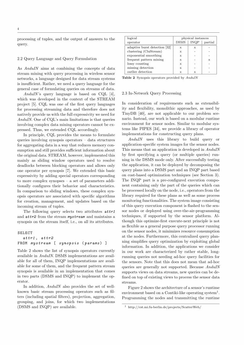
operator energy in µJ
measuring humidity 1655.3
outlier detection (distance based approach,standard deviation, window size 10) 110.7
sending up to 62Byte (see section 3.2.3) 7344.8
Table 1 Measured energy consumption on a sensor node
data is one of the most promising approaches to reduc-
ing energy consumption. However, because the storage
capacity of sensor nodes is limited and the (possibly
aggregated) data is often needed by applications run-
ning outside of the WSN, local processing covers only a
portion of the sensor data processing pipeline. Thus,
the second challenge for a development and process
paradigm is the development of power-aware WSN ap-
plications.
Basically, we can distinguish between three query-
oriented approaches:
– In the store & process model (SPM), the data mea-
sured at the sensor nodes is stored in a database
(which could be a central database or even local
databases at the sensor nodes) and processed after-
wards with a classic database approach by formu-
lating queries.
– In the data stream model (DSM), the WSN is con-
sidered a source for continuous streams of measure-
ments. These streams are processed online by a data
stream management system.
– In the in-network query processing model (INQP),
the processing capacity of the sensor nodes is ex-
ploited by pushing portions of the query plan to the
nodes. These processing steps can comprise prepro-
cessing (filtering), aggregation, or even more com-
plex analytical functions like data mining.
In most applications, a mix of two or even all of these
models is needed. As a typical use case, consider en-
vironment monitoring and particularly water monitor-
ing in marine-based research or wastewater monitoring.
Here, monitoring buoys, flow gauges, and wave moni-
toring instrumentation are deployed in open water, bay
areas, or rivers. These buoys are equipped with sen-
sor for temperature, salinity, oxygen, water quality, or
wave and tide. Obviously, these sensors cannot be used
for wired power and data transmission and are only
deployable as wireless sensor nodes. Furthermore, the
sensor data can be partially processed locally (e.g., pre-
aggregation and cleaning of data), but has to be trans-
mitted to a central unit for further analysis.
This example raises two central questions:
(1) How is an appropriate processing pipeline designed
– ideally in a declarative way (e.g., as a query)?
(2) How can the pipeline be partitioned among the
different models – i.e., which steps should be per-
formed inside the network, which outside the WSN
in an online manner, and which data should be
stored permanently and processed offline?
This latter decision in particular is driven by processing
costs and – more importantly – energy consumption.
Based on these observations, we present in this pa-
per our system AnduIN , which addresses these chal-
lenges by providing a combination of data stream pro-
cessing and in-network query processing. AnduIN sup-
ports CQL as a declarative query interface as well as
a graphical box-and-arrow interface [33]. In addition to
standard CQL operators, it offers several advanced an-
alytical operators for data streams in the form of syn-
opses operators, including burst and outlier detection,
frequent pattern mining, and clustering. AnduIN sup-
ports distributed query processing by pushing portions
of the query plan to the sensor nodes in order to imple-
ment the INQP paradigm. The decision on query de-
composition (whether the plan should be decomposed
and which part should be pushed to the sensor nodes)
is taken by AnduIN ’s query planner. The main contri-
butions of this paper are twofold:
– We propose a hybrid processing model of INQP and
DSM that facilitates the formulation of sensor data
processing as declarative queries and includes ad-
vanced data preparation and analytics operators.
– We discuss a cost model for distributed queries that
takes energy consumption of query operators as an
additional cost dimension into account. Further-
more, we present a query planning and optimization
strategy for deriving the optimal plan decomposi-
tion with respect to the estimated costs.
The remainder of the paper is structured as follows.
After introducing the overall architecture of AnduIN
in Section 2, we present in Section 3 our query plan-
ning approach comprising an optimization strategy and
the cost model taking energy consumption into account.
Results of an experimental evaluation showing the ef-
fectivity of the planning approach are discussed in Sec-
tion 4. Finally, after a discussion of related work in Sec-
tion 5, we conclude the paper by pointing out to future
work.
2 Architecture
AnduIN aims at optimizing query processing for wire-
less sensor networks by considering the benefits of both
in-network query processing (INQP) and the use of
a data stream management system (DSMS) running
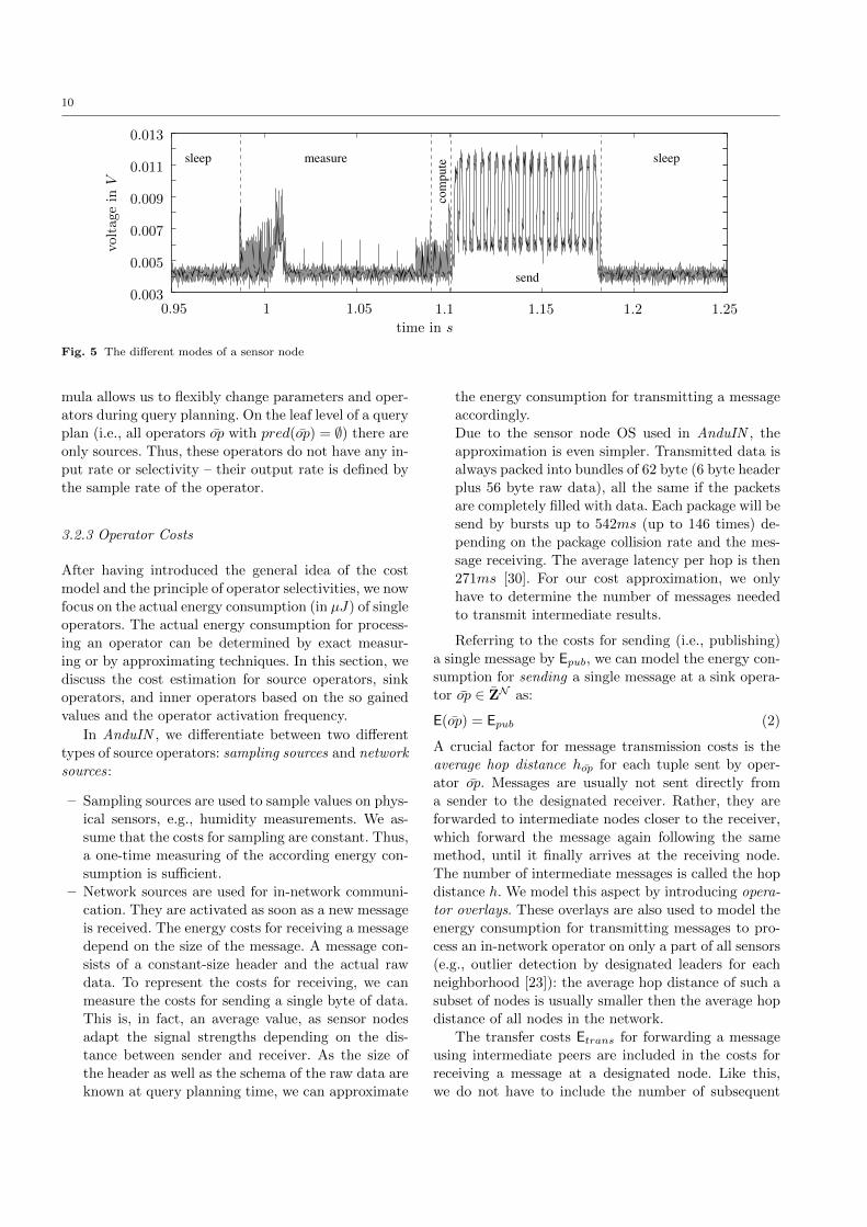
3
Frontend
Parser
Rewriter
INQP
XML
Web GUIClients
Commandline
Interface
AnduIN
DSMS
CQL Query
Query Execution Engine
Image
Library
INQP
Other
Generator
Code
Statistics
Monitor
DecomposerOptimizer &
So
urc
es
Dat
a S
trea
m
Rel
atio
ns
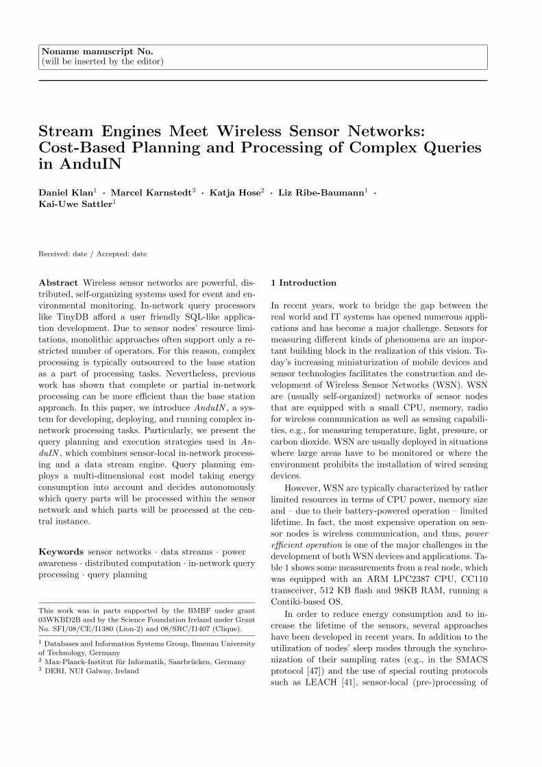
Fig. 1 AnduIN ’s Main Components and Architecture
at a central base station. Consequently, two of An-
duIN ’s main components are in-network query pro-
cessors which compute intermediate results within the
wireless sensor network and a data stream management
system which executes all remaining operations neces-
sary to fully answer a query. The data with which a
query is evaluated conforms to sensor (source) readings
and is regarded as streams of tuples. Queries themselves
may refer to relations which correspond to sets of tu-
ples that do not change over time and that are stored
at the central base station.
AnduIN ’s browser-based graphical user interface al-
lows users to graphically interact with the system by
formulating and issuing queries, monitoring results and
statistics, configuring network deployment, etc. As an
alternative, users can also decide to use the command
line interface, which provides the same functionality.
Furthermore, AnduIN provides an interface for interac-
tion with other client applications wanting to use An-
duIN ’s query processing features. Another important
component is the library of INQP operators that is used
by the code generator for network deployment.
Figure 1 shows the main components of AnduIN ’s
architecture as well as interactions between them. In
order to explain these components in more detail, we
first provide a general introduction to query processing
in AnduIN before discussing details about the query
language, in-network query processors, and the central
data stream engine.
2.1 General Steps of Query Processing
The first step of query processing is to formulate a
query, parse it, and transform it into a logical query
plan. These logical query plans consist of logical query
operators, or high-level representations of the opera-
tions that need to be executed to obtain answers to the
query. A rule-based logical optimizer reorders operators
within the logical query plan. Such a plan corresponds
to an acyclic directed graph of operators, where tuples
flow from one operator to the next according to the di-
rected edge between them [12,34]. There are three types
of operators:
– sources producing tuples,
– sinks receiving tuples, and
– inner operators receiving and producing tuples.
A query plan consists of at least one source, sev-
eral inner operators, and one sink. After logical op-
timization, the optimizer translates the logical query
plan into a set of physical execution plans and chooses
one according to the techniques discussed in Section 3.
Operators of a physical query plan adhere to a pub-
lish/subscribe mechanism to transfer tuples from one
operator to another. Using this approach is simple and
fast. Each operator could have a number of subscribers
that get result tuples from this operator. With this no
coordinator, like in SteMS [8], is necessary. Addition-
ally, we use a uniform solution on both parts of the
system, which simplifies the optimization.
A physical query plan consists of two parts: one de-
scribing which operators are to be processed within the
sensor network (Section 2.3) and one describing which
operators are to be processed by the central data stream
engine (Section 2.4). Moreover, for most logical query
operators there are at least two implementations: one
to compute the logical operator using in-network query
processors, and one to compute the logical operator at
the central data stream engine. Depending on the op-
erator and its parameters, it is possible that there are
many more alternative implementations for these two
basic variants. In-network operators are not practical
or possible in all cases. For instance, a complex data
mining algorithm, such as the frequent patter mining
approach presented by Gianella et al. [24] or the clus-
ter algorithm CluStream[2], uses synopses that will be
updated over time. The final pattern or cluster extrac-
tion will be done in batch quantities and is very expen-
sive. In these cases, the transfer of the synopses could
be more efficient than the propagation within the WSN
followed by an in-network analysis and the result prop-
agation to the central instance.
The final steps of query processing in AnduIN are
the deployment of the chosen physical query plan, the
4
processing of tuples, and the output of answers to the
query.
2.2 Query Language and Query Formulation
As AnduIN aims at combining the concepts of data
stream mining with query processing in wireless sensor
networks, a language designed for data stream systems
is insufficient. Rather, we need a query language for the
general case of formulating queries on streams of data.
AnduIN ’s query language is based on CQL [4],
which was developed in the context of the STREAM
project [5]. CQL was one of the first query languages
for processing streaming data and therefore does not
natively provide us with the full expressivity we need for
AnduIN. One of CQL’s main limitations is that queries
involving complex data mining operators cannot be ex-
pressed. Thus, we extended CQL accordingly.
In principle, CQL provides the means to formulate
queries involving synopsis operators – data structures
for aggregating data in a way that reduces memory con-
sumption and still provides sufficient information about
the original data. STREAM, however, implemented this
mainly as sliding window operators used to resolve
deadlocks between blocking operators and allows only
one operator per synopsis [7]. We extended this basic
expressivity by adding special operators corresponding
to more complex synopses – a set of parameters addi-
tionally configures their behavior and characteristics.
In comparison to sliding windows, these complex syn-
opsis operators are associated with specific algorithms
for creation, management, and updates based on the
incoming stream of tuples.
The following query selects two attributes attr1
and attr2 from the stream mystream and maintains a
synopsis on the stream itself, i.e., on all its attributes.
SELECT
attr1 , attr2
FROM mystream [ synopsis (params) ]
Table 2 shows the list of synopsis operators currently
available in AnduIN. DSMS implementations are avail-
able for all of them, INQP implementations are avail-
able for some of them, and the frequent pattern stream
synopsis is available in an implementation that comes
in two parts (DSMS and INQP) to implement the op-
erator.
In addition, AnduIN also provides the set of well-
known basic stream processing operators such as fil-
ters (including spatial filters), projection, aggregation,
grouping, and joins, for which two implementations
(DSMS and INQP) are available.
logical physical instances
operator DSMS INQP partial
adaptive burst detection [32] x x -clustering (CluStream) x - -
exponential smoothing x - -frequent pattern mining x - x
lossy counting x - -
missing detection x - -outlier detection x x -
Table 2 Synopsis operators provided by AnduIN
2.3 In-Network Query Processing
In consideration of requirements such as extensibil-
ity and flexibility, monolithic approaches, as used by
TinyDB [40], are not applicable to our problem sce-
nario. Instead, our work is based on a modular runtime
environment for sensor nodes. Similar to modular sys-
tems like PIPES [34], we provide a library of operator
implementations for constructing query plans.
AnduIN uses this library to build query or
application-specific system images for the sensor nodes.
This means that an application is developed in AnduIN
by first specifying a query (or multiple queries) run-
ning in the DSMS mode only. After successfully testing
the application, it can be deployed by decomposing the
query plans into a DSMS part and an INQP part based
on cost-based optimization techniques (see Section 3).
The INQP part is a pre-configured execution compo-
nent containing only the part of the queries which can
be processed locally on the node, i.e., operators from the
library required for these plans as well as some process
monitoring functionalities. The system image consisting
of this query execution component is flashed to the sen-
sor nodes or deployed using over-the-air-programming
techniques, if supported by the sensor platform. Al-
though this optimize-first execute-next principle is not
as flexible as a general purpose query processor running
on the sensor nodes, it minimizes resource consumption
at the nodes. Furthermore, this centralized query plan-
ning simplifies query optimization by exploiting global
information. In addition, the applications we consider
in our work are characterized by rather stable, long-
running queries not needing ad-hoc query facilities for
the sensors. Note that this does not mean that ad-hoc
queries are generally not supported. Because AnduIN
supports views on data streams, new queries can be de-
fined on top of existing views to process the sensor data
streams.
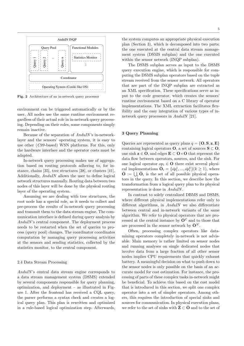
Figure 2 shows the architecture of a sensor’s runtime
environment based on a Contiki-like operating system1.
Programming the nodes and transmitting the runtime
1 http://cst.mi.fu-berlin.de/projects/ScatterWeb/
5
...
Query Pool
AnduIN INQP
Functional Modules
...
Statistics Monitor
Coordinator
Qu
ery
1
Qu
ery
2
Qu
ery
n
Operating System (Coniki like OS)
Fig. 2 Architecture of an in-network query processor
environment can be triggered automatically or by the
user. All nodes use the same runtime environment re-
gardless of their actual role in in-network query process-
ing. Depending on their roles, some components simply
remain inactive.
Because of the separation of AnduIN ’s in-network-
layer and the sensors’ operating system, it is easy to
use other (C99 -based) WSN platforms. For this, only
the hardware interface and the operator costs must be
adapted.
In-network query processing makes use of aggrega-
tion based on routing protocols adhering to, for in-
stance, chains [35], tree structures [38], or clusters [41].
Additionally, AnduIN allows the user to define logical
network structures manually. Routing data between two
nodes of this layer will be done by the physical routing
layer of the operating system.
Assuming we are dealing with tree structures, the
root node has a special role, as it needs to collect and
pre-process the results of in-network query processing
and transmit them to the data stream engine. The com-
munication interface is defined during query analysis by
AnduIN ’s central component. The deployment process
needs to be restarted when the set of queries to pro-
cess (query pool) changes. The coordinator coordinates
computation by managing query processing activities
at the sensors and sending statistics, collected by the
statistics monitor, to the central component.
2.4 Data Stream Processing
AnduIN ’s central data stream engine corresponds to
a data stream management system (DSMS) extended
by several components responsible for query planning,
optimization, and deployment – as illustrated in Fig-
ure 1. After the frontend has received a CQL query,
the parser performs a syntax check and creates a log-
ical query plan. This plan is rewritten and optimized
in a rule-based logical optimization step. Afterwards,
the system computes an appropriate physical execution
plan (Section 3), which is decomposed into two parts:
the one executed at the central data stream manage-
ment system (DSMS subplan) and the one executed
within the sensor network (INQP subplan).
The DSMS subplan serves as input to the DSMS
query execution engine, which is responsible for com-
puting the DSMS subplan operators based on the tuple
stream received from the sensor network. All operators
that are part of the INQP subplan are extracted as
an XML specification. These specifications serve as in-
put to the code generator, which creates the sensors’
runtime environment based on a C library of operator
implementations. The XML extraction facilitates flex-
ibility and the easy integration of various types of in-
network query processors in AnduIN [21].
3 Query Planning
Queries are represented as query plans q = O,S, z,Econtaining logical operators O, a set of sources S ⊂ O,
one sink z ∈ O, and edges E ⊂ O×O that represent the
data flow between operators, sources, and the sink. For
one logical operator opi ∈ O there exist several physi-
cal implementations Oi = op1i , ..., op
ki (k ≥ 1), where
O :=⋃i Oi is the set of all possible physical opera-
tors in the query. In this section, we describe how the
transformation from a logical query plan to its physical
representation is done in AnduIN .
In contrast to solely centralized DBMS and DSMS,
where different physical implementations refer only to
different algorithms, in AnduIN we also differentiate
between central and in-network variants of the same
algorithm. We refer to physical operators that are pro-
cessed at the central instance by OL and to those that
are processed in the sensor network by ON .
Often, processing complex operators like data-
mining operators completely in-network is not advis-
able. Main memory is rather limited on sensor nodes
and running analyses on single dedicated nodes that
involve data from a large fraction of all other sensor
nodes implies CPU requirements that quickly exhaust
battery. A meaningful decision on what to push down to
the sensor nodes is only possible on the basis of an ac-
curate model for cost estimation. For instance, the pro-
cessing of parts of these complex tasks in-network might
be beneficial. To achieve this based on the cost model
that is introduced in this section, we split one complex
operator into a set of simpler operators. Among oth-
ers, this requires the introduction of special sinks and
sources for communication. In physical execution plans,
we refer to the set of sinks with Z ⊂ O and to the set of
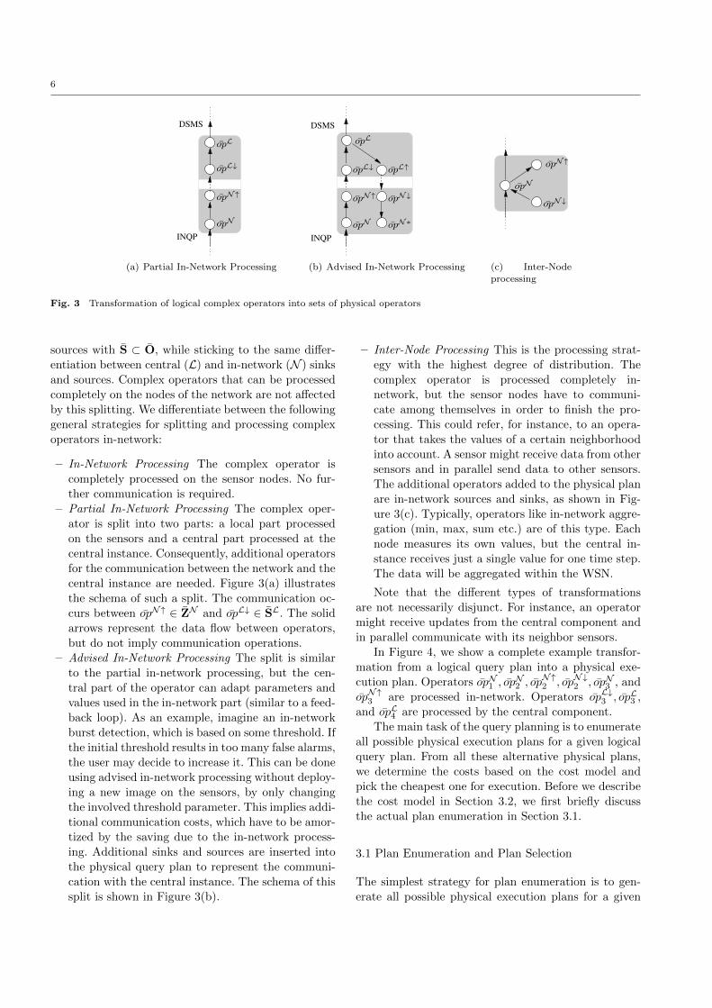
6
DSMS
INQP
opL↓
opN↑
opL
opN
(a) Partial In-Network Processing
INQP
DSMS
opL
opL↓ opL↑
opN↑ opN↓
opN opN∗
(b) Advised In-Network Processing
opN↑
opN↓
opN
(c) Inter-Node
processing
Fig. 3 Transformation of logical complex operators into sets of physical operators
sources with S ⊂ O, while sticking to the same differ-
entiation between central (L) and in-network (N ) sinks
and sources. Complex operators that can be processed
completely on the nodes of the network are not affected
by this splitting. We differentiate between the following
general strategies for splitting and processing complex
operators in-network:
– In-Network Processing The complex operator is
completely processed on the sensor nodes. No fur-
ther communication is required.
– Partial In-Network Processing The complex oper-
ator is split into two parts: a local part processed
on the sensors and a central part processed at the
central instance. Consequently, additional operators
for the communication between the network and the
central instance are needed. Figure 3(a) illustrates
the schema of such a split. The communication oc-
curs between opN↑ ∈ ZN and opL↓ ∈ SL. The solid
arrows represent the data flow between operators,
but do not imply communication operations.
– Advised In-Network Processing The split is similar
to the partial in-network processing, but the cen-
tral part of the operator can adapt parameters and
values used in the in-network part (similar to a feed-
back loop). As an example, imagine an in-network
burst detection, which is based on some threshold. If
the initial threshold results in too many false alarms,
the user may decide to increase it. This can be done
using advised in-network processing without deploy-
ing a new image on the sensors, by only changing
the involved threshold parameter. This implies addi-
tional communication costs, which have to be amor-
tized by the saving due to the in-network process-
ing. Additional sinks and sources are inserted into
the physical query plan to represent the communi-
cation with the central instance. The schema of this
split is shown in Figure 3(b).
– Inter-Node Processing This is the processing strat-
egy with the highest degree of distribution. The
complex operator is processed completely in-
network, but the sensor nodes have to communi-
cate among themselves in order to finish the pro-
cessing. This could refer, for instance, to an opera-
tor that takes the values of a certain neighborhood
into account. A sensor might receive data from other
sensors and in parallel send data to other sensors.
The additional operators added to the physical plan
are in-network sources and sinks, as shown in Fig-
ure 3(c). Typically, operators like in-network aggre-
gation (min, max, sum etc.) are of this type. Each
node measures its own values, but the central in-
stance receives just a single value for one time step.
The data will be aggregated within the WSN.
Note that the different types of transformations
are not necessarily disjunct. For instance, an operator
might receive updates from the central component and
in parallel communicate with its neighbor sensors.
In Figure 4, we show a complete example transfor-
mation from a logical query plan into a physical exe-
cution plan. Operators opN1 , opN2 , op
N↑2 , opN↓2 , opN3 , and
opN↑3 are processed in-network. Operators opL↓3 , opL3 ,
and opL4 are processed by the central component.
The main task of the query planning is to enumerate
all possible physical execution plans for a given logical
query plan. From all these alternative physical plans,
we determine the costs based on the cost model and
pick the cheapest one for execution. Before we describe
the cost model in Section 3.2, we first briefly discuss
the actual plan enumeration in Section 3.1.
3.1 Plan Enumeration and Plan Selection
The simplest strategy for plan enumeration is to gen-
erate all possible physical execution plans for a given
7
op3
op4
op2
op1
(a)
opN1
opN3
opN↓2
opN↑2
opN↑3
opL4
opL3 ↓
opL3
opN2
(b)
DSMS
central
instance
result
sensor node
with
plan
INQP
execution
(c)
Fig. 4 Transformation of a logical query plan (a) into a physical execution plan (b) and the final execution on the sensor nodes (c)
logical plan, in consideration of alternative implemen-
tations for logical operators and associative and com-
mutative groups and operators (e.g., join order). Lit-
erature proposes two basic strategies for physical plan
construction [48]: bottom-up and top-down. The for-
mer begins construction at the logical operators repre-
senting the sources and constructs plans by considering
variations of all operators in upper levels of the logi-
cal query plan. The latter strategy starts constructing
plans at the sink and traverses the logical plan down to
the sources. However, constructing all possible physical
query plans can be very expensive. Thus, a common
approach is to apply heuristics that limit the number
of query plans.
There exist many proposals in standard database
literature for alternatives to implement plan enumera-
tion, such as dynamic programming, hill climbing, etc.
The actual approach used and the resulting costs are
out of the scope of this work. For details we refer to [48].
However, it is important to understand that the result-
ing costs have less impact in the streaming scenario of
DSMS than in traditional DBMS. In DBMS, the costs
are an important part of the overall costs of one-shot
queries. In contrast, the continuous queries of DSMS
clearly shift the importance to the efficient processing
of the actual query. The overhead of plan enumeration
becomes the less important the longer a query is run-
ning. Of more importance in this setup is an adaptive
query planning. In the context of continuous queries it
is very important to be able adapt to changing situa-
tions, such as increasing stream or anomaly rates, and
a changing number of parallel queries. However, the fo-
cus of this work is on a cost model that generally sup-
ports in-network query processing. Adaptive planning
is a next step that justifies an own exhaustive work.
Plan enumeration in AnduIN works in a bottom-up
fashion and applies two heuristics to limit the num-
ber of physical query plans. The first heuristic is that
once a partial plan contains the “crossover” from in-
network query processing to processing at the central
data stream engine, we do not consider any plans that
introduce further crossovers back to in-network query
processing, because these plans are too expensive.
The second heuristic regards the limited memory of
the sensor nodes. Both main and flash memory are lim-
ited. Thus, for the plan enumeration, the system has
to compute the flash memory and the expected main
memory consumption for each plan. Thus, for the trans-
formation of a logical operator into a physical one the
system approximates the expected memory consump-
tion. In case the system estimates that the memory
will be exceeded, the operator is placed on the central
instance. This approach is quite simple and does not
guarantee that the most efficient plan will be found. In
future work, we plan to use the most efficient plan by
also considering the memory space.
After plan enumeration, we need to select one plan
for execution. The standard approach is to estimate the
costs for each of these physical query plans (Section 3.2)
and choose the one promising the least costs. The most
important criterion in sensor networks is energy con-
sumption. Thus, most cost models measure costs in
terms of energy consumption. However, there are fur-
ther criteria that play an important role for the decision
which plan to choose, e.g., quality-of-service parameters
like output rate.
8
When we have multiple criteria that we want to base
our choice on, we face a typical instance of the multi-
criteria decision making problem. A basic solution to
this problem is to define a weight for each criterion and
use the sum over all weighted criteria to determine the
best plan. The definition of the weights is a crucial task.
An alternative approach towards multicriteria decision
making is to determine the pareto optimum, also re-
ferred to as skyline [11] or maximal vector problem [25,
43].
The main idea is that only plans that are not “domi-
nated” by another plan are part of the pareto optimum.
Plan A dominates another plan B if A is not worse than
B with respect to all criteria and better with respect to
at least one criterion.
Formally, a plan p is said to dominate another plan
q, denoted as p ≺ q, if (1) for each criterion di, pi is
ranked at least as good as qi and (2) for at least one
criterion dj , pj is ranked better than qj . The pareto
optimum is a set P(S) ⊆ S for which no plan in P(S) is
dominated by any other plan contained in P(S) – with
S denoting the set of all considered candidate plans.
For instance, assuming that plan A requires less en-
ergy than plan B and both plans have the same output
rate, then plan B is dominated and therefore not part
of the pareto optimum. Intuitively, the pareto optimum
can be understood as the set of all plans that represent
”good“ combinations of all criteria without weighting
them. Based on this set of plans, the user can choose
a plan that meets her preferences. To limit the amount
of user interaction, we can try to derive weights for the
criteria based on the choices of plans from the pareto
optimum made by the user in the past, so that in the
future no (or less) user interaction will be required.
Instead of creating all possible physical query plans
first and determining the pareto optimum afterwards,
we can also construct the pareto optimum incremen-
tally during plan enumeration. Therefore, we apply a
depth-first approach for plan construction. Thus, we
obtain the first complete physical query plans after a
short time. Whenever we have produced an alternative
physical query plan, we check it for dominance by the
plans of the current pareto optimum and add the new
plan if possible. During plan construction we derive a
variety of plans based on the same incomplete phys-
ical query plan. Therefore, we already compare these
incomplete plans to the plans of the pareto optimum.
The idea is that if the incomplete physical query plan
is already dominated by a plan contained in the pareto
optimum, then all plans generated based on this in-
complete plan cannot be part of the pareto optimum.
Thus, we can reduce the number of plans that need to
be generated.
3.2 Cost Model
There are several cost factors important in wireless sen-
sor networks. These different factors have to form the
dimensions of any cost model for processing queries.
The most important ones are:
1. energy consumption
2. main memory
3. data quality
4. output rate or throughput
We propose a cost model that is designed to deal with
multiple dimensions. Clearly, the most important di-
mension is the energy consumption, as battery is the
most limited resource on wireless sensor nodes. Thus,
cost model and query planning proposed in this work
are focused on minimizing the resulting energy con-
sumption. To illustrate the handling of multiple dimen-
sions, we integrate the output rate into the discussions.
The output rate reflects the amount of result data pro-
duced per time step and depends on the computation
time per tuple. Thus, it reflects the overall performance
of query processing, involves costs for disk access and
similar, and is related to the blocking behavior of op-
erators, and therefore to data quality. This choice re-
sults in a particularly illustrative and easy to under-
stand model, while highlighting the general principle
of multidimensional cost-based query planning. It is
particularly illustrative as it also involves the central
component. DSMS usually process several continuous
queries that have to share resources. To enable this,
the costs per query have to be kept low and, more im-
portant, have to be dynamically adjustable. Thus, after
discussing the in-network costs in Sections 3.2.1–3.2.4,in Section 3.2.5 we briefly discuss the costs occurring in
the central component.
Main memory is a crucial factor as well, particu-
larly in the context of multiple continuous queries that
run in parallel. However, at the current state AnduIN
works fine with the memory heuristic introduced in Sec-
tion 3.1. In future work, we will integrate this dimen-
sion in the cost model, together with approaches for
resource- and quality-aware processing of queries. [22]
is one of the first works that discusses the dependencies
between result quality and resource awareness.
Data quality was a driving factor for the design of
the Aurora DSMS [12]. Due to the wealth of existing
research in this area, we do not focus on this aspect in
more detail. For the time being, in AnduIN we expect
operators to produce results with the desired quality,
e.g., no parts of input data are discarded by load shed-
ding [9] or similar techniques. This assumption might
not hold in all situations in practice. However, the de-
scription of the cost model and query planning would
9
become significantly more complicated, so that this as-
sumption is mainly for the sake of understandability.
Load shedding and similar techniques can be integrated
without changing the essence of the proposed approach
– we indicate it accordingly where appropriate.
The cost model is not designed to reflect exact costs
of different operator implementations and execution
plans. Rather, it is designed to accurately reflect the
differences and relations between the available alterna-
tives. Further, the aim of the cost model is to assess the
overall costs occurring in the sensor network.
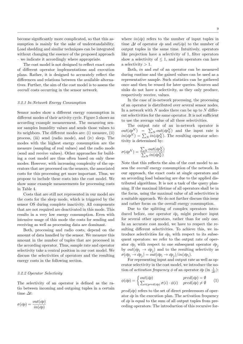
3.2.1 In-Network Energy Consumption
Sensor nodes show a different energy consumption in
different modes of their activity cycle. Figure 5 shows an
according example measurement. The measuring sen-
sor samples humidity values and sends those values to
its neighbors. The different modes are: (i) measure, (ii)
process, (iii) send (radio mode), and (iv) sleep. The
modes with the highest energy consumption are the
measure (sampling of real values) and the radio mode
(send and receive values). Other approaches for build-
ing a cost model are thus often based on only these
modes. However, with increasing complexity of the op-
erators that are processed on the sensors, the associated
costs for this processing get more important. Thus, we
propose to include these costs into the cost model. We
show some example measurements for processing costs
in Table 4.
Costs that are still not represented in our model are
the costs for the sleep mode, which is triggered by the
sensor OS during complete inactivity. All components
that are not required are deactivated in this mode. This
results in a very low energy consumption. Even with
intensive usage of this mode the costs for sending and
receiving as well as processing data are dominant.
Both, processing and radio costs, depend on the
amount of data handled by the sensor. We measure this
amount in the number of tuples that are processed in
the according operator. Thus, sample rate and operator
selectivity take a central position in our cost model. We
discuss the selectivities of operators and the resulting
energy costs in the following section.
3.2.2 Operator Selectivity
The selectivity of an operator is defined as the ra-
tio between incoming and outgoing tuples in a certain
time ∆t:
σ(op) =out(op)
in(op)
where in(op) refers to the number of input tuples in
time ∆t of operator op and out(op) to the number of
output tuples in the same time. Intuitively, operators
like projection have a selectivity of 1, filter operators
show a selectivity of ≤ 1, and join operators can have
a selectivity > 1.
Both, in and out of an operator can be measured
during runtime and the gained values can be used as a
representative sample. Such statistics can be gathered
once and then be reused for later queries. Sources and
sinks do not have a selectivity, as they only produce,
respectively receive, values.
In the case of in-network processing, the processing
of an operator is distributed over several sensor nodes.
In a network with N nodes there can be up to N differ-
ent selectivities for the same operator. It is not sufficient
to use the average value of all these selectivities.
The output rate of an in-network operator is
out(opN ) =∑N out(op
NN ) and the input rate is
in(opN ) =∑N in(opNN ). The resulting operator selec-
tivity is determined by:
σ(opN ) =
∑N out(op
NN )∑
N in(opNN )
Note that this reflects the aim of the cost model to as-
sess the overall energy consumption of the network. In
our approach, the exact costs at single operators and
an according load balancing are due to the applied dis-
tributed algorithms. It is not a task of the query plan-
ning. If the maximal lifetime of all operators shall be in
the focus, using the maximal value of all selectivities is
a suitable approach. We do not further discuss this issue
and rather focus on the overall energy consumption.
Due to the splitting of complex operators intro-
duced before, one operator opi might produce input
for several other operators, rather than for only one.
In an accurate cost model, we have to respect the re-
sulting different selectivities. To achieve this, we in-
troduce selectivities for opi with respect to its subse-
quent operators: we refer to the output rate of oper-
ator opi with respect to one subsequent operator opjby out(opi → opj) and to the resulting selectivity as
σ(opi → opj) = out(opi → opj)/in(opi).
For representing input and output rate as well as op-
erator selectivity in the cost model, we introduce the no-
tion of activation frequency φ of an operator op (in 1∆t ):
φ(op) =
out(op) pred(op) = ∅∑i∈pred(op) σ(i) · φ(i) pred(op) 6= ∅ (1)
pred(op) refers to the set of direct predecessors of oper-
ator op in the execution plan. The activation frequency
of op is equal to the sum of all output tuples from pre-
ceding operators. The introduction of this recursive for-
10
sleep measure sleep
send
compute
time in s
0.003
0.005
0.007
0.009
0.011
0.95 1 1.05 1.1 1.15 1.2 1.25
0.013
volt
age
inV
Fig. 5 The different modes of a sensor node
mula allows us to flexibly change parameters and oper-
ators during query planning. On the leaf level of a query
plan (i.e., all operators op with pred(op) = ∅) there are
only sources. Thus, these operators do not have any in-
put rate or selectivity – their output rate is defined by
the sample rate of the operator.
3.2.3 Operator Costs
After having introduced the general idea of the cost
model and the principle of operator selectivities, we now
focus on the actual energy consumption (in µJ) of single
operators. The actual energy consumption for process-
ing an operator can be determined by exact measur-
ing or by approximating techniques. In this section, we
discuss the cost estimation for source operators, sink
operators, and inner operators based on the so gained
values and the operator activation frequency.
In AnduIN , we differentiate between two different
types of source operators: sampling sources and network
sources:
– Sampling sources are used to sample values on phys-
ical sensors, e.g., humidity measurements. We as-
sume that the costs for sampling are constant. Thus,
a one-time measuring of the according energy con-
sumption is sufficient.
– Network sources are used for in-network communi-
cation. They are activated as soon as a new message
is received. The energy costs for receiving a message
depend on the size of the message. A message con-
sists of a constant-size header and the actual raw
data. To represent the costs for receiving, we can
measure the costs for sending a single byte of data.
This is, in fact, an average value, as sensor nodes
adapt the signal strengths depending on the dis-
tance between sender and receiver. As the size of
the header as well as the schema of the raw data are
known at query planning time, we can approximate
the energy consumption for transmitting a message
accordingly.
Due to the sensor node OS used in AnduIN , the
approximation is even simpler. Transmitted data is
always packed into bundles of 62 byte (6 byte header
plus 56 byte raw data), all the same if the packets
are completely filled with data. Each package will be
send by bursts up to 542ms (up to 146 times) de-
pending on the package collision rate and the mes-
sage receiving. The average latency per hop is then
271ms [30]. For our cost approximation, we only
have to determine the number of messages needed
to transmit intermediate results.
Referring to the costs for sending (i.e., publishing)
a single message by Epub, we can model the energy con-
sumption for sending a single message at a sink opera-
tor op ∈ ZN as:
E(op) = Epub (2)
A crucial factor for message transmission costs is the
average hop distance hop for each tuple sent by oper-
ator op. Messages are usually not sent directly from
a sender to the designated receiver. Rather, they are
forwarded to intermediate nodes closer to the receiver,
which forward the message again following the same
method, until it finally arrives at the receiving node.
The number of intermediate messages is called the hop
distance h. We model this aspect by introducing opera-
tor overlays. These overlays are also used to model the
energy consumption for transmitting messages to pro-
cess an in-network operator on only a part of all sensors
(e.g., outlier detection by designated leaders for each
neighborhood [23]): the average hop distance of such a
subset of nodes is usually smaller then the average hop
distance of all nodes in the network.
The transfer costs Etrans for forwarding a message
using intermediate peers are included in the costs for
receiving a message at a designated node. Like this,
we do not have to include the number of subsequent
11
operators in the sink operator – it is implicitly observed
by the number of receiving source operators. We assume
that the costs for sending a single message are equal to
the costs Erecv for receiving it, i.e., Epub = Erecv. Thus,
costs for receiving a message at a designated network
source operator op ∈ SN are:
E(op) = Epub + Etrans(op)
The transfer costs for operator op are:
Etrans(op) = (Epub + Erecv) · (hop − 1)
= 2 · Epub · (hop − 1)
Usually, the sensor nodes are in the sleep mode. To
receive a message, they have to be reactivated, which
results in wake-up costs. As these costs are very low
and are comparable to the usual “noise” of a sensor’s
energy consumption (they can be identified in Figure 5
at the very short switch phases between different sensor
modes), we do not capture them explicitly in the cost
model.
The costs for transmitting messages to the central
instance are estimated analogously. The sending node
pushes the message into the network and intermedi-
ate nodes care for forwarding it to the central instance.
The costs for the sink operator responsible for trans-
mitting data to the central instance are estimated by
Equation 2. In contrast, the receiving source operator
at the central instance does not involve any energy con-
sumption. Thus, the costs for a central source operator
op ∈ SL are:
E(op) = Etrans(op) = 2 · Epub · (hop − 1)
One approach to determining the average hop dis-
tance for the whole network is to send a broadcast
message from the central instance. Every node that
forwards this message increments a counter. After all
nodes at the leaf level of the network received it, they
send a response message back to the central instance.
On the way back, the counters of the original message
are aggregated. Finally, the central instance can deter-
mine the hop distance of the whole network from the
aggregated value, and can determine the average hop
distance taking the number of sensor nodes into ac-
count. Similar approaches and statistics have to be used
to determine the average hop distance for an overlay
network used for processing a complex operator. With
a known sample rate for each source, it is then possible
to determine the average hop distance per tuple.
Another approach is the usage of tree or cluster hier-
archies, similar to TAG [38] or LEACH [41]. In this ap-
proach, each parent node receives the number of nodes
and hops from its children, aggregates them and for-
wards the result to its own parent. The hop distance is
counted starting from the leaf nodes. The main prob-
lem of this approach is the maintenance overhead. In
the case of a node failure or movement, a whole subtree
has to be updated. In the case of the previous simple
approach, the counting will be initialized completely
new each time. Dependent on the dynamic behavior of
the sensor network and the checkup time, the first or
the second approach will be more efficient. Neverthe-
less, both techniques have no influence on the actual
query processing costs.
A main problem in modeling the communication
costs is that we have to assume some communication
topology. Events like packet loss and retransmissions
are usually of non-deterministic nature and impossi-
ble to predict accurately. However, as in any database
cost model, the aim is not to model processing costs
exactly. Rather, the aim is to accurately estimate dif-
ferences and trends between alternatives. As such, it
is sufficient to model average costs, resulting from the
unreliability of wireless communication, in the activa-
tion frequencies of source operators and in the average
hop distance. The required statistics can be learned and
optionally adapted over time.
For estimating the costs of inner operators we have
to take the processing costs of the operator implemen-
tations into account. As mentioned before, we deter-
mine these as processing costs per input tuple. For al-
gorithms with constant costs (filter, projection, sum,
average, etc.) it is sufficient to measure these costs only
once. For operators with non-constant costs we have to
approximate them accordingly. We use an example to
demonstrate the approximation of the simple minimum
operator opmin.
Example 3.1 The minimum operator returns the
minimum over the last k values of a data stream. w de-
notes the maximum possible elements of the window.
A newly inserted value will be compared with the cur-
rent minimum. In case the new value is smaller then
the current minimum, the operator sets the new value
as minimum and inserts it into the window. The inser-
tion displaces the oldest element of the window. In case
the replaced value does not correspond to the current
minimum the processing is finished. Otherwise, the win-
dow must be searched until a new minimum has been
found. In the worst case, the operator has to check all
w elements of the window.
In order to approximate the execution costs for this
operator we can use two reference measurements E1 and
E2 with a window size of w1 and w2 respectively. With
this, we can approximate the costs for an arbitrary win-
12
9
7
36
5
4
1
2
8
base station
10
logical plan physical plan
¯connNA,B
¯connLA,B
σNB>x
ζA,B
σB>x
ζA,B
Fig. 6 Example 1
Symbol Operator
ζA,B operator sampling values A and B
σNB>x operator filtering B > x
¯connN↑A,B sink sending values A and B
¯connL↓A,B source receiving values A and B
¯aggNB operator aggregating B
¯aggN↓A,B in-network source for ¯aggNB¯aggN↑A,B in-network sink for ¯aggNB
¯connN↑¯aggA,Bsink for ¯aggNB sending to central instance
¯connL↓¯aggA,Bsource for ¯aggNB at central instance
Table 3 Example operators
dow size by
E(opmin, w) =
(E2 − E1
w2 − w1
)· w −
(E2 − E1
w2 − w1
)· w1 + E1
In most cases, it is possible to define a similar approxi-
mation for operators with non-constant costs (e.g., dif-
ferent join implementations, aggregations). Neverthe-
less, in case an approximation is not possible (for in-
stance, for complex operators like clustering or frequent
pattern mining) we can use some observed data for the
cost estimation.
3.2.4 Costs of Execution Plans
Based on operator activation frequency, operator selec-
tivity, and operator processing costs, we can estimate
the costs for a physical execution plan q on one sensor
node in the time ∆t as follows:
Enode(q) =∑op∈qN
E(op) · φ(op) (3)
In the following, we illustrate the whole cost estimation
on the basis of two examples. Table 3 summarizes the
operators used in the examples.
Example 3.2 On each sensor node operator
ζA,B samples 5 times per minute. For the example net-
work from Figure 6, consisting of 10 battery powered
nodes, this means we have 50 samples per minute, i.e.,
out(ζA,B) = 50. We assume operator σNB>x has a se-
lectivity of 0.5, i.e., in average only each second tuple
passes the operator. The average hop distance of the
whole network is (1+2+2+2+3+3+3+4+4+4)/10 =
2.8. With this, the overall power consumption can be
estimated by:
E(q1) = 50 · E(ζA,B) + 50 · E(σNB>x)
+50 · 0.5 · E( ¯connN↑A,B) + 50 · 0.5 · E( ¯connL↓A,B)
= 50 · (E(ζA,B) + E(σNB>x))
+25 · (Epub + Etrans( ¯connL↓A,B))
= 50 · (E(ζA,B) + E(σNB>x))
+25 · (Epub + 2 · Epub · (h ¯connL↓A,B− 1))
= 50 · (E(ζA,B) + E(σNB>x)) + 25 · 4.6 · Epub
Example 3.3 In this example, we illustrate an in-
network aggregation, similar to TAG [38]. Inner nodes
of the network wait for tuples from their child nodes and
aggregate these with their own measurements before
forwarding the aggregated values towards the central
instance. The query in Figure 7 shows the in-network
representation in the AnduIN operator model. The in-
network aggregation operator ¯aggNB has an additional
network source ¯aggN↓A,B and an additional sink ¯aggN↑A,Bfor communicating with the neighbor nodes.
As the same network topology as in the first exam-
ple is used, we also have 10 sensor nodes and an aver-
age hop distance of 2.8. Each node samples 5 times per
minute, i.e., out(ζA,B) = 50. The outrate of ¯aggNB with
reference to ¯aggN↑A,B is 45 (each node, except node 2,
forwards 5 tuples). Thus, operator ¯aggN↓A,B produces 45
tuples (inner nodes receive the results from the neigh-
bors by this operator). The outrate of ¯aggNB with ref-
erence to ¯connN↑¯aggA,Bis 5, since only node 2 has to for-
ward the final aggregate (5 times per minute) to the
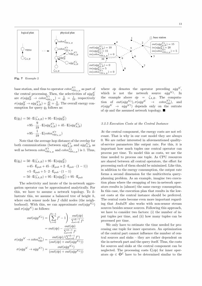
13
7
36
5
4
1
8
base station
9
physical planlogical plan
10
2
out( ¯aggN↓A,B) = 0in( ¯aggNB ) = 5in( ¯connN↑¯aggA,B
) = 0
out( ¯aggN↓A,B) = 10in( ¯aggNB ) = 15in( ¯connN↑¯aggA,B
) = 0
out( ¯aggN↓A,B) = 15in( ¯aggNB ) = 20in( ¯connN↑¯aggA,B
) = 5
ζA,B
aggB
¯connL¯aggA,B
ζA,B
¯aggN↓A,B
¯aggNB
¯aggN↑A,B
¯connN↑¯aggA,B
Fig. 7 Example 2
base station, and thus to operator ¯connN↑¯aggA,Bas part of
the central processing. Then, the selectivities of ¯aggNBare σ( ¯aggNB → ¯connN↑¯aggA,B
) = 595 = 1
19 , respectively
σ( ¯aggNB → ¯aggN↑A,B) = 4595 = 9
19 . The overall energy con-
sumption for query q2 follows as:
E(q2) = 50 · E(ζA,B) + 95 · E( ¯aggNB )
+95 · 9
19· E( ¯aggN↑A,B) + 45 · E( ¯aggN↓A,B)
+95 · 1
19· E( ¯connN↑¯aggA,B
)
Note that the average hop distance of the overlay for
both communications (between ¯aggN↑A,B and ¯aggN↓A,B as
well as between ¯connN↑¯aggA,Band ¯connL↓¯aggA,B
) is 1. Thus,
E(q2) = 50 · E(ζA,B) + 95 · E( ¯aggNB )
+45 · Epub + 45 · (Epub + 2 · Epub · (1− 1))
+5 · Epub + 5 · 2 · Epub · (1− 1)
= 50 · E(ζA,B) + 95 · E( ¯aggNB ) + 95 · Epub
The selectivity and inrate of the in-network aggre-
gation operator can be approximated analytically. For
this, we have to assume a network topology. To il-
lustrate this, we assume a balanced tree of height h,
where each sensor node has f child nodes (the neigh-
borhood). With this, we can approximate out( ¯aggN↓)
and σ( ¯aggN ) as follows:
out( ¯aggN↓) =
(h−1∑i=0
f i − 1
)· out(op)∑h−1
i=0 fi
= out(op)− out(op)∑h−1i=0 f
i
σ( ¯aggN → ¯connN↑¯agg) =out(op)/(
∑h−1i=0 f
i)
(out(op) + out( ¯aggN↓))
σ( ¯aggN → ¯aggN↑) =out( ¯aggN↓)
(out(op) + out( ¯aggN↓))
where op denotes the operator preceding ¯aggN ,
which is not the network source ¯aggN↓. In
the example above op = ζA,B . The computa-
tion of out( ¯aggN↓), σ( ¯aggN → ¯connN↑¯agg), and
σ( ¯aggN → ¯aggN↑) depends only on the outrate
of op and the assumed network topology.
3.2.5 Execution Costs at the Central Instance
At the central component, the energy costs are not rel-
evant. That is why in our cost model they are always
0. We are rather interested in aforementioned quality-
of-service parameters like output rate. For this, it is
important how much tuples one central operator can
process per time. To model this as costs, we use the
time needed to process one tuple. As CPU resources
are shared between all central operators, the effort for
processing each of them should be minimized. Like this,
in addition to the energy consumption, the output rate
forms a second dimension for the multicriteria query-
planning problem. As an example, imagine two execu-
tion plans where the swapping of two in-network oper-
ators results in (almost) the same energy consumption.
In this case, the execution plan that results in the low-
est costs at the central instance should be preferred.
The central costs become even more important regard-
ing that AnduIN also works with non-sensor stream
sources besides sensor sources. Following this approach,
we have to consider two factors: (i) the number of in-
put tuples per time, and (ii) how many tuples can be
processed per time.
We only have to estimate the time needed for pro-
cessing one tuple for inner operators. An optimization
of the central part cannot influence the number of cen-
tral sources and sinks – they are rather dependent on
the in-network part and the query itself. Thus, the costs
for sources and sinks at the central component can be
neglected. The processing costs C(op) for inner oper-
ators op ∈ OL have to be determined similar to the
14
energy costs of in-network operators. Operators with
constant costs can be measured once, while costs for
operators with a non-constant overhead have to be ap-
proximated. It is important to observe that the costs
are dependent on the underlying system. All measures
have to be taken on the same system.
Our approach for estimating the overall costs at the
central instance are based on an idea similar to the effi-
ciency in physics. We determine costs that have no unit,
by multiplying the time C(op) needed to process one
tuple with the activation frequency φ(op). The lower
these costs summed over all central operators are, the
less CPU resources are needed. Are the operator selec-
tivities, the number of tuples produced by the sources,
and the costs for processing single operators known, we
can estimate the overall costs for processing an execu-
tion plan at the central component as:
C(q) =∑
op∈qL\S\z
C(op) · φ(op) (4)
The number of input tuples can be determined using
Equation 1. In the multicriteria query planning prob-
lem, these central costs have to be minimized.
A value of C(op) ·φ(op) > 1 means that the operator
op cannot process all input tuples in time, which results
in a blocking behavior. As such a blocking has to be
resolved by reducing the input rate (e.g., by reducing a
sample rate or applying load shedding), this should be
avoided. We assume that there is no blocking behavior
at any of the central operators. For scenarios where
this assumption might be wrong, we have to add an
additional criteria to the query-planning problem, suchas maxop∈qL\S\z ≤ 1.
Note that the suitability of the pareto approach over
the two cost dimensions as introduced here is limited to
a subset of all planning problems, such as the example
mentioned in the beginning of this section. To enable it
meaningfully in general, energy costs as well as process-
ing costs have to be determined for the in-network part
as well as for the central component. The cost model
introduced for in-network energy consumption is suited
to easily integrate the processing power of the sensors.
This affects the output and input rate of inner opera-
tors as well as their selectivity. An according approach
could be based on the ideas from [49]. The cost model
works as before, only the parameters have to be adapted
accordingly. We do not provide more details on this.
This completes the cost model. As described in Sec-
tion 3.1, the task of the query planner is now to enu-
merate all possible execution plans and to decide on
one of them. This has to be done with respect to the
relevant dimensions: overall energy consumption in the
network and output rate (i.e., central processing costs).
This can be arbitrarily extended, for instance, by addi-
tionally regarding memory consumption.
4 Evaluation
In this section, we show the general suitability of the
proposed query planning to enable ordering of physical
execution plans based on estimating their real costs.
The presented cost model depends on two parameters:
the costs for the execution of an operator and its ac-
tivation frequency. For this, we present in Section 4.1
the measurements for some INQP and DSMS operators
integrated in AnduIN . Afterwards, we use an example
to show the applicability of estimating the costs for an
operator with non-constant complexity. Based on these
results, we compare the predicted in-network costs with
the real power consumption of a query in AnduIN .
4.1 Operator Costs
In-Network Processing Costs For our experiments, we
used sensor nodes equipped with MSBA2 boards and
an ARM LPC2387 processor, a CC1100 transceiver,
512KB Flash, 98 KB RAM, an SD-card reader, and a
camera module. The SD-card of each sensor node con-
tains a small configuration for the customization of the
query execution (e.g., a unique node identifier). In or-
der to measure power consumption, we use two nodes:
one base station node, connected to the DSMS part ofAnduIN , and a battery-powered sensor node observed
by a digital storage oscilloscope. The oscilloscope mea-
sures the fall of voltage over a resistor of 1Ω (less than
3% discrepancy), installed between the power source
(the battery) and the sensor node’s main board. The
board itself requires a voltage of at least 3.3V . Since
the battery provides up to 4.3V , the added resistor has
no effect on the nodes’ functionality.
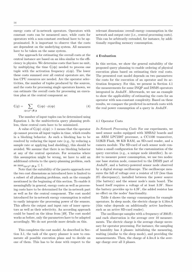
Table 4 shows the energy consumption for example
operators. In sleep mode, the electric charge is 4.16mA
(this value depends on additionally active hardware,
such as an active SD-card reader).
The oscilloscope samples with a frequency of 20kHz
and each observation is the average over 10 measure-
ments. The electric charge is the average charge neces-
sary for operator processing. For instance, the sampling
of humidity has 3 phases: initializing the measuring,
waiting (similar to the sleep mode), and providing the
measurements. Then, the charge of 4.3mA is the aver-
age charge over all 3 phases.
15
electric consumed
time charge energyoperator in ms in mA in µJ
sample (temp) 264.5 4.3 3753.4
sample (hum) 114 4.4 1655.3sample (temp + hum) 359 4.0 4738.8
send (init) 2.3 7.9 61,7
send (62B - 1Push) 3.6 8.4 99.7avg send 271 - 7344.8
outlier detection 6.1 5.5 110.7
FPP Tree Op (L1) 18.9 7.2 654.7FPP Tree Op (L2) 65.8 6.2 1346.4
FPP Tree Op (L3) 55.2 7.6 1384.4
Table 4 Example energy consumption of in-network operators.
window size
Operator 1 10 100
projection 126 - -filter 136 - -
aggregation 173 170+332 166 + 367
grouping - 139+909 141 + 956nested loop join - 734+1211+1220 6035+9031+8657
hash join - 342+875+817 1225+3654+3600
outlier detection - 178 393
Table 5 Example computation time for one tuple (time per
tuple in µs).
Output rate: computation time per tuple For measur-
ing the processing times, we extended AnduIN ’s DSMS
component by a statistics monitor. The statistics mon-
itor registers the number of incoming and outgoing tu-
ples per node and observes the activation times of all
operators. With this, we can calculate the computation
time of each operator necessary for processing a single
tuple.
Table 5 shows the computation times for exampleoperators in AnduIN ’s DSMS component. Each compu-
tation time for window-based operators has been split
into either two or three parts. The first value denotes
the operator processing time (without the window look-
up) and the remaining values denote the time necessary
for the window look-up(s).
These measurements show the general applicabil-
ity of evaluating single operators with respect to power
consumption or tuple computation time.
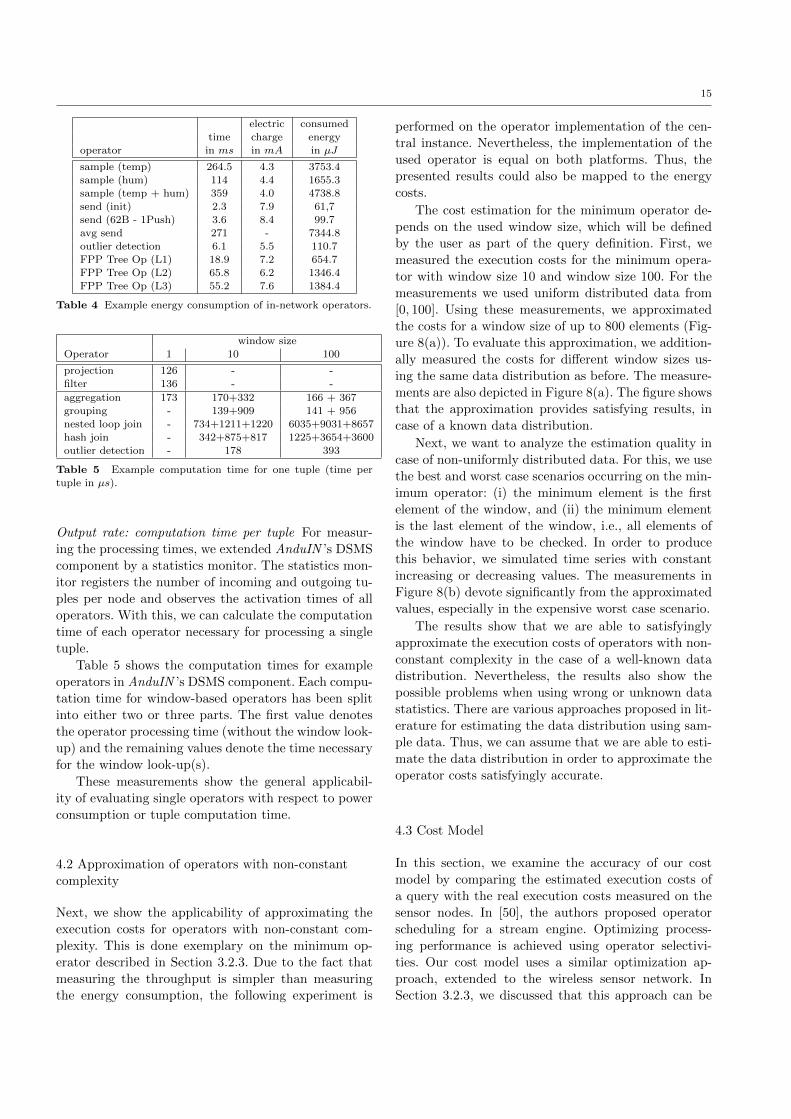
4.2 Approximation of operators with non-constant
complexity
Next, we show the applicability of approximating the
execution costs for operators with non-constant com-
plexity. This is done exemplary on the minimum op-
erator described in Section 3.2.3. Due to the fact that
measuring the throughput is simpler than measuring
the energy consumption, the following experiment is
performed on the operator implementation of the cen-
tral instance. Nevertheless, the implementation of the
used operator is equal on both platforms. Thus, the
presented results could also be mapped to the energy
costs.
The cost estimation for the minimum operator de-
pends on the used window size, which will be defined
by the user as part of the query definition. First, we
measured the execution costs for the minimum opera-
tor with window size 10 and window size 100. For the
measurements we used uniform distributed data from
[0, 100]. Using these measurements, we approximated
the costs for a window size of up to 800 elements (Fig-
ure 8(a)). To evaluate this approximation, we addition-
ally measured the costs for different window sizes us-
ing the same data distribution as before. The measure-
ments are also depicted in Figure 8(a). The figure shows
that the approximation provides satisfying results, in
case of a known data distribution.
Next, we want to analyze the estimation quality in
case of non-uniformly distributed data. For this, we use
the best and worst case scenarios occurring on the min-
imum operator: (i) the minimum element is the first
element of the window, and (ii) the minimum element
is the last element of the window, i.e., all elements of
the window have to be checked. In order to produce
this behavior, we simulated time series with constant
increasing or decreasing values. The measurements in
Figure 8(b) devote significantly from the approximated
values, especially in the expensive worst case scenario.
The results show that we are able to satisfyingly
approximate the execution costs of operators with non-
constant complexity in the case of a well-known data
distribution. Nevertheless, the results also show the
possible problems when using wrong or unknown data
statistics. There are various approaches proposed in lit-
erature for estimating the data distribution using sam-
ple data. Thus, we can assume that we are able to esti-
mate the data distribution in order to approximate the
operator costs satisfyingly accurate.
4.3 Cost Model
In this section, we examine the accuracy of our cost
model by comparing the estimated execution costs of
a query with the real execution costs measured on the
sensor nodes. In [50], the authors proposed operator
scheduling for a stream engine. Optimizing process-
ing performance is achieved using operator selectivi-
ties. Our cost model uses a similar optimization ap-
proach, extended to the wireless sensor network. In
Section 3.2.3, we discussed that this approach can be
16
200
220
240
260
280
300
320
340
0 100 200 300 400 500 600 700 800
measuredapproximated
com
pu
tati
on t
ime
per
tu
ple
window size
(a)
150
200
250
300
350
400
450
500
0 100 200 300 400 500 600 700 800
com
pu
tati
on t
ime
per
tu
ple best−case
approximated
worst−case
window size
(b)
Fig. 8 Estimated and real execution costs for the minimum operator (using different window sizes)
mapped to known fanout-based in-network cost mod-
els. Next, we want to show that the usage of operator
costs and activation frequency is suitable to estimate
the power consumption of the in-network part of An-
duIN queries. For this, we compare the costs computed
by our cost model with the measured real costs.
As one can see from Figure 5 (and which is also re-
flected by the cost model), the overall power consump-
tion is a linear combination of the power consumption
of the different operators. Due to the fact that An-
duIN uses the same runtime environment for each sen-
sor node, it is sufficient to observe a single node’s power
consumption. In the following, we base the comparison
on one query, which is transformed into a set of physical
query plans. The query contains all essential aspects of
a typical in-network query: measuring values, process-
ing these, and sending the results to the base station. In
addition, we use two processing operators with a com-
pletely different power profile.
The comparison is based on the following CQL
query:
SELECT id, time , hum
FROM
(SELECT
id , time , temp ,
hum [outlier (win = >10)]
FROM mystream
) [ dummy ]
Due to the communication protocol of the used Contiki-
like OS and the relatively long transmission times, we
use a sampling interval of two seconds (as sending a
tuple requires up to 532ms, plus the measurement of
the humidity and the execution time of the dummy, an
interval of 1 second could be exceeded).
The inner query in the example performs an out-
lier detection on the attribute hum. In case there are
outliers, the synopsis dummy will be processed and the
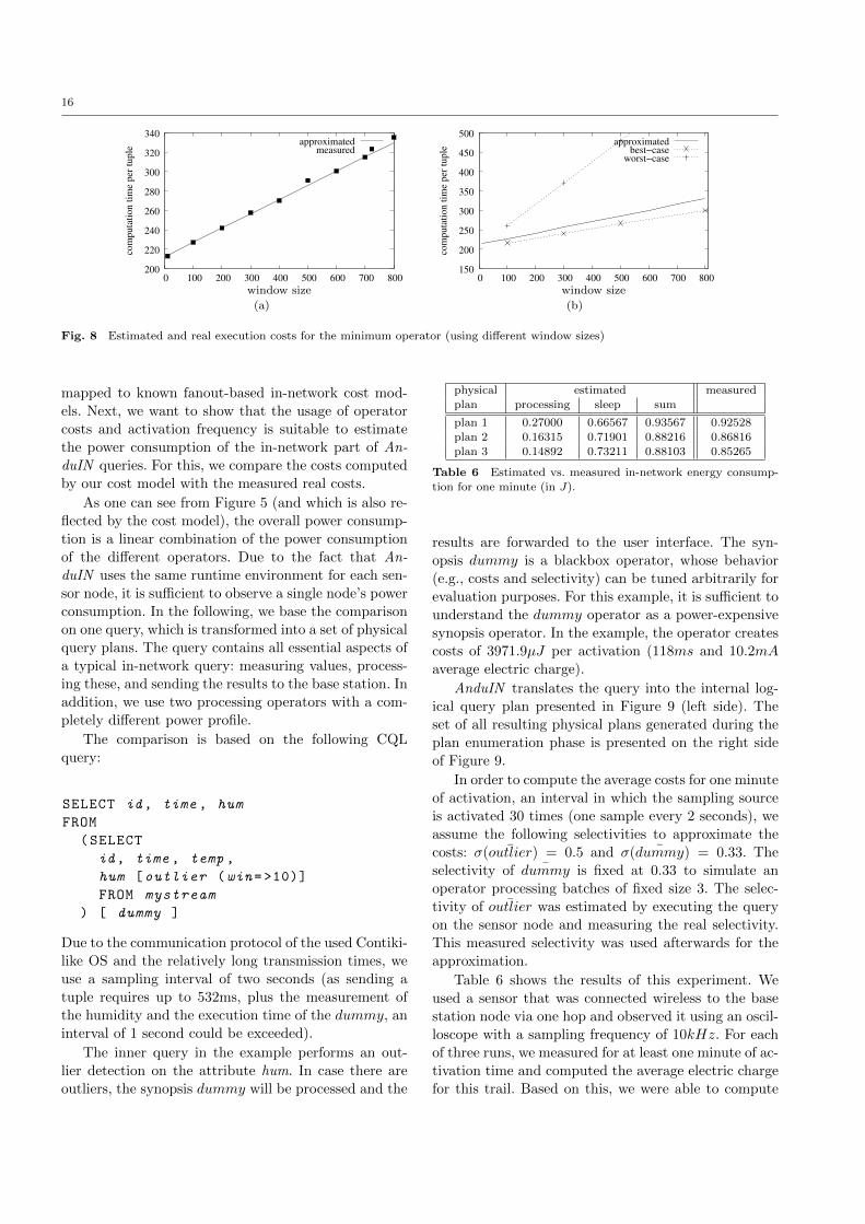
physical estimated measured
plan processing sleep sum
plan 1 0.27000 0.66567 0.93567 0.92528plan 2 0.16315 0.71901 0.88216 0.86816
plan 3 0.14892 0.73211 0.88103 0.85265
Table 6 Estimated vs. measured in-network energy consump-tion for one minute (in J).
results are forwarded to the user interface. The syn-
opsis dummy is a blackbox operator, whose behavior
(e.g., costs and selectivity) can be tuned arbitrarily for
evaluation purposes. For this example, it is sufficient to
understand the dummy operator as a power-expensive
synopsis operator. In the example, the operator creates
costs of 3971.9µJ per activation (118ms and 10.2mA
average electric charge).
AnduIN translates the query into the internal log-
ical query plan presented in Figure 9 (left side). The
set of all resulting physical plans generated during the
plan enumeration phase is presented on the right side
of Figure 9.
In order to compute the average costs for one minute
of activation, an interval in which the sampling source
is activated 30 times (one sample every 2 seconds), we
assume the following selectivities to approximate the
costs: σ( ¯outlier) = 0.5 and σ( ¯dummy) = 0.33. The
selectivity of ¯dummy is fixed at 0.33 to simulate an
operator processing batches of fixed size 3. The selec-
tivity of ¯outlier was estimated by executing the query
on the sensor node and measuring the real selectivity.
This measured selectivity was used afterwards for the
approximation.
Table 6 shows the results of this experiment. We
used a sensor that was connected wireless to the base
station node via one hop and observed it using an oscil-
loscope with a sampling frequency of 10kHz. For each
of three runs, we measured for at least one minute of ac-
tivation time and computed the average electric charge
for this trail. Based on this, we were able to compute
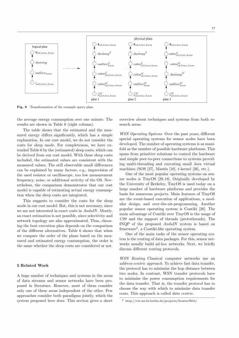
17
logical plan
physical plans
plan 2 plan 3plan 1
ζid,time,hum
outlierhum
zid,time,hum
dummy
¯dummyL
outlierLhum
¯connLid,time,hum
¯connNid,time,hum
ζNid,time,hum
zid,time,hum
ζNid,time,hum
zid,time,hum
¯connNid,time,hum
ζNid,time,hum
zid,time,hum
¯connNid,time,hum
¯connLid,time,hum
outlierNhum outlierNhum
¯dummyL
¯dummyN
¯connLid,time,hum
Fig. 9 Transformation of the example query plan.
the average energy consumption over one minute. The
results are shown in Table 6 (right column).
The table shows that the estimated and the mea-
sured energy differs significantly, which has a simple
explanation. In our cost model, we do not consider the
costs for sleep mode. For completeness, we have ex-
tended Table 6 by the (estimated) sleep costs, which can
be derived from our cost model. With these sleep costs
included, the estimated values are consistent with the
measured values. The still observable small differences
can be explained by many factors, e.g., imprecision of
the used resistor or oscilloscope, too low measurement
frequency, noise, or additional activity of the OS. Nev-
ertheless, the comparison demonstrates that our cost
model is capable of estimating actual energy consump-
tion when the sleep costs are integrated.
This suggests to consider the costs for the sleepmode in our cost model. But, this is not necessary, since
we are not interested in exact costs in AnduIN . Mostly,
an exact estimation is not possible, since selectivity and
network topology are also approximated. Thus, choos-
ing the best execution plan depends on the comparison
of the different alternatives. Table 6 shows that when
we compare the order of the plans based on the mea-
sured and estimated energy consumption, the order is
the same whether the sleep costs are considered or not.
5 Related Work
A huge number of techniques and systems in the areas
of data streams and sensor networks have been pro-
posed in literature. However, most of them consider
only one of these areas independent of the other. Few
approaches consider both paradigms jointly, which the
system proposed here does. This section gives a short
overview about techniques and systems from both re-
search areas.
WSN Operating Systems Over the past years, different
special operating systems for sensor nodes have been
developed. The number of operating systems is as mani-
fold as the number of possible hardware platforms. This
spans from primitive solutions to control the hardware
and simple peer-to-peer connections to systems provid-
ing multi-threading and executing small Java virtual
machines (SOS [27], Mantis [10], t-kernel [26], etc.).
One of the most popular operating systems on sen-
sor nodes is TinyOS [29,18]. Originally developed by
the University of Berkeley, TinyOS is used today on a
large number of hardware platforms and provides the
basis for numerous projects. Main features of TinyOS
are the event-based execution of applications, a mod-
ular design, and over-the-air-programming. Another
popular sensor operating system is Contiki [20]. The
main advantage of Contiki over TinyOS is the usage of
C99 and the support of threads (protothreads). The
INQP of the proposed AnduIN system is based on
feuerware2, a Contiki-like operating system.
One of the main tasks of the sensor operating sys-
tem is the routing of data packages. For this, sensor net-
works usually build ad-hoc networks. Next, we briefly
discuss different routing protocols.
WSN Routing Classical computer networks use an
address-centric approach. To achieve fast data transfer,
the protocol has to minimize the hop distance between
two nodes. In contrast, WSN transfer protocols have
to minimize the power consumption requirements for
the data transfer. That is, the transfer protocol has to
choose the way with which to minimize data transfer
costs. This approach is called data centric.
2 http://cst.mi.fu-berlin.de/projects/ScatterWeb/
18
Communication protocols in WSN can be grouped
into two classes: flat networks and hierarchical networks
[44]. The most popular protocols for flat network struc-
tures are push diffusion [28] and directed diffusion [31].
With hierarchical protocols, the network layer cre-
ates a topology that is used for the complete data trans-
fer. For chained-based aggregation protocols like PEGA-
SIS [36], messages are transferred along a chain built by
nodes with minimal distance. Chained-based protocols
are very efficient (depending on the build algorithm),
but in general they are not robust against node failures.
Tree-based aggregation protocols like TAG (Tiny AG-
gregation) [38] build tree structures. In such a structure,
inner nodes aggregate the data on the path to the tree
root. In cluster-based protocols, nodes inside a neigh-
borhood chose one node within this neighborhood as
the cluster head responsible for data aggregation and
communication with nodes outside the neighborhood.
In general, the cluster head is more heavily used than
other nodes. In order to disseminate these costs over
all nodes within a cluster, solutions like LEACH [41]
regularly change the cluster head.
In general, the used routing strategy is part of the
network layer of the operating system. On WSN, the
operating system and applications like the query layer
on TinyDB are interwoven and inseparable. For in-
stance, Madden et. al introduced in [40] Semantic Rout-
ing Trees (SRT) as part of TinyDB. This is another
routing approach based on query semantics. This means
that a node decides for itself which child nodes receive
queries and which do not. If a sub-tree can contribute
to a query result, the node forwards the query to this
part of the SRT, otherwise the node refuses the query.
Power consumption estimation Due to limited power
resources, energy consumption is the most critical prop-
erty in sensor networks. In order to evaluate topologies,
protocols, and in-network operators, a precise energy
model is essential. Network simulation environments
like PowerTOSSIM [46,42] and SensorSim [45] provide
accurate per-node power consumption analyses. In or-
der to achieve simulations with a high level of accuracy,
real sensors are observed during a benchmarking phase.
For this, the original sensor code has to be extended by
(possibly small) changes necessary for measuring the
energy consumption. Afterwards, the simulation envi-
ronment is able to use the real power consumptions to
approximate the costs for different topologies and prop-
agation strategies.
Different analytical cost models [15,16] have been
proposed in literature. They are often designed inde-
pendently of the used physical network layer and geared
towards predicting the residual lifetime of the sensor
network. The cost model presented in [51] was designed
to compute the benefits of a (partial) merge of queries
(in context of multi-query optimization for sensor net-
works). The authors also considered the selectivity of
predicates to estimate the power consumption for a sin-
gle query.
As discussed before, for AnduIN it is not important
to compute the real power consumption of sensor nodes.
For instance, costs for maintaining routing structures
will be independent of running queries. Of course, they
are essential for the sensor network itself, but not for
the comparison of different query workloads. Because
of this, AnduIN follows the analytical cost model.
INQP One of the first systems including sensor nodes
into query computation was Fjords (Framework in Java
for Operators on Remote Data Streams) [39]. Opposed
to later systems, Fjords was not designed for in-network
query processing. Thus, sensor nodes only measure val-
ues. Results are sent to proxy servers, which serve as
caches and simple filters. Afterwards, the proxy servers
send their results to the target server. In addition to
the primitive pre-processing, the proxy servers have the
opportunity to adapt the sensor nodes’ sampling times
and can pull measurements from them.
The Cougar project [53,52] was one of the first
projects to bring database concepts into the world of
sensor networks. For this, each sensor node was ex-
panded by a query layer, which serves as a layer between
the user application and the sensor network. Cougar
differentiates between three classes of sensor nodes: (i)
source nodes, (ii) inner nodes, and (iii) the gate node.
Source nodes only measure values, inner nodes addi-
tionally compute some simple operations, and the gate
node serves as a connection to other sinks and provides
a simple query optimizer. First in-network aggregation
approaches were introduced along with Cougar, such as
packet merging and partial aggregation [52].
One of the most well known INQP is TinyDB, first
presented by Madden et. al [37,40]. Since all values
produced by TinyDB are stored within a virtual Ta-
ble sensor, TinyDB is called a declarative database
systems for sensor networks. Each row of sensor rep-
resents the state of one node at one time, while columns
represent the attributes. In the context of TinyDB,
Madden et. al also introduced ACQP, a special query
language adapted to the requirements of sensor net-
works. Due to the monolithic design of TinyDB, a large
number of operations is integrated. The most popular
operators are acquisition, filter, projection, aggregation,
grouping, and join operators. The limited memory re-
sources results in the lack of alternative, more power-
19
efficient implementations of the join operator: by de-
fault, TinyDB supports only the nested-loop join.
DSMS Opposed to in-network processors, central data
stream processors often support the processing of a
huge number of operators including complex mining al-
gorithms. One of the first systems particularly devel-
oped for data stream processing was STREAM (Stan-
ford Stream Data Manager) [5,4], where data flows
from sources to sinks. One of the fundamental concepts
of STREAM is its translation between data streams
and relations. Streams are mapped into relations using
a stream-to-relation operator. Subsequently, the rela-
tion can be processed using known database utilities.
After the in-relation processing, the relations must be
translated back into streams using a relation-to-stream
operator.
Together with STREAM, the query language CQL
(Continuous Query Language) was introduced [6,4,7].
CQL is based on the SQL standard extended by a syn-
opses operator and the relation-to-stream operators.
The query language used in AnduIN is based on CQL,
but AnduIN does not use the relation-to-stream oper-
ators, since it works directly on streams.
The TelegraphCQ project [14,13] uses a different
data-stream approach. In TelegraphCQ, tuples flow
through operators controlled by modules called Eddies
[8]. Each tuple holds a bitmap, containing a list of op-
erators that it has already visited. Based on this, the
Eddies decide which operator is the next to process the
tuple.
Combined DSMS/INQP There are few approaches
that try to combine DSMS with INQP. For instance,
the Borealis Project [1,3] focuses on distributed data
stream processing, where each distributed node works
as a data stream server. Using a proxy-server approach
(similar to Fjords), Borealis is also able to integrate
WSN into the stream processing. The main problem of
this approach is that the system considers the whole
WSN as one operator. A DSMS/INQP overlapping op-
timization like that in AnduIN is not intended. An-
other combined DSMS/INQP is the HiFi project [17].
HiFi is a combination of TelegraphCQ and TinyDB,
where TinyDB is considered as a black box. Neverthe-
less, the usage of TinyDB results in the same problems
that TinyDB has itself. The monolithic approach sup-
ports only a restricted number of operators.
An approach similar to AnduIN was proposed
in [19]. The authors also developed a system that builds
the sensor nodes’ runtime environment based on the set
of running queries. In contrast, AnduIN integrates this
approach into an existing data stream engine and pro-
vides complex operators like frequent pattern mining
and burst detection.
6 Conclusion and Outlook
In this paper, we presented AnduIN , a system support-
ing partial in-network query processing in wireless sen-
sor networks. AnduIN is composed of two components,
a central DSMS and a distributed INQP. We introduced
a new approach to handling complex operators, and,
based on this, we developed and evaluated a cost model
for approximating energy consumption.
In its current state, AnduIN supports a very large
number of operators in both the central and the in-
network component. Nevertheless, most of the synopses
operators are only a part of the central instance, and
future work includes an analysis of options to imple-
ment them (partially) as in-network operators. At the
moment, AnduIN deploys queries only once – at the
query generation time. In general, data and network
characteristics can change over time, especially in dy-
namic environments. Then, the optimal execution plan
can change and should ideally supplant an outdated
running plan. Therefore, the exchange of sensor nodes’
images is part of our future work, along with the de-
velopment of multi-query optimization (MQO). All this
will be the focus of a self-contained work on adaptive
query planning and processing. In AnduIN , operators
can be integrated multiple times into the same node’s
image and execution plans can contain redundant oper-
ations, wasting limited memory and energy resources.
Thus, the reuse of operators is a promising direction.
Future work on AnduIN is especially promising due to
its modular design, which supports simple integration
of new optimization techniques.
References
1. D. J. Abadi, Y. Ahmad, M. Balazinska, M. Cherniack,
J. h. Hwang, W. Lindner, A. S. Maskey, E. Rasin, E. Ryvk-ina, N. Tatbul, Y. Xing, and St. Zdonik. The design of the
borealis stream processing engine. In CIDR, pages 277–289,
2005.
2. Ch. C. Aggarwal, J. Han, J. Wang, and Ph. S. Yu. A Frame-work for Clustering Evolving Data Streams. In VLDB, pages
81–92, 2003.
3. Y. Ahmad, A. Jhingran, B. Berg, A. Maskey, W. Xing, O. Pa-
paemmanouil, Y. Xing, M. Humphrey, A. Rasin, and St.
Zdonik. Distributed operation in the borealis stream pro-cessing engine. In SIGMOD, 2005.
4. A. Arasu, B. Babcock, Sh. Babu, J. Cieslewicz, K. Ito,
R. Motwani, U. Srivastava, and J. Widom. Stream: Thestanford data stream management system. Springer, 2004.
20
5. A. Arasu, B. Babcock, Sh. Babu, M. Datar, K. Ito,I. Nishizawa, J. Rosenstein, and J. Widom. Stream: the stan-
ford stream data manager (demonstration description). In
SIGMOD, pages 665–665, New York, NY, USA, 2003. ACM.6. A. Arasu, Sh. Babu, and J. Widom. The CQL Continuous
Query Language: Semantic Foundations and Query Execu-
tion. Technical report, University of Stanford, 2003.7. A. Arasu, Sh. Babu, and J. Widom. The cql continuous
query language: semantic foundations and query execution.
The VLDB Journal, 15(2):121–142, 2006.8. R. Avnur and J. Hellerstein. Eddies: Continuously Adaptive
Query Processing. In SIGMOD, pages 261–272, 2000.9. B. Babcock, M. Datar, and R. Motwani. Load shedding tech-
niques for data stream systems. In MPDS 2003, 2003.10. Sh. Bhatti, J. Carlson, H. Dai, J. Deng, J. Rose, A. Sheth,
B. Shucker, Ch. Gruenwald, A. Torgerson, and R. Han. Man-
tis os: an embedded multithreaded operating system for wire-less micro sensor platforms. Mobile Network Applications,
10(4):563–579, 2005.11. S. Borzsonyi, D. Kossmann, and K. Stocker. The skyline
operator. In ICDE’01, pages 421–432, 2001.12. D. Carney, U. Centintemel, A. Rasin, S. B. Zdonik, M. Cher-
niack, and M. Stonebraker. Monitoring streams: A new classof data management applications. In VLDB, pages 215–226.
VLDB Endowment, 2002.13. S. Chandrasekaran, O. Cooper, A. Deshpande, M. Franklin,
J. Hellerstein, W. Hong, S. Krishnamurthy, S. Madden,
V. Raman, F. Reiss, and M. Shah. TelegraphCQ: Contin-
uous Dataflow Processing for an Uncertain World. In CIDR,2003.
14. S. Chandrasekaran, O. Cooper, A. Deshpande, M. J.
Franklin, J. M. Hellerstein, W. Hong, S. Krishnamurthy, S. R.Madden, F. Reiss, and M. A. Shah. Telegraphcq: continuous
dataflow processing. In SIGMOD, pages 668–668, New York,
NY, USA, 2003. ACM.15. Y. Chen and Q. Zhao. On the lifetime of wireless sensor
networks. IEEE Commun. Lett, 9:976–978, 2004.16. Z. Cheng, M. Perillo, and W. B. Heinzelman. General net-
work lifetime and cost models for evaluating sensor network
deployment strategies. IEEE Transactions on Mobile Com-
puting, 2008.17. O. Cooper, A. Edakkunni, M. Franklin, W. Hong, S. Jeffery,
S. Krishnamurthy, F. Reiss, S. Rizvi, and E. Wu. HiFi: A
unified architecture for high fan-in systems. In VLDB, pages1357–1360. Demo, 2004.
18. D. E. Culler, J. Hill, P. Buonadonna, R. Szewczyk, and
A. Woo. A network-centric approach to embedded soft-
ware for tiny devices. Lecture Notes in Computer Science,2211:114–130, 2001.
19. F. Dressler, R. Kapitza, M. Daum, M. Strube, W. Schroder-
Preikschat, R. German, and Kl. Meyer-Wegener. Query pro-cessing and system-level support for runtime-adaptive sensor
networks. In KiVS, pages 55–66, 2009.20. A. Dunkels, B. Groenvall, and Th. Voigt. Contiki - a
lightweight and flexible operating system for tiny networked
sensors. In LCN, pages 455–462, 2004.21. T. Rossbach E. Chervakova, D. Klan. Energy-optimized sen-
sor data processing. In EUROSSC, pages 35–38, 2009.22. C. Franke, M. Hartung, M. Karnstedt, and K. Sattler.
Quality-Aware Mining of Data Streams. In IQ, pages 300–315, 2005.
23. C. Franke, M. Karnstedt, D. Klan, M. Gertz, K.-U. Sattler,
and W. Kattanek. In-network detection of anomaly regionsin sensor networks with obstacles. In BTW, pages 367–386,
2009.24. C. Giannella, J. Han, E. Robertson, and C. Liu. Mining
Frequent Itemsets over Arbitrary Time Intervals in DataStreams. Technical report, Indiana University, 2003.
25. P. Godfrey, R. Shipley, and J. Gryz. Algorithms and anal-yses for maximal vector computation. The VLDB Journal,
16(1):5–28, 2007.26. L. Gu and J. A. Stankovic. t-kernel: providing reliable os
support to wireless sensor networks. In Sensys ’06, pages1–14, New York, NY, USA, 2006. ACM.
27. Ch.-Ch. Han, R. Kumar, R. Shea, E. Kohler, and M. Sri-
vastava. A dynamic operating system for sensor nodes. In
Mobisys, pages 163–176, New York, NY, USA, 2005. ACM.28. W. R. Heinzelman, J. Kulik, and H. Balakrishnan. Adap-
tive protocols for information dissemination in wireless sen-
sor networks. In Mobicom, pages 174–185, New York, NY,
USA, 1999. ACM.29. J. Hill, R. Szewczyk, A. Woo, S. Hollar, D. Culler, and K. Pis-
ter. System architecture directions for networked sensors. In
In Architectural Support for Programming Languages and
Operating Systems, pages 93–104, 2000.30. Th. Hillebrandt. Diploma-thesis: Untersuchung und simu-
lation des zeit- und energie- verhaltens eines msb430-h sen-
sornetzwerkes. Department of Mathematics and ComputerScience, FU Berlin, 2007.
31. C. Intanagonwiwat, R. Govindan, and D. Estrin. Directed
diffusion: a scalable and robust communication paradigm for
sensor networks. In Mobicom, pages 56–67, New York, NY,USA, 2000. ACM.
32. M. Karnstedt, D. Klan, Chr. Politz, K.-U. Sattler, and
C. Franke. Adaptive burst detection in a stream engine. In
SAC, pages 1511–1515, New York, NY, USA, 2009. ACM.33. D. Klan, K. Hose, M. Karnstedt, and K. Sattler. Power-
Aware Data Analysis in Sensor Networks. In ICDE 2010,
pages 1125–1128, 2010.34. J. Kramer and B. Seeger. PIPES - A Public Infrastructure
for Processing and Exploring Streams. In SIGMOD, pages925–926, 2004.
35. S. Lindsey and C. Raghavendra. Pegasis: Power-efficient
gathering in sensor information systems. Aerospace Con-
ference Proceedings, 2002. IEEE, 3:1125–1130, 2002.36. St. Lindsey, C. Raghavendra, and K. M. Sivalingam. Data
gathering algorithms in sensor networks using energy met-
rics. IEEE Trans. Parallel Distrib. Syst., 13(9):924–935,
2002.37. S. Madden. The design and evaluation of a query processing
architecture for sensor networks. Technical report, 2003.38. S. Madden, M. Franklin, J. Hellerstein, and W. Hong. TAG:
a Tiny AGgregation service for ad-hoc sensor networks.
SIGOPS Oper. Syst. Rev., 36(SI):131–146, 2002.39. S. Madden and M.J. Franklin. Fjording the stream: An ar-
chitecture for queries over streaming sensor data, 2002.40. S .R. Madden, M. J. Franklin, J. M. Hellerstein, and
W. Hong. TinyDB: an acquisitional query processing sys-tem for sensor networks. ACM Trans. on Database Systems,
30(1):122–173, 2005.41. P. Chandrakasan and W.B. Heinzelman. Application-specific
protocol architectures for wireless networks. IEEE Transac-tions on Wireless Communications, 1:660–670, 2000.
42. Enrico Perla, Art O Cathain, Ricardo Simon Carbajo, MerielHuggard, and Ciaran Mc Goldrick. Powertossim z: realistic
energy modelling for wireless sensor network environments.In PM2HW2N, pages 35–42. ACM, 2008.
43. F. P. Preparata and M. I. Shamos. Computational Geometry
- An Introduction. Springer, 1985.44. R. Rajagopalan and P. K. Varshney. Data aggregation tech-
niques in sensor networks: A survey. Comm. Surveys & Tu-torials, IEEE, 8:48–63, 2006.
45. S. Park, A. Savvides, and M. B. Srivastava. Sensorsim: a sim-
ulation framework for sensor networks. In Modeling, Anal-
ysis and Simulation of Wireless and Mobile Systems, pages104–111, Boston, MA USA, 2000.
21
46. V. Shnayder, M. Hempstead, B. Chen, G.W. Allen, andM. Welsh. Simulating the power consumption of large-scale
sensor network applications. In Sensys, pages 188–200. ACM
Press, 2004.
47. K. Sohrabi, J. Gao, V. Ailawadhi, and G. J. Pottie. Proto-
cols for self-organization of a wireless sensor network. IEEEPersonal Communications, 7:16–27, 2000.
48. J. D. Ullman, H. Garcia-Molina, and J. Widom. Database
Systems: The Complete Book. Prentice Hall PTR, UpperSaddle River, NJ, USA, 2001.
49. St. D. Viglas and J. F. Naughton. Rate-based query opti-
mization for streaming information sources. In SIGMOD,pages 37–48, New York, NY, USA, 2002. ACM.
50. J. Widom and R. Motwani. Query processing, resource man-
agement, and approximation in a data stream managementsystem. In CIDR, pages 245–256, 2003.
51. Sh. Xiang, H. B. Lim, and K.-L. Tan. Impact of multi-query
optimization in sensor networks. In DMSN, pages 7–12, 2006.
52. Y. Yao and J. Gehrke. Query processing in sensor networks.
CIDR, January 2003.
53. Y. Yao and J. E. Gehrke. The cougar approach to in-networkquery processing in sensor networks. ACM SIGMOD Record,
31(2):9–18, 2002.
Daniel Klan is a Ph.D. stu-
dent at the Database & Informa-tion Systems group at the Fac-
ulty of Computer Science andAutomation of the Ilmenau Uni-
versity of Technology, Germany.
He received his Diploma (M.Sc.)in Computer Science from the
University of Jena, Germany.
His current research interestsinclude data mining on data
streams and sensor networks.
Marcel Karnstedt received
his Diploma (M.Sc.) in 2003
from the Martin-Luther-Universitat Halle-Wittenberg,
Germany. He successfully fin-
ished his Ph.D. in 2009 atthe Databases & InformationSystems Group at the Ilmenau
University of Technology, Ger-many. Since March 2009 he has
been working as a postdoc atDERI, National University of
Ireland, Galway. His researchinterests are on large-scale datamanagement, query processing,
and data mining. His academic
record lists more than 50 publi-
cations in specific areas like P2P databases, stream and graphmining, and distributed query processing. More information can
be found at http://www.marcel.karnstedt.com.
Katja Hose is a postdoc-toral researcher at the Max-
Planck Institute for Informaticsin Saarburcken, Germany. She
received her Diploma (M.Sc.) in
Computer Science from IlmenauUniversity of Technology in 2004
and joined the Databases & In-
formation Systems Group at Il-menau University of Technology
as a research associate. She re-
ceived her doctoral degree inComputer Science in 2009 and
joined the Max-Planck-Institut
fur Informatik in Saarbrucken
in the same year. Her current
research interests range fromquery processing in sensor networks and distributed systems to
Linked Data processing, information retrieval, and knowledge ex-
traction.
Liz Ribe-Baumann is a Ph.D.student with the International
Graduate School on Mobile
Communication at the IlmenauUniversity of Technology, Ger-
many where she belongs to the
Database & Information Sys-tems group of the Faculty of
Computer Science and Automa-tion. She received her Diploma
(M.Sc.) in Mathematics in 2009
from the same university. Hercurrent research interests in-
clude location and resource
aware P2P databases, partic-
ularly from a graph-theoreticpoint of view.
Kai-Uwe Sattler is full pro-
fessor and heads the Database
and Information Systems groupat the Faculty of Computer Sci-
ence and Automation of the Il-
menau University of Technol-ogy, Germany. He received hisDiploma (M.Sc.) in Computer
Science from the University ofMagdeburg, Germany. He re-
ceived his Ph.D. in ComputerScience in 1998 and his Habilita-
tion (venia legendi) in ComputerScience in 2003 from the sameuniversity. He has published five
textbooks and more than 100 re-
search papers. His current re-
search interests include autonomic features in database systemsand large-scale distributed data management.