Structural Macroeconometrics

Chapter 3. Removing Trends and Isolating Cycles

David N. DeJong Chetan Dave

Just as DSGE models must be primed for empirical analysis, so too must the corre-

sponding data. Broadly speaking, data preparation involves three steps. A guiding principle

behind all three involves the symmetric treatment of the actual data and their theoretical

counterparts. First, correspondence must be established between what is being characterized

by the model and what is being measured in the data. For example, if the focus is on a

business cycle model that does not include a government sector, it would not be appropriate

to align the model�s characterization of output with the measure of aggregate GDP reported

in the National Income and Product Accounts. The collection of papers in Cooley (1995)

pay careful attention to this issue, and do so for a broad range of models.

The second and third steps involve the removal of trends and the isolation of cycles.

Regarding the former, model solutions are in terms of stationary versions of variables: the

stochastic behavior of the variables is in the form of temporary departures from steady

state values. Corresponding data are represented analogously. So again using a business

cycle model as an example, if the model is designed to characterize the cyclical behavior

of a set of time series, and the time series exhibit both trends and cycles, the trends are

eliminated prior to analysis. In such cases, it is often useful to build both trend and cyclical

behavior into the model, and eliminate trends from the model and actual data in parallel

fashion. Indeed, a typical objective in the business cycle literature is to determine whether

models capable of capturing salient features of economic growth can also account for observed

patterns of business cycle activity. Under this objective, the speci�cation of the model is

subject to the constraint that it must successfully characterize trend behavior. Having

satis�ed the constraint, trends are eliminated appropriately and the analysis proceeds with

an investigation of cyclical behavior. Steady states in this case are interpretable as the

1

relative heights of trend lines.

Regarding the isolation of cycles, this is closely related to the removal of trends. Indeed,

for a time series exhibiting cyclical deviations about a trend, the identi�cation of the trend

automatically serves to identify the cyclical deviations as well. However, even after the

separation of trend from cycle is accomplished, additional steps may be necessary to isolate

cycles by the frequency of their recurrence. Return again to the example of a business cycle

model. By design, the model is intended to characterize patterns of �uctuations in the data

that recur at business cycle frequencies: between approximately six and 40 quarters. It is

not intended to characterize seasonal �uctuations. Yet unless additional steps are taken,

the removal of the trend will leave such �uctuations intact, and their presence can have a

detrimental impact on inferences involving business cycle behavior.1

The isolation of cycles is also related to the task of aligning models with appropriate

data, because the frequency with which data are measured in part determines their cyclical

characteristics. For example, empirical analyses of economic growth typically involve mea-

surements of variables averaged over long time spans (e.g., over half-decade intervals). This

is because the models in question are not designed to characterize business cycle activity,

and time aggregation at the �ve-year level is typically su¢ cient to eliminate the in�uence

of cyclical variations while retaining relevant information regarding long-term growth. For

related reasons, analyses of aggregate asset-pricing behavior are typically conducted using

annual data, which mitigates the need to control, e.g., for seasonal �uctuations. Analyses

of business cycle behavior are typically conducted using quarterly data. Measurement at

1For an example of a model designed to jointly characterize both cyclical and seasonal variations inaggregate economic activity, see Wen (2002).

2

this frequency is not ideal, since it introduces the in�uence of seasonal �uctuations into the

analysis; but on the other hand, aggregation to an annual frequency would entail an impor-

tant loss of information regarding �uctuations observed at business cycle frequencies. Thus

an alternative to time aggregation is needed to isolate cycles in this case.

This chapter presents alternative approaches available for eliminating trends and isolating

cycles. Supplements to the brief coverage of these topics provided here are available from

any number of texts devoted to time series analysis (e.g., Harvey, 1993; Hamilton, 1994).

Speci�c coverage of cycle isolation in the context of business cycle analysis is provided by

Kaiser and Maravall (2001).

To illustrate the concepts introduced in this chapter, we work with a prototypical data

set used to analyze business cycle behavior. It is designed for alignment with the real

business cycle model introduced in Chapter 5. The data are described in full in the appendix,

and are contained in the text �le rbcdata.txt, available for downloading at the textbook

website. Brie�y, the data set consists of four time series: consumption of non-durables and

services; gross private domestic investment; output, measured as the sum of consumption

and investment; and hours of labor supplied in the non-farm business sector. Each variable

is real, measured in per capita terms, and is seasonally adjusted. The data are quarterly,

and span 1948:I through 2004:IV. In addition, we also work with the non-seasonally-adjusted

counterpart to consumption. Logged time series trajectories of the seasonally adjusted data

are illustrated in Figure 3.1.

3

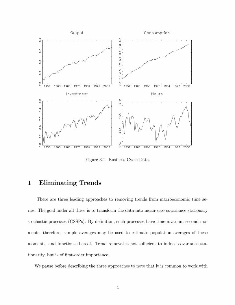
Figure 3.1. Business Cycle Data.

1 Eliminating Trends

There are three leading approaches to removing trends from macroeconomic time se-

ries. The goal under all three is to transform the data into mean-zero covariance stationary

stochastic processes (CSSPs). By de�nition, such processes have time-invariant second mo-

ments; therefore, sample averages may be used to estimate population averages of these

moments, and functions thereof. Trend removal is not su¢ cient to induce covariance sta-

tionarity, but is of �rst-order importance.

We pause before describing the three approaches to note that it is common to work with

4

logged versions of data represented in levels (e.g., as in Figure 3.1). This is because changes

in the log of a variable yt over time represent the growth rate of the variable:

@

@tlog yt =

@@tyt

yt�

�ytyt� gyt ; (1)

where�yt =

@@tyt. In addition, when using log-linear approximations to represent the cor-

responding structural model, working with logged versions of levels of the data provides

symmetric treatment of both sets of variables.

The �rst two approaches to trend removal, detrending and di¤erencing, are conducted un-

der the implicit assumption that the data follow roughly constant growth rates. Detrending

proceeds under the assumption that the level of yt obeys

yt = y0(1 + gy)teut ; ut � CSSP: (2)

Then taking logs,

log yt = log y0 + gyt+ ut; (3)

where log(1 + gy) is approximated as gy. Trend removal is accomplished by �tting a lin-

ear trend to log yt using an ordinary least squares (OLS) regression, and subtracting the

estimated trend:

eyt = log yt �c�0 �c�1 � t = but; (4)

where the b�0s are coe¢ cient estimates. In this case, log yt is said to be trend stationary.In working with a set ofm variables characterized by the corresponding model as sharing a

5

common trend component (i.e., exhibiting balanced growth), symmetry dictates the removal

of a common trend from all variables. De�ning �j1 as the trend coe¢ cient associated with

variable j, this is accomplished via the imposition of the linear restrictions

�11 � �j1 = 0; j = 2; :::;m;

easily imposed in an OLS estimation framework.2

Di¤erencing proceeds under the assumption that yt obeys

yt = y0e"t ; (5)

"t = + "t�1 + ut; ut � CSSP: (6)

Note from (6) that iterative substitution for "t�1; "t�2; :::, yields an expression for "t of the

form

"t = � t+t�1Xj=0

ut�j + "0; (7)

and thus the growth rate of yt is given by . From (5),

log yt = log y0 + "t: (8)

Thus the �rst di¤erence of log yt, given by log yt � log yt�1 � (1 � L) log yt, where the lag

2The GAUSS procedure ct.prc, available at the textbook website, serves this purpose.

6

operator L is de�ned such that Lpyt = yt�p, is stationary:

log yt � log yt�1 = "t � "t�1 (9)

= + ut:

In this case, log yt is said to be di¤erence stationary. Estimating using the sample average

of log yt � log yt�1 yields the desired transformation of yt:

eyt = log yt � log yt�1 � b = but: (10)

Once again, a common growth rate may be imposed across a set of variables via restricted

OLS by estimating b j subject to the restrictionb 1 � b j = 0; j = 2; :::;m; (11)

ct.prc is also available for this purpose.

The choice between detrending versus di¤erencing hinges on assumptions regarding whether

(3) or (9) provides a more appropriate representation for log yt. Nelson and Plosser (1982)

initiated an intense debate regarding this issue, and despite the large literature that followed,

the issue has proven di¢ cult to resolve.3 A remedy for this di¢ culty is to work with both

speci�cations in turn, and evaluate the sensitivity of results on the chosen speci�cation.

As Figure 3.2 illustrates, the choice of either speci�cation is problematic in the present em-

3For an overview of this literature, see, e.g., DeJong and Whiteman (1993) and Stock (1994).

7

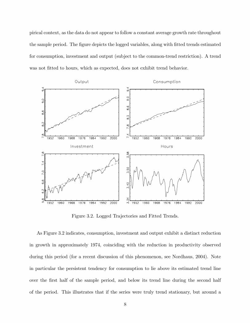
pirical context, as the data do not appear to follow a constant average growth rate throughout

the sample period. The �gure depicts the logged variables, along with �tted trends estimated

for consumption, investment and output (subject to the common-trend restriction). A trend

was not �tted to hours, which as expected, does not exhibit trend behavior.

Figure 3.2. Logged Trajectories and Fitted Trends.

As Figure 3.2 indicates, consumption, investment and output exhibit a distinct reduction

in growth in approximately 1974, coinciding with the reduction in productivity observed

during this period (for a recent discussion of this phenomenon, see Nordhaus, 2004). Note

in particular the persistent tendency for consumption to lie above its estimated trend line

over the �rst half of the sample period, and below its trend line during the second half

of the period. This illustrates that if the series were truly trend stationary, but around a

8

broken trend line, the detrended series will exhibit a spurious degree of persistence, tainting

inferences regarding their cyclical behavior (see Perron, 1989 for a discussion of this issue).

Likewise, the removal of a constant from �rst di¤erences of the data will result in series

that persistently lie above and below zero, also threatening to taint inferences regarding

cyclicality.

The third approach to detrending involves the use of �lters designed to separate trend

from cycle, but given the admission of a slowly evolving trend. In this section we introduce

the Hodrick-Prescott (H-P) �lter, which has proven popular in business cycle applications.

In Section 3.2, we introduce a leading alternative to the H-P �lter: band pass �lters.

Decomposing log yt as

log yt = gt + ct; (12)

where gt denotes the growth component of log yt and ct denotes the cyclical component, the

H-P �lter estimates gt and ct in order to minimize

TXt=1

c2t + �TXt=3

�(1� L)2 gt

�2; (13)

taking � as given.4 Trend removal is accomplished simply as

eyt = log yt � bgt = bct: (14)

The parameter � in (13) determines the importance of having a smoothly evolving growth

component: the smoother is gt, the smaller will be its second di¤erence. With � = 0, smooth-

4The GAUSS procedure hpfilter.prc is available for this purpose.

9

ness receives no value, and all variation in log yt will be assigned to the trend component.

With �!1, the trend is assigned to be maximally smooth, i.e., linear.

In general, � is speci�ed to strike a compromise between these two extremes. In working

with business cycle data, the standard choice is � = 1; 600. To explain the logic behind this

choice and what it accomplishes, it is necessary to venture into the frequency domain. Before

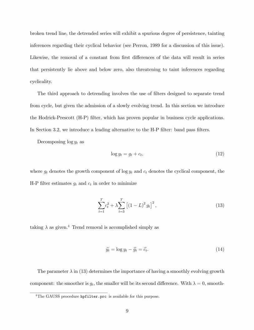
doing so, we illustrate the trajectories of bgt resulting from this speci�cation for the example

data, including hours.5 These are presented in Figure 3.3. The evolution of the estimated bgt�sserves to underscore the mid-1970s reduction in the growth rates of consumption, investment

and output discussed above.

Figure 3.3. Logged Trajectories and H-P Trends.

5In business cycle applications, it is conventional to apply the H-P �lter to all series, absent a common-trend restriction.

10

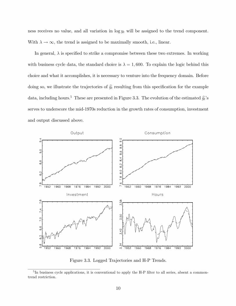
The versions of detrended output eyt generated by these three trend-removal proceduresare illustrated in Figure 3.4. Most striking is the di¤erence in volatility observed across the

three measures: the standard deviation of the linearly detrended series is 0.046, compared

with 0.010 for the di¤erenced series and 0.018 for the H-P �ltered series. The behavior of

the linearly detrended series is dominated by the large and extended departure above zero

during the mid-1960s through the mid-1970s, and the subsequent reversal at the end of the

sample. This behavior provides an additional indication of the trend break observed for

this series in the mid-1970s. The correlation between the linearly detrended and di¤erenced

series is only 0.12; the correlation between the linearly detrended and H-P �ltered series is

0.49; and the correlation between the H-P �ltered and di¤erenced series is 0.27.

Figure 3.4. Detrended Output. {Lin. Det.: solid; Di¤�ed: Dots; H-P Filtered: Dashes}

11

2 Isolating Cycles

Consider the behavior of a time series y!t given by

y!t = �(!) cos(!t) + �(!) sin(!t); (15)

where �(!) and �(!) are uncorrelated zero-mean random variables with equal variances. The

parameter !, measured in radians, determines the frequency with which cos(!t) completes

a cycle relative to cos(t) as t evolves from 0 to 2�, 2� to 4�, etc. (the frequency for cos(t)

being 1). The upper panels of Figure 3.5 depict cos(!t) and sin(!t) as t evolves from 0 to

2� for ! = 1 and ! = 2. Accordingly, given realizations for �(!) and �(!), y!t follows a

deterministic cycle that is completed ! times as t ranges from 0 to 2�, etc. This is depicted

in the lower panels of Figure 3.5, using �(!) = �(!) = 1, ! = 1 and ! = 2.

12

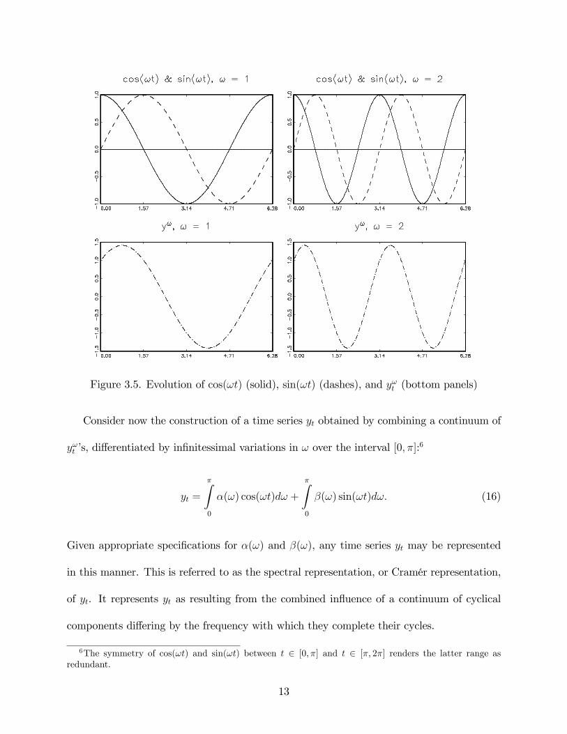
Figure 3.5. Evolution of cos(!t) (solid), sin(!t) (dashes), and y!t (bottom panels)

Consider now the construction of a time series yt obtained by combining a continuum of

y!t �s, di¤erentiated by in�nitessimal variations in ! over the interval [0; �]:6

yt =

�Z0

�(!) cos(!t)d! +

�Z0

�(!) sin(!t)d!: (16)

Given appropriate speci�cations for �(!) and �(!), any time series yt may be represented

in this manner. This is referred to as the spectral representation, or Cramér representation,

of yt. It represents yt as resulting from the combined in�uence of a continuum of cyclical

components di¤ering by the frequency with which they complete their cycles.

6The symmetry of cos(!t) and sin(!t) between t 2 [0; �] and t 2 [�; 2�] renders the latter range asredundant.

13

Closely related to the spectral representation of yt is its power spectrum, or spectrum.

This is a tool that measures the contribution to the overall variance of yt made by the cyclical

components y!t over the continuum [0; �]. Speci�cally, the spectrum is a decomposition of the

variance of yt by frequency. The foundation of the spectrum is the autocovariance function

of yt. Letting (�) denote the autocovariance between yt and yt+� (or equivalently, between

yt and yt�� ), with (0) denoting the variance of yt, the autocovariance function is simply a

plot of (�) against � . Having de�ned the autocovariance function, the spectrum of yt is

given by

sy(!) =

�1

2�

�" (0) + 2

1X�=1

(�) cos(!�)

#: (17)

The integral of sy(!) over the range [��; �] yields (0), and comparisons of the height of

sy(!) for alternative values of ! indicate the relative importance of �uctuations at the chosen

frequencies in in�uencing variations in yt. Since cos(!�) is symmetric over [��; 0] and [0; �],

so too is s(!); it is customary to represent sy(!) over [0; �].

To obtain an interpretation for frequency in terms of units of time rather than radians,

it is useful to relate ! to its associated period p, de�ned as the number of units of time

necessary for y!t to complete a cycle: p = 2�=!. In turn, 1=p = !=2� indicates the number

of cycles completed by y!t per period. For example, with a period representing a quarter, a

ten-year or 40-quarter cycle has an associated value of ! of 2�=40 = 0:157. For a 6-quarter

cycle, ! = 2�=6 = 1:047. Thus values for ! in the range [0:157; 1:047] are of central interest

in analyzing business cycle behavior.

Returning to the problem of trend removal, it is useful to think of a slowly evolving

trend as a cycle with very low frequency; in the case of a constant trend, the associated

14

frequency is zero. Filters are tools designed to eliminate the in�uence of cyclical variation

at various frequencies. Detrending �lters such as the �rst-di¤erence and H-P �lters target

low frequencies; seasonal �lters target seasonal frequencies; etc. The general form of a linear

�lter applied to yt, producing yft , is given by

yft =sX

j=�rcjyt�j � C(L)yt: (18)

In the frequency domain, the counterpart to C(L) is obtained by replacing Lj with e�i!j =

cos(!j) � i sin(!j), wherepi = �1; i.e., i is imaginary. This replacement is known as a

Fourier transformation. The result is the frequency response function: C(e�i!).

With the introduction of an additional tool, we can describe how �lters are used to

manipulate of the in�uence of cyclical variation at various frequencies. This is the gain

function:

G(!) = jC(e�i!)j; (19)

where jC(e�i!)j denotes the modulus of C(e�i!):

jC(e�i!)j =pC(e�i!)C(ei!): (20)

For example, for the �rst-di¤erence �lter (1� L), the gain function is given by

G(!) =p(1� e�i!)(1� ei!) (21)

=p2p1� cos(!);

15

where the second equality follows from the identity

e�i! + ei! = 2 cos(!): (22)

The importance of the gain function is seen through its role in de�ning the relationship

between syf (!) and sy(!). This is given by

syf (!) = jC(e�i!)j2sy(!) (23)

� G(!)2sy(!);

where G(!)2 is referred to as the squared gain of the �lter. This relationship illustrates

how �lters serve to isolate cycles: they attenuate or amplify the spectrum of the original

series. For example, note from (21) that the �rst-di¤erence �lter (1� L) shuts down cycles

of frequency zero. Regarding the H-P �lter, the speci�cation of � determines the division of

the in�uence of y!t on yt between gt and ct in (12). Following Kaiser and Maravall (1991),

its gain function is given by

G(!) =

"1 +

�sin(!=2)

sin(!0=2)

�4#�1; (24)

where

!0 = 2arcsin

�1

2�1=4

�: (25)

The parameter !0, selected through the speci�cation of �, determines the frequency at

which G(!) = 0:5, or at which 50% of the �lter gain has been completed. The speci�cation

16

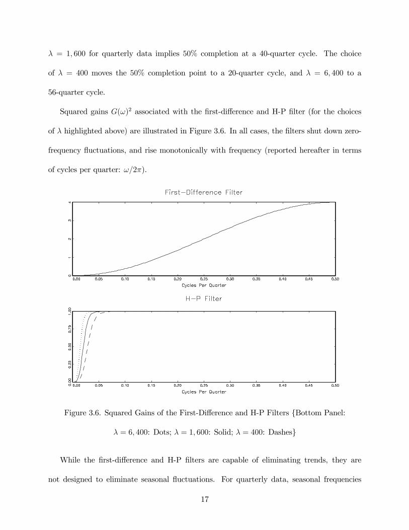
� = 1; 600 for quarterly data implies 50% completion at a 40-quarter cycle. The choice

of � = 400 moves the 50% completion point to a 20-quarter cycle, and � = 6; 400 to a

56-quarter cycle.

Squared gains G(!)2 associated with the �rst-di¤erence and H-P �lter (for the choices

of � highlighted above) are illustrated in Figure 3.6. In all cases, the �lters shut down zero-

frequency �uctuations, and rise monotonically with frequency (reported hereafter in terms

of cycles per quarter: !=2�).

Figure 3.6. Squared Gains of the First-Di¤erence and H-P Filters {Bottom Panel:

� = 6; 400: Dots; � = 1; 600: Solid; � = 400: Dashes}

While the �rst-di¤erence and H-P �lters are capable of eliminating trends, they are

not designed to eliminate seasonal �uctuations. For quarterly data, seasonal frequencies

17

correspond with 1=4 and 1=2 cycles per quarter, and the squared gains associated with each

of these �lters are positive at these values. As noted, business cycle models are not typically

designed to explain seasonal variation, thus it is desirable to work with variables that have

had seasonal variations eliminated.

As with the example analyzed above, it is most often the case that aggregate variables are

reported in seasonally adjusted (SA) form. Seasonal adjustment is typically achieved using

the so-called X-11 �lter (as characterized, e.g., by Bell and Monsell, 1992). So typically,

seasonal adjustment is not an issue of concern in the preliminary stages of an empirical

analysis. However, it is useful to consider this issue in order to appreciate the importance

of the seasonal adjustment step; the issue also serves to motive the introduction of the band

pass �lter, which provides an important alternative to the H-P �lter.

As an illustration of the importance of seasonal adjustment, Figure 3.7 presents the con-

sumption series discussed above, along with its non-seasonally-adjusted (NSA) counterpart

(including H-P trends for both). Trend behavior dominates both series, but the recurrent

seasonal spikes associated with the NSA series are distinctly apparent. The spikes are even

more apparent in Figure 3.8, which presents the H-P �ltered series.

18

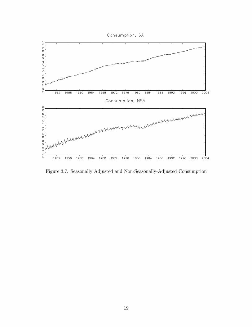
Figure 3.7. Seasonally Adjusted and Non-Seasonally-Adjusted Consumption

19

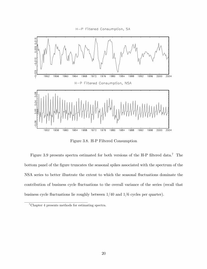
Figure 3.8. H-P Filtered Consumption

Figure 3.9 presents spectra estimated for both versions of the H-P �ltered data.7 The

bottom panel of the �gure truncates the seasonal spikes associated with the spectrum of the

NSA series to better illustrate the extent to which the seasonal �uctuations dominate the

contribution of business cycle �uctuations to the overall variance of the series (recall that

business cycle �uctuations lie roughly between 1=40 and 1=6 cycles per quarter).

7Chapter 4 presents methods for estimating spectra.

20

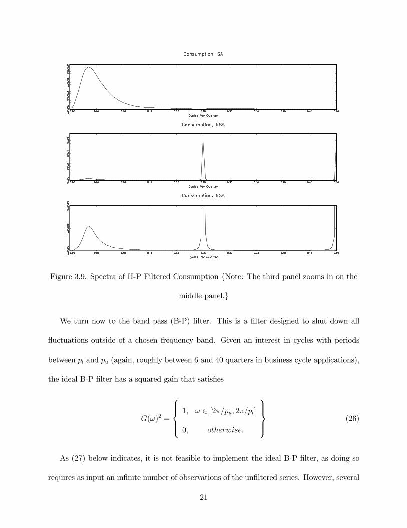
Figure 3.9. Spectra of H-P Filtered Consumption {Note: The third panel zooms in on the

middle panel.}

We turn now to the band pass (B-P) �lter. This is a �lter designed to shut down all

�uctuations outside of a chosen frequency band. Given an interest in cycles with periods

between pl and pu (again, roughly between 6 and 40 quarters in business cycle applications),

the ideal B-P �lter has a squared gain that satis�es

G(!)2 =

8>><>>:1; ! 2 [2�=pu; 2�=pl]

0; otherwise:

9>>=>>; (26)

As (27) below indicates, it is not feasible to implement the ideal B-P �lter, as doing so

requires as input an in�nite number of observations of the un�ltered series. However, several

21

approaches to estimating approximate B-P �lters have been proposed. Here, we present the

approach developed by Baxter and King (1999); for alternatives, e.g., see Woitek (1998) and

Christiano and Fitzgerald (1999).8

Let the ideal symmetric B-P �lter for a chosen frequency range be given by

�(L) =1X

j=�1�jL

j; (27)

where symmetry implies ��j = �j 8 j. This is an important property for �lters because it

avoids inducing what is known as a phase e¤ect. Under a phase e¤ect, the timing of events

between the un�ltered and �ltered series, such as the timing of business cycle turning points,

will be altered. The Fourier transformation of a symmetric �lter has a very simple form. In

the present case,

��e�i!

�� � (!) =

1Xj=�1

�je�i!j

= �0 +1Xj=1

�j�e�i!j + ei!j

�(28)

= �0 + 21Xj=1

�j cos(!);

where the second equality follows from symmetry and the last equality results from (22).

Baxter and King�s approximation to � (!) is given by the symmetric, �nite-ordered �lter

A(!) = a0 + 2

KXj=1

aj cos(!); (29)

8The collection of GAUSS procedures contained in bp.src are available for constructing Baxter andKing�s B-P �lter.

22

where A(0) =KP

j=�Kaj = 0, insuring that A(!) is capable of removing a trend from the

un�ltered series (see their Appendix A for details). A(!) is chosen to solve

minaj

�Z��

j� (!)� A (!) j2d! subject to A(0) = 0; (30)

i.e., A (!) minimizes departures from � (!) (measured in squared-error sense) accumulated

over frequencies. The solution to this objective is given by

aj = �j + �; j = �K; :::;K;

�j =

8>><>>:!u�!l�; j = 0

sin(!2j)�sin(!1j)�j

j = �1; :::; K;

9>>=>>; (31)

� =

�KP

j=�K�j

2K + 1;

where !l = 2�=pu and !u = 2�=pl.

Baxter and King propose the selection ofK = 12 in working with quarterly data, entailing

the loss of 12 �ltered observations at the beginning and end of the sample period. Figure

3.10 illustrates the squared gains associated with the ideal and approximated B-P �lters

constructed over the 1=40 and 1=6 cycles per quarter range.

23

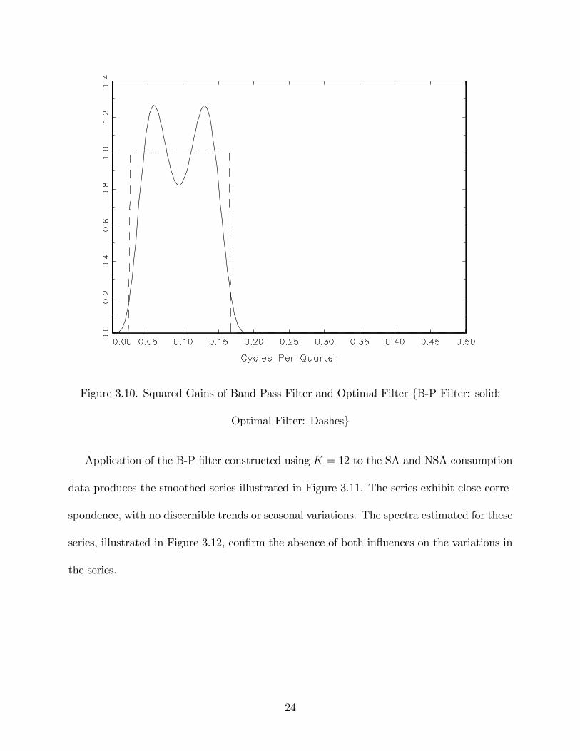
Figure 3.10. Squared Gains of Band Pass Filter and Optimal Filter {B-P Filter: solid;

Optimal Filter: Dashes}

Application of the B-P �lter constructed using K = 12 to the SA and NSA consumption

data produces the smoothed series illustrated in Figure 3.11. The series exhibit close corre-

spondence, with no discernible trends or seasonal variations. The spectra estimated for these

series, illustrated in Figure 3.12, con�rm the absence of both in�uences on the variations in

the series.

24

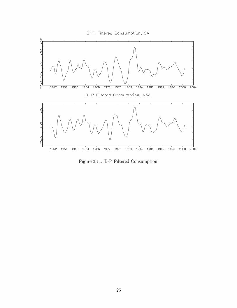
Figure 3.11. B-P Filtered Consumption.

25

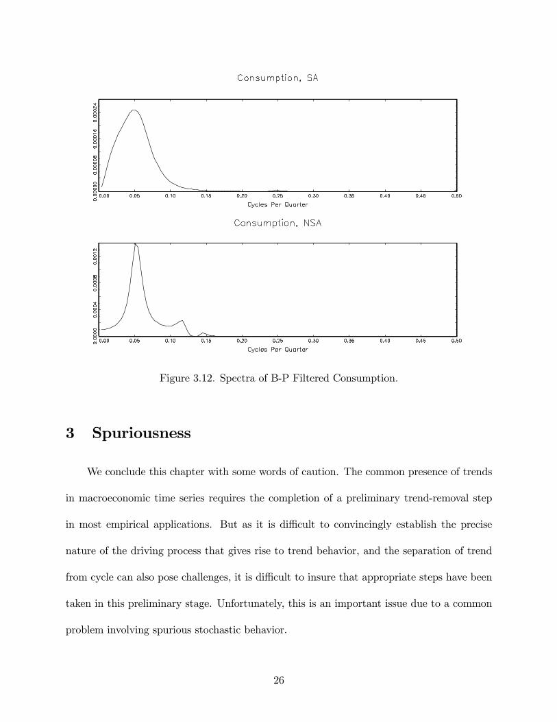
Figure 3.12. Spectra of B-P Filtered Consumption.

3 Spuriousness

We conclude this chapter with some words of caution. The common presence of trends

in macroeconomic time series requires the completion of a preliminary trend-removal step

in most empirical applications. But as it is di¢ cult to convincingly establish the precise

nature of the driving process that gives rise to trend behavior, and the separation of trend

from cycle can also pose challenges, it is di¢ cult to insure that appropriate steps have been

taken in this preliminary stage. Unfortunately, this is an important issue due to a common

problem involving spurious stochastic behavior.

26

In general, spuriousness is used to characterize situations in which the stochastic behavior

of a �ltered variable di¤ers systematically from its un�ltered counterpart along the dimension

of original interest in the empirical analysis. Of course, the stochastic behavior of the two

series will di¤er in general, but e.g., if the removal of a trend induces systematic di¤erences in

the business cycle properties of �ltered variables, spuriousness is said to have been induced.

Spuriousness can arise both in removing trends and isolating cycles. Regarding the

latter, consider the extreme but illustrative case in which an H-P or B-P �lter is applied to

a collection of zero-mean serially uncorrelated CSSPs. Such CSSPs are referred to as white

noise: their spectra are uniform. In this case, spectra of the �ltered series will identically

assume the shape of the squared gains of the �lters, and thus the �ltered series will exhibit

spurious cyclical behavior. Harvey and Jaeger (1993) provide an analysis of spurious behavior

arising from H-P �ltered data.

Regarding trend removal, we have seen that the removal of �xed trends from the levels of

series that have evidently undergone trend breaks can induce considerable persistence in the

detrended series. So even if the underlying data were trend-stationary, the application of a

�xed trend speci�cation in this case would induce undue persistence in the detrended series.

Moreover, as noted, it is di¢ cult to distinguish between trend- and di¤erence-stationary

speci�cations even given the ideal case of constant average growth over the sample period.

And as shown by Chan, Hayya and Ord (1977) and Nelson and Kang (1981), both the removal

of a deterministic trend from a di¤erence-stationary speci�cation and the application of the

di¤erence operator (1 � L) to a trend-stationary process induces spurious autocorrelation

in the resulting series. Similarly, Cogley and Nason (1995) and Murray (2003) illustrate

spuriousness arising from the application of the H-P and B-P �lters to non-stationary data.

27

Having painted this bleak picture, we conclude by noting that steps are available for

helping to mitigate these problems. For example, regarding the trend- versus di¤erence-

stationarity issue, while it is typically di¢ cult to reject either speci�cation in applications of

classical hypothesis tests to macroeconomic time series, it is possible to obtain conditional

inferences regarding their relative plausibility using Bayesian methods. Such inferences can

be informative in many instances.9 And the use of alternative �ltering methods in a given

application is a useful way to investigate the robustness of inferences to steps taken in this

preliminary stage.

9See DeJong and Whiteman (1991a,b) for examples in macroeconomic applications, and Phillips (1991)for skepticism. Tools for implementing Bayesian methods in general are presented in Chapter 9.

28

References

[1] Baxter, M. and R. G. King. 1999. �Measuring Business Cycles: Approximate Band-Pass

Filters for Economic Time Series.�Review of Economics and Statistics 81:575-593.

[2] Bell, W. R. and B. C. Monsell. 1992. �X-11 Symmetric Linear Filters and their Transfer

Functions.�Bureau of the Census Statistical Research Division Report Series No. RR-

92/15.

[3] Chan, K. J. C. Hayya, and K. Ord. 1977. �A Note on Trend Removal Methods: The

Case of Polynomial Versus Variate Di¤erencing.�Econometrica 45:737-744.

[4] Christiano, L. J. and T. J. Fitzgerald. 1999. �The Band Pass Filter.�Federal Reserve

Bank of Cleveland working paper.

[5] Cogley, T. and J. M. Nason. 1995. �E¤ects of the Hodrick-Prescott Filter on Trend and

Di¤erence Stationary Time Series: Implications for Business Cycle Research.�Journal

of Economic Dynamics and Control 19:253-278.

[6] DeJong, D. N. and C. H. Whiteman. 1991a. �The Temporal Stability of Dividends and

Prices: Evidence from the Likelihood Function.�Americal Economic Review 81:600-617.

[7] DeJong, D. N. and C. H. Whiteman. 1991b. �Trends and Random Walks in Macroeco-

nomic Time Series: A Reconsideration Based on the Likelihood Principle.�Journal of

Monetary Economics 28:221-254.

29

[8] DeJong, D. N. and C. H. Whiteman. 2003. �Unit Roots in U.S. Macroeconomic Time

Series: A Survey of Classical and Bayesian Methods.�In D. Brillinger et al., Eds. New

Directions in Time Series Analysis, Part II. Berlin: Springer-Verlag.

[9] Hamilton, J. D. 1994. Time Series Analysis. Princeton: Princeton University Press.

[10] Harvey, A. C. 1993. Time Series Models. Cambridge: MIT Press.

[11] Harvey, A. C. and A. Jaeger. 1993. �Detrending, Stylized Facts and the Business Cycle.�

Journal of Econometrics 8:231-247.

[12] Kaiser, R. and A. Maravall. 2001.Measuring Business Cycles in Economic Time Series.

Berlin: Springer-Verlag.

[13] Murray, C. J. 2003. �Cyclical Properties of Baxter-King Filtered Time Series.�Review

of Economics and Statistics 85:472-476.

[14] Nelson, C. and H. Kang. 1981. �Spurious Periodicity in Inappropriately Detrended Time

Series.�Econometrica 49:741-751.

[15] Nelson, C. and C. I. Plosser. 1982. �Trends and RandomWalks in Macroeconomic Time

Series.�Journal of Monetary Economics 10:139-162.

[16] Nordhaus, W. 2004. �Retrospective on the 1970s Productivity Slowdown.�NBERWork-

ing Paper 10950. Cambridge: NBER.

[17] Perron, P. 1989. �The Great Crash, the Oil Shock, and the Unit Root Hypothesis.�

Econometrica 57:1361-1401.

30

[18] Phillips, P. C. B. 1991. �To Criticize the Critics: An Objective Bayesian Analysis of

Stochastic Trends.�Journal of Applied Econometrics 6:333-364.

[19] Stock, J. H. 2004. �Unit Roots, Structural Breaks, and Trends.�In R. F. Engle and D.

L. McFadden, Eds. Handbook of Econometrics, Vol. 4. Amsterdam: North Holland.

[20] Wen, Y. 2002. �The Business Cycle E¤ects of Christmas.�Journal of Monetary Eco-

nomics 49:1289-1314.

[21] Woitek, Ulrich. 1998. �A Note on the Baxter-King Filter.�University of Glasgow work-

ing paper.

31