Structural vs. Atheoretic Approaches to Econometrics

Michael P. Keane1

ARC Federation Fellow University of Technology Sydney

and Research Fellow

Arizona State University

Abstract

In this paper I attempt to lay out the sources of conflict between the so-called “structural” and

“experimentalist” camps in econometrics. Critics of the structural approach often assert that it

produces results that rely on too many assumptions to be credible, and that the experimentalist

approach provides an alternative that relies on fewer assumptions. Here, I argue that this is a

false dichotomy. All econometric work relies heavily on a priori assumptions. The main

difference between structural and experimental (or “atheoretic”) approaches is not in the number

of assumptions but the extent to which they are made explicit.

JEL Codes: B23, C10, C21, C52, J24 Key Words: Structural Models, Natural Experiments, Dynamic Models, Life-cycle Models, Instrumental Variables

1 Address for correspondence: University of Technology Sydney, PO Box 123 Broadway NSW 2007 Australia, Phone: 61-2-9514-9742, Fax: 61-2-9514-9743, email: michael.keane@uts.edu.au.

1. Introduction

The goal of this conference is to draw attention to the many researchers, especially young

researchers, doing high quality structural econometric work in several areas of applied micro-

economics. It is motivated by a perception that structural work has fallen out of favor in recent

years, and that, as a result, the work being done by such young researchers has received too little

attention. Here, I’d like to talk about why structural work has fallen out of favor, whether that

ought to be the case, and, if not, what can be done about it. I’ll argue there is much room for

optimism, as recent structural work has increased our understanding of many key issues.

Since roughly the early 90s, a so-called “experimentalist” approach to econometrics has

been in vogue. This approach is well described by Angrist and Krueger (1999), who write that

“Research in a structuralist style relies heavily on economic theory to guide empirical work …

An alternative to structural modeling, … the “experimentalist” approach, … puts front and center

the problem of identifying causal effects from specific events or situations.” By “events or

situations,” they are referring to “natural experiments” that generate exogenous variation in

certain variables that would otherwise be endogenous in the behavioral relationship of interest.

The basic idea here is this. Suppose we are interested in the effect of a variable X on an

outcome Y, for example, the effect of an additional year of education on earnings. The view of

the “experimentalist” school is that this question is very difficult to address precisely because

education is not randomly assigned. People with different education levels tend to have different

levels of other variables U, at least some of which are unobserved (e.g., innate ability), that also

affect earnings. Thus, the “causal effect” of an additional year of education is hard to isolate.

However, the experimentalist school seems to offer us a way out of this difficult problem.

If we can find an “instrumental variable” Z that is correlated with X but uncorrelated with the

unobservables that also affect earnings, then we can use an instrumental variable (IV) procedure

to estimate the effect of X on Y. The “ideal instrument” is a “natural experiment” that generates

random assignment (or something that resembles it), whereby those with Z=1 tend, ceteris

paribus, to chose a higher level of X than those with Z=0. That is, some naturally occurring

event affects a random subset of the population, inducing at least some members of that

“treatment group” to choose or be assigned a higher level of X than they would have otherwise.2

2 As Angrist and Krueger (1999) state: “In labor economics at least, the current popularity of quasi-experiments stems … from this concern: Because it is typically impossible to adequately control for all relevant variables, it is often desirable to seek situations where it is reasonable to presume that the omitted variables are uncorrelated with

1

Prima facie, this approach doesn’t seem to require strong assumptions about how economic

agents chose X, or how U is generated.

This seemingly simple idea has found widespread appeal in the economics profession. It

has led to the currently prevalent view that, if we can just find “natural experiments” or “clever

instruments,” we can learn interesting things about behavior without making strong a priori

assumptions, and without using “too much” economic theory. In fact, I have heard it said that:

“empirical work is all about finding good instruments,” and that, conversely, results of structural

econometric analysis cannot be trusted because they hinge on “too many assumptions.” These

notions seem to account for both the current popularity of atheoretic approaches to econometrics,

and the relative disfavor into which structural work has fallen.

Here, I want to challenge the popular view that “natural experiments” offer a simple,

robust and relatively “assumption free” way to learn interesting things about economic

relationships. Indeed, I will argue that it is not possible to learn anything of interest from data

without theoretical assumptions, even when one has available an “ideal instrument.”3 Data

cannot determine interesting economic relationships without a priori identifying assumptions,

regardless of what sort of idealized experiments, “natural experiments” or “quasi-experiments”

are present in that data.4 Economic models are always needed to provide a window through

which we interpret data, and our interpretation will always be subjective, in the sense that it is

contingent on our model.

Furthermore, atheoretical “experimentalist” approaches do not rely on fewer or weaker

the variables of interest. Such situations may arise if … the forces of nature or human institutions provide something close to random assignment.” 3 By “data” I mean the joint distribution of observed variables. To use the language of the Cowles Commission, “Suppose … B is faced with the problem of identifying … the structural equations that alone reflect specified laws of economic behavior ... Statistical observation will in favorable circumstances permit him to estimate … the probability distribution of the variables. Under no circumstances whatever will passive statistical observation permit him to distinguish between different mathematically equivalent ways of writing down that distribution … The only way in which he can hope to identify and measure individual structural equations … is with the help of a priori specifications of the form of each structural equation” - see Koopmans, Rubin and Leipnik (1950). 4 The term “quasi-experiment” was developed in the classic work by Campbell and Stanley (1963). In the quasi-experiment, unlike a true experiment, subjects are not randomly assigned to treatment and control groups by the investigator. Rather, events that occur naturally in the field, such as administrative/legislative fiat, assign subjects to treatment and control groups. The ideal is that these groups appear very similar prior to the intervention, so that the event in the field closely resembles randomization. To gauge pre-treatment similarity, it is obviously necessary that the data contain a pre-treatment measure for the outcome of interest. Campbell and Stanley (1963) list several other types of research designs based on observational data which do not satisfy this criteria, such as studies based on “one-shot” cross-section surveys, which do not provide a pre-treatment outcome measure. They also emphasize that, even when treatment and control groups are very similar on observables prior to treatment, they may differ greatly on unobservables, making causal inferences from a quasi-experiment less clear than those from a true experiment.

2

assumptions than do structural approaches. The real distinction is that, in a structural approach,

ones a priori assumptions about behavior must be laid out explicitly, while in an experimentalist

approach key assumptions are left implicit. I will provide some examples of the strong implicit

assumptions that underlie certain “simple” estimators to illustrate this point.

Of course, this point is not new. For instance, Heckman (1997) and Rosenzweig and

Wolpin (2000) provide excellent discussions of the strong implicit assumptions that underlie

conclusions from experimentalist studies, accompanied by many useful examples. Nevertheless,

the perception that experimental approaches allow us to draw inferences without “too much”

theory seems to stubbornly persist. Thus, it seems worthwhile to continue to stress the fallacy of

this view. One thing I will try to do differently from the earlier critiques is to present even

simpler examples. Some of these examples are new, and I hope they will be persuasive to a

target audience that does not yet have much formal training in either structural or experimentalist

econometric approaches (i.e., first year graduate students).

If one accepts that inferences drawn from experimentalist work are just as contingent on

a priori assumptions as those from structural work, the key presumed advantage of the

experimentalist approach disappears. One is forced to accept that all empirical work in

economics, whether “experimentalist” or “structural,” relies critically on a priori theoretical

assumptions. But once we accept the key role of a priori assumptions, and the inevitability of

subjectivity, in all inference, how can we make more progress in applied work in general?

I will argue that this key role of a priori theory in empirical work is not really a problem

– its something economics has in common with other sciences – and that, once we recognize the

contingency of all inference, it becomes apparent that structural, experimentalist and descriptive

empirical work all have complimentary roles to play in advancing economics as a science.

Finally, I’ll turn to a critique of prior work in the structural genre itself. I will argue that

structural econometricians need to devote much more effort to validating structural models, a

point previously stressed in Wolpin (1996) and Keane and Wolpin (1997, 2007). This is a

difficult area, but I’ll describe how I think progress can be made.

2. Even “Ideal” Instruments Tell us Nothing Without A Priori Assumptions

When I argue we cannot ever learn anything from natural experiments without a priori

theoretical assumptions, a response I often get, even from structural econometricians, is this:

3

“you have to concede that when you have an ideal instrument, like a lottery number, results

based on it are incontrovertible.” In fact, this is a serious misconception that needs to be refuted.

One of the key papers that marked the rising popularity of the experimentalist approach was

Angrist (1990), who used Vietnam era draft lottery numbers – which were randomly assigned

but influenced the probability of “treatment” (i.e., military service) – as an instrument to estimate

the effect of military service on subsequent earnings. This paper provides an excellent illustration

of just how little can be learned without theory, even when we have such an “ideal” instrument.

A simple description of that paper is as follows: The sample consisted of men born from

‘50-‘53. The 1970 lottery affected men born in ‘50, the ’71 lottery affecting men born in ’51, etc.

Each man was assigned a lottery number from 1 to 365 based on random drawings of birth dates,

and only those with numbers below a certain ceiling (e.g., 95 in 1972) were draft eligible.

Various tests and physical exams were then used to determine the subset of draft eligible men

who were actually drafted into the military (which turned out to be about 15%). Thus, for each

cohort, Angrist runs a regression of earnings in some subsequent year (’81 through ’84) on a

constant and a dummy variable for veteran status. The instruments are a constant and a dummy

variable for draft eligibility. Since there are two groups, this leads to the Wald (1940) estimator,

)/()(ˆ NENE PPyy −−=β , where Ey denotes average earnings among the draft eligible group,

PP

E denotes the probability of military service for members of the eligible group, and Ny and PNP

are the corresponding values for the non-eligible group. The estimates imply that military service

reduced annual earnings for whites by about $1500 to $3000 in 1978$ (with no effect for blacks),

about a 15% decrease. The conclusion is that military service actually lowered earnings (i.e.,

veterans did not simply have lower earnings because they tended to have lower values of the

error term U to begin with).

While this finding seems interesting, we have to ask just what it means. As several

authors have pointed out, the quantitative magnitude of the estimate cannot be interpreted

without further structure. For instance, as Imbens and Angrist (1994) note, if effects of

“treatment” (e.g., military service) are heterogeneous in the population, then, at best, IV only

identifies the effect on the sub-population whose behavior is influenced by the instrument.5

5 As Bjorklund and Moffitt (1987) show, by using more structure, the average effect in the population, the average effect on those who are treated, and the effect on the marginal treated person, can all be uncovered in such a case. Heckman and Robb (1985) contains an early discussion of heterogeneous treatment effects. As Heckman and Vytlacil (2005) emphasize, when treatment effects are heterogeneous, the Imbens-Angrist interpretation that IV

4

As Heckman (1997) also points out, when effects of service are heterogeneous in the

population, the lottery number may not be a valid instrument, despite the fact that it is randomly

assigned. To see this, note that people with high lottery numbers (who will not be drafted) may

still choose to join the military if they expect a positive return from military service.6 But, in the

draft eligible group, some people with negative returns to military service are also forced to join.

Thus, while forced military service lowers average subsequent earnings among the draft eligible

group, the option of military service actually increases average subsequent earnings among the

non-eligible group. This causes the Wald estimator to exaggerate the negative effect of military

experience, either on a randomly chosen person from the population, or on the typical person

who is drafted, essentially because it relies on the assumption that y always falls with P.

A simple numerical example illustrates that the problems created by heterogeneity are not

merely academic. Suppose there are two types of people, both of whom would have subsequent

earnings of $100 if they do not serve in the military. Type 1’s will have a 20% gain if they serve,

and Type 2’s will have a 20% loss. Say Type 1’s are 20% of the population, and Type 2’s 80%.

So the average earnings loss for those who are drafted into service is –12%. Now, let’s say that

20% of the draft eligible group is actually drafted (while the Type 1’s volunteer regardless).

Then, the Wald estimator gives )(ˆ NE yy −=β /(PP

E –PNP ) = (100.8-104.0)/(.36-.20)= –20%. Notice

that this is the effect for the Type 2’s alone, who only serve if forced to by the draft. The Type

1’s don’t even matter in the calculation, because they increase both Ey and Ny by equal amounts.

If volunteering were not possible, the Wald estimator would instead give (97.6-100)/(.20-0) = –

12%, correctly picking out the average effect. The particular numbers chosen here do not seem

unreasonable (i.e., the percentage of draftees and volunteers is similar to that in Angrist’s SIPP

data on the 1950 birth cohort), yet the Wald estimator grossly exaggerates the average effect of

the draft.

Abstracting from these issues, an even more basic point is this: It is not clear from

Angrist’s estimates what causes the adverse effect of military experience on earnings. Is the estimates the effect of treatment on a subset of the population relies crucially on their monotonicity assumption. Basically, this says that when Z shifts from 0 to 1, a subset of the population is shifted into treatment, but no one shifts out. This is highly plausible in the case of draft eligibility, but is not plausible in many other contexts. In a context where the shift in the instrument may move people in or out of treatment, the IV estimator is rendered completely uninterruptible. I’ll give a specific example of this below. 6 Let Si be an indicator for military service, α denote the population average effect of military service, (αi-α) denote the person i specific component of the effect, and Zi denote the lottery number. We have that Cov(Si (αi -α), Zi)>0, since, among those with high lottery numbers, only those with large αi will choose to enlist.

5

return to military experience lower than that to civilian experience, or does the draft interrupt

schooling, or were there negative psychic or physical effects for the subset of draftees who

served in Vietnam (e.g., mental illness or disability), or some combination of all three? If the

work is to guide future policy, it is important to understand what mechanism was at work.

Rosenzweig and Wolpin (2000) stress that Angrist’s results tell us nothing about the

mechanism whereby military service affects earnings. For instance, suppose wages depend on

education, private sector work experience, and military work experience, as in a Mincer earnings

function augmented to include military experience. Rosenzweig and Wolpin note that Angrist’s

approach can only tell us the effect of military experience on earnings if we assume: (i)

completed schooling is uncorrelated with draft lottery number (which seems implausible as the

draft interrupts schooling) and (ii) private sector experience is determined mechanically as age

minus years of military service minus years of school. Otherwise, the draft lottery instrument is

not valid, because it is correlated with schooling and experience, which are relegated to the error

term – randomization alone does not guarantee exogeneity.

Furthermore, even these conditions are necessary but not sufficient. It is plausible that

schooling could be positively or negatively affected by a low lottery number, as those with low

numbers might (a) stay in school to avoid the draft, (b) have their school interrupted by being

drafted, or (c) receive tuition benefits after being drafted and leaving the service. These three

effects might leave average schooling among the draft eligible unaffected - so that (i) is satisfied

- yet change the composition of who attends school within the group.7 With heterogeneous

returns to schooling, this compositional change may reduce average earnings of the draft eligible

group, causing the IV procedure to understate the return to military experience itself.8

7 E.g., some low innate ability types get more schooling in an effort to avoid the draft, some high innate ability types get less schooling because of the adverse consequence of being drafted and having school interrupted. 8 As an aside, this scenario also provides a good example of the crucial role of monotonicity stressed by Heckman and Vytlacil (2005). Suppose we use draft eligibility as an IV for completed schooling in an earnings equation, which – as noted somewhat tongue-in-cheek by Rosenzweig and Wolpin (2000) – seems prima facie every bit as sensible as using it as an IV for military service (since draft eligibility presumably affects schooling while being uncorrelated with U). Amongst the draft eligible group, some stay in school longer than they otherwise would have, as a draft avoidance strategy. Others get less schooling than they otherwise would have, either because their school attendance is directly interrupted by the draft, or because the threat of school interruption lowers the option value of continuing school. Monotonicity is violated since the instrument, draft eligibility, lowers school for some and raises it for others. Here, IV does not identify the effect of schooling on earnings for any particular population subgroup. Indeed, the IV estimator is completely un-interpretable. In the extreme case described in the text, where mean schooling is unchanged in the draft eligible group (i.e., the flows in and out of school induced by the instrument cancel), and mean earnings in the draft eligible group are reduced by the shift in composition of who attends school, the plim of the Wald estimator is undefined, and its value in any finite sample is completely meaningless.

6

Another important point is that the draft lottery may itself affect behavior. That is,

people who draw low numbers may realize that there is a high probability that their educational

or labor market careers will be interrupted. This increased probability of future interruption

reduces the return to human capital investment today.9 Thus, even if they are not actually

drafted, men who draw low lottery numbers may experience lower subsequent earnings because,

for a time, their higher level of uncertainty caused them to reduce their rate of investment. This

would tend to lower Ey relative to Ny , exaggerating the negative effect of military service per

se.10

This argument may appear to be equivalent to saying that the lottery number belongs in

the main outcome equation, which is to some extent a testable hypothesis. Indeed, Angrist (1990)

performs such a test. To do this, he disaggregates the lottery numbers into 73 groups of 5, that is,

1-5, 6-10, …, 361-365. This creates an over-identified model, so one can test if a subset of the

instruments belongs in the main equation. To give the intuitive idea, suppose we group the

lottery numbers into low, medium and high, and index these groups by j=1, 2, 3. Then, defining

PP

j = P(S =1|Z∈j), the predicted military service probability from a first stage regression of

service indicators on lottery group dummies, we could run the second stage regression: i i

(1) ij

ii PZIy εαββ ++∈+= ]1[10

where yi denotes earnings of person i at some subsequent date. Given that there are three groups

of lottery numbers, we can test the hypothesis that the lottery numbers only matter through their

effect on the military enrolment probability PP

j by testing if β , the coefficient on an indicator for

a low lottery number, is significant. Angrist (1999) conducts an analogous over-identification

test (using all 73 instrument groups, and also pooling data from multiple years and cohorts), and

does not reject the over-identifying restrictions.

1

11

However, this test does not actually address my concern about how the lottery may affect

behavior. In my argument, a person’s lottery number affects his rate of human capital investment

9 Note that draft number cutoffs for determining eligibility were announced some time after the lottery itself, leaving men uncertain about their eligibility status in the interim. 10 Heckman (1997), footnote 8, contains some similar arguments, such as that employers will invest more (less) in workers with high (low) lottery numbers. 11 Unfortunately, many applied researchers are under the false impression that over-identification tests allow one to test the assumed exogeneity of instruments. In fact, such tests require that at least one instrument be valid (which is why they are over-identification tests), and this assumption is not testable. To see this, note that we cannot also include I[Zi ∈ 2] in (1), as this creates perfect collinearity. As noted by Koopmans, Rubin and Marsckak (1950), “… the distinction between exogenous and endogenous variables is a theoretical, a prior distinction …”

7

through its affect on his probability of military service. Thus, I am talking about an effect of the

lottery that operates through PP

j, but that is (i) distinct from the effect of military service itself,

and (ii) would exist within the treatment group even if none were ultimately drafted. Such an

effect cannot be detected by estimating (1), because the coefficient α already picks it up.

To summarize, it is impossible to meaningfully interpret Angrist’s –15% estimate without

a priori theoretical assumptions. Under one (strong) set of assumptions, the estimate can be

interpreted to mean that, for the subset of the population induced to serve by the draft (i.e., those

who would not have otherwise voluntary chosen the military), mean earnings were 15% lower in

the early 80s than they would have been otherwise. But this set of assumptions rules out various

plausible behavioral responses by the draft eligible who were not ultimately drafted.

3. Interpretation is Prior to Identification

Advocates of the “experimentalist” approach often criticize structural estimation because,

they argue, it is not clear how parameters are “identified.” What is meant by “identified” here is

subtly different from the traditional use of the term in econometric theory – i.e., that a model

satisfies technical conditions insuring a unique global maximum for the statistical objective

function. Here, the phrase “how a parameter is identified” refers instead to a more intuitive

notion that can be roughly phrased as follows: What are the key features of the data, or the key

sources of (assumed) exogenous variation in the data, or the key a priori theoretical or statistical

assumptions imposed in the estimation, that drive the quantitative values of the parameter

estimates, and strongly influence the substantive conclusions drawn from the estimation

exercise?

For example, Angrist (1995) argues: “’Structural papers’ … often list key identifying

assumptions (e.g., the instruments) in footnotes, at the bottom of a table, or not at all. In some

cases, the estimation technique or write up is such that the reader cannot be sure just whose (or

which) outcomes are being compared to make the key causal inference of interest.”

In my view, there is much validity to Angrist’s criticism of structural work here. The

main positive contribution of the “experimentalist” school has been to enhance the attention that

empirical researchers pay to identification in the more intuitive sense noted above. This emphasis

has also encouraged the formal literatures on non-parametrics and semi-parametrics that ask

useful questions about what assumptions are essential for estimation of certain models, and what

8

assumptions can be relaxed or dispensed with.12

However, while it has brought the issue to the fore, the “experimentalist” approach to

empirical work per se has not helped clarify issues of identification. In fact, it has often tended to

obscure them. The Angrist (1990) draft lottery paper again provides a good illustration. It is

indeed obvious what the crucial identifying assumption is: A person’s draft lottery number is

uncorrelated with his characteristics, and only influences his subsequent labor market outcomes

through its affect on his probability of veteran status. Nevertheless, despite this clarity, it is not at

all clear or intuitive what the resultant estimate of the effect of military service on earnings of

about –15% really means, or what “drives” that estimate.

As the discussion in the previous section stressed, many interpretations are possible. Is it

the average effect, meaning the expected effect when a randomly chosen person from the

population is drafted? Or, is the average effect much smaller? Are we just picking out a large

negative effect that exists for a subset of the population? Is the effect a consequence of military

service itself, or of interrupted schooling or lost experience? Or do higher probabilities of being

drafted lead to reduced human capital investment due to increased risk of labor market

separation? I find I have very little intuition for what drives the estimate, despite the clarity of the

identifying assumption.

This brings me to two more general observations about atheoretical work that relies on

“natural experiments” to generate instruments:

First, exogeneity assumptions are always a priori, and there is no such thing as an “ideal”

instrument that is "obviously" exogeneous. We’ve seen that even a lottery number can be

exogeneous or endogeneous, depending on economic assumptions. “Experimentalist” approaches

don't clarify the a priori economic assumptions that justify an exogeneity assumption, because

work in that genre typically eschews being clear about the economic model that is being used to

interpret the data. When the economic assumptions that underlie the validity of instruments are

left implicit, the proper interpretation of inferences is obscured.

Second, interpretability is prior to identification. “Experimentalist” approaches are

typically very "simple" in the sense that if one asks, “How is a parameter identified?,” the answer

is "by the variation in variable Z , which is assumed exogenous." But, if one asks “What is the

meaning or interpretation of the parameter that is identified?” there is no clear answer. Rather, 12 See Heckman and Navarro (2007), or Heckman, Matzkin and Nesheim (2005) and the discussion in Keane (2003), for good examples of this research program.

9

the ultimate answer is just: "It is that parameter which is identified when I use variation in Z."

I want to stress that this statement about the lack of interpretability of atheoretic, natural

experiment based, IV estimates is not limited to the widely discussed case where the “treatment

effect” is heterogeneous in the population. As we know from Imbens and Angrist (1994), and as

discussed in Heckman (1997), when treatment effects are heterogeneous, as in the equation yi =

β0 + β1i Xi + ui, the IV estimator based on instrument Zi identifies, at best, the “effect” of X on

the subset of the population whose behavior is altered by the instrument. Thus, our estimate of

the “effect” of X depends on what instrument we use. All we can say is that IV identifies “that

parameter which is identified when I use variation in Z.” Furthermore, as noted by Heckman and

Vytlacil (2005), even this ambiguous interpretation hinges on the monotonicity assumption,

which requires that the instrument shift subjects in only one direction (either into or out of

treatment). But, as I will illustrate in Section 4, absent a theory, this lack of interpretability of IV

estimates even applies in homogenous coefficient models.

In a structural approach, in contrast, the parameters have clear economic interpretations.

In some cases, the source of variation in the data that identifies a parameter or drives the

behavior of a structural model may be difficult to understand, but I do not agree that such lack of

clarity is a necessary feature of structural work. In fact, in Section 5, I will give an example of a

structural estimation exercise where (i) an estimated parameter has a very clear theoretical

interpretation, and (ii) it is perfectly clear what patterns in the data “identify” the parameter in

the sense of driving its estimated value. In any case, it does not seem like progress to gain clarity

about the source of identification while losing interpretability of what is being identified!

4. The General Ambiguity of IV Estimates Absent a Theory

The problem that atheoretic IV type estimates are difficult to interpret is certainly not

special to Angrist’s draft lottery paper, or, contrary to a widespread misperception, special to

situations where “treatment effects” are heterogeneous. As another simple example, consider

Bernal and Keane (2007).13 This paper is part of a large literature that looks at effects of

maternal contact time – specifically, the reduction in contact time that occurs if mothers work

and place children in child care – on child cognitive development (as measured by test scores).

13 By discussing one of my own papers, I hope to emphasize that my intent is not to criticize specific papers by others, like the Angrist (1990) paper discussed in Section 2, but rather to point out limitations of the IV approach in general.

10

Obviously, we can’t simply compare child outcomes between children who were and were not in

day care to estimate the “effect” of day care, because it seems likely that mothers who work and

place children in day care are different from mothers who don’t. Thus, what researchers typically

do in this literature is regress a cognitive ability test score measured at, say, age 5, on a measure

of how much time a child spent in day care up through age five, along with a set of “control

variables,” like the mother’s education and AFQT score, meant to capture the differences in

mothers’ cognitive ability endowments, socio-economic status, and so on.

But even with the most extensive controls available in survey data, there are still likely to

be unobserved characteristics of mothers and children that are correlated with day care use. Thus,

we’d like to find a “good” instrument for day care – a variable or set of variables that influences

maternal work and day care choices, but is plausibly uncorrelated with mother and child

characteristics. Bernal and Keane (2007) argue the existing literature in this area hasn’t come up

with any good instruments, and propose that the major changes in welfare rules in the U.S. in the

90s are a good candidate. These rule changes led to substantial increases in work and day care

use among single mothers, as the aim of the reforms was to encourage work. And it seems very

plausible that the variation in welfare rules over time and across States had little or no correlation

with mother and child characteristics. So, as far as instruments go, I think this is about as good as

it gets.

Now, I think it is fair to say that, in much recent empirical work in economics, a loose

verbal discussion like that in the last two paragraphs is all the “theory” one would see. It would

not be unusual to follow the above discussion with a description of the data, run the proposed IV

regression, report the resultant coefficient on day care as the “causal effect” of day care on child

outcomes, and leave it at that. In fact, when we implement the IV procedure, we get -.0074 as the

coefficient on quarters of day care in a log test score equation (standard error .0029), implying

that a year of day care lowers the test score by 3.0%, which is .13 standard deviations of the

score distribution. But what does this estimate really mean? Absent a theoretical framework, it is

no more interpretable than Angrist’s –15% figure for the “effect” of military service on earnings.

One way to provide a theoretical framework for interpreting the estimate is to specify a

child cognitive ability production function. For concreteness, I’ll write this as:

iitititit GCTA ωαααα ++++= lnln 3210 (2)

where Ait is child i‘s cognitive ability t periods after birth (assumed to be measured with classical

11

error by a test score), itT , itC and itG are the cumulative maternal time, day-care/pre-school time,

and goods inputs up through age t,14 and ωi is the child’s ability endowment. The key issue in

estimating (2) is that itT , itG and ωi are not observed in available data sets. As a consequence,

the few studies that actually have a production framework in mind15 sometimes use household

income Iit (and perhaps prices of goods) as a “proxy” for Git. It is also typical to assume a

specific relationship between day care time and maternal time, so that itT drops out of the

equation, and to include mother characteristics like education to proxy for ωi. What are the

effects of these decisions?

In a related context, Rosenzweig and Schultz (1983) discussed the literature on birth

weight production functions. They noted that studies of effects of inputs like prenatal care on

birth weight had typically dealt with problems of missing inputs, such as maternal nutrition, by

including in the equation their determinants, such as household income and food prices. They

referred to such an equation, which includes a subset of inputs along with determinants of the

omitted inputs, as a “hybrid” production function, and noted that estimation of such an equation

does not in general recover the ceteris paribus effects of the inputs on the outcome of interest.

In the cognitive ability production case, the use of household income to proxy for goods,

and the assumption of a specific relationship between day care and maternal time, also leads to a

“hybrid” production function. To interpret estimates of such an equation – and in particular to

understand conditions under which they reveal the ceteris paribus effect of the day care time

input on child outcomes – we need assumptions on how inputs are chosen, as I now illustrate.

First, decompose the child’s ability endowment into a part that is correlated with a vector

of characteristics of the mother, Ei, such as her education, and a part iω̂ that is mean independent

of the mother’s characteristics, as follows:

iii E ωββω ˆ10 ++=

Second, assume (as in the Appendix) a model where mothers choose four endogenous

variables: hours of work, maternal “quality” contact time, day-care/pre-school time, and goods

14 The goods inputs would include things like books and toys that enhance cognitive development. The day-care/pre-school inputs would include contributions of alternative care providers’ time to child cognitive development. These may be more or less effective than mother’s own time. In addition, care in a group setting may contribute to the child’s development by stimulating interaction with other children, learning activities at pre-school, etc.. 15 Besides Bernal and Keane (2007), I am thinking largely of James-Burdumy (2005), Bernal (2007), Blau (1999) and Leibowitz (1977).

12

inputs. The exogenous factors that drive these choices are the mother’s wage (determined by her

education and productivity shocks), the child’s skill endowment, the welfare rules and price of

child care, and the mother’s tastes for leisure and child care use. In such a model, the mother’s

decision rule (demand function) for the child care time input at age t, Cit, can of course be written

as a function of the exogenous variables, which for simplicity I assume is linear:

cititiiit RccEC εππωπππ +++++= 43210 ˆ

Here cc is the price per unit of day care time that the mother faces at time t, Rit is a set of welfare

program rules facing the mother at time t, and is a stochastic term that subsumes several

factors, including tastes for child care use, shocks to child care availability, and shocks to the

mother’s offered wage rate. [The fact that the price of child-care cc is assumed constant over

mothers/time is not an accident. A key problem confronting the literature on child-care is that the

geographic variation in cc seems too modest to use it as an IV for child-care usage.]

citε

Third, we need expressions for the unobserved goods and maternal “quality” time inputs

as a function of observed endogenous and exogenous variables (and stochastic terms), so that we

can substitute the unobserved endogenous variables out of (2). In a model with multiple jointly

determined endogenous variables (y1, y2) we can generally adopt a two-stage solution (i.e., solve

for optimal y2 as a function of y1, and then optimize with respect to y1). For simplicity, I assume

the optimal levels of the cumulative inputs of maternal time, itT , and goods, itG , up through age

t can be written, conditional on the cumulative child care and hours inputs, as follows:

gititititiiit

Tititititiiit

tRHWIHCEG

RHWIHCtET

εγγγγωγγγ

εφφφωφφφ

+++++++=

++++⋅++=

6543210

543210

);,(lnˆln

);,(ln)ˆ( (3)

The Appendix illustrates how, in a simple static model, such relationships, which I will call

“conditional decision rules,” can be obtained as the second stage in an optimization process,

where, in the first stage, the mother chooses the child-care time inputs C and hours of market

work H. Typically, an analytic derivation is not feasible in a dynamic model, so the equations in

(3) can be viewed as simple linear approximations to the more complex relationships that would

exist given dynamics. The notation );,( RHWIit highlights the dependence of income on wages,

hours of market work, and the welfare rules R that determine how benefits depend on income.

I won’t spend a great deal of time defending the specifications in (3), as they are meant to

be illustrative, and as they play no role in estimation itself, but are used only to help interpret the

13

estimates. The key thing captured by (3) is that a mother’s decisions about time and goods inputs

into child development may be influenced by (i.e., made jointly with) her decisions about hours

of market work and child-care. Both equations capture the notion that per-period inputs depend

on the mother’s characteristics E (which determine her level of human capital), and the child’s

ability endowment iω̂ . The time trends in (3) capture the growth of cumulative inputs over time.

Now, if we substitute the equations for ωi, Tit and lnGit into (2), we obtain:

}ˆˆ)1{(

)(})({)(

ln)()()(ln

312123

131631014341

5351333120030

git

Titii

iiit

ititit

t

EtEH

ICA

εαεαωφαωγα

γαβγαφφαγαφα

γαφαγαφααβγαα

+++++

⋅++⋅+++++

++⋅+++++=

(4)

This “hybrid” production function is estimable, since the independent variables are typically

measurable in available data sets. But the issues of choice of an appropriate estimation method,

and proper interpretation of the estimates, are both subtle.

The first notable thing about (4) is that the composite error term contains the unobserved

part of the child’s ability endowment, iω̂ , as well as the stochastic terms and , which

capture mothers’ idiosyncratic tastes for investment in child quality via goods and time inputs. It

seems likely that child-care usage, cumulative income and cumulative labor market hours are

correlated with all of these error components. For the welfare rule parameters R

gitε

Titε

it to be valid

instruments for cumulative child care and income in estimating (4), they must be uncorrelated

with these three error components, which seems like a plausible exogeneity assumption.

Assuming that IV based on R provides consistent estimates of (4), it is important to

recognize that the child-care “effect” that is estimated is (α2 + α1φ3 + α3γ3). This is the “direct”

effect of child-care time (α2), holding other inputs fixed, plus indirect effects arising because the

mother’s quality time input (α1φ3) and the goods input (α3γ3) also vary as child-care time varies.

While α1, α2, and α3 are structural parameters of the production technology (2), the parameters φ3

and γ3 come from the conditional decision rules for time and goods inputs (3), which are not

necessarily policy invariant. This has implications for both estimation and interpretation.

First, a valid instrument for estimation of (4) must have the property that it does not alter

the parameters in (3). A good example of a prima facie plausible instrument that does not have

this property is the price of child-care. Variation in this price will shift the conditional decision

rule parameters, since it shifts the mother’s budget constraint conditional on C, H and I. In

14

contrast, a change in welfare rules that determine how benefits affect income does not have this

problem, since such a change is reflected in I(W, H; R).

Second, given consistent estimates of (4), the estimated “effect” of child-care usage on

child cognitive outcomes applies only to policy experiments that do not alter the conditional

decision rules for time and goods investment in children (3). As these decision rules are

conditional on work, income and child-care usage decisions, they should be invariant to policies

that leave the budget constraint conditional on those decisions unchanged. A work requirement

that induces a woman to work and use child-care, but that leaves her wage rate and the cost of

care unaffected, would fall into this category. But day care subsidies would not.

Third, absent further assumptions, estimates of (4) cannot tell us if maternal time is more

effective at producing child quality than child-care time. For instance, if φ3>-1 then mother’s

“quality” time with the child is reduced less than one-for-one as day-care time is increased.

Then, the estimated day care “effect” may be zero or positive even if α2 < α1 and α3γ3 = 0.16

In contrast, consider a model where maternal contact time with the child is just a

deterministic function of day care use, as in Tit = T-Cit, where T is total time in a period. That is,

we no longer make a distinction between total contact time and “quality” time.17 In that case, we

get φ0=T, φ1=φ2=φ4=φ5=0, φ3= -1, so that itit CtTT −⋅= , and we obtain the simpler expression

(α2 - α1) + α3γ3 for the coefficient on itC in (4). This is the effect of day care time relative to

maternal time, plus the impact of any change in the goods input that the mother implements to

compensate for the reduction in the maternal time input. To resolve the ambiguity regarding the

impact of maternal time relative to child-care time, we need to impose some prior on reasonable 16 To my knowledge, James-Burdumy (2005) is the first paper in the day care literature that notes the ambiguity in the estimated “effect” of day care that arises because, in general, the maternal quality time input may also be varied (via optimizing behavior of the mother) as child care time is varied. On a related point, Todd and Wolpin (2003), provide a good discussion of the proper interpretation of production function estimates when proxy variables are used to control for omitted inputs. For instance, say one includes in the production function a specific maternal time input, like time spent reading to the child, along with a proxy for the total maternal time input (say, maternal work and day care use, which reduce total maternal care time). Then, the coefficient on reading time captures the effect of reading time holding total time fixed, implying that time in some other activities must be reduced. Of course, excluding the proxy does not solve the problem, as the coefficient on reading time then captures variation of the omitted inputs with reading time. This is similar to the problem we note here, where the change in day care time may be associated with changes in other unmeasured inputs (i.e., maternal quality time or goods inputs). 17 In the Appendix, I consider a model where C-H is the mother’s private leisure time, while T-C is the total time the child is in the mothers care. The mother chooses how much of the latter to devote to “quality” time with the child vs. other types of non-market activity (e.g., the child’s time could be divided between day-care, “quality” time with the mother, and time spent watching TV while the mother does housework). It is only to the extent that C>H for some mothers that one can include both C and H in (3). In fact, Bernal and Keane (2007) find that C and H are so highly correlated for single mothers that they cannot both be included in (4).

15

magnitudes of α3γ3. Only in a model with γ3 = 0, so that goods inputs are invariant to the child-

care input,18 does IV identify the structural (or policy invariant) parameter (α2 - α1), the effect of

time in child-care relative to the effect of mother’s time.

Thus, what is identified when one regresses child outcomes on day care, using welfare

policy rules as an instrument, along with income as a proxy for goods inputs, and mother socio-

economic characteristics as “control” variables, may or may not be a structural parameter of the

production technology, depending on a priori economic assumptions.19 IV estimates of (4) are

not interpretable without specifying these assumptions.

Rosenzweig and Wolpin (1980a, b) pointed out the fundamental under-identification

problem that arises in attempts to distinguish child quality production function parameters from

mother’s (or parent’s) utility function parameters in household models. For instance, suppose we

observe a “natural experiment” that reduces the cost of child-care. Say this leads to a substantial

increase in child-care use and maternal work, and only a small drop in child test outcomes. We

might conclude child-care time is a close substitute for mother’s time in child quality production.

But we might just as well conclude that the cross-price effect of child-care cost on

demand for child quality is small (e.g., because the household is very unwilling to substitute

consumption or leisure for child quality). Then, the increase in child-care use is accompanied by

a substantial increase in the goods input into child quality production, and/or mother’s quality

time input may be reduced much less than one-for-one. Absent strong assumptions, we can’t

disentangle production function parameters from properties of the household’s utility function

using estimates of (4).20 As Rosenzweig and Wolpin (1980a, b) note, even the “ideal” natural

experiment that randomly assigns children to different levels of day-care does not resolve this

problem. One can only distinguish production from utility function parameters using a priori

theoretical assumptions. 18 If γ3 = 0, the log goods input is a linear function of log income and hours of market work, which appear in (4), but not of child care time. It is interesting that, in this case, where we have also set φ4=0, the maternal work hours coefficient in (4) does not capture an effect of maternal time at all, but rather an association between work hours and the goods input (α3 γ4). 19 Rosenzweig and Wolpin (2000) give other examples where the parameter that IV based on “truly random” instruments identifies depends on (i) the control variables that are included in the “main” equation, (ii) the maintained economic assumptions. Most notably, these examples include (i) estimates of the “causal effect” of education on earnings, using date of birth or gender of siblings as instruments, and (ii) estimates of effects of transitory income shocks on consumption, using weather as an instrument for farm income. 20 Obviously, direct measures of “quality” time and goods inputs would alleviate this problem. But, to make use of such data requires other assumptions. For instance, one would need to define “quality” time, and make assumptions about whether various types of quality time also enter the mother’s utility directly. Similarly, one would need to classify goods into those that enter quality production vs. ones that also enter utility directly vs. ones that do both.

16

5. Cases Where there Are No Possible Instruments

In this section I’ll examine the limitations of IV from another perspective, by looking at a

case where an important structural parameter of interest cannot be identified using IV, even

under “ideal” conditions. In that case, only a fully structural approach is possible.

Consider a “standard” life cycle labor supply model, with (i) agents free to borrow and

lend across periods at a fixed interest rate r, (ii) wages evolving stochastically but exogenously,

and (iii) period utility separable between consumption and leisure, and given by u(ct, lt) = v(ct) –

b(t) , α>1, where cαth t , lt and ht are consumption, leisure and hours of work, respectively, and

b(t) is a time varying shift to tastes for leisure. This generates the Frisch labor supply function:

[ )(lnlnlnln1

1ln tbWh ttt −−+−

= αλα

]

]

(5)

where Wt is the wage rate at age t, and λt is the marginal utility of wealth (see MaCurdy, 1981).

Note that η ≡ 1/(α-1) = ∂lnht/∂lnWt, the intertemporal elasticity of substitution, is a key

parameter of interest, as it determines both how agents respond to anticipated changes in wages

over the life-cycle (as anticipated changes do not affect the marginal utility of wealth), and how

agents respond to transitory wage shocks, regardless of whether they are anticipated or not (since

a transitory shock, even if unanticipated, has little effect on λt). Given its importance in both

labor economics and macroeconomics, a large literature is devoted to estimating this parameter.

Now, estimation of (5) is complicated by the fact that the marginal utility of wealth λt is

unobserved. However, its change can be approximated by ∆ln λt ≈ (ρ-r) + εt, where ρ is the

discount rate and εt is a shock to the marginal utility of wealth that arises because of new

information that is revealed between ages t-1 and t. Hence, a number of papers work with a

differenced version of (5), given by:

)(ln[)(lnln ttt tbrWh εηρηη +Δ+−+Δ=Δ (6)

Equation (6) cannot be estimated using OLS, because of the problem that ∆lnWt and εt are likely

to be correlated. That is, the change in wages from t-1 to t is likely to contain some surprise

component that shifts the marginal utility of wealth, generating an income effect. However,

under the assumptions of the model, a valid instrument for ∆lnWt is a variable Zt that has the

properties: (i) it predicts wage growth from t-1 to t, (ii) it was known at time t-1, and hence is

uncorrelated with εt, and (iii) it is uncorrelated with the change in tastes b(t) from t-1 to t.

Typically, the instruments that have been used to identify the structural parameter η are

17

variables like age, age2 and age·education. These variables predict wage growth between t-1 and

t, because of the well know “hump shape” in the life-cycle earnings profile – that is, earnings

tend to grow quickly age young ages, but they grow at a decreasing rate with age, until reaching

a peak in roughly the late 40s or early 50s, after which they begin to head down. Also, the shape

of the profile differs somewhat by education level, so age·education has predictive power as

well. On the other hand, age at t is known at t-1, as is education (provided the person had already

finished the school and entered the labor force), so these variables satisfy requirement (ii).21

Now, given our theoretical assumptions, the interpretation of η in (6) is quite clear.

Furthermore, the source of identification when we estimate (6) using variables like age, age2 and

age·education as instruments is also quite clear. What will drive the estimate of η is how hours

vary over the life-cycle as wages move along the predictable life-cycle age path. In other words,

we identify η from the low frequency co-variation between hours and wages over the life-cycle.

Table 1 presents statistics from the NLSY79 on growth in wages and hours for young

men. That data is described in detail in Imai and Keane (2004), so I won’t go into details here.

From age 24 to age 31, the average wage rate increases from $7.07 per hour to $9.66 per hour, a

36.6% increase. Meanwhile, average hours increase from 2034 to 2290, only a 12.6% increase. A

back-of-the-envelope calculation suggests an inter-temporal elasticity of substitution of roughly

12.6/36.6 = .34. Not surprisingly, when Imai and Keane (2004) use these data to estimate η using

the IV procedure described above, they get .26, with a standard error of .077 (see their Table 6).

Every researcher who has estimated the inter-temporal elasticity of substitution for men, using a

similar procedure, has obtained a similarly low estimate. It is very clear what pattern in the data

drives the estimate: wages rise much more over the life-cycle path than do hours, in percentage

terms. If we look at the data through the lens of the “standard” life-cycle model with exogenous

wages, this implies the inter-temporal elasticity of substitution must be small.

Imai and Keane (2004) show how one comes to a very different conclusion by viewing

the data through the lens of a model with endogenous wages. They consider a model where work

experience increases wages through a learning-by-doing mechanism. In that case, the wage rate

21 Whether age and education are also uncorrelated with changes in tastes for leisure is a problematic issue I’ll leave aside here. The typical paper in this literature uses variables like marital status and number of children to control for life-cycle factors that may systematically shift tastes for leisure. Another difficult issue is how to deal with aggregate shocks in estimation of (6). Most authors use time dummies to pick up both aggregate taste shocks and the annual interest rate terms. But Altug and Miller (1989) pointed out that time dummies only control for aggregate shocks if those shocks shift the marginal utility of consumption for all agents in the same way – which is tantamount to assuming complete markets.

18

Wt is no longer equal to the opportunity cost of time. Let tW~ denote the true opportunity cost of

time, which now equals the current wage plus the present discounted value of increased future

earnings that results from working an extra hour today. In that case, equation (6) becomes:

])(ln)ln~ln[()(lnln ttttt tbWWrWh εηρηη +Δ+Δ−Δ+−+Δ=Δ (7)

Note that the difference ln tW~ -lnWt between the opportunity cost of time and the wage rate now

enters the composite error term in square brackets. Due to the horizon effect, the return to human

capital investment declines with age. Thus, age is correlated with the error term, and is not a

valid instrument for estimating η. Similarly, if the level of human capital enters the human

capital production function (e.g., due to diminishing returns to human capital investment), then

any variable that affects the level of human capital, like education, is not a valid instrument

either.

In fact, I would argue that there are no valid instruments by construction. Any variable

that is correlated with the change in wages from t-1 to t will be correlated with the change in the

return to human capital investment as well, and hence it will be correlated with the error term in

(7). This includes even labor demand shocks that shift the rental price on human capital.

Thus, the only way to estimate η in this framework is to adopt a fully structural approach.

This is what Imai and Keane (2004) do, and the intuition for how it works is simple. Essentially,

we must estimate the Frisch supply function jointly with a human capital production function (or

wage equation). We must then find values for the return to experience and the inter-temporal

elasticity of substitution that together match (i) the observed wage path over the life-cycle and

(ii) the observed hours path over the life-cycle.

The bottom panel of Table 1 presents some statistics from data simulated from the Imai-

Keane model. Notice that the observed mean wage rises from $6.80 at age 24 to $8.97 at age 31,

a 31.9% increase. However, the opportunity cost of time is estimated to be $11.76 at age 24, and

$12.36 at age 31, so it only increases by 5.1%. Since the opportunity cost of time grew only

5.1%, while hours grew 13.6%, a back-of-the-envelope calculation implies an inter-temporal

elasticity of substitution of .136/.051 = 2.7. In fact, the Imai-Keane estimate of η exceeds 3.

Now, why do Imai and Keane find that the shadow wage is so much higher than the

observed wage at young ages? Is the differential that they estimate consistent with reasonable

values for the return to experience? Is it intuitive what drives the estimate of η? In fact, the

19

intuition for how Imai and Keane obtain this result is quite clear, as can be seen by another

simple back-of-the-envelope calculation:

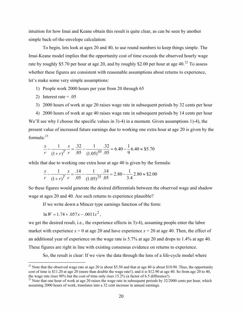
To begin, lets look at ages 20 and 40, to use round numbers to keep things simple. The

Imai-Keane model implies that the opportunity cost of time exceeds the observed hourly wage

rate by roughly $5.70 per hour at age 20, and by roughly $2.00 per hour at age 40.22 To assess

whether these figures are consistent with reasonable assumptions about returns to experience,

let’s make some very simple assumptions:

1) People work 2000 hours per year from 20 through 65

2) Interest rate = .05

3) 2000 hours of work at age 20 raises wage rate in subsequent periods by 32 cents per hour

4) 2000 hours of work at age 40 raises wage rate in subsequent periods by 14 cents per hour

We’ll see why I choose the specific values in 3)-4) in a moment. Given assumptions 1)-4), the

present value of increased future earnings due to working one extra hour at age 20 is given by the

formula:23

70.5$40.69140.6

05.32.

)05.1(1

05.32.

)1(1

45 ≈−=−=+

−rx

rrx

T

while that due to working one extra hour at age 40 is given by the formula:

00.2$80.24.3

180.205.14.

)05.1(1

05.14.

)1(1

25 ≈−=−=+

−rx

rrx

T

So these figures would generate the desired differentials between the observed wage and shadow

wage at ages 20 and 40. Are such returns to experience plausible?

If we write down a Mincer type earnings function of the form:

20011.057.74.1ln xxW −+= ,

we get the desired result, i.e., the experience effects in 3)-4), assuming people enter the labor

market with experience x = 0 at age 20 and have experience x = 20 at age 40. Then, the effect of

an additional year of experience on the wage rate is 5.7% at age 20 and drops to 1.4% at age 40.

These figures are right in line with existing consensus evidence on returns to experience.

So, the result is clear: If we view the data through the lens of a life-cycle model where 22 Note that the observed wage rate at age 20 is about $5.50 and that at age 40 is about $10.90. Thus, the opportunity cost of time is $11.20 at age 20 (more than double the wage rate!), and it is $12.90 at age 40. So from age 20 to 40, the wage rate rises 98% but the cost of time only rises 15.2% (a factor of 6.5 difference!). 23 Note that one hour of work at age 20 raises the wage rate in subsequent periods by 32/2000 cents per hour, which assuming 2000 hours of work, translates into a 32 cent increase in annual earnings.

20

work experience increases wages, then the inter-temporal elasticity of substitution has to be

roughly 2 to 3.24 Reasonable estimates of returns to experience imply that the shadow wage

increases by only about 15% from start to peak of the life-cycle wage-age profile, yet hours

increase by roughly 30% to 50% over the same period.25 So it is clear what “identifies” the

parameter η in the Imai-Keane structural model, even though there is no “instrument” or “natural

experiment” exploited in the estimation.26

This discussion also illustrates a more general point. Critics of structural work often

argue that we should just “let the data speak,” rather than imposing structure in estimation. Such

a statement is incomprehensible in the life-cycle labor supply context. That is, the inter-temporal

elasticity of substitution is not something we can “see” simply by looking at data – no matter

what sort of “ideal” variation the data might contain – because any calculation of η involves

intrinsically unobservable constructs, like the opportunity cost of time and the marginal utility of

wealth, that only exist in theory.

6. “Too Many Assumptions”

The most common criticism of structural econometric work is that it relies on “too many”

assumptions. In fact, I have often seen structural work dismissed out of hand for this reason. In

contrast, many believe “simple” empirical work is more “convincing.” I readily concede that the

typical structural estimation exercise relies on a long list of maintained a priori assumptions. But

we are kidding ourselves if we think “simple” estimators don’t rely on just as many assumptions.

As an illustration, let me return to the example of estimating effects of day care on child

outcomes from Section 4. Bernal (2007) structurally estimates a model of maternal work and

child-care use decisions that incorporates a child cognitive ability production function similar to

24 Of course, if we view the data through the lens of a different model, we can reach yet a different conclusion. For instance, we can reconcile a small value of η with the observed life-cycle paths of hours and wages if we dispense with rational expectations, and assume that workers don’t understand how much wages rise with work experience. 25 It is worth emphasizing that Imai and Keane (2004) ignore corner solutions (i.e., unemployed and out-of-the-labor force states). These are more common at younger ages, so ignoring them would lead one to understate the steepness of both the life-cycle hours and wage paths. Thus, it seems unlikely that allowing for corners would greatly alter conclusions about the inter-temporal elasticity of substitution. Imai and Keane also ignore aggregate shocks, treating the rental price of human capital and the interest rate as constant over time. As the life-cycle wage/hours patterns that identify the inter-temporal elasticity of substitution appear to be typical (i.e., not cohort or time period specific), it is difficult to see how a particular pattern of aggregate shocks or interest rate changes could drive the result. 26 It is interesting that Prescott’s (1986) long held position that the micro empirical work on estimating the inter-temporal elasticity of substitution must be flawed, because standard theory implied that η had to be at least 2 to rationalize the macro data, appears to be vindicated by this result.

21

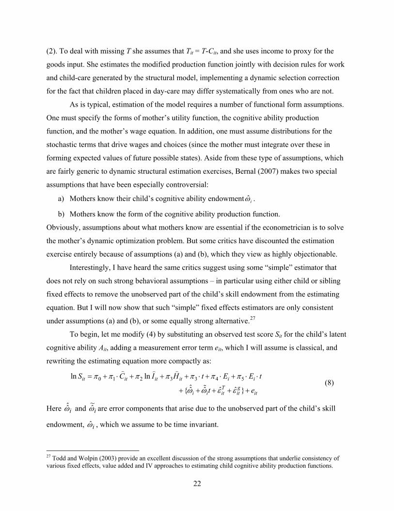
(2). To deal with missing T she assumes that Tit = T-Cit, and she uses income to proxy for the

goods input. She estimates the modified production function jointly with decision rules for work

and child-care generated by the structural model, implementing a dynamic selection correction

for the fact that children placed in day-care may differ systematically from ones who are not.

As is typical, estimation of the model requires a number of functional form assumptions.

One must specify the forms of mother’s utility function, the cognitive ability production

function, and the mother’s wage equation. In addition, one must assume distributions for the

stochastic terms that drive wages and choices (since the mother must integrate over these in

forming expected values of future possible states). Aside from these type of assumptions, which

are fairly generic to dynamic structural estimation exercises, Bernal (2007) makes two special

assumptions that have been especially controversial:

a) Mothers know their child’s cognitive ability endowment iω̂ .

b) Mothers know the form of the cognitive ability production function.

Obviously, assumptions about what mothers know are essential if the econometrician is to solve

the mother’s dynamic optimization problem. But some critics have discounted the estimation

exercise entirely because of assumptions (a) and (b), which they view as highly objectionable.

Interestingly, I have heard the same critics suggest using some “simple” estimator that

does not rely on such strong behavioral assumptions – in particular using either child or sibling

fixed effects to remove the unobserved part of the child’s skill endowment from the estimating

equation. But I will now show that such “simple” fixed effects estimators are only consistent

under assumptions (a) and (b), or some equally strong alternative.27

To begin, let me modify (4) by substituting an observed test score Sit for the child’s latent

cognitive ability Ait, adding a measurement error term eit, which I will assume is classical, and

rewriting the estimating equation more compactly as:

0 1 2 3 3 4 5ln lnˆ̂ ˆ ˆ ˆ{ }

it it it it i iT g

i i it it it

S C I H t E

t e

π π π π π π π

ω ω ε ε

= + ⋅ + + + ⋅ + ⋅ + ⋅ ⋅

+ + + + +

E t (8)

Here and iω̂̂ iω~̂

are error components that arise due to the unobserved part of the child’s skill

endowment, iω̂ , which we assume to be time invariant.

27 Todd and Wolpin (2003) provide an excellent discussion of the strong assumptions that underlie consistency of various fixed effects, value added and IV approaches to estimating child cognitive ability production functions.

22

The and are the mother’s tastes for time and goods inputs into child cognitive

production. These presumably have permanent components, arising from the mother’s tastes for

leisure and child quality, as well as transitory components, arising from shocks to offer wages,

shocks to employment status (e.g., layoffs), changes in day care availability, etc.. Clearly, the

transitory components of and are potentially correlated with the inputs

Titε̂ g

itε̂

Titε̂ g

itε̂ itC and itIln , a

problem that is not addressed by fixed effects, and that requires either use of instrumental

variables or joint estimation of the production function and the decision rules for the inputs. But

lets set that problem aside, and focus on the other assumptions required for fixed effects.

Much empirical work that relies on fixed effects techniques starts by writing down an

error components specification like (8). But this practice obscures the economic factors behind

the error components. From (4), we see that and iω̂̂ iω~̂

appear in the error term of (8) for two

reasons. First, because iω̂ enters the cognitive ability production function, and second, because it

enters the mother’s conditional decision rules for time and goods inputs. A child fixed effects

estimator, or, alternatively, first differencing (8), does not, in general, eliminate the error

component that arises because iω̂ enters these decision rules, because, to the extent that iω̂ alters

per-period inputs, its impact cumulates over time. We can avoid this problem by assuming either:

(a) mothers know nothing about the child’s cognitive ability endowment, or (b) mothers do know

something about the child’s endowment, but do not consider it when deciding on inputs.

On the other hand, suppose mothers do consider the child’s ability endowment when

making decisions about “quality” time and child care inputs. Consider first the case where

mothers know the ability endowment perfectly. In that case, fixed effects will not eliminate the

iω~̂

term in (8), but applying fixed effects to the differenced equation (or double differencing) will

do so. But, as noted by Blau (1999), existing data on test scores at pre-school ages almost never

contain three observations for a single child, so as a practical matter this is not feasible, and, even

if it were, efficiency loss would be a very serious problem.

Finally, consider the more difficult case where mothers have uncertainty about the child’s

true cognitive ability, and learn about it by observing test scores. In a learning model, a lower

than expected test score at age t-1 would cause the mother to update her perception of the child’s

ability, iω̂ . If iω̂ enters the decision rules for time and goods inputs, this would affect inputs

23

dated at time t. This violates the strict exogeneity assumption that underlies the fixed effects

estimator, so fixed effects is inconsistent.

For example, suppose a child has a surprisingly poor test score at t-1. To compensate, the

mother increases her own time input and reduces the day care time input between t-1 and t. This

induces negative correlation between a change in inputs itC - 1, −tiC and the differenced error (eit

– ei,t-1).28 It seems plausible that the effect of child-care time is biased in a negative direction.29

A similar problem arises in a model where mothers do not know the cognitive ability

production function. In that case, they may use child test outcomes to learn about the production

technology. Hence, for example, a child who was in full-time day care at age t-1 and who had a

poor test outcome might be removed from that setting, or have day-care time reduced. This again

induces a correlation between time t-1 test score realizations and time t inputs, violating the strict

exogeneity assumption. Here, the likely effect is to attenuate the estimated effects of the inputs.

Thus, we see that child fixed effects estimators implicitly assume either that mother’s do

not know child ability endowments, or, if they do know them, that they do not consider them

when making decisions about child-care and goods inputs, or, if they do know them and consider

them, that they know them perfectly (no learning), as well as knowing the production function.30

Furthermore, as noted earlier, consistency of fixed effects requires the strong assumption that the

taste shocks and do not affect input decisions. Clearly, the assumptions required for

consistency of “simple” fixed effects estimators are at least as strong as any in Bernal (2007).

Titε̂ g

itε̂31

28 Note that, in this example, we drive down ei,t-1, which drives up (eit – ei,t-1), and we drive down Cit. 29 As scores are measured with error, a surprisingly bad score at t-1 is likely part measurement error. Thus, it will tend to improve in the next period. Part of the improvement is falsely ascribed to the reduced child-care time input. 30 Similar problems arise with household fixed effects. Consistency requires that there are no sibling specific ability endowments, or, if there are, that mothers do not know them, or do not consider them when making decisions, or, if they do consider them, that they know them perfectly (no learning). With learning about ability or the production technology, outcomes for the first child affect input choice decisions for the second child, violating strict exogeneity. 31 Similar issues to those discussed here are addressed by Rosenzweig (1986) and Rosenzweig and Wolpin (1995) in the context of estimating birthweight production functions. Say we are interested in effects of inputs like maternal diet on a child’s birthweight. Problems arise if child endowments affect birthweight, and if maternal inputs are correlated with child endowments. Taking a sibling difference in birthweight outcomes can eliminate the mother specific (or common across siblings) part of the endowment, leaving only the child specific endowments. But the difference in maternal inputs between pregnancies may be endogenous, if, say, the birthweight outcome for the first child affects the mother’s behavior during the second pregnancy. But here, informational constraints imply a natural IV procedure, since the mother can’t know the first child’s specific endowment during the first pregnancy (i.e., it is only revealed when the child is born and birthweight observed). Thus, maternal inputs during the first pregnancy are uncorrelated with the child specific endowments. This suggests a FE-IV procedure, using maternal inputs during the first pregnancy to instrument for the difference in maternal inputs between the two pregnancies. Unfortunately, this sort of procedure does not work in cognitive ability production function case. That case is harder, because the mother can observe something about the first child’s cognitive ability when choosing inputs for the first child.

24

7. Un-Natural Non-Experiments and “Low-Grade Quasi-Experiments”

Rosenzweig and Wolpin (2000) report finding only five random outcomes arising from

natural mechanisms (e.g., weather events, twin births, realizations of child gender) that have

been used in the “natural experiment” literature as instruments. They refer to these events as

natural “natural experiments.” They list 20 papers that use these 5 instruments to estimate

“effects” of education and experience on earnings, “effects” of children on female labor supply,

and elasticities of consumption with respect to permanent and transitory income shocks. Given

the rarity of natural experiments that truly generate something resembling treatment and control

groups, the natural experiment literature would be a rather small one – except for the fact that

many researchers have been willing to seriously stretch the definition of a natural experiment. In

much of the literature, a “natural experiment” has come to mean any policy intervention that

affects two groups differently, regardless of whether those two groups look similar initially.

For example, in recent years I have seen (1) small firms used as a control group for large

firms, in estimating the effect of changes in credit laws that only affect large firms’ output, (2)

men used as a control group for women, in estimating the effect of changes in welfare rules

(affecting only women) on interstate migration, (3) upland counties in the deep South used as a

control group for coastal counties, to estimate the impact of treatment for helminth infection,

given only to residents the latter, on child outcomes,32 (4) people under 65 used as a control

group for people over 65 to estimate the effect of Medicare on mortality rates, etc..

Shadish, Cook and Campbell (2001) do not refer to such designs as “natural

experiments,” but rather, as “low-grade quasi-experiments.” And they note (p. 485), “As scholars

who have contributed to the institutionalization of the term quasi-experiment, we feel a lot of

ambivalence about our role.” They go on to note (p. 500) that “… the word quasi-experiment is

routinely used to justify causal inferences, even though designs so referred to are so primitive in

structure that causal conclusions are often problematic. We have to challenge such advocacy of

low-grade quasi-experiments …” and (p. 503) “… we want to draw attention again to a common

but unfortunate practice in many social sciences – to say that a quasi-experiment is being done in

order to provide justification that the resulting inference will be valid. Then a quasi-experimental

design is described that is so deficient in the desirable structural features … which promote

better inference, that it is probably not worth doing.”

32 The coastal counties were chosen for treatment precisely because they had much higher initial rates of infection.

25

There is now a large literature in economics applying “difference-in-difference” (DD)

estimators to so-called “natural experiments” in order to estimate “casual effects” of policy

interventions, but in many instances the designs should be called “low-grade quasi-experiments”

at best. I’ll use a simple example to illustrate this approach, and the strong implicit assumptions

on which it relies (Blundell and MaCurdy (1999) provide a good general discussion). The AFDC

program in the U.S. provided welfare benefits to single mothers with children under 18. One

aspect of the 1996 welfare reform, which replaced AFDC with TANF, was the implementation

of a 5-year time limit on welfare receipt.33 If women are forward looking, this creates an option

value to staying off welfare today, since this choice preserves eligibility for the future. Thus, we

might expect welfare participation to fall even before women run up against the limit. But,

ignoring fertility, this incentive can’t apply to women whose oldest child was at least 13 when

the limit was imposed, since their oldest child will reach 18 before they can use up their

eligibility. Thus, the argument goes, to estimate the effect of the time limit, we can use women

whose children were 13-17 when the 5-year limit was imposed are a control group, while women

with younger children are the treatment group.

This idea is illustrated in Table 2, Panel A, which is adapted from Grogger (2004). In the

before vs. after time limit comparison, the welfare participation rate for single mothers with

youngest children in the 13-17 year age range drops from 16% to 11%. Since these women were

not affected by the time limit, this drop is attributable entirely to other time-varying factors (i.e.,

other aspects of the welfare reform, or changes in the macro economy). This gives 5 percentage

points as our estimate of the impact of all these other factors.

Next, consider single mothers with youngest children in the 0-6 year age range. They are

impacted by time limits, since they could use up 5 years of benefits long before their children

reach age 18. Welfare participation dropped 17.5 percentage points among this group. Thus,

using the DD approach, we attribute 5 percentage points of this drop to “other factors,” leaving

12.5 percentage points as the drop attributable to time limits. This is a very large effect, implying

71% of the drop in welfare among single mothers with young children was due to time limits.

As Grogger (2004) points out, this estimate relies on a number of strong assumptions.

Most critically, it supposes that all the “other factors” have the same impact on mothers with old

33 This is actually a gross oversimplification made for purposes of exposition. I urge the interested reader to refer to Fang and Keane (2004) for details of how these limits were implemented, along with evidence that they were rarely imposed strictly. That paper also discusses the problems with DD estimators in this context in more detail.

26

vs. young children. This is a very strong assumption, since mothers with young vs. old children

differ in important ways. To see this, note that Table 2 also shows that welfare participation rates

are much higher among single mothers who have young children (41%) than among single

mothers who have older children (16%). This illustrates the dramatic difference between the two

groups, and calls into serious question the assumption that they would be impacted in the same

way by other aspects of welfare reform or by the business cycle.

Furthermore, the fact that the baseline participation rates differ so greatly between the

two groups creates a second serious problem for the simple DD approach. Even if it were true

that unmeasured time varying factors have a common impact on each group, to use DD we need

to know if the “common impact” applies when we measure impacts in levels, or percentages, or

by some other metric. This point is also illustrated in Table 1. The last column shows percentage

changes in participation rates for each group. The single mothers with older children had a 31%

decline in welfare participation, while those with young children had a 42% decline. So, if

unmeasured factors have a common effect in percentages, the DD estimate of the effect of time

limits is -11%. This corresponds to only 4.6 percentage points, which is about a third as large as

the 12.5 point effect we obtained using the DD-levels estimator. Thus, time limits seem much

less important when we measure impacts in percentages rather than levels.

The problem is obvious, but often glossed over in the natural experiment literature.34 An

exception is Meyer, Viscusi and Durbin (1995), who use low-wage workers as a control group

for high-wage workers to estimate the effect of an increase in disability benefits, affecting only

high earners, on weeks receiving disability. Before the program, mean weeks differed greatly for

the two groups (11.2 for high earners, 6.3 for low earners). The DD-levels estimate implies a

negative program effect on weeks of disability, while DD-percentages implies a positive impact.

To deal with this sort of problem, Athey and Imbens (2002) have proposed an alternative

approach to DD estimation that does not require one to specify the transformation of the

dependent variable. Their approach can be thought of as re-weighting the control group sample,

so the control group outcome distribution is identical to that of the treatment group at baseline.35

The re-weighted control group outcome distribution in the post-treatment period then provides an

34 As an example, see Stock and Watson (2003) Figure 11.1 in chapter 11 on “experiments and “quasi-experiments,” and the surrounding discussion, which states that the DD estimator can eliminate bias that arises when treatment and control groups differ. 35 I am interpreting their procedure as importance sampling, with the controls providing the “source” distribution, and the counterfactual distribution for the treated (given they receive no treatment) being the “target.”

27

estimate of the impact of all the “other” factors on the treatment group.36

I implement this approach for the time limit example in Panel B of Table 2. Note that

31% of the control group leaves welfare due to “other” factors. Hence, in the weighted control

group, we have (1-.69)⋅41.3%=28.4% on welfare in the post-reform period. Thus, the estimate of

the effect of time limits on the treated is 23.8-28.4=-4.6 points, which corresponds to -11.1%. It

is no coincidence that this is the same as the DD-percentages estimate in Panel A. In the binary

discrete outcome case, the Athey-Imbens estimator reduces to exactly the DD-percentage

estimator.37 That is, it reduces to assuming that percentage changes are the right metric for

measuring the impact of "other time varying factors."

In summary, the Athey-Imbens approach of re-weighting the control group to resemble

the treatment group makes perfect sense when the two groups are basically “similar” – in the

sense that they contain identical types of agents, but where the type proportions simply differ

across groups (perhaps due to imperfection in random assignment). An example might be an

experiment that imposed time limits in some counties of a State but not others, and where

baseline welfare participation was higher in the “treatment” counties because they had a greater

representation of women with lower welfare “stigma.” Re-weighting then simply adjusts the type

proportions. But the Athey-Imbens approach does not help if the treatment and control groups

are fundamentally different, as in the high vs. low-wage worker or young vs. older children

examples. There is no obvious economic reason why the percentage change is the “right” metric

to measure impact of “other factors” in such cases.

Thus, there is no way around the problem of dissimilar treatment and control groups

other than to make extensive use of theory. That is, we have to do the hard work of measuring

the important “other” factors that may have differentially affected people with different

characteristics over the sample period, and we need to make a priori theoretical assumptions

about how these “other” factors differentially affect different groups. The DD approach is not a

panacea that allows us to deal with unmeasured time varying factors in an atheoretic way.

36 The re-weighted control group provides the correct counterfactual distribution for the treated (given no treatment) under Athey and Imbens’ weak monotonicity and conditional independence assumptions 4.1 and 4.2. These essentially mean that, if D denotes the discrete outcome, then a policy that reduces P(D=1) shifts people from D=1 to D=0 but not vice versa. It is worth noting that Athey and Imbens are very up front about this being a strong assumption (e.g., I’ve already noted that this assumption may be violated in the draft lottery/schooling example). 37 Note: If we call D the discrete outcome, and P(D=1) goes down in the control group, then their estimator is the percentage change in P(D=1) in the treatment group minus that in the control group. But, if P(D=1) goes up, their estimator is the percentage change in P(D=0) in the treatment group minus that in the control group.

28

8. Has Atheoretic Work Led to Progress in Other Disciplines?

One argument for an atheoretic, “let the data speak,” empiricist approach is that we must

understand and catalogue a whole range of “facts” or empirical regularities before we can

construct useful theories. I suspect this is what Angrist and Krueger (1999) have in mind when

they present the quote from Sherlock Holmes: “It is a capital offense to theorize before all the

facts are in.” (emphasis added). In contrast to this “empiricist” approach, the structural approach

is viewed as imposing a priori theory on the data, preventing us from hearing what it has to say.

Notably, this empiricist perspective is inconsistent with the views of most researchers in

the history of science who study how scientific progress is actually made across a wide range of

fields. For instance, Kuhn (1962) asserts there are “three normal foci for scientific investigation,”

which he lists as (i) “facts that the paradigm has shown to be important,” (ii) “facts that can be

compared directly with the predictions of the paradigm theory,” and (iii) “empirical work

undertaken to articulate the paradigm theory,” including determination of universal constants and

universal laws (e.g., Boyle’s Law, Coulomb’s Law, etc.). Kuhn goes on to note: “Perhaps it is

not apparent that a paradigm is a prerequisite to the discovery of laws like these. We often hear

that they are found by examining measurements undertaken for their own sake and without

theoretical commitment. But history offers no support for so excessively Baconian a method.”

A good example of what Kuhn is talking about here is provided by the history of

mechanics. This is often presented as if Galileo did experiments to measure rates of acceleration

of falling objects simply out of interest. Then Newton comes along, takes the first two laws of

motion “discovered” by Galileo, along with the celestial laws of motion “discovered” by Kepler,

and from them develops de novo a unified theory of gravity. This distorted history ignores the

fact that Galileo did not decide to roll balls down inclined planes simply out of some general

curiosity. His experiments were motivated by a theoretical framework that he already had in

mind, in which acceleration is zero when an object moves in parallel to the earth, and constant

when an object moves vertically.38 Galileo ran the experiments to see if his theoretical

predictions would be born out. Only under his two assumptions about acceleration can one even

think of measuring the rate of acceleration in vertical free fall by rolling balls down an inclined

38 Also widely forgotten is that the Aristotelian model of velocity proportional to force had been widely rejected centuries earlier. Galileo’s theory built on earlier work by such men as Philiponus (6th century) and Burdian (14th century), who rejected Aristotle by viewing impetus as permanent, thus anticipating inertia, and Heytesbury and Orsem (14th century), who developed the “Merton rule” of uniformly accelerated motion.

29

plane. Similarly, Kepler believed in the heliocentric system a priori.39

Returning to the quote from Conan Doyle, it is interesting that Einstein and Infeld (1938),

in their history of modern physics, also suggest an analogy of the scientist with the great

detective, who “… after gathering the requisite facts, finds the right solution by pure thinking.”

But they go on to say: “In one essential this comparison must be regarded as highly superficial.

Both in life and in detective novels the crime is given. The detective must look for letters,

fingerprints, bullets, guns, but at least he knows that a murder has been committed. This is not so

for a scientist. … The scientist must commit his own crime, as well as carry out the

investigation.” Thus, regarding key experiments in the history of physics, Einstein and Infeld

argue “it is hardly possible to imagine such experiments performed as accidental play, without

pre-existence of more or less definite ideas about their meaning.”

In summary, I would agree with these authors that we cannot even begin the systematic

assembly of facts and empirical regularities without a preexisting theoretical framework that

gives the facts meaning, and tells us which facts we should establish. The structural approach of

viewing the data through an organizing theory is perfectly consistent with the approach that is

standard and has generated success in other sciences, while an atheoretic approach is not.40

9. Estimating Structural Models vs. Other Scientific Activities

As I’ve described, the goal of structural econometric work is to estimate fully articulated

models (e.g., an estimable life-cycle labor supply model), or else to estimate key parameters of

economic models (e.g., the inter-temporal elasticity of substitution parameter). These activities

both fall within Kuhn’s third “focus” of scientific investigation, which he calls “empirical work

undertaken to articulate the paradigm theory.” I think that failure to clearly understand this has

been a source of great confusion, both between structural econometricians and researchers who

pursue other types of empirical work, and within the structural econometric community itself.

The first important thing to note is that being an advocate of structural econometrics does

39 It is now largely forgotten that the empirical evidence at the time actually provided strong support for a geocentric view. Tycho Brahe was unable to find any evidence of stellar parallax despite painstaking attempts, and instruments accurate enough to detect it were not developed until the mid-1800s. 40 Interestingly, even leading experimental methodologists consent to this view. As Shadish, Cook and Campbell (2001), p. 27, state “The logical positivists hoped to achieve foundations on which to build knowledge by tying all theory tightly to theory free observation … but this … failed to recognize that all observations are impregnated with substantive and methodological theory, making it impossible to conduct theory free tests,” and (p. 29) “The experiment is not a clear window that reveals nature directly to us. To the contrary, experiments yield hypothetical and fallible knowledge that is often dependent on context and imbued with many unstated theoretical assumptions.”

30

not mean that one is opposed to empirical investigators that fall into Kuhn’s first category, the

development of (i) “facts that the paradigm has shown to be important.” The first category

includes descriptive empirical work, as well as primary data collection, provided these efforts are

guided by a theoretical framework. In fact, they almost always are. Questions on surveys like the

PSID, NLS and HRS are not chosen randomly out of some universe of possible questions we

might ask, but are chosen carefully to measure quantities that certain theoretical frameworks, like

the life-cycle human capital model, tell us are important. People like Ken Wolpin, Chuck Manski

and Bob Willis have done a lot of work in recent years to help improve how well these surveys

measure key constructs of our paradigm theories.

Being an advocate of structural econometrics also does not mean that one is opposed to

empirical investigations that fall within Kuhn’s second category, the development of (ii) “facts

that can be compared directly with the predictions of the paradigm theory.” In fact, I think that

the best work in the “experimentalist” school can be thought of as falling within this category.

True natural experiments, as well as the un-natural quasi-experiments induced by changes in

policy that affect some groups but not others, provide us with excellent opportunities to validate

our models by confronting them with data. The key point, however, is that we should not be

content to catalogue what happened in such events (i.e., the “treatment effects”), but rather, we

must study whether our models can successfully predict what happened.

A good example is the work by Card and Krueger (1994), Neumark and Wascher (1995),

and Deere, Murphy and Welch (1995) on effects of the sharp increases in the national minimum

wage from $3.35 on March 31, 1990 to $4.25 on April 1, 1991, and the New Jersey specific

increase to $5.05 on April 1, 1992. These quasi-experiments provide important evidence that

may help distinguish among competing labor market theories. But progress can only be made if

one attempts to interpret the DD estimates of these authors in light of standard theories of labor

market equilibrium, such as the search and matching model of Burdett and Mortensen (1989), as

well as bringing more data to bear to help resolve some of the ambiguities of the original

studies41 - instead of taking the destructive tack of simply concluding the data refutes the law of

demand and stopping at that. Attempts by Flinn (2006) and Ahn, Arcidiacono and Wessels

(2007) to rationalize data on minimum wage effects in terms of search models appear promising.

41 Obviously, referring back to the discussion of DD in section 6, this also involves modeling the “other factors” that might have differentially affected the non-randomly selected treatment and control groups in these studies.

31

10. The Importance of Model Validation and Paradigm Development

Given that a priori assumptions are indispensable in interpreting data, I would argue that

structural econometricians should be less apologetic about the need to make assumptions (often

many assumptions!) in order to develop estimable structural models. Of course, one is entitled to

discount results from a model that, one feels, relies on “incredible” assumptions that may clearly

drive the results. For example, I personally would not believe estimates of returns to schooling

from models that assumed homogenous skill endowments, or of the extent of habit persistence in

choice behavior from models that assume homogenous tastes for product attributes.

But such “incredible” assumptions are not really the issue. The typical well-executed

structural estimation exercise presents a model based on a long list of assumptions, some of

which seem plausible but debatable, some of which seem difficult to evaluate on a priori

grounds, and some of which seem obviously false. Often, it is not clear if the obviously false

assumptions are innocuous simplifications or whether they might have a major impact on the

behavior of the model. How seriously should we take the exercise?42

In my view, determinations of the usefulness of such “well-executed” structural models –

both as interpreters of existing data and vehicles for predicting the impact of policy interventions

or changes in the forcing variables – should rest primarily on how well the model performs in

validation exercises. By this I mean: (1) Does the model do a reasonable job of fitting important

dimensions of the historical data on which it was fit? (2) Does the model do a reasonable job at

out-of-sample prediction – especially when used to predict the impact of policy changes that alter

the economic environment in some fundamental way from that which generated the data used in

estimation?

My use of the word “reasonable” here is unapologetically vague. I believe that whether a

model passes these criteria is an intrinsically subjective judgment, for which formal statistical

testing provides little guidance. This perspective is consistent with how other sciences treat

validation. Unfortunately, many economists have an idealized view of the “hard” sciences in

which models are maintained as long as they explain all observed data, and, when an experiment

or observation comes along that a model can’t explain, the model is immediately rejected. In

fact, this is far from the case; even in the “hard” sciences, validation is highly subjective.

42 Clearly, it is a serious error to reject a model as “not useful” simply because its assumptions are literally false. Good examples are the “large signal” and “small signal” models of transistors (see Fonstad, 1994). Both over-simplify the underlying physics, but each can accurately predict transistor behavior within a certain frequency range.

32

As Kuhn (1962) describes, models typically receive broad acceptance within a scientific

field because they explain better than other models certain observations which the members of

the field regard as key. Subsequently, a great deal of “mopping up” work is done to try to fit the

model to many other observations, or resolve its failures to do so. A model’s inability to explain

all aspects of the observed data is typically treated as a problem to be worked out over time via

gradual refinement, not a reason to reject the model per se.

As a concrete example, consider the life-cycle human capital investment model of Becker

(1967), Mincer (1958) and Ben-Porath (1967). Keane and Wolpin (1997) showed that a standard

version of this model provides a poor fit to observed data on education, employment and wages.

A key prediction of the framework is that schooling is concentrated at the start of the life-cycle.

The standard model generates this pattern qualitatively, but the quantitative prediction is poor.

The basic problem is that, given observed variability in wages, it is hard to get forward looking

agents to concentrate schooling at the beginning of life to the extent they do. Observed wages are

quite variable, so why not return to school whenever the offer wage draw is sufficiently low?

But, by adding a number of extra features that are not essential to the model, but that

seem reasonable (like costs of returning to school, age effects in tastes for schooling,

measurement error in wages, and so on), we were able to achieve what we regard as an excellent

fit to the key quantitative features of the data – although formal statistical tests still rejected the

hypothesis that the model is the “true” data generating process (DGP). Despite these problems,

there is nothing to indicate that the profession might be ready to drop the human capital

investment model as a framework for explaining school and work choices over the life-cycle.

Indeed, if we view the data through the lens of the life-cycle labor supply/human capital

investment model, a lot of empirical observations seem to make sense and hang together nicely.

For instance Keane and Wolpin (2000) show that, in such a model, differences in schooling and

labor supply between young black and white men can be largely explained based on the

differences in their skill endowments at age 16 plus labor market discrimination. That is, the

much lower educational attainment of young black men can be explained as a rational response

of forward looking agents to the constraints they face. We do not need to resort to various

alternative explanations like “excessive” present orientation and so on.

Similarly, work in the dynamic life-cycle framework by Cameron and Heckman (1998)

and Keane and Wolpin (2000, 2001) has shown that, viewed through the lens of this framework,

33

the wide differences in educational attainment across youth from different family backgrounds

can be almost completely explained by the differences in skill endowments that youth possess at

age 16. One need not resort to liquidity constraints, or stories like failure to understand returns to

college, to explain the lower schooling of youth from poor backgrounds.

Furthermore, Keane and Wolpin (2001) show that a life-cycle labor supply/ human

capital model can match cross-sectional asset distributions by age, and generate tuition effects on

college attendance that are similar to a wide range of estimates in the education literature, both in

the aggregate and broken down by parental background. Arcidiacono (2005) shows that the life-

cycle framework can explain decisions about college attendance and choice of major, as well as

wages conditional on major, using values for returns to experience and the importance of skill

“endowments” (prior to college) that are similar to those in Keane and Wolpin (2001). And Imai

and Keane (2004) use the life-cycle human capital framework to explain life-cycle patterns of

wages, hours and assets, using a value for the inter-temporal elasticity of substitution in labor

supply consistent with a wide range of macro evidence (see Prescott (1986)).

Thus, structural models in the life-cycle labor supply/human capital framework pass one

test of usefulness: they can coherently explain a wide range of key observations about wages,

educational choices, demographic and racial differences in behavior, etc.. They have also proven

useful because the results of Cameron-Heckman and Keane-Wolpin on the crucial importance of

age 16 skill endowments have focused attention on the need to get inside the black box of how

these endowments are determined. This is beginning to generate structural work within the

human capital paradigm on early childhood investments, thus further elucidating the paradigm.

This brings me to the second aspect of validation: out-of-sample prediction, especially

attempts to predict the impact of policy changes (or quasi-experiments) that change the economic

environment in an important way. I already discussed the point that a structural model can be

literally rejected as the “true” data generating process – which is not surprising since the model is

a simplification of reality – yet still be useful for organizing our view of a wide range of

phenomena. Similarly, a model that is literally false may still be useful for prediction. But how

can we develop confidence that a structural model is useful for policy prediction?

Again, as formal statistical tests of whether a model is the “true” DGP provide little

guidance, the question of usefulness is intrinsically subjective. Indeed, what gives me confidence

in a model may not give you confidence. Hence, the best I can do is to describe the process that I

34

have actually pursued (often in joint work with Ken Wolpin) in attempting to validate models.

I think our approach can be interpreted as a Bayesian updating process. We start with a

prior on how likely a model is to make accurate predictions about effects of certain types of

policy interventions. This influences our initial choices about details of model specification. For

example, in developing life-cycle models for men, with a goal of being able to explain college

attendance and responses to tuition subsidies and college loans, we might think incorporating

marriage, or couples’ fertility decisions within marriage, is not very important. In contrast, we

might think that life-cycle models of women that ignore marriage and fertility are unlikely to be

useful for prediction. Clearly, these are a priori judgments, and others may disagree.

Given a model, and upon seeing its fit to the historical data, we update our prior about its

usefulness. Personally, unless a model provides a reasonably good fit to the historical data, I

would have little confidence in its ability to predict results of policy interventions. However,

what constitutes a “reasonable” fit is clearly subjective. As I noted above, our standard is

certainly not the “objective” one that the model not be rejected by formal statistical specification

tests, because we expect structural models to be rejected by such tests (given enough data).

Finally comes the crucial step, which is to use the model in a range of policy prediction

exercises, and evaluate the accuracy of its predictions. But here we run into a key difficulty.

Policy changes that can be used to evaluate predictive ability of our models are actually rather

rare.43 Not only must a policy change occur, but, more challenging, data from before and after

the change must be available. Unlike engineering and, in some cases, the physical sciences, we

cannot typically run experiments designed to test our models.

Nevertheless, the best opportunity to test the predictive ability of structural models is to

attempt to predict the outcomes of those quasi-experiments that the world does present to us.

Again, I view this as a Bayesian updating process. After seeing how well a model does in such a

prediction exercise, we update our priors about the model’s usefulness. Clearly, this is an

ongoing process, where we gain or lose confidence in models over time, perhaps at some point

deciding to repair or abandon them.44

Still, given the rarity of such events, it seems essential to develop other ways to validate

43 A search of the structural estimation literature reveals few attempts to validate structural models using quasi-experiments. For references, see Keane and Wolpin (1997, 2005) and Wolpin (1996). Attempts to validate reduced form or statistical models, or even estimates of causal effects derived from “natural experiments,” are also rare. 44 I expect that such a process will only in rare instances lead to complete rejection of models. Rather it may lead to refinement of our notions of the contexts where the model does and does not perform well.

35

structural models. Keane and Wolpin (2007) suggest two such strategies. One is to split the

historical data into subsets that were subject to different policy regimes, estimate a model on one

subset, and make predictions for the other. The other is to make forecasts of hypothetical policy

interventions, where we have strong priors on how the response should look. We illustrate these

ideas using a model of life-cycle labor supply, human capital investment, marriage and fertility

decisions of women. This model, which extends earlier work for men (i.e., Keane and Wolpin

(1997, 2000, 2001)), performs rather well, in our judgment, in these validation exercises.45

Finally, it is important to stress the subjective nature of any single validation exercise. A

prediction may be viewed as “reasonably” accurate by one observer but not another. And, given

the same validation exercise, one observer may view success in the exercise as highly persuasive

regarding the model’s ability to make accurate predictions in other contexts, while another may

not. Nevertheless, via multiple validation exercises, it may be possible to approach consensus.

11. Alternative Approaches to Validation

Besides predictive tests, another approach to model validation is to collect or obtain

additional data that can be used to test or estimate certain key predictions, key mechanisms or

key individual equations or parameters of the model. For example, the model of life-cycle

investment in health by Khwaja (2005) predicts that subsidized insurance would not encourage

unhealthy behaviors. This is because, in his dynamic model, the usual moral hazard effect that

arises in a static model is counteracted by a horizon effect – better health insurance increases life

expectancy, which increases the return to investment in good health. But life expectancy is not

observed in the data used to estimate the model. In principle, the mechanism of the model could

be tested by gathering data on life expectancy and looking at its effect, ceteris paribus, on health

investment. Of course, this is an extremely difficult exercise, because it requires that one find an

instrument that exogenously shifts life expectancy (i.e., that is uncorrelated with unobservables

that shift investment in health, such as unmeasured aspects of health or tastes for health).46

45 We also found that simple “statistical” models (i.e., logits for welfare and work using the state variables as covariates), which fit in-sample data at least as well as the structural model, did not pass this test. This led us to conclude that these models are not useful for prediction. This illustrates how theory can aid prediction. 46 As another example, the model in Keane and Wolpin (2001) predicts that more generous student loan programs have little effect on college attendance. Instead, they primarily affect consumption, work and borrowing/transfers from parents while in school. But they do not directly observe parental transfers in their data (only inferring them from changes in assets). One could in principle gather data on transfers from parents under different student loan regimes to test this prediction.

36

Similarly, we might attempt to estimate individual key equations or parameters of a

model in ways that do not rely on the full set of assumptions that are required for full information

maximum likelihood (FIML) estimation of the complete model. A finding that estimates are

similar when these alternative approaches are used would give us more confidence in the

specification of the structural model. This idea is related to the idea that, in some cases, certain

parameters of structural models can be shown to be semi-parametrically identified – that is, they

are identified in a technical sense without the need for the full set of assumptions required for

FIML estimation of the complete model.

It should be stressed however, that this “piecemeal” approach to estimating parts of

complete models is fraught with danger for the unwary. One must be careful that one’s approach

to estimating some subset of parameters of a structural model is consistent with the structure of

the model. A classic example of confusion on this point is the attempt to use micro-data evidence

to validate the choice of the inter-temporal elasticity of substitution parameter in real business

cycle models. The macro models required an estimate of the elasticity with respect to the

opportunity cost of time, while the micro data studies were not designed in such a way as to

deliver that parameter (except under rigid assumptions about human capital).

Another example is the attempt to use “simple” estimators to estimate “returns” to

schooling or experience, or to estimate “effects” of inputs on child production. As Rosenzweig

and Wolpin (2000) discuss, such estimates are not generally interpretable as structural

parameters of human capital or cognitive ability production functions. In fact, as I stressed in

Sections 3-7, “simple” estimators for single equations or individual parameters of structural

models typically rely on strong implicit assumptions. Estimation of a single equation in a way

consistent with the overall model may require that the equation be estimated jointly with

approximations to the decision rules generated by the complete model – which is the point of

Heckman (1974) – or, at least, that instruments be chosen with careful guidance from theory.

12. Identification vs. Validation

The literature on semi-parametric identification of structural model parameters seems to

be motivated by the following notion: if it can be shown that certain key parameters of a

structural model are identified even if the functional form assumptions required for FIML

estimation are relaxed, then we gain confidence that the model is a useful tool for organizing the

37

world and making predictions. In other words, there is a general notion that we can have more

confidence in a particular parameter estimate – say, e.g., the coefficient on education in a human

capital production function – if that parameter is estimated with as little auxillary structure as

possible. This view seems to be widely accepted among applied researchers.

This line of argument poses an important challenge to the structural econometric research

program, because construction of formal semi-parametric identification arguments for structural

models is typically only possible for very simple, stylized models that are not rich enough to

provide a reasonable fit to data. In contrast, rich structural models that can provide a good fit to

data typically involve many maintained assumptions whose role in identification may be difficult

to assess. In this situation, the proper response is to stress the crucial role of model validation.

Indeed, I would argue a certain primacy for validation exercises over identification analysis for

purposes of building confidence in models.

That is, regardless of how plausible the source of identification for a parameter may seem

to be, I would not have great confidence in the estimate until it was shown that, when placed

within a complete structural model, that model gives a reasonable fit to observed data and

forecasts well. To give a concrete example, Ashenfelter and Krueger (1994) estimate the return

to schooling as roughly .12, using a simple procedure that many regard as giving a credible

estimate that does not rely on many auxiliary assumptions. Of course, this is controversial, and

many (including myself) would argue that the estimate is based on strong implicit assumptions.

But let me put that aside for now and take it for granted that the .12 is a “robust” estimate. I

personally do not find that figure credible, because, in my view, it is difficult to construct a

plausible model of behavior where the return to schooling is so high, yet people choose to get as

little a schooling as they do.47

In contrast, suppose the schooling coefficient were estimated in the context of a fully

specified structural model using FIML, and this model performs well in validation exercises (i.e.,

it fits the data well and forecasts well). Then, we at least know that there exists a reasonable

looking model that can rationalize observed behavior using such a value for the schooling

parameter. Hence, I would have more confidence in the structurally estimated parameter than in

47 Of course, if one looks at schooling choice data alone, one can rationalize a low rate of school attendance with a very high return to schooling simply by assuming that the (psychic) cost of schooling is great enough. However, in a model that attempts to fit both choices and wages, raising both the cost and return to schooling so as to hold the attendance rate fixed will simultaneously raise the observed wage premium for highly educated workers over uneducated workers. The difficultly comes in fitting both dimensions of the data simultaneously.

38

the “robust” estimate. Indeed, as noted in the review by Belzil (2007), structural estimates of

returns to schooling are generally lower than “simple” IV estimates.48 This is precisely because

the latter tend to be too high to rationalize schooling choice in a life-cycle framework.

13. Where Structural Econometricians Need to Do Better

In my view there is another reason that structural econometric work fell out of fashion,

and here the fault lies with the structural econometricans themselves. Historically, structural

econometric work tended to pay little attention to the issue of model validation. It has often been

treated as a feat worthy of praise to simply estimate a structural model, regardless of whether the

model can be shown to provide a good fit to the data, or perform well in out-of-sample predictive

exercises. I see no reason why an estimated structural model should move my priors about, say,

the likely impact of a policy intervention, if it fits the in-sample data poorly and/or has not been

shown to perform reasonably well in any validation exercises. Structural econometricians need to

do a much better job in this area in order for structural work to gain wider acceptance. I do think

that in recent years our performance in this area has improved considerably.

Historically, a closely related problem is that estimation of structural models is so

technically difficult that, in the mid to late 80s, only very stylized models could be estimated.

These models were of necessity too sparse to have any hope of providing a reasonable fit to the

data. But advances in computation, and the development of simulation-based inference in the late

80s and early 90s, now allow us to estimate much richer structural models than would have been

imaginable 10 years ago. For instance, it is now possible to accommodate rich patterns of

preference heterogeneity, whereas this was not possible before. It was this prospect that

convinced me to start working on structural models in the early 90s. But the perceptions of the

profession as a whole about what is feasible in structural modeling have lagged behind the

current frontier. For instance, Angrist and Krueger (1999) state “we ignore structural modeling

since that topic is well covered elsewhere,” and then reference a survey dated 1986.

14. Conclusion

In the preface to Fear and Trembling, Kierkegaard (1983) states, “Not only in the 48 As noted by Belzil (2007) structural estimates of the schooling coefficient in a Mincer type earnings equation are typically in the .05 to .08 range. For example, Keane and Wolpin (2001) obtain an estimate of .075, in a model that allows for liquidity constraints (which are often invoked as way to rationalize co-existence of high expected returns with relatively low attendance rates).

39

business world, but also in the world of ideas, our age stages a real sale.” He is referring to the

notion that knowledge can be obtained “cheaply.” Kierkegaard means “cheap” in both a

psychological and an epistemological sense: (1) knowledge is “cheap” in the sense we don’t have

to work too hard to get it, and (2) knowledge is “cheap” in the sense that there exists a process or

system for accessing objective or absolute truth. The former statement can be viewed as a

critique of the sociology of academia, while the later can be viewed as an attack on the Hegelian

system, in favor of Kierkegaard’s subjectivism.

Kierkegaard’s critique of academic philosophy in the Europe of the mid-1800’s has

interesting implications for recent trends in empirical work in economics. It is fair to say that

“structural econometrics” has fallen out of fashion in the past 15 years, while “simple” empirical

approaches that eschew sophisticated statistical and theoretical modeling – “just letting the data

speak” – are in vogue. In my view, two of the primary reasons for this phenomenon are exactly

those that Kierkegaard identified. First, structural econometric work is just very hard to do,

simply in terms of the amount of labor involved. It often takes several years to write just one

good paper in this genre, and this poses a daunting prospect for the young assistant professor

seeking tenure, or the graduate student seeking to finish a dissertation. Using “simple” methods,

one can write papers quicker.

Second, there is a widespread belief that structural econometric modeling relies on strong

a priori statistical and economic assumptions – which is true! – while the alternative “simple”

approaches, such as “natural experiments,” enable us to obtain knowledge that is not conditional

on strong a priori assumptions. Unfortunately, this is not true, but in “our age” this problem

seems to be little appreciated.

We always need a priori identifying assumptions in order to learn anything of interest

from data, beyond perhaps the simplest of descriptive statistics. Data cannot simply “speak” and

reveal interesting aspects of economic behavior to an investigator whose mind is a blank slate,

devoid of economic priors. Structural econometric work does not rely on more assumptions than

“simple” atheoretic approaches. The only difference is that the assumptions are made explicit in

the structural approach. This makes the estimates interpretable, which is a prerequisite for

scientific progress. The “simple” path that eschews theory as the basis for empirical work has

almost never led to scientific progress in the past, and it is unlikely to lead to progress in the

future.

40

Acknowledgements: This paper was prepared as the keynote address at the Conference on Structural Models in Labor, Aging and Health held at Duke University on September 17-19, 2005. Conversations with Ken Wolpin were extremely valuable in developing some of the arguments presented here. Jim Heckman, Han Hong, Ed Vytlacil and a referee also provided helpful comments. I wish to thank these commentators without necessarily implicating them in the views expressed. Australian Research Council grants FF0561843 and DP0774247 have supported this research.

References Ahn, T., Arcidiacono, P. and W. Wessels, 2007, The distributional impacts of minimum wage increases when both labor supply and labor demand are endogenous. Working paper, Duke University. Altug, S. and R. Miller, 1989, Household choices in equilibrium. Econometrica 58, 543-570. Angrist, J., 1990, Lifetime earnings and the Vietnam era draft lottery: Evidence from Social Security administrative records. American Economic Review 80, 313-336. Angrist, J., 1995, Introduction to the JBES symposium on program and policy evaluation. Journal of Business and Economic Statistics 13, 133-136. Angrist, J. and A. Krueger, 1999, Empirical strategies in labor economics, in: O. Ashenfelter and D. Card, (Eds.), Handbook of labor economics, Vol. 3A. North-Holland, Amsterdam, pp.1277-1366. Arcidiacono, P., 2005, Affirmative action in higher education: How do admission and financial aid rules affect future earnings? Econometrica 73, 1477-1524. Ashenfelter, O. and A. Krueger, 1994, Estimates of the economic return to schooling from a new sample of twins. American Economic Review 84, 1157-73. Athey, S. and G. Imbens, 2002, Identification and inference in nonlinear difference-in-difference models. NBER technical working paper #280. Becker, G., 1967, Human Capital. Columbia University Press, New York. Belzil, C., 2007, The return to schooling in structural dynamic models: A survey. European Economic Review 51, 1059-1105. Ben-Porath, Y., 1967, The production of human capital and labor supply: A synthesis. Journal of Political Economy 75, 352-365. Bernal, R., 2007, The effect of maternal employment and child care on children’s cognitive development. International Economic Review, forthcoming.

41

Bernal, R. and M. Keane, 2007, Child care choices and children’s cognitive achievement: The Case of Single Mothers. Universidad de los Andes, working paper. Bjorklund, A. and R. Moffitt, 1987, Estimation of wage gains and welfare gains in self-selection models. Review of Economics and Statistics 69, 42-49. Blau, D., 1999, The effect of child care characteristics on child development. The Journal of Human Resources 34, 786-822. Blundell, R. and T. MaCurdy, 1999, Labor supply: A review of alternative approaches, in: O. Ashenfelter and D. Card, (Eds.), Handbook of Labor Economics, Vol. 3A. North-Holland, Amsterdam, pp. 1559-1695. Burdett, K. and D. Mortensen, 1998, Wage differentials, employer size and unemployment. International Economic Review 39, 257-273. Cameron, S. and J. Heckman, 1998, Life-cycle schooling and dynamic selection bias: Models and evidence for five cohorts of American males. Journal of Political Economy 106, 262-333. Campbell, D. T., and J.C. Stanley, 1963, Experimental and quasi-experimental designs for research on teaching, in: N. L. Gage, (Ed.), Handbook of research on teaching. Rand McNally, Chicago. Card, D. and A. Krueger, 1995, Minimum wages and employment: A case study of the fast-food industry in New Jersey and Pennsylvania. American Economic Review 84, 772-93. Deere, D., Murphy, K. and F. Welch, 1995, Employment and the 1990-1991 minimum wage hike. American Economic Review 85, 232-237. Einstein, A. and L. Infeld, 1938, The evolution of physics. Simon and Schuster, New York. Flinn, C., 2006, Minimum wage effects on labor market outcomes under search, matching and endogenous contact rates. Econometrica 74, 1013-1062. Fonstad, C., 1994, Microelectronic devices and circuits. McGraw-Hill, New York. http://ocw.mit.edu/OcwWeb/Electrical-Engineering-and-Computer-Science/6-012Fall2003/LectureNotes/index.htm. Grogger, J., 2004, Time limits and welfare use. Journal of Human Resources 39, 405-424. Heckman, J., 1973, Estimates of a human capital production function embedded in a life-cycle model of labor supply, in: N. Terlecky, (Ed.), Household production and consumption. Columbia University Press, New York, pp. 227-264. Heckman, J., 1974, Shadow wages, market wages and labor supply. Econometrica 42, 679-694.

42

Heckman, J., 1997, Instrumental variables: A study of implicit behavioral assumptions used in making program evaluations. Journal of Human Resources 32, 441-462. Heckman, J., Matzkin R. and L. Nesheim, 2005, Simulation and estimation of hedonic models, in: T. Kehoe, T.N. Srinivasan and J. Whalley (Eds.), Frontiers in applied general equilibrium modeling: In honor of Herbert Scarf. Cambridge University Press, Cambridge, pp. 277-340. Heckman, J. and S. Navarro, 2007, Dynamic discrete choice and dynamic treatment effects. Journal of Econometrics 136, 341-396. Heckman, J. and R. Robb, 1985, Alternative methods for evaluating the impact of interventions, in: J. Heckman and B. Singer, (Eds.), Longitudinal analysis of labor market data. Cambridge University Press, Cambridge, pp. 156-245. Heckman, J. and E. Vytlacil, 2005, Structural equations, treatment effects and econometric policy evaluation. Econometrica 73, 669-738. Imai, S. and M. Keane, 2004, Intertemporal labor supply and human capital accumulation. International Economic Review 45, 601-641. Imbens, G. and J. Angrist, 1994, Identification and estimation of local average treatment effects. Econometrica 62, 467-476. James-Burdumy, S., 2005, The effect of maternal labor force participation on child development. Journal of Labor Economics 23, 177-211.

Keane, M., 2003, Comment on 'Simulation and estimation of hedonic models' by Heckman, Matzkin and Nesheim. At www.business.uts.edu.au/finance/staff/MichaelK/research.

Keane, M. and K. Wolpin, 1997, Introduction to the JBES special issue on structural estimation in applied microeconomics. Journal of Business and Economic Statistics, 15:2, p. 111-114. Keane, M. and K. Wolpin, 1997, The career decisions of young men. Journal of Political Economy 105, 473-522. Keane, M. and K. Wolpin, 2000, Equalizing race differences in school attainment and labor market success. Journal of Labor Economics 18, 614-652. Keane, M. and K. Wolpin, 2001, The effect of parental transfers and borrowing constraints on educational attainment. International Economic Review 42, 1051-1103. Keane, M. and K. Wolpin, 2007, Exploring the usefulness of a non-random holdout sample for model validation: Welfare effects on female behavior. International Economic Review 48, 1351-1378. Khwaja, A., 2005, A Life-Cycle Model of Health Insurance and Medical Care Choices. Working paper, Fuqua School of Business, Duke University.

43

Kierkegaard, S., 1983, Fear and Trembling / Repetition. Edited and Translated by Howard V. Hong and Edna H. Hong, Princeton University Press, Princeton, N.J.. Koopmans, T.C., Rubin H. and R. Leipnik, 1950, Measuring the equation systems of dynamic economics, in T.C. Koopmans, (Ed.), Cowles Commission monograph No. 10: Statistical inference in dynamic economic models. John Wiley & Sons, New York, pp. 53-237. Kuhn, T.S., 1962, The structure of scientific revolutions. University of Chicago Press, Chicago. Leibowitz, A., 1977, Parental inputs and children's achievement. Journal of Human Resources 12, 242-251. MaCurdy, T., 1981, An empirical model of labor supply in life-cycle setting. Journal of Political Economy 88, 1059-1085. MaCurdy, T., 1985, Interpreting empirical models of labor supply in an intertemporal framework with uncertainty, in: J. Heckman and B. Singer, (Eds.), Longitudinal analysis of labor market data. Cambridge University Press, Cambridge, pp. 111-155. Marschak, J., 1950, Statistical inference in economics: An introduction, in: T.C. Koopmans, (Ed.), Cowles Commission Monograph No. 10: Statistical inference in dynamic economic models, John Wiley & Sons, New York, pp. 1-50. Meyer, B., Viscusi, K. and D. Durbin, 1995, Workers’ compensation and injury detection: Evidence from a natural experiment. American Economic Review 85, 322-340. Mincer, J., 1958, Investment in human capital and personal income distribution. Journal of Political Economy 66, 281-302. Neumark, D. and W. Wascher, 1995, Minimum-wage effects on school and work transitions of teenagers. American Economic Review 85, 244-249. Prescott, E., 1986, Theory ahead of business cycle measurement. Federal Reserve Bank of Minneapolis Quarterly Review, Fall, 9-22. Rosenzweig, M., 1986, Birth spacing and sibling inequality. International Economic Review 27, 55-76. Rosenzweig, M. and T.P. Schultz, 1983, Estimating a household production function: heterogeneity, the demand for health inputs, and their effects on birth weight. Journal of Political Economy 91, 723-746. Rosenzweig, M. and K. Wolpin, 1995, Sisters, siblings and mothers: The effect of teen-age childbearing on birth outcomes in a dynamic family context. Econometrica 63, 303-326. Rosenzweig, M. and K. Wolpin, 2000, Natural “natural experiments” in economics. Journal of Economic Literature 38, 827-874.

44

Shadish, W., Cook T. and D. Campbell, 2001, Experimental and quasi-experimental designs for generalized causal inference. Houghton Mifflin, Boston. Stock, J. and M. Watson, 2003, Introduction to econometrics. Addison-Wesley, Boston. Todd, P. and K. Wolpin, 2003, On the specification and estimation of the production function for cognitive achievement. Economic Journal 113, F3-F33. Wolpin, K., 1996, Public policy uses of discrete-choice dynamic programming models, American Economic Review, 86, 427-432.

45

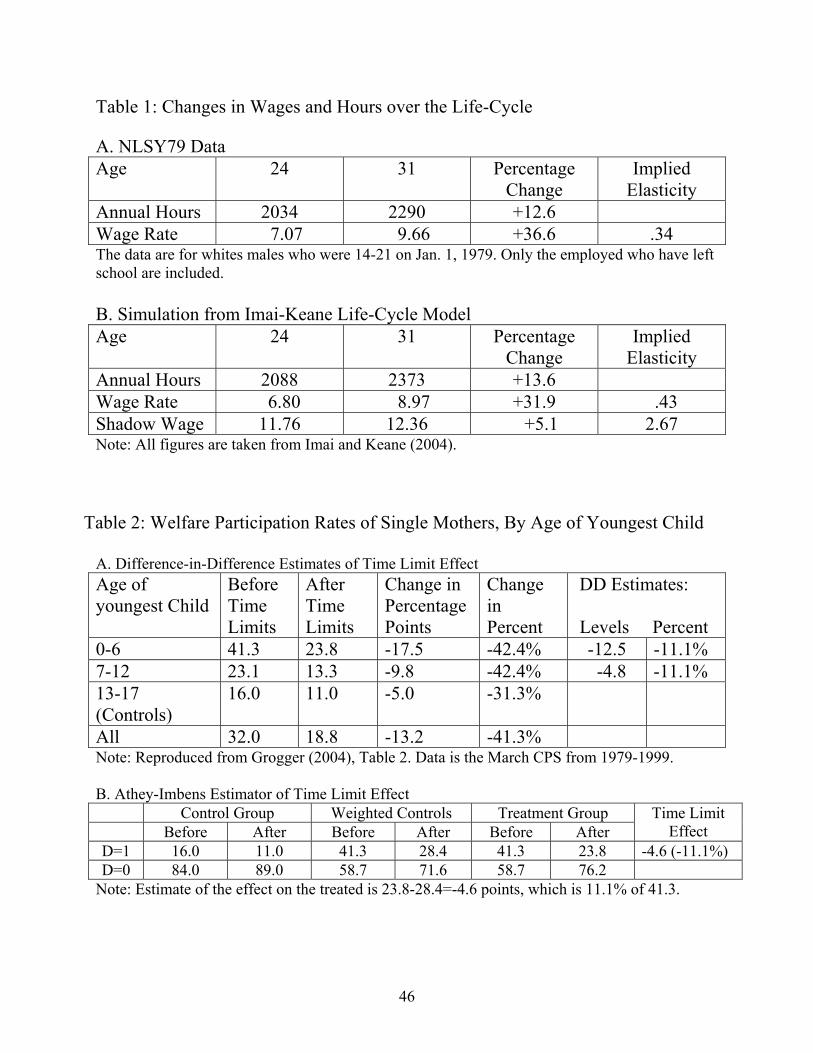
Table 1: Changes in Wages and Hours over the Life-Cycle A. NLSY79 Data Age 24 31 Percentage

Change Implied

Elasticity Annual Hours 2034 2290 +12.6 Wage Rate 7.07 9.66 +36.6 .34 The data are for whites males who were 14-21 on Jan. 1, 1979. Only the employed who have left school are included. B. Simulation from Imai-Keane Life-Cycle Model Age 24 31 Percentage

Change Implied

Elasticity Annual Hours 2088 2373 +13.6 Wage Rate 6.80 8.97 +31.9 .43 Shadow Wage 11.76 12.36 +5.1 2.67 Note: All figures are taken from Imai and Keane (2004).

Table 2: Welfare Participation Rates of Single Mothers, By Age of Youngest Child

A. Difference-in-Difference Estimates of Time Limit Effect Age of youngest Child

Before Time Limits

After Time Limits

Change in Percentage Points

Change in Percent

DD Estimates: Levels Percent

0-6 41.3 23.8 -17.5 -42.4% -12.5 -11.1% 7-12 23.1 13.3 -9.8 -42.4% -4.8 -11.1% 13-17 (Controls)

16.0 11.0 -5.0 -31.3%

All 32.0 18.8 -13.2 -41.3% Note: Reproduced from Grogger (2004), Table 2. Data is the March CPS from 1979-1999. B. Athey-Imbens Estimator of Time Limit Effect

Control Group Weighted Controls Treatment Group Before After Before After Before After

Time Limit Effect

D=1 16.0 11.0 41.3 28.4 41.3 23.8 -4.6 (-11.1%) D=0 84.0 89.0 58.7 71.6 58.7 76.2

Note: Estimate of the effect on the treated is 23.8-28.4=-4.6 points, which is 11.1% of 41.3.

46

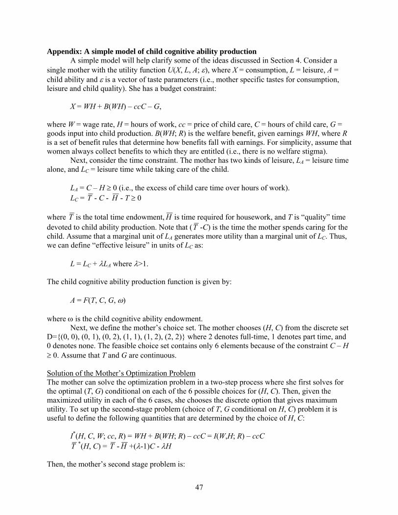
Appendix: A simple model of child cognitive ability production A simple model will help clarify some of the ideas discussed in Section 4. Consider a

single mother with the utility function U(X, L, A; ε), where X = consumption, L = leisure, A = child ability and ε is a vector of taste parameters (i.e., mother specific tastes for consumption, leisure and child quality). She has a budget constraint:

X = WH + B(WH) – ccC – G,

where W = wage rate, H = hours of work, cc = price of child care, C = hours of child care, G = goods input into child production. B(WH; R) is the welfare benefit, given earnings WH, where R is a set of benefit rules that determine how benefits fall with earnings. For simplicity, assume that women always collect benefits to which they are entitled (i.e., there is no welfare stigma). Next, consider the time constraint. The mother has two kinds of leisure, LA = leisure time alone, and LC = leisure time while taking care of the child.

LA = C – H ≥ 0 (i.e., the excess of child care time over hours of work). LC = T - C - H - T ≥ 0

where T is the total time endowment, H is time required for housework, and T is “quality” time devoted to child ability production. Note that (T -C) is the time the mother spends caring for the child. Assume that a marginal unit of LA generates more utility than a marginal unit of LC. Thus, we can define “effective leisure” in units of LC as:

L = LC + λLA where λ>1. The child cognitive ability production function is given by:

A = F(T, C, G, ω) where ω is the child cognitive ability endowment. Next, we define the mother’s choice set. The mother chooses (H, C) from the discrete set D={(0, 0), (0, 1), (0, 2), (1, 1), (1, 2), (2, 2)} where 2 denotes full-time, 1 denotes part time, and 0 denotes none. The feasible choice set contains only 6 elements because of the constraint C – H ≥ 0. Assume that T and G are continuous. Solution of the Mother’s Optimization Problem The mother can solve the optimization problem in a two-step process where she first solves for the optimal (T, G) conditional on each of the 6 possible choices for (H, C). Then, given the maximized utility in each of the 6 cases, she chooses the discrete option that gives maximum utility. To set up the second-stage problem (choice of T, G conditional on H, C) problem it is useful to define the following quantities that are determined by the choice of H, C: I*(H, C, W; cc, R) = WH + B(WH; R) – ccC = I(W,H; R) – ccC

T *(H, C) = T - H +(λ-1)C - λH Then, the mother’s second stage problem is:

47

),,,(

),(

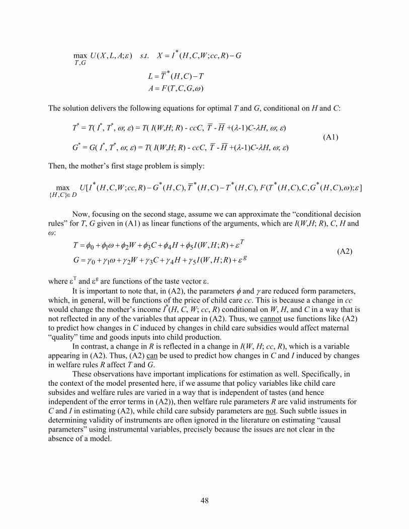
),;,,(..);,,(max

*

*,

ω

ε

GCTFATCHTL

GRccWCHIXtsALXUGT

=−=

−=

The solution delivers the following equations for optimal T and G, conditional on H and C: T* = T( I*, T*, ω; ε) = T( I(W,H; R) - ccC, T - H +(λ-1)C-λH, ω; ε) (A1) G* = G( I*, T*, ω; ε) = T( I(W,H; R) - ccC, T - H +(λ-1)C-λH, ω; ε) Then, the mother’s first stage problem is simply:

]);),,(,),,((),,(),(),,(),;,,([max ******},{

εωCHGCCHTFCHTCHTCHGRccWCHIUDCH

−−∈

Now, focusing on the second stage, assume we can approximate the “conditional decision

rules” for T, G given in (A1) as linear functions of the arguments, which are I(W,H; R), C, H and ω:

(A2) g

T

RHWIHCWG

RHWIHCWT

εγγγγωγγ

εφφφφωφφ

++++++=

++++++=

);,(

);,(

543210

543210

where εT and εg are functions of the taste vector ε.

It is important to note that, in (A2), the parameters φ and γ are reduced form parameters, which, in general, will be functions of the price of child care cc. This is because a change in cc would change the mother’s income I*(H, C, W; cc, R) conditional on W, H, and C in a way that is not reflected in any of the variables that appear in (A2). Thus, we cannot use functions like (A2) to predict how changes in C induced by changes in child care subsidies would affect maternal “quality” time and goods inputs into child production.

In contrast, a change in R is reflected in a change in I(W, H; cc, R), which is a variable appearing in (A2). Thus, (A2) can be used to predict how changes in C and I induced by changes in welfare rules R affect T and G. These observations have important implications for estimation as well. Specifically, in the context of the model presented here, if we assume that policy variables like child care subsides and welfare rules are varied in a way that is independent of tastes (and hence independent of the error terms in (A2)), then welfare rule parameters R are valid instruments for C and I in estimating (A2), while child care subsidy parameters are not. Such subtle issues in determining validity of instruments are often ignored in the literature on estimating “causal parameters” using instrumental variables, precisely because the issues are not clear in the absence of a model.

48