Students guide to laboratory exercise

Students’ guide to

laboratory exercise

”Malware analysis”

March 2016

Laboratory exercise was developed by

Roland Kamarás

CrySyS Laboratory

BME, Laboratory of Cryptography and System Security (CrySyS Lab)

2

Table of Contents

I. Introduction, theoretical summary ....................................................................................................... 4

II. Tools to be used during the exercise..................................................................................................... 5

IDA (Interactive DisAssembler) .................................................................................................................. 5

Introduction to IDA ................................................................................................................................ 5

Database files ........................................................................................................................................ 7

Graphical User Interface ........................................................................................................................ 8

Other views ......................................................................................................................................... 14

IDA View-A ........................................................................................................................................... 15

Hex-View-A .......................................................................................................................................... 16

Exports ................................................................................................................................................. 16

Imports ................................................................................................................................................ 17

Names window .................................................................................................................................... 17

Functions window ............................................................................................................................... 19

Strings window .................................................................................................................................... 20

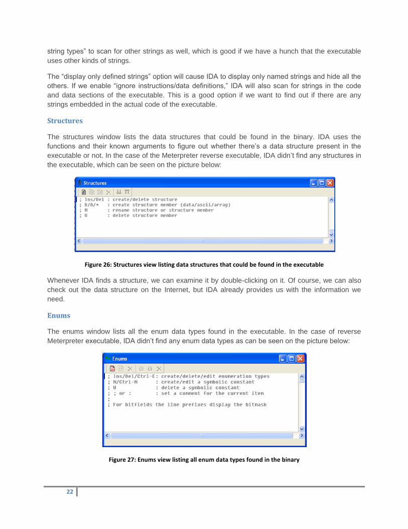
Structures ............................................................................................................................................ 22

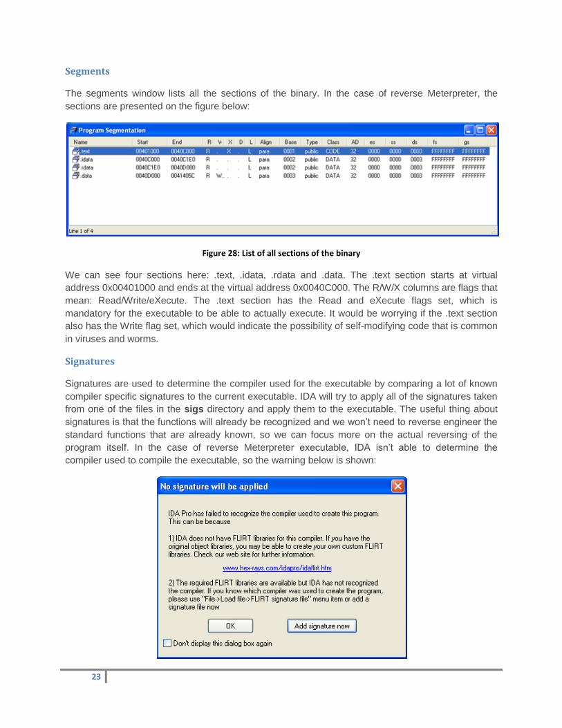
Enums .................................................................................................................................................. 22

Segments ............................................................................................................................................. 23

Signatures ............................................................................................................................................ 23

OllyDbg .................................................................................................................................................... 24

Introduction ......................................................................................................................................... 24

Starting the Debugger ......................................................................................................................... 24

Opening and attaching to the debugging target application .............................................................. 25

The OllyDbg CPU view ......................................................................................................................... 26

Step in, Step over ................................................................................................................................ 27

Exposing history................................................................................................................................... 28

Animation ............................................................................................................................................ 28

Setting breakpoints ............................................................................................................................. 28

Running the code................................................................................................................................. 29

PeID ......................................................................................................................................................... 29

PE Explorer .............................................................................................................................................. 30

3

Unpacking malicious software ............................................................................................................ 32

Rundll32 ................................................................................................................................................... 32

Wireshark ................................................................................................................................................ 33

cURL ......................................................................................................................................................... 33

Web Developer Toolbar .......................................................................................................................... 33

Yara .......................................................................................................................................................... 33

Other applications ................................................................................................................................... 34

HxD ...................................................................................................................................................... 34

Cygwin ................................................................................................................................................. 34

III. Appendix .......................................................................................................................................... 35

Rundll32 ................................................................................................................................................... 35

cURL ......................................................................................................................................................... 35

IV. References ....................................................................................................................................... 36

V. Exercises .............................................................................................................................................. 38

Story ........................................................................................................................................................ 38

Exercises .................................................................................................................................................. 38

VI. Further information ......................................................................................................................... 42

Report ...................................................................................................................................................... 42

4

I. Introduction, theoretical summary

Purpose of the lab exercise is to provide insight into the topic of malware analysis through the

analysis of a fictive malware sample. Students will get this fictive sample at the start of the exercise.

Exercises (see at the end of this guide) are built to perform a realistic and practical malware analysis

workflow (embedded in a story).

Analysis of the fictive malware will be performed with the help of some tools. The list of these tools

and a short description can be read in the following section. After that, we present an introductory

description about these tools such as Interactive DisAssembler and OllyDbg debugger.

Theoretical summary related to this exercise can be found in Memory corruption and Malware

analysis slides (lecture + practice) of Computer Security course:

http://www.hit.bme.hu/~buttyan/courses/BMEVIHIMA06/

The password that is required to download the slides: “ts72ha74w64hd72jq91jaq82j”.

To perform the exercises the Avatao platform will be used, where students will be invited before the

start of the lab exercise.

5

II. Tools to be used during the exercise

During the exercise the following applications will be used:

IDA Pro: A very popular disassembler application.

OllyDbg: Debugger application which can be used to dynamically analyze Windows binaries.

PeID: Packer detection based on signatures (using signature databases).

PE Explorer: Information gathering tool about PE binaries.

Rundll32: Invoking export functions of a DLL.

Wireshark: Network protocol analyzer tool for Unix and Windows.

cURL: Tool for client-side URL transfers (for transferring data with URL syntax).

Mozilla Firefox and Web Developer Toolbar: Browser and browser extension that adds

editing and debugging tools for web developers.

Yara: A pattern matching tool aimed at helping malware researchers to identify and classify

malware samples.

HxD: A freeware hex editor application.

Cygwin: Linux-like environment for Windows making it possible to port software running on

POSIX systems to Windows.

Free version of Visual Studio: Community Free Edition of Visual Studio 2013.

IDA (Interactive DisAssembler)

Introduction to IDA

IDA Pro is probably the best disassembler in the business. Although it costs a lot, there’s still a free

version available. We can download IDA Pro 6.2 limited edition, which is free but only supports

disassembly of x86 and ARM programs. Otherwise, it supports a myriad of other platforms, which we

won’t need here.

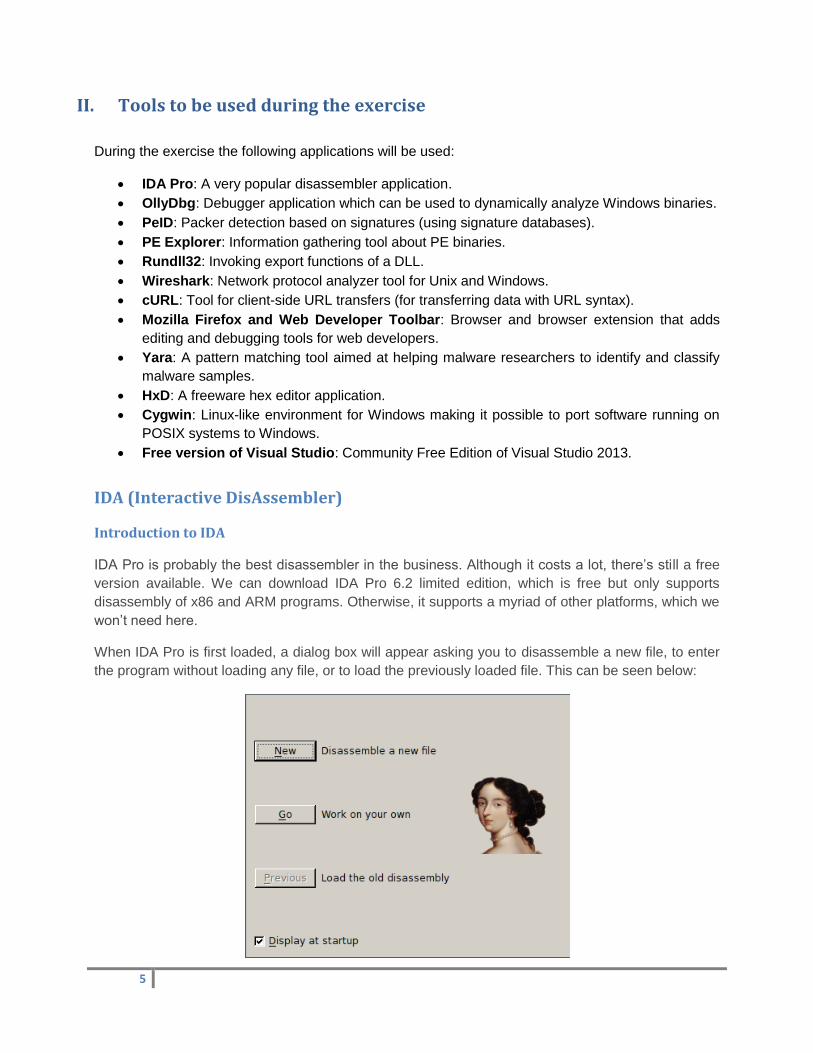
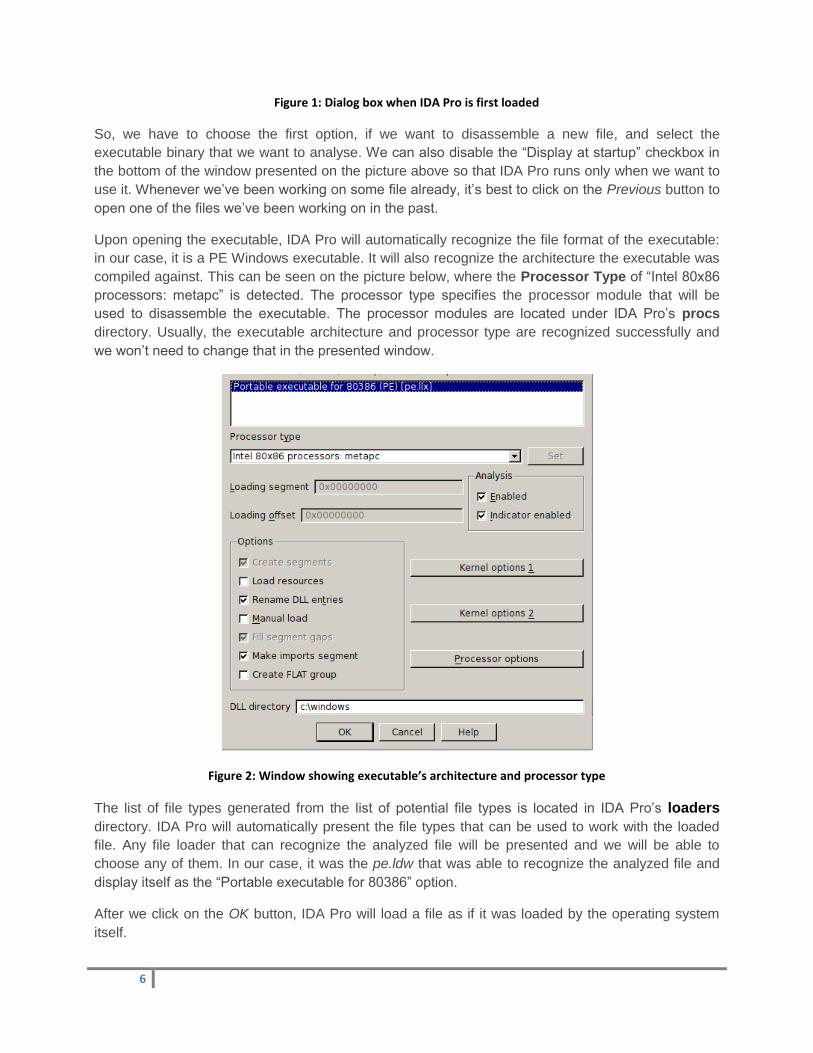
When IDA Pro is first loaded, a dialog box will appear asking you to disassemble a new file, to enter

the program without loading any file, or to load the previously loaded file. This can be seen below:

6

Figure 1: Dialog box when IDA Pro is first loaded

So, we have to choose the first option, if we want to disassemble a new file, and select the

executable binary that we want to analyse. We can also disable the “Display at startup” checkbox in

the bottom of the window presented on the picture above so that IDA Pro runs only when we want to

use it. Whenever we’ve been working on some file already, it’s best to click on the Previous button to

open one of the files we’ve been working on in the past.

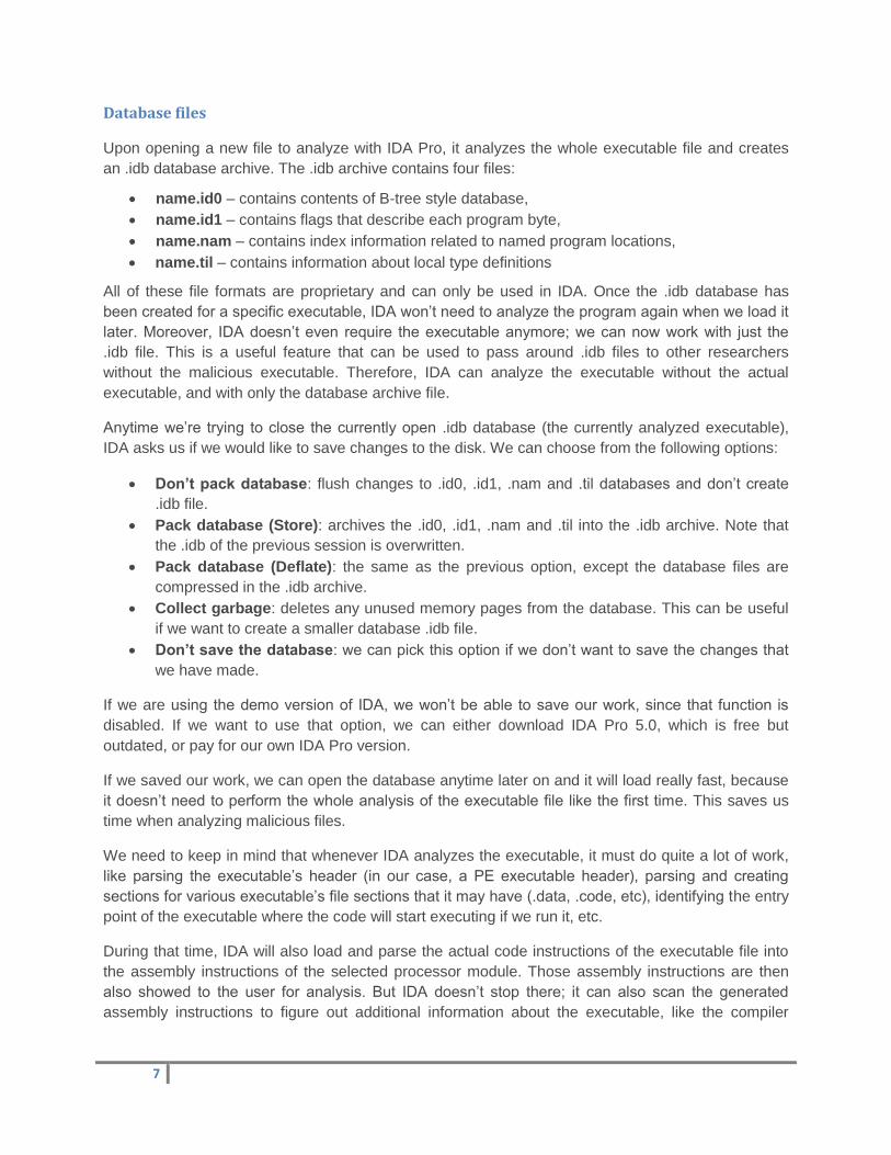
Upon opening the executable, IDA Pro will automatically recognize the file format of the executable:

in our case, it is a PE Windows executable. It will also recognize the architecture the executable was

compiled against. This can be seen on the picture below, where the Processor Type of “Intel 80x86

processors: metapc” is detected. The processor type specifies the processor module that will be

used to disassemble the executable. The processor modules are located under IDA Pro’s procs

directory. Usually, the executable architecture and processor type are recognized successfully and

we won’t need to change that in the presented window.

Figure 2: Window showing executable’s architecture and processor type

The list of file types generated from the list of potential file types is located in IDA Pro’s loaders

directory. IDA Pro will automatically present the file types that can be used to work with the loaded

file. Any file loader that can recognize the analyzed file will be presented and we will be able to

choose any of them. In our case, it was the pe.ldw that was able to recognize the analyzed file and

display itself as the “Portable executable for 80386” option.

After we click on the OK button, IDA Pro will load a file as if it was loaded by the operating system

itself.

7

Database files

Upon opening a new file to analyze with IDA Pro, it analyzes the whole executable file and creates

an .idb database archive. The .idb archive contains four files:

name.id0 – contains contents of B-tree style database,

name.id1 – contains flags that describe each program byte,

name.nam – contains index information related to named program locations,

name.til – contains information about local type definitions

All of these file formats are proprietary and can only be used in IDA. Once the .idb database has

been created for a specific executable, IDA won’t need to analyze the program again when we load it

later. Moreover, IDA doesn’t even require the executable anymore; we can now work with just the

.idb file. This is a useful feature that can be used to pass around .idb files to other researchers

without the malicious executable. Therefore, IDA can analyze the executable without the actual

executable, and with only the database archive file.

Anytime we’re trying to close the currently open .idb database (the currently analyzed executable),

IDA asks us if we would like to save changes to the disk. We can choose from the following options:

Don’t pack database: flush changes to .id0, .id1, .nam and .til databases and don’t create

.idb file.

Pack database (Store): archives the .id0, .id1, .nam and .til into the .idb archive. Note that

the .idb of the previous session is overwritten.

Pack database (Deflate): the same as the previous option, except the database files are

compressed in the .idb archive.

Collect garbage: deletes any unused memory pages from the database. This can be useful

if we want to create a smaller database .idb file.

Don’t save the database: we can pick this option if we don’t want to save the changes that

we have made.

If we are using the demo version of IDA, we won’t be able to save our work, since that function is

disabled. If we want to use that option, we can either download IDA Pro 5.0, which is free but

outdated, or pay for our own IDA Pro version.

If we saved our work, we can open the database anytime later on and it will load really fast, because

it doesn’t need to perform the whole analysis of the executable file like the first time. This saves us

time when analyzing malicious files.

We need to keep in mind that whenever IDA analyzes the executable, it must do quite a lot of work,

like parsing the executable’s header (in our case, a PE executable header), parsing and creating

sections for various executable’s file sections that it may have (.data, .code, etc), identifying the entry

point of the executable where the code will start executing if we run it, etc.

During that time, IDA will also load and parse the actual code instructions of the executable file into

the assembly instructions of the selected processor module. Those assembly instructions are then

also showed to the user for analysis. But IDA doesn’t stop there; it can also scan the generated

assembly instructions to figure out additional information about the executable, like the compiler

8

which was used to compile the executable, the function’s arguments, the function’s local variables,

etc.

All in all, IDA can be very helpful in analyzing an executable by providing various information that we

normally would have had to figure out ourselves.

Graphical User Interface

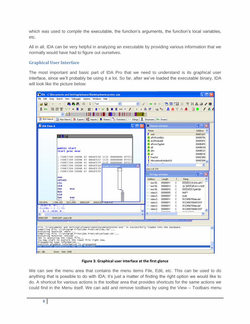
The most important and basic part of IDA Pro that we need to understand is its graphical user

interface, since we’ll probably be using it a lot. So far, after we’ve loaded the executable binary, IDA

will look like the picture below:

Figure 3: Graphical user interface at the first glance

We can see the menu area that contains the menu items File, Edit, etc. This can be used to do

anything that is possible to do with IDA; it’s just a matter of finding the right option we would like to

do. A shortcut for various actions is the toolbar area that provides shortcuts for the same actions we

could find in the Menu itself. We can add and remove toolbars by using the View – Toolbars menu

9

option. The next thing is an overview navigator, which is also presented on the picture below for

clarity:

Figure 4: Overview navigator showing different memory regions

It represents the whole memory space used by the analyzed application. If we right-click on it, we

can zoom in and out to represent smaller chunks of memory. We can also see that different colors

are used for different parts of the memory; this depends on the type of data or code being loaded into

that area. At the very beginning of the navigator, we can see a very small yellow arrow that points to

the location where we’re currently at in the disassembly window.

On the picture below, we’re presenting the different views on the gathered data. The data was

gathered on the initial analysis of the executable and now we’re merely asking IDA to return a

specific type of data in its own data view.

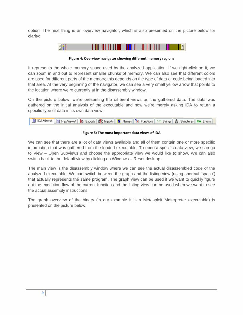
Figure 5: The most important data views of IDA

We can see that there are a lot of data views available and all of them contain one or more specific

information that was gathered from the loaded executable. To open a specific data view, we can go

to View – Open Subviews and choose the appropriate view we would like to show. We can also

switch back to the default view by clicking on Windows – Reset desktop.

The main view is the disassembly window where we can see the actual disassembled code of the

analyzed executable. We can switch between the graph and the listing view (using shortcut ‘space’)

that actually represents the same program. The graph view can be used if we want to quickly figure

out the execution flow of the current function and the listing view can be used when we want to see

the actual assembly instructions.

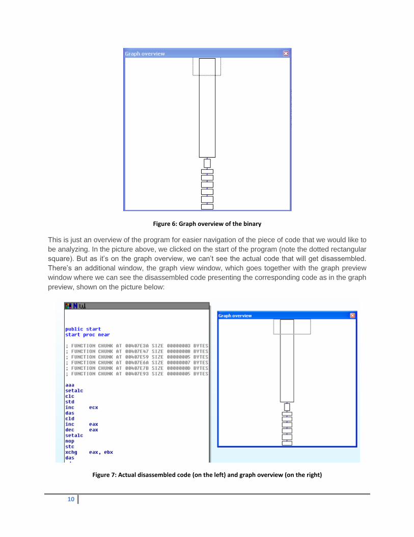
The graph overview of the binary (in our example it is a Metasploit Meterpreter executable) is

presented on the picture below:

10

Figure 6: Graph overview of the binary

This is just an overview of the program for easier navigation of the piece of code that we would like to

be analyzing. In the picture above, we clicked on the start of the program (note the dotted rectangular

square). But as it’s on the graph overview, we can’t see the actual code that will get disassembled.

There’s an additional window, the graph view window, which goes together with the graph preview

window where we can see the disassembled code presenting the corresponding code as in the graph

preview, shown on the picture below:

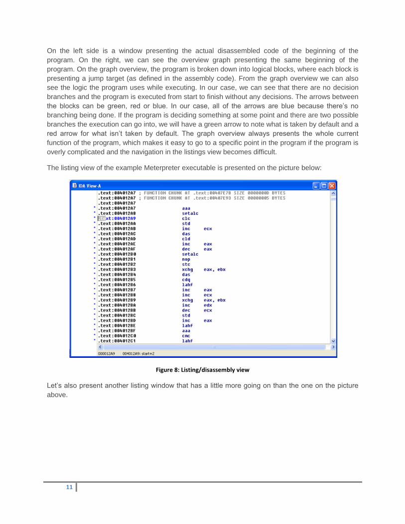
Figure 7: Actual disassembled code (on the left) and graph overview (on the right)

11

On the left side is a window presenting the actual disassembled code of the beginning of the

program. On the right, we can see the overview graph presenting the same beginning of the

program. On the graph overview, the program is broken down into logical blocks, where each block is

presenting a jump target (as defined in the assembly code). From the graph overview we can also

see the logic the program uses while executing. In our case, we can see that there are no decision

branches and the program is executed from start to finish without any decisions. The arrows between

the blocks can be green, red or blue. In our case, all of the arrows are blue because there’s no

branching being done. If the program is deciding something at some point and there are two possible

branches the execution can go into, we will have a green arrow to note what is taken by default and a

red arrow for what isn’t taken by default. The graph overview always presents the whole current

function of the program, which makes it easy to go to a specific point in the program if the program is

overly complicated and the navigation in the listings view becomes difficult.

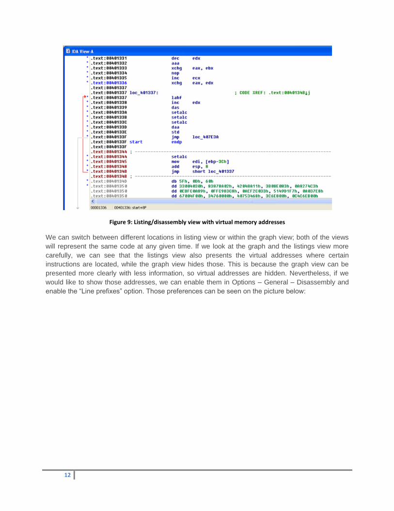
The listing view of the example Meterpreter executable is presented on the picture below:

Figure 8: Listing/disassembly view

Let’s also present another listing window that has a little more going on than the one on the picture

above.

12

Figure 9: Listing/disassembly view with virtual memory addresses

We can switch between different locations in listing view or within the graph view; both of the views

will represent the same code at any given time. If we look at the graph and the listings view more

carefully, we can see that the listings view also presents the virtual addresses where certain

instructions are located, while the graph view hides those. This is because the graph view can be

presented more clearly with less information, so virtual addresses are hidden. Nevertheless, if we

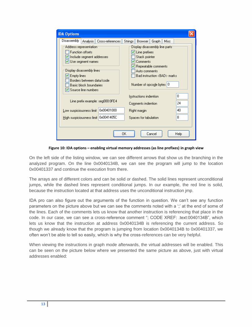
would like to show those addresses, we can enable them in Options – General – Disassembly and

enable the “Line prefixes” option. Those preferences can be seen on the picture below:

13

Figure 10: IDA options – enabling virtual memory addresses (as line prefixes) in graph view

On the left side of the listing window, we can see different arrows that show us the branching in the

analyzed program. On the line 0x0040134B, we can see the program will jump to the location

0x00401337 and continue the execution from there.

The arrays are of different colors and can be solid or dashed. The solid lines represent unconditional

jumps, while the dashed lines represent conditional jumps. In our example, the red line is solid,

because the instruction located at that address uses the unconditional instruction jmp.

IDA pro can also figure out the arguments of the function in question. We can’t see any function

parameters on the picture above but we can see the comments noted with a ‘;’ at the end of some of

the lines. Each of the comments lets us know that another instruction is referencing that place in the

code. In our case, we can see a cross-reference comment “; CODE XREF: .text:0040134B”, which

lets us know that the instruction at address 0x0040134B is referencing the current address. So

though we already know that the program is jumping from location 0x0040134B to 0x00401337, we

often won’t be able to tell so easily, which is why the cross-references can be very helpful.

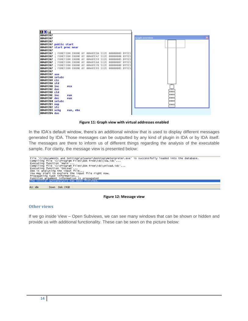
When viewing the instructions in graph mode afterwards, the virtual addresses will be enabled. This

can be seen on the picture below where we presented the same picture as above, just with virtual

addresses enabled:

14

Figure 11: Graph view with virtual addresses enabled

In the IDA’s default window, there’s an additional window that is used to display different messages

generated by IDA. Those messages can be outputted by any kind of plugin in IDA or by IDA itself.

The messages are there to inform us of different things regarding the analysis of the executable

sample. For clarity, the message view is presented below:

Figure 12: Message view

Other views

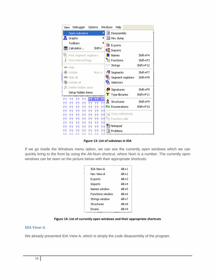
If we go inside View – Open Subviews, we can see many windows that can be shown or hidden and

provide us with additional functionality. These can be seen on the picture below:

15

Figure 13: List of subviews in IDA

If we go inside the Windows menu option, we can see the currently open windows which we can

quickly bring to the front by using the Alt-Num shortcut, where Num is a number. The currently open

windows can be seen on the picture below with their appropriate shortcuts:

Figure 14: List of currently open windows and their appropriate shortcuts

IDA View-A

We already presented IDA View-A, which is simply the code disassembly of the program.

16

Hex-View-A

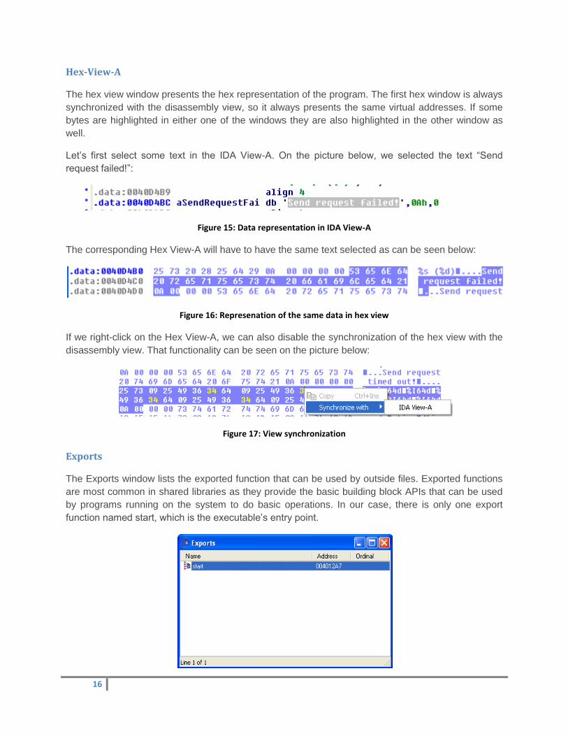
The hex view window presents the hex representation of the program. The first hex window is always

synchronized with the disassembly view, so it always presents the same virtual addresses. If some

bytes are highlighted in either one of the windows they are also highlighted in the other window as

well.

Let’s first select some text in the IDA View-A. On the picture below, we selected the text “Send

request failed!”:

Figure 15: Data representation in IDA View-A

The corresponding Hex View-A will have to have the same text selected as can be seen below:

Figure 16: Represenation of the same data in hex view

If we right-click on the Hex View-A, we can also disable the synchronization of the hex view with the

disassembly view. That functionality can be seen on the picture below:

Figure 17: View synchronization

Exports

The Exports window lists the exported function that can be used by outside files. Exported functions

are most common in shared libraries as they provide the basic building block APIs that can be used

by programs running on the system to do basic operations. In our case, there is only one export

function named start, which is the executable’s entry point.

17

Figure 18: Exports window showing the entry point of the executable

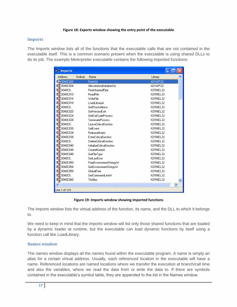
Imports

The Imports window lists all of the functions that the executable calls that are not contained in the

executable itself. This is a common scenario present when the executable is using shared DLLs to

do its job. The example Meterpreter executable contains the following imported functions:

Figure 19: Imports window showing imported functions

The imports window lists the virtual address of the function, its name, and the DLL to which it belongs

to.

We need to keep in mind that the imports window will list only those shared functions that are loaded

by a dynamic loader at runtime, but the executable can load dynamic functions by itself using a

function call like LoadLibrary.

Names window

The names window displays all the names found within the executable program. A name is simply an

alias for a certain virtual address. Usually, each referenced location in the executable will have a

name. Referenced locations are named locations where we transfer the execution at branch/call time

and also the variables, where we read the data from or write the data to. If there are symbols

contained in the executable’s symbol table, they are appended to the list in the Names window.

18

Throughout the disassembled code, we can also notice the names that do not appear in the names

window; those are automatically generated by IDA itself. This happens because the symbol table in

the executable doesn’t contain the relevant symbol, which could be inherited. The automatically

generated names usually have one of the following prefixes followed by their corresponding virtual

address: sub_, loc_, byte_, word_, dword_ and unk_.

We can use names to quickly jump to various locations inside the program executable without having

to remember their corresponding virtual addresses. The names window for the example Meterpreter

executable can be seen on the picture below:

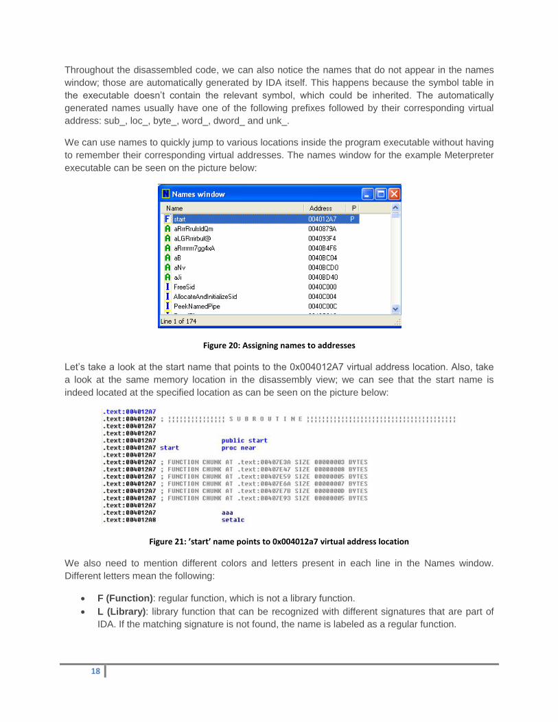
Figure 20: Assigning names to addresses

Let’s take a look at the start name that points to the 0x004012A7 virtual address location. Also, take

a look at the same memory location in the disassembly view; we can see that the start name is

indeed located at the specified location as can be seen on the picture below:

Figure 21: ’start’ name points to 0x004012a7 virtual address location

We also need to mention different colors and letters present in each line in the Names window.

Different letters mean the following:

F (Function): regular function, which is not a library function.

L (Library): library function that can be recognized with different signatures that are part of

IDA. If the matching signature is not found, the name is labeled as a regular function.

19

I (Imported): imported name from the shared library. The code from this function/name is not

present in the executable and is provided at run time, whereas the library function is

embedded into the executable.

C (Code): named code that represent program locations that are not part of any function,

which can happen if the name is a part of the symbol table, but the executable never calls

this function.

D (Data): named data locations that are usually global variables.

A (Ascii): ASCII string data that represents a string terminated with a null byte in the

executable.

In the example Meterpreter executable, we can see that the start name is a regular function, which

means it’s an actual function in the executable. There are also quite a lot of ASCII strings

represented by the letter A. This is normally the case for every executable, since each executable

must contain its share of strings. But the Meterpreter executable also uses imported (I) entries that

correspond to the imported library functions, which are also needed if we want to call functions

outside of the executable (located in shared libraries).

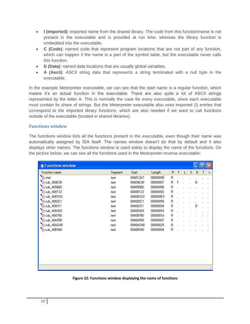
Functions window

The functions window lists all the functions present in the executable, even though their name was

automatically assigned by IDA itself. The names window doesn’t do that by default and it also

displays other names. The functions window is used solely to display the name of the functions. On

the picture below, we can see all the functions used in the Meterpreter reverse executable:

Figure 22: Functions window displaying the name of functions

20

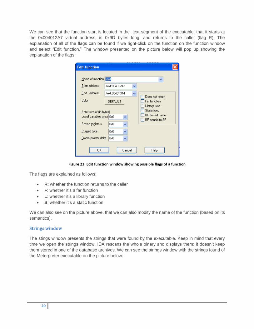
We can see that the function start is located in the .text segment of the executable, that it starts at

the 0x004012A7 virtual address, is 0x9D bytes long, and returns to the caller (flag R). The

explanation of all of the flags can be found if we right-click on the function on the function window

and select “Edit function.” The window presented on the picture below will pop up showing the

explanation of the flags:

Figure 23: Edit function window showing possible flags of a function

The flags are explained as follows:

R: whether the function returns to the caller

F: whether it’s a far function

L: whether it’s a library function

S: whether it’s a static function

We can also see on the picture above, that we can also modify the name of the function (based on its

semantics).

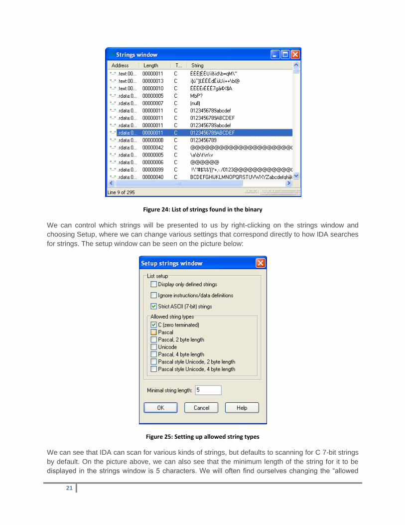
Strings window

The stings window presents the strings that were found by the executable. Keep in mind that every

time we open the strings window, IDA rescans the whole binary and displays them; it doesn’t keep

them stored in one of the database archives. We can see the strings window with the strings found of

the Meterpreter executable on the picture below:

21

Figure 24: List of strings found in the binary

We can control which strings will be presented to us by right-clicking on the strings window and

choosing Setup, where we can change various settings that correspond directly to how IDA searches

for strings. The setup window can be seen on the picture below:

Figure 25: Setting up allowed string types

We can see that IDA can scan for various kinds of strings, but defaults to scanning for C 7-bit strings

by default. On the picture above, we can also see that the minimum length of the string for it to be

displayed in the strings window is 5 characters. We will often find ourselves changing the “allowed

22

string types” to scan for other strings as well, which is good if we have a hunch that the executable

uses other kinds of strings.

The “display only defined strings” option will cause IDA to display only named strings and hide all the

others. If we enable “ignore instructions/data definitions,” IDA will also scan for strings in the code

and data sections of the executable. This is a good option if we want to find out if there are any

strings embedded in the actual code of the executable.

Structures

The structures window lists the data structures that could be found in the binary. IDA uses the

functions and their known arguments to figure out whether there’s a data structure present in the

executable or not. In the case of the Meterpreter reverse executable, IDA didn’t find any structures in

the executable, which can be seen on the picture below:

Figure 26: Structures view listing data structures that could be found in the executable

Whenever IDA finds a structure, we can examine it by double-clicking on it. Of course, we can also

check out the data structure on the Internet, but IDA already provides us with the information we

need.

Enums

The enums window lists all the enum data types found in the executable. In the case of reverse

Meterpreter executable, IDA didn’t find any enum data types as can be seen on the picture below:

Figure 27: Enums view listing all enum data types found in the binary

23

Segments

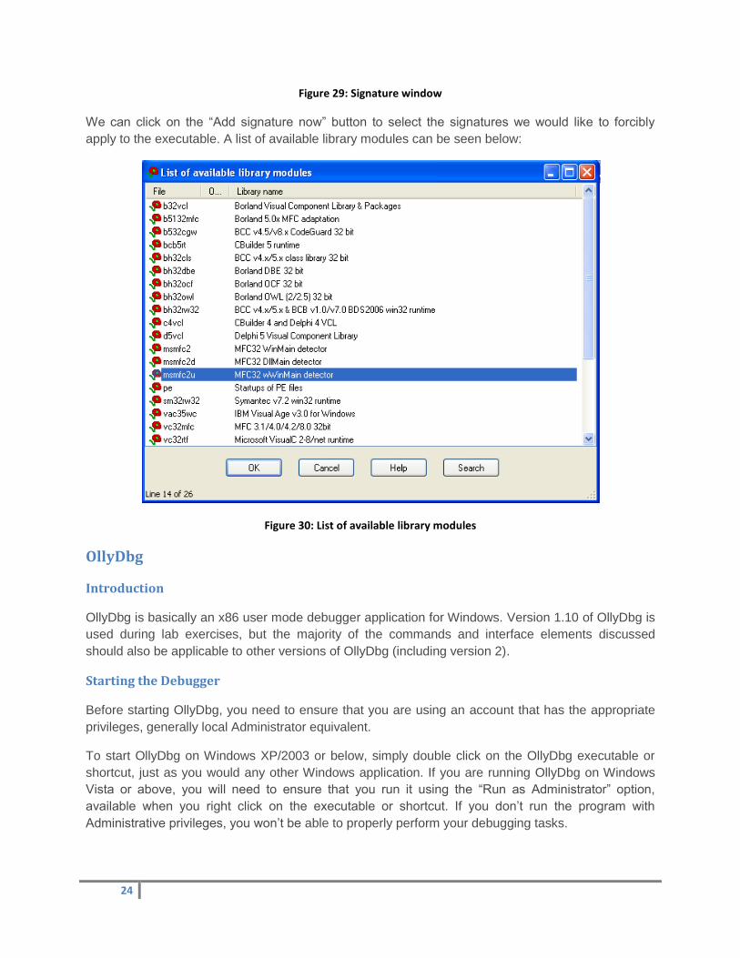
The segments window lists all the sections of the binary. In the case of reverse Meterpreter, the

sections are presented on the figure below:

Figure 28: List of all sections of the binary

We can see four sections here: .text, .idata, .rdata and .data. The .text section starts at virtual

address 0x00401000 and ends at the virtual address 0x0040C000. The R/W/X columns are flags that

mean: Read/Write/eXecute. The .text section has the Read and eXecute flags set, which is

mandatory for the executable to be able to actually execute. It would be worrying if the .text section

also has the Write flag set, which would indicate the possibility of self-modifying code that is common

in viruses and worms.

Signatures

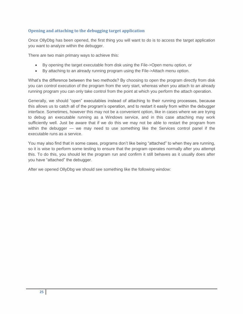
Signatures are used to determine the compiler used for the executable by comparing a lot of known

compiler specific signatures to the current executable. IDA will try to apply all of the signatures taken

from one of the files in the sigs directory and apply them to the executable. The useful thing about

signatures is that the functions will already be recognized and we won’t need to reverse engineer the

standard functions that are already known, so we can focus more on the actual reversing of the

program itself. In the case of reverse Meterpreter executable, IDA isn’t able to determine the

compiler used to compile the executable, so the warning below is shown:

24

Figure 29: Signature window

We can click on the “Add signature now” button to select the signatures we would like to forcibly

apply to the executable. A list of available library modules can be seen below:

Figure 30: List of available library modules

OllyDbg

Introduction

OllyDbg is basically an x86 user mode debugger application for Windows. Version 1.10 of OllyDbg is

used during lab exercises, but the majority of the commands and interface elements discussed

should also be applicable to other versions of OllyDbg (including version 2).

Starting the Debugger

Before starting OllyDbg, you need to ensure that you are using an account that has the appropriate

privileges, generally local Administrator equivalent.

To start OllyDbg on Windows XP/2003 or below, simply double click on the OllyDbg executable or

shortcut, just as you would any other Windows application. If you are running OllyDbg on Windows

Vista or above, you will need to ensure that you run it using the “Run as Administrator” option,

available when you right click on the executable or shortcut. If you don’t run the program with

Administrative privileges, you won’t be able to properly perform your debugging tasks.

25

Opening and attaching to the debugging target application

Once OllyDbg has been opened, the first thing you will want to do is to access the target application

you want to analyze within the debugger.

There are two main primary ways to achieve this:

By opening the target executable from disk using the File->Open menu option, or

By attaching to an already running program using the File->Attach menu option.

What’s the difference between the two methods? By choosing to open the program directly from disk

you can control execution of the program from the very start, whereas when you attach to an already

running program you can only take control from the point at which you perform the attach operation.

Generally, we should “open” executables instead of attaching to their running processes, because

this allows us to catch all of the program’s operation, and to restart it easily from within the debugger

interface. Sometimes, however this may not be a convenient option, like in cases where we are trying

to debug an executable running as a Windows service, and in this case attaching may work

sufficiently well. Just be aware that if we do this we may not be able to restart the program from

within the debugger — we may need to use something like the Services control panel if the

executable runs as a service.

You may also find that in some cases, programs don’t like being “attached” to when they are running,

so it is wise to perform some testing to ensure that the program operates normally after you attempt

this. To do this, you should let the program run and confirm it still behaves as it usually does after

you have “attached” the debugger.

After we opened OllyDbg we should see something like the following window:

26

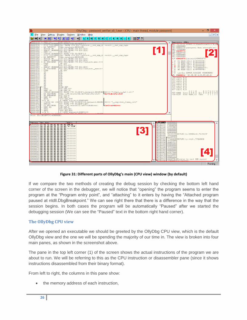
Figure 31: Different parts of OllyDbg’s main (CPU view) window (by default)

If we compare the two methods of creating the debug session by checking the bottom left hand

corner of the screen in the debugger, we will notice that “opening” the program seems to enter the

program at the “Program entry point”, and “attaching” to it enters by having the “Attached program

paused at ntdll.DbgBreakpoint.” We can see right there that there is a difference in the way that the

session begins. In both cases the program will be automatically “Paused” after we started the

debugging session (We can see the “Paused” text in the bottom right hand corner).

The OllyDbg CPU view

After we opened an executable we should be greeted by the OllyDbg CPU view, which is the default

OllyDbg view and the one we will be spending the majority of our time in. The view is broken into four

main panes, as shown in the screenshot above.

The pane in the top left corner (1) of the screen shows the actual instructions of the program we are

about to run. We will be referring to this as the CPU instruction or disassembler pane (since it shows

instructions disassembled from their binary format).

From left to right, the columns in this pane show:

the memory address of each instruction,

27

the hexadecimal representation of each byte that comprises that instruction (or if you prefer,

the “opcode” of that instruction),

the instruction itself in x86 assembly language, shown (by default) in MASM syntax, and

finally

an information/comment column which shows string values, higher level function names, user

defined comments, etc.

So, this top left hand pane is where the assembly instructions are shown.

The pane in the top right hand corner (2) of the screen shows the value of various registers and flags

in the CPU. We will be referring to this as the register pane. These registers are small storage areas

within the CPU itself, and they are used to facilitate various operations that are performed within the

x86 assembly language.

The pane in the bottom left hand corner (3) shows a section of the program’s memory. We will be

referring to this as the memory dump pane. Within this pane you can view memory in a variety of

different formats, as well as copy and even change the contents of that memory.

The pane in the bottom right hand corner (4) shows the stack. We will be referring to this as the stack

pane. The left hand column in this pane contains memory addresses of stack entries, the second

column contains the values of those stack entries, and the right hand column contains information

such as the purpose of particular entries or additional detail about their contents. Each line within the

pane represents an entry on the stack.

There is also an optional third column in the stack pane that will display an ASCII or Unicode dump of

the stack value — this can be enabled by right clicking on the stack pane and selecting either “Show

ASCII dump” or “Show UNICODE dump.”

You have learned about assembly language and about working mechanism of the x86 CPU

(including understanding the purpose of the stack) in Computer Security course (see Memory

corruption and Malware analysis slides (theory + practice)):

http://www.hit.bme.hu/~buttyan/courses/BMEVIHIMA06/

The following password will be necessary to uncompress the archives (containing the slides):

ts72ha74w64hd72jq91jaq82j

You have also met with assembly language in the previous lab exercise (MEMC lab exercise).

Step in, Step over

After we have loaded our executable into OllyDbg, we can step through the code by using OllyDbg’s

single stepping functionality. The F8 key is a shortcut key for the “Step over” operation, which allows

us to advance forward one instruction, while NOT following any function calls.

If we want to actually follow the debugger into the code specified by a CALL statement, we can use

the “Step into” command, which uses F7 as its shortcut key.

28

In the second case, the debugger will follow the call instruction, and will then pause at the beginning

of the called function. Using “Step into” command, we can follow the code referenced by that CALL

instruction.

So the difference between the “Step over” and “Step into” commands is that one steps over CALL

statements (preventing you from having to go through the code there if you don’t want to) and the

other steps into them, allowing the “CALL”ed code to be viewed.

Exposing history

OllyDbg keeps a history of the last 1000 commands that were displayed in the CPU window, so if we

have stepped into a CALL statement, or followed a JMP and we want to remind ourselves of the

previous code location, we can use the plus (+) and minus (–) keys to navigate through the history. If

we try the minus key, the CPU view should then display the last CALL/JMP instruction that we just

executed. We can use the plus key to come back to the current instruction.

Note that this little trick only allows us to view instructions that have actually been displayed and

tracked in the debugger. We can’t let the program run, generate a crash and then use the minus key

to check the instruction just before the crash occurred, nor can you let your program run until it hits a

breakpoint and then step back from there. You can also use the Run trace capabilities of OllyDbg to

achieve this type of functionality.

Animation

If we want to step through our code in a controlled fashion, but don’t like the thought of having to

hammer quickly at the F7 or F8 buttons, we can take advantage of OllyDbg’s animation capabilities.

Press Ctrl-F7 for “Step into” animation and Ctrl-F8 for “Step out” animation. This will step through the

code rather quickly, allowing us to pause once more by hitting the Esc key. We can then use plus (+)

and minus (–) keys to step through the history of our animated session.

Setting breakpoints

Up until now we have maintained more or less manual control over how the program is executed,

with us having to either approve each instruction in advance, or having to let the instructions run in a

semi-automated fashion with us hitting Esc (hopefully at the right time) when we want the program to

stop.

What if we want to stop the program at a particular point in the middle of its execution though? The

step by step method will be too slow (there are a lot of instructions in even the simplest program),

and the animation method will be too imprecise. Well, to allow us to stop at a point of our choosing,

we can use breakpoints, which are essentially markers on particular instructions in the code that tell

the debugger to pause execution when one of those instructions are about to be executed by the

CPU.

If we want to place a breakpoint on an instruction of the program, first we have to highlight the

instruction in the CPU view, and then hit the F2 key, which is used to both set and clear breakpoints.

If we open the View->Breakpoints menu option, or hit Alt-B, we should now also see our breakpoint

listed in the Breakpoints view. You will note that the memory address for that instruction will be

highlighted in red in the top left pane of the CPU View.

29

Running the code

To allow code to run within the debugger, hit the F9 or Run key. The program will now essentially run

normally, until either a breakpoint is hit or an exception occurs. (Strictly speaking, you can manually

pause the program in the debugger too, but that’s often not particularly useful.)

(Generally, when we want to interact with a program in a normal way while we are debugging it, for

example if we want to send data to a program to cause an exception, the F9 Run option is what we

need to use to allow that to happen.)

We can restart the debugged application using Debug->Restart menu option.

We can close the debugging session using the Debug->Close menu option.

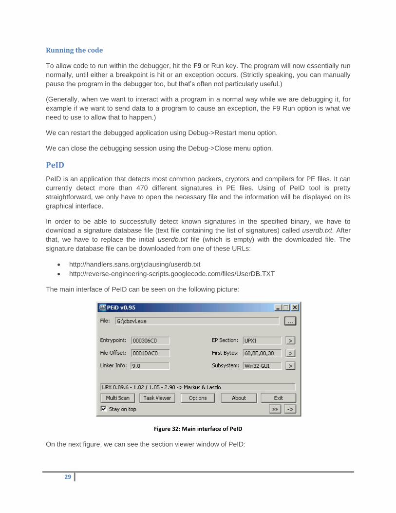
PeID

PeID is an application that detects most common packers, cryptors and compilers for PE files. It can

currently detect more than 470 different signatures in PE files. Using of PeID tool is pretty

straightforward, we only have to open the necessary file and the information will be displayed on its

graphical interface.

In order to be able to successfully detect known signatures in the specified binary, we have to

download a signature database file (text file containing the list of signatures) called userdb.txt. After

that, we have to replace the initial userdb.txt file (which is empty) with the downloaded file. The

signature database file can be downloaded from one of these URLs:

http://handlers.sans.org/jclausing/userdb.txt

http://reverse-engineering-scripts.googlecode.com/files/UserDB.TXT

The main interface of PeID can be seen on the following picture:

Figure 32: Main interface of PeID

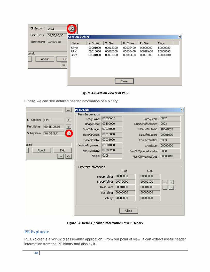
On the next figure, we can see the section viewer window of PeID:

30

Figure 33: Section viewer of PeID

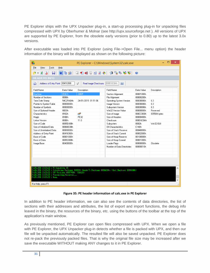
Finally, we can see detailed header information of a binary:

Figure 34: Details (header information) of a PE binary

PE Explorer

PE Explorer is a Win32 disassembler application. From our point of view, it can extract useful header

information from the PE binary and display it.

31

PE Explorer ships with the UPX Unpacker plug-in, a start-up processing plug-in for unpacking files

compressed with UPX by Oberhumer & Molnar (see http://upx.sourceforge.net ). All versions of UPX

are supported by PE Explorer, from the obsolete early versions (prior to 0.80) up to the latest 3.0x

versions.

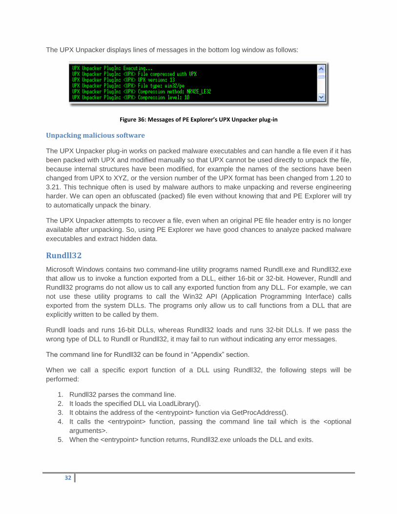
After executable was loaded into PE Explorer (using File->Open File... menu option) the header

information of the binary will be displayed as shown on the following picture:

Figure 35: PE header information of calc.exe in PE Explorer

In addition to PE header information, we can also see the contents of data directories, the list of

sections with their addresses and attributes, the list of export and import functions, the debug info

leaved in the binary, the resources of the binary, etc. using the buttons of the toolbar at the top of the

application’s main window.

As previously mentioned, PE Explorer can open files compressed with UPX. When we open a file

with PE Explorer, the UPX Unpacker plug-in detects whether a file is packed with UPX, and then our

file will be unpacked automatically. The resulted file will also be saved unpacked. PE Explorer does

not re-pack the previously packed files. That is why the original file size may be increased after we

save the executable WITHOUT making ANY changes to it in PE Explorer.

32

The UPX Unpacker displays lines of messages in the bottom log window as follows:

Figure 36: Messages of PE Explorer’s UPX Unpacker plug-in

Unpacking malicious software

The UPX Unpacker plug-in works on packed malware executables and can handle a file even if it has

been packed with UPX and modified manually so that UPX cannot be used directly to unpack the file,

because internal structures have been modified, for example the names of the sections have been

changed from UPX to XYZ, or the version number of the UPX format has been changed from 1.20 to

3.21. This technique often is used by malware authors to make unpacking and reverse engineering

harder. We can open an obfuscated (packed) file even without knowing that and PE Explorer will try

to automatically unpack the binary.

The UPX Unpacker attempts to recover a file, even when an original PE file header entry is no longer

available after unpacking. So, using PE Explorer we have good chances to analyze packed malware

executables and extract hidden data.

Rundll32

Microsoft Windows contains two command-line utility programs named Rundll.exe and Rundll32.exe

that allow us to invoke a function exported from a DLL, either 16-bit or 32-bit. However, Rundll and

Rundll32 programs do not allow us to call any exported function from any DLL. For example, we can

not use these utility programs to call the Win32 API (Application Programming Interface) calls

exported from the system DLLs. The programs only allow us to call functions from a DLL that are

explicitly written to be called by them.

Rundll loads and runs 16-bit DLLs, whereas Rundll32 loads and runs 32-bit DLLs. If we pass the

wrong type of DLL to Rundll or Rundll32, it may fail to run without indicating any error messages.

The command line for Rundll32 can be found in “Appendix” section.

When we call a specific export function of a DLL using Rundll32, the following steps will be

performed:

1. Rundll32 parses the command line.

2. It loads the specified DLL via LoadLibrary().

3. It obtains the address of the <entrypoint> function via GetProcAddress().

4. It calls the <entrypoint> function, passing the command line tail which is the <optional

arguments>.

5. When the <entrypoint> function returns, Rundll32.exe unloads the DLL and exits.

33

Wireshark

Wireshark is an open source packet capturer and network traffic and protocol analyzer application for

Windows and Unix-like operating systems. We assume that students have met with the application

and used it in their previous studies.

cURL

cURL is an open source command line tool and library for transferring data (using it in command

lines or in scripts) with URL syntax, supporting several application layer protocols. cURL supports

SSL certificates, HTTP POST, HTTP PUT, HTTP form based upload, proxies, HTTP/2, cookies,

user+password authentication, file transfer resume, proxy tunneling, etc.

Command line usage of cURL and some important command line options can be found in “Appendix”

section.

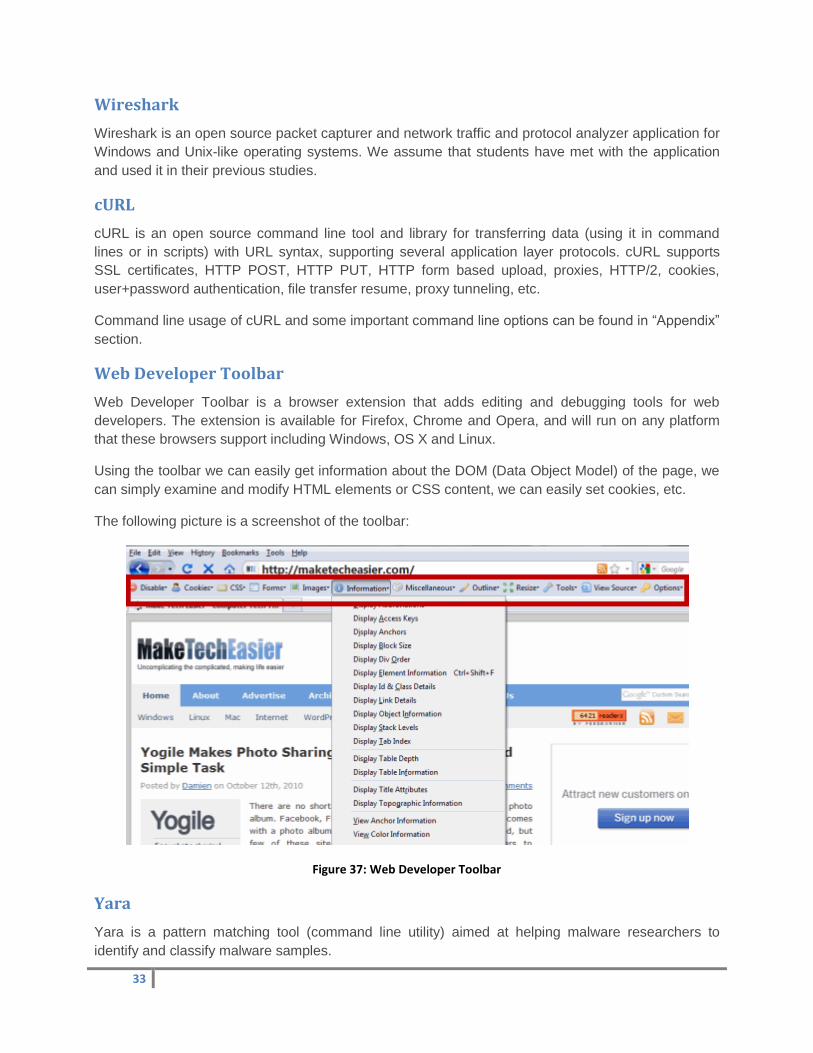
Web Developer Toolbar

Web Developer Toolbar is a browser extension that adds editing and debugging tools for web

developers. The extension is available for Firefox, Chrome and Opera, and will run on any platform

that these browsers support including Windows, OS X and Linux.

Using the toolbar we can easily get information about the DOM (Data Object Model) of the page, we

can simply examine and modify HTML elements or CSS content, we can easily set cookies, etc.

The following picture is a screenshot of the toolbar:

Figure 37: Web Developer Toolbar

Yara

Yara is a pattern matching tool (command line utility) aimed at helping malware researchers to

identify and classify malware samples.

34

Documentation for writing Yara-rules, examples and useful information for using the command-line

utility can be found in the official Yara documentation:

http://yara.readthedocs.org/en/v3.4.0/

Other applications

HxD

Hxd is a freeware hex editor application. It offers features such as searching and replacing,

exporting, checksums/digests, insertion of byte patterns, a file shredder, concatenation or splitting of

files, statistics, etc. Editing in HxD works like in a text editor.

Cygwin

Cygwin is a Linux-like environment for Windows making it possible to port software running on

POSIX systems to Windows. We can use several command-line tools that are available in Unix-like

operating systems like text handler and editor tools (e.g.: grep, sed, head, tail, etc.) or hash

(checksum) generator utilities like md5sum, sha1sum or sha256sum.

35

III. Appendix

Rundll32

The command line for Rundll32 is as follows:

RUNDLL32.EXE <dllname>,<entrypoint> <optional arguments>

An example is as follows:

RUNDLL32.EXE SETUPX.DLL,InstallHinfSection 132 C:\WINDOWS\INF\SHELL.INF

There are 3 issues to consider carefully in the above command line:

o Rundll or Rundll32 search for the given DLL filename in the standard places (see the

documentation for the LoadLibrary() function for details). It is recommended that you

provide a full path to the DLL to ensure that the correct one is found.

o The <dllname> may not contain any spaces or commas or quotation marks. This is a

limitation in the Rundll command line parser.

o In the above command line, the comma (,) between the <dllname> and the

<entrypont> function name is extremely important. If the comma separator is missing,

Rundll or Rundll32 will fail without indicating any errors. In addition, there cannot be

any white spaces in between the <dllname>, the comma, and the <entrypoint>

function.

cURL

The command line for cURL for sending HTTP requests to a server is as follows:

curl <optional arguments> [URL...]

The simplest example is to send a HTTP GET request to a server with verbose output:

curl -v http://example.com

Useful command-line options:

-A/--user-agent <agent string>

Specify the User-Agent string to send to the HTTP server.

-b/--cookie <name=data>

Pass the data to the HTTP server as a cookie.

-d/--data <data>

36

Sends the specified data in a POST request to the HTTP server, in the same way that

a browser does when a user has filled in an HTML form and presses the submit

button.

@filename

This will make curl load data from the given file (including any newlines), URL-encode

that data and pass it on in the POST.

-F/--form <name=content>

This lets curl emulate a filled-in form in which a user has pressed the submit button.

This causes curl to POST data using the Content-Type multipart/form-data. This

enables uploading of binary files etc.

-h/--help

Usage help.

-o/--output <file>

Write output to <file> instead of stdout.

-v/--verbose

Makes the fetching more verbose/talkative. Mostly useful for debugging.

-X/--request <command>

Specifies a custom request method to use when communicating with the HTTP

server. The specified request will be used instead of the method otherwise used

(which defaults to GET). Common additional HTTP requests include POST, PUT and

DELETE.

IV. References

Intel x86 architecture reference

http://www.intel.com/design/pentiumii/manuals/243191.htm

InfoSec Institute: The Basics of IDA Pro

http://resources.infosecinstitute.com/basics-of-ida-pro-2/

Chris Eagle, The IDA Pro Book: The unofficial guide to the world’s most popular

disassembler

Hex-Rays IDA Pro

37

https://www.hex-rays.com/products/ida/

InfoSec Institute: OllyDbg introduction

http://resources.infosecinstitute.com/debugging-fundamentals-for-exploit-development/

http://resources.infosecinstitute.com/in-depth-seh-exploit-writing-tutorial-using-ollydbg/

Official page of OllyDbg

http://www.ollydbg.de/

PeID

https://www.aldeid.com/wiki/PEiD

Official page of PE Explorer

http://www.pe-explorer.com/peexplorer-tour-disassembler.htm

http://www.pe-explorer.com/peexplorer-tour-upx-unpacker.htm

Short description about Rundll32

https://support.microsoft.com/en-us/kb/164787

Official page of Wireshark

https://www.wireshark.org/

Man page of cURL

http://linux.die.net/man/1/curl

Web Developer Toolbar Firefox extension

https://addons.mozilla.org/en-US/firefox/addon/web-developer/

Official page of Yara and official Yara documentation

https://plusvic.github.io/yara/

http://yara.readthedocs.org/en/v3.4.0/

HxD

https://mh-nexus.de/en/hxd/

Cygwin

https://www.cygwin.com/

38

V. Exercises

Story

A company, which name has to be kept in secret, alerted our malware analyst team to inspect a

suspicious binary file that company's security team found in their private network. The suspicious

binary is an x86 Windows DLL (Dynamic-Link Library) file.

The company's incident response team has already examined the sample, but they don't have

enough experience to reverse the sample and fully understand the functionality of the binary. The

incident response team, based on their preliminary analysis, assumes that the DLL is a malicious

binary (a malware) and it has stolen sensitive information from their internal network in the past few

days.

Based on the initial examination, the sample has been loaded by another Windows executable. So,

this outer component loaded the DLL and called its functions. The outer executable is believed to be

the loader of the previously mentioned internal DLL (which performs the main functionality of the

malware) and also a client component of a C&C (Command and Control) server. Now, we think that

attackers can sent commands to the outer module of the malware in the past, and the outer module

proxies these requests to the internal part. The DLL then executed the required function and sent

back some information to the attackers communicating with their server/servers.

Existence of the mentioned outer component is just a hypothesis, because only the malicious DLL

file was found on some workstations of the company's intranet. We also know that at least two

versions of the DLL exist.

Task of our malware analysis team is to examine version A of the binary in depth, determine the

functionality and internal working of the DLL, and notify company's incident response team when new

information is available about the sample. Once again, the binary is gathered from a workstation of

the victim company, so it is important to keep in mind that possible components of the sample may

contain sensitive information about the company. Treat the sample and information confidentially,

company's privacy is very important.

Another task is to create detection for the malware sample in a form of Yara-rules and finally, the

collected information should be summarized in an analysis report.

Exercises

0) Before the analysis of version A of the sample (DLL), we have some information about

version B which seems to be very similar to A. Try to find new information about the sample.

We know that a coding routine was also used by the attackers in the sample to hide contents

of certain files that were generated by the malware. Find information on the decryption

routine, then implement a decoding script or program skeleton (in arbitrary programming

language) that promise to be useful during the lab exercise.

The following information is known about the second (B) version of the sample:

39

We know the MD5 fingerprint of the DLL which is the following:

d2efc5885c4e0f991ddd6d7efa740605

Find the flag as the solution of the exercise and submit the flag in the Avatao platform.

1) Check the size, timestamp, MD5 and SHA256 fingerprints of the binary and note the

information. Also check the sample in virus databases (e.g.: VirusTotal).

Check if the malware sample is packed and if yes, unpack the binary into a new file.

Examine header information of the Windows binary and note some essential information in

your report document.

Give the solution of the exercise and submit it in the Avatao platform. Specification of the

solution can be found on Avatao platform.

2) Examine the binary using static analysis methods. Examine the following parts of the binary:

strings,

import functions,

export functions,

sections/segments,

and resources if they exist.

What findings, conclusions can be drawn from the available information?

Document any information, screenshots, comments, etc. in your analysis report which can be

considered to be important in terms of analysis and in understanding the internal working of

the malware (e.g.: some parts of a call graph, cross references, etc.).


Specification of the solution can be found on Avatao platform.

3) Determine with the help of static analysis methods that what kind of activities the malware

sample under inspection may do on the victim computer, what could be the intention of the

attackers with the malware?

a. Determine what kind of functionalities the malware has, and with which command-line

parameters the sample can be called? What are the roles of these parameters?

b. Verify your findings in virtual sandbox environment by calling the appropriate export

function of the DLL with the decoded parameter/parameters.

o Examine that what happens when the appropriate export function of the DLL

is called with each parameter?

Summarize your results in the analysis report.



40

4) Based on the initial information, we know that some functions of another version of the

malware were started from a remote C&C server by the attackers.

Your task is to determine whether current sample has a set of functionality that helps to

establish a communication channel to a remote C&C server. If you find evidence of this in the

code, determine that exactly how communicates the malware with the server (e.g.: using

what protocol, with what parameters, etc.) and what kind of information is exchanged

between the server and the binary?

If you've found evidence of a C&C server in the code, determine whether this command and

control server is working even or the attackers have presumably switched off already.

Document your activities and findings in the analysis report.



5) Meanwhile, we found a newer version of the malware sample under inspection which was

uploaded by someone unknown to a server. The address (IP address and port number) of the

server can be found on Avatao platform.

Download the newest version from the given address and compare the downloaded binary

with the older one.

Make sure that the newest sample contains code indicating communication with a C&C

server. If so, determine what C&C server/servers the binary may connect to?

If there is/there are C&C server/servers, try to connect to them and check whether the

server/servers has/have any interface that the attackers could use? If you manage to find

such an interface, gather all relevant information as soon as possible before the attackers

switch off the server (if such server exists).

In case of existence of a C&C server, do the following:

a. Check that any information is downloadable from the C&C server that the

attackers have not been removed, and which were collected from victim

machine/machines. If so, then download these information.

b. Try to upload some information to the server (without running the sample),

and then verify that the upload was successful!

Record any new findings and information in the analysis report.


6) If you previously found any active C&C server/servers to the sample, check that it is/they are

still operational!

Using reverse-engineering methods examine export function/functions of the sample

implementing essential operation (functionality) of the malware. Analyze the code in

disassembly and in pseudo C languages.

41

From the information available at the beginning of the analysis, we know that another version

of the current sample store the collected information in an encrypted log file. Presumable,

that a similar solution was applied in the current binary. Check the hypothesis, and if it's

correct, reverse the encoder routine!

If you feel that you get results more quickly using dynamic analysis methods, analyze the

operation of the sample in a debugger! Keep in mind that the sample can apply some anti-

debugging techniques.

Details of the encoding mechanism should be recorded in the analysis report.



7) Make sure that the malware generate a new encrypted log file in the analysis environment.

Based on the precisely reversed encoding routine, implement a decoder program/script

application in arbitrary programming/scripting language (which is the most convenient for

you).

Check working of the created decoder program/script in a way that you try to decode the

previously generated log file with the help of your program.

Examine the contents of the decoded file.

Record your results, findings, and the newly gathered information in the analysis report!


Information about obtaining the flag also can be found on the platform.

8) Based on the previously decoded log file and the partially reversed binary, determine that

exactly what information is recorded by the malware from the victim's computer. If you feel it

necessary for accurate understanding of the operation of the malware to reverse further parts

of the binary, then analyze further blocks of code (functions).

Substantiate your statements in the report with screenshots of reversed parts of code (E.g.:

Exactly where is the listed information recorded in the reversed code?)

Give definition to the log file's structure.

In case that you previously downloaded information from a C&C server and they seem to be

encrypted, try to decode them. Examine their contents and make statements in the report

document.


9) Create a simple detection in a form of Yara-rule for the samples. Be sure to write such rule

that matches for both samples, while other binaries are not matching or at least minimizes the

number of false positives.

Write down in your report that what intention is behind the creation of your Yara-rule.

42

Check the matching of the Yara rule for the samples.

Submit (upload) the Yara-rule in Avatao platform (then check it). Details can be found on

Avatao platform.

10) Send the analysis report together with your decoding script (or in case of program, the

executable binary and its source code) and the Yara-rule created in the previous exercise to

your lab instructor.

VI. Further information

Report

The report has to be sent to the instructor in PDF format within one week after the laboratory lesson.

The report should include the followings:

Student(s)’ name and his/their neptun code

Name of laboratory exercise

Date/time of laboratory exercise

Solutions of the exercises

The solutions should be sought to describe a concise but clear answer. Based on the description the

solution must be reproducible (long code can be attached to the PDF, you do not necessarily have to

put into it)!

Documents

Students guide to laboratory exercise