Subnanometer Positioning and Drift Compensation With Tunneling Current

180 IEEE TRANSACTIONS ON CONTROL SYSTEMS TECHNOLOGY, VOL. 22, NO. 1, JANUARY 2014

Subnanometer Positioning and Drift CompensationWith Tunneling Current

Sylvain Blanvillain, Alina Voda, Gildas Besançon, and Gabriel Buche

Abstract— This paper introduces tunneling current as a sen-sor to detect and control the displacements of micro- andnanoelectromechanical systems. Because of its extremely smallmagnitude, the tunneling current cannot be used without anappropriate control strategy. A control methodology involvingtwo feedback loops is proposed to control displacements with anaccuracy of 40 pm while also compensating the sensor drift. Withthis strategy, controlling displacements with an amplitude > 1 nmis possible, extending the predicted capabilities of tunnelingcurrent by the literature. The overall approach is a solution forthe control of macro to nano systems and may be embedded inpositioning applications requiring a very high degree of accuracy.

Index Terms— Drifts, electrostatic actuation, flexible cantilever,nanopositioning, picopositioning, piezoactuation, robust control,tunneling current.

I. INTRODUCTION

STUDYING and acting at a scale down to the micrometerrevolutionized research in various domains. Emerging

applications in turn imposed new needs to observe, mea-sure, and control at smaller scales, down to the nanometer.In particular, precise positioning at the nanoscale raises newchallenges and heavily depends upon sensing techniques.Among the most used sensing techniques in positioning appli-cations are optical and capacitive sensing. Capacitive sensingcan be used in embedded applications but is limited to afew nanometers in resolution [1], [2]. Optical techniques, likeinterferometry or photodiodes, are, however, very efficient tomeasure displacements smaller than the nanometer [3] witha large bandwidth. As these techniques use macrometric ormicrometric probes, they are unadapted to study nanoscaleddevices. If the device is too thin, optical beams are notreflected but diffused through the device, leading to falsifiedmeasurements [4]. Consequently, novel motion sensing tech-niques exploiting phenomena specific to the nanoscale must

Manuscript received February 16, 2011; revised November 15, 2012;accepted January 30, 2013. Manuscript received in final form February18, 2013. Date of publication March 28, 2013; date of current versionDecember 17, 2013. Recommended by Associate Editor G. Guo.

S. Blanvillain and A. Voda are with the University Joseph FourierGrenoble 1, Grenoble 38402, France. They are also with the ControlDepartment of the Grenoble Image Parole Signal and Automatic Labora-tory, Grenoble 38402, France (e-mail: [email protected]; [email protected]).

G. Besançon is with the Grenoble Institut National Polytechnique and Insti-tut Universitaire de France, Grenoble 38402, France, and also with the ControlDepartment of the Grenoble Image Parole Signal and Automatic Laboratory,Grenoble 38402, France (e-mail: [email protected]).

G. Buche is with the Control Department of the Grenoble ImageParole Signal and Automatic Laboratory, Grenoble 38402, France (e-mail:[email protected]).

Color versions of one or more of the figures in this paper are availableonline at http://ieeexplore.ieee.org.

Digital Object Identifier 10.1109/TCST.2013.2248364

be explored. Among phenomena specific to the nanoscale,tunneling current drawn scarce attention as a means to positionan object. This quantum phenomenon consists of a very smallcurrent flowing between two electrodes < 1 nm away fromeach other. This current varies with the gap between the twoelectrodes and can thus be a mean to measure the displacementof one electrode with respect to the other. This phenomenonis used as an acceleration sensor [5], [6] as distinguished fromits more established application for surface imaging [7]. Thecapabilities of tunneling current in a positioning frameworkwas investigated theoretically in [8] and [9], highlighting itshigh-gain, high-bandwidth, and low-noise characteristics. In[10], tunneling current was used to measure the gap variationbetween two tunneling electrodes, but within a very limitedrange of a few Ångströms. The need to position a microsystemwith tunneling current was also highlighted in [11], but withoutclosed-loop control. Indeed, the main limitation when usingthe tunneling current is that it vanishes when the gap betweenthe electrodes becomes > 1 nm. As in other nanopositioningapplications, drifts of the setup were also reported to be amongmajor drawbacks [12]–[14]. Finally, the range of magnitude ofthe tunneling current (of order a nanoampere) challenges itsexperimental measurement and control.

This paper presents a setup that generates a tunnelingcurrent to sense the position of an object. With a specificcontrol strategy, we show that it is possible to use the tunnelingcurrent as a mean to position a device with an amplitude> 1 nm (as previously forecasted with a numerical simulationin [15]), while compensating drifts. To do so, the controlstrategy combines two feedback loops: one feedback loopelectrostatically regulates the tunneling current by positioningthe device at < 1 nm from a drifting tunneling tip, and asecond feedback loop controls the drift of the tunneling tip.

The remainder of this paper continues as follows. Section IIdescribes the nanopositioning platform studied in this paper.This is followed by the characterization of the plateformand the dynamical modeling of its open-loop behavior inSection III. Section IV then presents a robust control strategymade of two controllers to: 1) electrostatically regulate thetunneling current and 2) control the device position. Experi-mental results illustrate the very high positioning accuracy ofthe device in Section V. Section VI concludes this paper.

II. DEVICE DESCRIPTION AND DIFFERENCES WITH

SIMILAR TECHNOLOGIES

The nanopositioning system studied in this paper is devel-oped at the Control System Department of the Gipsa-Lab research center. Fig. 1 presents a simplified sketch of

1063-6536 © 2013 IEEE

BLANVILLAIN et al.: SUBNANOMETER POSITIONING AND DRIFT COMPENSATION WITH TUNNELING CURRENT 181

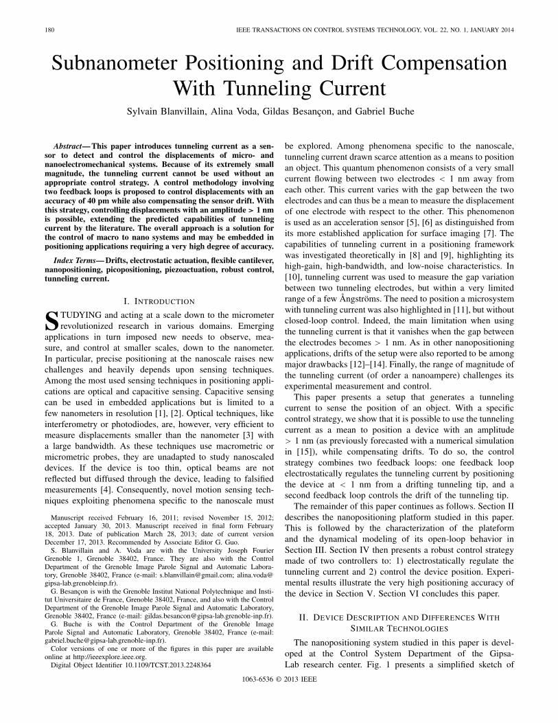
Fig. 1. Simplified sketch of the experimental setup. This picture introducesnotations used in the text. The inputs (Vp and Va ) and the output (y) of theopen-loop system are illustrated with bold arrows.

this system together with the notations used in this paper.The device is situated on an antivibrations table, under ambientconditions (humidity level between 20% and 23%, 1 barpressure).

The device aims at positioning a cantilever in one dimension(the z-direction in Fig. 1) with very high accuracy usingtunneling current. An electrode is set up below and parallelto the cantilever at a distance de between 80 and 30 μm.A potential Va applied between those two elements generatesan electrostatic force F between them. The cantilever movesunder the application of F , providing a displacement z rela-tively to its rest position.

The setup for tunneling current generation and measurementis the following: V0 is a bias voltage between the cantilever andthe tunneling tip. A potential Vp drives a piezoelectric actuator,moving the tunneling tip toward the cantilever. When thetunneling gap g between the tunneling tip and the cantilever is< 1 nm, a tunneling current i appears between the tunnelingtip and the cantilever. A current amplifier, manufactured in ourlaboratory according to [16], finally amplifies the tunnelingcurrent i(t) into a measurable output voltage y(t).

We note that the closeness of the tunneling tip generateselectrostatic and Van der Waals forces on the cantilever. Theseforces tend to attract the cantilever toward the tunneling tipuntil both of them collapse against each other. To preventthis contact, the tunneling tip approaches a rigid part of thecantilever, such that attractive forces only induce a negligibledisplacement of the cantilever. A detailed study about theinfluence of those forces in a positioning framework can befound in [17].

The present device shares some features with scanningtunneling microscopes (STMs), especially a combination oftunneling current and piezoelectric actuator. STMs use apiezoelectric actuator to position a tunneling tip a couple ofÅngströms away from a moving surface. The tunneling currentthen provides a sensing signal to regulate the distance betweenthe tunneling tip and the surface. The tunneling tip then scansthe surface to measure variations of the latter via the controlsignal of the closed-loop [7]. This system is limited by thepositioning of the tunneling tip and by the positioning range(the tunneling current vanishes when the distance between the

tunneling tip and the surface is > 1 nm). Further details aboutSTM instrumentation and feedback can be found for instancein [18] and [19].

In this paper, we demonstrate that tunneling current canbe used to position another object than the tunneling tip(for instance a microcantilever), and, through an appropriatecontrol strategy, with a range of motion > 1 nm. To controla position with a tunneling current based sensor, the simplestapproach would be to use the STM sensing mechanism asdescribed above. This measure might then be fed back tothe electrostatic actuator to control the cantilever position.However, the creep of the piezoelectric actuator generatesa drift that affects the sensing mechanism. This drift biasesthe measured cantilever position, making this measurementmethod not suitable for a real-time positioning purpose. Incontrast with STM technologies, the present device does notaddress the positioning of the tunneling tip relative to a movingsurface, but the positioning of the cantilever relative to thetunneling tip. To do so, we first control the tunneling gap, andthen the position of the tunneling tip. For this purpose, a firstfeedback loop controls the tunneling gap g by continuouslyadjusting the cantilever position relative to the tunneling tip.When the tunneling tip drifts, the cantilever moves with thesame amplitude than the tunneling tip, and the closed-loopcommand of the electrostatic actuator provides a measure ofthe cantilever drift. A second feedback loop then regulates thedrift of the tunneling tip. The device modeling and calibrationare presented in the next section.

III. DEVICE IDENTIFICATION

A. Tunneling Current-Based Sensor

The piezoelectric actuator moving the tunneling tip needsup to 150 V to operate at full displacement range. A voltageamplifier is used for this purpose, amplifying an input voltageVp into a voltage Vva with a gain Gva = 15 V/V over a band-width ωva = 4 kHz. The piezoelectric actuator has a bandwidthfast enough (ωp = 150 kHz) to approximate its dynamicsby its gain Gp = 1.2 nm/V. In closed-loop, the piezoelec-tric actuator generates very small displacements of a fewnanometers, and hence with a negligible hysteresis [20], [21].The dynamics of the tunneling tip position zt can then bemodeled as

Vva(t) = −ωvaVva(t) + GvaωvaVp(t) (1)

zt (t) = −G pVva(t) + dzt (t) (2)

where dzt is a disturbance which gathers the creep of the piezo-electric actuator [20] and the thermal drift of the tunnelingtip. According to several tests in our laboratory, the combinedeffect of both disturbances generates a maximum drift speedof the tunneling tip of 2 nm in 10 s.

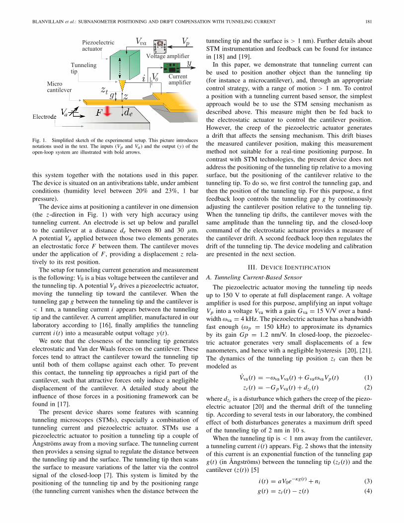
When the tunneling tip is < 1 nm away from the cantilever,a tunneling current i(t) appears. Fig. 2 shows that the intensityof this current is an exponential function of the tunneling gapg(t) (in Ångströms) between the tunneling tip (zt (t)) and thecantilever (z(t)) [5]

i(t) = aV0e−κg(t) + ni (3)

g(t) = zt (t) − z(t) (4)


Fig. 2. Equation (3) (black curve) without noise fits to the experimentalresponse of the tunneling current (grey curve) to validate its exponentialbehavior and to calibrate constants a and κ: a = 0.0011 and κ = 1.65 Å−1.The inset shows noises affecting the tunneling current generated on a mobilesurface.

in which a (dimensionless) and κ (in Å−1) are constants, thelatter depending on work functions of the tip and materialsof the cantilever. V0 = 1.025 V is the bias voltage asshown in Fig. 1. ni gathers the contribution of three noisesillustrated in the inset of Fig. 2. The first noise has a powerspectrum in 1/ f ( f is the frequency) and is dominant atfrequencies under 100 Hz. Such noise is usually recordedin tunneling devices [22]. The second noise is a commonharmonic at 50 Hz. The third noise, named experimental noise,is dominant from 100 to 500 Hz and gathers three peaks whosefrequencies are randomly changing. Ambient vibrations maybe the main origin of this noise. At frequencies > 500 Hz, thefrequency response of the cantilever to the thermal excitationis dominant.

A current amplifier amplifies the tunneling current i(t) witha gain Gca = 109 V/A. Its dynamics is identified as a second-order system with a bandwidth ωca = 13 kHz and a dampingcoefficient γca = 1 such that its output y(t) is

y(t) + 2γcaωca y(t) + ω2ca y(t) = ω2

caGcai(t). (5)

The noise generated by the amplifier is negligible in compar-ison with the tunneling current noise ni .

To establish experimental values of a and κ , and henceto calibrate the sensing mechanism, the piezoelectric actuatormoves the tunneling tip toward a static surface, such asthe clamped extremity of the cantilever. A tunneling currentappears when the tunneling tip reaches 1 nm from the surface,and is measured as a signal function of the tunneling gap (thetunneling gap is deduced from the command of the piezo-electric actuator). The constants a and κ are obtained off-lineby fitting a trendline, with a least square algorithm, on theexperimental response of the tunneling current, as shown byFig. 2. No further calibration is required to setup the tunnelingsensor, as the output of the current amplifier now matches themeasurement range of most acquisition boards (from 0 to 9 V).

B. Electrostatic Actuation

We then generate tunneling current on the cantilever tocalibrate the electrostatic actuator. A potential Va applied

to the electrode actuates the cantilever whose dynamics iscaptured by a second-order system. Defining k the stiffness ofthe cantilever, γc its damping, and ωc its resonance frequency,the acceleration of the cantilever under the application of avoltage Va is [23]

z(t) = ω2c

(−z(t) − 2γcz(t)

ωc− 1

k

ε0 AV 2a (t)

2(de + z(t))2

)(6)

where de is the distance between the cantilever and theelectrode (80 ≤ de ≤ 30 μm), ε0 is the dielectric constantof the air (ε0 ≈ 8.854.10−12 F/m), and A is the common areabetween the cantilever and the electrode (A = 5.104 μm2).

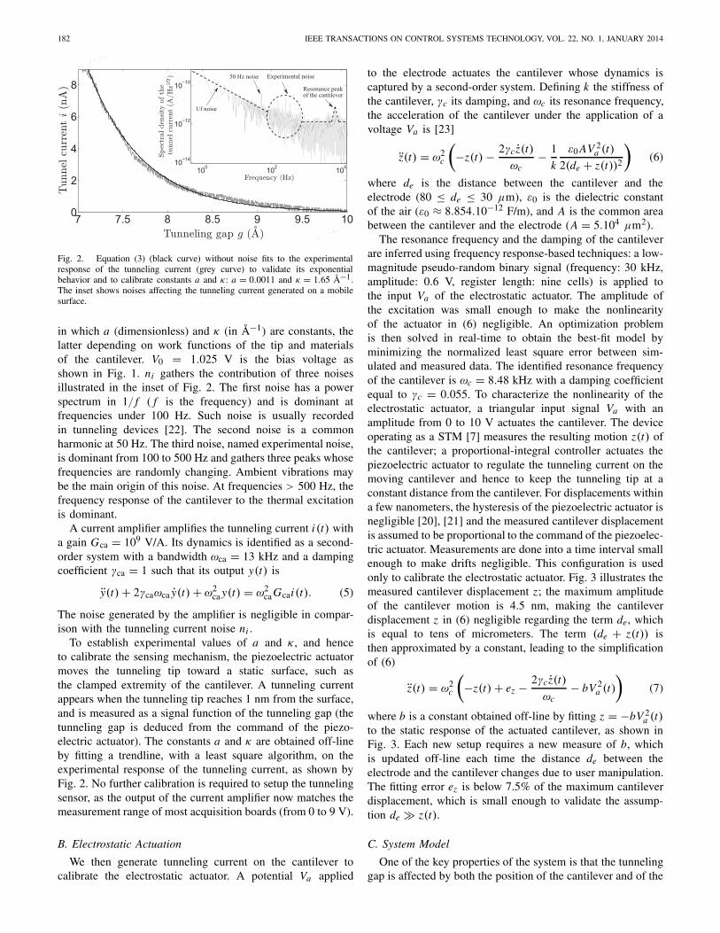
The resonance frequency and the damping of the cantileverare inferred using frequency response-based techniques: a low-magnitude pseudo-random binary signal (frequency: 30 kHz,amplitude: 0.6 V, register length: nine cells) is applied tothe input Va of the electrostatic actuator. The amplitude ofthe excitation was small enough to make the nonlinearityof the actuator in (6) negligible. An optimization problemis then solved in real-time to obtain the best-fit model byminimizing the normalized least square error between sim-ulated and measured data. The identified resonance frequencyof the cantilever is ωc = 8.48 kHz with a damping coefficientequal to γc = 0.055. To characterize the nonlinearity of theelectrostatic actuator, a triangular input signal Va with anamplitude from 0 to 10 V actuates the cantilever. The deviceoperating as a STM [7] measures the resulting motion z(t) ofthe cantilever; a proportional-integral controller actuates thepiezoelectric actuator to regulate the tunneling current on themoving cantilever and hence to keep the tunneling tip at aconstant distance from the cantilever. For displacements withina few nanometers, the hysteresis of the piezoelectric actuator isnegligible [20], [21] and the measured cantilever displacementis assumed to be proportional to the command of the piezoelec-tric actuator. Measurements are done into a time interval smallenough to make drifts negligible. This configuration is usedonly to calibrate the electrostatic actuator. Fig. 3 illustrates themeasured cantilever displacement z; the maximum amplitudeof the cantilever motion is 4.5 nm, making the cantileverdisplacement z in (6) negligible regarding the term de, whichis equal to tens of micrometers. The term (de + z(t)) isthen approximated by a constant, leading to the simplificationof (6)

z(t) = ω2c

(−z(t) + ez − 2γcz(t)

ωc− bV 2

a (t)

)(7)

where b is a constant obtained off-line by fitting z = −bV 2a (t)

to the static response of the actuated cantilever, as shown inFig. 3. Each new setup requires a new measure of b, whichis updated off-line each time the distance de between theelectrode and the cantilever changes due to user manipulation.The fitting error ez is below 7.5% of the maximum cantileverdisplacement, which is small enough to validate the assump-tion de � z(t).

C. System Model

One of the key properties of the system is that the tunnelinggap is affected by both the position of the cantilever and of the


(a)

(b)

Fig. 3. (a) Comparison of the measured displacement. Bold greycurve: electrostatically actuated cantilever. Bold black curve: static modelz = −bV 2

a (t). (b) Fitting error ez is such that |ez | < 0.3 nm.

tunneling tip. This becomes clear when we gather the equa-tions ruling the cantilever and tunneling tip dynamics. The firstsystem input Va actuates the cantilever position z accordingto (7)

z(t) + 2γcωc z(t) + ω2c z(t) = ω2

c

(−bV 2

a (t) + ez

). (8)

From (1) and (2), the second system input Vp actuates thetunneling tip position zt

Vva(t) = −ωvaVva(t) + GvaωvaVp(t) (9)

zt (t) = −G pVva(t) + dzt (t). (10)

The cantilever position z and the tunneling tip position zt thencombine into the tunneling gap

g(t) = zt (t) − z(t). (11)

The tunneling sensor finally translates this gap into the out-put y, with the following dynamics:y(t)+2γcaωca y(t)+ω2

ca y(t)=Gcaω2ca

(aV0e−κg(t) + ni (t)

).

(12)

Fig. 4 sums up this overall system model.

IV. CONTROL DESIGN

A. Overall Control Scheme

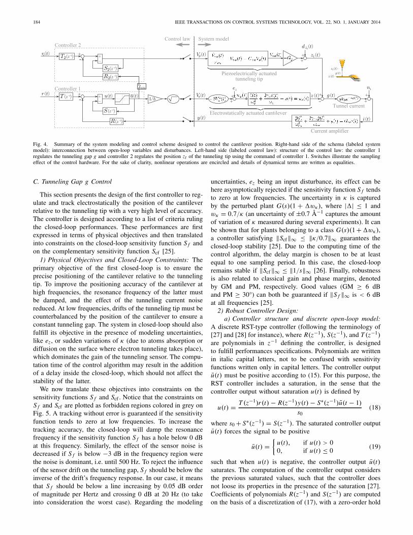
Fig. 4 presents the control scheme adopted to regulatethe cantilever position. We propose a control law made ofone controller for both input of the system. The uncoupleddynamics of the system allow to design both controllers oneafter the other.

The originality of the control scheme is that the outputu(t) of the first controller enters into the second controller,as shown in Fig. 4. To explain it, we shall forecast that thefirst controller aims at regulating the tunneling gap g at aconstant value: it uses variations of the tunneling currentto regulate electrostatically the position of the cantileverrelative to the tunneling tip. The design of this controller isdescribed in Section IV-C. Simultaneously, the tunneling tip

slowly drifts, such that the command of the first controllerslowly evolves to keep the tunneling gap constant. Hence,the evolution of the command corresponds to a variation ofthe position of the tunneling tip. To prevent it, Section IV-Dintroduces a second controller which controls the position ofthe tunneling tip in order to prevent any unwanted variationsof the first controller command. In this way, the addition ofan extra sensor to measure drifts is avoided. Notice that froma practical point of view, this two stage control design couldbe validated step by step. Instead, multivariable couplingswill be analyzed a posteriori, in Section IV-E. A comparisonwith a direct multivariable approach is left for future studies.

B. System Model for the Control Design

To keep the tunneling gap g constant, the control law mustregulate the tunneling current around an equilibrium ieq. Thetunneling current is hence linearized around this equilibrium,which can easily be measured from the output y(t). A first-order Taylor series expansion of (3) around the tunnelingcurrent equilibrium corresponding to i = ieq and ni = 0 yields

g(t) �(

− 1

κlog

(ieq

aV0

))+

(− 1

κieq

)× (i(t) − ieq). (13)

where the term −1/κ log(ieq/aV0

)is equal to the equilibrium

tunneling gap geq corresponding to the equilibrium currentieq. This in turn means that an appropriate dynamics for y(t)around this equilibrium can be given from (12) by

y(t) + 2γcaωca y(t) + ω2ca y(t)

= ω2caGca

(−κieq(g(t) − geq) + ni (t))

= ω2caGcaκieqz(t) + ω2

caGca(−κieqzt (t)

)+ω2

caGca(−κieqgeq + ni (t)

). (14)

On the other hand, to avoid the restriction of the cantilevercontrol around a point of equilibrium, the electrostatic nonlin-earity is tackled by an exact linearization (by the control itself[24]). We choose Va(t) from the controller output denotedby u(t) as

Va(t) =√

u(t)

b(15)

b being the fitting constant defined in (7). For (15) to providea feasible control Va(t), u(t) must be constrained to remainpositive (it will be saturated as explained in Section IV-C.2).From (8), this turns the dynamics for z(t) into

z(t) + 2γcωc z(t) + ω2c z(t) = −ω2

c u(t) + ω2c ez(t). (16)

Finally, from the proposed linearizations, the dynamicsbetween u(t) and y(t) is approximated around the equilibriumieq by the following transfer function:

G(s) = y(s)

u(s)= −Gcaκieq(

s2

ω2c

+ 2γcsωc

+ 1) (

s2

ω2ca

+ 2γcasωca

+ 1) . (17)

A robust linear controller is computed on the basis of thismodel, motivated by purposes of robustness, disturbancesrejection, and stability in the presence of noise.


Fig. 4. Summary of the system modeling and control scheme designed to control the cantilever position. Right-hand side of the schema (labeled systemmodel): interconnection between open-loop variables and disturbances. Left-hand side (labeled control law): structure of the control law: the controller 1regulates the tunneling gap g and controller 2 regulates the position zt of the tunneling tip using the command of controller 1. Switches illustrate the samplingeffect of the control hardware. For the sake of clarity, nonlinear operations are encircled and details of dynamical terms are written as equalities.

C. Tunneling Gap g Control

This section presents the design of the first controller to reg-ulate and track electrostatically the position of the cantileverrelative to the tunneling tip with a very high level of accuracy.The controller is designed according to a list of criteria rulingthe closed-loop performances. These performances are firstexpressed in terms of physical objectives and then translatedinto constraints on the closed-loop sensitivity function S f andon the complementary sensitivity function Scf [25].

1) Physical Objectives and Closed-Loop Constraints: Theprimary objective of the first closed-loop is to ensure theprecise positioning of the cantilever relative to the tunnelingtip. To improve the positioning accuracy of the cantilever athigh frequencies, the resonance frequency of the latter mustbe damped, and the effect of the tunneling current noisereduced. At low frequencies, drifts of the tunneling tip must becounterbalanced by the position of the cantilever to ensure aconstant tunneling gap. The system in closed-loop should alsofulfill its objective in the presence of modeling uncertainties,like ez , or sudden variations of κ (due to atoms absorption ordiffusion on the surface where electron tunneling takes place),which dominates the gain of the tunneling sensor. The compu-tation time of the control algorithm may result in the additionof a delay inside the closed-loop, which should not affect thestability of the latter.

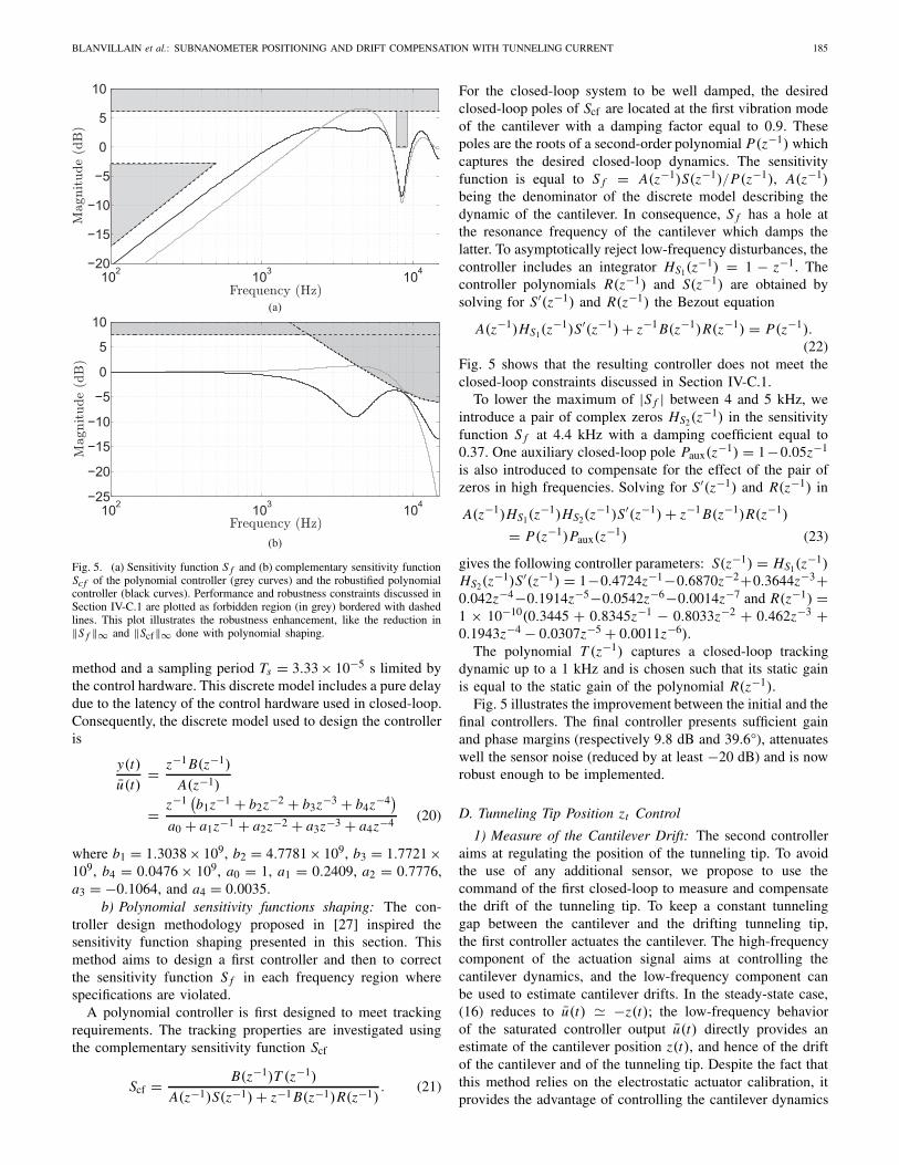
We now translate these objectives into constraints on thesensitivity functions S f and Scf . Notice that the constraints onS f and Scf are plotted as forbidden regions colored in grey onFig. 5. A tracking without error is guaranteed if the sensitivityfunction tends to zero at low frequencies. To increase thetracking accuracy, the closed-loop will damp the resonancefrequency if the sensitivity function S f has a hole below 0 dBat this frequency. Similarly, the effect of the sensor noise isdecreased if S f is below −3 dB in the frequency region werethe noise is dominant, i.e. until 500 Hz. To reject the influenceof the sensor drift on the tunneling gap, S f should be below theinverse of the drift’s frequency response. In our case, it meansthat S f should be below a line increasing by 0.05 dB orderof magnitude per Hertz and crossing 0 dB at 20 Hz (to takeinto consideration the worst case). Regarding the modeling

uncertainties, ez being an input disturbance, its effect can behere asymptotically rejected if the sensitivity function S f tendsto zero at low frequencies. The uncertainty in κ is capturedby the perturbed plant G(s)(1 + �wκ), where |�| ≤ 1 andwκ = 0.7/κ (an uncertainty of ±0.7 Å−1 captures the amountof variation of κ measured during several experiments). It canbe shown that for plants belonging to a class G(s)(1 +�wκ),a controller satisfying ‖Scf‖∞ ≤ ‖κ/0.7‖∞ guarantees theclosed-loop stability [25]. Due to the computing time of thecontrol algorithm, the delay margin is chosen to be at leastequal to one sampling period. In this case, the closed-loopremains stable if ‖Scf ‖∞ ≤ ‖1/s‖∞ [26]. Finally, robustnessis also related to classical gain and phase margins, denotedby GM and PM, respectively. Good values (GM ≥ 6 dBand PM ≥ 30°) can both be guaranteed if ‖S f ‖∞ is < 6 dBat all frequencies [25].

2) Robust Controller Design:a) Controller structure and discrete open-loop model:

A discrete RST-type controller (following the terminology of[27] and [28] for instance), where R(z−1), S(z−1), and T (z−1)are polynomials in z−1 defining the controller, is designedto fulfill performances specifications. Polynomials are writtenin italic capital letters, not to be confused with sensitivityfunctions written only in capital letters. The controller outputu(t) must be positive according to (15). For this purpose, theRST controller includes a saturation, in the sense that thecontroller output without saturation u(t) is defined by

u(t) = T (z−1)r(t) − R(z−1)y(t) − S∗(z−1)u(t − 1)

s0(18)

where s0 + S∗(z−1) = S(z−1). The saturated controller outputu(t) forces the signal to be positive

u(t) ={

u(t), if u(t) > 00, if u(t) ≤ 0

(19)

such that when u(t) is negative, the controller output u(t)saturates. The computation of the controller output considersthe previous saturated values, such that the controller doesnot loose its properties in the presence of the saturation [27].Coefficients of polynomials R(z−1) and S(z−1) are computedon the basis of a discretization of (17), with a zero-order hold


(a)

(b)

Fig. 5. (a) Sensitivity function S f and (b) complementary sensitivity functionScf of the polynomial controller (grey curves) and the robustified polynomialcontroller (black curves). Performance and robustness constraints discussed inSection IV-C.1 are plotted as forbidden region (in grey) bordered with dashedlines. This plot illustrates the robustness enhancement, like the reduction in‖S f ‖∞ and ‖Scf‖∞ done with polynomial shaping.

method and a sampling period Ts = 3.33 × 10−5 s limited bythe control hardware. This discrete model includes a pure delaydue to the latency of the control hardware used in closed-loop.Consequently, the discrete model used to design the controlleris

y(t)

u(t)= z−1 B(z−1)

A(z−1)

= z−1(b1z−1 + b2z−2 + b3z−3 + b4z−4

)a0 + a1z−1 + a2z−2 + a3z−3 + a4z−4 (20)

where b1 = 1.3038 × 109, b2 = 4.7781 × 109, b3 = 1.7721 ×109, b4 = 0.0476 × 109, a0 = 1, a1 = 0.2409, a2 = 0.7776,a3 = −0.1064, and a4 = 0.0035.

b) Polynomial sensitivity functions shaping: The con-troller design methodology proposed in [27] inspired thesensitivity function shaping presented in this section. Thismethod aims to design a first controller and then to correctthe sensitivity function S f in each frequency region wherespecifications are violated.

A polynomial controller is first designed to meet trackingrequirements. The tracking properties are investigated usingthe complementary sensitivity function Scf

Scf = B(z−1)T (z−1)

A(z−1)S(z−1) + z−1 B(z−1)R(z−1). (21)

For the closed-loop system to be well damped, the desiredclosed-loop poles of Scf are located at the first vibration modeof the cantilever with a damping factor equal to 0.9. Thesepoles are the roots of a second-order polynomial P(z−1) whichcaptures the desired closed-loop dynamics. The sensitivityfunction is equal to S f = A(z−1)S(z−1)/P(z−1), A(z−1)being the denominator of the discrete model describing thedynamic of the cantilever. In consequence, S f has a hole atthe resonance frequency of the cantilever which damps thelatter. To asymptotically reject low-frequency disturbances, thecontroller includes an integrator HS1(z

−1) = 1 − z−1. Thecontroller polynomials R(z−1) and S(z−1) are obtained bysolving for S′(z−1) and R(z−1) the Bezout equation

A(z−1)HS1(z−1)S′(z−1) + z−1 B(z−1)R(z−1) = P(z−1).

(22)Fig. 5 shows that the resulting controller does not meet theclosed-loop constraints discussed in Section IV-C.1.

To lower the maximum of |S f | between 4 and 5 kHz, weintroduce a pair of complex zeros HS2(z

−1) in the sensitivityfunction S f at 4.4 kHz with a damping coefficient equal to0.37. One auxiliary closed-loop pole Paux(z−1) = 1−0.05z−1

is also introduced to compensate for the effect of the pair ofzeros in high frequencies. Solving for S′(z−1) and R(z−1) in

A(z−1)HS1(z−1)HS2(z

−1)S′(z−1) + z−1 B(z−1)R(z−1)

= P(z−1)Paux(z−1) (23)

gives the following controller parameters: S(z−1) = HS1(z−1)

HS2(z−1)S′(z−1) = 1−0.4724z−1−0.6870z−2+0.3644z−3+

0.042z−4−0.1914z−5−0.0542z−6−0.0014z−7 and R(z−1) =1 × 10−10(0.3445 + 0.8345z−1 − 0.8033z−2 + 0.462z−3 +0.1943z−4 − 0.0307z−5 + 0.0011z−6).

The polynomial T (z−1) captures a closed-loop trackingdynamic up to a 1 kHz and is chosen such that its static gainis equal to the static gain of the polynomial R(z−1).

Fig. 5 illustrates the improvement between the initial and thefinal controllers. The final controller presents sufficient gainand phase margins (respectively 9.8 dB and 39.6°), attenuateswell the sensor noise (reduced by at least −20 dB) and is nowrobust enough to be implemented.

D. Tunneling Tip Position zt Control

1) Measure of the Cantilever Drift: The second controlleraims at regulating the position of the tunneling tip. To avoidthe use of any additional sensor, we propose to use thecommand of the first closed-loop to measure and compensatethe drift of the tunneling tip. To keep a constant tunnelinggap between the cantilever and the drifting tunneling tip,the first controller actuates the cantilever. The high-frequencycomponent of the actuation signal aims at controlling thecantilever dynamics, and the low-frequency component canbe used to estimate cantilever drifts. In the steady-state case,(16) reduces to u(t) � −z(t); the low-frequency behaviorof the saturated controller output u(t) directly provides anestimate of the cantilever position z(t), and hence of the driftof the cantilever and of the tunneling tip. Despite the fact thatthis method relies on the electrostatic actuator calibration, itprovides the advantage of controlling the cantilever dynamics


102 103 104−185

−180

−175

−170

−165

−160

−155

−150M

agni

tude

(dB

)

Frequency (Hz)

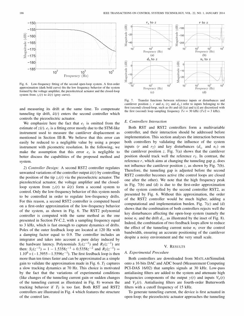
Fig. 6. Low-frequency fitting of the second open-loop system. A first-orderapproximation (dark bold curve) fits the low frequency behavior of the systemformed by the voltage amplifier, the piezolectrical actuator and the closed-loopsystem from zt (t) to u(t) (grey curve).

and measuring its drift at the same time. To compensatetunneling tip drift, u(t) enters the second controller whichcontrols the piezoelectric actuator.

We emphasize here the fact that ez is omitted from theestimate of z(t). ez is a fitting error mostly due to the STM-likeinstrument used to measure the cantilever displacement asmentioned in Section III-B. We believe that this error caneasily be reduced to a negligible value by using a properinstrument with picometric resolution. In the following, wemake the assumption that this error ez is negligible tobetter discuss the capabilities of the proposed method andsystem.

2) Controller Design: A second RST2 controller regulatesunwanted variations of the controller output u(t) by controllingthe position of the tip zt (t) via the piezoelectric actuator. Thepiezolectrical actuator, the voltage amplifier and the closed-loop system from zt (t) to u(t) form a second system tocontrol. Only the low-frequency behavior of this system needsto be controlled in order to regulate low-frequency drifts.For this reason, a second RST2 controller is computed basedon a first-order approximation of the low-frequency behaviorof the system, as shown in Fig. 6. The RST2 polynomialcontroller is computed with the same method as the onepresented in Section IV-C.2, with a sampling frequency equalto 3 kHz, which is fast enough to capture dynamics of drifts.Poles of the outer feedback loop are located at 120 Hz witha damping factor equal to 0.9. The controller includes anintegrator and takes into account a pure delay induced bythe hardware latency. Polynomials S2(z−1) and R2(z−1) arethen: S2(z−1) = 1 − 1.5358z−1 + 0.5358z−2 and R2(z−1) =1.106×(−1.3955−1.5596z−1). The first feedback loop is thenmore than ten times faster and can be approximated as a simplegain to validate the approximation made in Fig. 6. T2 capturesa slow tracking dynamics at 70 Hz. This choice is motivatedby the fact that the variations of experimental conditions(like changes of the tunneling current gain or sudden changesof the tunneling current as illustrated in Fig. 8) worsen thetracking behavior if T2 is too fast. Both RST and RST2controllers are illustrated in Fig. 4 which features the structureof the control law.

(a) (b)

(c) (d)

Fig. 7. Transfer functions between reference inputs or disturbances andcantilever position z. r and ni (r2 and dzt ) refer to inputs belonging to thefirst (second) closed-loop, such as (b) and (d) [(a) and (c)] are discretized withthe first (second) loop sampling frequency T e = 30 kHz (T e2 = 3 kHz).

E. Controllers Interaction

Both RST and RST2 controllers form a multivariablecontroller, and their interaction should be addressed beforeimplementation. This section analyses the interaction betweenboth controllers by validating the influence of the systeminputs (r and r2) and key disturbances (dzt and ni ) onthe cantilever position z. Fig. 7(a) shows that the cantileverposition should track well the reference r2. In contrast, thereference r , which aims at changing the tunneling gap g, doesnot influence the cantilever position z, as shown by Fig. 7(b).Therefore, the tunneling gap is adjusted before the secondRST2 controller becomes active (the control loops are closedone after the other). We note that the high frequency peakin Fig. 7(b) and (d) is due to the first-order approximationof the system controlled by the second controller RST2, aspresented by Fig. 6. Without this approximation, the orderof the RST2 controller would be much higher, adding acomputational and implementation burden. Fig. 7(c) and (d)shows that the combination of both controllers rejects well thekey disturbances affecting the open-loop system (namely thenoise ni and the drift dzt , as illustrated by the inset of Fig. 8).Indeed, the combination of two feedback loops allow to reducethe effect of the tunneling current noise ni over the controlbandwidth, ensuring an accurate positioning of the cantileverdespite a noisy environment and the very small scale.

V. RESULTS

A. Experimental Procedure

Both controllers are downloaded from MATLAB/Simulinkonto a 16 bits DAC and ADC board (Measurement ComputingPCI-DAS 16/02) that samples signals at 30 kHz. Low-passantialiasing filters are added to the system and attenuate highfrequencies components of the output y(t) and inputs Va(t)and Vp(t). Antialiasing filters are fourth-order Butterworthfilters with a cutoff frequency of 15 kHz.

To generate tunneling current, the device is first actuated inopen-loop; the piezoelectric actuator approaches the tunneling


(a) (b)

(c)

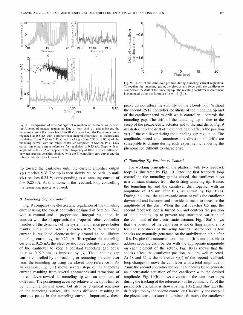
Fig. 8. Comparison of different types of regulation of the tunneling current.(a) Attempt of manual regulation. Due to both drift dzt and noise ni , thetunneling current fluctuates from 0 to 10 V in open loop. (b) Tunneling currentregulated at 0.5 nA with a proportional integral controller. (c) Electrostaticregulation (from 7.85 to 7.95 s) and tracking (from 7.95 to 8.05 s) of thetunneling current with the robust controller computed in Section IV-C. Greycurve: tunneling current reference for regulation is 0.25 nA. Steps with anamplitude of 0.25 nA are applied with a frequency of 100 Hz. Inset: differencebetween spectral densities obtained with the PI controller (grey curve) and therobust controller (black curve).

tip toward the cantilever until the current amplifier outputy(t) reaches 5 V. The tip is then slowly pulled back up untily(t) reaches 0.25 V, corresponding to a tunneling current ofi = 0.25 nA. At this moment, the feedback loop controllingthe tunneling gap g is closed.

B. Tunneling Gap g Control

Fig. 8 compares the electrostatic regulation of the tunnelingcurrent using the robust controller designed in Section IV-Cwith a manual and a proportional integral regulation. Incontrast with the PI approach, the proposed robust controllerhandles all the dynamics of the system, and hence gives betterresults in regulation. When y reaches 0.25 V, the tunnelingcurrent is regulated electrostatically around an equilibriumtunneling current ieq = 0.25 nA. To regulate the tunnelingcurrent at 0.25 nA, the electrostatic force actuates the positionof the cantilever to keep a constant tunneling gap equalto g = 0.929 nm, as imposed by (3). The tunneling gapcan be controlled by approaching or retracting the cantileverfrom the tunneling tip using the closed-loop reference r . Asan example, Fig. 8(c) shows several steps of the tunnelingcurrent, resulting from several approaches and retractions ofthe cantilever toward the tunneling tip with an amplitude of0.029 nm. The positioning accuracy relative to the tip is limitedby tunneling current noise, but also by chemical reactionson the tunneling surface, like atoms diffusion, resulting inspurious peaks in the tunneling current. Importantly, these

0 5 10 15 20−2

−1.5

−1

−0.5

0

Dri

ftof

the

cant

ileve

rpo

siti

onz

(nm

)

Time (sec)

Fig. 9. Drift of the cantilever position during tunneling current regulation.To regulate the tunneling gap g, the electrostatic force pulls the cantilever tocompensate the drift of the tunneling tip. The resulting cantilever displacementis computed using the formula z(t) = −bV 2

a (t).

peaks do not affect the stability of the closed-loop. Withoutthe second RST2 controller, positions of the tunneling tip andof the cantilever tend to drift while controller 1 controls thetunneling gap. The drift of the tunneling tip is due to thecreep of the piezoelectric actuator and to thermal drifts. Fig. 9illustrates how the drift of the tunneling tip affects the positionz(t) of the cantilever during the tunneling gap regulation. Theamplitude, speed and sometimes the direction of drifts aresusceptible to change during each experiments, rendering thephenomenon difficult to characterize.

C. Tunneling Tip Position zt Control

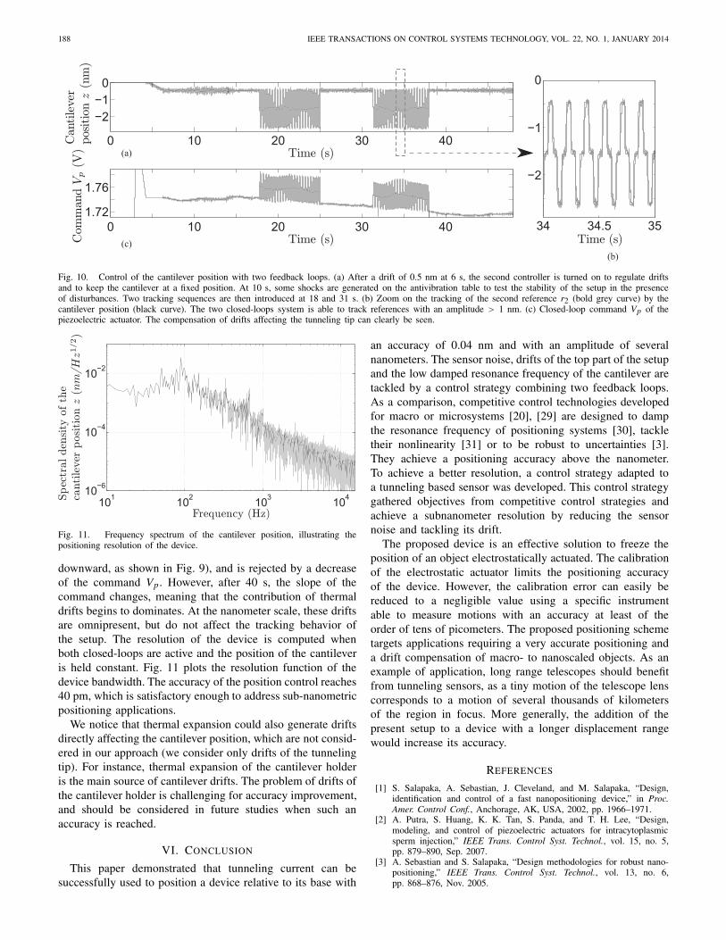
The working principle of the platform with two feedbackloops is illustrated by Fig. 10. Once the first feedback loopcontrolling the tunneling gap is closed, the cantilever staysat a constant distance from the drifting tunneling tip. Hence,the tunneling tip and the cantilever drift together with anamplitude of 0.5 nm after 6 s, as shown by Fig. 10(a).During this time, the electrostatic actuator pulls the cantileverdownward and its command provides a mean to measure theamplitude of the drift. When the drift reaches 0.5 nm, thesecond feedback loop is turned on, and controls the positionof the tunneling tip to prevent any unwanted variation ofthe command of the electrostatic actuator. Fig. 10(a) showsthat the position of the cantilever is not drifting anymore. Totest the robustness of the setup toward disturbances, a fewshocks are manually generated on the antivibration table after10 s. Despite this unconventional method (it is not possible toaddress separate disturbances with the appropriate magnitudeon each element of the setup), Fig. 10(a) shows that theshocks affect the cantilever position, but are well rejected.At 18 and 31 s, the reference r2(t) of the second feedbackloop changes to move the cantilever with a total amplitude of2 nm: the second controller moves the tunneling tip to generatean electrostatic actuation of the cantilever with the desiredamplitude. Fig. 10(b) shows a zoom on the cantilever stepsduring the tracking of the reference r2. The command Vp of thepiezoelectric actuator is shown by Fig. 10(c), and illustrates thedrift rejection by the second controller. Classically, the creep ofthe piezoelectric actuator is dominant (it moves the cantilever


(a)

(b)(c)

Fig. 10. Control of the cantilever position with two feedback loops. (a) After a drift of 0.5 nm at 6 s, the second controller is turned on to regulate driftsand to keep the cantilever at a fixed position. At 10 s, some shocks are generated on the antivibration table to test the stability of the setup in the presenceof disturbances. Two tracking sequences are then introduced at 18 and 31 s. (b) Zoom on the tracking of the second reference r2 (bold grey curve) by thecantilever position (black curve). The two closed-loops system is able to track references with an amplitude > 1 nm. (c) Closed-loop command Vp of thepiezoelectric actuator. The compensation of drifts affecting the tunneling tip can clearly be seen.

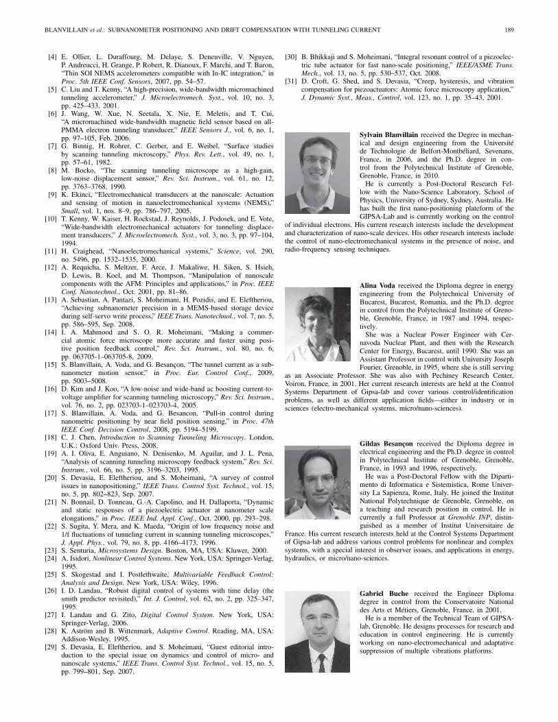
Fig. 11. Frequency spectrum of the cantilever position, illustrating thepositioning resolution of the device.

downward, as shown in Fig. 9), and is rejected by a decreaseof the command Vp . However, after 40 s, the slope of thecommand changes, meaning that the contribution of thermaldrifts begins to dominates. At the nanometer scale, these driftsare omnipresent, but do not affect the tracking behavior ofthe setup. The resolution of the device is computed whenboth closed-loops are active and the position of the cantileveris held constant. Fig. 11 plots the resolution function of thedevice bandwidth. The accuracy of the position control reaches40 pm, which is satisfactory enough to address sub-nanometricpositioning applications.

We notice that thermal expansion could also generate driftsdirectly affecting the cantilever position, which are not consid-ered in our approach (we consider only drifts of the tunnelingtip). For instance, thermal expansion of the cantilever holderis the main source of cantilever drifts. The problem of drifts ofthe cantilever holder is challenging for accuracy improvement,and should be considered in future studies when such anaccuracy is reached.

VI. CONCLUSION

This paper demonstrated that tunneling current can besuccessfully used to position a device relative to its base with

an accuracy of 0.04 nm and with an amplitude of severalnanometers. The sensor noise, drifts of the top part of the setupand the low damped resonance frequency of the cantilever aretackled by a control strategy combining two feedback loops.As a comparison, competitive control technologies developedfor macro or microsystems [20], [29] are designed to dampthe resonance frequency of positioning systems [30], tackletheir nonlinearity [31] or to be robust to uncertainties [3].They achieve a positioning accuracy above the nanometer.To achieve a better resolution, a control strategy adapted toa tunneling based sensor was developed. This control strategygathered objectives from competitive control strategies andachieve a subnanometer resolution by reducing the sensornoise and tackling its drift.

The proposed device is an effective solution to freeze theposition of an object electrostatically actuated. The calibrationof the electrostatic actuator limits the positioning accuracyof the device. However, the calibration error can easily bereduced to a negligible value using a specific instrumentable to measure motions with an accuracy at least of theorder of tens of picometers. The proposed positioning schemetargets applications requiring a very accurate positioning anda drift compensation of macro- to nanoscaled objects. As anexample of application, long range telescopes should benefitfrom tunneling sensors, as a tiny motion of the telescope lenscorresponds to a motion of several thousands of kilometersof the region in focus. More generally, the addition of thepresent setup to a device with a longer displacement rangewould increase its accuracy.

REFERENCES

[1] S. Salapaka, A. Sebastian, J. Cleveland, and M. Salapaka, “Design,identification and control of a fast nanopositioning device,” in Proc.Amer. Control Conf., Anchorage, AK, USA, 2002, pp. 1966–1971.

[2] A. Putra, S. Huang, K. K. Tan, S. Panda, and T. H. Lee, “Design,modeling, and control of piezoelectric actuators for intracytoplasmicsperm injection,” IEEE Trans. Control Syst. Technol., vol. 15, no. 5,pp. 879–890, Sep. 2007.

[3] A. Sebastian and S. Salapaka, “Design methodologies for robust nano-positioning,” IEEE Trans. Control Syst. Technol., vol. 13, no. 6,pp. 868–876, Nov. 2005.


[4] E. Ollier, L. Duraffourg, M. Delaye, S. Deneuville, V. Nguyen,P. Andreucci, H. Grange, P. Robert, R. Dianoux, F. Marchi, and T. Baron,“Thin SOI NEMS accelerometers compatible with In-IC integration,” inProc. 5th IEEE Conf. Sensors, 2007, pp. 54–57.

[5] C. Liu and T. Kenny, “A high-precision, wide-bandwidth micromachinedtunneling accelerometer,” J. Microelectromech. Syst., vol. 10, no. 3,pp. 425–433, 2001.

[6] J. Wang, W. Xue, N. Seetala, X. Nie, E. Meletis, and T. Cui,“A micromachined wide-bandwidth magnetic field sensor based on all-PMMA electron tunneling transducer,” IEEE Sensors J., vol. 6, no. 1,pp. 97–105, Feb. 2006.

[7] G. Binnig, H. Rohrer, C. Gerber, and E. Weibel, “Surface studiesby scanning tunneling microscopy,” Phys. Rev. Lett., vol. 49, no. 1,pp. 57–61, 1982.

[8] M. Bocko, “The scanning tunneling microscope as a high-gain,low-noise displacement sensor,” Rev. Sci. Instrum., vol. 61, no. 12,pp. 3763–3768, 1990.

[9] K. Ekinci, “Electromechanical transducers at the nanoscale: Actuationand sensing of motion in nanoelectromechanical systems (NEMS),”Small, vol. 1, nos. 8–9, pp. 786–797, 2005.

[10] T. Kenny, W. Kaiser, H. Rockstad, J. Reynolds, J. Podosek, and E. Vote,“Wide-bandwidth electromechanical actuators for tunneling displace-ment transducers,” J. Microelectromech. Syst., vol. 3, no. 3, pp. 97–104,1994.

[11] H. Craighead, “Nanoelectromechanical systems,” Science, vol. 290,no. 5496, pp. 1532–1535, 2000.

[12] A. Requicha, S. Meltzer, F. Arce, J. Makaliwe, H. Siken, S. Hsieh,D. Lewis, B. Koel, and M. Thompson, “Manipulation of nanoscalecomponents with the AFM: Principles and applications,” in Proc. IEEEConf. Nanotechnol., Oct. 2001, pp. 81–86.

[13] A. Sebastian, A. Pantazi, S. Moheimani, H. Pozidis, and E. Eleftheriou,“Achieving subnanometer precision in a MEMS-based storage deviceduring self-servo write process,” IEEE Trans. Nanotechnol., vol. 7, no. 5,pp. 586–595, Sep. 2008.

[14] I. A. Mahmood and S. O. R. Moheimani, “Making a commer-cial atomic force microscope more accurate and faster using posi-tive position feedback control,” Rev. Sci. Instrum., vol. 80, no. 6,pp. 063705-1–063705-8, 2009.

[15] S. Blanvillain, A. Voda, and G. Besançon, “The tunnel current as a sub-nanometer motion sensor,” in Proc. Eur. Control Conf., 2009,pp. 5003–5008.

[16] D. Kim and J. Koo, “A low-noise and wide-band ac boosting current-to-voltage amplifier for scanning tunneling microscopy,” Rev. Sci. Instrum.,vol. 76, no. 2, pp. 023703-1–023703-4, 2005.

[17] S. Blanvillain, A. Voda, and G. Besancon, “Pull-in control duringnanometric positioning by near field position sensing,” in Proc. 47thIEEE Conf. Decision Control, 2008, pp. 5194–5199.

[18] C. J. Chen, Introduction to Scanning Tunneling Microscopy. London,U.K.: Oxford Univ. Press, 2008.

[19] A. I. Oliva, E. Anguiano, N. Denisenko, M. Aguilar, and J. L. Pena,“Analysis of scanning tunneling microscopy feedback system,” Rev. Sci.Instrum., vol. 66, no. 5, pp. 3196–3203, 1995.

[20] S. Devasia, E. Eleftheriou, and S. Moheimani, “A survey of controlissues in nanopositioning,” IEEE Trans. Control Syst. Technol., vol. 15,no. 5, pp. 802–823, Sep. 2007.

[21] N. Bonnail, D. Tonneau, G.-A. Capolino, and H. Dallaporta, “Dynamicand static responses of a piezoelectric actuator at nanometer scaleelongations,” in Proc. IEEE Ind. Appl. Conf., Oct. 2000, pp. 293–298.

[22] S. Sugita, Y. Mera, and K. Maeda, “Origin of low frequency noise and1/f fluctuations of tunneling current in scanning tunneling microscopes,”J. Appl. Phys., vol. 79, no. 8, pp. 4166–4173, 1996.

[23] S. Senturia, Microsystems Design. Boston, MA, USA: Kluwer, 2000.[24] A. Isidori, Nonlinear Control Systems. New York, USA: Springer-Verlag,

1995.[25] S. Skogestad and I. Postlethwaite, Multivariable Feedback Control:

Analysis and Design. New York, USA: Wiley, 1996.[26] I. D. Landau, “Robust digital control of systems with time delay (the

smith predictor revisited),” Int. J. Control, vol. 62, no. 2, pp. 325–347,1995.

[27] I. Landau and G. Zito, Digital Control System. New York, USA:Springer-Verlag, 2006.

[28] K. Aström and B. Wittenmark, Adaptive Control. Reading, MA, USA:Addison-Wesley, 1995.

[29] S. Devasia, E. Eleftheriou, and S. Moheimani, “Guest editorial intro-duction to the special issue on dynamics and control of micro- andnanoscale systems,” IEEE Trans. Control Syst. Technol., vol. 15, no. 5,pp. 799–801, Sep. 2007.

[30] B. Bhikkaji and S. Moheimani, “Integral resonant control of a piezoelec-tric tube actuator for fast nano-scale positioning,” IEEE/ASME Trans.Mech., vol. 13, no. 5, pp. 530–537, Oct. 2008.

[31] D. Croft, G. Shed, and S. Devasia, “Creep, hysteresis, and vibrationcompensation for piezoactuators: Atomic force microscopy application,”J. Dynamic Syst., Meas., Control, vol. 123, no. 1, pp. 35–43, 2001.

Sylvain Blanvillain received the Degree in mechan-ical and design engineering from the Universitéde Technologie de Belfort-Montbéliard, Sevenans,France, in 2006, and the Ph.D. degree in con-trol from the Polytechnical Institute of Grenoble,Grenoble, France, in 2010.

He is currently a Post-Doctoral Research Fel-low with the Nano-Science Laboratory, School ofPhysics, University of Sydney, Sydney, Australia. Hehas built the first nano-positioning plateform of theGIPSA-Lab and is currently working on the control

of individual electrons. His current research interests include the developmentand characterization of nano-scale devices. His other research interests includethe control of nano-electromechanical systems in the presence of noise, andradio-frequency sensing techniques.

Alina Voda received the Diploma degree in energyengineering from the Polytechnical University ofBucarest, Bucarest, Romania, and the Ph.D. degreein control from the Polytechnical Institute of Greno-ble, Grenoble, France, in 1987 and 1994, respec-tively.

She was a Nuclear Power Engineer with Cer-navoda Nuclear Plant, and then with the ResearchCenter for Energy, Bucarest, until 1990. She was anAssistant Professor in control with University JosephFourier, Grenoble, in 1995, where she is still serving

as an Associate Professor. She was also with Pechiney Research Center,Voiron, France, in 2001. Her current research interests are held at the ControlSystems Department of Gipsa-lab and cover various control/identificationproblems, as well as different application fields—either in industry or insciences (electro-mechanical systems, micro/nano-sciences).

Gildas Besançon received the Diploma degree inelectrical engineering and the Ph.D. degree in controlin Polytechnical Institute of Grenoble, Grenoble,France, in 1993 and 1996, respectively.

He was a Post-Doctoral Fellow with the Diparti-mento di Informatica e Sistemistica, Rome Univer-sity La Sapienza, Rome, Italy. He joined the InstitutNational Polytechnique de Grenoble, Grenoble, ona teaching and research position in control. He iscurrently a full Professor at Grenoble INP, distin-guished as a member of Institut Universitaire de

France. His current research interests held at the Control Systems Departmentof Gipsa-lab and address various control problems for nonlinear and complexsystems, with a special interest in observer issues, and applications in energy,hydraulics, or micro/nano-sciences.

Gabriel Buche received the Engineer Diplomadegree in control from the Conservatoire Nationaldes Arts et Métiers, Grenoble, France, in 2001.

He is a member of the Technical Team of GIPSA-lab, Grenoble. He designs processes for research andeducation in control engineering. He is currentlyworking on nano-electromechanical and adaptativesuppression of multiple vibrations platforms.

Documents

Subnanometer Positioning and Drift Compensation With Tunneling Current