Embed Size (px)
Citation preview
Suche nach Kaluza-Klein Dunkle Materie Kandidaten
mit dem CDMS Experiment
-
Searching for Kaluza-Klein Dark Matter Candidates
with the CDMS experiment
von
Sebastian Arrenberg
Diplomarbeit in PHYSIKvorgelegt der
Fakultat fur Mathematik, Informatik und Naturwissenschaftender RWTH Aachen
im Oktober 2007
angefertigt im
I. Physikalischen Institut der RWTH AachenProf. Dr. Laura Baudis
October 2, 2007

Contents
1 Introduction 1
2 UEDs - Theoretical Background 32.1 Special Relativity . . . . . . . . . . . . . . . . . . . . . . . . . . . . 32.2 General Relativity . . . . . . . . . . . . . . . . . . . . . . . . . . . 62.3 Kaluza-Klein Theory . . . . . . . . . . . . . . . . . . . . . . . . . 112.4 The Compactification of Extra Dimensions . . . . . . . . . . . . . 152.5 Universal Extra Dimensions . . . . . . . . . . . . . . . . . . . . . . 20
3 Cross sections of the B(1) and nuclei 31
4 Form factors 464.1 Spin-independent form factors . . . . . . . . . . . . . . . . . . . . . 474.2 Spin-dependent form factors . . . . . . . . . . . . . . . . . . . . . . 49
5 Event rates from B(1)-nuclei scattering 63
6 Annual modulation 84
7 Limits on cross sections and WIMP-nucleon couplings 937.1 Limits on spin-independent cross sections . . . . . . . . . . . . . . 937.2 Limits on spin-dependent WIMP-nucleon couplings and cross sections101
8 Conclusion 123
A Spin-independent cross sections 125A.1 Spin-independent cross sections for fixed mH . . . . . . . . . . . . 125A.2 Spin-independent cross sections for fixed ∆ . . . . . . . . . . . . . 128
B Event rates 131B.1 Differential event rates for various values of ∆ . . . . . . . . . . . . 131B.2 Spin-dependent differential event rates . . . . . . . . . . . . . . . . 133B.3 Total event rates for various values of ∆ . . . . . . . . . . . . . . . 135B.4 Total event rates for negligible threshold . . . . . . . . . . . . . . . 137
i
ii CONTENTS
C Limits on cross sections and WIMP-nucleon couplings 138C.1 Limits on spin-independent cross sections using the Optimum In-
terval method . . . . . . . . . . . . . . . . . . . . . . . . . . . . . . 138C.2 θ scan for the spin-dependent form factor of 129Xe using the Ni-
jmegen II method . . . . . . . . . . . . . . . . . . . . . . . . . . . . 141C.3 θ scan for the spin-dependent differential event rates of 129Xe using
the Nijmegen II method . . . . . . . . . . . . . . . . . . . . . . . . 146C.4 Combined limits on WIMP-nucleon couplings for different ∆s . . . 151C.5 Comparison of limits on WIMP-nucleon couplings from the xenon
isotopes using the Bonn A and the Nijmegen II method . . . . . . 153C.6 Supersymmetry . . . . . . . . . . . . . . . . . . . . . . . . . . . . . 154
Acknowledgement 158
Statement 159
List of Figures
2.1 5-dimensional space time . . . . . . . . . . . . . . . . . . . . . . . . 162.2 Orbifold compactification . . . . . . . . . . . . . . . . . . . . . . . 192.3 Allowed and forbidden vertices in the UED model . . . . . . . . . 232.4 Mass spectrum of level one Kaluza-Klein particles . . . . . . . . . 242.5 Weinberg angle for the first five Kaluza-Klein modes . . . . . . . . 252.6 Relic density of the B(1) . . . . . . . . . . . . . . . . . . . . . . . . 29
3.1 B(1)-quark scattering via Higgs boson exchange . . . . . . . . . . . 343.2 B(1)-quark scattering via q(1) exchange . . . . . . . . . . . . . . . . 353.3 Spin-independent B(1)-neutron cross sections for mH = 120 GeV . 383.4 Spin-independent B(1)-neutron cross sections for ∆ = 0.15 . . . . . 393.5 Spin-independent B(1)-neutron cross sections for mB(1) = 500 GeV 403.6 Spin-dependent B(1)-proton cross sections . . . . . . . . . . . . . . 433.7 Spin-dependent B(1)-neutron cross sections . . . . . . . . . . . . . 44
4.1 Spin-independent form factors of 28Si, 73Ge and 131Xe . . . . . . . 484.2 Spin structure functions of 29Si . . . . . . . . . . . . . . . . . . . . 524.3 Spin structure functions of 73Ge . . . . . . . . . . . . . . . . . . . . 544.4 Spin structure functions of 129Xe using the Bonn A method . . . . 564.5 Spin structure functions of 129Xe using the Nijmegen II method . . 564.6 Spin structure functions of 131Xe using the Bonn A method . . . . 574.7 Spin structure functions of 131Xe using the Nijmegen II method . . 574.8 Spin structure functions of 131Xe using the QTDA method . . . . . 594.9 Squared spin-dependent form factors for 129Xe and 131Xe . . . . . 604.10 Silicon form factors . . . . . . . . . . . . . . . . . . . . . . . . . . . 614.11 Germanium form factors . . . . . . . . . . . . . . . . . . . . . . . . 624.12 Xenon form factors . . . . . . . . . . . . . . . . . . . . . . . . . . . 62
5.1 Motion of the earth around the sun . . . . . . . . . . . . . . . . . . 645.2 Dependence of vE on the day in a year . . . . . . . . . . . . . . . . 665.3 Dependence of vmax on the scattering angle in the galactic rest frame 685.4 Dependence of 〈ERmax〉 on the WIMP mass . . . . . . . . . . . . . 705.5 Spin-independent differential event rates for B(1)-73Ge scattering . 755.6 Spin-dependent differential event rates for B(1)-73Ge scattering . . 76
iii
iv LIST OF FIGURES
5.7 Comparison of differential event rates scattering from various targetnuclei . . . . . . . . . . . . . . . . . . . . . . . . . . . . . . . . . . 77
5.8 Differential event rates for B(1)-Si scattering . . . . . . . . . . . . . 775.9 Differential event rates for B(1)-Ge scattering . . . . . . . . . . . . 785.10 Differential event rates for B(1)-Xe scattering . . . . . . . . . . . . 785.11 Comparison of total event rates scattering from various target nuclei 805.12 Total event rates for B(1)-Si scattering . . . . . . . . . . . . . . . . 805.13 Total event rates for B(1)-Ge scattering . . . . . . . . . . . . . . . 815.14 Total event rates for B(1)-Xe scattering . . . . . . . . . . . . . . . 815.15 Differential event rates for very low masses . . . . . . . . . . . . . 83
6.1 Differential Event rates for June 2nd and December 2nd consideringmB(1) = 30 GeV . . . . . . . . . . . . . . . . . . . . . . . . . . . . 85
6.2 Differential Event rates for June 2nd and December 2nd consideringmB(1) = 200 GeV . . . . . . . . . . . . . . . . . . . . . . . . . . . . 85
6.3 Differential Event rates for June 2nd and December 2nd consideringmB(1) = 1000 GeV . . . . . . . . . . . . . . . . . . . . . . . . . . . 86
6.4 Time dependence of the total event rate considering mB(1) = 30 GeV 866.5 Time dependence of the total event rate considering mB(1) = 200 GeV 876.6 Time dependence of the total event rate consideringmB(1) = 1000 GeV 876.7 Computing the crossover recoil energy . . . . . . . . . . . . . . . . 896.8 Mass dependence of the crossover recoil energy for 28Si, 73Ge and
131Xe . . . . . . . . . . . . . . . . . . . . . . . . . . . . . . . . . . . 896.9 Computing the crossover recoil energy . . . . . . . . . . . . . . . . 916.10 Mass dependence of the crossover recoil energy for 28Si, 73Ge and
131Xe . . . . . . . . . . . . . . . . . . . . . . . . . . . . . . . . . . . 916.11 Dependence of the differential event rate on v0 . . . . . . . . . . . 92
7.1 Spin-independent cross section limits from silicon detectors used byCDMS . . . . . . . . . . . . . . . . . . . . . . . . . . . . . . . . . . 99
7.2 Spin-independent cross section limits from germanium detectorsused by CDMS . . . . . . . . . . . . . . . . . . . . . . . . . . . . . 99
7.3 Spin-independent cross section limits from XENON10 . . . . . . . 1007.4 Comparison of spin-independent cross section limits . . . . . . . . 1007.5 Testing a substitution . . . . . . . . . . . . . . . . . . . . . . . . . 1057.6 Spin-dependent cross section limits from 29Si considering pure cou-
pling to neutrons . . . . . . . . . . . . . . . . . . . . . . . . . . . . 1147.7 Spin-dependent cross section limits from 29Si considering pure cou-
pling to protons. . . . . . . . . . . . . . . . . . . . . . . . . . . . . 1147.8 Spin-dependent cross section limits from 73Ge considering pure cou-
pling to neutrons . . . . . . . . . . . . . . . . . . . . . . . . . . . . 1157.9 Spin-dependent cross section limits from 73Ge considering pure cou-
pling to protons. . . . . . . . . . . . . . . . . . . . . . . . . . . . . 115
LIST OF FIGURES v
7.10 Spin-dependent cross section limits from 129Xe and 131Xe consider-ing pure coupling to neutrons . . . . . . . . . . . . . . . . . . . . . 116
7.11 Spin-dependent cross section limits from 129Xe and 131Xe consider-ing pure coupling to protons . . . . . . . . . . . . . . . . . . . . . . 116
7.12 Comparison of spin-dependent cross section limits considering purecoupling to neutrons . . . . . . . . . . . . . . . . . . . . . . . . . . 117
7.13 Comparison of spin-dependent cross section limits considering purecoupling to protons . . . . . . . . . . . . . . . . . . . . . . . . . . . 117
7.14 Comparison of spin-dependent cross section limits from XENON10considering pure coupling to neutrons and using different spin struc-ture functions . . . . . . . . . . . . . . . . . . . . . . . . . . . . . . 118
7.15 Comparison of spin-dependent cross section limits from XENON10considering pure coupling to protons and using different spin struc-ture functions . . . . . . . . . . . . . . . . . . . . . . . . . . . . . . 118
7.16 Comparison of spin-dependent cross section limits from XENON10considering pure coupling to neutrons and using different spin struc-ture functions . . . . . . . . . . . . . . . . . . . . . . . . . . . . . . 119
7.17 Comparison of spin-dependent cross section limits from XENON10considering pure coupling to protons and using different spin struc-ture functions . . . . . . . . . . . . . . . . . . . . . . . . . . . . . . 119
7.18 Limits on WIMP-nucleon couplings from 29Si . . . . . . . . . . . . 1207.19 Limits on WIMP-nucleon couplings from 73Ge . . . . . . . . . . . . 1207.20 Limits on WIMP-nucleon couplings from 129Xe . . . . . . . . . . . 1217.21 Limits on WIMP-nucleon couplings from 131Xe . . . . . . . . . . . 1217.22 Limits on WIMP-nucleon couplings from 73Ge comparing different
∆s . . . . . . . . . . . . . . . . . . . . . . . . . . . . . . . . . . . . 1227.23 Combined limits on WIMP-nucleon couplings . . . . . . . . . . . . 122
List of Tables
3.1 Quark properties . . . . . . . . . . . . . . . . . . . . . . . . . . . . 343.2 Hadronic matrix elements . . . . . . . . . . . . . . . . . . . . . . . 363.3 Matrix elements of the quark axial-vector current . . . . . . . . . . 423.4 Target isotopes used by CDMS and XENON10 . . . . . . . . . . . 45
4.1 Values for 〈Sp〉, 〈Sn〉 and µ for all considered isotopes . . . . . . . 534.2 Coefficients used in the fits of the spin structure functions for 129Xe
and 131Xe applying the Bonn A and the Nijmegen II method . . . 554.3 Values related to the fits of the spin structure functions for 131Xe
applying the QTDA method . . . . . . . . . . . . . . . . . . . . . . 59
5.1 Facts about CDMS and XENON10 . . . . . . . . . . . . . . . . . . 74
7.1 Events in CDMS and XENON10 . . . . . . . . . . . . . . . . . . . 957.2 Minimum spin-independent cross section limits . . . . . . . . . . . 1017.3 Minimum spin-dependent cross section limits . . . . . . . . . . . . 109
vi
Chapter 1
Introduction
The determination of the nature of dark matter which is one of the most impor-tant ingredients of the universe considering the evolution of its structure remainsamong the most important questions in astrophysics. Though there are severalproposals available in the literature to solve this problem the most promising can-didate is a Weakly Interacting Massive Particle or WIMP. The most extensivelystudied candidate is the neutralino arising from a supersymmetric extension of thestandard model. However there are several other theories giving rise to appropri-ate candidates like the model of Universal Extra Dimensions which drew a lot ofattention recently.
It is this model which is investigated in great detail in this diploma thesiswith special emphasis on the direct detection of the B(1) which is supposed tobe the lightest stable particle arising from this theory. Theoretical predictionson its cross sections are investigated considering both spin-independent and spin-dependent interactions. Moreover predictions on differential and total event ratesare computed as well. Finally limits on the cross sections and WIMP-nucleoncouplings are analyzed using data from the CDMS and XENON10 experiments.
Both experiments are so-called direct detection experiments which seek to mea-sure the energy deposited when a WIMP interacts with a nucleus in the detector.
For example CDMS is an experiment using semiconductor crystals which arecooled down to a temperature of a few millikelvin. Avoiding unwanted backgroundin these experiments is usually one of the most important subjects. Therefor theyare usually installed deep underground and surrounded by shields of lead andpolyethylene.
CDMS uses so-called ZIP (=Z-sensitive Ionization and Phonon) detectors inorder to discriminate between electron recoils which constitute most of the back-ground and nuclear recoils arising from neutrons and hopefully WIMPs on anevent-by-event basis by simultaniously measuring an ionization and a phonon sig-nal. Moreover the detectors also provide timing information which can be used toreject surface events. These events are problematic since they yield poor ionizationcollection and hence mimic nuclear recoils.
1
2 CHAPTER 1. INTRODUCTION
The used data from CDMS was obtained during the run 118 from October 11,2003 until January 11, 2004 and the run 119 from March 25, 2004 to August 8,2004 using two towers each with 6 detectors. The data from XENON10 was takenbetween October 6, 2006 and February 14, 2007.
Chapter 2
UEDs - TheoreticalBackground
In everyday life people experience the existence of only three space dimensionsand of course one time dimension. Since this seems to be so natural the questionarises why physicists consider additional dimensions at all. To understand thesethoughts it is the best to start with the first occurance of extra dimensions in theliterature which means taking a look at the work of Theodor Kaluza and OscarKlein1 who released their determinations intended to combine General Relativityand Electrodynamics in the 20s of the last century only a few years after AlbertEinstein developed General Relativity.
So since General Relativity plays such a crucial role in the context of extradimensions this chapter is about to start with a short introduction to SpecialRelativity and this intellectual masterpiece.
2.1 Special Relativity
In 1905 Albert Einstein published Special Relativity a theory based on two mainconcepts:
• The special principle of relativityAll laws of physics remain the same in all inertial frames which means thatno privileged frames of reference exist.
• Invariance of the speed of lightThe speed of light in a vacuum is a universal constant which is especiallyindependent of the motion of the source.
1In fact there even was an earlier attempt by Nordstrom in 1914 but this efford did notachieve so much attention especialy because he used his own (wrong) theory of Gravitation.Anyway Kaluza and Klein were influenced by his work.
3
4 CHAPTER 2. UEDS - THEORETICAL BACKGROUND
The resulting concept revolutionized physics by combining space and time into afour-dimensional vector space the so-called Minkowski space breaking down theidea of an absolute time. In this Minkowski space the differential of distance dsis given by
ds2 = dt2 − d~r 2 = ηαβ dxαdxβ (2.1)
with the metric
ηαβ =
+1 0 0 00 −1 0 00 0 −1 00 0 0 −1
. (2.2)
The fact that all of its components are constant reflects that the space consideredin Special Relativity is flat.
One of the most important improvements was the replacement of Galilei trans-formations with Lorentz transformations switching from one inertial frame to an-other one. So physical laws need to be expressed in a new form reflecting theirabidance to Lorentz invariance. In other words they have to be written as a ten-sor equation. For example Electrodynamics which will be discussed in more detailbelow is a theory which is intrinsically covariant. Other theories however are notwhich means that they have to be generalized to fit in the frame work of SpecialRelativity.
Consider for example a pointlike particle of mass m neglecting all forces. ThenNewton’s Law yields
md~vdt
= ~0 (2.3)
which is easily generalized to
mduα
dτ= 0 (2.4)
where
uα =dxα
dτ(2.5)
is the four velocity and τ a quantity parameterizing the world line of the particlefor example the proper time in the case that it is not massless.
This equation is correct because it is covariant and yields (2.3) in the non-relativistic limit. In fact these two conditions generally define the way theoriesare made relativistic.
2.1. SPECIAL RELATIVITY 5
In the case that forces have an impact on the particle a force ~F in (2.3) andFα in (2.4) has to be introduced on the right side of these equations. An examplewill be given immediately.
Finding a form for Electrodynamics which is invariant under Lorentz trans-formations is a quite easy task because the Maxwell equations are covariant bydesign. This can be shown by introducing the antisymmetric field strength tensor
Fαβ = ∂αAβ − ∂βAα =
0 −EX −EY −EZEX 0 −BZ BYEY BZ 0 −BXEZ −BY BX 0
(2.6)
with the gauge potential Aα and the components of the elecrtric field Ei and theMagnetic Field Bi. Now the homogenous and inhomogeneous Maxwell equationscan be written as
εαβγδ∂βFγδ = 0 (2.7)
and
∂αFαβ = 4πjβ (2.8)
respectively which are manifest covariant and where the fully antisymmetricLevi-Civita-Pseudotensor ε has been introduced. Using this convention the equa-tion of motion for a pointlike particle with charge q is given by
mduα
dτ= qFαβuβ . (2.9)
Again the validity can be checked by showing that this equation yields the knownnon-relativistic result. Moreover the energy-momemtum tensor
Tαβ =1
4π
(FαγF
γβ +14ηαβFγδF
γδ
)(2.10)
is of importance considering Generel Relativity because due to the mass energyequivalence it occurs as a source term in Einstein’s field equation.
After finishing his Special Relativity Einstein continued his work trying to finda covariant form for Newton’s theory of Gravitation which is basically given bythe equation of motion for a pointlike particle with mass m
md2~r
dt2= −m∇φ(~r) (2.11)
6 CHAPTER 2. UEDS - THEORETICAL BACKGROUND
and the field equation for the gravitational potential φ
4φ(~r) = 4πGρ(~r) (2.12)
where the matter density ρ appears as the source of φ. These equations look verysimilar to the field equation of Electrostatics and the corresponding non-relativisticequation of motion of a charged particle given by
4φel(~r) = −4πρel(~r) and md2~r
dt2= −q∇φel(~r) (2.13)
respectively. However the underlying truth is much more complicated. This canbe seen by realizing that the source ρel transforms like the 0-component of afour-vector (the current jα) whereas ρ transforms like the 00-component of aLorentztensor namely the energy-momentum tensor describing the mass density.
Nevertheless Einstein succeeded in overcoming all appearing problems andeventually published General Relativity which is described in the next section in1916.
2.2 General Relativity
Dealing with General Relativity means to abandon the restriction of consideringsolely inertial frames. Similar to Special Relativity there are some importantconcepts the whole theory is based on.
• The equivalence of inertial and gravitational mass
• The principle of equivalenceThere is a local inertial frame for every point in spacetime even in the pres-ence of a gravitational field.
The last topic makes it possible to start with a theory which form is knownin the framework of Special Relativity and accordingly in a local inertial frameto derive the general form including gravitation. The basic principle to do this israther easy.
Consider for example a free falling satellite in orbit with respect to the earth.In case that this satellite laboratory with coordinates ξ is small enough that theinhomogeneity of the earth’s gravitational field can be neglected it constitutes alocal inertial frame (Minkowski space) where the differential of distance ds is givenby
ds2 = ηαβ dξαdξβ (2.14)
2.2. GENERAL RELATIVITY 7
with the constant metric ηαβ given in (2.2). The changeover from this local in-ertial frame to a different arbirtary frame (Riemann space) is accomplished byintroducing a coordinate transformation
ξα = ξα(x) (2.15)
which yields
ds2 = gµν(x)dxµdxν (2.16)
with the metric tensor
gµν(x) = ηαβ∂ξα
∂xµ∂ξβ
∂xν. (2.17)
This transformation leaves its marks in the functional dependence of the metricfrom the coordiantes x. So in fact this represents the mathematical form of thegravitational field.
Even though this way of generalizing physical laws to a world where gravitationis included is in principle rather simple in most cases the actual computations arequite difficult and tedious. Fortunately there is another solution for this problemprovided by the so-called covariance principle which has actually already been usedto achieve physical laws in Special Relativity from their Newtonian counterparts.But before proceeding with this two definitions have to be made.
First of all, tensors have to be introduced which are invariant under generalcoordinate transformations. These so-called Riemann tensors can be easily definedby setting
Aµ =∂xµ
∂ξαAα (2.18)
where Aα denotes the familiar Lorentz tensor and Aµ the Riemann tensor. More-over special attention has to be paid dealing with derivatives because the familiarexpression is not very helpful in the context of General Relitivity. Neverthelessthe following definition provides a suitable candidate:
DAµ
Dxν=
dAµ
dxν+ ΓµνκA
κ (2.19)
where the Christoffel symbols have been used which are related to the metrictensor by
Γκλµ =12gκν
(∂gµν∂xλ
+∂gλν∂xµ
+∂gµλ∂xν
)(2.20)
8 CHAPTER 2. UEDS - THEORETICAL BACKGROUND
It is quite easy to show that both (2.19) and (2.20) have the demanded transfor-mation property. These definitions will prove to be very useful pretty soon.
Looking back promoting Newton’s laws to obey the framework of Special Rel-ativity has been accomplished by trying to find equations which are covariant orrather made of Lorentz tensors and yield the original law in the non-relativisticlimit.
The generalization from Special Relativity to General Relativity is quite sim-ilar. In this case equations have to be found which are invariant with respect togeneral coordinate transformations which means that they have to be establishedusing only Riemann tensors. Moreover these laws have to simplify to the appro-priate equations considering Special Relativity. This last condition can be checkedby making the replacement gµν(x)→ ηµν . The just explained method is also knowas the covariance principle.
The two following examples are quite useful to show its appropriateness. Theequation of motion for a particle with mass m without considering any forces isgiven in (2.4). Taking the definition of the covariant derivative into account thisis easily generalized to
mDuµ
Dτ= 0 (2.21)
or rather
duµ
dτ= −Γµνλu
νuλ (2.22)
which is correct because from (2.21) it is obvious that the equation is covariant andfrom (2.22) it is clear that it yields (2.4) for gµν(x)→ ηµν because the Christoffelsymbols (2.20) vanish for a constant metric. They obviously incorporate the im-pact from the gravitational field on the particle. Anyway it should be kept in mindthat uµ denotes a Riemann tensor at this stage. Of course this can also be derivedby brute force considering a general coordinate transformation and inserting thisapproach into (2.4).
The second example is of particular importance in the context ofKaluza-Klein Theory. It is the generalization of Electrodynamics. So the Maxwellequations and the equation of motion for a charged particle have to be promotedconverting (2.7), (2.8) and (2.9) to
εαβγδ∂βFγδ = 0 (2.23)
1√−g
∂α
(√−gFαβ
)= 4πjβ (2.24)
2.2. GENERAL RELATIVITY 9
mduµ
dτ= −mΓµνλu
νuλ + qFµνuν (2.25)
where g denotes the determinante of the metric tensor. Apparently the form ofthe homogenous Maxwell equations has not changed.
Up to now nothing has been said about the origin of the metric gµν . Beforecoming to this point where the Einstein equations will be discussed briefly thereare three more quantities which have to be introduced in order to deal with thecore of General Relativity. These quantities are the Riemann curvature tensor,the Ricci tensor and the scalar curvature whereof the latter two are derived fromthe first one. The Riemann curvature is a tensor of fourth order which can bewritten in terms of the Christoffel symbols:
Rκλµν = ∂νΓκλµ − ∂µΓκλν + ΓρλµΓκρν − ΓρλνΓκρµ (2.26)
Therefor it is clear that it is basically a functional of the metric tensor. It canbe shown that the components of this tensor vanish exactly in the case when theconsidered space is flat which is its most important property. After this the Riccitensor and the scalar curvature can be defined by
Rµν = Rκµκν = gρκRρµκν (2.27)
and
R = Rµµ = gµνRµν (2.28)
respectively.After these last definitions it is possible to take a look at the Einstein equations
which are differential equations for the still unknown metric gµν . It is clear thatthese equations must depend on an overall energy momentum tensor Tµν becauseaccording to the famous mass-energy equivalence
E = mc2 (2.29)
all kinds of energy contribute to the mass of the universe and therefor constitutea source for the gravitational field. Moreover the functional dependence on themetric cannot be just linear because the field itself carries energy. Hence higherorder terms are necessary in order to take care of self interaction. Finally it isclear that the field equations should yield the Newtonian limit (2.12) in the caseof a static and weak gravitational field.
10 CHAPTER 2. UEDS - THEORETICAL BACKGROUND
The actual field equations cannot be derived. They can only be made plausiblebased on the just made assumptions. However it can be shown that the followingfour conditions are sufficent to completely determine the Einstein equations givenbelow.
• The equations should be written as tensor equations depending only on theunknown metric gµν and the energy momentum tensor Tµν .
• The dependence on the metric should be only linear in the second derivativesand linear and quadratic in the first derivatives.
• Overall energy momentum conservation should hold which means that thecovariant derivative of the energy momentum tensor should vanish.
• The field equations should yield the Newtonian limit considering a staticand weak gravitational field.
Using these assumptions finally leads to the famous Einstein equations
Rµν −12Rgµν = −8πGTµν . (2.30)
Their most important properties have already been discussed. Anyway it should bepointed out that these equations do not completely determine the metric becausegeneral gauge transformations are still possible which is similar to the case ofElectrodynamics.
Later on Einstein introduced yet another term linear in the metric in order toobtain a(n archaic) stationary universe.
Rµν −12Rgµν + Λgµν = −8πGTµν (2.31)
introducing the so-called cosmological constant Λ. However this term is in conflictwith the Newtonian limit which constrains its value to a maximum of 10−46 km−2.Therefor it is only of interest on cosmological scales especially considering theexpansion of the universe.
Finally it should be emphasized that these field equations give a geometricalintepretation of the energy distribution of the universe which is a really remarkableresult.
A topic that concerned Einstein and others is the fact that the energy momen-tum tensor is not determined by the theory but an input which must be derivedelsewhere. An example for the energy momentum tensor of the electromagneticfield is given in (2.10).2 An attempt to come to grips with this problem undertakenby Theodor Kaluza and Oscar Klein implementing additional space dimensions isexplained in the next chapter.
2Of course this Lorentz tensor has to be promoted to a Riemann tensor first.
2.3. KALUZA-KLEIN THEORY 11
2.3 Kaluza-Klein Theory
In the 20s of the last century only two fundamental interactions were knownnamely Gravitation and Electrodynamics including their respective theoreticalframeworks. In these days the discovery of the Weak and Strong interactions wasyet to come.
Since unification of certain interactions has always been interesting especiallyfrom a theoretical point of view it was only a matter of time until the first ap-proaches were puplished pursueing the work done by combining Electricity andMagnetism leading to the Maxwell equations.
So neglecting Nordstrom’s idea because he used the wrong theory of Gravita-tion Kaluza was the first who tried to combine Gravitation and Electrodynamics.3
In 1919 he submitted a paper [1] about his work to Einstein which he reallyappreciated. It was finally published in 1921 and contained an approach combiningthe Einstein equations and Maxwell Equations by proposing an additional spacedimension.
The basic idea behind this and accordingly Klein’s approach is rather easyto understand. To come to grips with this topic consider the Einstein equations(2.30) in a vacuum which means setting Tµν = 0. In this case contracting withgµν yields R = 0 which finally leads to the Einstein equations in vacuum
Rαβ = 0 . (2.32)
Now comes the important step of adding another space dimension. To do this itshould be remembered that the Ricci tensor and the scalar curvature have beendefined starting with the curvature tensor and summing over indices. So addinganother space dimension lets the sum run over the indices 0 to 4 instead of from 0to 3. Splitting the summation into one part again summing only over 0 to 3 andshuffling the rest to the other side of the equation obviously generates a sourceterm for the four dimensional part. Moreover additional equations arise from thefifth dimension which have to be interpreted in an appropriate way.
So anticipating the result of the Kaluza-Klein Theory is that the just mentionedgenerated sources indeed have the exact form of the energy momentum tensor ofthe electromagnetic field assumed that the metric is interpreted in an adequateway. Besides the additional equations yield the source free Maxwell equations andthe geodesic equation of a point like particle in an elctromagnetic field (2.25) isrecovered as well.
But in order to get a better understanding of how this beautiful theory worksit is necessary to go a bit further into detail.
So proceeding with the idea of Kaluza means considering the Ansatz
3The Kaluza-Klein theory is reviewed with a lot of historical anecdotes in [2] and [3].
12 CHAPTER 2. UEDS - THEORETICAL BACKGROUND
g(5)IJ =
(g
(4)µν
√16πGAν√
16πGAµ 2φ
)(2.33)
with the four dimensional familiar metric gµν , the gauge field from electrody-namics Aµ, the new so-called dilaton field φ and the expanded five dimensionalmetric gIJ .4 Moreover he imposed the so-called cylinder condition which meansthat the metric should be independent of the fifth dimension or rather
∂5gIJ = 0 (2.34)
which is related to the fact that this dimension does not lead to any effects in ex-isting experiments. However it should be emphasized that Kaluza did not imposeany kind of compactification which will be of importance pretty soon. Especiallybecause Kaluza only used the linearized aproximation of the Einstein equationsand the final equation of motion of a particle depends crucially on the new dilatonfield this idea is rather unaesthetic.
In 1926 Klein [4] published another proposal influenced by Kaluza’s ideas. Themost important difference however is a different definition of the five-dimensionalmetric
g(5)IJ =
(g
(4)µν + φAµAν φAν
φAµ φ
)(2.35)
which is a much more fruitable approach. Moreover he dropped the cylindercondition and replaced it by compactifying the fifth dimension on a circle. Thisapproach will be explained in a little bit more detail in the next paragraph. Infact it is also pointed out below that the compactification approximately yields thecylinder condition which is the reason why the cylinder condition is used again inthe upcoming derivation. Moreover he set the dilaton field to a constant which isa little bit tricky because this actually yields FµνFµν = 0. However this problemwill not be discussed here.
To explain the just stated arguments it is the best to start with the determi-nation of the geodesic equation. To do this it is necessary to evalute
duI
dτ= −ΓIJKu
JuK (2.36)
which is obviously nothing but the five dimensional generalization of (2.22). Astraight forward computation using the cylinder condition yields
4Greek indices still run from 0 to 3 whereas capital Latin indices run from 0 to 4 includingsumming over the added dimension.
2.3. KALUZA-KLEIN THEORY 13
duµ
dτ= −Γµνλu
νuλ +(Aαu
α + u5)Fµβuβ (2.37)
anddu5
dτ=(ΓµνλA
µ − ∂νAλ)uνuλ −
(Aαu
α + u5)FβA
µuβ . (2.38)
Comparing (2.37) and the geodesic equation of a charged particle in a gravitationaland electromagnetic field (2.25) the similarity is really striking and it can be seenthat they are equal if the following identification is made
q = m(Aαu
α + u5)
. (2.39)
Indeed a more proper analysis reveals that the right side of (2.39) is proportionalto the canonical conjugated momentum in the fifth dimension p5 and that thismomentum is conserved due to the cylinder condition which makes this identifi-cation valid. To be more precise the following relation between p5 and the chargeq holds:
p5 =q√
16πG(2.40)
This is of crucial importance since it is well known that the charge q is always amultiple of the electron charge e or rather q = ne with n ∈ Z. So (2.40) impliesthat the momentum in the fifth dimension is quantized as well. This is the stagewhere quantum theory emerges . . .
In quantum theory quantized momenta occur when periodic boundary condi-tions are imposed. Dropping the convention ~ = c = 1 which is implicitely usedthroughout this whole thesis and denominating the period length L the follow-ing well known formula holds imposing periodic boundary conditions in the fifthdimension:
p5 = n2π~L
with n ∈ Z (2.41)
Comparing (2.40) and (2.41) yields an estimate for L
L =hc
e
√16πG ≈ 0.8 · 10−30 cm (2.42)
which is obviously quite close to the Planck length
LP =
√~Gc3≈ 1.6 · 10−33 cm . (2.43)
14 CHAPTER 2. UEDS - THEORETICAL BACKGROUND
This really small value is supporting the idea of compactifying the fifth dimensionand also the non-appearance of effects related to this dimension in ordinary exper-iments. It seems like all experiments might only see effects obtained by averagingover the additional dimension.
Additionally it should be pointed out that the compactification together withthe just estimated extremely small period length directly yields the cylinder con-dition. This can be seen by expanding the five dimensional metric in a Fourierseries:
gIJ(xK) =∞∑
n=−∞gIJ(xµ)e
inx5
L (2.44)
Considering that it has just been shown that the period length L is really smallyields that all modes with n 6= 0 can be neglected. However the special case ofn = 0 has the property that the metric does not depend on the compactified extradimension or rather ∂5gIJ = 0 which is nothing but the cylinder condition (2.34).So considering quantization leads to a physical justification of the compactificationprocedure and shows that this constraint is not just ”falling from the sky”.
After discussing the geodesic equation and the compactification in so muchdetail a few information about the field equations are to come. As stated aboveit is possible to derive these equations by using the metric (2.35) separating thefraction related to the summation over the four usual dimensions from the rest andinterpreting the latter as a source term. This yields the Maxwell equations andthe Einstein equations with the energy momentum tensor of the electromagneticfield as the the source. However another way is to take a closer look at theEinstein-Hilbert action which gives raise to the vacuum equations
S[g] =1
16πG
∫R√−gd5x (2.45)
with the scalar curvature R which in this case is derived by contracting over allfive dimensions. However after a long tedious computation it is possible to writeR in a very convenient form
R = R(4) +14FµνFµν (2.46)
which shows the aspired result since one immediately recognizes the Lagrangianof the Einstein equations and Maxwell equations. Of course varying theEinstein-Hilbert action (2.45) using (2.46) leads to the advertised result.
Before finishing this chapter about classical Kaluza-Klein Theory it should bepointed out that it is possible to leave the scope of Gravitation and Electrody-namics. Looking at this unification from a more technical point of view it can
2.4. THE COMPACTIFICATION OF EXTRA DIMENSIONS 15
be summarized by expanding the familiar spacetime adding another dimensionand interpreting the additional new parts of the metric as the gauge potentials.However it is possible to expand this approach from abelian gauge theories likeElectrodynamics which obeys a U(1) symmetry to non-abelian gauge theories. Soin particular it is possible to incorporate Yang-Mills theories which is really inter-esting because the Strong and the Weak interaction are described in this framework. Nevertheless this requires more extra dimensions and more complicatedgeometric compactifications than the circle-compactification considered here andit is still on a classical level. The quantization of Gravitation is still an unsolvedproblem. Moreover it is problematic to obtain a chiral gauge theory which meansthat fermions must be introduced in an artificial way.
However the interest in the idea of adding new dimension to space time hasgrown within the last years especially due to the establishment of string theory asthe leading candidate for quantum gravity. But there are also other approachesfor theories beyond the standard model considering extra dimension like the ADDmodel, the Randall-Sundrum model and Universal Extra Dimensions (UED). Thelatter is of particular interest for astrophysics because it leads to a possible darkmatter candidate in a quite easy and aesthetic way. This theory and especially itsimplications for dark matter will be discussed pretty soon. Of course this will alsomake it necessary to leave the classical approaches and start considering quantumfield theory.
2.4 The Compactification of Extra Dimensions
Before starting with a discussion of the concept of Universal Extra Dimensionsin the next section it seems reasonable to take a closer look at the way extradimensions are compactified which is exceedingly well described in [5]. Therebya very instructive example is given revealing all of the most important aspects ofthis expansion especially the generation of new particles which might constitute adark matter candidate.
The rest of this thesis does not deal with General Relativity anymore. Thereforthe four dimensional familiar space is considered to be a Minkowski spaceM4 nota Riemann space. Accordingly the transformations of interest are just Lorentztransformations.
For a short general discussion at the beginning a d-dimensional space is con-sidered. The coordinates in M4 are labeled xµ whereas the coordinates in theadditional dimensions are labeld yi. In this space the d-dimensional action S(d)
has to be written down including all fields of interest and obeying all apropriatesymmetries, e.g. d-dimensional Lorentz invariance.
At this stage it should be pointed out that imposing d-dimensional Lorentzinvariance seems weird because the compactification constraint considered belowbreaks this invariance anyway. However higher-dimensional Lorentz invariance isnecessary for many application. This can be made feasible by taking a look at the
16 CHAPTER 2. UEDS - THEORETICAL BACKGROUND
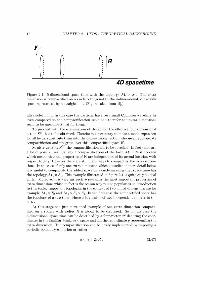
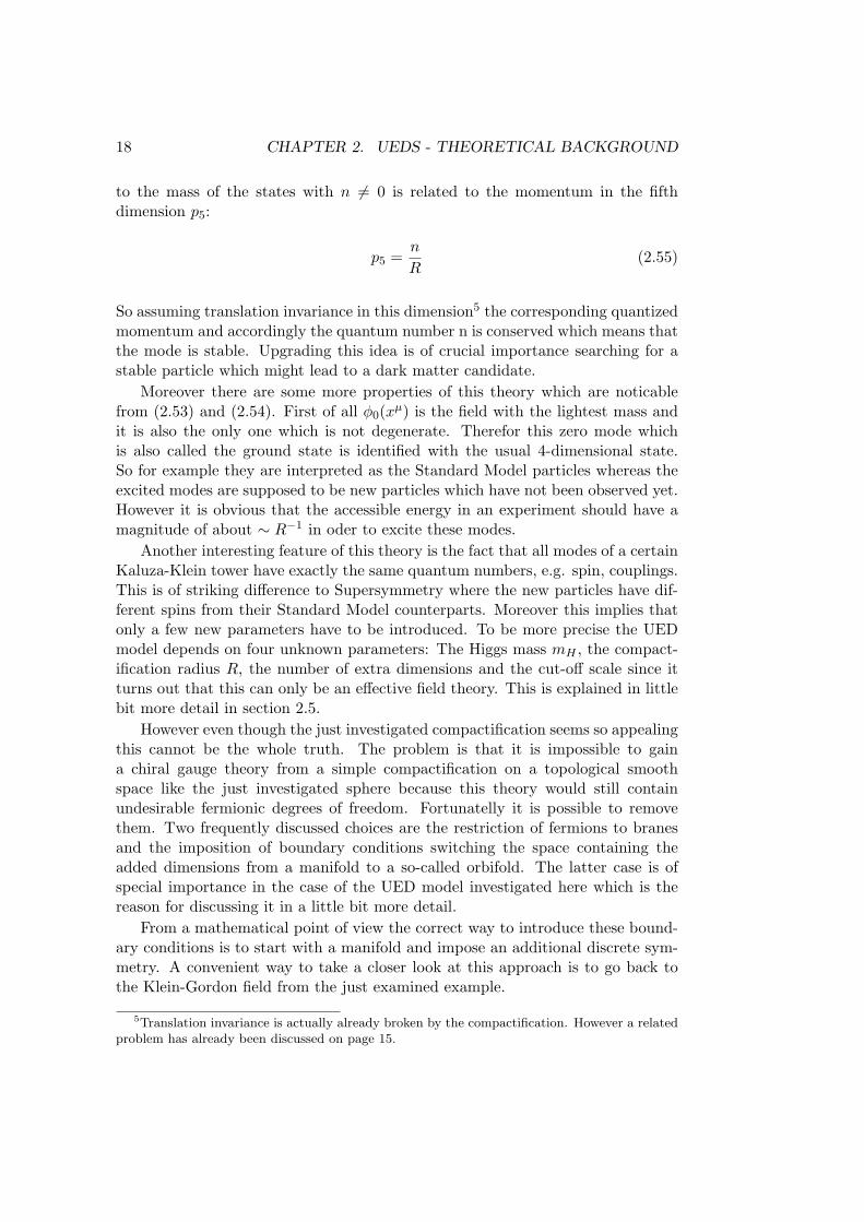
Figure 2.1: 5-dimensional space time with the topology M4 × S1. The extradimension is compactified on a circle orthogonal to the 4-dimensional Minkowskispace represented by a straight line. (Figure taken from [5].)
ultraviolet limit. In this case the particles have very small Compton wavelengthseven compared to the compactification scale and therefor the extra dimensionsseem to be uncompactified for them.
To proceed with the examination of the action the effective four dimensionalaction S(4) has to be obtained. Therefor it is necessary to make a mode expansionfor all fields, substitute them into the d-dimensional action, choose an appropriatecompactifiction and integrate over this compactified space K.
So after writting S(d) the compactification has to be specified. In fact there area lot of possibilities. Usually a compactification of the form M4 ×K is choosenwhich means that the properties of K are independent of its actual location withrespect toM4. However there are still many ways to compactify the extra dimen-sions. In the case of only one extra dimension which is studied in more detail belowit is useful to compactify the added space on a circle meaning that space time hasthe topologyM4 × S1. This example illustrated in figure 2.1 is quite easy to dealwith. Moreover it is very instructive revealing the most important properties ofextra dimensions which in fact is the reason why it is so popular as an introductionto this topic. Important topologies in the context of two added dimensions are forexampleM4 × T2 andM4 × S1 × S1. In the first case the compactified space hasthe topology of a two-torus whereas it consists of two independent spheres in thelatter.
At this stage the just mentioned example of one extra dimension compact-ified on a sphere with radius R is about to be discussed. So in this case the5-dimensional space time can be described by a four-vector xµ denoting the coor-dinates in the familiar Minkowski space and another coordinate y representing theextra dimension. The compactification can be easily implemented by imposing aperiodic boundary condition or rather
y ↔ y + 2πR . (2.47)
2.4. THE COMPACTIFICATION OF EXTRA DIMENSIONS 17
In order to discuss this kind of compactification a field has to be choosen which isabout to be examined. Obviously the easiest possibility is a complex scalar field Φobeying the Klein-Gordon equation in five dimensions
(∂K∂K +m2)Φ(xµ, y) = 0 (2.48)
with the Lagrangian
L =12
(∂KΦ(xµ, y)
)∗(∂KΦ(xµ, y)
)+
12m2∣∣∣Φ(xµ, y)
∣∣∣2 . (2.49)
Just as a reminder the capital Latin K runs from 0 to 4 as established on page 12.The 5-dimensional action is given by
S(5) =∫
dx4
∫ 2πR
0dy L . (2.50)
Incorporating the boundary condition (2.47) gives rise to the mode expansion
Φ(xµ, y) =1√2πR
∞∑n=−∞
φn(xµ)einyR . (2.51)
Inserting this expansion in the Lagrangain (2.49) and correspondingly (2.49) in(2.50) makes it very easy to evaluate the integration over the compactified dimen-sion. Using the well known orthogonality relation∫ 2πR
0dy e
i(n−m)yR = 2πδnm (2.52)
immediately yields the effective 4-dimensional action
S(4) =∫
dx4∞∑
n=−∞
[12
(∂νφn(xµ)
)∗(∂νφn(xµ)
)+
12
(m2 +n2
R2)∣∣∣φn(xµ)
∣∣∣2] .
(2.53)
Obviously the effective 4-dimensional theory describes nothing but an inifinitenumber often called Kaluza-Klein tower of Klein-Gordon fields φ(xµ) with themasses
m2n = m2 +
n2
R2. (2.54)
Taking a look at the expansion (2.51) it is evident that the additional contribution
18 CHAPTER 2. UEDS - THEORETICAL BACKGROUND
to the mass of the states with n 6= 0 is related to the momentum in the fifthdimension p5:
p5 =n
R(2.55)
So assuming translation invariance in this dimension5 the corresponding quantizedmomentum and accordingly the quantum number n is conserved which means thatthe mode is stable. Upgrading this idea is of crucial importance searching for astable particle which might lead to a dark matter candidate.
Moreover there are some more properties of this theory which are noticablefrom (2.53) and (2.54). First of all φ0(xµ) is the field with the lightest mass andit is also the only one which is not degenerate. Therefor this zero mode whichis also called the ground state is identified with the usual 4-dimensional state.So for example they are interpreted as the Standard Model particles whereas theexcited modes are supposed to be new particles which have not been observed yet.However it is obvious that the accessible energy in an experiment should have amagnitude of about ∼ R−1 in oder to excite these modes.
Another interesting feature of this theory is the fact that all modes of a certainKaluza-Klein tower have exactly the same quantum numbers, e.g. spin, couplings.This is of striking difference to Supersymmetry where the new particles have dif-ferent spins from their Standard Model counterparts. Moreover this implies thatonly a few new parameters have to be introduced. To be more precise the UEDmodel depends on four unknown parameters: The Higgs mass mH , the compact-ification radius R, the number of extra dimensions and the cut-off scale since itturns out that this can only be an effective field theory. This is explained in littlebit more detail in section 2.5.
However even though the just investigated compactification seems so appealingthis cannot be the whole truth. The problem is that it is impossible to gaina chiral gauge theory from a simple compactification on a topological smoothspace like the just investigated sphere because this theory would still containundesirable fermionic degrees of freedom. Fortunatelly it is possible to removethem. Two frequently discussed choices are the restriction of fermions to branesand the imposition of boundary conditions switching the space containing theadded dimensions from a manifold to a so-called orbifold. The latter case is ofspecial importance in the case of the UED model investigated here which is thereason for discussing it in a little bit more detail.
From a mathematical point of view the correct way to introduce these bound-ary conditions is to start with a manifold and impose an additional discrete sym-metry. A convenient way to take a closer look at this approach is to go back tothe Klein-Gordon field from the just examined example.
5Translation invariance is actually already broken by the compactification. However a relatedproblem has already been discussed on page 15.
2.4. THE COMPACTIFICATION OF EXTRA DIMENSIONS 19
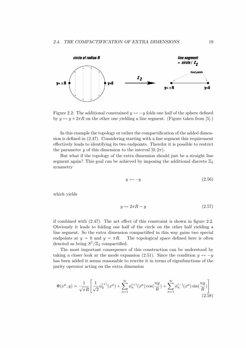
Figure 2.2: The additional constrained y ↔ −y folds one half of the sphere definedby y ↔ y+ 2πR on the other one yielding a line segment. (Figure taken from [5].)
In this example the topology or rather the compactification of the added dimen-sion is defined in (2.47). Considering starting with a line segment this requirementeffectively leads to identifying its two endpoints. Therefor it is possible to restrictthe parameter y of this dimension to the interval [0, 2π).
But what if the topology of the extra dimension should just be a straight linesegment again? This goal can be achieved by imposing the additional discrete Z2
symmetry
y ↔ −y (2.56)
which yields
y ↔ 2πR− y (2.57)
if combined with (2.47). The net effect of this constraint is shown in figure 2.2.Obviously it leads to folding one half of the circle on the other half yielding aline segment. So the extra dimension compactified in this way gains two specialendpoints at y = 0 and y = πR. The topological space defined here is oftendenoted as being S1/Z2 compactified.
The most important consequence of this construction can be understood bytaking a closer look at the mode expansion (2.51). Since the condition y ↔ −yhas been added it seems reasonable to rewrite it in terms of eigenfunctions of theparity operator acting on the extra dimension
Φ(xµ, y) =1√πR
[1√2φ
(+)0 (xµ) +
∞∑n=1
φ(+)n (xµ) cos(
ny
R) +
∞∑n=1
φ(−)n (xµ) sin(
ny
R)
](2.58)
20 CHAPTER 2. UEDS - THEORETICAL BACKGROUND
with the new functions φ(+)0 , φ(+)
n and φ(−)n being related to the formerly used
functions φn by
φ(+)0 = φ0 , φ(+)
n =1√2
(φn + φ−n) , φ(−)n =
i√2
(φn − φ−n) . (2.59)
As already stated this is just a rewriting of the former ansatz and therefor it isstill valid in the case of a compactification on a circle. However considering theadditional constraint (2.56) it is necessary to demand Φ to have a certain parityin order to obtain a good parity symmetry in the fifth dimension. Taking a lookat (2.58) achieving this goal is rather easy. If Φ is taken to be even all φ(−)
n mustvanish and accordingly if Φ is taken to be odd all φ(+)
n including φ(+)0 must vanish.
So the discrete symmetry (2.56) removes roughly half of the Kaluza-Klein modesand moreover also the degeneracy of the excited modes.6 So as already statedthis orbifold compactification makes it possible to obtain a chiral gauge theory byremoving unwanted fermionic degrees of freedom.
After all these abstract discussions it is necessary to take a look at the so-calledUED expansion of the Standard Model which is the topic of the next section.
2.5 Universal Extra Dimensions
Within the last few years three interesting models have been proposed which havedrawn quite some attention in the particle physics community. These are thealready mentioned ADD model submitted by Arkani-Hamad, Dimopoulos andDvali in 1998, the Randall-Sundrum model and Universal Extra Dimensions.
The first two ideas were mainly intended to address the hierarchy problem orrather the question why gravitation is so much weaker than the three StandardModelf interactions. Important properties of those models in contrast with Uni-versal Extra Dimensions are that the Randall-Sundrum model introduces warpedextra dimensions and in the ADD model only gravity is allowed to propagate inthe extra dimensions. In other words in the latter all forces except gravity arebound to the familiar four dimensional space called a brane in this context whereasgravity is admitted to the whole bulk.
After all this pre-banter the concept of Universal Extra Dimensions can beattacked. Great reviews on this topic are [6] and [7] with the later contrasting allthree introduced models. Apart from these review articles [8] and [9] have beenused for this chapter about the properties of Universal Extra Dimensions.
As expected this theory is distinguished by the fact that all Standard Modelparticles are promoted to the added extra dimensions.
6In fact the degeneracy is already broken by higher order mass corrections and therefor it isonly valid at tree level which will be shortly discussed in the next section.
2.5. UNIVERSAL EXTRA DIMENSIONS 21
At first sight this does not seem like a very appealing idea first of all becausefermions receive unwanted degrees of freedom using only a plain compactificationon a sphere. However as already addressed in section 2.4 this problem can beavoided by imposing an orbifold compactification. In order to understand whyit is impossible to gain a chiral gauge theory without additional constraints justconsider the projection operators used in the Standard Model to obtain left-handedand right-handed fermions
PL =1− γ5
2, PR =
1 + γ5
2(2.60)
leading to
ψL = PLψ , ψR = PRψ . (2.61)
Obviously the definition of γ5 is necessary. However for example in five dimensionsγ5 becomes a part of the group structure which can be seen by promoting theClifford algebra γµ, γµ = 2gµν to five dimensions with ΓA denoting the fivedimensional generalization of the Gamma matrices. An easy definition making thejust stated argument clear is Γµ = γµ and Γ4 = iγ5. So to sumarize this argumentit is not possible to define a matrix in five dimensions with the properties of γ5
in four dimensions which in turn makes it impossible to construct appropriateprojection operators.
So consider for example the S1/Z2 compactification already discussed before.The effective four dimensional Lagrangian of the Standard Model is easily derivedby writing down the five dimensional Lagrangian and integrating over the fifthdimension which in fact is the same approach used in section 5.3. The ratherlenghty result can be found for example in [6]. However it should be pointed outwhich kind of mode expansion is used for Standard Model fields. Considering theresult from the former section that wave functions are expected to have a certainparity with respect to the discrete Z2 symmetry the question arises which fieldsare supposed to be taken even and which ones odd. In the case of Gauge Bosonsand the Higgs Boson this choice is rather obvious. Since the zero modes whichcorrespond to the Standard model fields are removed from all odd fields it is clearthat all of these Standard Model particles have to be described by even wavefunctions. This gives rise to the expansions
Aµ(xµ, y) =1√πR
[1√2Aµ0 (xµ) +
∞∑n=1
Aµn(xµ) cos(ny
R)
]
A5(xµ, y) =1√πR
∞∑n=1
A5n(xµ) sin(
ny
R)
H(xµ, y) =1√πR
[1√2H0(xµ) +
∞∑n=1
Hn(xµ) cos(ny
R)
]. (2.62)
22 CHAPTER 2. UEDS - THEORETICAL BACKGROUND
As already mentioned this expansion is a little bit more tricky in the case offermions. However in this case the ansatz
ψ(xµ, y) =1√πR
[1√2ψ0(xµ)+
∞∑n=1
PLψL,n(xµ) cos(ny
R)+
∞∑n=1
PRψR,n(xµ) sin(ny
R)
](2.63)
is possible. In this formula ψ0 denotes the familiar Standard Model spinor chiralin four dimensions whereas ψL and ψR turn out to be vector-like in the effectivetheory. This rather complicated construction will not be explained here. Howeverit should be pointed out that the projection operators introduced here are thefamiliar four dimensional ones defined in (2.60).
At this stage a very important property of Universal Extra Dimensions shouldbe pointed out which is especially interesting in the context of dark matter. It isthe conservation of Kaluza-Klein parity. The basics have been already discussedin section 2.4. Nevertheless it is interesting to take a look at this property in moredetail.
First of all the UED model is the only theory introducing extra dimensionsgiving rise to a stable particle and hence to a viable dark matter candidate. Froma theoretical point of view this can be understood as follows:
Consider a theory assuming that some particles are allowed to propagate inthe bulk whereas other particles are trapped brane fields which means that theycannot leave the familiar four dimensional space time. Supposing that trappingparticles to the branes can be described by introducing Dirac δ-functions which isequal to neglecting the thickness of the brane the full five dimensional action S5
is given by
S(5) =∫
dx4
∫dy[Lbulk + Lbraneδ(y)
](2.64)
with the five dimensional Lagrangian Lbulk and the four dimensional Lbrane forthe particles traped on the brane. For example actions of this form are used in theADD model mentioned above. Of course, however there are no δ-functions presentin the action describing the UED model. This lacking of δ-functions has a veryimportant consequence for the kinds of Kaluza-Klein modes which are allowed toparticipate in an interaction.
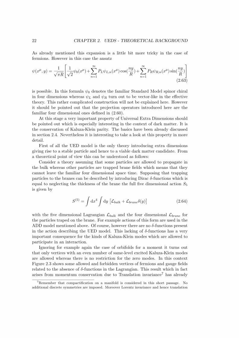
Ignoring for example again the case of orbifolds for a moment it turns outthat only vertices with an even number of same-level excited Kaluza-Klein modesare allowed whereas there is no restriction for the zero modes. In this contextFigure 2.3 shows some allowed and forbidden vertices of fermions and gauge fieldsrelated to the absence of δ-functions in the Lagrangian. This result which in factarises from momentum conservation due to Translation invariance7 has already
7Remember that compactification on a manifold is considered in this short passage. Noadditional discrete symmetries are imposed. Moreover Lorentz invariance and hence translation
2.5. UNIVERSAL EXTRA DIMENSIONS 23
Figure 2.3: A few allowed and forbidden vertices due to the absence of δ-functionsin the Lagrangian of the UED model which can arise in models incorporatingbranes. (Figure taken from [7].)
been obtained in section 4.6. To sum it up the Kaluza-Klein number is conservedwith respect to all interactions neglecting branes and orbifolds.
However as discussed before orbifolding is necessary to gain a more realisticmodel. Obviously this approach breaks translation invariance explicitely by intro-ducing for example two fixed points in the case of S1/Z2 which in fact is the onlyvalid compactification assuming one extra dimension.8 These fixed points giverise to localized interactions emerging via radiative corrections which turn out tobe of crucial importance in the case of Universal Extra Dimensions as describedlater in this section. Nevertheless a discrete subgroup called Kaluza-Klein paritydefined by PKK = (−1)n remains unbroken so that at least the lightest Kaluza-Klein mode is stable. It is this candidate which is specified below that gives riseto an important dark matter candidate.
Another implication which is not so significant considering direct detection ofdark matter but collider physics is the fact that all odd-level Kaluza-Klein modescan only be pair-produced. Anyway it should be pointed out that this breakingfrom Kaluza-Klein number conservation to Kaluza-Klein parity conservation isdue to radiative corrections which means that the former is still valid at treelevel and hence leads to loop-suppression of direct couplings to an even numberof Kaluza-Klein modes. Moreover it might be possible that renormalization givesrise to Kaluza-Klein parity breaking. However since this is rather unlikely andcannot be veryfied without having a full ultraviolet completion of the theory it isalways assumed that Kaluza-Klein parity is a good symmetry.
Another problem is the fact that the quantum field theory used to describethe Standard Model is not renormalizable in more than four dimensions. This canbe noticed by observing that the dimensions of the gauge couplings are negativein the case of added extra dimensions. This makes it necessary to introduce
invariance is supposed to be respected in the UV-limit or in other words by the short-lengthphysics as discussed on page 15.
8There are various possibilities considering six or more dimensions.
24 CHAPTER 2. UEDS - THEORETICAL BACKGROUND
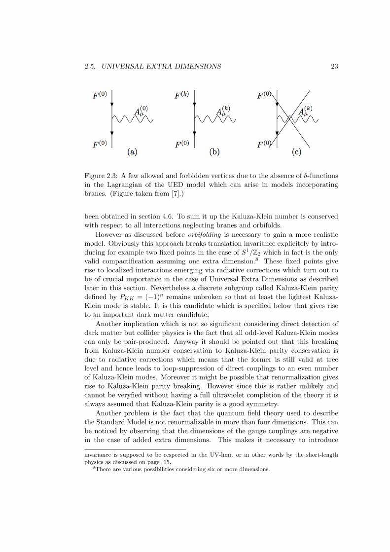
Figure 2.4: The mass spectrum of the level one Kaluza-Klein particles without(a) and with (b) considering first order radiative corrections. Asumed values areR−1 = 500 GeV, ΛR = 20 and mH = 120 GeV. (Figure taken from [9].)
another paramter except for the compactification radius R namely the cut-offscale Λ indicating that this is just an effective field theory. So all in all theUED model depends on four unknown parameters: The Higgs mass mH , thecompactification radius R, the number of extra dimensions and the cut-off scaleΛ. Some more information about this problem is given immediately in the contextof mass corrections.
This sections deals with the mass spectrum of the Kaluza-Klein modes. In thecase of promoting the Standard model to five dimensions the formula for massesof the excited modes given in (2.54) still holds at tree level:
m2n = m2 +
n2
R2(2.65)
(2.65) where m is again just the mass of the corresponding Standard model parti-cle suggests a high degree of degeneracy considering the low value of R discussedbelow. However it turns out that radiative corrections are really important con-sidering this UED model.
Radiative corrections are given rise to in two different ways. First of all thereare the already mentioned corrections localized on the fix points of the orbifold.Computing the corresponding contributions reveals that they all diverge logarith-mic with respect to the cut-off parameter Λ.
The second kind of radiative corrections is due to loop diagramms which areusually difficult to deal with especially in higher dimensional theories since in thiscase the Standard model is not supposed to be renormalizeable as already pointedout before. In this case though the loops include propagation in the compactifiedextra dimensions leading to an exponential suppression for momenta which arelarge in comparison to the scale of the extra dimension. Therefor the obtainedresults in this second case are finite.
2.5. UNIVERSAL EXTRA DIMENSIONS 25
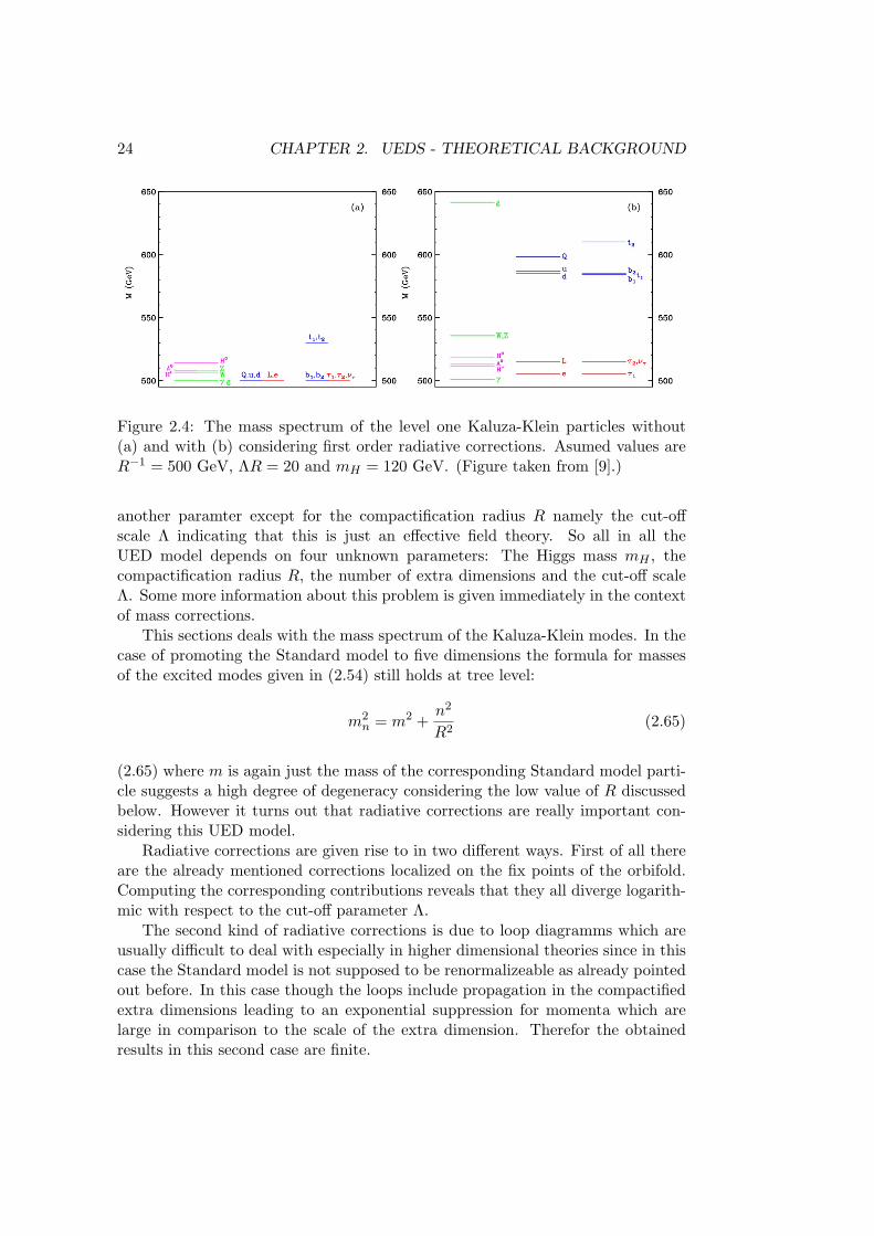
Figure 2.5: Dependence of the Weinberg angle for the first five Kaluza-Klein modesusing appropriate values for the parameters R and ΛR. In (a) the latter is fixedwhereas the former is fixed in (b). (Figure taken from [9].)
The complete spectrum of Kaluza-Klein particles has been computed and isgiven in [9]. Instead of quoting the results it is more instructive to take a look atfigure 2.4 which shows the spectrum without (a) and with (b) radiative correctionsof first order. Appropriate values given in the caption are explained hereafter. Asexpected neglecting all radiative corrections yields a quite degenerated spectrumwhich is broken by the incorporation of first order contributions. So higher orderterms change the spectrum in a way that will make its distinction from Super-symmetry models rather difficult. However it should be kept in mind that thiscomputation is based on some assumptions which do not necessarily need to betrue though they are quite suggesting. Without examining the details it should bementioned that the spectrum could possibly be quite different especially insofarthat the lightest Kaluza-Klein particle is not essentially the first excited mode ofthe photon. So even though an appropriate dark matter candidate could also begiven by the first Kaluza-Klein mode of a neutrino, the Higgs boson or even thegraviton this work has been focused on the photon since this is widely believed tobe the most probable candidate within the dark matter community. To underpinthis assumption it should be pointed out that gravitons would probably not anihi-late very effective due to the weakness of gravitational interactions and hence leadto an overclosure of the universe. Moreover consideration of the ν(1) has led to theresult that expected cross sections would probably be so high that they shouldhave already been detected. The corresponding computations are published in[10].
Finally consider the identification of the lightest Kaluza-Klein particle in moredetail. It is well known that electroweak symmetry-breaking mixes the bosonsB and W3 to gain the Z and the γ. The mixing is determined by the Weinbergangle θW given by sin2 θW = 0.23. Examining the corresponding matrix mix-
26 CHAPTER 2. UEDS - THEORETICAL BACKGROUND
ing the first level Kaluza-Klein modes and incorporating the first level radiativecorrections the result
(Z(1)
γ(1)
)=(
1R2 + 1
4g21v
2 + δM21
14g1g2v
2
14g1g2v
2 1R2 + 1
4g22v
2 + δM22
)(W
(1)3
B(1)
)(2.66)
with the U(1) and SU(2) gauge couplings g1 and g2 repectively, the Higgs vacuumexpectation value v ≈ 174 GeV and the radiative corrections δM2
1 and δM22 to
the B(1) and W (3) is obtained. Evaluating the already mentioned corrections givenin [9] reveals that the Weinberg angle for excited Kaluza-Klein modes is shiftedto quite small values for reasonable parameters as cognizable from figure 2.5.Therefor according to
γ(1) = B(1) cos θ(1)W +W
(1)3 sin θ(1)
W (2.67)
it is an appropriate approximation to consider γ(1) as being entirely B(1) in orderto simplify the upcoming computations.
Before proceeding with considerations of the B(1) as a dark matter candidatejust a few annotations about the magnitudes of the compactification radius R andthe cutoff scale Λ. An estimate on R is given in [8]. In this paper the authors dis-cuss their evaluation of electroweak precision observables and corrections relatedto one-loop contributions from Kaluza-Klein modes. They argue that constrainsrelated to these modes are rather weak because as already discussed there are noadditional contributions from the UED model at tree level. Finally they place anupper bound of
1R
& 300 GeV (2.68)
on the compactification radius considering one added extra dimension and a boundof
1R
& 400 to 800 GeV (2.69)
for two extra dimensions. The reason for giving an interval in the latter case isthe fact that the result is logarithmically divergent and therefor depends on thecutoff which is an unknown parameter as well. This problem does not occur forfive dimensions. So considering one extra dimension the bounds can be reliablycomputed in the framework of the effective theory whereas this is rather difficultassuming more extra dimensions. However it is obvious that the bounds seem to bein a range of a few hundred GeV which makes this theory testable at the Tevatronand the LHC. As already mentioned for example the ADD model includes trapping
2.5. UNIVERSAL EXTRA DIMENSIONS 27
some particles on the brane which leads to tree-level corrections to electroweakobservables in turn yielding upper bounds on R in the range of a few TeV. Itis especially this pleasant property and the occurance of a viable dark mattercandidate which drew a lot of attention to the UED model in recent years.
Considering the cutoff scale a simple estimate is given in [7]. There an upperbound on ΛR is estimated to be around 30 for five dimensions and about 10 forsix dimensions. Therefor in general the cutoff is estimate to have a magnitude ofabout
Λ ∼ 10R
. (2.70)
The last part of this section on the UED model deals with some properties of aviable dark matter candidate.
In order to really decide if a theory gives rise to a possible dark matter candi-date a stable particle is needed which in turn yields an appropriate value for thedark matter relic density of our universe ΩDM . So according to [11] it should bein the range of
0.095 < ΩDMh2 < 0.129 (2.71)
with the Hubble expansion rate given approximately by h = 0.71.As already discussed the particle of interest is the B(1) which is expected to be
in thermal equilibrium in the early universe and non-relativistic when it comes tothe freeze-out. In this case calculating the relic density of a particle is relativelyeasy if no coannihilation processes need to be considered. Assuming the validityof the just made assumptions it is justified to expect that the number density nof the B(1) which is its own antiparticle is governed by the Boltzmann equation
dndt
+ 3Hn = −〈σv〉(n2 − n2
eq
)(2.72)
with the Hubble paramter H, the relative velocity v, the annihilation cross sectionσ and the Boltzmann supressed number density neq in thermal equilibrium givenby
neq = g
(mT
2π
) 32
e−mT . (2.73)
Clearly m is the mass of the B(1), g the number of its internel degrees of freedomand T the temperature of the universe. Moreover it should be mentioned that〈. . .〉 in (2.72) denotes thermal averaging. As a reminder the freeze-out takesplace when the annihilation rate Γ = n〈σv〉 drops below the Hubble parameter H.
28 CHAPTER 2. UEDS - THEORETICAL BACKGROUND
However as pointed out and executed in [12] in the case of the UED model itis absolutely necessary to include coannihilation processes to obtain results thatare trustworthy. As already described in detail the mass spectrum is exceedinglydegenerate at tree level. However taking a look Figure 2.4 might give reason tothe assumption that coannihilation processes could be neglected because the de-generacy is broken by radiative corrections. Nevertheless it was already indicatedthat these corrections depend on assumptions about unknown physics at the cutoffscale so that these computations are not necessarily correct. Therefor in order tobe safe from possible mistakes it seems much more reliable to take coannihilationsinto account. Moreover it is obvious from Figure 2.4 that the degeneracy is notcompletely broken at least not for certain particles.
Thus the authors of [12] incorporated coannihilation processes with all otherfirst level Kaluza-Klein particles. This is accomplished by generalizing (2.72)taking the occurance of other particles into account. Consider an ensemble of Nnearly degenerated particles χi with masses mi and χ1 = B(1). Then it can beshown that the number density of the lightest of these particles is given by
dndt
+ 3Hn = −〈σeffv〉(n2 − n2
eq
). (2.74)
So σ in (2.74) has to be replaced by an effective cross section σeff which is givenby
σeff =N∑
i,j=1
σijgigjg2eff
(1 + ∆i)32 (1 + ∆j)
32 e−x(∆i−∆j) (2.75)
with
geff =N∑i=1
gi(1 + ∆i)32 e−x∆i (2.76)
and the degeneracy parameter
∆i =mi −m1
mi(2.77)
describing the fractional mass splitting between the particle χi and the B(1) whichis also of importance as a paramter in investigations described in chapters below.After solving the Boltzmann equation the relic density ρDM of the possible darkmatter candidate is easily obtained by ρDM = nm1 which in turn yields ΩDM
using
ΩDM =ρDMρc
(2.78)
2.5. UNIVERSAL EXTRA DIMENSIONS 29
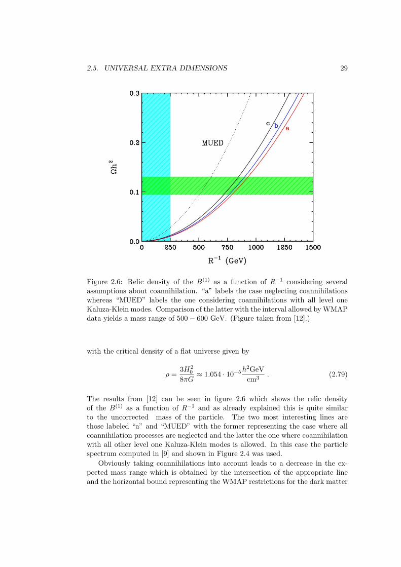
Figure 2.6: Relic density of the B(1) as a function of R−1 considering severalassumptions about coannihilation. “a” labels the case neglecting coannihilationswhereas “MUED” labels the one considering coannihilations with all level oneKaluza-Klein modes. Comparison of the latter with the interval allowed by WMAPdata yields a mass range of 500− 600 GeV. (Figure taken from [12].)
with the critical density of a flat universe given by
ρ =3H2
0
8πG≈ 1.054 · 10−5h
2GeVcm3
. (2.79)
The results from [12] can be seen in figure 2.6 which shows the relic densityof the B(1) as a function of R−1 and as already explained this is quite similarto the uncorrected mass of the particle. The two most interesting lines arethose labeled “a” and “MUED” with the former representing the case where allcoannihilation processes are neglected and the latter the one where coannihilationwith all other level one Kaluza-Klein modes is allowed. In this case the particlespectrum computed in [9] and shown in Figure 2.4 was used.
Obviously taking coannihilations into account leads to a decrease in the ex-pected mass range which is obtained by the intersection of the appropriate lineand the horizontal bound representing the WMAP restrictions for the dark matter
30 CHAPTER 2. UEDS - THEORETICAL BACKGROUND
density given in (2.71). So it is obvious that the B(1) with a mass in the range ofabout 500 - 600 Gev indeed provides a possible dark matter candidate. Lightermasses would lead to over-annihilating and hence to under-producing of the relicabundance of dark matter whereas heavier values would give rise to more darkmatter than observed. However it should be kept in mind that this result wasobtained assuming that only the B(1) contributes to dark matter whereas it ispossible and even very likely that the dark matter is generated by more than oneparticle. In this case the B(1) would be even lighter. Moreover there are alsoother possible mechanisms which could produce dark matter apart from the ther-mal production discussed here like gravitational entropy injection. However the500 - 600 Gev interval will be used as a benchmark here.
In a later chapter it will be shown that current experiments are just startingto probe this interesting mass range. So considering previous annotations it lookslike the UED model is about to be testable pretty soon using direct detectionexperiments like the one described here as well as colliders. Therefor and due tothe fact that the theory is quite aestethic and rather simple it is really justifiedthat it has drawn so much attention recently.
The following chapters will deal with considerations about the direct detectionof the B(1).
Chapter 3
Cross sections of the B(1) andnuclei
After this extensive discussion about general properties of the UED model thisand the following chapters are about to deal with considerations regarding directdetection with earth bound detectors like those used by the CDMS and XENON10collaboration.
Obviously one of the most important properties in this context is the crosssection of the WIMP candidate considered and the used target nuclei. Thereforthis chapter is devoted to theoretical predictions on these cross sections. Eventhough as already stated the focus is set on the B(1) as the dark matter candidatemost of the following methods are completely general and independent of the kindof WIMP and target nuclei.
Taking a closer look at the mentioned cross sections it is essential to have acertain idea about some basic nuclear physics. Great reviews especially focussingon direct dark matter detection are given in [13] and [14].
So first of all the question arises whether the cross sections are actually ex-pected to be high enough to be detectable. Without going into the details at thisstage the answer to this question is probably ”yes”. This can be understood byrealizing that the considered dark mattar candidate has to have a certain couplingto ordinary matter. Of course this interaction is expected to be quite small but notneglectable since otherwise there would not have occured enough annihilation inthe early universe and the abundance would have to significantly exceed the mea-sured value given for example in (2.71). To conclude it is a well known fact fromquantum field theory that certain Feynman diagramms contributing for exampleto pair annihilation are related to scattering amplitudes by the so-called crossingsymmetry. Therefor a non-vanishing pair annihilation cross section from dark mat-ter particles to quarks gives rise to a non-vanishing dark matter candidate-quarkscattering cross section. This simple argument is quite encouraging.
In order to attack the problem of cross sections three steps have to be accom-plished which all have their own subtlety.
31
32 CHAPTER 3. CROSS SECTIONS OF THE B(1) AND NUCLEI
First of all the corresponding Feynman amplitudes at the particle physics levelhave to be computed. Of course this means that a theoretically motivated La-grangian is available describing the interaction of the considered WIMP and thequarks and gluons which constitute the nucleons and hence the nuclei. Obtain-ing an effective four dimensional Lagrangian in the framework of UEDs has beendecribed extensively in the previous chapter. Even though the number of newlyintroduced parameters in this model is quite small compared for example to Su-persymmetry all of these models generally have large uncertainties which are infact of crucial importance to the predicions for expected event rates.
Moreover it should be mentioned that these considerations usually need toincorporate interactions with internal quark loops in the nuclei which means thatthe couplings to all quarks and gluons need to be taken into account.
Besides this step usually only deals with the zero-momentum transfer limit.Unfortunatelly this assumption is not sufficient which is one of the reasons forintroducing form factors later on.
The second step is about leaving the quark-gluon content of the nucleons be-hind. In order to obtain WIMP-nucleon cross sections the matrix elements of thequark and gluon operators sandwiched between nucleon states are needed. Theseso-called hadronic matrix elements can be provided by physicist investigating ap-propriate scattering processes.
As expected the next step deals with the upgrade from the nucleon to thenucleus level. The way this is done is similar to the former step sandwiching thenucleon operators obtained before between two nucleon states. This effectivelyyields a suppression of the cross sections incorporated by introducing a form factorwhich also takes care of finite momentum transfer as mentiond before.
The first two steps will be explained in this chapter whereas the third step isthe main subject of the next one.
An important simplification when dealing with the direct detection of darkmatter arises from the fact that these interactions happen in the non-relativisticlimit which is appropriate for halo velocities with a magnitude of about 10−3c.This limit is discussed in great detail in [15] where an effective WIMP-nucleon La-grangian is considered. So the first two steps of the just explained accomplishmentare studied. The authors argue that in the non-relativistic limit the interaction ofa WIMP and a nucleon can be effectively described by a Lagrangian of the form
Lint = 4χ†χ(fpη†pηp + fnη
†nηn
)+16√
2GFχ†~σ
2χ
(apη†p
~σ
2ηp + anη
†n
~σ
2ηn
)+O(
q
mp,W)
(3.1)
where χ denotes the WIMP spinor and ηn and ηp denote the two-component Weylspinors of the neutron and proton respectively. MoreoverGF = 1.16637 · 10−5GeV−2
refers to Fermi’s constant and mp to the proton mass. All in all the whole pro-cess can be parameterized using only five quantities namely the Wimp mass mW
33
and the spin-independent (SI) WIMP-nucleon couplings fp and fn and the spin-dependent (SD) WIMP-nucleon couplings ap and an. So obviously only a scalarand an axial-vector interaction remain whereas all other parts can either be ne-glected or rewritten and incorporated in one of the two forms just mentioned.1
This result is really remarkable considering that it has been derived usingonly very general assumptions like general Lorentz invariance of the interactionLagrangian. Especially it should be pointed out that no constraints were imposedconsidering the framework of the theory so for example (3.1) holds for the non-relativistic limit of UED and Supersymmetry models as well.
But in order to take a look at the cross sections relevant to the investigationsmade here it is more convenient to go back to the quark level. Of course for adiscussion of the UED model the interaction of the B(1) and the quarks has to beconsidered. The interaction Lagrangian for this example is given in [15], too:
Lint = −14
(βq + γq)B†µ1 B1µqq −
i
4αqB
†1µB1νε
0µνρqγργ5q (3.2)
with
αq = 2g21mB(1)
Y 2qL
m2
q(1)L
−m2B(1)
+Y 2qR
m2
q(1)R
−m2B(1)
(3.3)
βq = 2Eqg21
Y 2qL
m2
q(1)L
+m2B(1)
(m2
q(1)L
−m2B(1))2
+ Y 2qR
m2
q(1)R
+m2B(1)
(m2
q(1)R
−m2B(1))2
(3.4)
γq = g1mq
2m2H
(3.5)
In (3.3), (3.4) and (3.5) mq(1)L
and mq(1)R
denote the masses of the first Kaluza-Kleinmodes of the left- and right-chiral quarks and g1 the hypercharge coupling definedby
g1 =e
cos θW=√
4παcos θW
≈ 0.34537 (3.6)
where the Weinberg angle θW ≈ 28.741 and the Sommerfeld fine-structure con-stant α ≈ 1
137.036 is used. Moreover the Higgs mass is abreviated mH and mq
obviously represents the masses of the Standard model quarks and YqL and YqRtheir hypercharges distinguishing between right-handed and left-handed particles.In the used convention the hypercharge is given by
1Even though this result seems so appealing it should be kept in mind that a possible sup-pression of the four used couplings relative to other occuring couplings has been prohibited whichseems reasonable but is not completely secure.
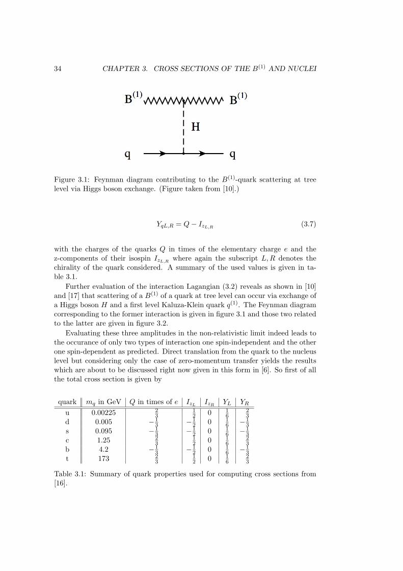
34 CHAPTER 3. CROSS SECTIONS OF THE B(1) AND NUCLEI
Figure 3.1: Feynman diagram contributing to the B(1)-quark scattering at treelevel via Higgs boson exchange. (Figure taken from [10].)
YqL,R = Q− IzL,R (3.7)
with the charges of the quarks Q in times of the elementary charge e and thez-components of their isospin IzL,R where again the subscript L,R denotes thechirality of the quark considered. A summary of the used values is given in ta-ble 3.1.
Further evaluation of the interaction Lagangian (3.2) reveals as shown in [10]and [17] that scattering of a B(1) of a quark at tree level can occur via exchange ofa Higgs boson H and a first level Kaluza-Klein quark q(1). The Feynman diagramcorresponding to the former interaction is given in figure 3.1 and those two relatedto the latter are given in figure 3.2.
Evaluating these three amplitudes in the non-relativistic limit indeed leads tothe occurance of only two types of interaction one spin-independent and the otherone spin-dependent as predicted. Direct translation from the quark to the nucleuslevel but considering only the case of zero-momentum transfer yields the resultswhich are about to be discussed right now given in this form in [6]. So first of allthe total cross section is given by
quark mq in GeV Q in times of e IzL IzR YL YR
u 0.00225 23
12 0 1
623
d 0.005 −13 −1
2 0 16 −1
3s 0.095 −1
3 −12 0 1
6 −13
c 1.25 23
12 0 1
623
b 4.2 −13 −1
2 0 16 −1
3t 173 2
312 0 1
623
Table 3.1: Summary of quark properties used for computing cross sections from[16].
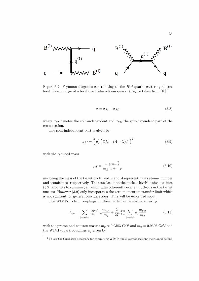
35
Figure 3.2: Feynman diagrams contributing to the B(1)-quark scattering at treelevel via exchange of a level one Kaluza-Klein quark. (Figure taken from [10].)
σ = σSI + σSD (3.8)
where σSI denotes the spin-independent and σSD the spin-dependent part of thecross section.
The spin-independent part is given by
σSI =4πµ2T
(Zfp + (A− Z)fn
)2(3.9)
with the reduced mass
µT =mB(1)m2
T
mB(1) +mT(3.10)
mT being the mass of the target nuclei and Z and A representing its atomic numberand atomic mass respectively. The translation to the nucleus level2 is obvious since(3.9) amounts to summing all amplitudes coherently over all nucleons in the targetnucleus. However (3.9) only incorporates the zero-momentum transfer limit whichis not sufficent for general considerations. This will be explained soon.
The WIMP-nucleon couplings on their parts can be evaluated using
fp,n =∑
q=u,d,s
f(p,n)Tq
aqmp,n
mq+
227fp,nTG
∑q=c,b,t
aqmp,n
mq(3.11)
with the proton and neutron masses mp ≈ 0.9383 GeV and mn = 0.9396 GeV andthe WIMP-quark couplings aq given by
2This is the third step necessary for computing WIMP-nucleus cross sections mentioned before.
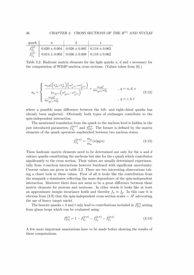
36 CHAPTER 3. CROSS SECTIONS OF THE B(1) AND NUCLEI
quark u d s
f(p)Tq
0.020± 0.004 0.026± 0.005 0.118± 0.062
f(n)Tq
0.014± 0.003 0.036± 0.008 0.118± 0.062
Table 3.2: Hadronic matrix elements for the light quarks u, d and s necessary forthe computation of WIMP-nucleon cross sections. (Values taken from [6].)
aq =
mqg21
(Y 2qR+Y 2
qL
)(m2
q(1)+m2
B(1)
)4m
B(1)
(m2
B(1)−m2
q(1)
)2 + mqg218m
B(1)m2H
, q = u, d, s
mqg218m
B(1)m2H
, q = c, b, t
(3.12)
where a possible mass difference between the left- and right-chiral quarks hasalready been neglected. Obviously both types of exchanges contribute to thespin-independent interaction.
The mentioned translation from the quark to the nucleon level is hidden in thejust introduced parameters f (p,n)
Tqand fp,nTG. The former is defined by the matrix
elements of the quark operators sandwiched between two nucleon states.
f(p,n)Tq
=mq
mn〈n|qq|n〉 (3.13)
These hadronic matrix elements need to be determined not only for the u and dvalence quarks constituting the nucleons but also for the s quark which contributessignificantly to the cross section. Their values are usually determined experimen-tally from π-nucleon interactions however burdened with significant uncertainty.Current values are given in table 3.2. There are two interesting observations tak-ing a closer look at these values. First of all it looks like the contribution fromthe seaquark s dominates reflecting the mass dependence of the spin-independentinteraction. Moreover there does not seem to be a great difference between thesematrix elements for protons and neutrons. In other words it looks like at leastan approximate isospin invariance holds and therefor fn ≈ fp. In this case it isobvious from (3.9) that the spin-independent cross section scales ∼ A2 advocatingthe use of heavy target nuclei.
The heavier quarks c, b and t only lead to contributions included in fp,nTG arisingfrom gluon loops which can be evaluated using
fp,nTG = 1− f (p,n)Tu
− f (p,n)Td
− f (p,n)Ts
(3.14)
A few more important annotations have to be made before showing the results ofthese computations.
37
First of all an assumption about the masses of the level one Kaluza-Kleinquarks has to be made since their values are at most vaguely known. It is acommon procedure to assume a quite high degree of degeneracy of these quarkmodes and introduce the so-called degeneracy parameter ∆
∆ =mq(1) −mB(1)
mB(1)
(3.15)
to impose a relation between these assumed to be totally degenerate level onequark masses and the mass of the B(1).
In fact this parameter and the Higgs mass mH are considered as additional pa-rameters apart from the WIMP mass mB(1) evaluating the spin-independent crosssection σSI . They enter the computation in (3.12) determining the WIMP-quarkcoupling. Obviously the occurance of a factor (m2
B(1) −m2q(1)
)2 in the denomina-tor in (3.12) considering the light quarks leads to a striking enhancement of theWIMP-quark coupling in the case that ∆ is extremly small. Such a degeneracy isusually not well motivated but it might be possible especially considering theorieslike the UED model where a general high degree of degeneracy occurs naturally.In the computations executed here ∆ is varied inside an interval from 0.01 to0.5 which seems quite reasonable taking the high degeneracy of the model intoaccount but omiting unexpected resonances. The other mentioned parameter theHiggs boson mass is varied from 114.4 to 200 GeV.
Moreover it is a useful procedure to normalize the cross sections obtained from(3.9) σSI to cross sections on a nucleon σp,nSI . This is of special importance consid-ering comparisons between different target nuclei. So evaluating (3.9) assumingthat the target solely consists of a proton or a neutron yields
σp,nSI =4πµp,nf
2p,n (3.16)
with
µp,n =mB(1)mp,n
mB(1) +mp,n. (3.17)
Comparing this result to the original expression (3.9) directly yields the relation
σp,nSI =f2p,n(
Zfp + (A− Z)fn)2
µ2p,n
µ2T
σSI (3.18)
which reduces to
σp,nSI =1A2
µ2p,n
µ2T
σSI (3.19)
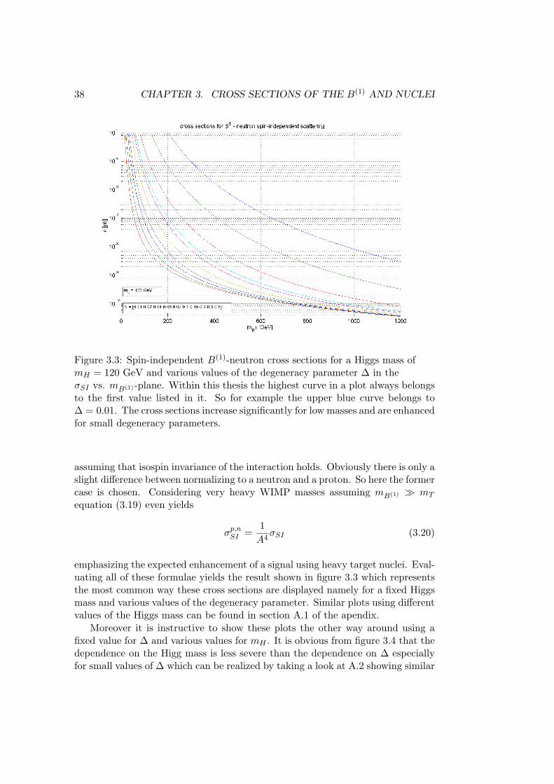
38 CHAPTER 3. CROSS SECTIONS OF THE B(1) AND NUCLEI
Figure 3.3: Spin-independent B(1)-neutron cross sections for a Higgs mass ofmH = 120 GeV and various values of the degeneracy parameter ∆ in theσSI vs. mB(1)-plane. Within this thesis the highest curve in a plot always belongsto the first value listed in it. So for example the upper blue curve belongs to∆ = 0.01. The cross sections increase significantly for low masses and are enhancedfor small degeneracy parameters.
assuming that isospin invariance of the interaction holds. Obviously there is only aslight difference between normalizing to a neutron and a proton. So here the formercase is chosen. Considering very heavy WIMP masses assuming mB(1) mT
equation (3.19) even yields
σp,nSI =1A4σSI (3.20)
emphasizing the expected enhancement of a signal using heavy target nuclei. Eval-uating all of these formulae yields the result shown in figure 3.3 which representsthe most common way these cross sections are displayed namely for a fixed Higgsmass and various values of the degeneracy parameter. Similar plots using differentvalues of the Higgs mass can be found in section A.1 of the apendix.
Moreover it is instructive to show these plots the other way around using afixed value for ∆ and various values for mH . It is obvious from figure 3.4 that thedependence on the Higg mass is less severe than the dependence on ∆ especiallyfor small values of ∆ which can be realized by taking a look at A.2 showing similar
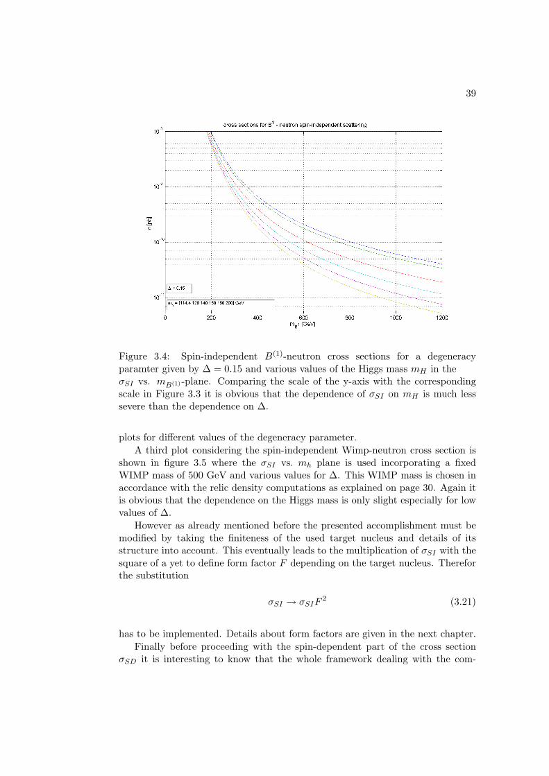
39
Figure 3.4: Spin-independent B(1)-neutron cross sections for a degeneracyparamter given by ∆ = 0.15 and various values of the Higgs mass mH in theσSI vs. mB(1)-plane. Comparing the scale of the y-axis with the correspondingscale in Figure 3.3 it is obvious that the dependence of σSI on mH is much lesssevere than the dependence on ∆.
plots for different values of the degeneracy parameter.A third plot considering the spin-independent Wimp-neutron cross section is
shown in figure 3.5 where the σSI vs. mh plane is used incorporating a fixedWIMP mass of 500 GeV and various values for ∆. This WIMP mass is chosen inaccordance with the relic density computations as explained on page 30. Again itis obvious that the dependence on the Higgs mass is only slight especially for lowvalues of ∆.
However as already mentioned before the presented accomplishment must bemodified by taking the finiteness of the used target nucleus and details of itsstructure into account. This eventually leads to the multiplication of σSI with thesquare of a yet to define form factor F depending on the target nucleus. Thereforthe substitution
σSI → σSIF2 (3.21)
has to be implemented. Details about form factors are given in the next chapter.Finally before proceeding with the spin-dependent part of the cross section
σSD it is interesting to know that the whole framework dealing with the com-
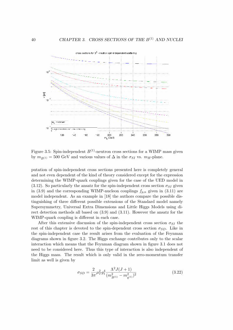
40 CHAPTER 3. CROSS SECTIONS OF THE B(1) AND NUCLEI
Figure 3.5: Spin-independent B(1)-neutron cross sections for a WIMP mass givenby mB(1) = 500 GeV and various values of ∆ in the σSI vs. mH -plane.
putation of spin-independent cross sections presented here is completely generaland not even dependent of the kind of theory considered except for the expressiondetermining the WIMP-quark couplings given for the case of the UED model in(3.12). So particularly the ansatz for the spin-independent cross section σSI givenin (3.9) and the corresponding WIMP-nucleon couplings fp,n given in (3.11) aremodel independent. As an example in [18] the authors compare the possible dis-tinguishing of three different possible extensions of the Standard model namelySupersymmetry, Universal Extra Dimensions and Little Higgs Models using di-rect detection methods all based on (3.9) and (3.11). However the ansatz for theWIMP-quark coupling is different in each case.
After this extensive discussion of the spin-independent cross section σSI therest of this chapter is devoted to the spin-dependent cross section σSD. Like inthe spin-independent case the result arises from the evaluation of the Feynmandiagrams shown in figure 3.2. The Higgs exchange contributes only to the scalarinteraction which means that the Feynman diagram shown in figure 3.1 does notneed to be considered here. Thus this type of interaction is also independent ofthe Higgs mass. The result which is only valid in the zero-momentum transferlimit as well is given by
σSD =2
3πµ2T g
41
Λ2J(J + 1)(m2
B(1) −m2q(1)
)2(3.22)
41
with
Λ =ap〈Sp〉+ an〈Sn〉
J(3.23)
where J denotes the total nuclear spin and 〈Sp,n〉 the expectation values of theproton and neutron spins within the nucleus. Since these last quantities have tobe computed using nuclear structure calculations which is usually accomplishedin connection with the analysis of form factors a discussions of these quantities isdeferred to the next chapter. ap and an are the WIMP-proton and WIMP-neutroncouplings respectively containing details of the UED model and the quark spincontent ot the nucleons.
What makes the investigation of spin-dependent cross sections comparativelydifficult is the fact that in this case the WIMP does not just couple to the numberof nucleons in the nucleus but to their spins. So even though the interactionwith the nucleus is coherent as in the spin-independent case in the sense that thescattering amplitudes are still summed the strength of the interaction vanishes forpaired nucleons in the same energy state since the sign of the interaction amplitudeswitches together with the nucleon spin. If their energy states are different theeffective interaction rate is highly suppressed but still finite. Nevertheless thismeans that only nuclei with an odd number of nucleons yield a significant crosssection and that other nuclei can be neglected. The WIMP-nucleon couplings aregiven by
ap,n =∑
q=u,d,s
(Y 2qL + Y 2
qR)∆p,nq (3.24)
where the parameters ∆p,nq represent the translation from the quark to the nu-cleon level. An important difference to the spin-independent case is that thesecouplings are generally not even approximately equal and that they may evenvary by several orders of magnitude. Similar to the quantities f (p,n)
Tqdefined in
(3.13) the ∆p,nq’s are given by the matrix element of the quark axial-vector currentor rather
sp,nµ ∆p,nq =12〈n|qγµγ5q|n〉 (3.25)
with the nucleon spin sp,nµ . Obviously the quantity ∆p,nq parameterizes the contri-bution of each quark q to the total spin of the nucleon n. The corresponding val-ues are experimentally determined from investigations of polarized lepton-nucleondeep inelastic scattering. Current values are given in table 3.3. Especially compar-ing the errors of these values to those for the parameters f (p,n)
Tqgiven in table 3.2
shows that they cannot be measured to a great precision and hence that they area large source of uncertainty in the calculations.
42 CHAPTER 3. CROSS SECTIONS OF THE B(1) AND NUCLEI
Inserting the values from Table 3.3 and the hypercharges given in Table 3.1into (3.24) yields
ap = 0.281an = −0.139 . (3.26)
Obviously the WIMP-nucleon couplings in the spin-dependent case are indepen-dent of the model parameters ∆ and mH which is totally different from the spin-independent case cp. (3.11) with (3.12). However the expression (3.22) for thespin-dependent cross section σSD is directly dependent on ∆ via the mass of thelevel one Kaluza-Klein quarks. Therefor it is clear that this formula is modeldependet. This should be contrasted to the spin-independent case where it waspointed out that the expression (3.9) yielding σSI is model independent and forexample valid in the case of an UED and supersymmetric model as well.
However the normalization to a nucleon analogue to (3.20) is again modelindependent. To accomplish this normalization (3.22) has to be evaluated for asingle nucleon. In this case J = 1
2 holds and the nucleon spin expectation valuesare given by 〈Sp〉 = 1
2 and 〈Sn〉 = 0 whether a proton is considered or by 〈Sp〉 = 0and 〈Sn〉 = 1
2 in the case of a neutron. Using these values directly yields
σp,nSD =1
2πg4
1
µ2p,na
2p,n
(m2B(1) −m2
q(1))2
. (3.27)
Comparing this result to (3.22) gives rise to the normalization
σp,nSD =34µ2p,n
µ2T
J
J + 11
〈Sp,n〉2σSD (3.28)
which is analogue to (3.19) and as already mentioned model independent as well.However as already mentioned another important difference to the spin-independent
case can be realized by evaluating (3.27) for a proton and a neutron which is shownin figure 3.6 and figure 3.7 respectively: Obviously there is a large difference be-tween both cases which in fact is not really surprising since the WIMP-proton andWIMP-neutron couplings given in (3.26) differ a lot. This should be contrasted
quark u d s∆pq 0.78± 0.02 −0.48± 0.02 −0.15± 0.07∆nq −0.48± 0.02 0.78± 0.02 −0.15± 0.07
Table 3.3: Matrix elements of the quark axial-vector current for the light quarksu, d and s necessary for the computation of WIMP-nucleon cross sections. Thevalues corresponding to the proton and neutron are connected by flavor isospinrotation. (Values taken from [6].)
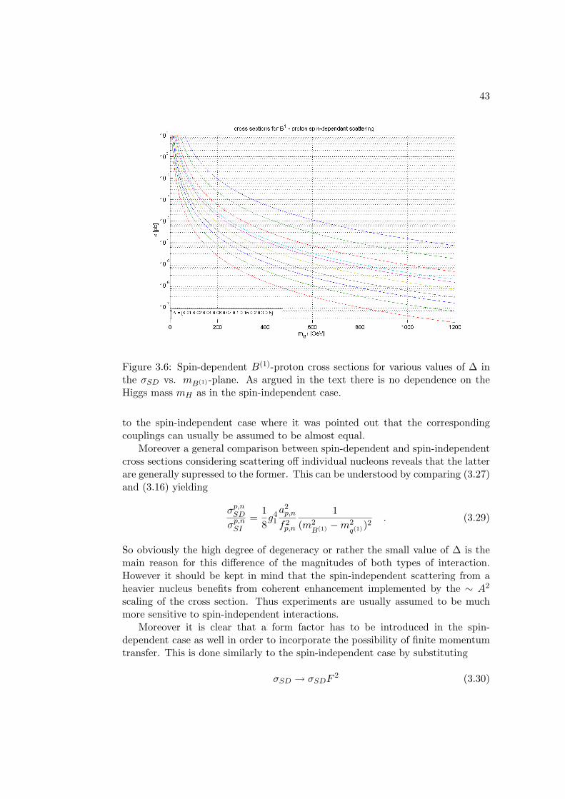
43
Figure 3.6: Spin-dependent B(1)-proton cross sections for various values of ∆ inthe σSD vs. mB(1)-plane. As argued in the text there is no dependence on theHiggs mass mH as in the spin-independent case.
to the spin-independent case where it was pointed out that the correspondingcouplings can usually be assumed to be almost equal.
Moreover a general comparison between spin-dependent and spin-independentcross sections considering scattering off individual nucleons reveals that the latterare generally supressed to the former. This can be understood by comparing (3.27)and (3.16) yielding
σp,nSDσp,nSI
=18g4
1
a2p,n
f2p,n
1(m2
B(1) −m2q(1)
)2. (3.29)
So obviously the high degree of degeneracy or rather the small value of ∆ is themain reason for this difference of the magnitudes of both types of interaction.However it should be kept in mind that the spin-independent scattering from aheavier nucleus benefits from coherent enhancement implemented by the ∼ A2
scaling of the cross section. Thus experiments are usually assumed to be muchmore sensitive to spin-independent interactions.
Moreover it is clear that a form factor has to be introduced in the spin-dependent case as well in order to incorporate the possibility of finite momentumtransfer. This is done similarly to the spin-independent case by substituting
σSD → σSDF2 (3.30)
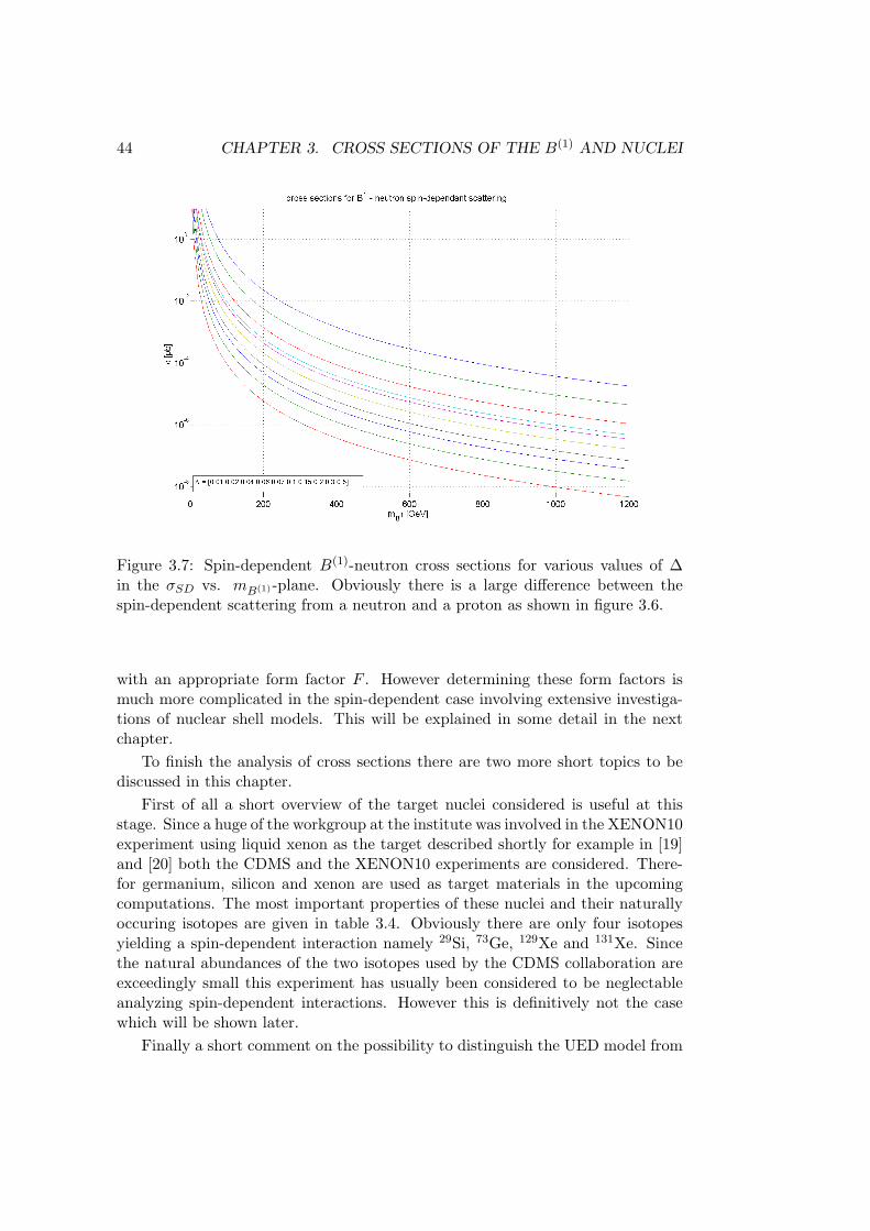
44 CHAPTER 3. CROSS SECTIONS OF THE B(1) AND NUCLEI
Figure 3.7: Spin-dependent B(1)-neutron cross sections for various values of ∆in the σSD vs. mB(1)-plane. Obviously there is a large difference between thespin-dependent scattering from a neutron and a proton as shown in figure 3.6.
with an appropriate form factor F . However determining these form factors ismuch more complicated in the spin-dependent case involving extensive investiga-tions of nuclear shell models. This will be explained in some detail in the nextchapter.
To finish the analysis of cross sections there are two more short topics to bediscussed in this chapter.
First of all a short overview of the target nuclei considered is useful at thisstage. Since a huge of the workgroup at the institute was involved in the XENON10experiment using liquid xenon as the target described shortly for example in [19]and [20] both the CDMS and the XENON10 experiments are considered. There-for germanium, silicon and xenon are used as target materials in the upcomingcomputations. The most important properties of these nuclei and their naturallyoccuring isotopes are given in table 3.4. Obviously there are only four isotopesyielding a spin-dependent interaction namely 29Si, 73Ge, 129Xe and 131Xe. Sincethe natural abundances of the two isotopes used by the CDMS collaboration areexceedingly small this experiment has usually been considered to be neglectableanalyzing spin-dependent interactions. However this is definitively not the casewhich will be shown later.
Finally a short comment on the possibility to distinguish the UED model from
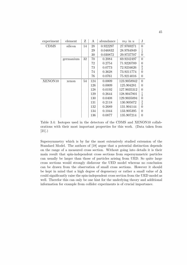
45
experiment element Z A abundance mT in u JCDMS silicon 14 28 0.922297 27.9769271 0
29 0.046832 28.9764949 12
30 0.030872 29.9737707 0germanium 32 70 0.2084 69.9242497 0
72 0.2754 71.9220789 073 0.0773 72.9234626 9
274 0.3628 73.9211774 076 0.0761 75.9214016 0
XENON10 xenon 54 124 0.0009 123.9058942 0126 0.0009 125.904281 0128 0.0192 127.9035312 0129 0.2644 128.9047801 1
2130 0.0408 129.9035094 0131 0.2118 130.905072 3
2132 0.2689 131.904144 0134 0.1044 133.905395 0136 0.0877 135.907214 0
Table 3.4: Isotopes used in the detectors of the CDMS and XENON10 collab-orations with their most important properties for this work. (Data taken from[21].)
Supersymmetry which is by far the most extensively studied extension of theStandard Model. The authors of [18] argue that a potential distinction dependson the range of a measured cross section. Without going into details it is theirmain result that spin-independent cross sections from supersymmetric particlescan usually be larger than those of particles arising from UED. So quite largecross sections would strongly disfavour the UED model whereas no conclusioncan be drawn from the observation of small cross sections. However it shouldbe kept in mind that a high degree of degeneracy or rather a small value of ∆could significantly raise the spin-independent cross section from the UED model aswell. Therefor this can only be one hint for the underlying theory and additionalinformation for example from collider experiments is of crucial importance.
Chapter 4
Form factors
As described in the previous chapter it is necessary to introduce form factors tomodify the cross sections in order to incorporate non-zero momentum transferwhich is inevitable considering heavy WIMPs of a few 10’s of GeV or more. Tobe more precise the structure of the nucleon has to be taken into account whenthe momentum transfer q given by
q =√
2mTER (4.1)
with the recoil energy ER yields a corresponding de Broglie wave length λ = hq
which is no longer large compared to the effective nuclear radius rn. These formfactors should be normalized to 1 for zero momentum transfer and smaller than1 otherwise. Great reviews dealing with form factors and related nuclear shellmodel calculations necessary in the spin-dependent case are given in [13], [22] and[23].
Without going into the details of the underlying nuclear physics it can beshown that both kinds of form factors can be written in a similar form ensuringthe normalization constraint namely
F 2SI(q) =
SSI(q)SSI(0)
and F 2SD(q) =
SSD(q)SSD(0)
(4.2)
with
SSI(q) =∑L even
|〈J ||CL(q)||J〉|2 ' |〈J ||C0(q)||J〉|2 (4.3)
and
SSD(q) =∑L odd
(|〈J ||T el5L (q)||J〉|2 + |〈J ||L5
L(q)||J〉|2)
(4.4)
46
4.1. SPIN-INDEPENDENT FORM FACTORS 47
where the double vertical lines denote the reduced matrix elements of the respec-tive operators. In (4.4) T el5L and L5
L denote the transverse electric and longitudinalmultipole projections of the axial vector current respectively. CL in (4.3) repre-sents the so-called coulomb projection. The explicit forms of these operators canbe found in any of the just mentioned review articles. The simplification in (4.3)is justified because the contribution from L = 0 dominates so that the rest can beneglected.
Since the form given in (4.2) will not be needed in the spin-independent casethe subscript of S will be dropped in the following considerations. Therefor Salways denotes the spin-dependent case from now on.
The following two sections deal with both types of form factors seperatelystarting with the much simpler spin-independent case.
4.1 Spin-independent form factors
As mentioned before the spin-independent case is rather easy to treat since thenthe WIMPs couple only to the number of nucleons in the nucleus. A short intro-duction to this topic can be found in [24].
So considering the first Born approximation the form factor FSI is just givenby the Fourier transformation of the mass density distribution ρ which in turnis usually assumed to be proportional to the charge density distribution. This isnecessary because the latter is known to a much higher accuracy from low-energyelastic lepton scattering which in turn is observed to be isotropic justifying theansatz ρ(~r) = ρ(r) yielding FSI(~q) = FSI(q). So FSI can be computed using
FSI(q) =∫ρ(r)ei~q·~rd3r =
4πq
∫ ∞0
r sin(qr)ρ(r)dr . (4.5)
A lot of different density distributions have been proposed in the literature. Ac-cording to [24] the most realistic one is the Fermi distribution given by
ρ(r) = ρ01
1 + er−ca
. (4.6)
However a proposal originally made by Helm in [25] half a century ago is usuallypreferred because its Fourier transformation can be evaluated analytically whereasthe ansatz (4.6) demands numerical evaluation of (4.5). Moreover it turns outthat both forms yield quite similar results. Helm considered a folded densitydistribution of the form
ρ(~r) =∫ρ0(~r′) ρ1(~r − ~r′)d3r′ . (4.7)
Observing that the scattering depends mainly on the charge distribution near the
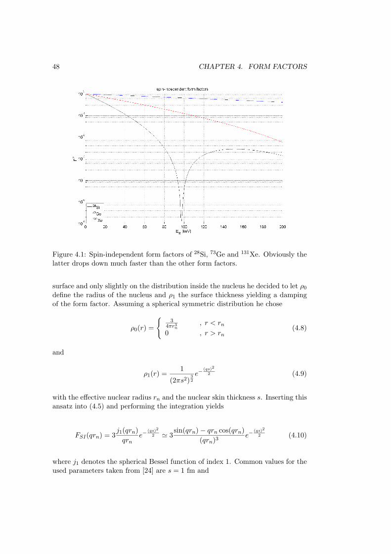
48 CHAPTER 4. FORM FACTORS
Figure 4.1: Spin-independent form factors of 28Si, 73Ge and 131Xe. Obviously thelatter drops down much faster than the other form factors.
surface and only slightly on the distribution inside the nucleus he decided to let ρ0
define the radius of the nucleus and ρ1 the surface thickness yielding a dampingof the form factor. Assuming a spherical symmetric distribution he chose
ρ0(r) =
3
4πr3n, r < rn
0 , r > rn(4.8)
and
ρ1(r) =1
(2πs2)32
e−(qs)2
2 (4.9)
with the effective nuclear radius rn and the nuclear skin thickness s. Inserting thisansatz into (4.5) and performing the integration yields
FSI(qrn) = 3j1(qrn)qrn
e−(qs)2
2 ' 3sin(qrn)− qrn cos(qrn)
(qrn)3e−
(qs)2
2 (4.10)
where j1 denotes the spherical Bessel function of index 1. Common values for theused parameters taken from [24] are s = 1 fm and
4.2. SPIN-DEPENDENT FORM FACTORS 49
rn =
√c2 +
73π2a2 − 5s2 (4.11)
with a = 0.52 fm and
c = 1.23 3√A− 0.60 fm . (4.12)
The just explained analysis highlights an important difference from the spin-dependent case considered in the next section: The spin-independent form factorsFSI are almost independent of the used target nuclei except for the values of theiratomic masses A. In particular there is no dependence on the spin-independentWIMP-nucleon couplings fp and fn which turns out to be a great benefit deter-mining cross section limits.
Finally figure 4.1 shows a comparison of spin-independent form factors for onesilicon, one germanium and one xenon isotope. Obviously the form factor fromthe xenon isotope drops down much faster than the form factors from the siliconand the germanium isotopes partly compensating the xenon benefit from the ∼ A2
scaling. However considering really low thresholds the use of xenon seems to bemore advantageous.
4.2 Spin-dependent form factors
Computing form factors in the spin-dependent case is considerably more compli-cated because the spin structure varies enormously between different target nuclei.Therefor they have to be computed separately for every single target isotope usingextensive nuclear shell model calculations.
Considering zero momentum transfer (4.4) can be evaluated explicitely sincemost contributions to the sum vanish. The result is given by
S(0) =2J + 1π
J(J + 1)Λ2 (4.13)
with Λ given in (3.23). Obviously knowledge of the expectation values of theproton and neutron spins within the nucleus 〈Sp〉 and 〈Sn〉 as well as of the WIMPnucleon couplings ap and an is necessary.
At finite momentum transfer it is inevitable to consider more complicated ap-proaches. The applied formalism is in fact a generalization of the one accomplishedfor the investigation of weak and electromagnetic semi-leptonic interactions in nu-clei. It is a common procedure to switch from the proton-neutron representationto the isospin representation. This is implemented by writing the isoscalar and
50 CHAPTER 4. FORM FACTORS
isovector spin couplings a0 and a1 in terms of the WIMP-proton and WIMP-neutron couplings ap and an.
a0 = ap + an
a1 = ap − an . (4.14)
Using this translation (4.4) can be written in the form
S(q) = a20S00(q) + a2
1S11(q) + a0a1S01(q) (4.15)
with the spin structure functions S00, S11 and S01 representing an isoscalar, isovec-tor and interference term respectively.
Considering the dependence of the WIMP-nucleon couplings it can be seenthat the form of S(q) is determined solely by the ratio ap
anwhereas its magnitude
is proportional to a2p+a2
n. Since according to (4.2) the squared form factor is givenby (4.15) normalized to 1 for q = 0 it is clear that F 2 is solely determined by theratio ap
an. Knowledge of the absolute value of neither one of the WIMP-nucleon
couplings is required.Moreover it should already be noted at this stage that evaluating (4.15) at
q = 0 can be very problematic since S(0) can reach 0 for certain values of apan leadingto a singularity in the expression (4.2) for F 2. Fortunately there is no problemusing the WIMP-nucleon couplings from the UED model given in (3.26). Howeverthis problem occurs determining limits on WIMP-nucleon couplings as explained ina later chapter. It can partly be solved by using (4.13) in the denominator of (4.2)instead of evaluating (4.15) at q = 0. It should be kept in mind that in practicethis substitution leads to a slight violation of the normalization constraint sinceevaluating (4.15) using fitted functions as explained below only approximatelyyields (4.13). Anyway this accomplishment makes it possible to avoid singularities.Nevertheless other difficulties especially in the case of the two xenon isotopes 129Xeand 131Xe remain. A detailed discussion can be found in the appropriate chapter.
As already mentioned both introduced quantities 〈Sp〉 and 〈Sn〉 as well as thethree spin structure functions have to be determined evaluating (4.4) using nuclearshell models. Usually the results for the spin structure functions are presented asplots accompanied by analytic functions fitted to the curves. Mostly polynomialand exponential functions are applied.
Unfortunately it turns out that the results depend sensitively on the nuclearstructure assumed. This is especially problematic for heavy nuclei since manynuclear states have to be considered. However the situation improves thanks toadvances in computer power and storage.
In order to test the accuracy of the accomplished determinations it is usefulto calculate some nuclear observables and compare the obtained values with mea-surements from experiments. A very convenient observable in this context is thenuclear magnetic moment given by
4.2. SPIN-DEPENDENT FORM FACTORS 51
µ = gsn〈Sn〉+ gln〈Ln〉+ gsp〈Sp〉+ glp〈Lp〉 (4.16)
with the free particle g-factors
gsn = −3.826 gln = 0 gsp = 5.586 glp = 1 (4.17)
given in nuclear magnetons and the expectation values of the angular momentumof the nucleons Lp,n in the nucleus. The suitability is obvious since µ contains 〈Sp〉and 〈Sn〉. Therefor the magnetic moment provides an appropriate benchmark tojudge the validity of the considered shell model.
After this introduction the rest of this section focusses on appropriate resultsfor the four isotopes of interest 29Si, 73Ge, 129Xe and 131Xe. For most isotopes usedby dark matter experiments more than one paper has been puplished on computingspin structure functions. An extensive summary of all available publictions on thistopic is given in [22] and [23]. As already mentioned problems occured consideringcertain values for the WIMP-nucleon couplings. Since these issues were not sosignificant for 29Si and 73Ge only the respective puplications accepted as beingthe most adequate by the community are considered. However in the case ofxenon it seems appropriate to consider several possibilities.1
The results using 29Si puplished in [26] in 1993 were obtained performingnuclear shell model calculations in large model spaces. The calculations wererather straight-forward since a well-defined and extensively tested Hamiltoniandescribing the nucleus was available. The spin structure functions in this and allother papers are not given as functions of the transfered momentum q but of thequantity
y =(bq
2
)2
(4.18)
with the so-called oscillation parameter b given by
b = 6√A fm ≈ 1.75 fm . (4.19)
After finishing the numerical shell model computations exponential functions werefitted to the three spin structure functions yielding
S00(y) = 0.00818 e−4.428y
S11(y) = 0.00818 · 1.06 e−6.264y
S01(y) = 0.00818 · (−2.06) e−5.413y (4.20)
1Even though it turns out that none of the different nuclear shell models yields good resultsfor all WIMP-nucleon couplings.
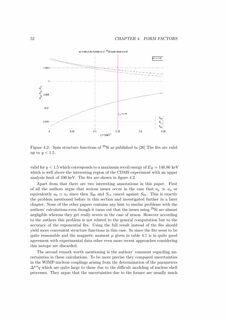
52 CHAPTER 4. FORM FACTORS
Figure 4.2: Spin structure functions of 29Si as published in [26] The fits are validup to y < 1.5.
valid for y < 1.5 which corresponds to a maximum recoil energy of ER = 140.86 keVwhich is well above the interesting region of the CDMS experiment with an upperanalysis limit of 100 keV. The fits are shown in figure 4.2.
Apart from that there are two interesting annotations in this paper. Firstof all the authors argue that serious issues occur in the case that ap an orequivalently a0 ' a1 since then S00 and S11 cancel against S01. This is exactlythe problem mentioned before in this section and investigated further in a laterchapter. None of the other papers contains any hint to similar problems with theauthors’ calculations even though it turns out that the issues using 29Si are almostnegligible whereas they get really severe in the case of xenon. However accordingto the authors this problem is not related to the general computation but to theaccuracy of the exponential fits. Using the full result instead of the fits shouldyield more convenient structure functions in this case. So since the fits seem to bequite reasonable and the magnetic moment µ given in table 4.1 is in quite goodagreement with experimental data other even more recent approaches consideringthis isotope are discarded.
The second remark worth mentioning is the authors’ comment regarding un-certainties in these calculations. To be more precise they compared uncertaintiesin the WIMP-nucleon couplings arising from the determination of the parameters∆p,nq which are quite large to those due to the difficult modeling of nuclear shellprocesses. They argue that the uncertainties due to the former are usually much
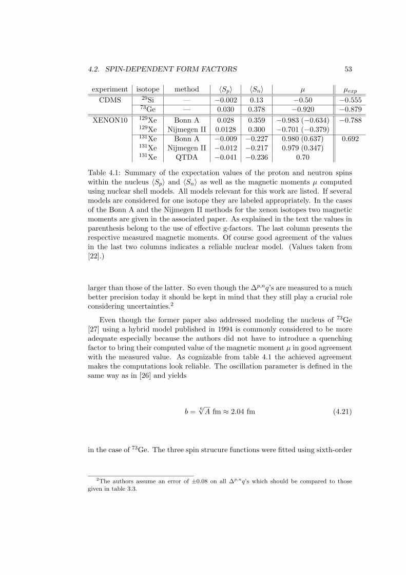
4.2. SPIN-DEPENDENT FORM FACTORS 53
experiment isotope method 〈Sp〉 〈Sn〉 µ µexp
CDMS 29Si — −0.002 0.13 −0.50 −0.55573Ge — 0.030 0.378 −0.920 −0.879
XENON10 129Xe Bonn A 0.028 0.359 −0.983 (−0.634) −0.788129Xe Nijmegen II 0.0128 0.300 −0.701 (−0.379)131Xe Bonn A −0.009 −0.227 0.980 (0.637) 0.692131Xe Nijmegen II −0.012 −0.217 0.979 (0.347)131Xe QTDA −0.041 −0.236 0.70
Table 4.1: Summary of the expectation values of the proton and neutron spinswithin the nucleus 〈Sp〉 and 〈Sn〉 as well as the magnetic moments µ computedusing nuclear shell models. All models relevant for this work are listed. If severalmodels are considered for one isotope they are labeled appropriately. In the casesof the Bonn A and the Nijmegen II methods for the xenon isotopes two magneticmoments are given in the associated paper. As explained in the text the values inparenthesis belong to the use of effective g-factors. The last column presents therespective measured magnetic moments. Of course good agreement of the valuesin the last two columns indicates a reliable nuclear model. (Values taken from[22].)
larger than those of the latter. So even though the ∆p,nq’s are measured to a muchbetter precision today it should be kept in mind that they still play a crucial roleconsidering uncertainties.2
Even though the former paper also addressed modeling the nucleus of 73Ge[27] using a hybrid model published in 1994 is commonly considered to be moreadequate especially because the authors did not have to introduce a quenchingfactor to bring their computed value of the magnetic moment µ in good agreementwith the measured value. As cognizable from table 4.1 the achieved agreementmakes the computations look reliable. The oscillation parameter is defined in thesame way as in [26] and yields
b = 6√A fm ≈ 2.04 fm (4.21)
in the case of 73Ge. The three spin strucure functions were fitted using sixth-order
2The authors assume an error of ±0.08 on all ∆p,nq’s which should be compared to thosegiven in table 3.3.
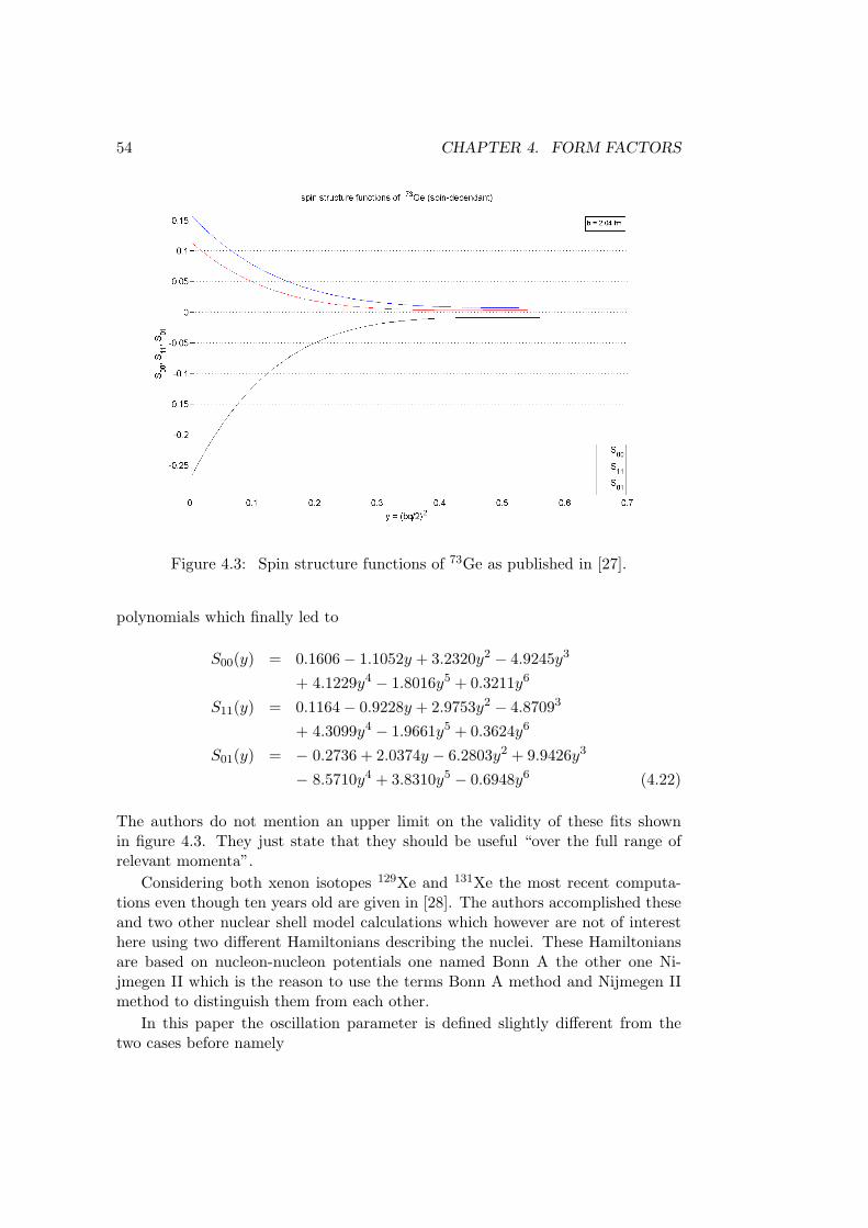
54 CHAPTER 4. FORM FACTORS
Figure 4.3: Spin structure functions of 73Ge as published in [27].
polynomials which finally led to
S00(y) = 0.1606− 1.1052y + 3.2320y2 − 4.9245y3
+ 4.1229y4 − 1.8016y5 + 0.3211y6
S11(y) = 0.1164− 0.9228y + 2.9753y2 − 4.87093
+ 4.3099y4 − 1.9661y5 + 0.3624y6
S01(y) = − 0.2736 + 2.0374y − 6.2803y2 + 9.9426y3
− 8.5710y4 + 3.8310y5 − 0.6948y6 (4.22)
The authors do not mention an upper limit on the validity of these fits shownin figure 4.3. They just state that they should be useful “over the full range ofrelevant momenta”.
Considering both xenon isotopes 129Xe and 131Xe the most recent computa-tions even though ten years old are given in [28]. The authors accomplished theseand two other nuclear shell model calculations which however are not of interesthere using two different Hamiltonians describing the nuclei. These Hamiltoniansare based on nucleon-nucleon potentials one named Bonn A the other one Ni-jmegen II which is the reason to use the terms Bonn A method and Nijmegen IImethod to distinguish them from each other.
In this paper the oscillation parameter is defined slightly different from thetwo cases before namely
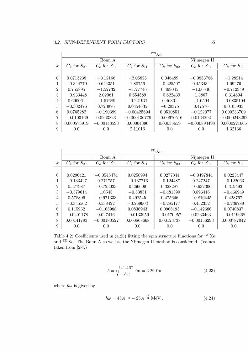
4.2. SPIN-DEPENDENT FORM FACTORS 55
129XeBonn A Nijmegen II
k Ck for S00 Ck for S01 Ck for S11 Ck for S00 Ck for S01 Ck for S11
0 0.0713238 −0.12166 −2.05825 0.046489 −0.0853786 −1.282141 −0.344779 0.644351 1.80756 −0.225507 0.453434 1.092762 0.755895 −1.52732 −1.27746 0.499045 −1.06546 −0.7129493 −0.933448 2.02061 0.654589 −0.622439 1.3867 0.3148944 0.690061 −1.57689 −0.221971 0.46361 −1.0594 −0.08351045 −0.302476 0.723976 0.0454635 −0.20375 0.47576 0.01059336 0.0765282 −0.190399 −0.00425694 0.0510851 −0.122077 0.0002337097 −0.0103169 0.0263823 −0.000136779 −0.00670516 0.0164292 −0.0002432928 0.000573919 −0.00148593 0.00004396 0.00035659 −0.000894498 0.00002216669 0.0 0.0 2.11016 0.0 0.0 1.32136
131XeBonn A Nijmegen II
k Ck for S00 Ck for S01 Ck for S11 Ck for S00 Ck for S01 Ck for S11
0 0.0296421 −0.0545474 0.0250994 0.0277344 −0.0497844 0.02234471 −0.133427 0.271757 −0.137716 −0.124487 0.247247 −0.1220632 0.377987 −0.723023 0.366609 0.328287 −0.632306 0.3194933 −0.579614 1.0545 −0.53851 −0.481399 0.896416 −0.4669494 0.578896 −0.971333 0.492545 0.475646 −0.816445 0.4287675 −0.345562 0.538422 −0.269903 −0.285177 0.452352 −0.2367896 0.115952 −0.168988 0.0836943 0.0968193 −0.142686 0.07408377 −0.0201178 0.027416 −0.0133959 −0.0170957 0.0233463 −0.01196688 0.00141793 −0.00180527 0.000868668 0.00123738 −0.00156293 0.0007870429 0.0 0.0 0.0 0.0 0.0 0.0
Table 4.2: Coefficients used in (4.25) fitting the spin structure functions for 129Xeand 131Xe. The Bonn A as well as the Nijmegen II method is considered. (Valuestaken from [28].)
b =
√41.467
~ωfm = 2.29 fm (4.23)
where ~ω is given by
~ω = 45A−13 − 25A−
23 MeV . (4.24)
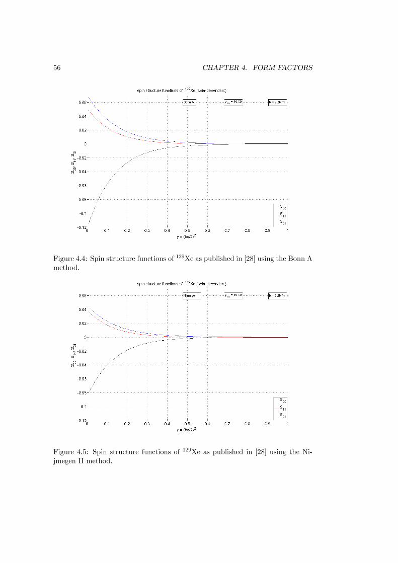
56 CHAPTER 4. FORM FACTORS
Figure 4.4: Spin structure functions of 129Xe as published in [28] using the Bonn Amethod.
Figure 4.5: Spin structure functions of 129Xe as published in [28] using the Ni-jmegen II method.
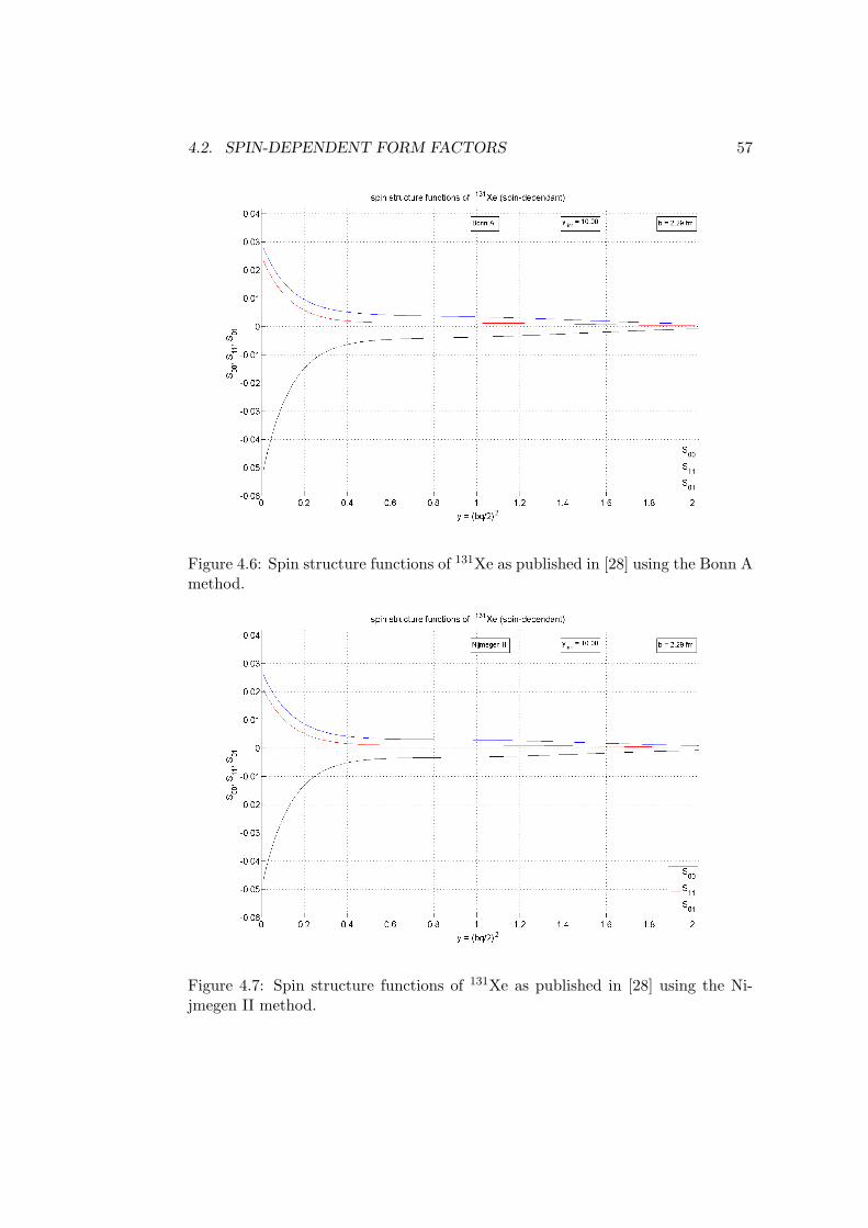
4.2. SPIN-DEPENDENT FORM FACTORS 57
Figure 4.6: Spin structure functions of 131Xe as published in [28] using the Bonn Amethod.
Figure 4.7: Spin structure functions of 131Xe as published in [28] using the Ni-jmegen II method.
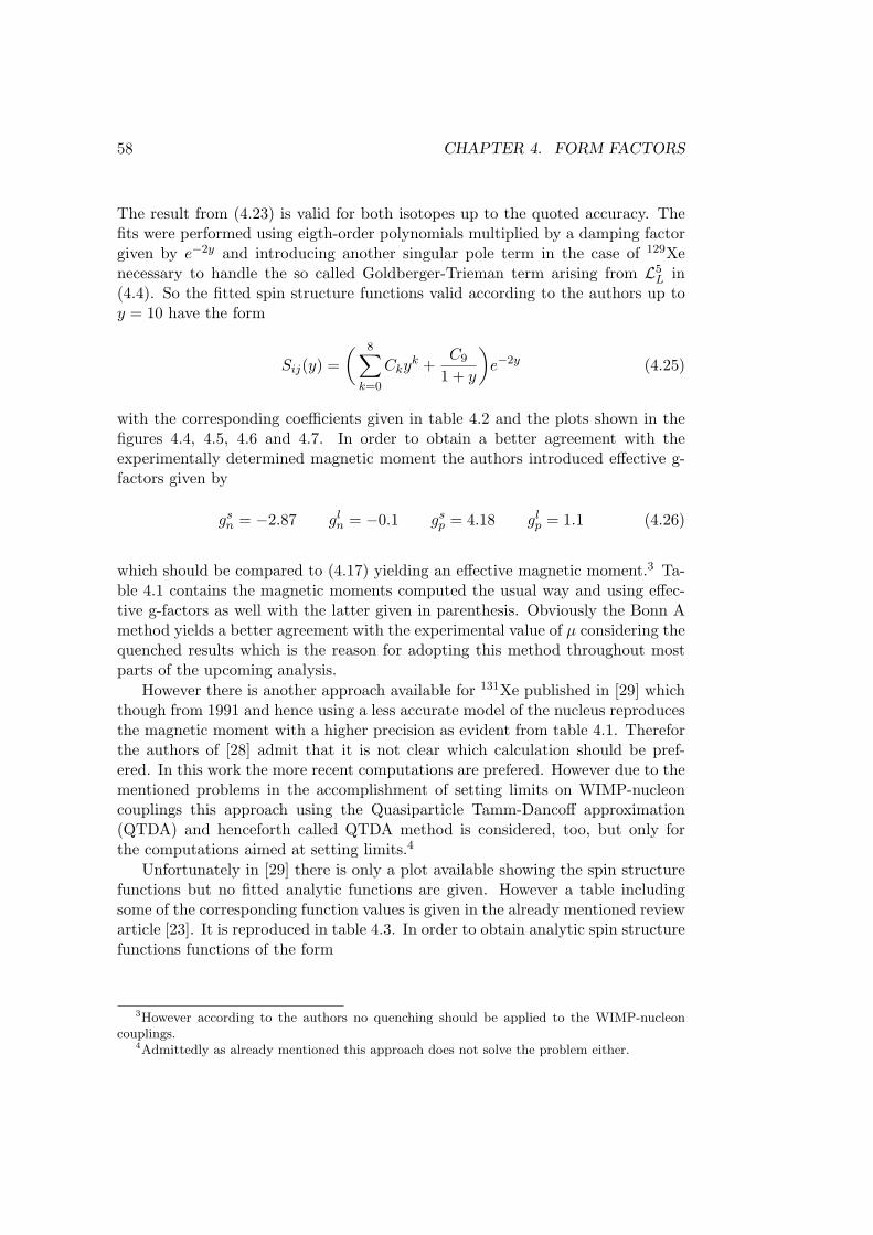
58 CHAPTER 4. FORM FACTORS
The result from (4.23) is valid for both isotopes up to the quoted accuracy. Thefits were performed using eigth-order polynomials multiplied by a damping factorgiven by e−2y and introducing another singular pole term in the case of 129Xenecessary to handle the so called Goldberger-Trieman term arising from L5
L in(4.4). So the fitted spin structure functions valid according to the authors up toy = 10 have the form
Sij(y) =( 8∑k=0
Ckyk +
C9
1 + y
)e−2y (4.25)
with the corresponding coefficients given in table 4.2 and the plots shown in thefigures 4.4, 4.5, 4.6 and 4.7. In order to obtain a better agreement with theexperimentally determined magnetic moment the authors introduced effective g-factors given by
gsn = −2.87 gln = −0.1 gsp = 4.18 glp = 1.1 (4.26)
which should be compared to (4.17) yielding an effective magnetic moment.3 Ta-ble 4.1 contains the magnetic moments computed the usual way and using effec-tive g-factors as well with the latter given in parenthesis. Obviously the Bonn Amethod yields a better agreement with the experimental value of µ considering thequenched results which is the reason for adopting this method throughout mostparts of the upcoming analysis.
However there is another approach available for 131Xe published in [29] whichthough from 1991 and hence using a less accurate model of the nucleus reproducesthe magnetic moment with a higher precision as evident from table 4.1. Thereforthe authors of [28] admit that it is not clear which calculation should be pref-ered. In this work the more recent computations are prefered. However due to thementioned problems in the accomplishment of setting limits on WIMP-nucleoncouplings this approach using the Quasiparticle Tamm-Dancoff approximation(QTDA) and henceforth called QTDA method is considered, too, but only forthe computations aimed at setting limits.4
Unfortunately in [29] there is only a plot available showing the spin structurefunctions but no fitted analytic functions are given. However a table includingsome of the corresponding function values is given in the already mentioned reviewarticle [23]. It is reproduced in table 4.3. In order to obtain analytic spin structurefunctions functions of the form
3However according to the authors no quenching should be applied to the WIMP-nucleoncouplings.
4Admittedly as already mentioned this approach does not solve the problem either.
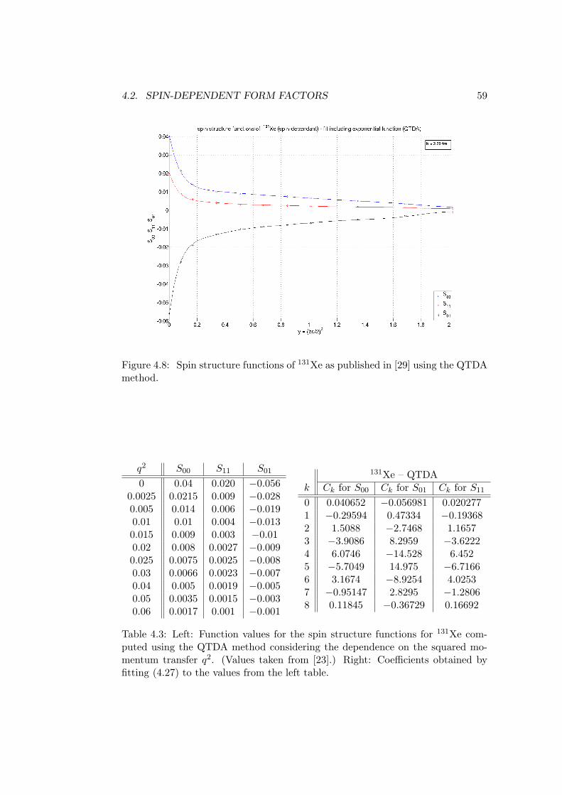
4.2. SPIN-DEPENDENT FORM FACTORS 59
Figure 4.8: Spin structure functions of 131Xe as published in [29] using the QTDAmethod.
q2 S00 S11 S01
0 0.04 0.020 −0.0560.0025 0.0215 0.009 −0.0280.005 0.014 0.006 −0.0190.01 0.01 0.004 −0.0130.015 0.009 0.003 −0.010.02 0.008 0.0027 −0.0090.025 0.0075 0.0025 −0.0080.03 0.0066 0.0023 −0.0070.04 0.005 0.0019 −0.0050.05 0.0035 0.0015 −0.0030.06 0.0017 0.001 −0.001
131Xe – QTDAk Ck for S00 Ck for S01 Ck for S11
0 0.040652 −0.056981 0.0202771 −0.29594 0.47334 −0.193682 1.5088 −2.7468 1.16573 −3.9086 8.2959 −3.62224 6.0746 −14.528 6.4525 −5.7049 14.975 −6.71666 3.1674 −8.9254 4.02537 −0.95147 2.8295 −1.28068 0.11845 −0.36729 0.16692
Table 4.3: Left: Function values for the spin structure functions for 131Xe com-puted using the QTDA method considering the dependence on the squared mo-mentum transfer q2. (Values taken from [23].) Right: Coefficients obtained byfitting (4.27) to the values from the left table.
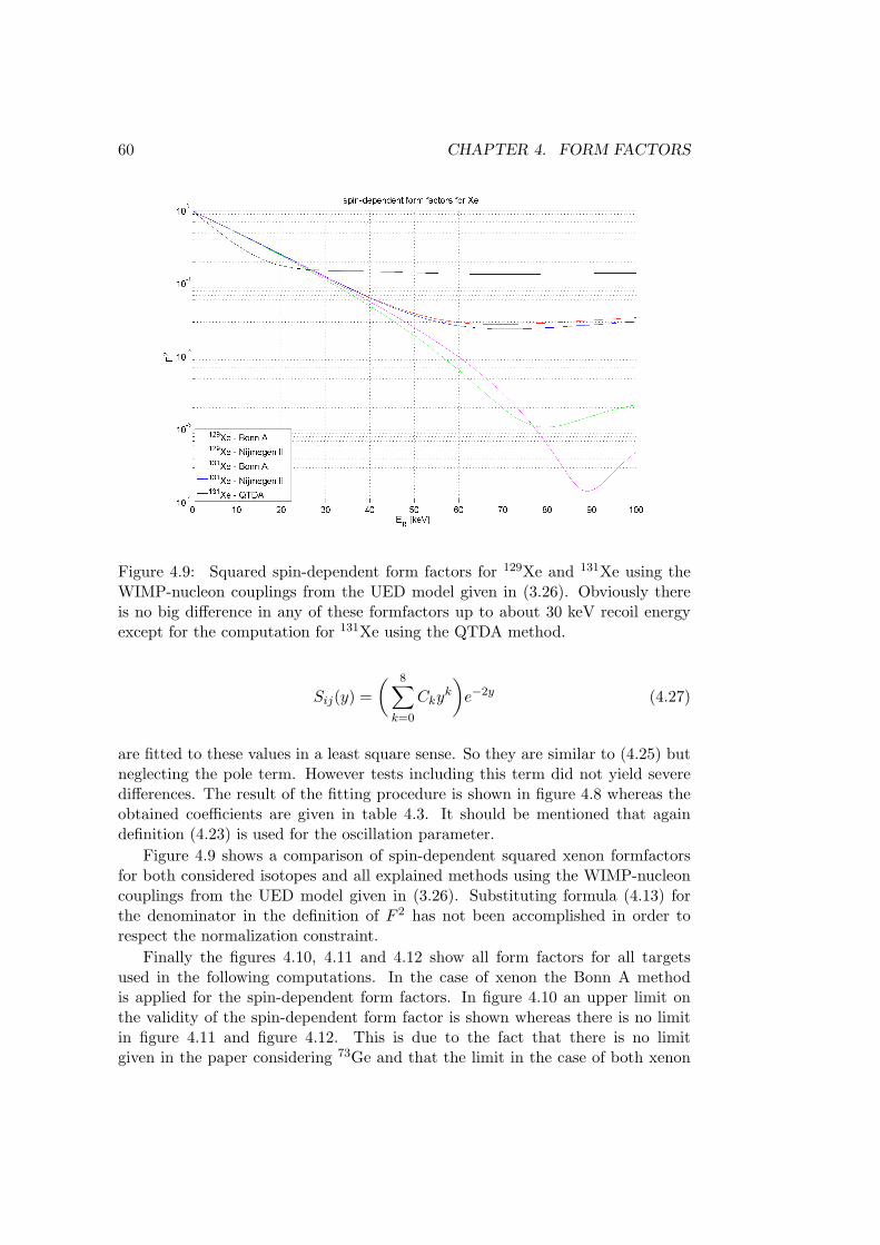
60 CHAPTER 4. FORM FACTORS
Figure 4.9: Squared spin-dependent form factors for 129Xe and 131Xe using theWIMP-nucleon couplings from the UED model given in (3.26). Obviously thereis no big difference in any of these formfactors up to about 30 keV recoil energyexcept for the computation for 131Xe using the QTDA method.
Sij(y) =( 8∑k=0
Ckyk
)e−2y (4.27)
are fitted to these values in a least square sense. So they are similar to (4.25) butneglecting the pole term. However tests including this term did not yield severedifferences. The result of the fitting procedure is shown in figure 4.8 whereas theobtained coefficients are given in table 4.3. It should be mentioned that againdefinition (4.23) is used for the oscillation parameter.
Figure 4.9 shows a comparison of spin-dependent squared xenon formfactorsfor both considered isotopes and all explained methods using the WIMP-nucleoncouplings from the UED model given in (3.26). Substituting formula (4.13) forthe denominator in the definition of F 2 has not been accomplished in order torespect the normalization constraint.
Finally the figures 4.10, 4.11 and 4.12 show all form factors for all targetsused in the following computations. In the case of xenon the Bonn A methodis applied for the spin-dependent form factors. In figure 4.10 an upper limit onthe validity of the spin-dependent form factor is shown whereas there is no limitin figure 4.11 and figure 4.12. This is due to the fact that there is no limitgiven in the paper considering 73Ge and that the limit in the case of both xenon
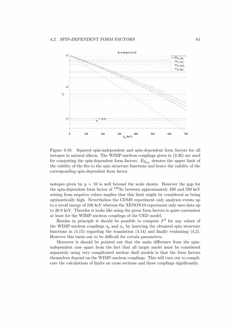
4.2. SPIN-DEPENDENT FORM FACTORS 61
Figure 4.10: Squared spin-independent and spin-dependent form factors for allisotopes in natural silicon. The WIMP-nucleon couplings given in (3.26) are usedfor computing the spin-dependent form factors. ERlim
denotes the upper limit ofthe validity of the fits to the spin structure functions and hence the validity of thecorresponding spin-dependent form factor.
isotopes given by y = 10 is well beyond the scale shown. However the gap forthe spin-dependent form factor of 129Xe between approximately 420 and 520 keVarising from negative values implies that this limit might be considered as beingoptimistically high. Nevertheless the CDMS experiment only analyzes events upto a recoil energy of 100 keV whereas the XENON10 experiment only uses data upto 26.9 keV. Therefor it looks like using the given form factors is quite convenientat least for the WIMP-nucleon couplings of the UED model.
Besides in principle it should be possible to compute F 2 for any values ofthe WIMP-nucleon couplings ap and an by inserting the obtained spin structurefunctions in (4.15) regarding the translation (4.14) and finally evaluating (4.2).However this turns out to be difficult for certain parameters.
Moreover it should be pointed out that the main difference from the spin-independent case apart from the fact that all target nuclei must be consideredseparately using very complicated nuclear shell models is that the form factorsthemselves depend on the WIMP-nucleon couplings. This will turn out to compli-cate the calculations of limits on cross sections and these couplings significantly.
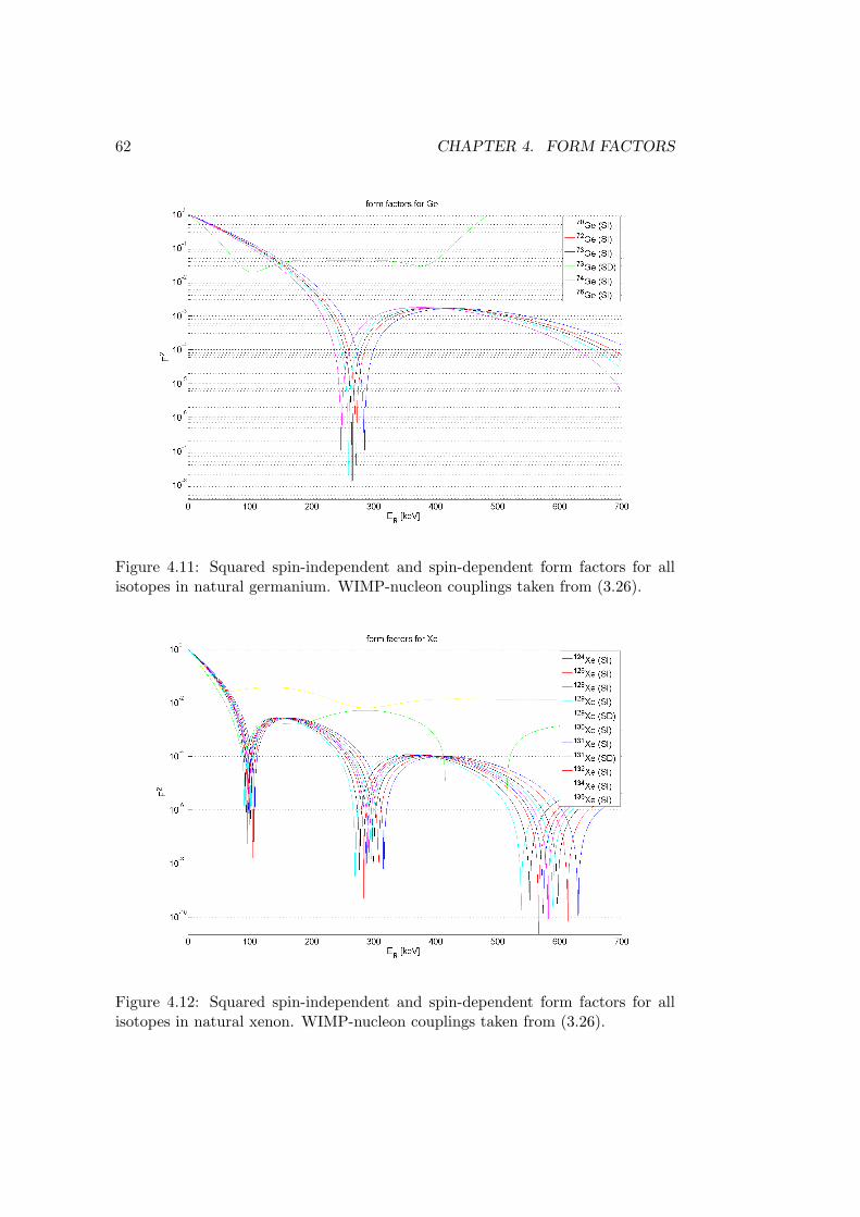
62 CHAPTER 4. FORM FACTORS
Figure 4.11: Squared spin-independent and spin-dependent form factors for allisotopes in natural germanium. WIMP-nucleon couplings taken from (3.26).
Figure 4.12: Squared spin-independent and spin-dependent form factors for allisotopes in natural xenon. WIMP-nucleon couplings taken from (3.26).
Chapter 5
Event rates from B(1)-nucleiscattering
After these extensive investigations of the spin-independent and spin-dependentB(1)-nuclei zero-momentum transfer cross sections and appropriate form factorsto include the finite-momentum transfer all necessary information are available tocompute theoretical predictions for expected event rates. The standard referencefor this procedure is [24] which gives an excellent summary of this topic.
To come to grips with this problem it is necessary to make certain assumptionsabout the dark matter halo. It is a common procedure to assume an isothermaland isotropic sphere of WIMP gas obeying a yet to define velocity dispersion. Un-fortunately reliability of this assumption is not secured at all. However detailedanalysis shows that the uncertainties in modelizing the halo are rather small com-pared for example to theoretical uncertainties arising from calculations of theWIMP-nucleon cross sections.
However before actually proceeding with this issue it is convenient to discusstwo other short topics first because they are important for the following calcula-tions.
The first one is the velocity of the earth with respect to the galactic rest framevE which is its relative velocity to the motionless dark matter halo introducedabove at the same time. In fact there are three contributions to this velocitynamely the galactic rotation velocity ~vr, the velocity of the sun with respect to themoving galactic disc ~vs which can be measured by investigating its motion relativeto nearby stars and finally the velocity of the earth arising from its motion aroundthe sun ~vorb. So it can be written as
~vE = ~vr + ~vs + ~vorb . (5.1)
Using galactic coordinates the first two contributions are given by
63
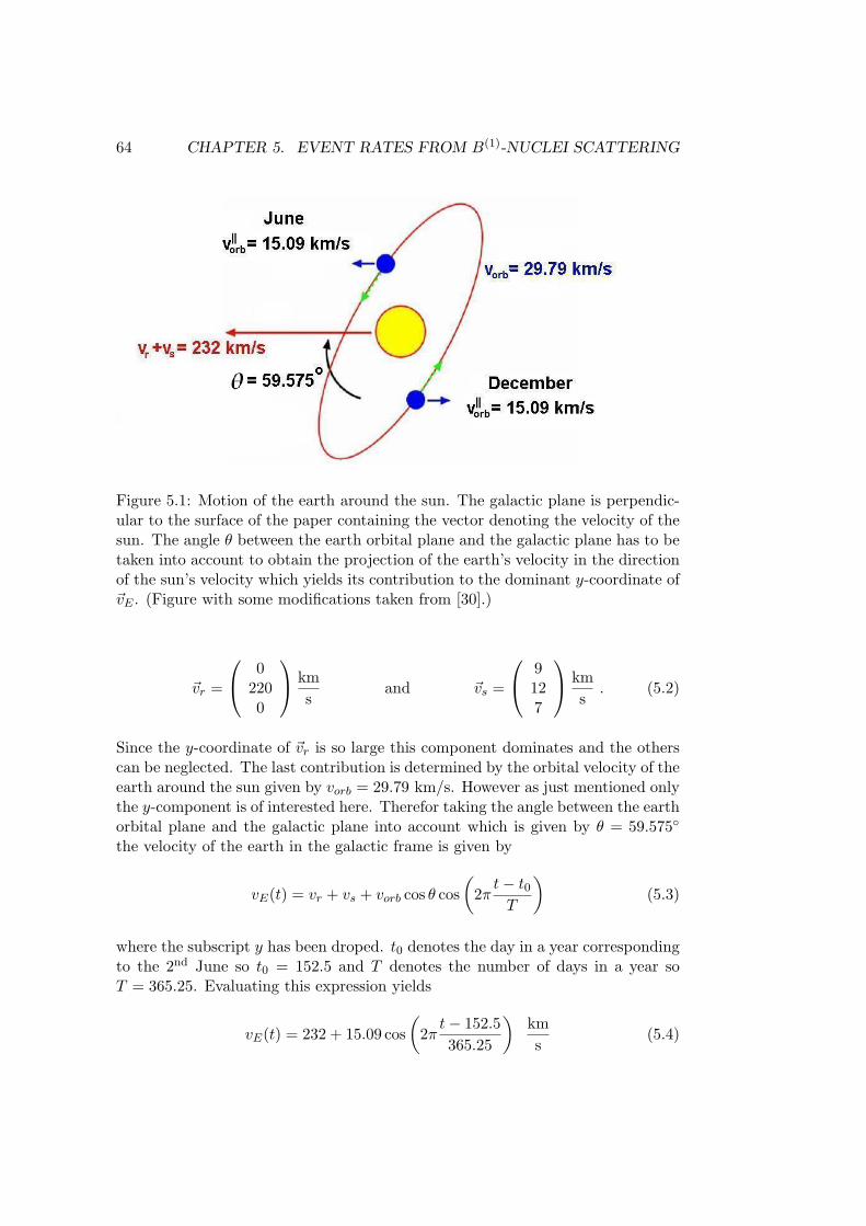
64 CHAPTER 5. EVENT RATES FROM B(1)-NUCLEI SCATTERING
Figure 5.1: Motion of the earth around the sun. The galactic plane is perpendic-ular to the surface of the paper containing the vector denoting the velocity of thesun. The angle θ between the earth orbital plane and the galactic plane has to betaken into account to obtain the projection of the earth’s velocity in the directionof the sun’s velocity which yields its contribution to the dominant y-coordinate of~vE . (Figure with some modifications taken from [30].)
~vr =
02200
kms
and ~vs =
9127
kms
. (5.2)
Since the y-coordinate of ~vr is so large this component dominates and the otherscan be neglected. The last contribution is determined by the orbital velocity of theearth around the sun given by vorb = 29.79 km/s. However as just mentioned onlythe y-component is of interested here. Therefor taking the angle between the earthorbital plane and the galactic plane into account which is given by θ = 59.575
the velocity of the earth in the galactic frame is given by
vE(t) = vr + vs + vorb cos θ cos(
2πt− t0T
)(5.3)
where the subscript y has been droped. t0 denotes the day in a year correspondingto the 2nd June so t0 = 152.5 and T denotes the number of days in a year soT = 365.25. Evaluating this expression yields
vE(t) = 232 + 15.09 cos(
2πt− 152.5365.25
)kms
(5.4)
65
which is illustrated in figure 5.1. Obviously this oscillation leads to a modulationof the mean velocity ∼ ±6.5%. It should be pointed out that the mean velocity of232 km/s is burdened with a quite high degree of uncertainty of about ±30 km/swhereas the 15.09 km/s amplitude of the modulation has negligible uncertainty.Moreover note that the modulation is not exactly sinusoidal.
In order to investigate effects caused by this annual modulation which is ac-complished in the next chapter t is taken as a free parameter. However to comparetheoretical predictions to the results of measurements from CDMS and XENON10it is more useful to define a mean earth velocity 〈vE〉.
In the case of the CDMS experiment all data of the runs 118 and 119 wereavailable which made it possible to compute a live time weighted mean by
〈vE〉 =
∑n
vE(tn) ln∑n
ln= 232.2
kms
(5.5)
where the index n runs over all detected events and tn and ln denote the event timeand the live time of the nth event respectively. The result which is almost equal tothe mean of vE averaged over a year given by 232 km/s is plausible considering thefact that run 118 lasted from October 11, 2003 until January 11, 2004 as statedin [31] whereas run 119 took data between March 25, 2004 and August 8, 2004 asstated in [32].
Considering the XENON10 experiment only the dates of the beginning and theend of the last run were available. According two [20] data were aquired betweenOctober 6, 2006 and February 14, 2007. Hence an average velocity was obtainedby evaluating
〈vE〉 =1trun
∫trun
vE(t) dt =1
131.25
(∫ 365.25
279.5vE(t) dt+
∫ 45.5
0vE(t) dt
)= 220.1
kms
.
(5.6)
Obviously trun = 131.25 denotes the duration of the run while 279.5 and 45.5represent the day in the year of its beginning and its ending. The just obtainedresults are summarized in figure 5.2.
The second topic is a short discussion of the local dark matter density ρWwhich is of importance in the upcoming computations. Several groups have tried torestrict its value. An example is given in [34]. The authors started by constructinga large variety of models based on some fundamental ingredients like a bar or anasymmetric bulge, a disk with certain properties and isothermal cold dark matterand MACHO halos with finite radii and ellipsoidal density profiles. Then severalparameters like the bulge mass and the halo radii were varied. Finally all modelswere rejected which did not give rise to certain measured values of for example
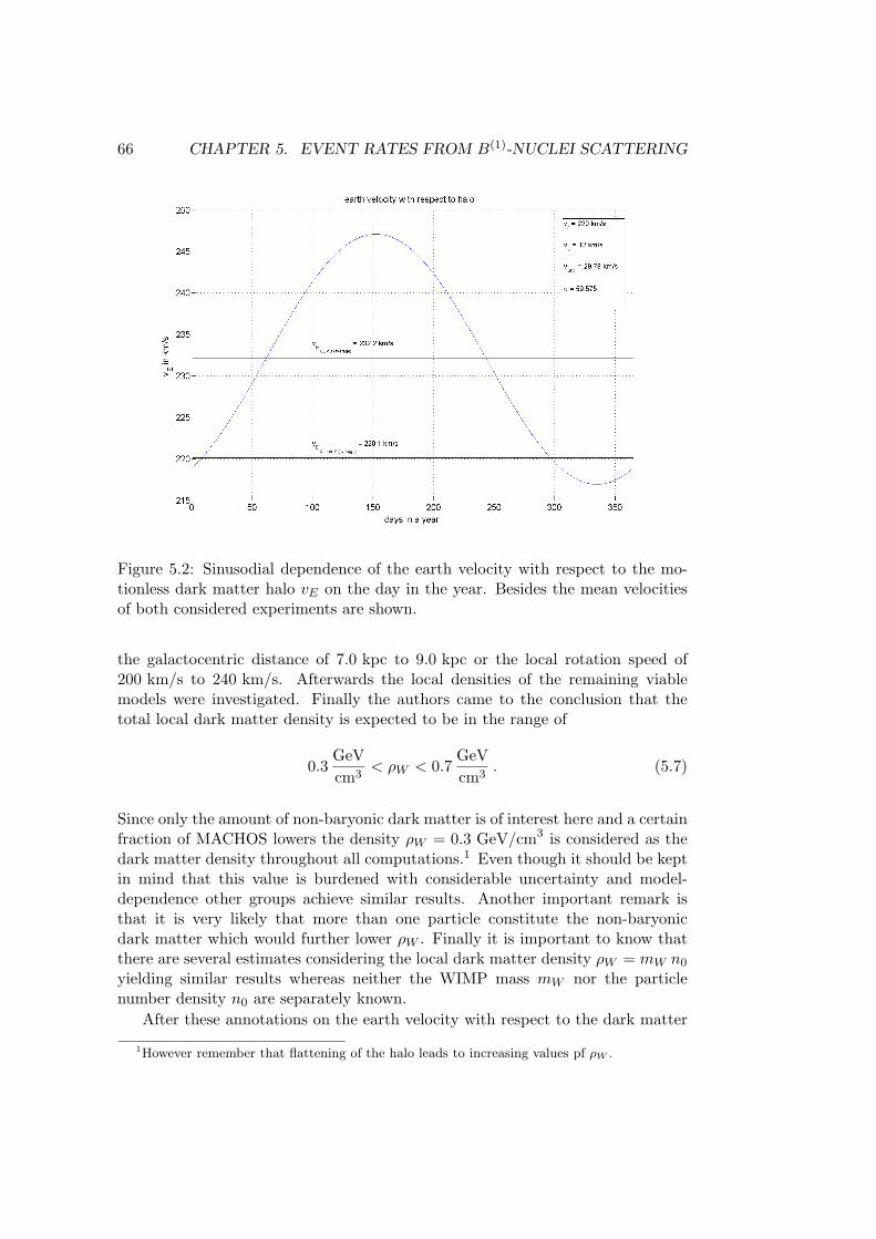
66 CHAPTER 5. EVENT RATES FROM B(1)-NUCLEI SCATTERING
Figure 5.2: Sinusodial dependence of the earth velocity with respect to the mo-tionless dark matter halo vE on the day in the year. Besides the mean velocitiesof both considered experiments are shown.
the galactocentric distance of 7.0 kpc to 9.0 kpc or the local rotation speed of200 km/s to 240 km/s. Afterwards the local densities of the remaining viablemodels were investigated. Finally the authors came to the conclusion that thetotal local dark matter density is expected to be in the range of
0.3GeVcm3
< ρW < 0.7GeVcm3
. (5.7)
Since only the amount of non-baryonic dark matter is of interest here and a certainfraction of MACHOS lowers the density ρW = 0.3 GeV/cm3 is considered as thedark matter density throughout all computations.1 Even though it should be keptin mind that this value is burdened with considerable uncertainty and model-dependence other groups achieve similar results. Another important remark isthat it is very likely that more than one particle constitute the non-baryonicdark matter which would further lower ρW . Finally it is important to know thatthere are several estimates considering the local dark matter density ρW = mW n0
yielding similar results whereas neither the WIMP mass mW nor the particlenumber density n0 are separately known.
After these annotations on the earth velocity with respect to the dark matter
1However remember that flattening of the halo leads to increasing values pf ρW .
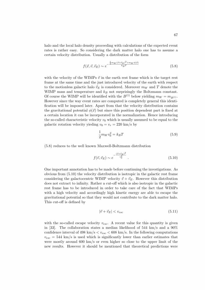
67
halo and the local halo density proceeding with calculations of the expected eventrates is rather easy. So considering the dark matter halo one has to assume acertain velocity distribution. Usually a distribution of the form
f(~x,~v,~vE) ∼ e−12mW (~v+~vE)2+mWφ(~x)
kBT (5.8)
with the velocity of the WIMPs ~v in the earth rest frame which is the target restframe at the same time and the just introduced velocity of the earth with respectto the motionless galactic halo ~vE is considered. Moreover mW and T denote theWIMP mass and temperature and kB not surprisingly the Boltzmann constant.Of course the WIMP will be identified with the B(1) below yielding mW = mB(1) .However since the way event rates are computed is completely general this identi-fication will be imposed later. Apart from that the velocity distribution containsthe gravitational potential φ(~x) but since this position dependent part is fixed ata certain location it can be incorporated in the normalization. Hence introducingthe so-called characteristic velocity v0 which is usually assumed to be equal to thegalactic rotation velocity yieding v0 = vr = 220 km/s by
12mW v
20 = kBT (5.9)
(5.8) reduces to the well known Maxwell-Boltzmann distribution
f(~v,~vE) ∼ e− (~v+~vE)2
v20 . (5.10)
One important annotation has to be made before continuing the investigations. Asobvious from (5.10) the velocity distribution is isotropic in the galactic rest frameconsidering the galactocentric WIMP velocity ~v + ~vE . However this distributiondoes not extract to infinity. Rather a cut-off which is also isotropic in the galacticrest frame has to be introduced in order to take care of the fact that WIMPswith a high velocity and accordingly high kinetic energy are able to escape thegravitational potential so that they would not contribute to the dark matter halo.This cut-off is defined by
|~v + ~vE | < vesc (5.11)
with the so-called escape velocity vesc. A recent value for this quantity is givenin [33]. The collaboration states a median likelihood of 544 km/s and a 90%confidence interval of 498 km/s < vesc < 608 km/s. In the following computationsvesc = 544 km/s is used which is significantly lower than earlier estimates thatwere mostly around 600 km/s or even higher so close to the upper limit of thenew results. However it should be mentioned that theoretical predictions were
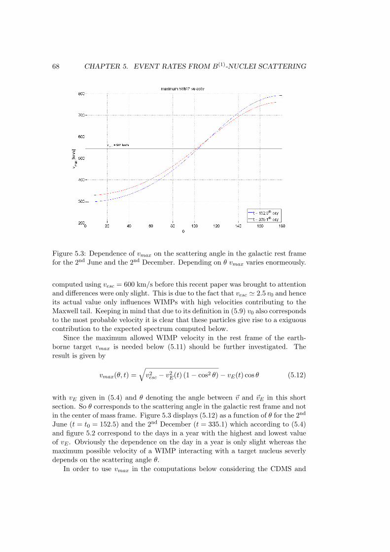
68 CHAPTER 5. EVENT RATES FROM B(1)-NUCLEI SCATTERING
Figure 5.3: Dependence of vmax on the scattering angle in the galactic rest framefor the 2nd June and the 2nd December. Depending on θ vmax varies enormeously.
computed using vesc = 600 km/s before this recent paper was brought to attentionand differences were only slight. This is due to the fact that vesc ' 2.5 v0 and henceits actual value only influences WIMPs with high velocities contributing to theMaxwell tail. Keeping in mind that due to its definition in (5.9) v0 also correspondsto the most probable velocity it is clear that these particles give rise to a exiguouscontribution to the expected spectrum computed below.
Since the maximum allowed WIMP velocity in the rest frame of the earth-borne target vmax is needed below (5.11) should be further investigated. Theresult is given by
vmax(θ, t) =√v2esc − v2
E(t) (1− cos2 θ)− vE(t) cos θ (5.12)
with vE given in (5.4) and θ denoting the angle between ~v and ~vE in this shortsection. So θ corresponds to the scattering angle in the galactic rest frame and notin the center of mass frame. Figure 5.3 displays (5.12) as a function of θ for the 2nd
June (t = t0 = 152.5) and the 2nd December (t = 335.1) which according to (5.4)and figure 5.2 correspond to the days in a year with the highest and lowest valueof vE . Obviously the dependence on the day in a year is only slight whereas themaximum possible velocity of a WIMP interacting with a target nucleus severlydepends on the scattering angle θ.
In order to use vmax in the computations below considering the CDMS and
69
XENON10 experiment it is useful to define a mean maximum velocity 〈vmax〉similar to 〈vE〉. This is accomplished by substituting vE(t) in (5.12) by 〈vE〉 givenin (5.5) in the case of CDMS and (5.6) in the case of XENON10. Afterwards anaveraging over the scattering angle is excecuted so that 〈vmax〉 is definded by
〈vmax〉 =1π
∫ π
0
(√v2esc − 〈vE〉2 (1− cos2 θ)− 〈vE〉 cos θ
)dθ (5.13)
leading to 〈vmax〉 = 518.3 km/s for the CDMS experiment and 〈vmax〉 = 521.0 km/sfor the XENON10 experiment.
In order to actually adress the problem of event rates it is necessary to takea short look at the kinematics which is very instructive at the same time sinceit yields an idea about the energies involved in the scattering processes. Thiscan be accomplished by considering simple Newtonian mechanics. Obviously thisassumption is valid since only WIMPs with a velocity up to vesc are considered. Soassuming the WIMP-nuclei interaction to be a simple scattering process applyingenergy and momentum conservation directly yields
ER =12Er(1− cos θ) (5.14)
with the WIMP energy E, the recoil energy ER and the so-called kinematic factor
r =4mWmT
(mW +mT )2. (5.15)
Moreover it is important to know that in this context θ denotes the scatteringangle in the centre-of-mass frame. Since the non-relativistic limit is considered Eis simply given by
E =12mW v
2 . (5.16)
So what is the magnitude of the expected recoil energy? This can be estimatedby making some appropriate assumptions about the WIMP mass and its velocity.Obvioulsy a mass of mW = 500 GeV consistent with the results from relic densitycomputations shown in figure 2.6 and a velocity of v = v0 = 220 km/s seems quitereasonable. Evaluating (5.16) yields an energy carried by the WIMP of aboutE = 135 keV. Considering scattering from a 73Ge nuclei with mT = 68 GeVyields a kinematic factor of r = 0.4 and hence according to (5.14) an expectedrecoil energy of about ER ' Er = 57 keV. Obviously the expected recoil energyrange is of order ∼ 10 keV and even smaller for lighter WIMPs.
According to (5.14) and (5.16) the maximum recoil energy ERmax is given by
ERmax =12mW v
2maxr (5.17)
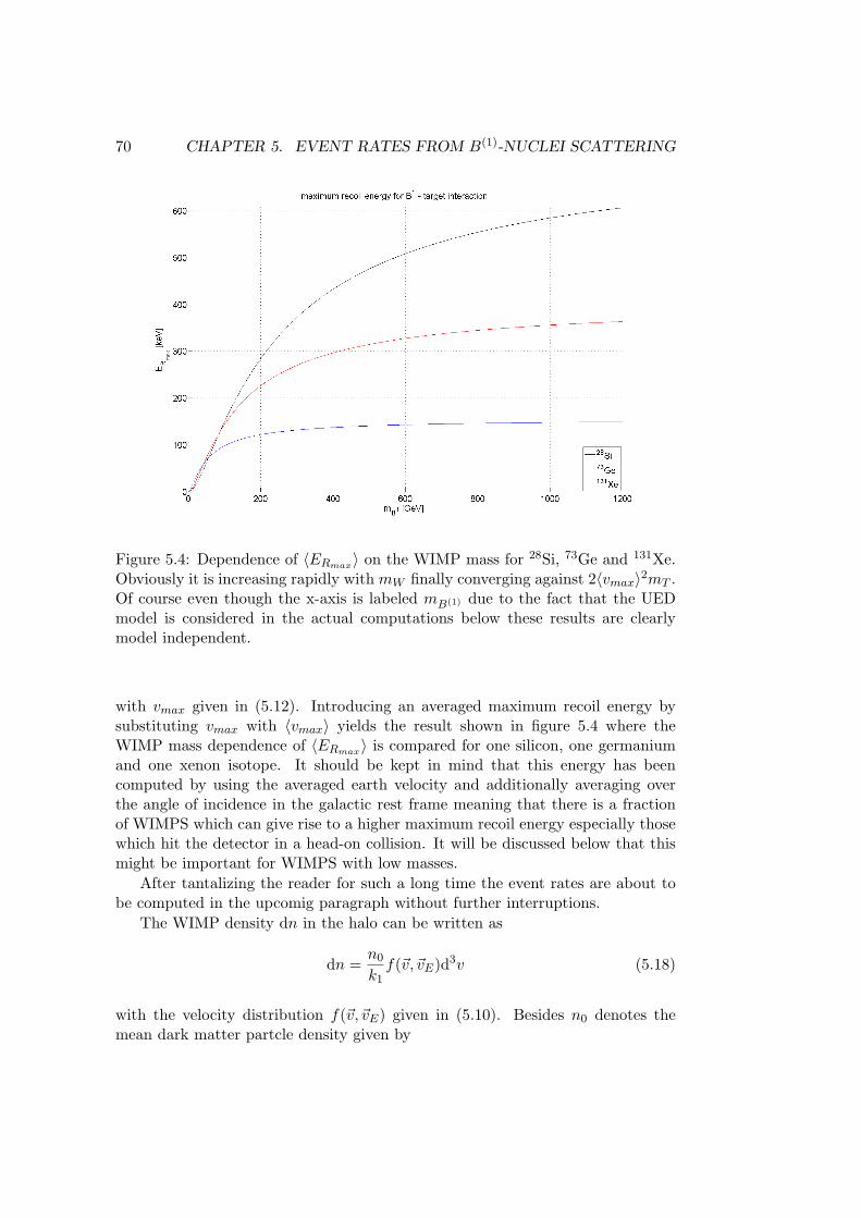
70 CHAPTER 5. EVENT RATES FROM B(1)-NUCLEI SCATTERING
Figure 5.4: Dependence of 〈ERmax〉 on the WIMP mass for 28Si, 73Ge and 131Xe.Obviously it is increasing rapidly with mW finally converging against 2〈vmax〉2mT .Of course even though the x-axis is labeled mB(1) due to the fact that the UEDmodel is considered in the actual computations below these results are clearlymodel independent.
with vmax given in (5.12). Introducing an averaged maximum recoil energy bysubstituting vmax with 〈vmax〉 yields the result shown in figure 5.4 where theWIMP mass dependence of 〈ERmax〉 is compared for one silicon, one germaniumand one xenon isotope. It should be kept in mind that this energy has beencomputed by using the averaged earth velocity and additionally averaging overthe angle of incidence in the galactic rest frame meaning that there is a fractionof WIMPS which can give rise to a higher maximum recoil energy especially thosewhich hit the detector in a head-on collision. It will be discussed below that thismight be important for WIMPS with low masses.
After tantalizing the reader for such a long time the event rates are about tobe computed in the upcomig paragraph without further interruptions.
The WIMP density dn in the halo can be written as
dn =n0
k1f(~v,~vE)d3v (5.18)
with the velocity distribution f(~v,~vE) given in (5.10). Besides n0 denotes themean dark matter partcle density given by
71
n0 =ρWmW
(5.19)
obeying
n0 =∫ vmax
0dn (5.20)
with ρ = 0.3 GeV/cm3 while k1 denotes the normalization constant. This constantis obviously given by
k1 =∫|~v|<vmax(θ)
f(~v,~vE)d3v =∫ vmax(θ)
0dv v2
∫dΩv e
− (~v+~vE)2
v20 (5.21)
which is rather complicated to evaluate because vmax defined in (5.12) is a functionof θ^(~v,~vE). However remembering that the velocity distribution is isotropic inthe galactic rest frame and the corresponding definition of the cut-off given in(5.11) it is possible to avoid this difficult integration because obviously k1 can alsobe computed evaluating
k1 =∫|~v+~vE |<vesc
f(~v,~vE)d3|~v + ~vE | =∫ vesc
0d|~v + ~vE | |~v + ~vE |2
∫dΩv e
− (~v+~vE)2
v20 .
(5.22)
Since vesc is constant it is easy to evaluate this integral which leads to
k1 = k0
[erf(vescv0
)− 2√
π
vescv0
e− v
2escv20
](5.23)
where k0 is defined in the same way as k1 but with the integration evaluated forvesc =∞ which leads to
k0 =√π π v3
0 . (5.24)
Besides erf denotes the so-called error function defined as
erf(x) =2√π
∫ x
0du e−u
2. (5.25)
The fact that (5.21) and (5.22) yield the same results which has been explicitelytested is in principle also clear since the particle density should be independent ofthe earth velocity.
72 CHAPTER 5. EVENT RATES FROM B(1)-NUCLEI SCATTERING
The differential event rate dR considering zero-momentum transfer is definedas
dR =N0
Auσ v dn (5.26)
which has to be multiplied by the appropriate form factors discussed extensively inthe last chapter to incorporate the finite-momentum transfer. N0 = 6.022 · 1026kg−1
denotes the Avogadro constant while Au represents the atomic mass in u whichin fact is quite similar to A. Theoretical predictions for the cross sections havealready been extensively described. Inserting (5.18) in (5.26) dR can be rewrittenin the form
dR = R0k0
k1
12πv4
0
v f(~v,~vE)d3v (5.27)
with
R0 =2√π
N0
Au
ρWmW
σ v0 (5.28)
which in fact is the total event rate assuming vE = 0, vesc =∞ and integrating overrecoil energies from ER = 0 to ER = ∞. However in the following computationsit is only used as a convenient abbreviation.
Taking a look at (5.14) and assuming isotropic scattering in the center of massframe it can be assumed that recoils are uniformly distributed in ER over therange from 0 to the maximum recoil energy given by E r. Thus the differentialevent rate with respect to the recoil energy is given by
dRdER
=∫ Emax
Emin
1Er
dR(E) =1E0r
∫ vmax
vmin
v20
v2dR(v) (5.29)
with the θ-dependent maximum velocity vmax given in (5.12) and E0 defined asthe energy carried by a WIMP with velocity v0
E0 =12mW v
20 . (5.30)
Moreover vmin is defined as the minimum velocity leading to a certain recoil energyER which yields
vmin =√
2EminmW
=√ERE0r
v0 (5.31)
since Emin = ERr . Inserting (5.27) into (5.29) leads to
73
dRdER
=R0
E0r
k0
k1
12πv2
0
∫ vmax
vmin
1vf(~v,~vE)d3v . (5.32)
Unfortunately the occuring integration cannot be simplified similar to the waycomputing the normalization constant k1. Therefor the θ-dependence of vmax hasto be carefully regarded. Nevertheless evaluation of the occuring integral finallyyields the rather complicated result
dRdER
=R0
E0r
k0
k1
[√π
4v0
vE
[erf(vmin + vE
v0
)− erf
(vmin − vE
v0
)]− e− v
2escv20
](5.33)
which energy dependence is approximately exponentially decreasing. This be-haviour is evident from considering vE = 0 and vesc =∞ which yields
dRdER
|vesc=∞vE=0 =R0
E0reERE0r (5.34)
It should be kept in mind that this expression depends on the day in the year viavE which will be further discussed below.
Since R0 is proportional to σ the differential rate is proportional to σ as wellwhich is the only part of (5.33) depending on the kind of interaction and hencebeing related to the assumed UED model described in former chapters. Thereforand especially for latter purposes considering limit computations it is convenientto define dR
dER|σ denoting the whole expression given in (5.33) except for the cross
section σ. Using this abbreviation the spin-independent and if applicable the spin-dependent differential event rates including the form factors for finite-momentumtransfer are given by
dRdER
|SI = σSIdR
dER|σ F 2
SI (5.35)
dRdER
|SD = σSDdR
dER|σ F 2
SD . (5.36)
Hence the total differential event rate for scattering from a certain nuclei can becomputed using
dRdER
|total =dR
dER|SI +
dRdER
|SD = σSIdR
dER|σ F 2
SI + σSDdR
dER|σ F 2
SD . (5.37)
Finally if the considered target consists of more than one element which is thecase in both experiments since only natural silicon, germanium and xenon is usedthe respective abundances f have to be taken into account. Admittedly this is
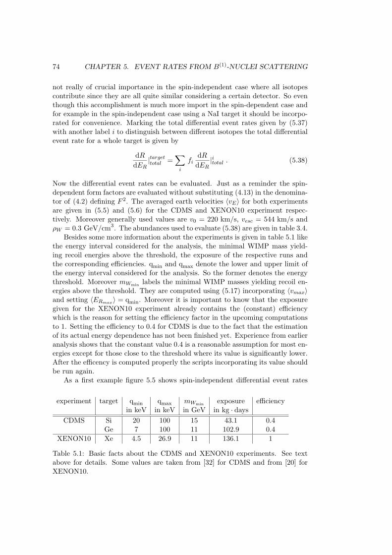
74 CHAPTER 5. EVENT RATES FROM B(1)-NUCLEI SCATTERING
not really of crucial importance in the spin-independent case where all isotopescontribute since they are all quite similar considering a certain detector. So eventhough this accomplishment is much more import in the spin-dependent case andfor example in the spin-independent case using a NaI target it should be incorpo-rated for convenience. Marking the total differential event rates given by (5.37)with another label i to distinguish between different isotopes the total differentialevent rate for a whole target is given by
dRdER
|targettotal =∑i
fidR
dER|itotal . (5.38)
Now the differential event rates can be evaluated. Just as a reminder the spin-dependent form factors are evaluated without substituting (4.13) in the denomina-tor of (4.2) defining F 2. The averaged earth velocities 〈vE〉 for both experimentsare given in (5.5) and (5.6) for the CDMS and XENON10 experiment respec-tively. Moreover generally used values are v0 = 220 km/s, vesc = 544 km/s andρW = 0.3 GeV/cm3. The abundances used to evaluate (5.38) are given in table 3.4.
Besides some more information about the experiments is given in table 5.1 likethe energy interval considered for the analysis, the minimal WIMP mass yield-ing recoil energies above the threshold, the exposure of the respective runs andthe corresponding efficiencies. qmin and qmax denote the lower and upper limit ofthe energy interval considered for the analysis. So the former denotes the energythreshold. Moreover mWmin labels the minimal WIMP masses yielding recoil en-ergies above the threshold. They are computed using (5.17) incorporating 〈vmax〉and setting 〈ERmax〉 = qmin. Moreover it is important to know that the exposuregiven for the XENON10 experiment already contains the (constant) efficiencywhich is the reason for setting the efficiency factor in the upcoming computationsto 1. Setting the efficiency to 0.4 for CDMS is due to the fact that the estimationof its actual energy dependence has not been finished yet. Experience from earlieranalysis shows that the constant value 0.4 is a reasonable assumption for most en-ergies except for those close to the threshold where its value is significantly lower.After the efficency is computed properly the scripts incorporating its value shouldbe run again.
As a first example figure 5.5 shows spin-independent differential event rates
experiment target qmin qmax mWmin exposure efficiencyin keV in keV in GeV in kg · days
CDMS Si 20 100 15 43.1 0.4Ge 7 100 11 102.9 0.4
XENON10 Xe 4.5 26.9 11 136.1 1
Table 5.1: Basic facts about the CDMS and XENON10 experiments. See textabove for details. Some values are taken from [32] for CDMS and from [20] forXENON10.
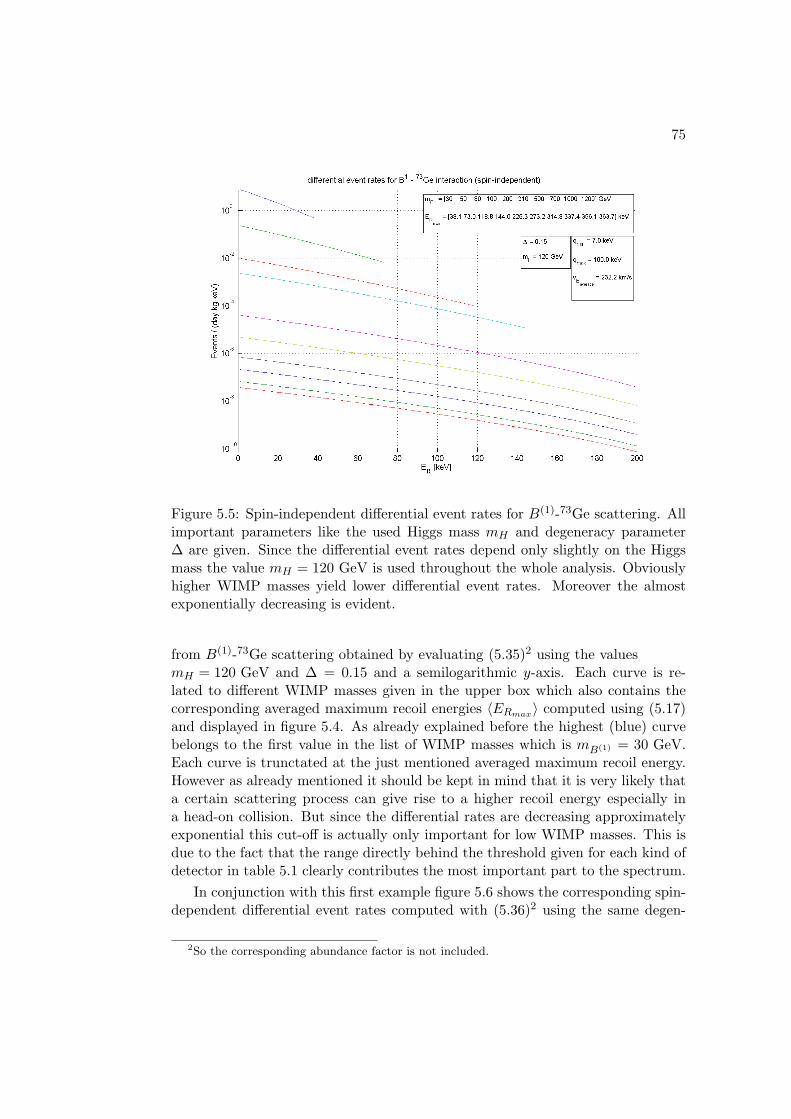
75
Figure 5.5: Spin-independent differential event rates for B(1)-73Ge scattering. Allimportant parameters like the used Higgs mass mH and degeneracy parameter∆ are given. Since the differential event rates depend only slightly on the Higgsmass the value mH = 120 GeV is used throughout the whole analysis. Obviouslyhigher WIMP masses yield lower differential event rates. Moreover the almostexponentially decreasing is evident.
from B(1)-73Ge scattering obtained by evaluating (5.35)2 using the valuesmH = 120 GeV and ∆ = 0.15 and a semilogarithmic y-axis. Each curve is re-lated to different WIMP masses given in the upper box which also contains thecorresponding averaged maximum recoil energies 〈ERmax〉 computed using (5.17)and displayed in figure 5.4. As already explained before the highest (blue) curvebelongs to the first value in the list of WIMP masses which is mB(1) = 30 GeV.Each curve is trunctated at the just mentioned averaged maximum recoil energy.However as already mentioned it should be kept in mind that it is very likely thata certain scattering process can give rise to a higher recoil energy especially ina head-on collision. But since the differential rates are decreasing approximatelyexponential this cut-off is actually only important for low WIMP masses. This isdue to the fact that the range directly behind the threshold given for each kind ofdetector in table 5.1 clearly contributes the most important part to the spectrum.
In conjunction with this first example figure 5.6 shows the corresponding spin-dependent differential event rates computed with (5.36)2 using the same degen-
2So the corresponding abundance factor is not included.
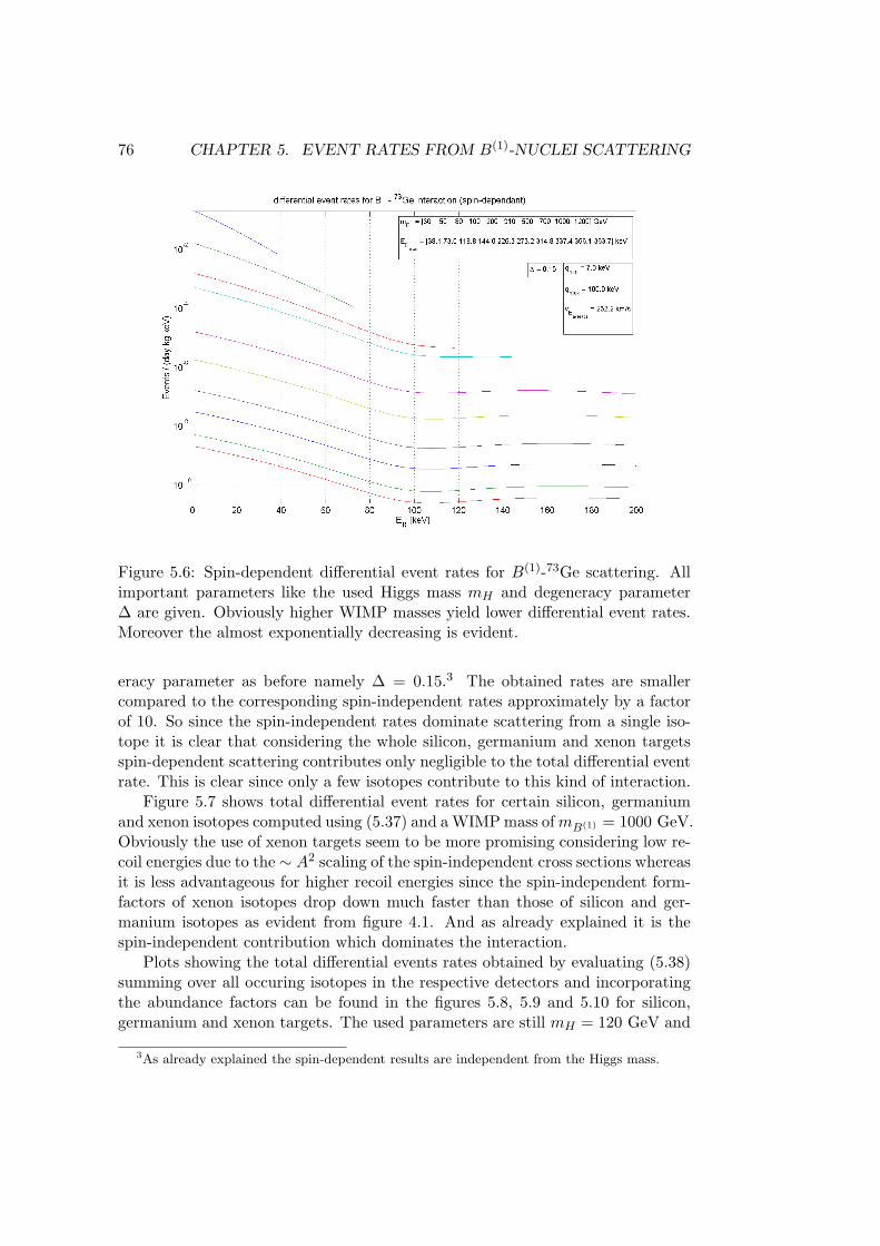
76 CHAPTER 5. EVENT RATES FROM B(1)-NUCLEI SCATTERING
Figure 5.6: Spin-dependent differential event rates for B(1)-73Ge scattering. Allimportant parameters like the used Higgs mass mH and degeneracy parameter∆ are given. Obviously higher WIMP masses yield lower differential event rates.Moreover the almost exponentially decreasing is evident.
eracy parameter as before namely ∆ = 0.15.3 The obtained rates are smallercompared to the corresponding spin-independent rates approximately by a factorof 10. So since the spin-independent rates dominate scattering from a single iso-tope it is clear that considering the whole silicon, germanium and xenon targetsspin-dependent scattering contributes only negligible to the total differential eventrate. This is clear since only a few isotopes contribute to this kind of interaction.
Figure 5.7 shows total differential event rates for certain silicon, germaniumand xenon isotopes computed using (5.37) and a WIMP mass ofmB(1) = 1000 GeV.Obviously the use of xenon targets seem to be more promising considering low re-coil energies due to the ∼ A2 scaling of the spin-independent cross sections whereasit is less advantageous for higher recoil energies since the spin-independent form-factors of xenon isotopes drop down much faster than those of silicon and ger-manium isotopes as evident from figure 4.1. And as already explained it is thespin-independent contribution which dominates the interaction.
Plots showing the total differential events rates obtained by evaluating (5.38)summing over all occuring isotopes in the respective detectors and incorporatingthe abundance factors can be found in the figures 5.8, 5.9 and 5.10 for silicon,germanium and xenon targets. The used parameters are still mH = 120 GeV and
3As already explained the spin-dependent results are independent from the Higgs mass.
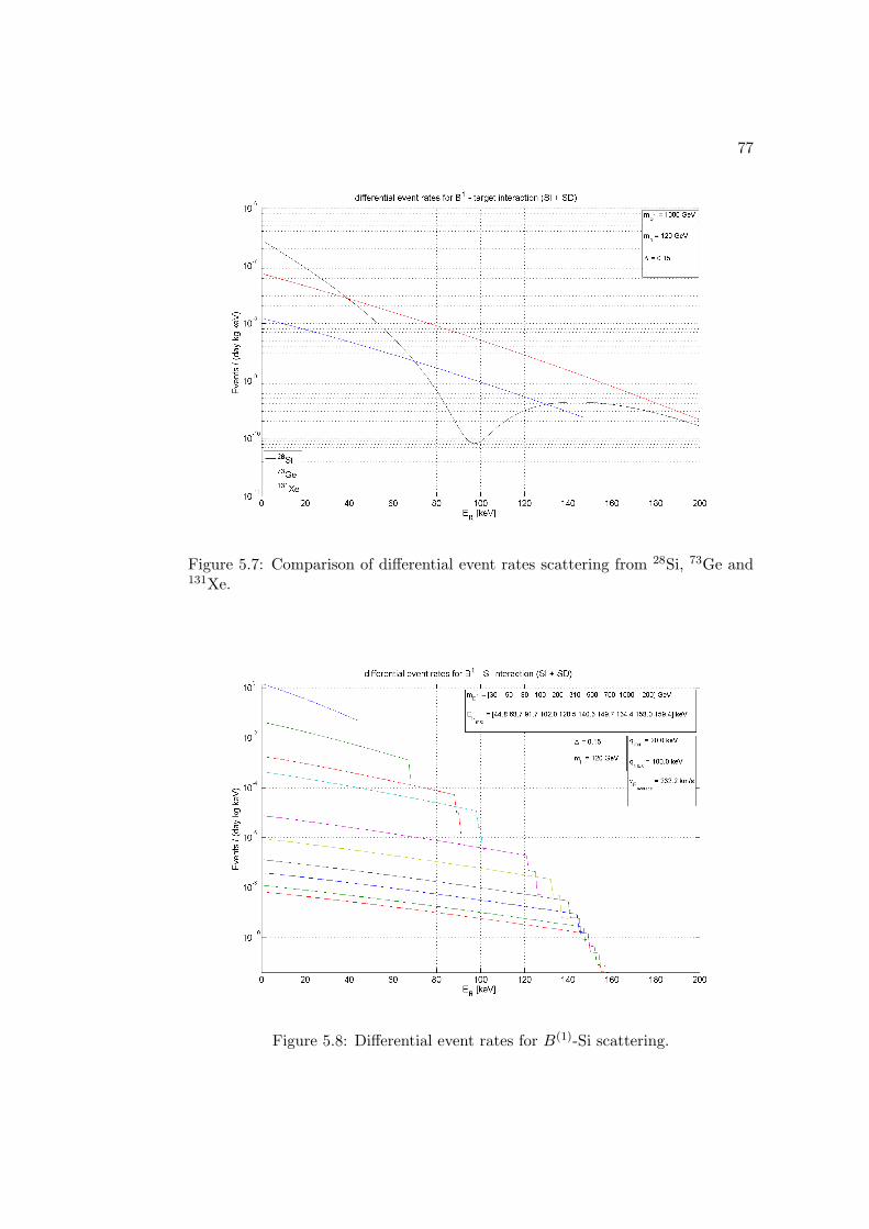
77
Figure 5.7: Comparison of differential event rates scattering from 28Si, 73Ge and131Xe.
Figure 5.8: Differential event rates for B(1)-Si scattering.
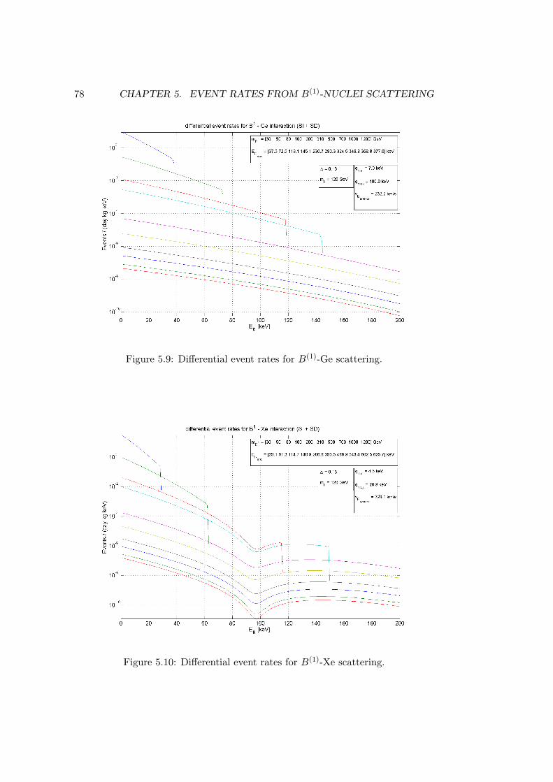
78 CHAPTER 5. EVENT RATES FROM B(1)-NUCLEI SCATTERING
Figure 5.9: Differential event rates for B(1)-Ge scattering.
Figure 5.10: Differential event rates for B(1)-Xe scattering.
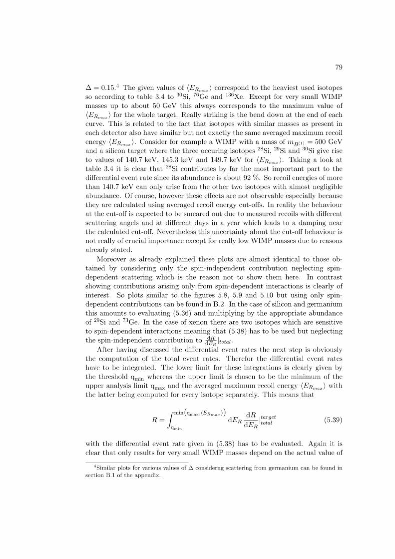
79
∆ = 0.15.4 The given values of 〈ERmax〉 correspond to the heaviest used isotopesso according to table 3.4 to 30Si, 76Ge and 136Xe. Except for very small WIMPmasses up to about 50 GeV this always corresponds to the maximum value of〈ERmax〉 for the whole target. Really striking is the bend down at the end of eachcurve. This is related to the fact that isotopes with similar masses as present ineach detector also have similar but not exactly the same averaged maximum recoilenergy 〈ERmax〉. Consider for example a WIMP with a mass of mB(1) = 500 GeVand a silicon target where the three occuring isotopes 28Si, 29Si and 30Si give riseto values of 140.7 keV, 145.3 keV and 149.7 keV for 〈ERmax〉. Taking a look attable 3.4 it is clear that 28Si contributes by far the most important part to thedifferential event rate since its abundance is about 92 %. So recoil energies of morethan 140.7 keV can only arise from the other two isotopes with almost negligibleabundance. Of course, however these effects are not observable especially becausethey are calculated using averaged recoil energy cut-offs. In reality the behaviourat the cut-off is expected to be smeared out due to measured recoils with differentscattering angels and at different days in a year which leads to a damping nearthe calculated cut-off. Nevertheless this uncertainty about the cut-off behaviour isnot really of crucial importance except for really low WIMP masses due to reasonsalready stated.
Moreover as already explained these plots are almost identical to those ob-tained by considering only the spin-independent contribution neglecting spin-dependent scattering which is the reason not to show them here. In contrastshowing contributions arising only from spin-dependent interactions is clearly ofinterest. So plots similar to the figures 5.8, 5.9 and 5.10 but using only spin-dependent contributions can be found in B.2. In the case of silicon and germaniumthis amounts to evaluating (5.36) and multiplying by the appropriate abundanceof 29Si and 73Ge. In the case of xenon there are two isotopes which are sensitiveto spin-dependent interactions meaning that (5.38) has to be used but neglectingthe spin-independent contribution to dR
dER|total.
After having discussed the differential event rates the next step is obviouslythe computation of the total event rates. Therefor the differential event rateshave to be integrated. The lower limit for these integrations is clearly given bythe threshold qmin whereas the upper limit is chosen to be the minimum of theupper analysis limit qmax and the averaged maximum recoil energy 〈ERmax〉 withthe latter being computed for every isotope separately. This means that
R =∫ min
(qmax,〈ERmax 〉
)qmin
dERdR
dER|targettotal (5.39)
with the differential event rate given in (5.38) has to be evaluated. Again it isclear that only results for very small WIMP masses depend on the actual value of
4Similar plots for various values of ∆ considerng scattering from germanium can be found insection B.1 of the appendix.
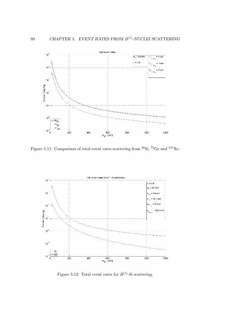
80 CHAPTER 5. EVENT RATES FROM B(1)-NUCLEI SCATTERING
Figure 5.11: Comparison of total event rates scattering from 28Si, 73Ge and 131Xe.
Figure 5.12: Total event rates for B(1)-Si scattering.
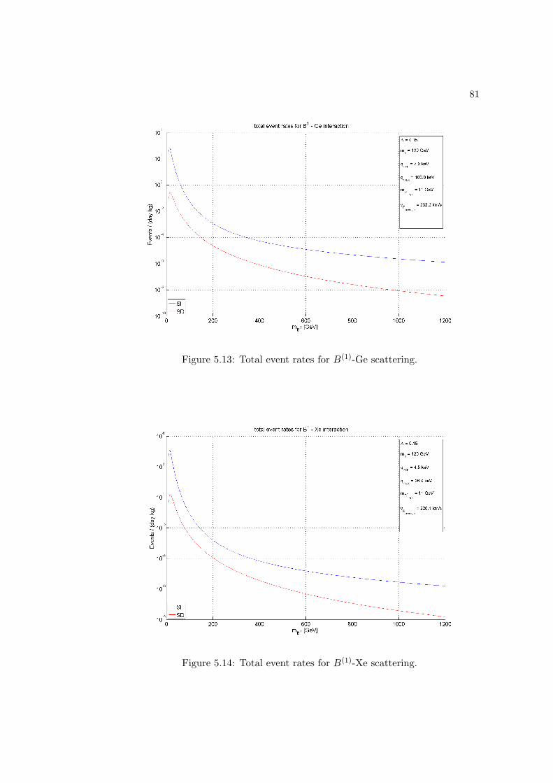
81
Figure 5.13: Total event rates for B(1)-Ge scattering.
Figure 5.14: Total event rates for B(1)-Xe scattering.
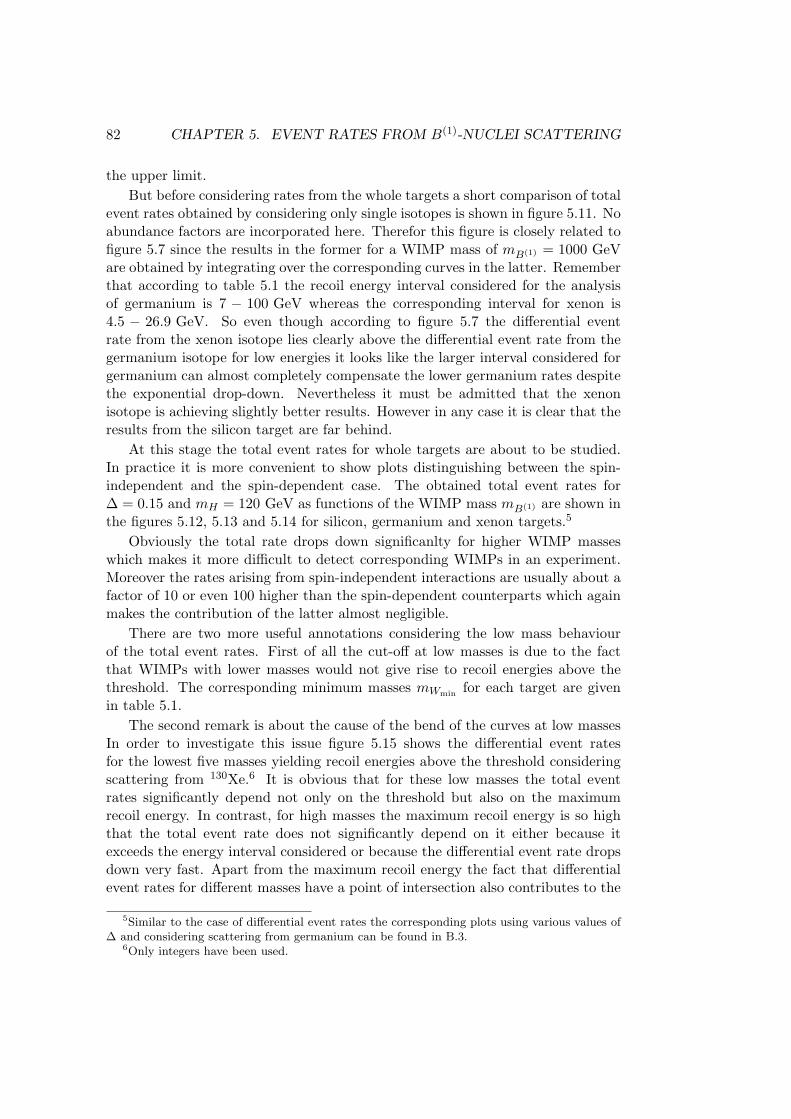
82 CHAPTER 5. EVENT RATES FROM B(1)-NUCLEI SCATTERING
the upper limit.But before considering rates from the whole targets a short comparison of total
event rates obtained by considering only single isotopes is shown in figure 5.11. Noabundance factors are incorporated here. Therefor this figure is closely related tofigure 5.7 since the results in the former for a WIMP mass of mB(1) = 1000 GeVare obtained by integrating over the corresponding curves in the latter. Rememberthat according to table 5.1 the recoil energy interval considered for the analysisof germanium is 7 − 100 GeV whereas the corresponding interval for xenon is4.5 − 26.9 GeV. So even though according to figure 5.7 the differential eventrate from the xenon isotope lies clearly above the differential event rate from thegermanium isotope for low energies it looks like the larger interval considered forgermanium can almost completely compensate the lower germanium rates despitethe exponential drop-down. Nevertheless it must be admitted that the xenonisotope is achieving slightly better results. However in any case it is clear that theresults from the silicon target are far behind.
At this stage the total event rates for whole targets are about to be studied.In practice it is more convenient to show plots distinguishing between the spin-independent and the spin-dependent case. The obtained total event rates for∆ = 0.15 and mH = 120 GeV as functions of the WIMP mass mB(1) are shown inthe figures 5.12, 5.13 and 5.14 for silicon, germanium and xenon targets.5
Obviously the total rate drops down significanlty for higher WIMP masseswhich makes it more difficult to detect corresponding WIMPs in an experiment.Moreover the rates arising from spin-independent interactions are usually about afactor of 10 or even 100 higher than the spin-dependent counterparts which againmakes the contribution of the latter almost negligible.
There are two more useful annotations considering the low mass behaviourof the total event rates. First of all the cut-off at low masses is due to the factthat WIMPs with lower masses would not give rise to recoil energies above thethreshold. The corresponding minimum masses mWmin for each target are givenin table 5.1.
The second remark is about the cause of the bend of the curves at low massesIn order to investigate this issue figure 5.15 shows the differential event ratesfor the lowest five masses yielding recoil energies above the threshold consideringscattering from 130Xe.6 It is obvious that for these low masses the total eventrates significantly depend not only on the threshold but also on the maximumrecoil energy. In contrast, for high masses the maximum recoil energy is so highthat the total event rate does not significantly depend on it either because itexceeds the energy interval considered or because the differential event rate dropsdown very fast. Apart from the maximum recoil energy the fact that differentialevent rates for different masses have a point of intersection also contributes to the
5Similar to the case of differential event rates the corresponding plots using various values of∆ and considering scattering from germanium can be found in B.3.
6Only integers have been used.

83
Figure 5.15: Differential event rates for the lowest five masses yielding recoil ener-gies above the threshold using only integers for the masses and considering scat-tering from 130Xe.
bend. For example the area under the upper blue curve between the vertical redline representing the threshold and the vertical blue line representing the averagedmaximum recoil energy for the corresponding WIMP mass is smaller than the areaunder the green curve between the vertical red and green lines. Hence the totalrate for a WIMP mass of mB(1) = 11 GeV is smaller than for a WIMP massof mB(1) = 12 GeV. As cognizable from the plot the intersection points of twoadjacent rates move to higher recoil energies for higher WIMP masses. This alsocontributes to the fact that except for low WIMP masses the total rate alwaysdecreases with increasing WIMP masses. However as already stated this bendshould not be taken too serious due to the mentioned uncertainties of the cut-offbehaviour of the differential rates. Moreover this bend disappears if a detectorhas a very low threshold close to 0 keV because then the part of the differentialevent rate directly above the threshold dominates by far. This is shown in a plotin B.4 where a threshold of 0.1 keV is assumed.
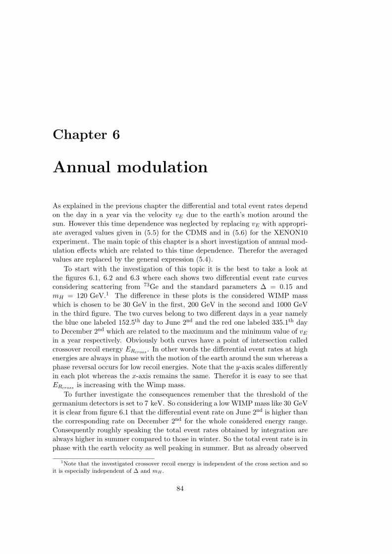
Chapter 6
Annual modulation
As explained in the previous chapter the differential and total event rates dependon the day in a year via the velocity vE due to the earth’s motion around thesun. However this time dependence was neglected by replacing vE with appropri-ate averaged values given in (5.5) for the CDMS and in (5.6) for the XENON10experiment. The main topic of this chapter is a short investigation of annual mod-ulation effects which are related to this time dependence. Therefor the averagedvalues are replaced by the general expression (5.4).
To start with the investigation of this topic it is the best to take a look atthe figures 6.1, 6.2 and 6.3 where each shows two differential event rate curvesconsidering scattering from 73Ge and the standard parameters ∆ = 0.15 andmH = 120 GeV.1 The difference in these plots is the considered WIMP masswhich is chosen to be 30 GeV in the first, 200 GeV in the second and 1000 GeVin the third figure. The two curves belong to two different days in a year namelythe blue one labeled 152.5th day to June 2nd and the red one labeled 335.1th dayto December 2nd which are related to the maximum and the minimum value of vEin a year respectively. Obviously both curves have a point of intersection calledcrossover recoil energy ERcross . In other words the differential event rates at highenergies are always in phase with the motion of the earth around the sun whereas aphase reversal occurs for low recoil energies. Note that the y-axis scales differentlyin each plot whereas the x-axis remains the same. Therefor it is easy to see thatERcross is increasing with the Wimp mass.
To further investigate the consequences remember that the threshold of thegermanium detectors is set to 7 keV. So considering a low WIMP mass like 30 GeVit is clear from figure 6.1 that the differential event rate on June 2nd is higher thanthe corresponding rate on December 2nd for the whole considered energy range.Consequently roughly speaking the total event rates obtained by integration arealways higher in summer compared to those in winter. So the total event rate is inphase with the earth velocity as well peaking in summer. But as already observed
1Note that the investigated crossover recoil energy is independent of the cross section and soit is especially independent of ∆ and mH .
84
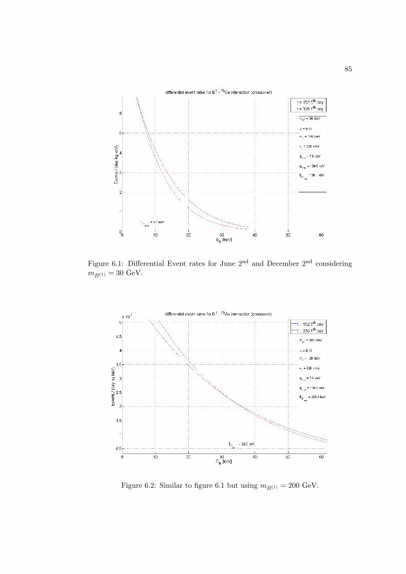
85
Figure 6.1: Differential Event rates for June 2nd and December 2nd consideringmB(1) = 30 GeV.
Figure 6.2: Similar to figure 6.1 but using mB(1) = 200 GeV.
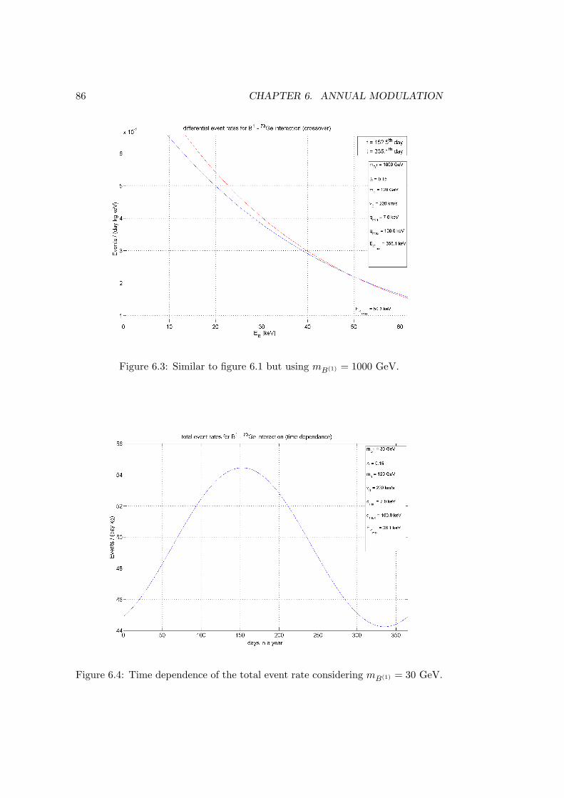
86 CHAPTER 6. ANNUAL MODULATION
Figure 6.3: Similar to figure 6.1 but using mB(1) = 1000 GeV.
Figure 6.4: Time dependence of the total event rate considering mB(1) = 30 GeV.
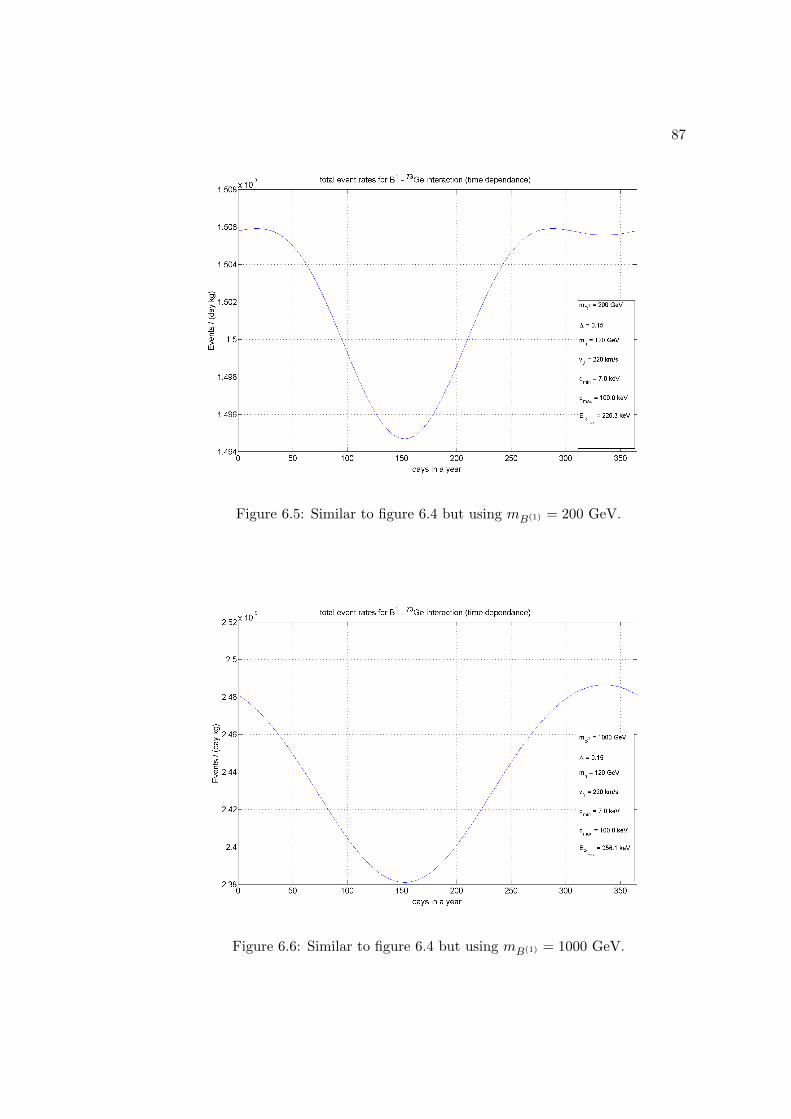
87
Figure 6.5: Similar to figure 6.4 but using mB(1) = 200 GeV.
Figure 6.6: Similar to figure 6.4 but using mB(1) = 1000 GeV.
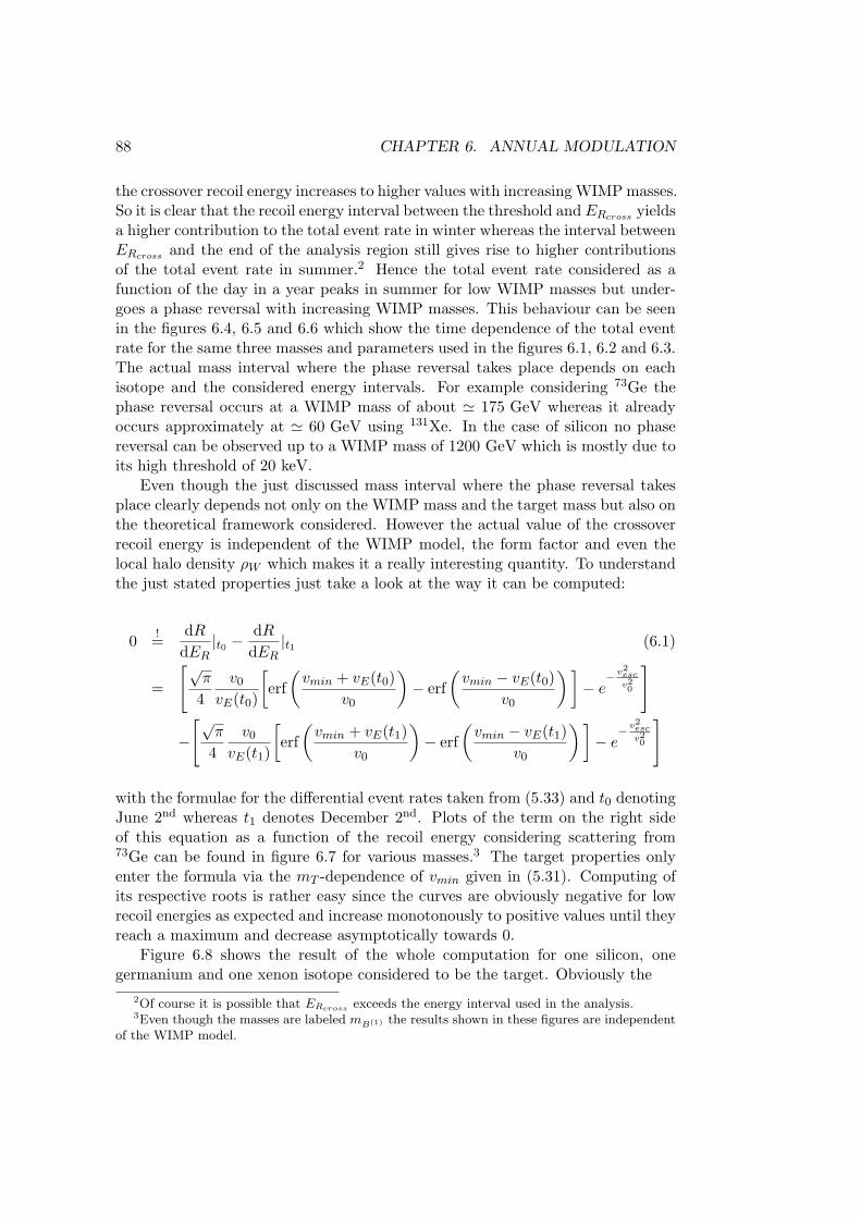
88 CHAPTER 6. ANNUAL MODULATION
the crossover recoil energy increases to higher values with increasing WIMP masses.So it is clear that the recoil energy interval between the threshold and ERcross yieldsa higher contribution to the total event rate in winter whereas the interval betweenERcross and the end of the analysis region still gives rise to higher contributionsof the total event rate in summer.2 Hence the total event rate considered as afunction of the day in a year peaks in summer for low WIMP masses but under-goes a phase reversal with increasing WIMP masses. This behaviour can be seenin the figures 6.4, 6.5 and 6.6 which show the time dependence of the total eventrate for the same three masses and parameters used in the figures 6.1, 6.2 and 6.3.The actual mass interval where the phase reversal takes place depends on eachisotope and the considered energy intervals. For example considering 73Ge thephase reversal occurs at a WIMP mass of about ' 175 GeV whereas it alreadyoccurs approximately at ' 60 GeV using 131Xe. In the case of silicon no phasereversal can be observed up to a WIMP mass of 1200 GeV which is mostly due toits high threshold of 20 keV.
Even though the just discussed mass interval where the phase reversal takesplace clearly depends not only on the WIMP mass and the target mass but also onthe theoretical framework considered. However the actual value of the crossoverrecoil energy is independent of the WIMP model, the form factor and even thelocal halo density ρW which makes it a really interesting quantity. To understandthe just stated properties just take a look at the way it can be computed:
0 !=dR
dER|t0 −
dRdER
|t1 (6.1)
=
[√π
4v0
vE(t0)
[erf(vmin + vE(t0)
v0
)− erf
(vmin − vE(t0)
v0
)]− e− v
2escv20
]
−
[√π
4v0
vE(t1)
[erf(vmin + vE(t1)
v0
)− erf
(vmin − vE(t1)
v0
)]− e− v
2escv20
]
with the formulae for the differential event rates taken from (5.33) and t0 denotingJune 2nd whereas t1 denotes December 2nd. Plots of the term on the right sideof this equation as a function of the recoil energy considering scattering from73Ge can be found in figure 6.7 for various masses.3 The target properties onlyenter the formula via the mT -dependence of vmin given in (5.31). Computing ofits respective roots is rather easy since the curves are obviously negative for lowrecoil energies as expected and increase monotonously to positive values until theyreach a maximum and decrease asymptotically towards 0.
Figure 6.8 shows the result of the whole computation for one silicon, onegermanium and one xenon isotope considered to be the target. Obviously the
2Of course it is possible that ERcross exceeds the energy interval used in the analysis.3Even though the masses are labeled mB(1) the results shown in these figures are independent
of the WIMP model.
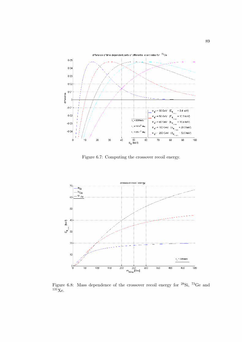
89
Figure 6.7: Computing the crossover recoil energy.
Figure 6.8: Mass dependence of the crossover recoil energy for 28Si, 73Ge and131Xe.
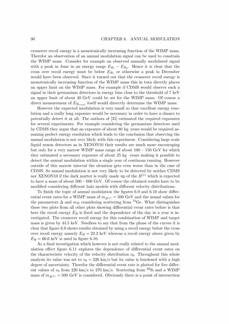
90 CHAPTER 6. ANNUAL MODULATION
crossover recoil energy is a monotonically increasing function of the WIMP mass.Therefor an observation of an annual modulation signal can be used to constrainthe WIMP mass. Consider for example an observed annually modulated signalwith a peak in June in an energy range ER1 − ER2 . Hence it is clear that thecross over recoil energy must be below ER1 or otherwise a peak in Decemberwould have been observed. Since it turned out that the crossover recoil energy ismonotonically increasing function of the WIMP mass this in turn directly placesan upper limit on the WIMP mass. For example if CDMS would observe such asignal in their germanium detectors in energy bins close to the threshold of 7 keVan upper limit of about 40 GeV could be set for the WIMP mass. Of course adirect measurement of ERcross itself would direcctly determine the WIMP mass.
However the expected modulation is very small so that excellent energy reso-lution and a really long exposure would be necessary in order to have a chance topotentially detect it at all. The authors of [35] estimated the required exposuresfor several experiments. For example considering the germanium detectors usedby CDMS they argue that an exposure of about 80 kg ·years would be required as-suming perfect energy resolution which leads to the conclusion that observing theannual modulation is not very likely with this experiment. Considering large scaleliquid xenon detectors as in XENON10 their results are much more encouragingbut only for a very narrow WIMP mass range of about 100− 150 GeV for whichthey estimated a necessary exposure of about 25 kg · years making it possible todetect the annual modulation within a single year of continous running. Howeveroutside of this narrow interval the situation gets even worse than in the case ofCDMS. So annual modulation is not very likely to be detected by neither CDMSnor XENON10 if the dark matter is really made up of the B(1) which is expectedto have a mass of about 500−600 GeV. Of course the obtained results have to bemodified considering different halo models with different velocity distributions.
To finish the topic of annual modulation the figures 6.9 and 6.10 show differ-ential event rates for a WIMP mass of mB(1) = 500 GeV and the ususal values forthe parameters ∆ and mH considering scattering from 73Ge. What distinguishesthese two plots from all other plots showing differential event rates before is thathere the recoil energy ER is fixed and the dependence of the day in a year is in-vestigated. The crossover recoil energy for this combination of WIMP and targetmass is given by 44.5 keV. Needless to say that from the phase of the curves it isclear that figure 6.9 shows results obtained by using a recoil energy below the crossover recoil energy namely ER = 22.2 keV whereas a recoil energy above given byER = 66.6 keV is used in figure 6.10.
As a final investigation which however is not really related to the annual mod-ulation effect figure 6.11 explores the dependence of differential event rates onthe characteristic velocity of the velocity distribution v0. Throughout this wholeanalysis its value was set to v0 = 220 km/s but its value is burdened with a highdegree of uncertainty. Therefor the differential event rate is plotted for five differ-ent values of v0 from 220 km/s to 270 km/s. Scattering from 29Si and a WIMPmass of mB(1) = 500 GeV is considered. Obviously there is a point of intersection
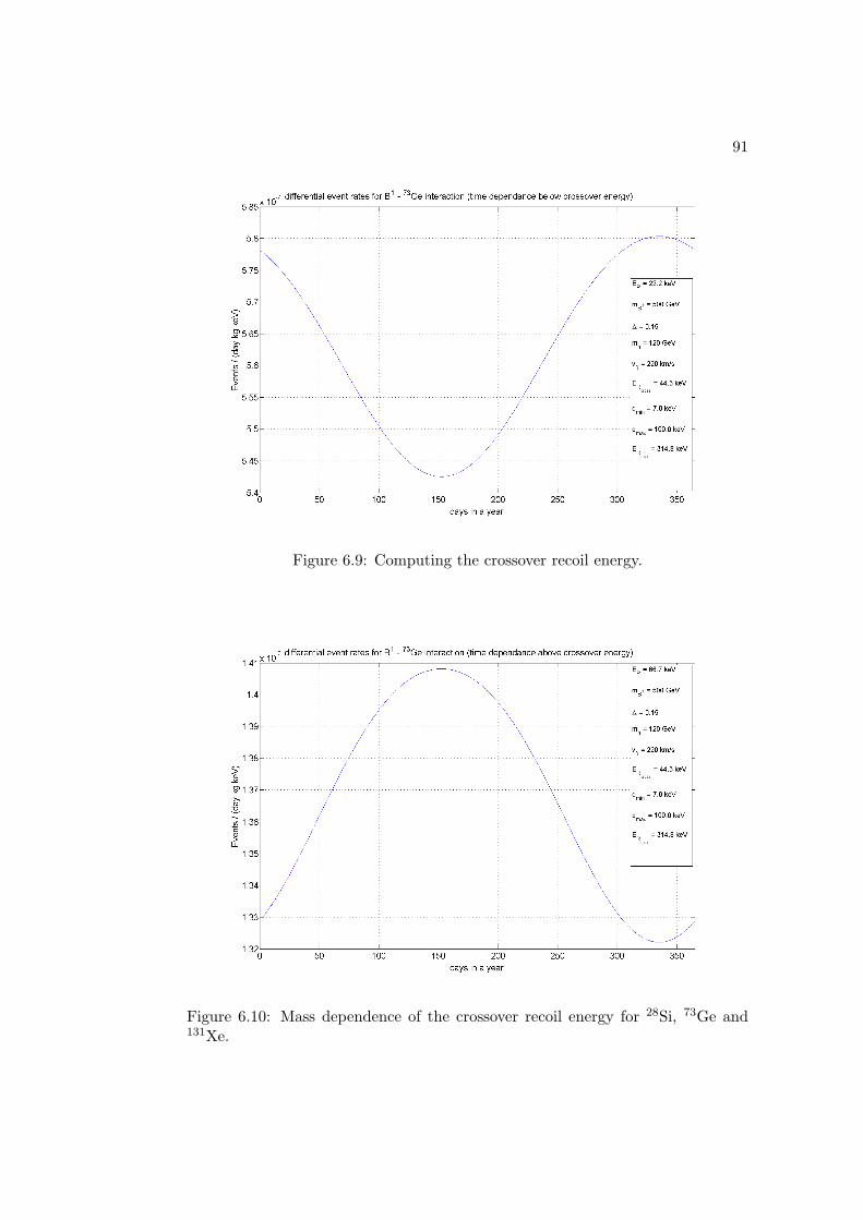
91
Figure 6.9: Computing the crossover recoil energy.
Figure 6.10: Mass dependence of the crossover recoil energy for 28Si, 73Ge and131Xe.
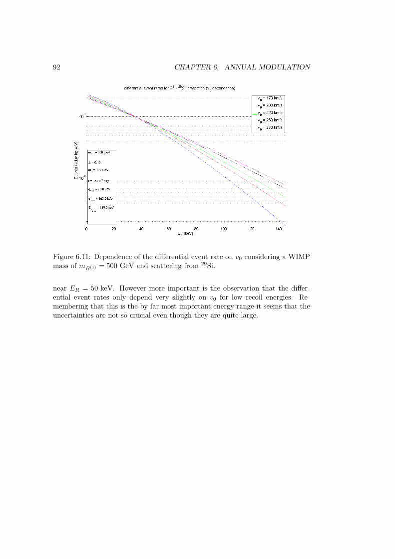
92 CHAPTER 6. ANNUAL MODULATION
Figure 6.11: Dependence of the differential event rate on v0 considering a WIMPmass of mB(1) = 500 GeV and scattering from 29Si.
near ER = 50 keV. However more important is the observation that the differ-ential event rates only depend very slightly on v0 for low recoil energies. Re-membering that this is the by far most important energy range it seems that theuncertainties are not so crucial even though they are quite large.
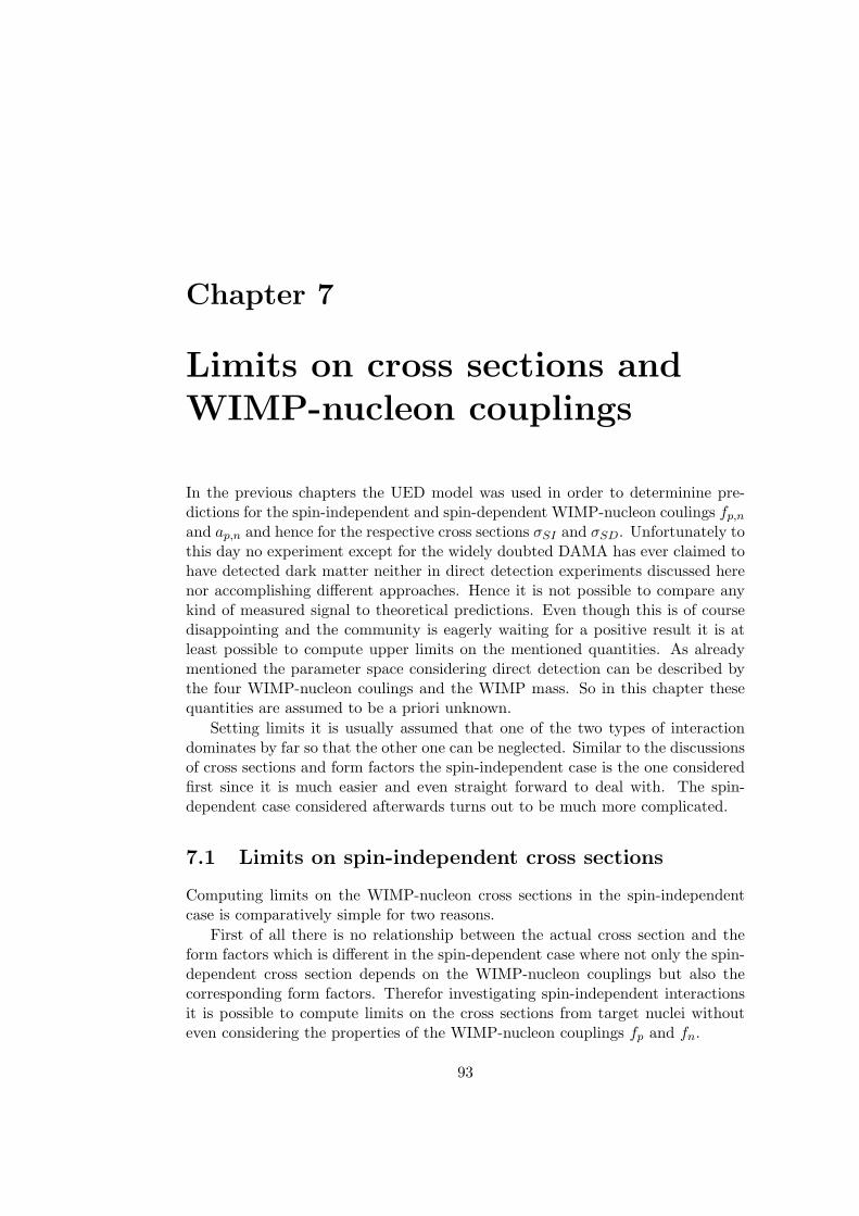
Chapter 7
Limits on cross sections andWIMP-nucleon couplings
In the previous chapters the UED model was used in order to determinine pre-dictions for the spin-independent and spin-dependent WIMP-nucleon coulings fp,nand ap,n and hence for the respective cross sections σSI and σSD. Unfortunately tothis day no experiment except for the widely doubted DAMA has ever claimed tohave detected dark matter neither in direct detection experiments discussed herenor accomplishing different approaches. Hence it is not possible to compare anykind of measured signal to theoretical predictions. Even though this is of coursedisappointing and the community is eagerly waiting for a positive result it is atleast possible to compute upper limits on the mentioned quantities. As alreadymentioned the parameter space considering direct detection can be described bythe four WIMP-nucleon coulings and the WIMP mass. So in this chapter thesequantities are assumed to be a priori unknown.
Setting limits it is usually assumed that one of the two types of interactiondominates by far so that the other one can be neglected. Similar to the discussionsof cross sections and form factors the spin-independent case is the one consideredfirst since it is much easier and even straight forward to deal with. The spin-dependent case considered afterwards turns out to be much more complicated.
7.1 Limits on spin-independent cross sections
Computing limits on the WIMP-nucleon cross sections in the spin-independentcase is comparatively simple for two reasons.
First of all there is no relationship between the actual cross section and theform factors which is different in the spin-dependent case where not only the spin-dependent cross section depends on the WIMP-nucleon couplings but also thecorresponding form factors. Therefor investigating spin-independent interactionsit is possible to compute limits on the cross sections from target nuclei withouteven considering the properties of the WIMP-nucleon couplings fp and fn.
93
94CHAPTER 7. LIMITS ON CROSS SECTIONS AND WIMP-NUCLEON COUPLINGS
The second reason concerns the normalization from cross section limits con-sidering target nuclei to the limits from scattering of single nucleons. As alreadymentioned in the chapter on cross sections it is appropriate for most dark mat-ter candidates to assume that the interaction is isospin-independent which meansthat fp ≈ fn yielding the simple normalization given in (3.19). Even though thisnormalization is used throughout this whole chapter it is useful to think aboutthe consequences if the just made assumption does not hold. This is discussed forexample in [36]. Consider for example the extreme case that fp = −fn. From (3.9)it is clear that this would result in a strongly suppression of the spin-independentinteraction with the advantegeous ∼ A2 scaling from the isospin-independent caseswitching to a ∼ (N−Z)2 scaling. Of course this would be disastrous especially forexperiments with comparatively low target masses where N ≈ Z. So taking a lookat table 3.4 reveals that for example 73Ge would end up with only 9 nucleons effec-tively participating in the interaction whereas 131Xe would still constitute at least23 effective nucleons. Hence the sensitivity of these targets would be suppressed byfactors of approximately 66 and 32 respectively. For the general case of arbitraryWIMP-nucleon couplings an analysis similar to the approach presented for spin-dependent interactions constraining fp and fn would be necessary which howeverwould be still less complicated due to the almost target-independent form factors.Nevertheless as already mentioned the simple case assuming isospin-independentinteractions is investigated here.
So how are cross section limits computed? In order to answer this questionthe arrangement is made to start by calculating limits for every target isotopeseperately and combining them afterwards. The general procedure is rather sim-ple. First of all the number of events N has to be considered. It can be calculatedby multiplying the total event rate with the respective abundance factor f givenin table 3.4 as well as the exposure exp and efficiency eff given in table 5.1. Sousing the expression for the spin-independent differential event rate consideringscattering from only one single isotope given in (5.35) and directly replacing σSIby the cross section normalized to a neutron given in (3.19) yields1
N = f · exp · eff · σnSI A2 µ2T
µ2n
∫ min(
qmax,〈ERmax 〉)
qmin
dRdER
|σ F 2SI dER . (7.1)
All factors in front of the integral are clearly independent of the recoil energy.However in the general case the efficiency is also energy dependent which has tobe taken into account. (7.1) directly yields an expression for the cross section. Nclearly has to be estimated by analyzing data from the respective experiments.After this is done the corresponding normalized cross section can be computedusing
1Of course normalizing to scattering from a proton would yield almost exactly the same results.
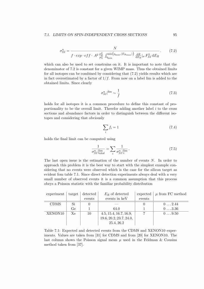
7.1. LIMITS ON SPIN-INDEPENDENT CROSS SECTIONS 95
σnSI =N
f · exp · eff · A2 µ2Tµ2n
∫ min(
qmax,〈ERmax 〉)
qmin
dRdER|σ F 2
SI dER. (7.2)
which can also be used to set constrains on it. It is important to note that thedenominator of 7.2 is constant for a given WIMP mass. Thus the obtained limitsfor all isotopes can be combined by considering that (7.2) yields results which arein fact overestimated by a factor of 1/f . From now on a label lim is added to theobtained limits. Since clearly
σnSI |lim ∼1f
(7.3)
holds for all isotopes it is a common procedure to define this constant of pro-portionality to be the overall limit. Therefor adding another label i to the crosssections and abundance factors in order to distinguish between the different iso-topes and considering that obviously∑
i
fi = 1 (7.4)
holds the final limit can be computed using
1σnSI |limtotal
=∑i
1σnSI |limi
. (7.5)
The last open issue is the estimation of the number of events N . In order toapproach this problem it is the best way to start with the simplest example con-sidering that no events were observed which is the case for the silicon target asevident fom table 7.1. Since direct detection experiments always deal with a verysmall number of observed events it is a common assumption that this processobeys a Poisson statistic with the familiar probability distribution
experiment target detected ER of detected expected µ from FC methodevents events in keV events
CDMS Si 0 — 0 0 . . . 2.44Ge 1 64.0 1 0 . . . 3.36
XENON10 Xe 10 4.5, 15.4, 16.7, 16.9, 7 0 . . . 9.5019.6, 20.2, 23.7, 24.0,
25.4, 26.2
Table 7.1: Expected and detected events from the CDMS and XENON10 exper-iments. Values are taken from [31] for CDMS and from [20] for XENON10. Thelast column shows the Poisson signal mean µ used in the Feldman & Cousinsmethod taken from [37].
96CHAPTER 7. LIMITS ON CROSS SECTIONS AND WIMP-NUCLEON COUPLINGS
P (k|µ) =µk
k!e−µ (7.6)
where µ denotes the expectation value. Usually a 90 % confidence limit is givenon the cross sections. In the case that no events were observed or rather k = 0this is easily evaluated.
P (0|λ) = e−µ!= 1− 0.9 (7.7)
directly yields µ = ln 10 ≈ 2.30 which henceforth is used as the number of eventsN in (7.2). To summarize this procedure using N = ln 10 in (7.2) yields a 90 %upper confidence limit on the cross section.
Nevertheless usually a small number of events is detected and moreover es-timations on the occuring background should be included in the computationsif possible. Therefor more advanced analysis techniques are necessary. In thefollowing two different approaches are investigated which are called the Feld-man & Cousins method presented in [37] and the Maximum Gap method fromSteve Yellin published in [38].
The Feldman & Cousins method is distinguished from other classical ap-proaches of setting limits especially by the fact that the decision whether upperlimits or two-sided confidence intervals should be computed is not made by theperson doing the analysis but rather intrinsically by the procedure itself. This isvery promising because the authors of [37] showed that the obtained limits are notreally confidence intervals if the choice is based on the data obtained. Moreoverthis method avoids the possible occurance of unphysical or empty intervals. Inorder to briefly explain the method consider a Poisson process with an unknownexpectation value µ and a background with known mean b
P (k|µ) =(µ+ b)k
k!e−(µ+b) . (7.8)
The used procedure amounts to the accomplishment of a certain ordering principle.So considering the fixed background b and a fixed value of µ the correspondingpropability (7.8) is computed for several observed events k starting from k = 0.Hence the ratio
R =P (k|µ)
P (k|µbest)(7.9)
is computed for all k with P (k|µbest) denoting the use of that value of µ whichgives rise to the maximum possible value of P (k|µ). This parameter R defines theordering principle. So the value of n with the highest corresponding value of R isthe first value put into the acceptance region. Thus values of n are added to this
7.1. LIMITS ON SPIN-INDEPENDENT CROSS SECTIONS 97
region in decreasing order of R until the sum of P (k|µ) finally meets or exceedsthe considered confidence level which is 90 % in this case.
Fortunatelly the authors were so kind to provide some tables with preparedresults for certain confidence levels including 90 %. Therefor having observed acertain number of events and estimated the number of expected background eventsthe only thing to do is take a look at these tables and find the already computedconfidence level for the signal mean µ. The results considering the CDMS andXENON10 experiments can be found in table 7.1. Obviously it turns out thatall limits are upper limits and not central confidence intervals as it was expected.Hence the given upper values have to be inserted into (7.2) so for exampleN = 2.44for silicon. So the modification in the case where the pure Poisson approach isvalid as well since no events are detected the Feldman & Cousins method amountsto replace N = 2.30 by N = 2.44. A disadvantage of this method is that itonly incorporates the pure number of events and not their energy distribution.Moreover apart from the normalization even the expected shape of the event dis-tribution is known. The Maximum Gap method incorporates these informationfinally yielding more stringent limits.
The Maximum Gap method can be used to compute cross section limits ina slightly different way. Unlike the Feldman & Cousins method it is also ap-plicable if there is a certain unknown background contaminating the data. Thebasic procedure is to find a certain energy range yielding an especially stringentlimit. Therefor an interval has to be chosen where the sum of the signal and thebackground is particularly small. However this is not done manually which wouldbe very subjective since for example low energy ranges are usually dominated bybackground signals which would result in a weaker upper limit but included in theprocedure. It works as follows:
The unbinned data is considered and for every interval between two adjacentmeasured events the expected number of events is computed which is clearly givenby (7.1) but with the the integration limits replaced by the recoil energies of thesetwo events. Since the cross section is unknown this means that the right side ofthe equation without considering σnSI has to be evaluated. Of course the upperand lower analysis limits serve as integration limits as well. So for example takinga look at the germanium data given in table 7.1 it is clear that two intervals haveto be considered namely 7−64 keV and 64−100keV. Moreover there is obviouslyonly one interval in the silicon case and eleven considering xenon. It should be self-evident that these integrations might have to be cut-off at the averaged maximumrecoil energy. After executing all these computations the one with the highestresulting number of expected events labeled x is chosen which defines the so-called Maximum Gap. It is this interval which is used to compute the upper limit.Remember that the actual expected number of events in the Maximum Gap isstill not known since the obtained result still has to be multiplied with the crosssection so it would be more precise to write x(σnSI). However the author of [38]derived a formula for the propability C0 that the maximum gap is smaller than acertain value of x. It is only dependent on x and µ with the latter clearly being
98CHAPTER 7. LIMITS ON CROSS SECTIONS AND WIMP-NUCLEON COUPLINGS
obtained by integrating over the whole energy range:
C0(x, µ) =m∑k=0
=(kx− µ)k−1e−kx
k!
(k(x− 1)− µ
)(7.10)
m denotes the greatest integer ≤ µx . Therefor a 90 % confidence level can be
obtained increasing σnSI until C0 = 0.9. An interesting case occurs when no eventsare detected so for example considering the silicon detectors. Then x = µ givesrise to
C0(µ, µ) = 1− eµ . (7.11)
Demanding C0 = 0.9 directly yields µ = ln 10 ≈ 2.30 which is nothing but thepure Poisson limit. This has been used to check the correctness of the MaximumGap code.
To summarize some of the properties of this method it is clear that it is notvery sensitive to the boundaries of the whole energy range considered. Moreoverit does not use any kind of binning. Besides it uses information about the shapeof the event distribution and it is possible to include unknown background whichis different from the Feldman & Cousins method which only incorporates theactual number of events and requires information about the expected background.Therefor the obtained results are usually more stringent. Finally it is importantto know that this method is excellent to compute upper limits but it cannot beused to analyze a positive WIMP search signal.
As an annotation the author also published a generalization of the MaximumGap method in the same paper called Optimum Interval method. This procedureis similar to the Maximum Gap method however not only empty intervals are con-sidered but intervals with an arbitrary number of events. For example in the caseof germanium there are three different intervals namely the two already mentioned7 − 64 keV and 64 − 100 keV containing no event at all and the whole analysisrange from 7− 100 keV containing one event. Unfortunately these investigationsdo not yield an analytic formula to compute a limit similar to (7.10). InsteadMonte Carlo methods are needed to evaluate occuring functions. Fortunately re-sulting tables and several routines are published on the internet [39]. This methodwas used to compute spin-independent cross section limits as well. The resultscan be found in C.1. However since they totally agree with the results obtainedusing the Maximum Gap method considering silicon and germanium only the lat-ter is accomplished in the spin-dependent case described in the next chapter. Thereason for the bend around 50 GeV using xenon is unfortunately not known.
Finally the results of the computations for each target after using (7.5) includ-ing the Feldman & Cousins method as well as the Maxmum Gap method can befound in the figures 7.1, 7.2 and 7.3. Since the ansatz for the cross section (3.9) ismodel-independent these limits are clearly model-independent as well. However
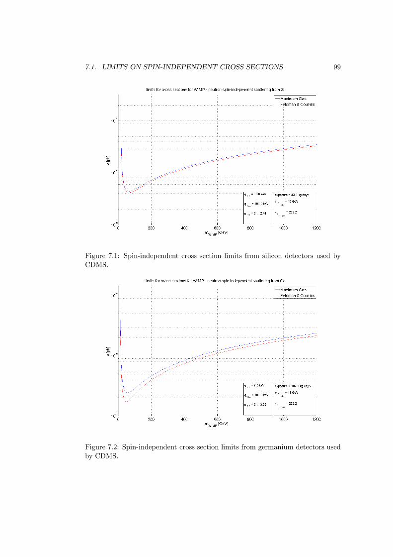
7.1. LIMITS ON SPIN-INDEPENDENT CROSS SECTIONS 99
Figure 7.1: Spin-independent cross section limits from silicon detectors used byCDMS.
Figure 7.2: Spin-independent cross section limits from germanium detectors usedby CDMS.
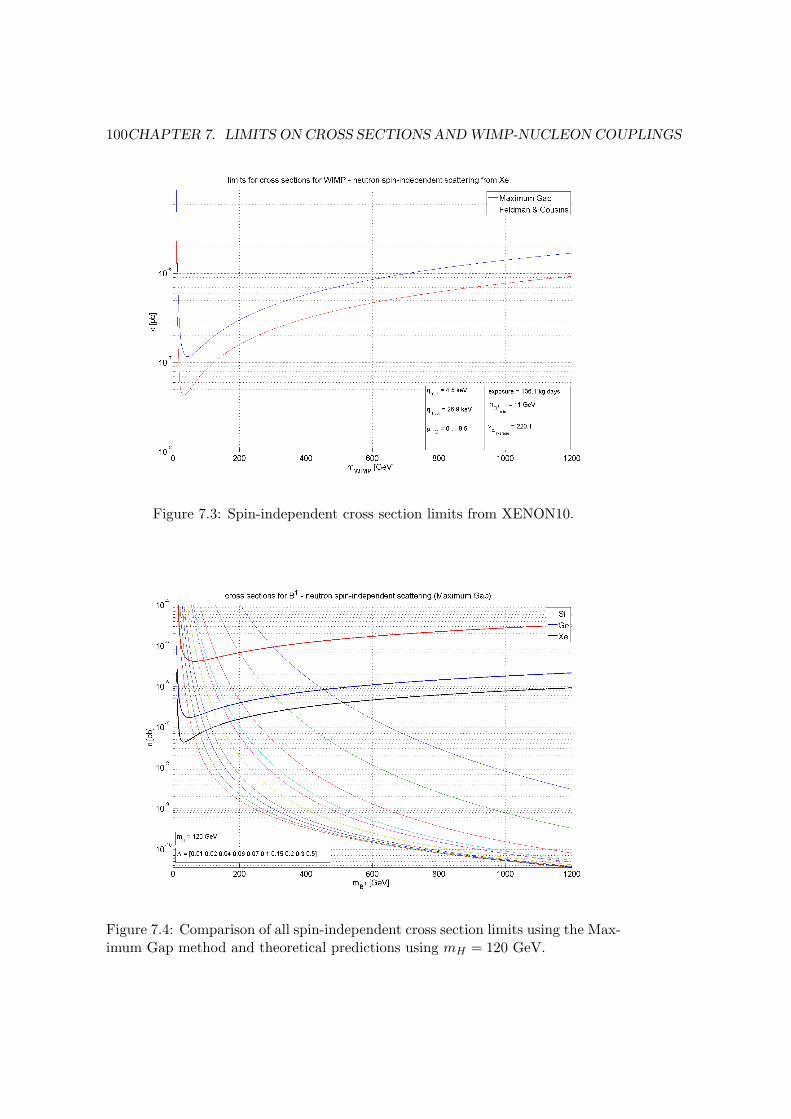
100CHAPTER 7. LIMITS ON CROSS SECTIONS AND WIMP-NUCLEON COUPLINGS
Figure 7.3: Spin-independent cross section limits from XENON10.
Figure 7.4: Comparison of all spin-independent cross section limits using the Max-imum Gap method and theoretical predictions using mH = 120 GeV.
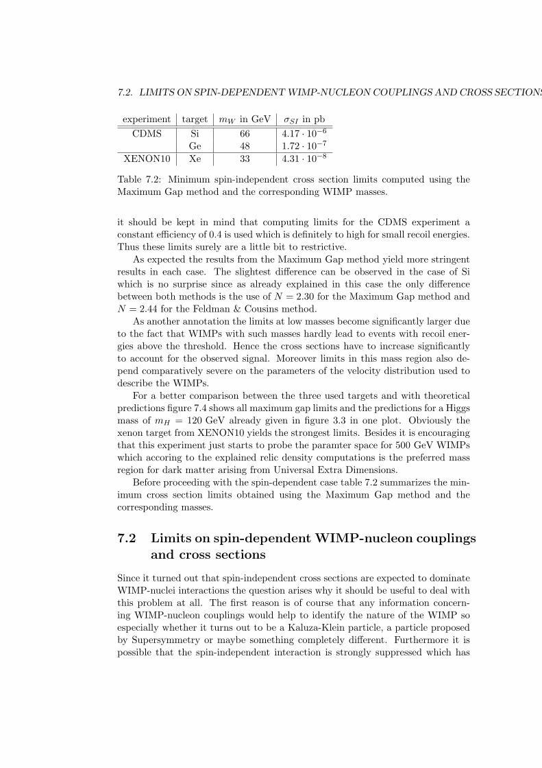
7.2. LIMITS ON SPIN-DEPENDENT WIMP-NUCLEON COUPLINGS AND CROSS SECTIONS101
experiment target mW in GeV σSI in pbCDMS Si 66 4.17 · 10−6
Ge 48 1.72 · 10−7
XENON10 Xe 33 4.31 · 10−8
Table 7.2: Minimum spin-independent cross section limits computed using theMaximum Gap method and the corresponding WIMP masses.
it should be kept in mind that computing limits for the CDMS experiment aconstant efficiency of 0.4 is used which is definitely to high for small recoil energies.Thus these limits surely are a little bit to restrictive.
As expected the results from the Maximum Gap method yield more stringentresults in each case. The slightest difference can be observed in the case of Siwhich is no surprise since as already explained in this case the only differencebetween both methods is the use of N = 2.30 for the Maximum Gap method andN = 2.44 for the Feldman & Cousins method.
As another annotation the limits at low masses become significantly larger dueto the fact that WIMPs with such masses hardly lead to events with recoil ener-gies above the threshold. Hence the cross sections have to increase significantlyto account for the observed signal. Moreover limits in this mass region also de-pend comparatively severe on the parameters of the velocity distribution used todescribe the WIMPs.
For a better comparison between the three used targets and with theoreticalpredictions figure 7.4 shows all maximum gap limits and the predictions for a Higgsmass of mH = 120 GeV already given in figure 3.3 in one plot. Obviously thexenon target from XENON10 yields the strongest limits. Besides it is encouragingthat this experiment just starts to probe the paramter space for 500 GeV WIMPswhich accoring to the explained relic density computations is the preferred massregion for dark matter arising from Universal Extra Dimensions.
Before proceeding with the spin-dependent case table 7.2 summarizes the min-imum cross section limits obtained using the Maximum Gap method and thecorresponding masses.
7.2 Limits on spin-dependent WIMP-nucleon couplingsand cross sections
Since it turned out that spin-independent cross sections are expected to dominateWIMP-nuclei interactions the question arises why it should be useful to deal withthis problem at all. The first reason is of course that any information concern-ing WIMP-nucleon couplings would help to identify the nature of the WIMP soespecially whether it turns out to be a Kaluza-Klein particle, a particle proposedby Supersymmetry or maybe something completely different. Furthermore it ispossible that the spin-independent interaction is strongly suppressed which has
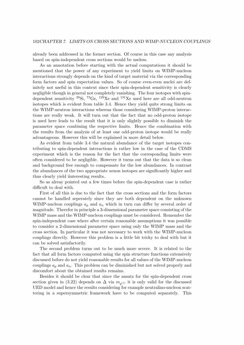
102CHAPTER 7. LIMITS ON CROSS SECTIONS AND WIMP-NUCLEON COUPLINGS
already been addressed in the former section. Of course in this case any analysisbased on spin-independent cross sections would be useless.
As an annotation before starting with the actual computations it should bementioned that the power of any experiment to yield limits on WIMP-nucleoninteractions strongly depends on the kind of target material via the correspondingform factors and spin expectation values. So of course even-even nuclei are def-initely not useful in this context since their spin-dependent sensitivity is clearlynegligible though in general not completely vanishing. The four isotopes with spin-dependent sensitivity 29Si, 73Ge, 129Xe and 131Xe used here are all odd-neutronisotopes which is evident from table 3.4. Hence they yield quite strong limits onthe WIMP-neutron interactions whereas those considering WIMP-proton interac-tions are really weak. It will turn out that the fact that no odd-proton isotopeis used here leads to the result that it is only slightly possible to diminish theparameter space combining the respective limits. Hence the combination withthe results from the analysis of at least one odd-proton isotope would be reallyadvantageous. However this will be explained in more detail below.
As evident from table 3.4 the natural abundance of the target isotopes con-tributing to spin-dependent interactions is rather low in the case of the CDMSexperiment which is the reason for the fact that the corresponding limits wereoften considered to be negligible. However it turns out that the data is so cleanand background free enough to compensate for the low abundances. In contrastthe abundances of the two appropriate xenon isotopes are significantly higher andthus clearly yield iinteresting results..
So as alreay pointed out a few times before the spin-dependent case is ratherdifficult to deal with.
First of all this is due to the fact that the cross sections and the form factorscannot be handled seperately since they are both dependent on the unknownWIMP-nucleon couplings ap and an which in turn can differ by several order ofmagnitude. Therefor in principle a 3-dimensional parameter space consisting of theWIMP mass and the WIMP-nucleon couplings must be considered. Remember thespin-independent case where after certain reasonable assumptions it was possibleto consider a 2-dimensional parameter space using only the WIMP mass and thecross section. In particular it was not necessary to work with the WIMP-nucleoncouplings directly. However this problem is a little bit tricky to deal with but itcan be solved satisfactorily.
The second problem turns out to be much more severe. It is related to thefact that all form factors computed using the spin structure functions extensivelydiscussed before do not yield reasonable results for all values of the WIMP-nucleoncouplings ap and an. This problem can be diminished but not solved properly anddiscomfort about the obtained results remains.
Besides it should be clear that since the ansatz for the spin-dependent crosssection given in (3.22) depends on ∆ via mq(1) it is only valid for the discussedUED model and hence the results considering for example neutralino-nucleon scat-tering in a supersymmetric framework have to be computed separately. This
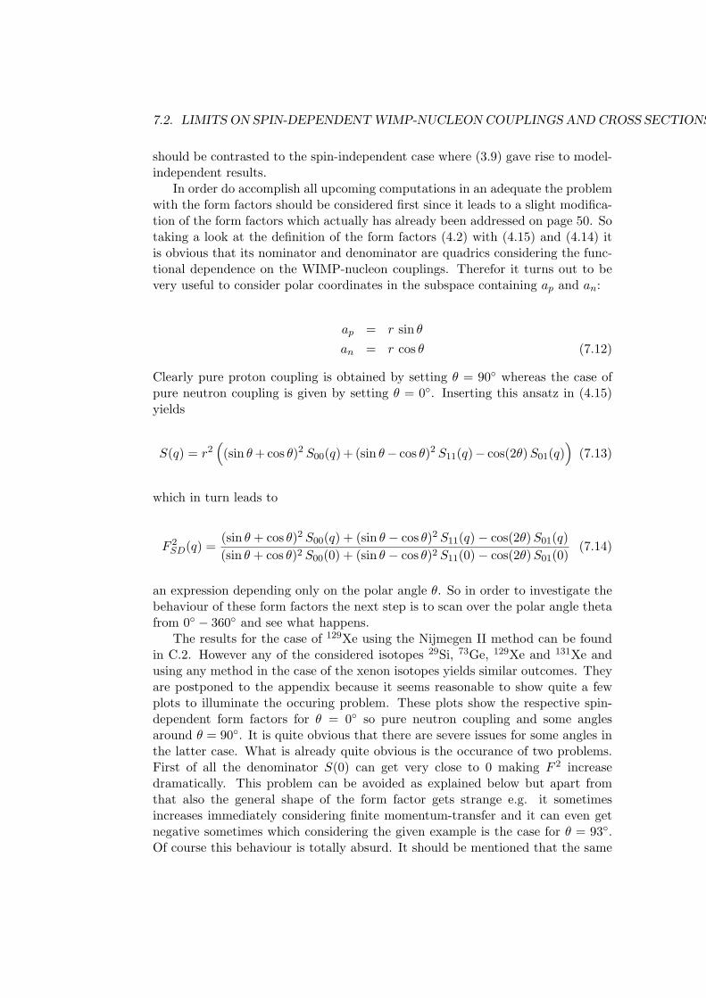
7.2. LIMITS ON SPIN-DEPENDENT WIMP-NUCLEON COUPLINGS AND CROSS SECTIONS103
should be contrasted to the spin-independent case where (3.9) gave rise to model-independent results.
In order do accomplish all upcoming computations in an adequate the problemwith the form factors should be considered first since it leads to a slight modifica-tion of the form factors which actually has already been addressed on page 50. Sotaking a look at the definition of the form factors (4.2) with (4.15) and (4.14) itis obvious that its nominator and denominator are quadrics considering the func-tional dependence on the WIMP-nucleon couplings. Therefor it turns out to bevery useful to consider polar coordinates in the subspace containing ap and an:
ap = r sin θan = r cos θ (7.12)
Clearly pure proton coupling is obtained by setting θ = 90 whereas the case ofpure neutron coupling is given by setting θ = 0. Inserting this ansatz in (4.15)yields
S(q) = r2(
(sin θ+ cos θ)2 S00(q) + (sin θ− cos θ)2 S11(q)− cos(2θ)S01(q))
(7.13)
which in turn leads to
F 2SD(q) =
(sin θ + cos θ)2 S00(q) + (sin θ − cos θ)2 S11(q)− cos(2θ)S01(q)(sin θ + cos θ)2 S00(0) + (sin θ − cos θ)2 S11(0)− cos(2θ)S01(0)
(7.14)
an expression depending only on the polar angle θ. So in order to investigate thebehaviour of these form factors the next step is to scan over the polar angle thetafrom 0 − 360 and see what happens.
The results for the case of 129Xe using the Nijmegen II method can be foundin C.2. However any of the considered isotopes 29Si, 73Ge, 129Xe and 131Xe andusing any method in the case of the xenon isotopes yields similar outcomes. Theyare postponed to the appendix because it seems reasonable to show quite a fewplots to illuminate the occuring problem. These plots show the respective spin-dependent form factors for θ = 0 so pure neutron coupling and some anglesaround θ = 90. It is quite obvious that there are severe issues for some angles inthe latter case. What is already quite obvious is the occurance of two problems.First of all the denominator S(0) can get very close to 0 making F 2 increasedramatically. This problem can be avoided as explained below but apart fromthat also the general shape of the form factor gets strange e.g. it sometimesincreases immediately considering finite momentum-transfer and it can even getnegative sometimes which considering the given example is the case for θ = 93.Of course this behaviour is totally absurd. It should be mentioned that the same
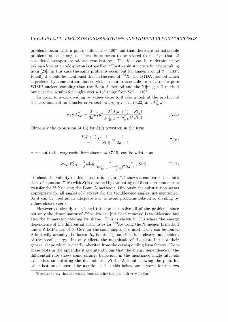
104CHAPTER 7. LIMITS ON CROSS SECTIONS AND WIMP-NUCLEON COUPLINGS
problems occur with a phase shift of θ = 180 and that there are no noticeableproblems at other angles. These issues seem to be related to the fact that allconsidered isotopes are odd-neutron isotopes. This idea can be underpinned bytaking a look at an odd-proton isotope like 127I with spin structure functions takingfrom [28]. In this case the same problems occur but for angles around θ = 180.Finally it should be mentioned that in the case of 131Xe the QTDA method whichis prefered by some authors indeed yields a more reasonable form factor for pureWIMP nucleon coupling than the Bonn A method and the Nijmegen II methodbut negative results for angles over a 15 range from 95 − 110.
In order to avoid dividing by values close to 0 take a look at the product ofthe zero-momentum transfer cross section σSD given in (3.22) and F 2
SD:
σSD F2SD =
23πµ2T g
41
Λ2J(J + 1)(m2
B(1) −m2q(1)
)2
S(q)S(0)
(7.15)
Obviously the expression (4.13) for S(0) rewritten in the form
J(J + 1)π
Λ2 1S(0)
=1
2J + 1(7.16)
turns out to be very useful here since now (7.15) can be written as
σSD F2SD =
23µ2T g
41
1(m2
B(1) −m2q(1)
)2
12J + 1
S(q) . (7.17)
To check the validity of this substitution figure 7.5 shows a comparison of bothsides of equation (7.16) with S(0) obtained by evaluating (4.15) at zero-momentumtransfer for 131Xe using the Bonn A method.2 Obviously the substitution seemsappropriate for all angles of θ except for the troublesome angles just mentioned.So it can be used as an adequate way to avoid problems related to dividing byvalues close to zero.
However as already mentioned this does not solve all of the problems sincenot only the denominator of F 2 which has just been removed is troublesome butalso the numerator yielding its shape. This is shown in C.3 where the energydependence of the differential event rates for 129Xe using the Nijmegen II methodand a WIMP mass of 50 GeV for the same angles of θ used in C.2 can be found.Admittedly actually the factor R0 is missing but since it is clearly independentof the recoil energy this only effects the magnitude of the plots but not theirgeneral shape which is clearly inherited from the corresponding form factors. Fromthese plots in the appendix it is quite obvious that the energy dependence of thedifferential rate shows some strange behaviour in the mentioned angle intervalseven after substituting the denominator S(0). Without showing the plots forother isotopes it should be mentioned that this behaviour is worst for the two
2Needless to say that the results from all other isotopes look very similar.
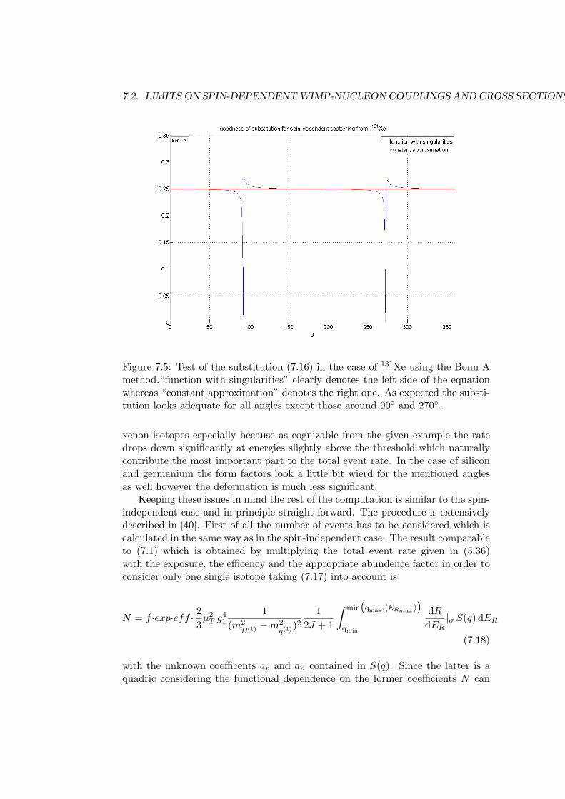
7.2. LIMITS ON SPIN-DEPENDENT WIMP-NUCLEON COUPLINGS AND CROSS SECTIONS105
Figure 7.5: Test of the substitution (7.16) in the case of 131Xe using the Bonn Amethod.“function with singularities” clearly denotes the left side of the equationwhereas “constant approximation” denotes the right one. As expected the substi-tution looks adequate for all angles except those around 90 and 270.
xenon isotopes especially because as cognizable from the given example the ratedrops down significantly at energies slightly above the threshold which naturallycontribute the most important part to the total event rate. In the case of siliconand germanium the form factors look a little bit wierd for the mentioned anglesas well however the deformation is much less significant.
Keeping these issues in mind the rest of the computation is similar to the spin-independent case and in principle straight forward. The procedure is extensivelydescribed in [40]. First of all the number of events has to be considered which iscalculated in the same way as in the spin-independent case. The result comparableto (7.1) which is obtained by multiplying the total event rate given in (5.36)with the exposure, the efficency and the appropriate abundence factor in order toconsider only one single isotope taking (7.17) into account is
N = f ·exp·eff · 23µ2T g
41
1(m2
B(1) −m2q(1)
)2
12J + 1
∫ min(
qmax,〈ERmax 〉)
qmin
dRdER
|σ S(q) dER
(7.18)
with the unknown coefficents ap and an contained in S(q). Since the latter is aquadric considering the functional dependence on the former coefficients N can
106CHAPTER 7. LIMITS ON CROSS SECTIONS AND WIMP-NUCLEON COUPLINGS
be written in the form
N = Aa2p + 2B apan + C a2
n (7.19)
with the values A, B and C which are constant for a given WIMP mass whichwill be assumed at the moment:
A = f · exp · eff · 23µ2T g
41
1(m2
B(1) −m2q(1)
)2
12J + 1
·∫ min
(qmax,〈ERmax 〉
)qmin
dRdER
|σ(S00(q) + S11(q) + S01(q)
)dER
B = f · exp · eff · 23µ2T g
41
1(m2
B(1) −m2q(1)
)2
12J + 1
·∫ min
(qmax,〈ERmax 〉
)qmin
dRdER
|σ(S00(q) + S11(q)− S01(q)
)dER
C = f · exp · eff · 23µ2T g
41
1(m2
B(1) −m2q(1)
)2
12J + 1
·∫ min
(qmax,〈ERmax 〉
)qmin
dRdER
|σ(S00(q)− S11(q)
)dER . (7.20)
In order to get a certain idea about the different types of solutions which arepossible it is appropriate to remember that the quadric (7.19) describes a conic inthe ap vs. an-plane. However since there are no linear terms in ap or an this is notthe general form of a second degree polynomial and only three different types ofsolutions are possible which are furthermore all centered at the origin. These areellipses, hyperbolas and two parallel straight lines3 which can be written in thefollowing forms respectively:
x2
a2+y2
b2= 1 ,
x2
a2− y2
b2= 1 , x2 = a2 (7.21)
where all cross terms leading to a rotation in the x vs. y-plane have been sur-pressed. However from taking a look at (7.19) rotations definitely occur. Theactual type of conic is clearly determined by the relative magnitudes of the coeffi-cients A, B and C which crucially depend on the WIMP mass and the structurefunctions. Mathematically the shape can be determined by computing
D := det(B CA B
)= B2 −AC . (7.22)
D < 0 corresponds to an ellipse whereas D = 0 correponds to two parallel straight3Two parallel straight lines are in fact called a degenerate conic.
7.2. LIMITS ON SPIN-DEPENDENT WIMP-NUCLEON COUPLINGS AND CROSS SECTIONS107
lines and D > 0 to a hyperbola. Considering all isotopes for the masses discussedbelow negative values were obtained so that the only occuring shape is an ellipse.Hence the eigenvectors of the matrix given in (7.22) yield the direction of themajor axis and the inverse eigenvalues their lengths.
However it turns out to be much more appropriate to use the polar coordinatesintroduced in (7.12) which gives rise to
N = r2(A sin2 θ + 2B sin θ cos θ + C cos2 θ
). (7.23)
This in turn can be rewritten as
r2 =N(
A sin2 θ + 2B sin θ cos θ + C cos2 θ) (7.24)
which should be compared to (7.2). The most important difference between thesetwo expressions apart from the troublesome form factors determining A, B and Cis that even for a fixed WIMP mass the right side of (7.24) is clearly not constantdue to the dependence on θ.
So computing limits on the WIMP-nucleon couplings is accomplished as fol-lows: For any WIMP mass of interest perform a scan over the angle θ from 0−360
which leads to a constant denominator in (7.24). Hence a limit on r2 can becomputed in exactly the same way as in the spin-independent case using the Feld-man & Cousins method as well as the Maximum Gap method. Thus since thedeterminante D given in (7.22) yielded negative values each time the results areexpected to be ellipses in the ap vs. an plane for each considered WIMP mass. Sothe ap-an parameter space is restricted to the inner region of these ellipses. If aWIMP signal would be observed this analysis would yield two concentric ellipseswith the obtained band representing the permitted region and its thickness beingdefined by the uncertainty in the observed signal.
Of course for a proper analysis it is necessary to scan over a reasonable intervalof WIMP masses as well starting with the minimal WIMP masses yielding recoilenergies above the threshold given in table 5.1. Since ellipses are obtained for eachfixed WIMP mass the result is clearly a closed surface shaped as a tube consideringthe full 3-dimensional parameter space.4 However a more useful form is to onlyconsider the ellipses for a few fixed WIMP masses since it is difficult to extractproper results from 3-dimensional plots. Several plots showing the obtained resultscan be found below after the discussion of another though less exact method tocompute limits in the ap vs. an plane.
But before proceeding with the description of this method a short insertion.Apart from the computation of limits on WIMP-nucleon couplings for a givenWIMP mass it is quite interesting to calculate limits on the WIMP-neutron cross
4A plot like this can be found in C.6 but for neutralino-nucleon scattering. The reason toconsider this model as well is discussed later on.
108CHAPTER 7. LIMITS ON CROSS SECTIONS AND WIMP-NUCLEON COUPLINGS
sections considering coupling solely to neutrons which means setting ap = 0 andthe other way around setting an = 0 to compute cross section limits for pureWIMP-proton coupling. However this can be achieved rather easily by remem-bering that the former case is equivalent to setting θ = 0 yielding an = r andthe latter to setting θ = 90 yielding ap = r. Hence the computed limits on r2
for θ = 0 and θ = 90 directly yield the important limits on pure WIMP-nucleoncouplings which can be converted to corresponding cross section limits using thenormalization given in (3.27). It is important to note that the obtained limits onthe pure WIMP-nucleon cross sections are model independent which is evidentfrom (3.27).
Since obtained results considering pure coupling to protons differ very muchfrom the corresponding results considering pure coupling to neutrons both caseshave to be shown separately. This is accomplished in the figures 7.6 and 7.7 forsilicon, in 7.8 and 7.9 for germanium and 7.10 and 7.11 for xenon using the Bonn Amethod with the results from both xenon isotopes combined using (7.5). Asexpected the limits considering pure coupling to neutrons are much more stringentthan the limits related to pure coupling to protons with a difference of about afactor of 100− 1000. General annotations about the shape of the curves and thecomparison of the Feldman & Cousins method and Maximum Gap method can befound in the corresponding discussion of limits on spin-independent cross sections.
Of course in order to accomplish a comparison between these computed limitsand theoretical predictions it is useful to plot all results in two figures one for thecoupling to neutrons and another one for the coupling to protons. The theoreticalpredictions are taken from the figures 3.7 and 3.6 respecively. Moreover similarto the spin-independent case the results considering the Maximum Gap methodare used for the comparisons. They can be found in the figures 7.12 and 7.13respectively. Obviously the XENON10 experiment yields the most stringent limitson these cross sections in both cases. However the results from germanium targetsare quite good as well despite of the low abundance of 73Ge. However they areweaker approximately by a factor of 10. An important observation is the factthat even considering the results from XENON10 and pure coupling to neutronsthe limits are about a factor of 100 to high to probe the interesting parameterspace for WIMP masses of 500 GeV. Before proceeding an important annotationhas to be made considering the spin-dependent limits assuming pure couplingto protons or rather θ = 90. Taking a look at the corresponding differentialevent rate for 129Xe using the Nijmegen II potential given in C.3 indicates thatthis curve is to high due to the mentioned form factor problems. Of course thisleads to a lower upper limit on the corresponding cross section. An appropriateform factor would certainly yield less stringent results. Since the cross sectionlimits corresponding to this kind of interaction are generally less interesting sinceodd-proton isotopes naturally yield better results this does not seem to be a realproblem. However they are a crucial input to the other method used to computelimits in the ap vs. an plane just mentioned which is described below. This willturn out to be an important problem of this procedure.
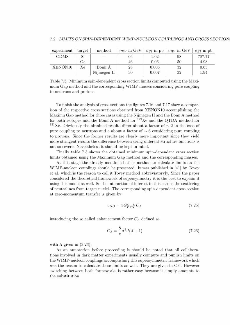
7.2. LIMITS ON SPIN-DEPENDENT WIMP-NUCLEON COUPLINGS AND CROSS SECTIONS109
experiment target method mW in GeV σSI in pb mW in GeV σSI in pbCDMS Si — 66 1.02 98 787.77
Ge — 46 0.06 50 4.98XENON10 Xe Bonn A 28 0.005 32 0.63
Nijmegen II 30 0.007 32 1.94
Table 7.3: Minimum spin-dependent cross section limits computed using the Maxi-mum Gap method and the corresponding WIMP masses considering pure couplingto neutrons and protons.
To finish the analysis of cross sections the figures 7.16 and 7.17 show a compar-ison of the respective cross sections obtained from XENON10 accomplishing theMaximu Gap method for three cases using the Nijmegen II and the Bonn A methodfor both isotopes and the Bonn A method for 129Xe and the QTDA method for131Xe. Obviously the obtained results differ about a factor of ∼ 2 in the case ofpure coupling to neutrons and a about a factor of ∼ 6 considering pure couplingto protons. Since the former results are clearly more important since they yieldmore stringent results the difference between using different structure functions isnot so severe. Nevertheless it should be kept in mind.
Finally table 7.3 shows the obtained minimum spin-dependent cross sectionlimits obtained using the Maximum Gap method and the corresponding masses.
At this stage the already mentioned other method to calculate limits on theWIMP-nucleon couplings should be presented. It was published in [41] by Toveyet al. which is the reason to call it Tovey method abbreviatoryly. Since the paperconsidered the theoretical framework of supersymmetry it is the best to explain itusing this model as well. So the interaction of interest in this case is the scatteringof neutralinos from target nuclei. The corresponding spin-dependent cross sectionat zero-momentum transfer is given by
σSD = 4G2F µ
2T CA (7.25)
introducing the so called enhancement factor CA defined as
CA =8π
Λ2J(J + 1) (7.26)
with Λ given in (3.23).As an annotation before proceeding it should be noted that all collabora-
tions involved in dark matter experiments usually compute and puplish limits onthe WIMP-nucleon couplings accomplishing this supersymmetric framework whichwas the reason to calculate these limits as well. They are given in C.6. Howeverswitching between both frameworks is rather easy because it simply amounts tothe substitution
110CHAPTER 7. LIMITS ON CROSS SECTIONS AND WIMP-NUCLEON COUPLINGS
Susy ←→ UED
G2F ←→ 1
48g4
1
(m2B(1) −m2
q(1))2
(7.27)
which is evident from comparing (7.25) to (3.22).In order to continue the discussion of the Tovey method the enhancement
factor can be written as
CA =8π
(|ap〈Sp〉| ± |an〈Sn〉|
)2 J + 1J
=(√
CpA ±√CnA
)2(7.28)
where the relative sign inside the square is given by the sign of ap〈Sp〉an〈Sn〉 and the
proton and neutron contributions are defined as
CpA =8π
(ap〈Sp〉
)2J + 1J
CnA =8π
(an〈Sn〉
)2J + 1J
. (7.29)
Using these definitions the contributions of both nucleons to the cross section(7.25) can be separated similarly using
σpA = 4G2F µ
2T C
pA
σnA = 4G2F µ
2T C
nA (7.30)
yielding
σSD =(√
σpA ±√σnA
)2. (7.31)
Note that the quantities σpA and σnA are nothing but convenient auxiliary quantitieswhich however do not represent measurable cross sections. Hence (7.28) and (7.25)can be evaluated for single nucleons leading to
Cp =6πa2p
Cn =6πa2n (7.32)
and thus to
7.2. LIMITS ON SPIN-DEPENDENT WIMP-NUCLEON COUPLINGS AND CROSS SECTIONS111
σp = σpAµ2p
µ2T
CpCpA
σn = σnAµ2n
µ2T
CnCpA
(7.33)
Now comes an approximation which obviously is not necessary accomplishing theθ scan explained before. Since as already mentioned the quantities introduced in(7.30) are not measurable quantities the authors made the assumptions
σpA ≈ σSD and σnA ≈ σSD (7.34)
independently which together with the renamings σp → σAp and σn → σAn in thiscase leads to
σAp = σAµ2p
µ2T
CpCpA
σAn = σAµ2n
µ2T
CnCpA
(7.35)
So the quantities σAp and σAn denote the WIMP-nucleon cross sections assumingthat it is dominated by the proton and neutron contribution respectively. Com-paring (7.33) and (7.35) directly yields the two relations
σpσAp
=σpAσSD
andσnσAn
=σnAσSD
(7.36)
Expressing σp and σn in terms of the WIMP-nucleon couplings and neglecting thedifference between the proton and neutron mass inserting (7.36) into (7.31) leadsto the final result given by ap√
σAp
± an√σAn
2
=π
24G2Fµ
2n
(7.37)
which can be translated to the UED framework using (7.27): ap√σAp
± an√σAn
2
=2π(m2
B(1) −m2q(1)
)2
g41µ
2n
(7.38)
Note that the sign in the brackets of both equations is given by the sign of 〈Sp〉〈Sn〉 .
112CHAPTER 7. LIMITS ON CROSS SECTIONS AND WIMP-NUCLEON COUPLINGS
According to their definition limits on σAp and σAn are set by the already discussedcross section limits considering pure coupling to protons and neutrons respectively.Since (7.27) and (7.38) actually define two parallel lines it is clear that the exteriorof these two lines is excluded. Taking a closer look at the definitions of these linesit is clear that the method only puts straight lines through the points of purecoupling in the ap vs. an plane. Moreover their slope m is given by
m = − sign(〈Sp〉〈Sn〉
)√σApσAn≈ −〈Sn〉〈Sp〉
(7.39)
The authors argue that the last “≈” holds exactly. In fact it can be derivedby using the expression (3.28) assuming that the obtained cross section limit isequal for pure proton and pure neutron coupling. However it is not which is cleardue to the accomplishment of different form factors in each case. Neverthelessusing a form factor which is constant with respect to the couplings leads to theirresult. This is accomplished for example by the Zeplin-II collaboration as statedin [42]. According to this paper they used a form factor arising from higgsinointeractions which is particularly small so that the resulting limits are expectedto be conservative.
Finally it should be mentioned that it seems that all collaborations searchingfor dark matter using direct detection use the just explained Tovey method.
After this extensive discussion it is time to take a look at the final results of thecomputation of setting limits on the WIMP-nucleon couplings. The figures 7.18,7.19, 7.20 and 7.21 show these results for a fixed WIMP mass of mB(1) = 50 GeVand a degeneracy parameter of ∆ = 0.15 for all odd-nucleon targets. Moreoverthe theoretical predictions given in (3.26) are included in these plots as well.
The θ scan and the Tovey method combined with the Feldman & Cousinsmethod as well as the Maximum Gap method are used. Again the results ob-tained by the Maximum Gap method are more stringent than those using theFeldman & Cousins method. Moreover it is clear that the CDMS limits are alittle bit to severe due to the accomplishment of an efficiency of 0.4. Especiallyfrom the silicon results it is obvious that the limits from the Tovey method andthe θ scan are equal in the cases of pure nucleon coupling as expected. Moreoverit is obvious that 29Si is the only isotope where the lines determined by the Toveymethod have a positive slope. This can be explained by taking a look at the spinexpectation values given in table 4.1.
The general orientation of the obtained ellipses or rather parallel lines is alsoclear. Since all isotopes have an unpaired neutron limits on ap are much weakerthan on an. Hence the allowed regions are almost aligned with the ap-axis. Thisalignment is not exact since each isotope has only a little but nevertheless nota vanishing sensitivity to pure WIMP-proton coupling. Note that allowing non-vanishing values of both an and ap the limits on each can be considerably weak-ened. Consider for example the shown limits computed using 73Ge. Assuming
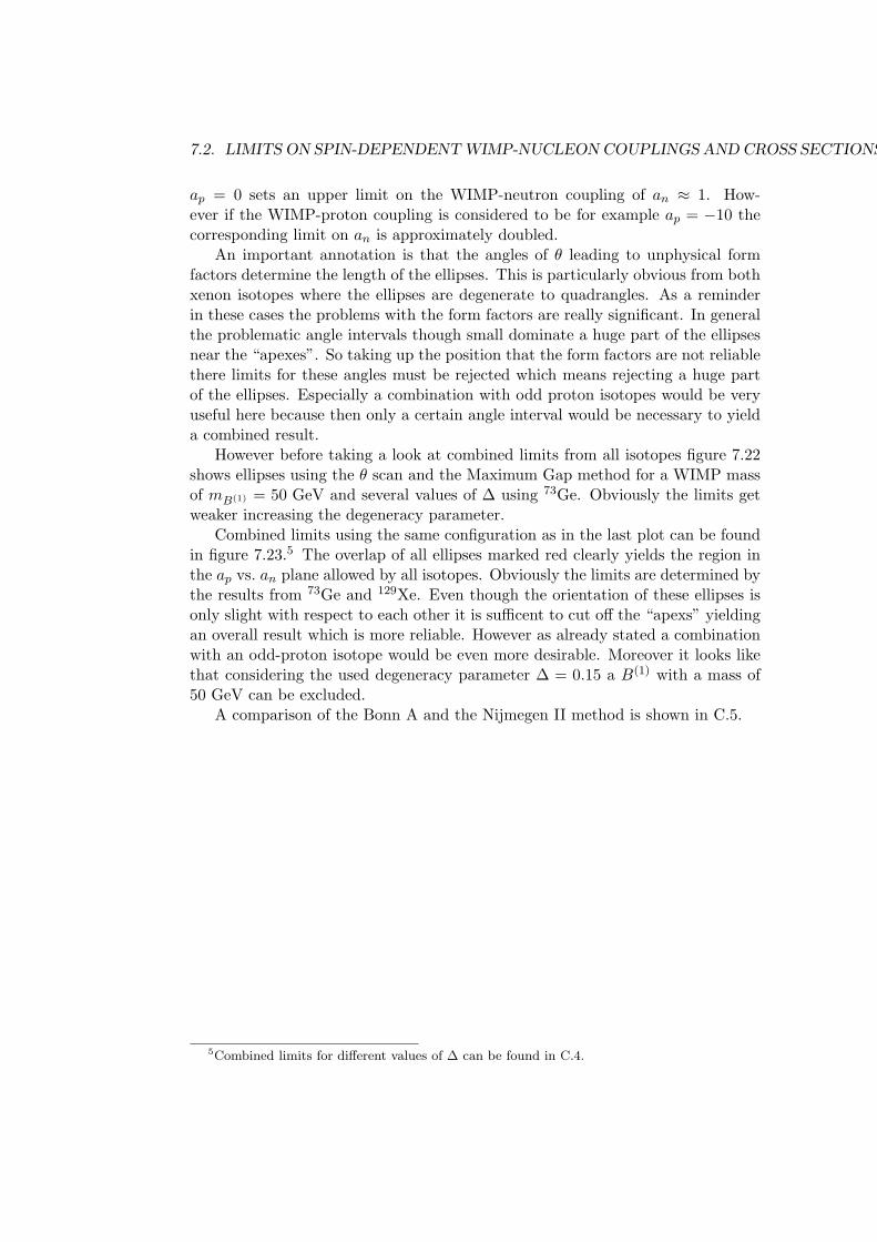
7.2. LIMITS ON SPIN-DEPENDENT WIMP-NUCLEON COUPLINGS AND CROSS SECTIONS113
ap = 0 sets an upper limit on the WIMP-neutron coupling of an ≈ 1. How-ever if the WIMP-proton coupling is considered to be for example ap = −10 thecorresponding limit on an is approximately doubled.
An important annotation is that the angles of θ leading to unphysical formfactors determine the length of the ellipses. This is particularly obvious from bothxenon isotopes where the ellipses are degenerate to quadrangles. As a reminderin these cases the problems with the form factors are really significant. In generalthe problematic angle intervals though small dominate a huge part of the ellipsesnear the “apexes”. So taking up the position that the form factors are not reliablethere limits for these angles must be rejected which means rejecting a huge partof the ellipses. Especially a combination with odd proton isotopes would be veryuseful here because then only a certain angle interval would be necessary to yielda combined result.
However before taking a look at combined limits from all isotopes figure 7.22shows ellipses using the θ scan and the Maximum Gap method for a WIMP massof mB(1) = 50 GeV and several values of ∆ using 73Ge. Obviously the limits getweaker increasing the degeneracy parameter.
Combined limits using the same configuration as in the last plot can be foundin figure 7.23.5 The overlap of all ellipses marked red clearly yields the region inthe ap vs. an plane allowed by all isotopes. Obviously the limits are determined bythe results from 73Ge and 129Xe. Even though the orientation of these ellipses isonly slight with respect to each other it is sufficent to cut off the “apexs” yieldingan overall result which is more reliable. However as already stated a combinationwith an odd-proton isotope would be even more desirable. Moreover it looks likethat considering the used degeneracy parameter ∆ = 0.15 a B(1) with a mass of50 GeV can be excluded.
A comparison of the Bonn A and the Nijmegen II method is shown in C.5.
5Combined limits for different values of ∆ can be found in C.4.
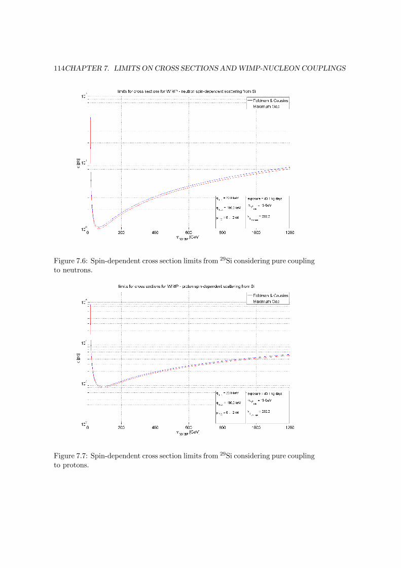
114CHAPTER 7. LIMITS ON CROSS SECTIONS AND WIMP-NUCLEON COUPLINGS
Figure 7.6: Spin-dependent cross section limits from 29Si considering pure couplingto neutrons.
Figure 7.7: Spin-dependent cross section limits from 29Si considering pure couplingto protons.
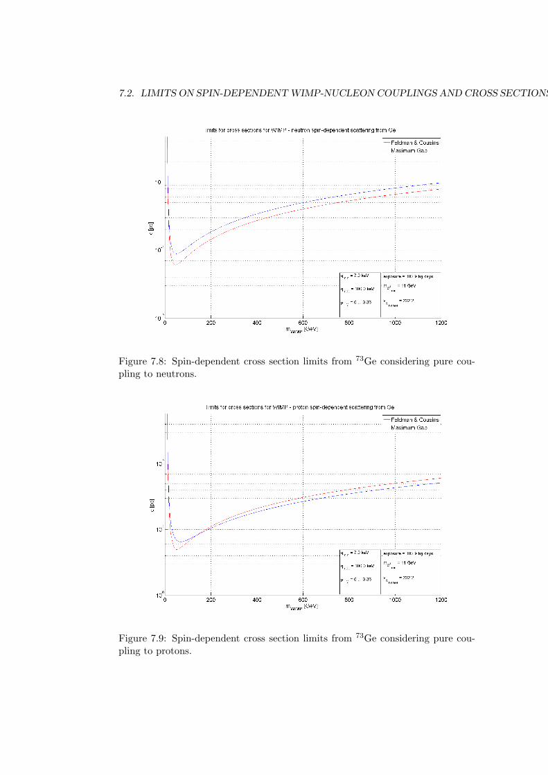
7.2. LIMITS ON SPIN-DEPENDENT WIMP-NUCLEON COUPLINGS AND CROSS SECTIONS115
Figure 7.8: Spin-dependent cross section limits from 73Ge considering pure cou-pling to neutrons.
Figure 7.9: Spin-dependent cross section limits from 73Ge considering pure cou-pling to protons.
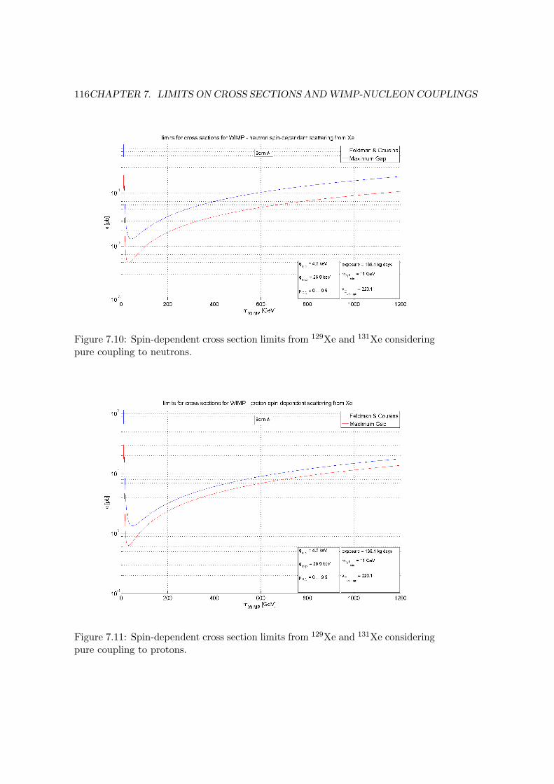
116CHAPTER 7. LIMITS ON CROSS SECTIONS AND WIMP-NUCLEON COUPLINGS
Figure 7.10: Spin-dependent cross section limits from 129Xe and 131Xe consideringpure coupling to neutrons.
Figure 7.11: Spin-dependent cross section limits from 129Xe and 131Xe consideringpure coupling to protons.
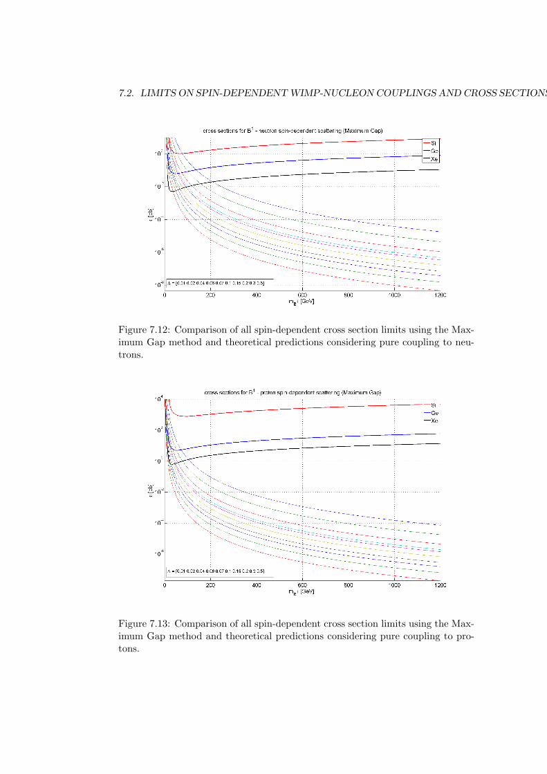
7.2. LIMITS ON SPIN-DEPENDENT WIMP-NUCLEON COUPLINGS AND CROSS SECTIONS117
Figure 7.12: Comparison of all spin-dependent cross section limits using the Max-imum Gap method and theoretical predictions considering pure coupling to neu-trons.
Figure 7.13: Comparison of all spin-dependent cross section limits using the Max-imum Gap method and theoretical predictions considering pure coupling to pro-tons.
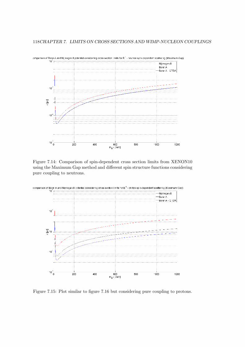
118CHAPTER 7. LIMITS ON CROSS SECTIONS AND WIMP-NUCLEON COUPLINGS
Figure 7.14: Comparison of spin-dependent cross section limits from XENON10using the Maximum Gap method and different spin structure functions consideringpure coupling to neutrons.
Figure 7.15: Plot similar to figure 7.16 but considering pure coupling to protons.
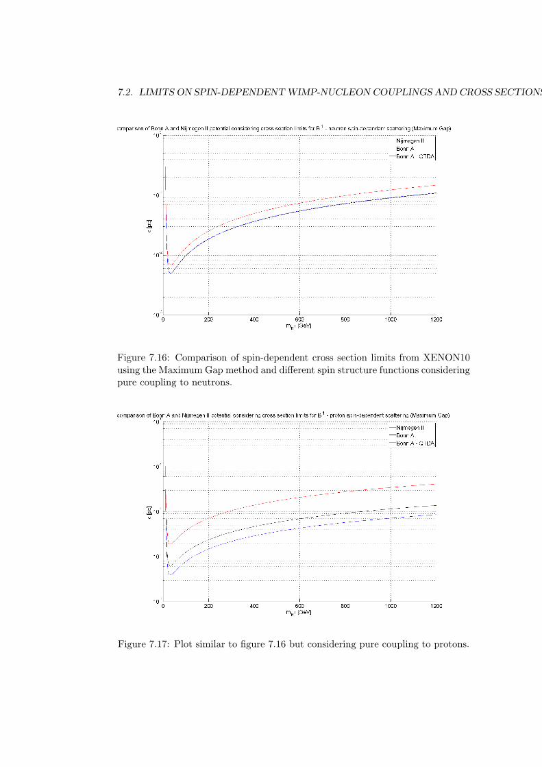
7.2. LIMITS ON SPIN-DEPENDENT WIMP-NUCLEON COUPLINGS AND CROSS SECTIONS119
Figure 7.16: Comparison of spin-dependent cross section limits from XENON10using the Maximum Gap method and different spin structure functions consideringpure coupling to neutrons.
Figure 7.17: Plot similar to figure 7.16 but considering pure coupling to protons.
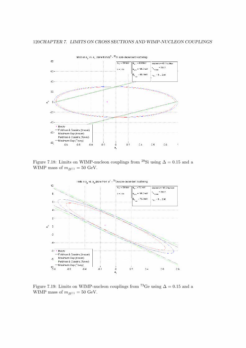
120CHAPTER 7. LIMITS ON CROSS SECTIONS AND WIMP-NUCLEON COUPLINGS
Figure 7.18: Limits on WIMP-nucleon couplings from 29Si using ∆ = 0.15 and aWIMP mass of mB(1) = 50 GeV.
Figure 7.19: Limits on WIMP-nucleon couplings from 73Ge using ∆ = 0.15 and aWIMP mass of mB(1) = 50 GeV.
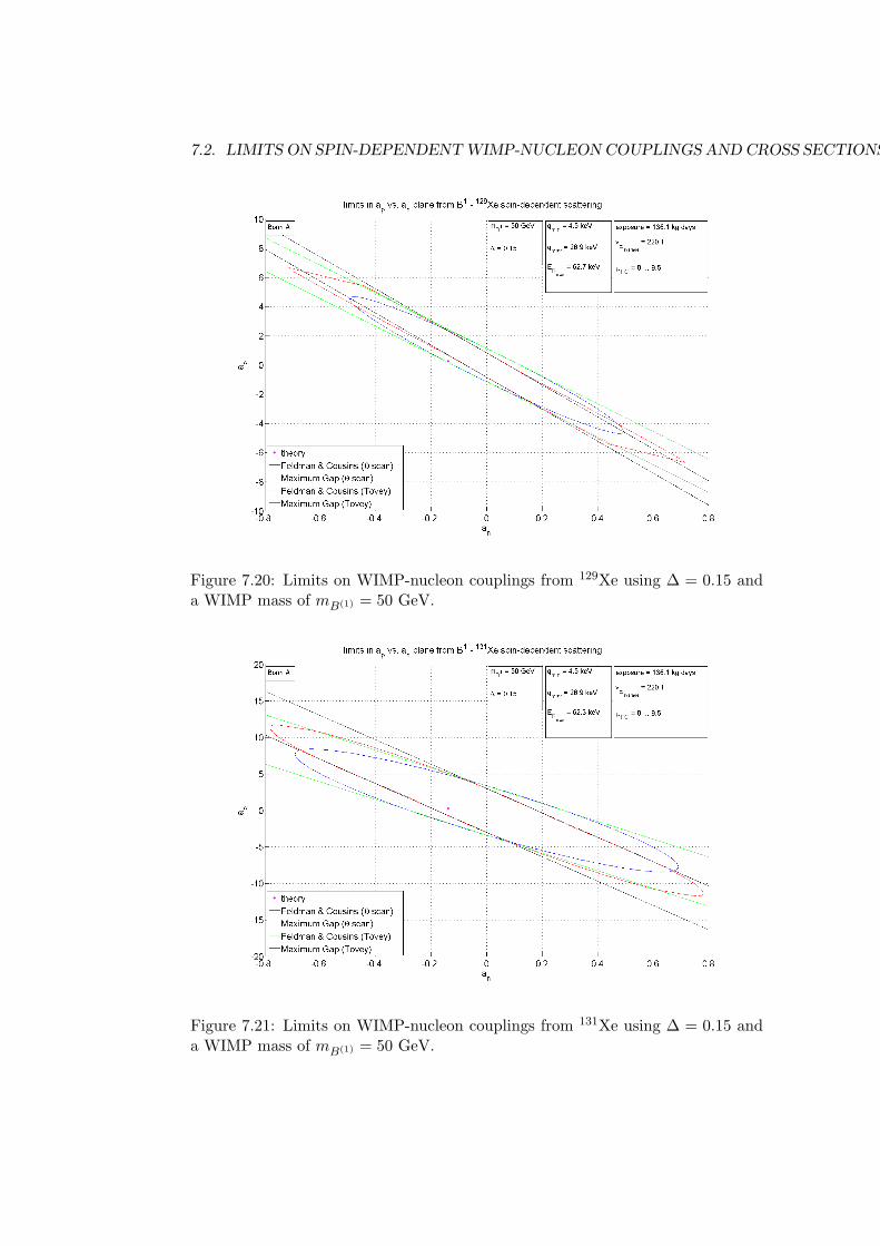
7.2. LIMITS ON SPIN-DEPENDENT WIMP-NUCLEON COUPLINGS AND CROSS SECTIONS121
Figure 7.20: Limits on WIMP-nucleon couplings from 129Xe using ∆ = 0.15 anda WIMP mass of mB(1) = 50 GeV.
Figure 7.21: Limits on WIMP-nucleon couplings from 131Xe using ∆ = 0.15 anda WIMP mass of mB(1) = 50 GeV.
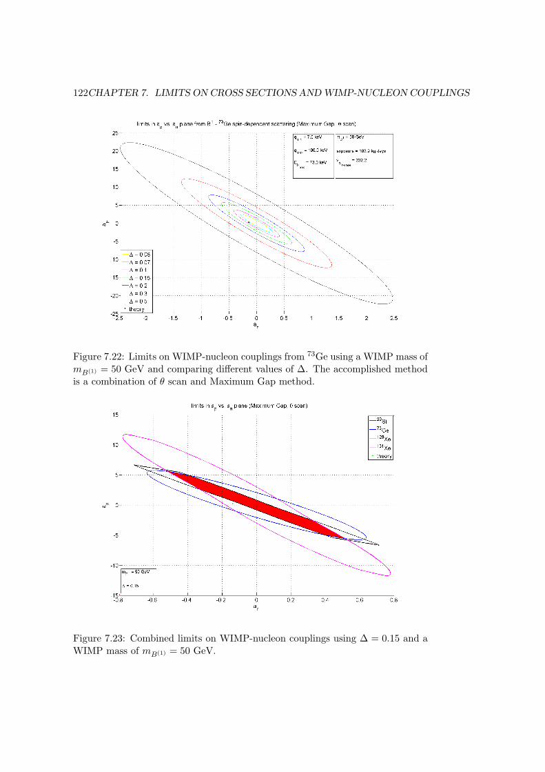
122CHAPTER 7. LIMITS ON CROSS SECTIONS AND WIMP-NUCLEON COUPLINGS
Figure 7.22: Limits on WIMP-nucleon couplings from 73Ge using a WIMP mass ofmB(1) = 50 GeV and comparing different values of ∆. The accomplished methodis a combination of θ scan and Maximum Gap method.
Figure 7.23: Combined limits on WIMP-nucleon couplings using ∆ = 0.15 and aWIMP mass of mB(1) = 50 GeV.
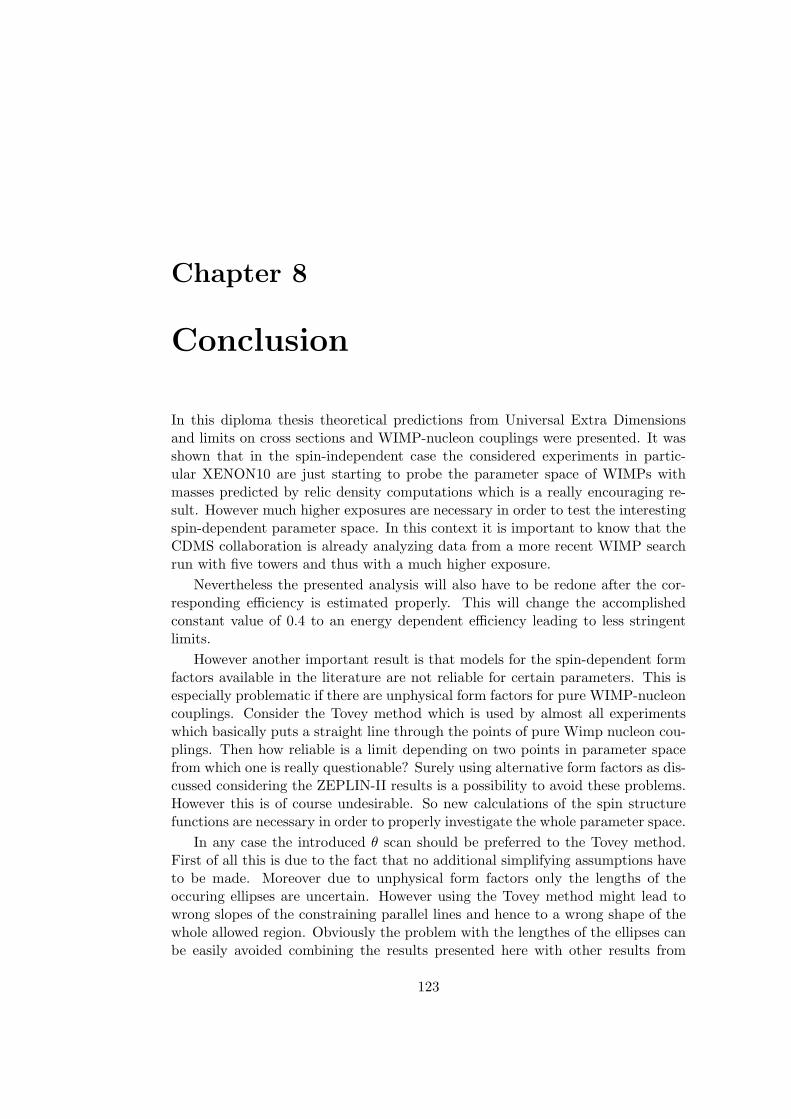
Chapter 8
Conclusion
In this diploma thesis theoretical predictions from Universal Extra Dimensionsand limits on cross sections and WIMP-nucleon couplings were presented. It wasshown that in the spin-independent case the considered experiments in partic-ular XENON10 are just starting to probe the parameter space of WIMPs withmasses predicted by relic density computations which is a really encouraging re-sult. However much higher exposures are necessary in order to test the interestingspin-dependent parameter space. In this context it is important to know that theCDMS collaboration is already analyzing data from a more recent WIMP searchrun with five towers and thus with a much higher exposure.
Nevertheless the presented analysis will also have to be redone after the cor-responding efficiency is estimated properly. This will change the accomplishedconstant value of 0.4 to an energy dependent efficiency leading to less stringentlimits.
However another important result is that models for the spin-dependent formfactors available in the literature are not reliable for certain parameters. This isespecially problematic if there are unphysical form factors for pure WIMP-nucleoncouplings. Consider the Tovey method which is used by almost all experimentswhich basically puts a straight line through the points of pure Wimp nucleon cou-plings. Then how reliable is a limit depending on two points in parameter spacefrom which one is really questionable? Surely using alternative form factors as dis-cussed considering the ZEPLIN-II results is a possibility to avoid these problems.However this is of course undesirable. So new calculations of the spin structurefunctions are necessary in order to properly investigate the whole parameter space.
In any case the introduced θ scan should be preferred to the Tovey method.First of all this is due to the fact that no additional simplifying assumptions haveto be made. Moreover due to unphysical form factors only the lengths of theoccuring ellipses are uncertain. However using the Tovey method might lead towrong slopes of the constraining parallel lines and hence to a wrong shape of thewhole allowed region. Obviously the problem with the lengthes of the ellipses canbe easily avoided combining the results presented here with other results from
123
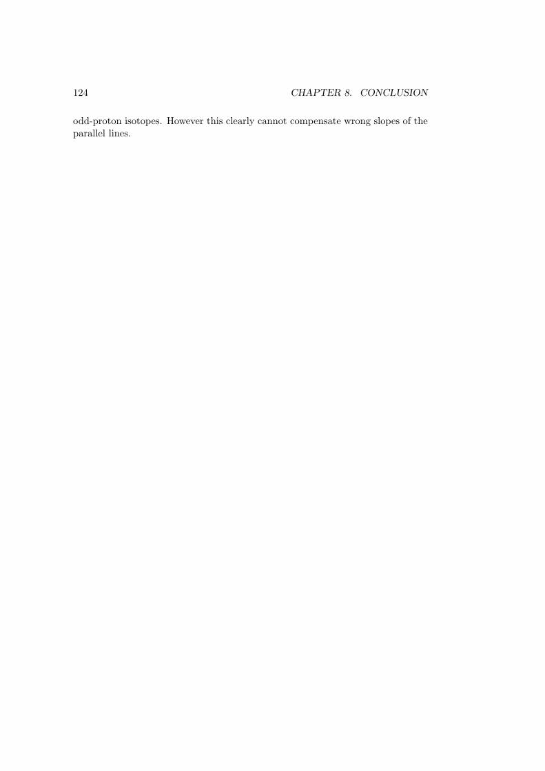
124 CHAPTER 8. CONCLUSION
odd-proton isotopes. However this clearly cannot compensate wrong slopes of theparallel lines.
Appendix A
Spin-independent cross sections
A.1 Spin-independent cross sections for fixed mH
In this part of the appendix some plots showing spin-independent B(1)-neutroncross sections for fixed values of the Higgs mass can be found. These figures aresimilar to figure 3.3 so an appropriate description of these plots can be foundthere. Obviously the dependence of the Higgs mass is rather weak.
125
126 APPENDIX A. SPIN-INDEPENDENT CROSS SECTIONS
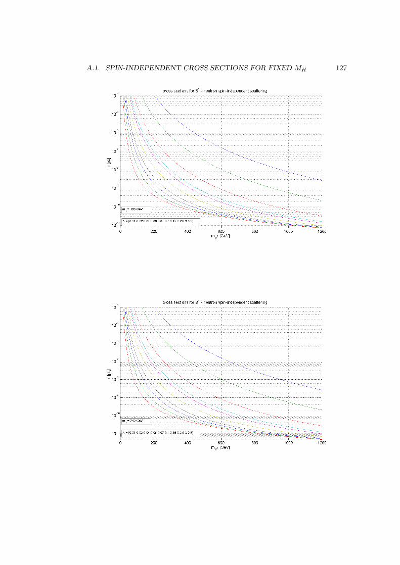
A.1. SPIN-INDEPENDENT CROSS SECTIONS FOR FIXED MH 127
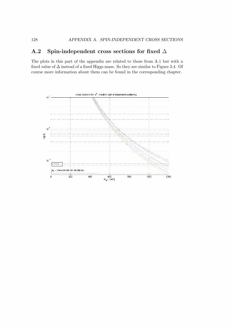
128 APPENDIX A. SPIN-INDEPENDENT CROSS SECTIONS
A.2 Spin-independent cross sections for fixed ∆
The plots in this part of the appendix are related to those from A.1 but with afixed value of ∆ instead of a fixed Higgs mass. So they are similar to Figure 3.4. Ofcourse more information about them can be found in the corresponding chapter.
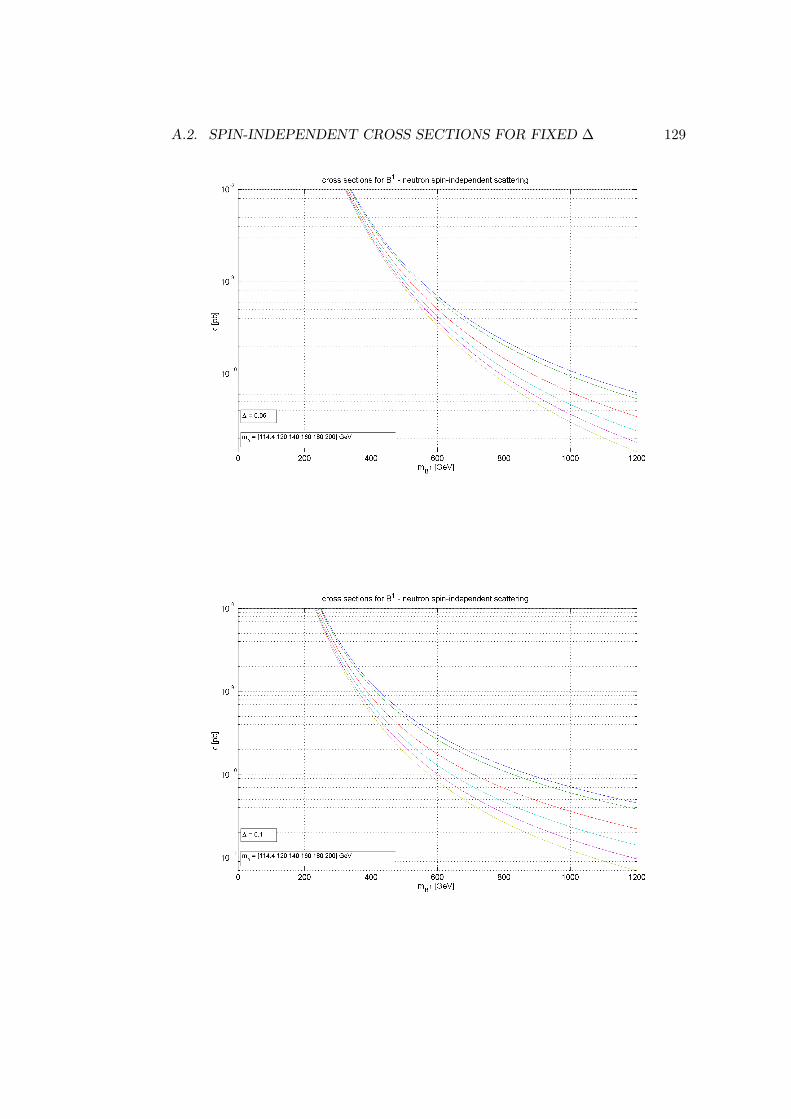
A.2. SPIN-INDEPENDENT CROSS SECTIONS FOR FIXED ∆ 129
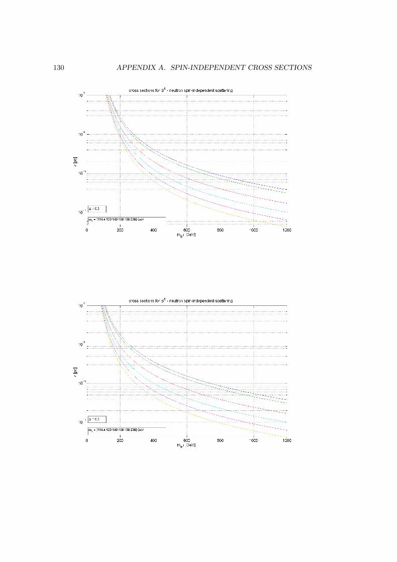
130 APPENDIX A. SPIN-INDEPENDENT CROSS SECTIONS
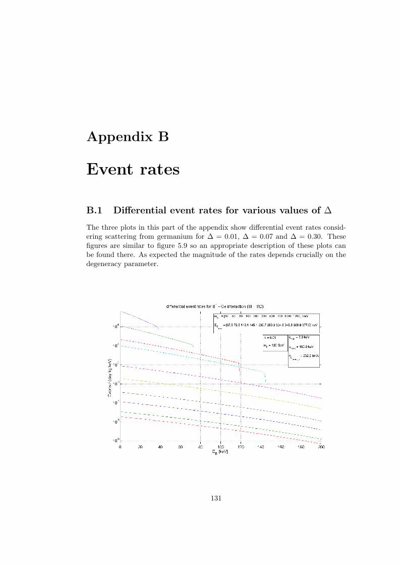
Appendix B
Event rates
B.1 Differential event rates for various values of ∆
The three plots in this part of the appendix show differential event rates consid-ering scattering from germanium for ∆ = 0.01, ∆ = 0.07 and ∆ = 0.30. Thesefigures are similar to figure 5.9 so an appropriate description of these plots canbe found there. As expected the magnitude of the rates depends crucially on thedegeneracy parameter.
131
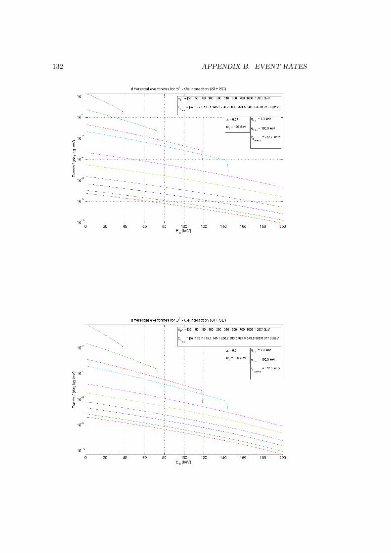
132 APPENDIX B. EVENT RATES
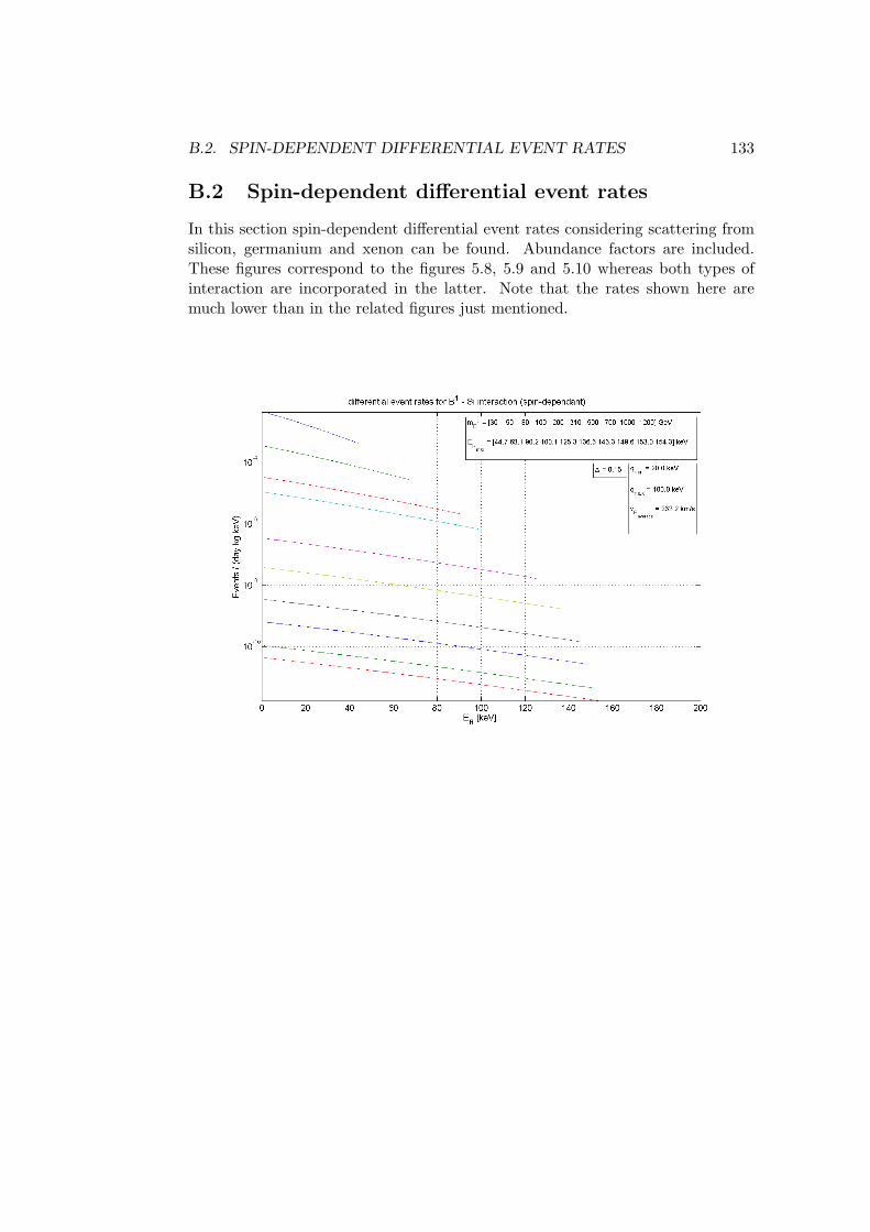
B.2. SPIN-DEPENDENT DIFFERENTIAL EVENT RATES 133
B.2 Spin-dependent differential event rates
In this section spin-dependent differential event rates considering scattering fromsilicon, germanium and xenon can be found. Abundance factors are included.These figures correspond to the figures 5.8, 5.9 and 5.10 whereas both types ofinteraction are incorporated in the latter. Note that the rates shown here aremuch lower than in the related figures just mentioned.
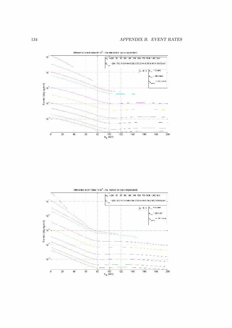
134 APPENDIX B. EVENT RATES
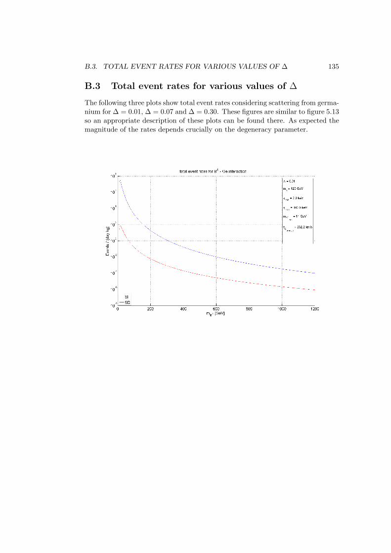
B.3. TOTAL EVENT RATES FOR VARIOUS VALUES OF ∆ 135
B.3 Total event rates for various values of ∆
The following three plots show total event rates considering scattering from germa-nium for ∆ = 0.01, ∆ = 0.07 and ∆ = 0.30. These figures are similar to figure 5.13so an appropriate description of these plots can be found there. As expected themagnitude of the rates depends crucially on the degeneracy parameter.
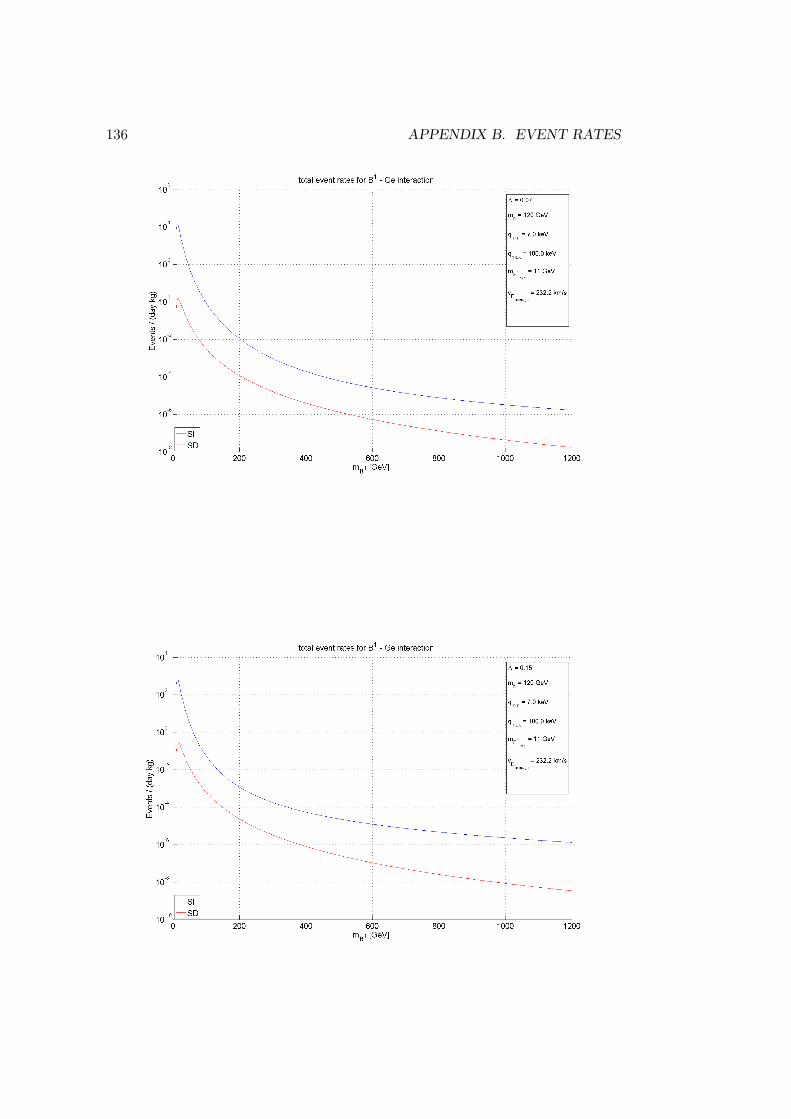
136 APPENDIX B. EVENT RATES
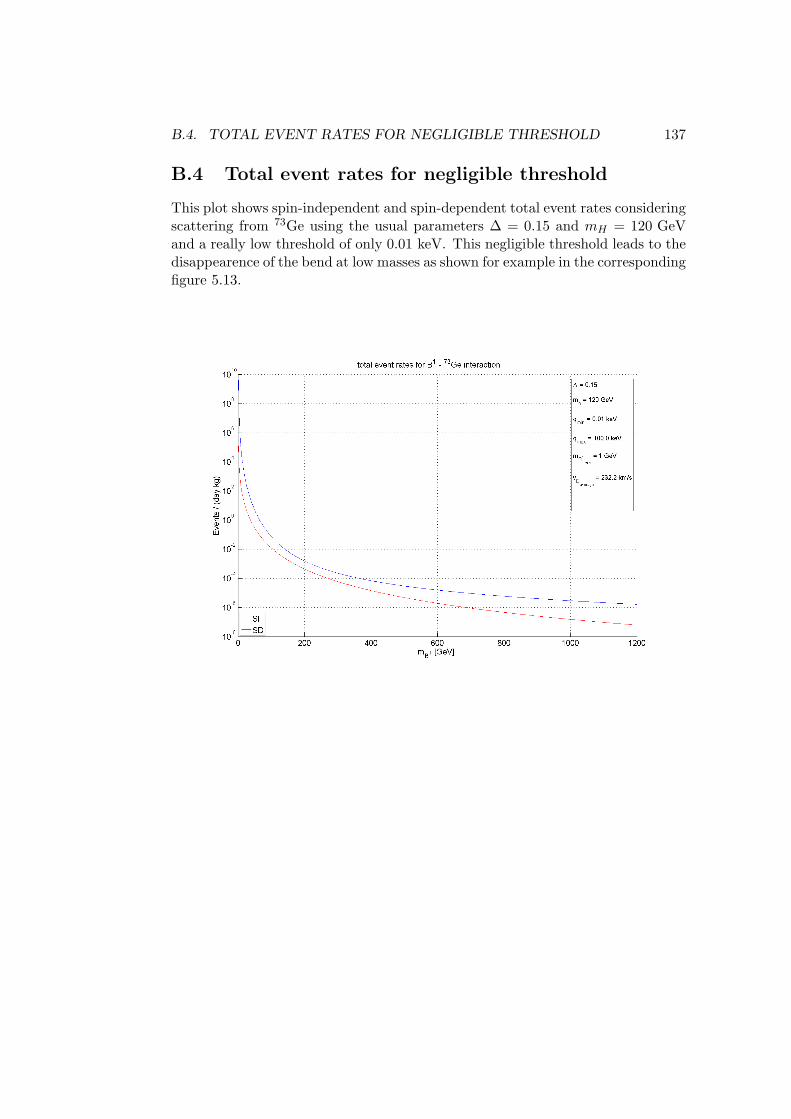
B.4. TOTAL EVENT RATES FOR NEGLIGIBLE THRESHOLD 137
B.4 Total event rates for negligible threshold
This plot shows spin-independent and spin-dependent total event rates consideringscattering from 73Ge using the usual parameters ∆ = 0.15 and mH = 120 GeVand a really low threshold of only 0.01 keV. This negligible threshold leads to thedisappearence of the bend at low masses as shown for example in the correspondingfigure 5.13.
Appendix C
Limits on cross sections andWIMP-nucleon couplings
C.1 Limits on spin-independent cross sections usingthe Optimum Interval method
This section shows results from the computations of spin-independent cross sectionlimits for silicon, germanium and xenon using the Feldman & Cousins, MaximumGap and Optimum Interval method. In fact the two former results are alreadyshown in the figures 7.1, 7.2 and 7.3. In the case of silicon and germanium it isreally difficult to see the curves from the Optimum Interval method because theyare almost totally equal to the ones obtained using the Maximum Gap method.As an annotaion the reason for the bend at a WIMP mass of around 50 GeVunfortunately could not be revealed. However since the Maximum Gap methodand the Optimum Interval method clearly lead to very similar results only theformer is used in the spin-dependent case.
138
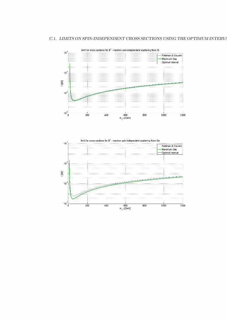
C.1. LIMITS ON SPIN-INDEPENDENT CROSS SECTIONS USING THE OPTIMUM INTERVAL METHOD139
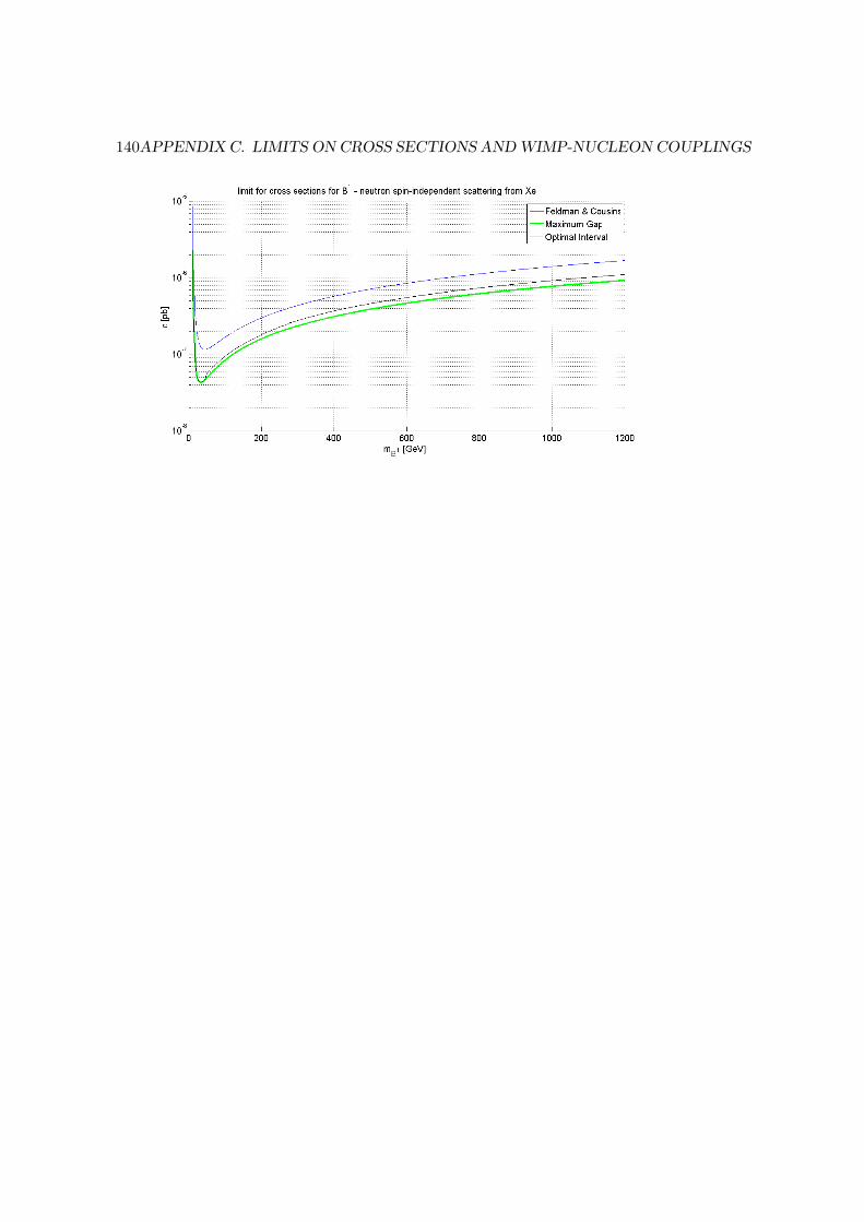
140APPENDIX C. LIMITS ON CROSS SECTIONS AND WIMP-NUCLEON COUPLINGS
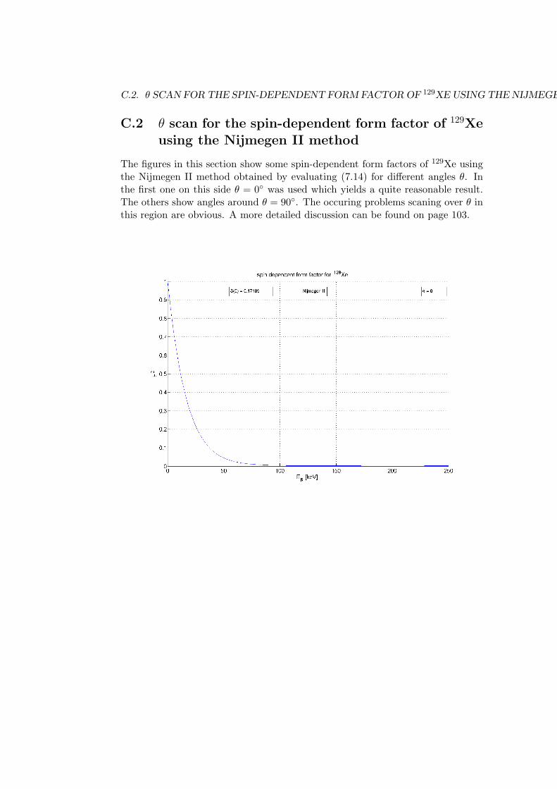
C.2. θ SCAN FOR THE SPIN-DEPENDENT FORM FACTOR OF 129XE USING THE NIJMEGEN II METHOD141
C.2 θ scan for the spin-dependent form factor of 129Xeusing the Nijmegen II method
The figures in this section show some spin-dependent form factors of 129Xe usingthe Nijmegen II method obtained by evaluating (7.14) for different angles θ. Inthe first one on this side θ = 0 was used which yields a quite reasonable result.The others show angles around θ = 90. The occuring problems scaning over θ inthis region are obvious. A more detailed discussion can be found on page 103.
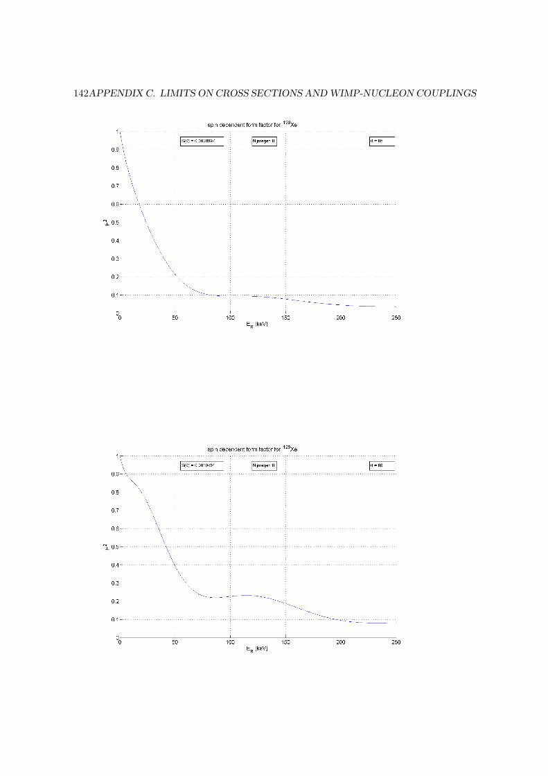
142APPENDIX C. LIMITS ON CROSS SECTIONS AND WIMP-NUCLEON COUPLINGS
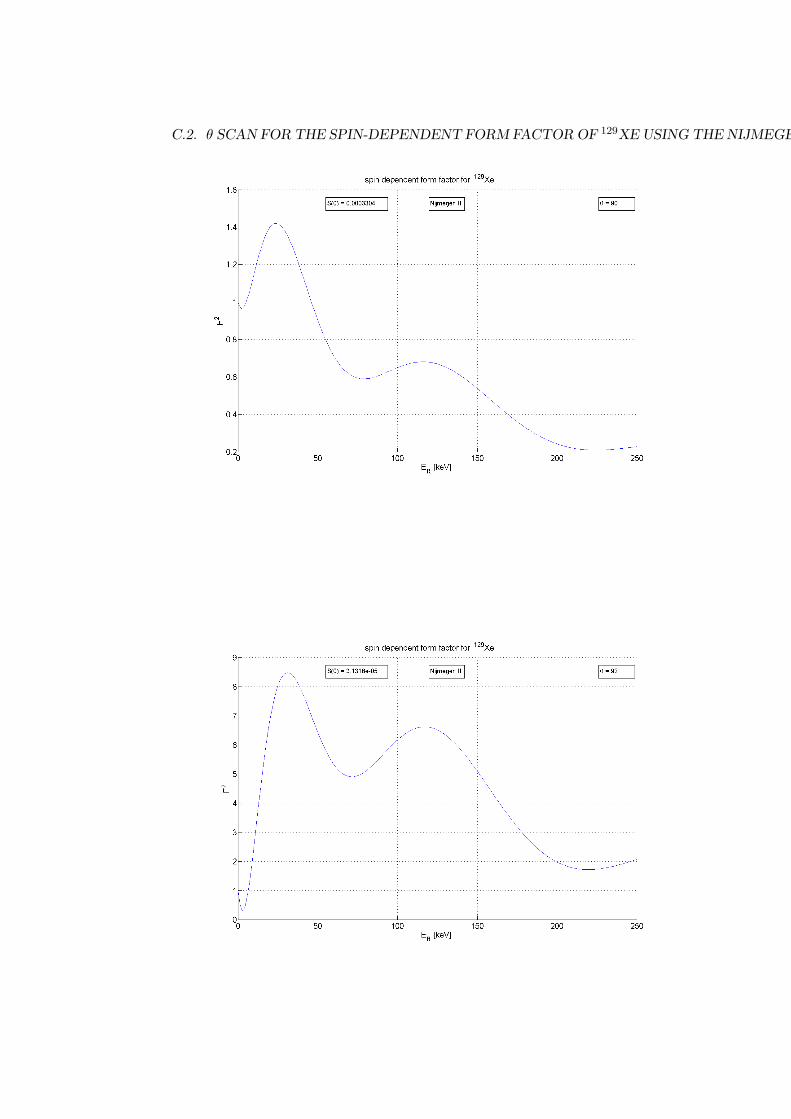
C.2. θ SCAN FOR THE SPIN-DEPENDENT FORM FACTOR OF 129XE USING THE NIJMEGEN II METHOD143
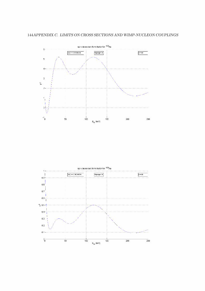
144APPENDIX C. LIMITS ON CROSS SECTIONS AND WIMP-NUCLEON COUPLINGS
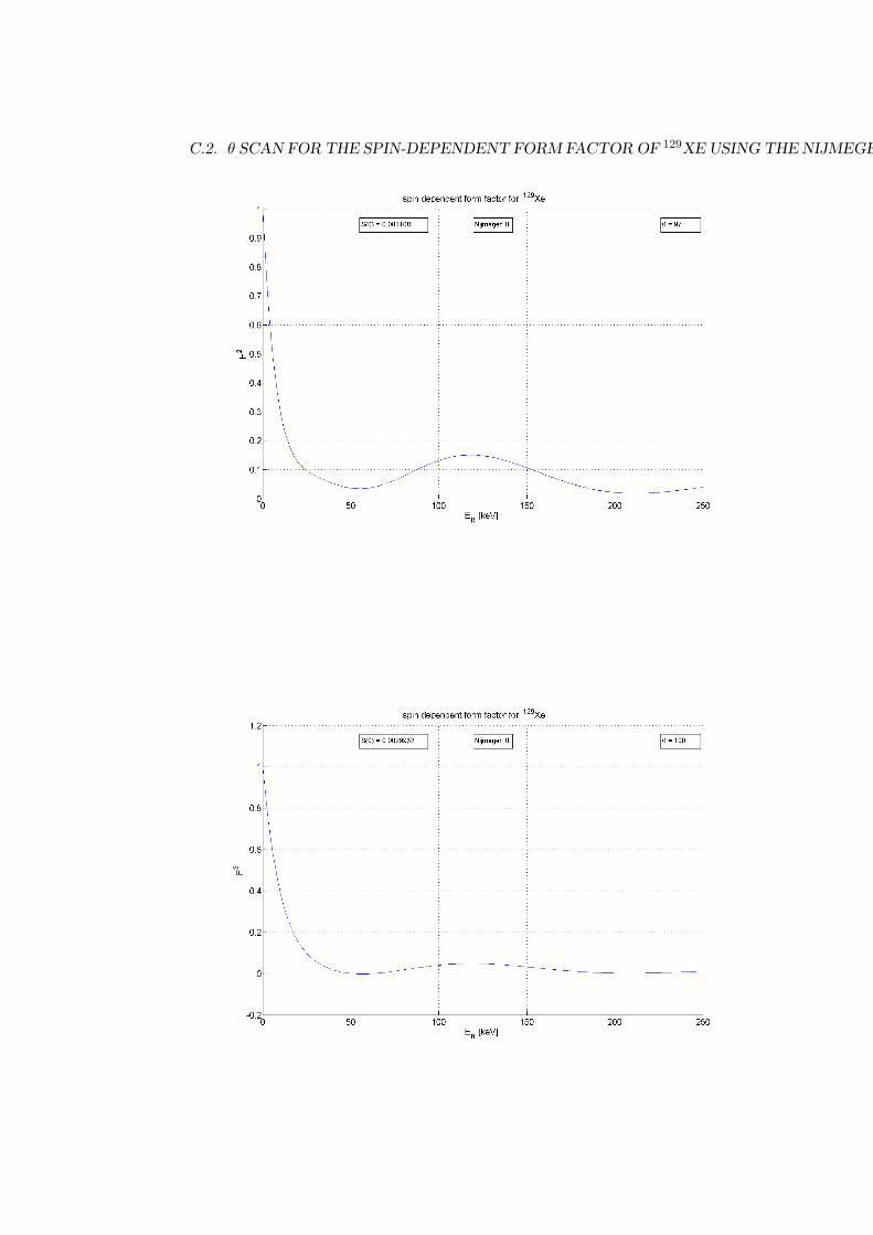
C.2. θ SCAN FOR THE SPIN-DEPENDENT FORM FACTOR OF 129XE USING THE NIJMEGEN II METHOD145
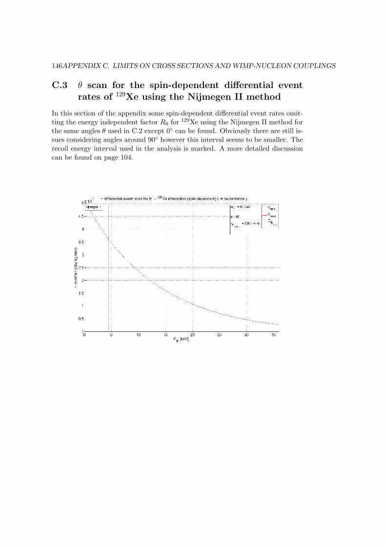
146APPENDIX C. LIMITS ON CROSS SECTIONS AND WIMP-NUCLEON COUPLINGS
C.3 θ scan for the spin-dependent differential eventrates of 129Xe using the Nijmegen II method
In this section of the appendix some spin-dependent differential event rates omit-ting the energy independent factor R0 for 129Xe using the Nijmegen II method forthe same angles θ used in C.2 except 0 can be found. Obviously there are still is-sues considering angles around 90 however this interval seems to be smaller. Therecoil energy interval used in the analysis is marked. A more detailed discussioncan be found on page 104.
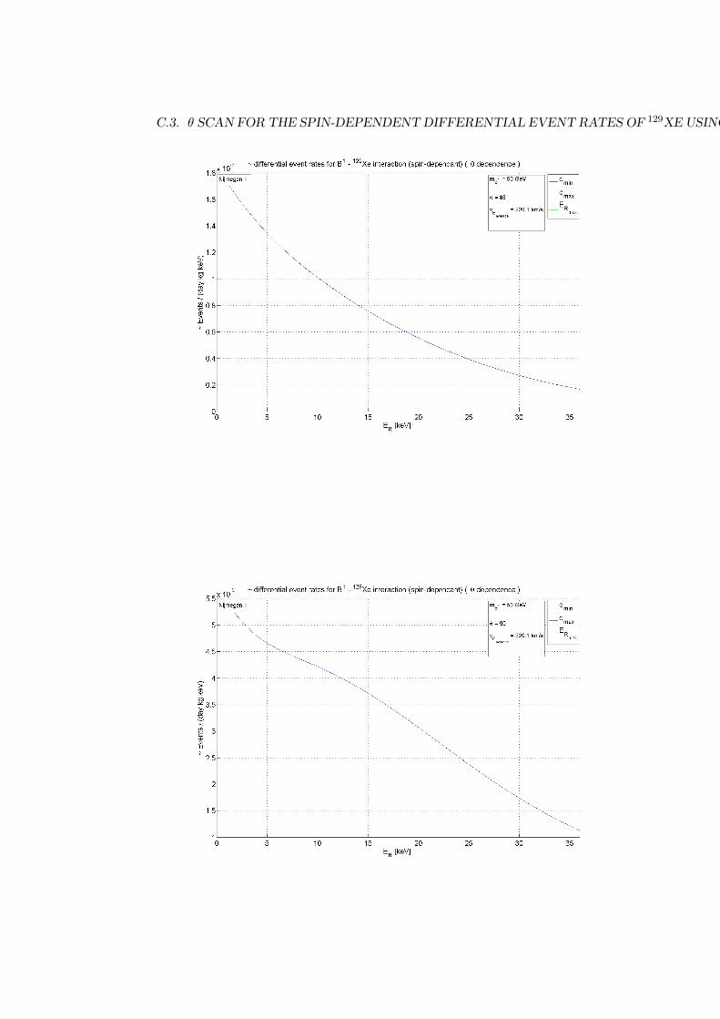
C.3. θ SCAN FOR THE SPIN-DEPENDENT DIFFERENTIAL EVENT RATES OF 129XE USING THE NIJMEGEN II METHOD147
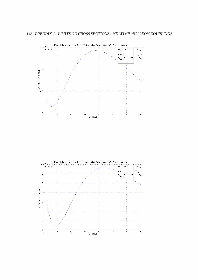
148APPENDIX C. LIMITS ON CROSS SECTIONS AND WIMP-NUCLEON COUPLINGS
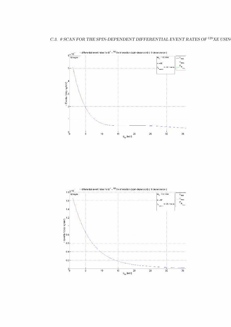
C.3. θ SCAN FOR THE SPIN-DEPENDENT DIFFERENTIAL EVENT RATES OF 129XE USING THE NIJMEGEN II METHOD149
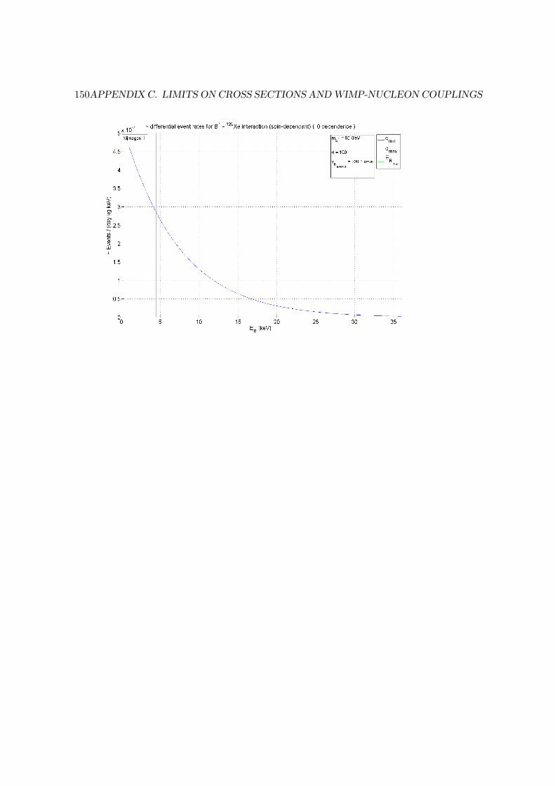
150APPENDIX C. LIMITS ON CROSS SECTIONS AND WIMP-NUCLEON COUPLINGS
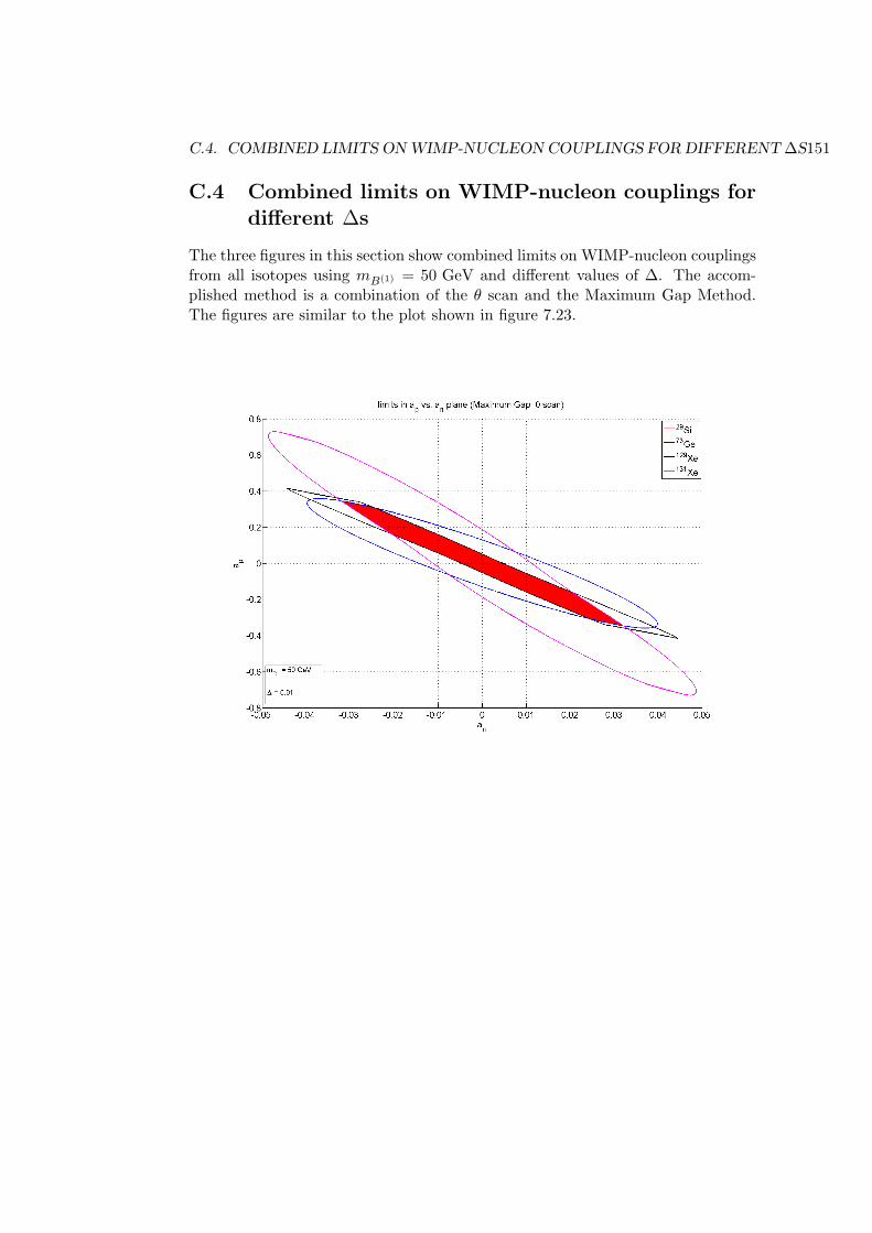
C.4. COMBINED LIMITS ON WIMP-NUCLEON COUPLINGS FOR DIFFERENT ∆S151
C.4 Combined limits on WIMP-nucleon couplings fordifferent ∆s
The three figures in this section show combined limits on WIMP-nucleon couplingsfrom all isotopes using mB(1) = 50 GeV and different values of ∆. The accom-plished method is a combination of the θ scan and the Maximum Gap Method.The figures are similar to the plot shown in figure 7.23.
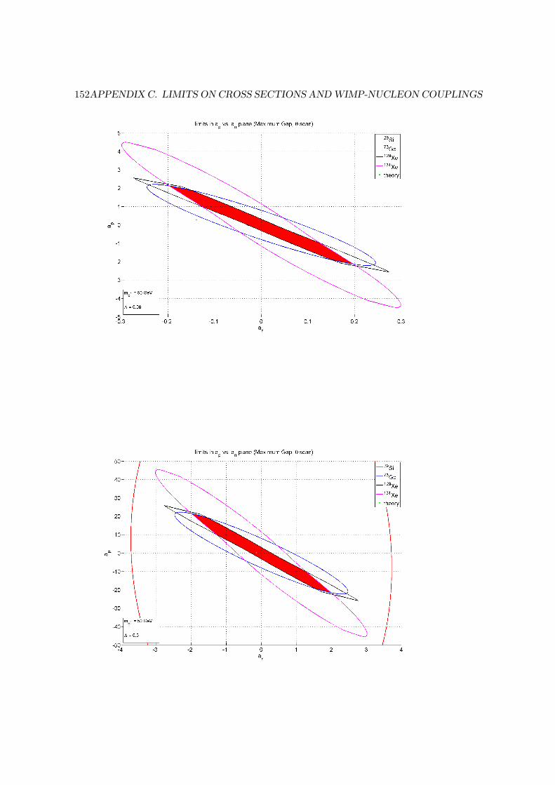
152APPENDIX C. LIMITS ON CROSS SECTIONS AND WIMP-NUCLEON COUPLINGS
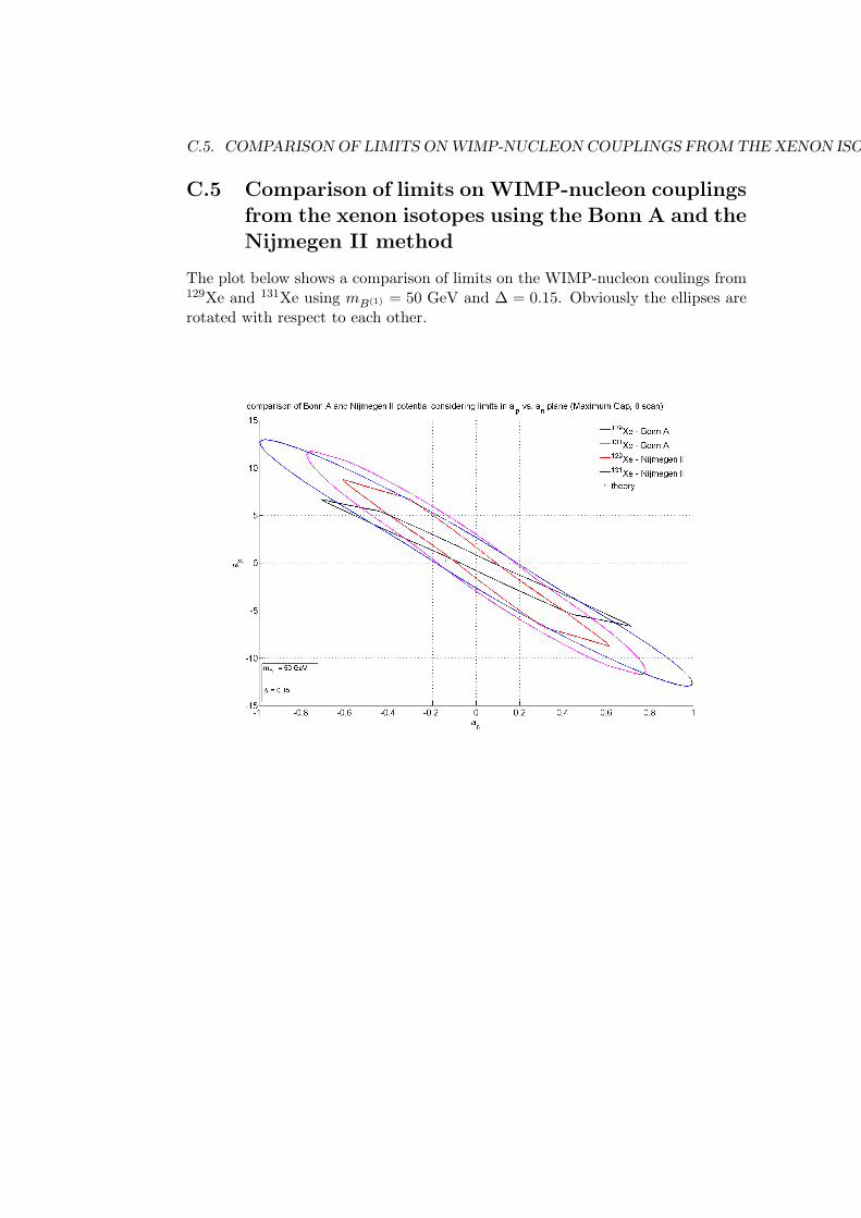
C.5. COMPARISON OF LIMITS ON WIMP-NUCLEON COUPLINGS FROM THE XENON ISOTOPES USING THE BONN A AND THE NIJMEGEN II METHOD153
C.5 Comparison of limits on WIMP-nucleon couplingsfrom the xenon isotopes using the Bonn A and theNijmegen II method
The plot below shows a comparison of limits on the WIMP-nucleon coulings from129Xe and 131Xe using mB(1) = 50 GeV and ∆ = 0.15. Obviously the ellipses arerotated with respect to each other.
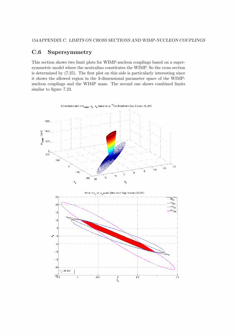
154APPENDIX C. LIMITS ON CROSS SECTIONS AND WIMP-NUCLEON COUPLINGS
C.6 Supersymmetry
This section shows two limit plots for WIMP-nucleon couplings based on a super-symmetric model where the neutralino constitutes the WIMP. So the cross sectionis determined by (7.25). The first plot on this side is particularly interesting sinceit shows the allowed region in the 3-dimensional parameter space of the WIMP-nucleon couplings and the WIMP mass. The second one shows combined limitssimilar to figure 7.23.
Bibliography
[1] T. Kaluza, Zum Unitatsproblem der Physik, Sitzungsber. Preuss. Akad.Wiss., Phys. Math. Kl. 966, 1921
[2] J. v. Dongen, Einstein and the Kaluza-Klein particle, arxiv:gr-qc/0009087
[3] L. O’Raifeartaigh, N. Strauman, Early history of Gauge Theoriesand Kaluza-Klein Theories, with a Glance at Recent Developments,arxiv:hep-ph/9810524
[4] O. Klein, Quantenthorie und funfdimensionale Relativitatstheorie, Z.Phys.37, 895, 1926
[5] K.R. Dienes, New directions for new dimensions: An introduction toKaluza-Klein theory, large extra dimensions and the brane world, 2002 TASIlectures
[6] D. Hooper, S. Profumo, Dark Matter and Collider Phenomenology of Uni-versal Extra Dimensions, arxiv:hep-ph/0701197
[7] G. D. Kribs, TASI 2004 Lectures on the Phenomenology of Extra Dimensions,arxiv:hep-ph/0605325
[8] T. Appelquist, H.-C. Cheng, B. A. Dobrescu, Bounds on Universal ExtraDimensions, arxiv:hep-ph/0012100
[9] H.-C. Cheng, K. T. Matchev, M. Schmaltz, Radiative Corrections to Kaluza-Klein Masses, arxiv:hep-ph/0204342
[10] G. Servant, T. M.P. Tait, Elastic Scattering and Direct Detection of Kaluza-Klein Dark Matter, arxiv:hep-ph/0209262
[11] D. N. Spergel et al., Wilkinson Microwave Anisotropy Probe (WMAP) ThreeYear Observations: Implications for Cosmology, arxiv:astro-ph/0603449
[12] K. Kong, K. T. Matchev, Precise Calculation of the Relic Density of Kaluza-Klein Dark Matter in Universal Extra Dimensions, arxiv:hep-ph/0509119
[13] J. Engel, S. Pittel, Nuclear Physics of Dark Matter Detection,Int. J. Mod. Phys. E Vol. 1 No. 1 (1992) 1-37
155
156 BIBLIOGRAPHY
[14] G. Jungman, M. Kamionkowski, K. Griest, Supersymmetric dark matter,Phys. Rept. 267 (1996)
[15] A. Kurylov, M. Kamionkowski, Generalized Analysis of Weakly-InteractingMassive Particle Searches, arxiv: hep-ph/0307185
[16] Particle Data Group, The Review of Particle Physics, http://pdg.lbl.gov
[17] H.-C. Cheng, J. L. Feng, K. T. Matchev, Kaluza-Klein Dark Matterarxiv:hep-ph/0207125
[18] D. Hooper, G. Zaharijas, Distinguishing Supersymmetry From UniversalExtra Dimensions or Little Higgs Models With Dark Matter Experiments,arxiv:hep-ph/0612137
[19] L. Baudis, The XENON10 WIMP Search Experiment at the Gran SassoUnderground Laboratory, arxiv:astrp-ph/0703183
[20] J. Angle et al., First Results from the XENON10 Dark Matter Experimentat the Gran Sasso National Laboratory, arxiv:/0706.0039
[21] http://webelements.com/
[22] V. A. Bednyakov, F. Simkovic, Nuclear spin structure in dark matter search:The zero momentum transfer limit, arxiv:/hep-ph/0406218
[23] V. A. Bednyakov, F. Simkovic, Nuclear spin structure in dark matter search:The finite momentum transfer limit, arxiv:/hep-ph/0608097
[24] J. D. Lewin, P. F. Smith, Review of mathematics, numerical factors andcorrections for Dark Matter experiments based on elastic nuclear recoil, As-tropart. Phys. 6, 87 (1996)
[25] R. H. Helm, Phys. Rev. 104 (1956) 1466
[26] M. T. Ressell et al., Nuclear shell model calculations of neutralino-nucleuscross sections for 29Si and 73Ge, Phys. Rev. D 48 5519 (1993)
[27] V. Dimitrov, J. Engel, S. Pittel, Scattering of weakly interacting massiveparticles from 73Ge, arxiv:/hep-ph/9408246
[28] M. T. Ressell, D. J. Dean, Spin-Dependent Neutralino-Nucleus Scattering forA ∼ 127 Nuclei, arxiv:/hep-ph/9702290
[29] J. Engel, Nuclear form factors for the scattering of weakly interacting massiveparticles, Phys. Lett. B 264 114 (1991)
[30] J. D. Vergados, On the Direct Detection of Dark Matter - Exploring all thesignatures of the neutralino-nucleus interaction, arxiv:/hep-ph/0601064
BIBLIOGRAPHY 157
[31] D. S. Akerib et al., Exclusion limits on the WIMP-Nucleon Cross-Sectionfrom the First Run of the Cryogenic Dark Matter Search in the SoudanUnderground Lab, arxiv:/astro-ph/0507190
[32] D. S. Akerib et al., Limits on spin-independent WIMP-nucleon inter-actions from the two-tower run of the Cryogenic Dark Matter Search,arxiv:/astro-ph/0509259
[33] M. C. Smith et. al, The RAVE Survey: Constraining the Local GalacticEscape Speed, arxiv:/astro-ph/0611671
[34] E. I. Gates, G. Gyuk, M. S. Turner, The local halo density,arxiv:/astro-ph/9505039
[35] M. J. Lewis, K. Freese, The Phase of the Annual Modulation: Constrainingthe WIMP mass, arxiv:/astro-ph/0307190
[36] F. Giuliani, Are Direct Search Experiments Sensitive to All Spin-IndependentWeakly Interacting Massive Particles?, arxiv:/hep-ph/0504157
[37] G. J. Feldman, R. D. Cousins, Unified approach to the classical statisticalanalysis of small signals, Phys. Rev. D 57, 3873 (1998)
[38] S. Yellin, Finding an upper limit in the presence of an unknown background,Phys. Rev. D 66, 032005 (2002)
[39] http://titus.stanford.edu/Upperlimit/
[40] C. Savage, P. Gondolo, K. Freese, Can WIMP Spin Dependent Couplingsexplain DAMA data in the light of Null Results from Other Experiments?,arxiv:/astro-ph/0408346
[41] D. R. Tovey et al., A New Model-Independent Method for Extract-ing Spin-Dependent Cross Section limits from Dark Matter Searches,arxiv:/hep-ph/0005041
[42] G. J. Alner et al. Limits on spin-dependent WIMP-nucleon cross-sectionsfrom the first ZEPLIN-II data, arxiv:/0708.1883
Acknowledgement
Hiermit mochte ich mich bei einigen Menschen bedanken, die entscheidend bei derDurchfuhrung dieser Arbeit geholfen haben. Zunachst mochte ich dabei naturlichLaura danken, insbesondere auch dafur, dass ich in Zurich meine Doktorarbeitmachen kann. Desweiteren danke ich meinen Burokollegen Stefan, Tobi undMichael fur ein sehr interessantes Jahr. Abgesehen davon naturlich meiner Mutter,Jihye und schliesslich Ssico.
158
Statement
Hiermit versichere ich, dass ich die vorliegende Arbeit selbststandig und ohneBenutzung anderer als der angegebenen Quellen und Hilfsmittel angefertigt habe.Aachen, den 02. Oktober 2007
159


![Kaluza-Klein Theories - basic idea · Kaluza-Klein Theories - basic idea. 34 CHAPTER 3. EXTRA SPATIAL DIMENSIONS Figure 3.2: (Taken from [46]). The full spectrum of the UED model](https://img.pdfslide.net/doc/110x75/5c753c5d09d3f287228c576b/kaluza-klein-theories-basic-idea-kaluza-klein-theories-basic-idea-34-chapter.jpg)