Supermodularity is not Falsifiable∗

Christopher P. Chambers and Federico Echenique †

May 18, 2006

Abstract

Supermodularity has long been regarded as a natural notion ofcomplementarities in individual decision making; it was introducedas such in the nineteenth century by Edgeworth and Pareto. Butsupermodularity is not an ordinal property. We study the ordinalcontent of assuming a supermodular utility, i.e. what it means for theindividual’s underlying preferences. We show that supermodularityis a very weak property, in the sense that many preferences have asupermodular representation. As a consequence, supermodularity isnot testable using data on individual consumption. We also studysupermodularity in the Choquet expected utility model, and showthat uncertainty aversion is generally not testable when only bets areobserved.

JEL Classification: D11,D24,C78Keywords: Supermodular Function, Quasisupermodularity, Complementari-ties, Afriat’s model, Uncertainty Aversion, Choquet expected utility.

∗We are specially grateful to Chris Shannon for comments and suggestions on a previousdraft. We also thank PJ Healy, Laurent Mathevet, Preston McAfee, Ed Schlee, YvesSprumont, Leeat Yariv, Bill Zame and seminar participants in UC Berkeley, UC Davis,USC, and the 2006 Southwest Economic Theory Conference.

†Division of the Humanities and Social Sciences, California Institute of Technol-ogy, Pasadena CA 91125, USA. Email: chambers@hss.caltech.edu (Chambers) andfede@hss.caltech.edu (Echenique)

1

1 Introduction

Economists have long regarded supermodularity as the formal expression

of complementarity in preference; according to Samuelson (1947), the use

of supermodularity as a notion of complementarities dates back to Fischer,

Pareto and Edgeworth. Our goal in this paper is to show that this approach

is misguided by establishing that the assumption of supermodularity lacks

empirical content in many ordinal economic models.

Supermodularity is a cardinal property of a function defined on a lattice.

It roughly states that a function has “increasing differences.” For this rea-

son, it is usually interpreted as modeling complementarities. For example,

consider a consumer with a utility function over two goods. A natural notion

of complementarity is that the two goods are complementary if the marginal

utility of consuming one of the goods is increasing in the consumption of the

other; for smooth functions, if the cross-partial derivatives are non-negative.

This notion is equivalent to supermodularity of the utility function.

Because it is a cardinal property, a number of authors, including Allen

(1934), Hicks and Allen (1934), Samuelson (1947), and Stigler (1950), have al-

ready rejected supermodularity as a notion of complementarities (see Samuel-

son (1974) for a summary of the historical debate). They thought that, be-

cause it is a cardinal and not an ordinal notion, it would have no testable

implications. While these authors had intuitively the right idea, their ar-

gument was incomplete. Their argument ran as follows: A supermodular

function has positive cross-derivatives. Fix any given point. We may take an

ordinal transformation of the function, preserving the preferences it repre-

sents, such that some cross-derivatives at this point become negative. While

this is correct, it only demonstrates the lack of testable implications of su-

permodularity as a local property. Supermodularity at any given point (in

2

the form of nonnegative cross-derivatives) is not refutable. However, they

believed that, as a consequence, supermodularity has no global implications.

The argument in Samuelson, Hicks, Allen and Stigler is weak, as local

violations of supermodularity have no obvious consequences for consumer

behavior. More importantly, they were incorrect in believing that super-

modularity has no ordinal implications. In an influential paper, Milgrom and

Shannon (1994) introduced quasisupermodularity, an ordinal implication of

supermodularity. Thus, when one assumes a function is supermodular, one is

also making the assumption that the preference represented by this function

is quasisupermodular.

Milgrom and Shannon characterized quasisupermodular functions as a

class of functions with a monotone comparative statics property. Quasisu-

permodularity is a strict generalization of the concept of supermodularity,

in the sense that there exist quasisupermodular preferences which cannot

be represented by supermodular utility functions. Nevertheless, supermod-

ularity has dominated quasisupermodularity as an assumption in economic

applications. This is true even in the case where the function assumed to

be supermodular has only ordinal significance. Our work should help to

understand why this is the case.

Our main results will characterize the ordinal content of supermodularity

and show that, in many situations, it is equivalent to quasisupermodularity.

We show that supermodularity has few empirical implications for general

individual decision-making environments, and no implications for data on

consumption decisions, thus rigorously confirming the intuition of Samuelson,

Hicks, Allen and Stigler’s.

Consider a consumer with preferences over a finite set of consumption

bundles. We characterize the preferences that can be represented by a super-

3

modular utility function. Our primary result shows that weakly increasing

and quasisupermodular preferences which are representable can be repre-

sented by a supermodular utility function. We also show a dual statement,

that weakly decreasing, quasisupermodular and representable preferences

have a supermodular representation. Thus, for many economic applications

(where there is free disposal, or scarcity is modeled by monotonicity of prefer-

ence relations), assuming an agent has a supermodular utility is no stronger

than assuming his preference is quasisupermodular.

If quasisupermodularity is an ordinal implication of supermodularity, how

can one make the claim that supermodularity is not falsifiable? The answer is

simple: any strictly monotonic function is automatically quasisupermodular.

So our results imply that any consumer with strictly increasing preferences

can be modeled as having a supermodular utility function. This suggests that

supermodularity may not be an appropriate mathematical interpretation of

the notion of complementarity, as it is implied by selfish behavior alone.

We also fully characterize the class of all preferences (monotonic or other-

wise) which can be represented by a supermodular utility; in this sense we are

the first to establish the ordinal content of assuming supermodularity. We

present an analogous characterization of quasisupermodularity, and compare

it with the characterization of supermodularity.

Our results have direct and negative implications for the refutability of

supermodularity in economic environments. We present these implications

for two models: Afriat’s model of consumption data and Schmeidler’s model

of uncertainty aversion.

First, we consider Afriat’s (1967) model of data generated by an indi-

vidual choosing consumption bundles at different prices. Arguably, this is

the right model for the question of whether supermodularity has empirical

4

implications in consumer theory. We show that the choices are either irra-

tional, and cannot be rationalized by any utility function, or they can be

rationalized by a supermodular utility function. Our result is reminiscent

of Afriat’s (1967) (see also Varian (1982)) finding that the concavity of util-

ity functions has no testable implications; we find that supermodularity has

no testable implications. In addition, we investigate the joint assumption

of supermodularity and concavity. We show that the joint assumption has

testable implications by presenting an example that can be rationalized by

a supermodular and by a concave utility, but not by a utility with both

properties.

Its lack of testable implications is further evidence that supermodularity

is problematic as a notion of complementarity in consumption. Our finding

is, in a sense, more problematic than Afriat’s was for concavity, because one

possible interpretation of concavity is as an implication of risk-aversion, and

as such it is testable using lotteries. The interpretation of supermodularity

as complementarity suggests statements about a consumer choosing—to use

a textbook example—coffee and sugar. For such environments, we show that

supermodularity is vacuous.

Our second application is to decision-making under uncertainty. Super-

modularity is used to model uncertainty aversion in the Choquet expected

utility model (Schmeidler, 1989). We study the refutability of uncertainty

aversion when observing preferences over binary acts (bets) alone. We show

that in many situations, uncertainty aversion has no testable implications.

In particular, uncertainty aversion is not refutable using data on choices over

binary acts when any event is considered more likely than any subevent. It is

only refutable using data on more complicated acts, but such acts also entail

attitudes towards risk.

5

Do our results imply that supermodularity is completely useless and has

no place in economic theory? The answer is clearly no. Supermodularity has

proved a useful assumption in very different areas in economics. It has been

useful because it has strong theoretical implications.1 But the environments

in which supermodularity is useful are usually cardinal environments. To

illustrate this, let us consider two examples.

First, in Becker’s (1973)’s marriage market model, there are two types

of agents, say, men and women. Men and women are ordered according to

some characteristic, say height. When a man matches to a woman, they

generate some numerical surplus. Becker assumes that this surplus function

is supermodular in height: thus, the extra surplus generated when a given

man matches with a taller woman is higher for a taller man. Becker’s primary

interest is in maximizing the aggregate surplus of a given matching. Becker

shows that the matchings which maximize aggregate surplus are assortative:

the tallest man is matched with the tallest woman, and so forth, in decreasing

order. One might be tempted to think that our results therefore imply that

any increasing surplus function leads to assortative matchings. However, this

conclusion is incorrect. The matching-maximizing aggregate surplus is not

preserved under arbitrary ordinal transformation. In Becker’s model, the

surplus is cardinally measurable and freely transferable.

Another model in which supermodularity proves extremely useful is in

the theory of transferable-utility games. Shapley (1971) showed that any

transferable-utility game which is supermodular has a nonempty core. Are we

to therefore conclude that any game which is strictly monotonic (and can be

ordinally transformed into a supermodular game) also has a nonempty core?

Obviously not. Again, the solution concept of the core is a cardinal con-

1See the books by Topkis (1998) and Vives (1999) and the recent survey by Vives(2005).

6

cept, and the core is obviously not preserved under ordinal transformations.

Hence, there are important economic applications in which supermodularity

is meaningful and has implications.

We should also emphasize that the joint assumption of supermodularity

and other properties can also have implications. Chipman (1977) showed that

a differentiable, strongly concave and supermodular utility implies a normal

demand. Quah (2004) shows that a concave and supermodular utility im-

plies a class of monotone comparative statics; among other results, Quah

generalizes Chipman’s theorem. It seems important to study the testable

implications of the joint assumptions of supermodularity and concavity. Nei-

ther our nor Afriat’s results give an answer to this problem. The problem is

that Afriat’s separation argument is in the so-called “Afriat numbers,” while

ours is in the utility indexes themselves. However, two recent papers, one

by Richter and Wong (2004), the other by Kannai (2005), state necessary

and sufficient conditions for an order on a finite subset of some Euclidean

space to be representable by a concave function. It is possible that combining

their condition with ours in some way will lead to a necessary and sufficient

condition for supermodular and concave representation.

We comment on the existing results that are related to ours.

Li Calzi (1990) presents classes of functions f such that a continuous in-

creasing transformation of f is supermodular. He is also the first to note a

connection between monotonicity and supermodularity, although his frame-

work is different. While we establish our results for binary relations on a finite

lattice, he shows that any twice differentiable strictly increasing function on

a compact product lattice in Rn is ordinally equivalent to a supermodular

function. Li Calzi does not study the testability of supermodularity (but see

the comment in Section 6 on how his results can be used).

7

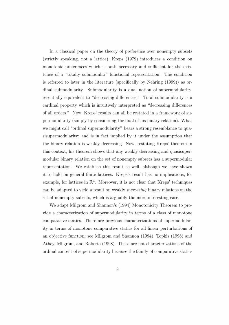
In a classical paper on the theory of preference over nonempty subsets

(strictly speaking, not a lattice), Kreps (1979) introduces a condition on

monotonic preferences which is both necessary and sufficient for the exis-

tence of a “totally submodular” functional representation. The condition

is referred to later in the literature (specifically by Nehring (1999)) as or-

dinal submodularity. Submodularity is a dual notion of supermodularity,

essentially equivalent to “decreasing differences.” Total submodularity is a

cardinal property which is intuitively interpreted as “decreasing differences

of all orders.” Now, Kreps’ results can all be restated in a framework of su-

permodularity (simply by considering the dual of his binary relation). What

we might call “ordinal supermodularity” bears a strong resemblance to qua-

sisupermodularity; and is in fact implied by it under the assumption that

the binary relation is weakly decreasing. Now, restating Kreps’ theorem in

this context, his theorem shows that any weakly decreasing and quasisuper-

modular binary relation on the set of nonempty subsets has a supermodular

representation. We establish this result as well, although we have shown

it to hold on general finite lattices. Kreps’s result has no implications, for

example, for lattices in Rn. Moreover, it is not clear that Kreps’ techniques

can be adapted to yield a result on weakly increasing binary relations on the

set of nonempty subsets, which is arguably the more interesting case.

We adapt Milgrom and Shannon’s (1994) Monotonicity Theorem to pro-

vide a characterization of supermodularity in terms of a class of monotone

comparative statics. There are previous characterizations of supermodular-

ity in terms of monotone comparative statics for all linear perturbations of

an objective function; see Milgrom and Shannon (1994), Topkis (1998) and

Athey, Milgrom, and Roberts (1998). These are not characterizations of the

ordinal content of supermodularity because the family of comparative statics

8

is obtained by linear perturbations.

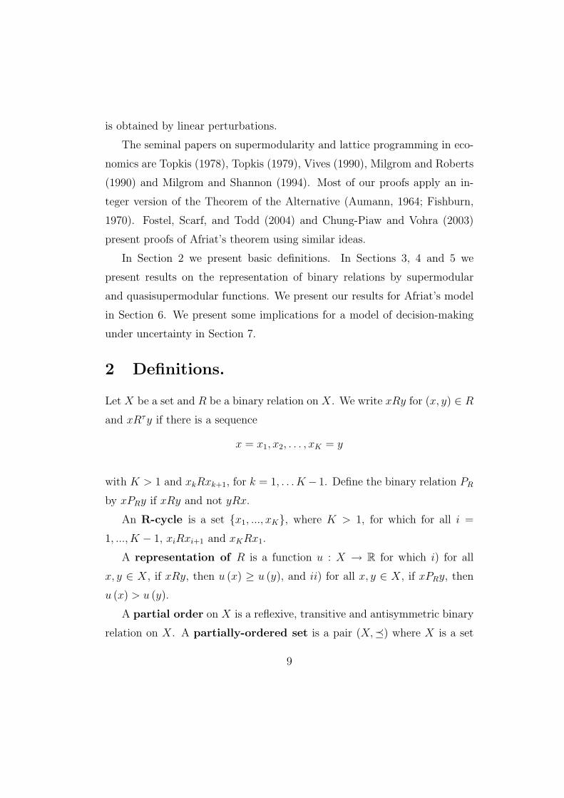
The seminal papers on supermodularity and lattice programming in eco-

nomics are Topkis (1978), Topkis (1979), Vives (1990), Milgrom and Roberts

(1990) and Milgrom and Shannon (1994). Most of our proofs apply an in-

teger version of the Theorem of the Alternative (Aumann, 1964; Fishburn,

1970). Fostel, Scarf, and Todd (2004) and Chung-Piaw and Vohra (2003)

present proofs of Afriat’s theorem using similar ideas.

In Section 2 we present basic definitions. In Sections 3, 4 and 5 we

present results on the representation of binary relations by supermodular

and quasisupermodular functions. We present our results for Afriat’s model

in Section 6. We present some implications for a model of decision-making

under uncertainty in Section 7.

2 Definitions.

Let X be a set and R be a binary relation on X. We write xRy for (x, y) ∈ R

and xRτy if there is a sequence

x = x1, x2, . . . , xK = y

with K > 1 and xkRxk+1, for k = 1, . . . K− 1. Define the binary relation PR

by xPRy if xRy and not yRx.

An R-cycle is a set x1, ..., xK, where K > 1, for which for all i =

1, ..., K − 1, xiRxi+1 and xKRx1.

A representation of R is a function u : X → R for which i) for all

x, y ∈ X, if xRy, then u (x) ≥ u (y), and ii) for all x, y ∈ X, if xPRy, then

u (x) > u (y).

A partial order on X is a reflexive, transitive and antisymmetric binary

relation on X. A partially-ordered set is a pair (X,) where X is a set

9

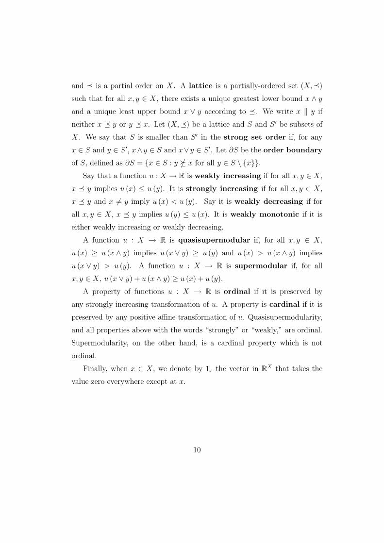
and is a partial order on X. A lattice is a partially-ordered set (X,)

such that for all x, y ∈ X, there exists a unique greatest lower bound x ∧ y

and a unique least upper bound x ∨ y according to . We write x ‖ y if

neither x y or y x. Let (X,) be a lattice and S and S ′ be subsets of

X. We say that S is smaller than S ′ in the strong set order if, for any

x ∈ S and y ∈ S ′, x∧y ∈ S and x∨y ∈ S ′. Let ∂S be the order boundary

of S, defined as ∂S = x ∈ S : y x for all y ∈ S \ x.Say that a function u : X → R is weakly increasing if for all x, y ∈ X,

x y implies u (x) ≤ u (y). It is strongly increasing if for all x, y ∈ X,

x y and x 6= y imply u (x) < u (y). Say it is weakly decreasing if for

all x, y ∈ X, x y implies u (y) ≤ u (x). It is weakly monotonic if it is

either weakly increasing or weakly decreasing.

A function u : X → R is quasisupermodular if, for all x, y ∈ X,

u (x) ≥ u (x ∧ y) implies u (x ∨ y) ≥ u (y) and u (x) > u (x ∧ y) implies

u (x ∨ y) > u (y). A function u : X → R is supermodular if, for all

x, y ∈ X, u (x ∨ y) + u (x ∧ y) ≥ u (x) + u (y).

A property of functions u : X → R is ordinal if it is preserved by

any strongly increasing transformation of u. A property is cardinal if it is

preserved by any positive affine transformation of u. Quasisupermodularity,

and all properties above with the words “strongly” or “weakly,” are ordinal.

Supermodularity, on the other hand, is a cardinal property which is not

ordinal.

Finally, when x ∈ X, we denote by 1x the vector in RX that takes the

value zero everywhere except at x.

10

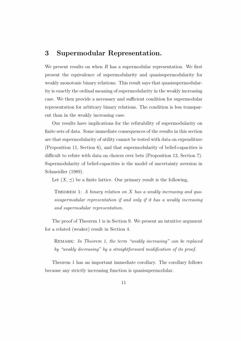
3 Supermodular Representation.

We present results on when R has a supermodular representation. We first

present the equivalence of supermodularity and quasisupermodularity for

weakly monotonic binary relations. This result says that quasisupermodular-

ity is exactly the ordinal meaning of supermodularity in the weakly increasing

case. We then provide a necessary and sufficient condition for supermodular

representation for arbitrary binary relations. The condition is less transpar-

ent than in the weakly increasing case.

Our results have implications for the refutability of supermodularity on

finite sets of data. Some immediate consequences of the results in this section

are that supermodularity of utility cannot be tested with data on expenditure

(Proposition 11, Section 6), and that supermodularity of belief-capacities is

difficult to refute with data on choices over bets (Proposition 13, Section 7).

Supermodularity of belief-capacities is the model of uncertainty aversion in

Schmeidler (1989).

Let (X,) be a finite lattice. Our primary result is the following,

Theorem 1: A binary relation on X has a weakly increasing and qua-

sisupermodular representation if and only if it has a weakly increasing

and supermodular representation.

The proof of Theorem 1 is in Section 9. We present an intuitive argument

for a related (weaker) result in Section 4.

Remark: In Theorem 1, the term “weakly increasing” can be replaced

by “weakly decreasing” by a straightforward modification of its proof.

Theorem 1 has an important immediate corollary. The corollary follows

because any strictly increasing function is quasisupermodular.

11

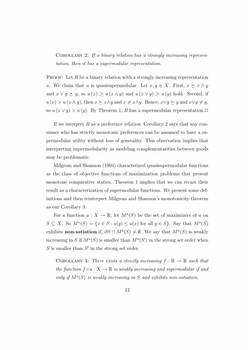
Corollary 2: If a binary relation has a strongly increasing represen-

tation, then it has a supermodular representation.

Proof: Let R be a binary relation with a strongly increasing representation

u. We claim that u is quasisupermodular. Let x, y ∈ X. First, x x ∧ y

and x ∨ y y, so u (x) ≥ u (x ∧ y) and u (x ∨ y) ≥ u (y) hold. Second, if

u (x) > u (x ∧ y), then x x∧y and x 6= x∧y. Hence, x∨y y and x∨y 6= y,

so u (x ∨ y) > u (y). By Theorem 1, R has a supermodular representation.2

If we interpret R as a preference relation, Corollary 2 says that any con-

sumer who has strictly monotonic preferences can be assumed to have a su-

permodular utility without loss of generality. This observation implies that

interpreting supermodularity as modeling complementarities between goods

may be problematic.

Milgrom and Shannon (1994) characterized quasisupermodular functions

as the class of objective functions of maximization problems that present

monotone comparative statics. Theorem 1 implies that we can recast their

result as a characterization of supermodular functions. We present some def-

initions and then reinterpret Milgrom and Shannon’s monotonicity theorem

as our Corollary 3.

For a function u : X → R, let Mu(S) be the set of maximizers of u on

S ⊆ X. So Mu(S) = x ∈ S : u(y) ≤ u(x) for all y ∈ S. Say that Mu(S)

exhibits non-satiation if, ∂S ∩ Mu(S) 6= ∅. We say that Mu(S) is weakly

increasing in S if Mu(S) is smaller than Mu(S ′) in the strong set order when

S is smaller than S ′ in the strong set order.

Corollary 3: There exists a strictly increasing f : R → R such that

the function f u : X → R is weakly increasing and supermodular if and

only if Mu(S) is weakly increasing in S and exhibits non-satiation.

12

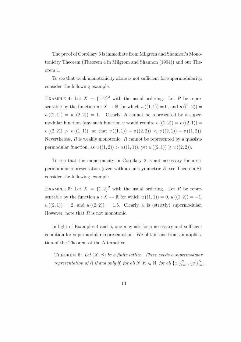
The proof of Corollary 3 is immediate from Milgrom and Shannon’s Mono-

tonicity Theorem (Theorem 4 in Milgrom and Shannon (1994)) and our The-

orem 1.

To see that weak monotonicity alone is not sufficient for supermodularity,

consider the following example.

Example 4: Let X = 1, 22 with the usual ordering. Let R be repre-

sentable by the function u : X → R for which u ((1, 1)) = 0, and u ((1, 2)) =

u ((2, 1)) = u ((2, 2)) = 1. Clearly, R cannot be represented by a super-

modular function (any such function v would require v ((1, 2)) = v ((2, 1)) =

v ((2, 2)) > v ((1, 1)), so that v ((1, 1)) + v ((2, 2)) < v ((2, 1)) + v ((1, 2)).

Nevertheless, R is weakly monotonic. R cannot be represented by a quasisu-

permodular function, as u ((1, 2)) > u ((1, 1)), yet u ((2, 1)) ≥ u ((2, 2)).

To see that the monotonicity in Corollary 2 is not necessary for a su-

permodular representation (even with an antisymmetric R, see Theorem 8),

consider the following example.

Example 5: Let X = 1, 22 with the usual ordering. Let R be repre-

sentable by the function u : X → R for which u ((1, 1)) = 0, u ((1, 2)) = −1,

u ((2, 1)) = 2, and u ((2, 2)) = 1.5. Clearly, u is (strictly) supermodular.

However, note that R is not monotonic.

In light of Examples 4 and 5, one may ask for a necessary and sufficient

condition for supermodular representation. We obtain one from an applica-

tion of the Theorem of the Alternative.

Theorem 6: Let (X,) be a finite lattice. There exists a supermodular

representation of R if and only if, for all N, K ∈ N, for all xiNi=1 , yiN

i=1,

13

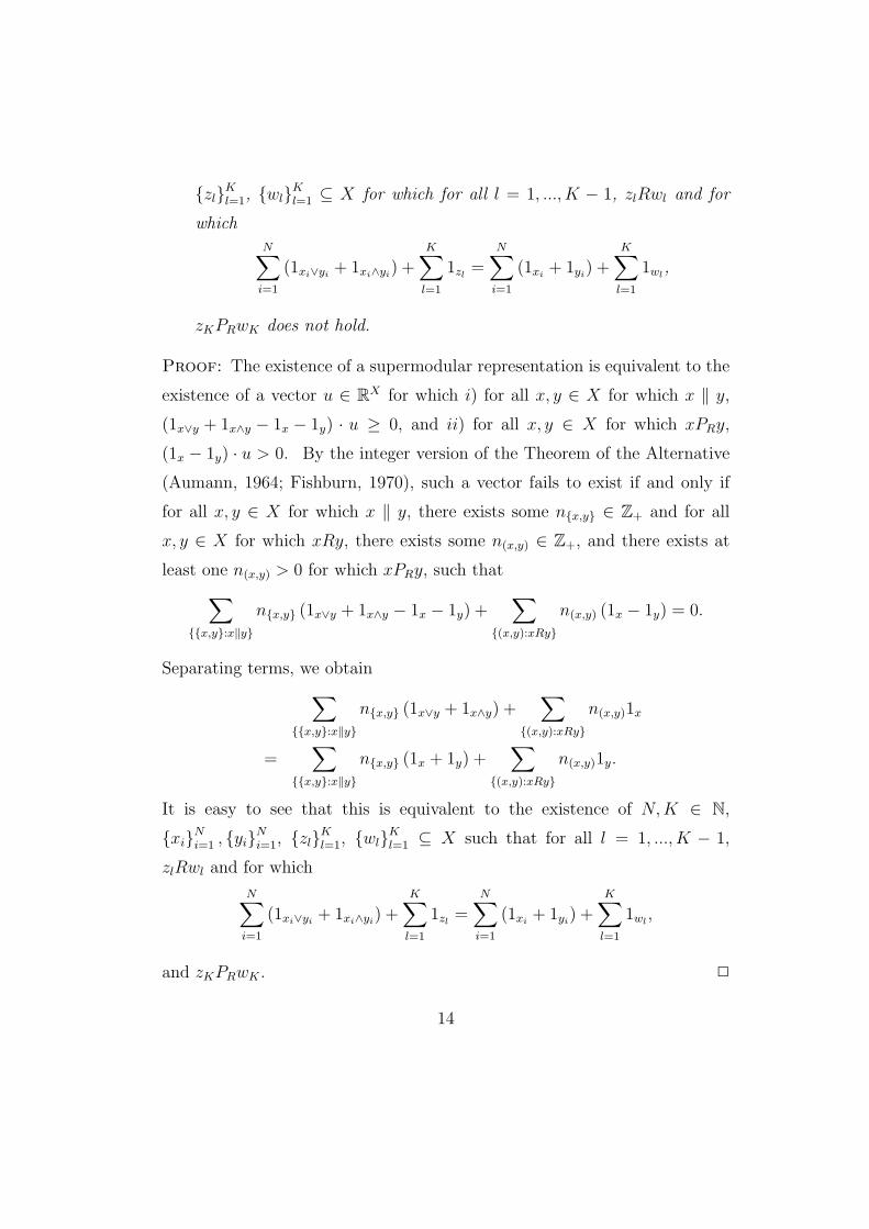
zlKl=1, wlK

l=1 ⊆ X for which for all l = 1, ..., K − 1, zlRwl and for

which

N∑i=1

(1xi∨yi+ 1xi∧yi

) +K∑

l=1

1zl=

N∑i=1

(1xi+ 1yi

) +K∑

l=1

1wl,

zKPRwK does not hold.

Proof: The existence of a supermodular representation is equivalent to the

existence of a vector u ∈ RX for which i) for all x, y ∈ X for which x ‖ y,

(1x∨y + 1x∧y − 1x − 1y) · u ≥ 0, and ii) for all x, y ∈ X for which xPRy,

(1x − 1y) · u > 0. By the integer version of the Theorem of the Alternative

(Aumann, 1964; Fishburn, 1970), such a vector fails to exist if and only if

for all x, y ∈ X for which x ‖ y, there exists some nx,y ∈ Z+ and for all

x, y ∈ X for which xRy, there exists some n(x,y) ∈ Z+, and there exists at

least one n(x,y) > 0 for which xPRy, such that∑x,y:x‖y

nx,y (1x∨y + 1x∧y − 1x − 1y) +∑

(x,y):xRy

n(x,y) (1x − 1y) = 0.

Separating terms, we obtain∑x,y:x‖y

nx,y (1x∨y + 1x∧y) +∑

(x,y):xRy

n(x,y)1x

=∑

x,y:x‖y

nx,y (1x + 1y) +∑

(x,y):xRy

n(x,y)1y.

It is easy to see that this is equivalent to the existence of N, K ∈ N,

xiNi=1 , yiN

i=1, zlKl=1, wlK

l=1 ⊆ X such that for all l = 1, ..., K − 1,

zlRwl and for which

N∑i=1

(1xi∨yi+ 1xi∧yi

) +K∑

l=1

1zl=

N∑i=1

(1xi+ 1yi

) +K∑

l=1

1wl,

and zKPRwK . 2

14

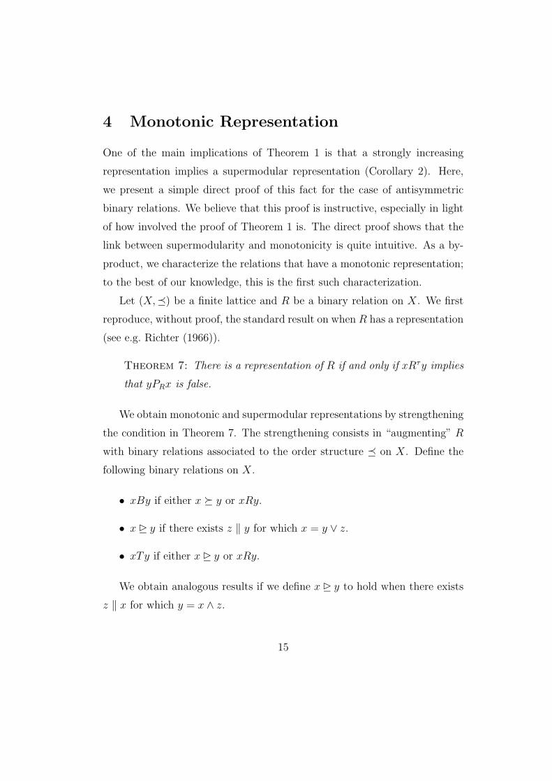
4 Monotonic Representation

One of the main implications of Theorem 1 is that a strongly increasing

representation implies a supermodular representation (Corollary 2). Here,

we present a simple direct proof of this fact for the case of antisymmetric

binary relations. We believe that this proof is instructive, especially in light

of how involved the proof of Theorem 1 is. The direct proof shows that the

link between supermodularity and monotonicity is quite intuitive. As a by-

product, we characterize the relations that have a monotonic representation;

to the best of our knowledge, this is the first such characterization.

Let (X,) be a finite lattice and R be a binary relation on X. We first

reproduce, without proof, the standard result on when R has a representation

(see e.g. Richter (1966)).

Theorem 7: There is a representation of R if and only if xRτy implies

that yPRx is false.

We obtain monotonic and supermodular representations by strengthening

the condition in Theorem 7. The strengthening consists in “augmenting” R

with binary relations associated to the order structure on X. Define the

following binary relations on X.

• xBy if either x y or xRy.

• x y if there exists z ‖ y for which x = y ∨ z.

• xTy if either x y or xRy.

We obtain analogous results if we define x y to hold when there exists

z ‖ x for which y = x ∧ z.

15

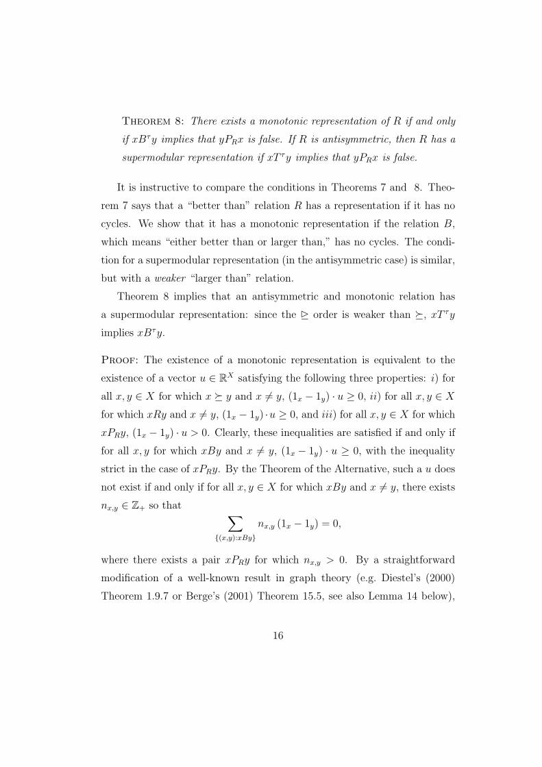
Theorem 8: There exists a monotonic representation of R if and only

if xBτy implies that yPRx is false. If R is antisymmetric, then R has a

supermodular representation if xT τy implies that yPRx is false.

It is instructive to compare the conditions in Theorems 7 and 8. Theo-

rem 7 says that a “better than” relation R has a representation if it has no

cycles. We show that it has a monotonic representation if the relation B,

which means “either better than or larger than,” has no cycles. The condi-

tion for a supermodular representation (in the antisymmetric case) is similar,

but with a weaker “larger than” relation.

Theorem 8 implies that an antisymmetric and monotonic relation has

a supermodular representation: since the order is weaker than , xT τy

implies xBτy.

Proof: The existence of a monotonic representation is equivalent to the

existence of a vector u ∈ RX satisfying the following three properties: i) for

all x, y ∈ X for which x y and x 6= y, (1x − 1y) · u ≥ 0, ii) for all x, y ∈ X

for which xRy and x 6= y, (1x − 1y) ·u ≥ 0, and iii) for all x, y ∈ X for which

xPRy, (1x − 1y) · u > 0. Clearly, these inequalities are satisfied if and only if

for all x, y for which xBy and x 6= y, (1x − 1y) · u ≥ 0, with the inequality

strict in the case of xPRy. By the Theorem of the Alternative, such a u does

not exist if and only if for all x, y ∈ X for which xBy and x 6= y, there exists

nx,y ∈ Z+ so that ∑(x,y):xBy

nx,y (1x − 1y) = 0,

where there exists a pair xPRy for which nx,y > 0. By a straightforward

modification of a well-known result in graph theory (e.g. Diestel’s (2000)

Theorem 1.9.7 or Berge’s (2001) Theorem 15.5, see also Lemma 14 below),

16

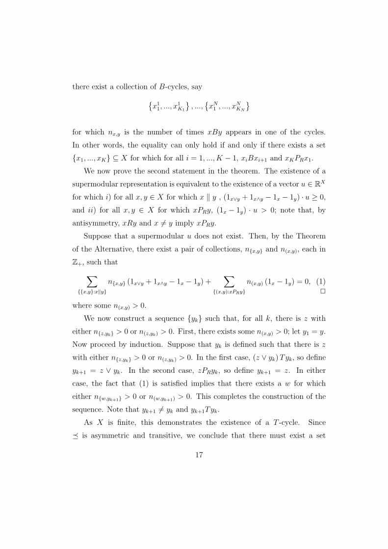
there exist a collection of B-cycles, sayx1

1, ..., x1K1

, ...,

xN

1 , ..., xNKN

for which nx,y is the number of times xBy appears in one of the cycles.

In other words, the equality can only hold if and only if there exists a set

x1, ..., xK ⊆ X for which for all i = 1, ..., K − 1, xiBxi+1 and xKPRx1.

We now prove the second statement in the theorem. The existence of a

supermodular representation is equivalent to the existence of a vector u ∈ RX

for which i) for all x, y ∈ X for which x ‖ y , (1x∨y + 1x∧y − 1x − 1y) · u ≥ 0,

and ii) for all x, y ∈ X for which xPRy, (1x − 1y) · u > 0; note that, by

antisymmetry, xRy and x 6= y imply xPRy.

Suppose that a supermodular u does not exist. Then, by the Theorem

of the Alternative, there exist a pair of collections, nx,y and n(x,y), each in

Z+, such that∑x,y:x‖y

nx,y (1x∨y + 1x∧y − 1x − 1y) +∑

(x,y):xPRy

n(x,y) (1x − 1y) = 0, (1)

2

where some n(x,y) > 0.

We now construct a sequence yk such that, for all k, there is z with

either nz,yk > 0 or n(z,yk) > 0. First, there exists some n(x,y) > 0; let y1 = y.

Now proceed by induction. Suppose that yk is defined such that there is z

with either nz,yk > 0 or n(z,yk) > 0. In the first case, (z ∨ yk) Tyk, so define

yk+1 = z ∨ yk. In the second case, zPRyk, so define yk+1 = z. In either

case, the fact that (1) is satisfied implies that there exists a w for which

either nw,yk+1 > 0 or n(w,yk+1) > 0. This completes the construction of the

sequence. Note that yk+1 6= yk and yk+1Tyk.

As X is finite, this demonstrates the existence of a T -cycle. Since

is asymmetric and transitive, we conclude that there must exist a set

17

x1, ..., xK ⊆ X for which for all i = 1, ..., K − 1, xiTxi+1, and xKPRx1.

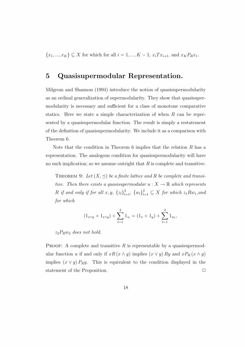
5 Quasisupermodular Representation.

Milgrom and Shannon (1994) introduce the notion of quasisupermodularity

as an ordinal generalization of supermodularity. They show that quasisuper-

modularity is necessary and sufficient for a class of monotone comparative

statics. Here we state a simple characterization of when R can be repre-

sented by a quasisupermodular function. The result is simply a restatement

of the definition of quasisupermodularity. We include it as a comparison with

Theorem 6.

Note that the condition in Theorem 6 implies that the relation R has a

representation. The analogous condition for quasisupermodularity will have

no such implication; so we assume outright that R is complete and transitive.

Theorem 9: Let (X,) be a finite lattice and R be complete and transi-

tive. Then there exists a quasisupermodular u : X → R which represents

R if and only if for all x, y, zl2l=1, wl2

l=1 ⊆ X for which z1Rw1,and

for which

(1x∨y + 1x∧y) +2∑

l=1

1zl= (1x + 1y) +

2∑l=1

1wl,

z2PRw2 does not hold.

Proof: A complete and transitive R is representable by a quasisupermod-

ular function u if and only if xR (x ∧ y) implies (x ∨ y) Ry and xPR (x ∧ y)

implies (x ∨ y) PRy. This is equivalent to the condition displayed in the

statement of the Proposition. 2

18

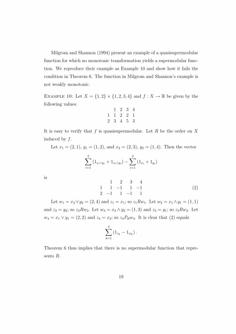
Milgrom and Shannon (1994) present an example of a quasisupermodular

function for which no monotonic transformation yields a supermodular func-

tion. We reproduce their example as Example 10 and show how it fails the

condition in Theorem 6. The function in Milgrom and Shannon’s example is

not weakly monotonic.

Example 10: Let X = 1, 2 × 1, 2, 3, 4 and f : X → R be given by the

following values:1 2 3 4

1 1 2 2 12 3 4 5 3

It is easy to verify that f is quasisupermodular. Let R be the order on X

induced by f .

Let x1 = (2, 1), y1 = (1, 2), and x2 = (2, 3), y2 = (1, 4). Then the vector

2∑i=1

(1xi∨yi+ 1xi∧yi

)−2∑

i=1

(1xi+ 1yi

)

is1 2 3 4

1 1 −1 1 −12 −1 1 −1 1

(2)

Let w1 = x2∨y2 = (2, 4) and z1 = x1; so z1Rw1. Let w2 = x1∧y1 = (1, 1)

and z2 = y2; so z2Rw2. Let w3 = x2 ∧ y2 = (1, 3) and z3 = y1; so z3Rw3. Let

w4 = x1 ∨ y1 = (2, 2) and z4 = x2; so z4PRw4. It is clear that (2) equals

4∑k=1

(1zk− 1wk

) .

Theorem 6 thus implies that there is no supermodular function that repre-

sents R.

19

6 Application 1: Afriat’s Model

Afriat (1967) studies how data on consumption choices at different prices can

refute assumptions on consumer preferences (see also Varian (1982)). Afriat

shows that the data can arise from a rational consumer if and only if one can

model the consumer with a monotone and concave utility function. Concavity

of utility is thus not refutable with data on consumption expenditures. In

a similar vein, we prove that supermodularity is not refutable with data on

consumption.2

The are long-standing doubts about the empirical content of supermodu-

larity in consumption theory. Allen (1934), Hicks and Allen (1934), Samuel-

son (1947), and Stigler (1950) believed that supermodularity has no empirical

implications for consumer behavior. Their doubts come from the realization

that supermodularity is not a cardinal property and that, at any point, there

is a representation of utility for which marginal utility is locally increasing

and one for which it is locally decreasing.

These doubts prove to be misleading. First, Chipman (1977), addressing

explicitly the critique of Allen, Hicks, Samuelson and Stigler, shows that a

consumer with a supermodular and strongly concave utility has a normal

demand. Chipman suggests that, as a result, supermodularity has testable

implications. Second, Milgrom and Shannon (1994) show that quasisuper-

modularity is an ordinal notion of complementarity and that it is implied by

supermodularity. So supermodularity has an ordinal implication which has

a natural interpretation as a complementarity property.

We address the testability of supermodularity using an explicit model of

2This section is better thanks to Ed Schlee’s and Chris Shannon’s suggestions. Edpointed us to the implications of the joint assumption of concavity and supermodularityand Chris suggested the proof using Chiappori and Rochet’s and Li Calzi’s results.

20

the data one might use to test it: Let X ⊆ Rn+ be a finite lattice. Let the pairs

(xk, Sk), k = 1, . . . , K, be such that Sk ⊆ X and xk ∈ Sk for all k. Interpret

each (xk, Sk) as one observation of the consumption bundle xk chosen by an

individual out of the budget set Sk. Arguably, this is the right model for the

question of whether supermodularity has empirical implications in consumer

theory. The model is Matzkin’s (1991) generalization of Afriat’s model.

We make three assumptions on the data:

1. For all k, xk ∈ ∂Sk; a “non-satiation” assumption.

2. If x ∈ Sk and y ≤ x then y ∈ Sk; if x is “affordable” in budget Sk, and

y is weakly less consumption of all goods, then y is also affordable.

3. If xk′ ∈ Sk and xk′ 6= xk, then xk /∈ Sk′ ; a version of the weak axiom of

revealed preference.

Consider the binary relation R on X defined by xRy if there is k such

that x = xk and y ∈ Sk. Note that R is the standard revealed-preference

relation. Note that xPRy if xRy and x 6= y.

Say that u : X → R rationalizes the data (xk, Sk)Kk=1 if it represents

R. Hence, a consumer with utility u would rationally choose xk out of Sk,

for each k. The function u is called a rationalization of the data. Under

Property 3, this notion of rationalization coincides with Afriat’s (1967).

Proposition 11: The data (xk, Sk)Kk=1 has a rationalization if and only

if it has a supermodular rationalization.

Proof: Let B be the binary relation defined as xBy if xRy or x ≥ y. It

is easily verified that xPBy if xPRy or x > y. We show below that R has a

representation if and only if B has a representation. The proposition then

21

follows from Corollary 2, because any representation of B must be strongly

monotone.

By Theorem 7, if B has a representation, then so does R. Suppose, by

means of contradiction, that B does not have a representation. We will show

that R does not have a representation.

If B does not have a representation, then there exist x, y ∈ X for which

xBτy and yPBx. Suppose that x ≥ y. Then yPBx implies that there exists

k for which y = xk. But y ∈ ∂Sk, so x ≥ y implies x = y, contradicting

the fact that yPBx. Therefore, x y. Hence, xBτy implies that there

exists x1, . . . xL ⊆ X for which xBx1B . . . BxLBy, where at least one B

corresponds to R and not ≥.

We claim that there exists x′ 6= y for which x ≥ x′ and x′Rτy. To

see this, note that for any collection of data z1, ..., zm ⊆ X for which

z1Rz2 ≥ z3 ≥ ... ≥ zm, it follows by the fact that z2 ≥ zm and Property 2 of

the data that z1Rzm. From this fact, we establish that there is x′ 6= y with

x ≥ x′ and x′Rτy.

As yPBx, either yPRx or y > x. If yPRx, then yPRx′ by x ≥ x′ and Prop-

erty 2 of the data. In this case, we may conclude that R has no representation

(Theorem 7). If instead y > x, then we have x′Rτy and y > x′. Then, x′Ry

contradicts Property 1 of the data, so there exists x′′ ∈ X, x′′ 6= x′ for which

x′Rτx′′Ry. Now, y ≥ x′ and Property2 of the data imply that x′′Rx′. In fact,

by Property 3 and x′′ 6= x′, x′′PRx′. So R does not have a representation. 2

Our model is related to Afriat’s in the following way. Afriat’s data consists

of pairs (xk, pk), k = 1, . . . , K, such that xk ∈ X ⊆ Rn+ and pk ∈ Rn

++, for

all k. Each pair is an observed consumption choice xk at prices pk. Afriat’s

22

data are obtained from ours by setting

Sk =x : pk · x ≤ pk · xk

.

Note that the weak axiom, Property 3 of the data, is implicit in Afriat’s

results. If we do not assume Property 3 we would need to distinguish be-

tween representability of R and rationalization; the result in Proposition 11

continues to hold.

Our model allows us to more generally accommodate non-linear bud-

gets sets; Matzkin (1991) introduced this model as a way of discussing the

issues raised by Afriat’s results in situations where consumers have monop-

sony power, or where the consumer is a social planner facing an economy’s

production possibility set.

With Afriat’s data, there is a very direct proof of our result: Afriat’s

theorem implies that, if the data are rationalizable, R has a strongly mono-

tonic representation (the utility he constructs is the lower envelope of a finite

number of strongly monotonic linear functions). Then, by Corollary 2, R has

a supermodular representation.

Two remarks are in order. First, under an additional restriction on

Afriat’s data, rationalizability implies that there is a smooth, strongly mono-

tonic rationalization (Chiappori and Rochet, 1987). Corollary 20 in Li Calzi

(1990) then implies the existence of a supermodular rationalization. So one

can use existing results to prove a version of Proposition 11 for the Afriat

data under Chiappori and Rochet’s assumptions.

The second remark refers to concave rationalizations. Afriat shows that

having a rationalization is equivalent to having a rationalization by a concave

function and Proposition 11 says that it is equivalent to a rationalization

by a supermodular function. One might conjecture that any rationalizable

23

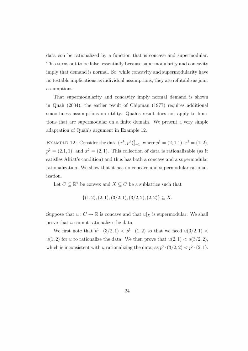
data con be rationalized by a function that is concave and supermodular.

This turns out to be false, essentially because supermodularity and concavity

imply that demand is normal. So, while concavity and supermodularity have

no testable implications as individual assumptions, they are refutable as joint

assumptions.

That supermodularity and concavity imply normal demand is shown

in Quah (2004); the earlier result of Chipman (1977) requires additional

smoothness assumptions on utility. Quah’s result does not apply to func-

tions that are supermodular on a finite domain. We present a very simple

adaptation of Quah’s argument in Example 12.

Example 12: Consider the data (xk, pk)2k=1, where p1 = (2, 1.1), x1 = (1, 2),

p2 = (2.1, 1), and x2 = (2, 1). This collection of data is rationalizable (as it

satisfies Afriat’s condition) and thus has both a concave and a supermodular

rationalization. We show that it has no concave and supermodular rational-

ization.

Let C ⊆ R2 be convex and X ⊆ C be a sublattice such that

(1, 2), (2, 1), (3/2, 1), (3/2, 2), (2, 2) ⊆ X.

Suppose that u : C → R is concave and that u|X is supermodular. We shall

prove that u cannot rationalize the data.

We first note that p1 · (3/2, 1) < p1 · (1, 2) so that we need u(3/2, 1) <

u(1, 2) for u to rationalize the data. We then prove that u(2, 1) < u(3/2, 2),

which is inconsistent with u rationalizing the data, as p2 ·(3/2, 2) < p2 ·(2, 1).

24

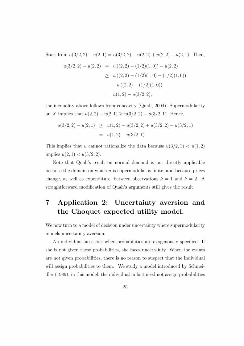
Start from u(3/2, 2)− u(2, 1) = u(3/2, 2)− u(2, 2) + u(2, 2)− u(2, 1). Then,

u(3/2, 2)− u(2, 2) = u ((2, 2)− (1/2)(1, 0))− u(2, 2)

≥ u ((2, 2)− (1/2)(1, 0)− (1/2)(1, 0))

−u ((2, 2)− (1/2)(1, 0))

= u(1, 2)− u(3/2, 2);

the inequality above follows from concavity (Quah, 2004). Supermodularity

on X implies that u(2, 2)− u(2, 1) ≥ u(3/2, 2)− u(3/2, 1). Hence,

u(3/2, 2)− u(2, 1) ≥ u(1, 2)− u(3/2, 2) + u(3/2, 2)− u(3/2, 1)

= u(1, 2)− u(3/2, 1).

This implies that u cannot rationalize the data because u(3/2, 1) < u(1, 2)

implies u(2, 1) < u(3/2, 2).

Note that Quah’s result on normal demand is not directly applicable

because the domain on which u is supermodular is finite, and because prices

change, as well as expenditure, between observations k = 1 and k = 2. A

straightforward modification of Quah’s arguments still gives the result.

7 Application 2: Uncertainty aversion and

the Choquet expected utility model.

We now turn to a model of decision under uncertainty where supermodularity

models uncertainty aversion.

An individual faces risk when probabilities are exogenously specified. If

she is not given these probabilities, she faces uncertainty. When the events

are not given probabilities, there is no reason to suspect that the individual

will assign probabilities to them. We study a model introduced by Schmei-

dler (1989); in this model, the individual in fact need not assign probabilities

25

to events, but assigns some measure of likelihood to them. This measure is

called a capacity. Supermodularity of the capacity in this model is inter-

preted as uncertainty aversion.

Our results imply that Schmeidler’s notion of uncertainty aversion places

few restrictions on the individual’s preferences over bets. As a consequence, if

one can elicit her likelihood ranking of events, it is very difficult to refute that

she is uncertainty averse (for example if larger events are always perceived

as strictly more likely, uncertainty aversion cannot be refuted). We briefly

describe Schmeidler’s model and explain the implications of our results.

Let Ω be a finite set of possible states of the world and let Y be a set of

possible outcomes. The set of (Anscombe and Aumann, 1963) acts is the

set of functions f : Ω → ∆ (Y ). Denote the set of acts by F . A capacity is

a function ν : 2Ω → R for which ν (∅) = 0, ν (Ω) = 1, and A ⊆ B implies

ν (A) ≤ ν (B). A capacity is supermodular if it is supermodular when 2Ω

is endowed with the set-inclusion order.

A binary relation R over F conforms to the Choquet expected utility

model if there exists some u : ∆ (Y ) → R conforming to the von Neumann-

Morgenstern axioms and a capacity ν on Ω for which the function U : F → Rrepresents R, where

U (f) ≡∫

Ω

u (f (ω)) dν (ω) ; 3 (2)

Schmeidler (1989) axiomatizes those R conforming to the Choquet expected

utility model. A binary relation R which conforms to the Choquet expected

3The Choquet integral with respect to ν is defined as:∫Ω

g (ω) dν (ω)

=∫ +∞

0

ν (ω : g (ω) > t) dt +∫ 0

−∞[ν (ω : g (ω) > t)− 1] dt

26

utility model exhibits Schmeidler uncertainty aversion if and only if ν

is supermodular.

For a given binary relation R over F conforming to the Choquet expected

utility model, define the likelihood relation R∗ over 2Ω by ER∗F if there exist

x, y ∈ X for which xPRy4 and[x if ω ∈ Ey if ω /∈ E

]R

[x if ω ∈ Fy if ω /∈ F

].

The likelihood relation reflects a “willingness to bet.” If ER∗F , then the

individual prefers to place stakes on E as opposed to F . For the Choquet

expected utility model, this relation is complete. We will write the asym-

metric part of R∗ by P ∗ and the symmetric part by I∗. The following is an

immediate corollary to Theorem 1, using the fact that all likelihood relations

are weakly increasing.

Proposition 13: Suppose that R conforms to the Choquet expected

utility model. Then the likelihood relation R∗ is incompatible with Schmei-

dler uncertainty aversion if and only if there exist events A, B, C ⊆ Ω for

which A ⊆ B and B ∩ C = ∅ for which (A ∪ C) P ∗A and (B ∪ C) I∗B.

First, note that Schmeidler uncertainty aversion can never be refuted

when the likelihood relation R∗ is strictly monotonic. This observation fol-

lows from Proposition 13 for the same reason that Corollary 2 follows from

Theorem 1. Hence, if an individual always strictly prefers to bet on larger

events, one cannot refute that she is uncertainty averse.

Second, even in the case when R∗ is not strictly monotonic, uncertainty

aversion is difficult to refute. Using the notation in Proposition 13, it requires

4Here we are abusing notation by identifying a constant act with the value that constantact takes.

27

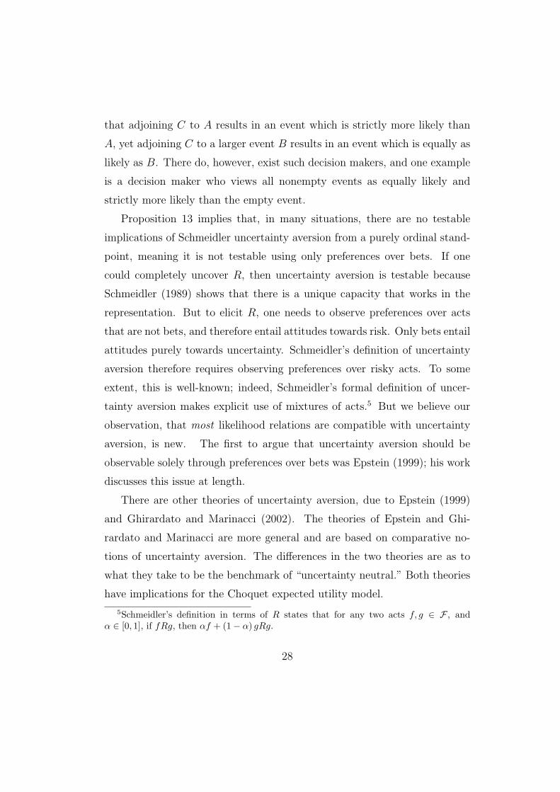
that adjoining C to A results in an event which is strictly more likely than

A, yet adjoining C to a larger event B results in an event which is equally as

likely as B. There do, however, exist such decision makers, and one example

is a decision maker who views all nonempty events as equally likely and

strictly more likely than the empty event.

Proposition 13 implies that, in many situations, there are no testable

implications of Schmeidler uncertainty aversion from a purely ordinal stand-

point, meaning it is not testable using only preferences over bets. If one

could completely uncover R, then uncertainty aversion is testable because

Schmeidler (1989) shows that there is a unique capacity that works in the

representation. But to elicit R, one needs to observe preferences over acts

that are not bets, and therefore entail attitudes towards risk. Only bets entail

attitudes purely towards uncertainty. Schmeidler’s definition of uncertainty

aversion therefore requires observing preferences over risky acts. To some

extent, this is well-known; indeed, Schmeidler’s formal definition of uncer-

tainty aversion makes explicit use of mixtures of acts.5 But we believe our

observation, that most likelihood relations are compatible with uncertainty

aversion, is new. The first to argue that uncertainty aversion should be

observable solely through preferences over bets was Epstein (1999); his work

discusses this issue at length.

There are other theories of uncertainty aversion, due to Epstein (1999)

and Ghirardato and Marinacci (2002). The theories of Epstein and Ghi-

rardato and Marinacci are more general and are based on comparative no-

tions of uncertainty aversion. The differences in the two theories are as to

what they take to be the benchmark of “uncertainty neutral.” Both theories

have implications for the Choquet expected utility model.

5Schmeidler’s definition in terms of R states that for any two acts f, g ∈ F , andα ∈ [0, 1], if fRg, then αf + (1− α) gRg.

28

8 Conclusion

We provide a characterization of the preferences which have a supermodular

representation. For weakly monotonic preferences, supermodularity is equiv-

alent to quasisupermodularity, Milgrom and Shannon’s (1994) ordinal notion

of complementarities.

Our results confirm the intuition of Allen (1934), Hicks and Allen (1934),

Samuelson (1947), and Stigler (1950) that supermodularity is void of em-

pirical meaning in ordinal economic environments. We have established this

in two important economic models—a generalized version of Afriat’s model

and the Choquet expected utility model. We have shown that any strictly

increasing function on a finite lattice can be ordinally transformed into a

supermodular function. One issue that we have not dealt with is the the-

ory of supermodular functions on infinite lattices. Obviously, not all strictly

increasing binary relations on infinite lattices are representable by supermod-

ular functions–just consider the standard lexicographic order on R2, which is

not even representable. However, our results are meant to apply to testable

environments, or environments in which a finite set of data can be observed.

Thus, from an empirical perspective, we do not believe the restriction to

finite lattices is problematic.

9 Proof of Theorem 1

In this section, we provide a proof of Theorem 1. We emphasize that the

proof can be adapted to show the equivalence of quasisupermodularity and

supermodularity for weakly decreasing binary relations.

In one direction, the theorem is trivial: if R has a weakly increasing super-

modular representation, then this representation is also quasisupermodular.

29

In the rest of this section we show that, if R is weakly increasing and qua-

sisupermodular, then it has a supermodular representation; the property of

being weakly increasing is ordinal, so the resulting supermodular represen-

tation will be weakly increasing.

Let R be monotonic, quasisupermodular, and representable. We need

some preliminary definitions.

A multigraph is a pair G = (X, E), where X is a finite set and E is a

matrix with |X| columns; each column is identified with an element of X,

and each row can be written as 1x − 1y for two distinct x, y ∈ X. Abusing

notation, we identify rows 1x − 1y with the pair (x, y) and refer to (x, y) as

an edge. Note that there may be more than one edge (x, y), as there may

be more than one copy of the row 1x − 1y in E (herein lies the notational

abuse).

A cycle for a multigraph (X, E) is a sequence zini=1 with (zi+1, zi) ∈ E

(modulo n). We say that zi+1 follows zi in the cycle.

Say that (X, E) can be partitioned into cycleszk

i

nk

i=1, k = 1, . . . , K

if,

• for each k,zk

i

nk

i=1is a cycle,

• X = ∪zk

i : i = 1, . . . , nk, k = 1, . . . , K,

• for each two distinct x, y ∈ X, the number of rows 1x − 1y equals the

number of times x follows y in one of the cycles.

We state the following lemma without proof. The lemma follows from a

straightforward modification of, for example, Diestel’s (2000) Theorem 1.9.7

or Berge’s (2001) Theorem 15.5.

Lemma 14: If the sum of the rows of E equals the null vector in RX ,

then (X, E) has a partition into cycles.

30

We define a canonical multigraph G as a multigraph, the edges of

which can be partitioned into four edge sets: EGR , EG

P , EG∨ , and EG

∧ , which

satisfy the following seven properties:

i) If (x, y) ∈ EGR , then (x, y) ∈ R \ P

ii) If (x, y) ∈ EGP , then (x, y) ∈ P

iii) If (x, y) ∈ EG∧ , then there exists z ∈ X for which y ‖ z and x = z ∧ y

iv) If (x, y) ∈ EG∨ , then there exists z ∈ X for which y ‖ z and x = z ∨ y,

v) G can be partitioned into cycles

vi) EGP 6= ∅

vii) If (y ∧ x, x) ∈ EG∧ and xP (y ∧ x), then (x ∨ y, y) ∈ EG

∨ .

The proof proceeds by contradiction. We first outline the steps involved.

First, we show that if there does not exist a supermodular representation,

then there exists a canonical multigraph. We then show that, for any canon-

ical multigraph, there must exist (y ∧ x, x) ∈ EG∧ for which xP (y ∧ x). We

also show that if G is a canonical multigraph, there exists another canonical

multigraph G′ for which there are strictly less elements (y ∧ x, x) ∈ EG∧ for

which xP (y ∧ x). These latter two statements taken together are directly

contradictory.

The new canonical multigraph will be constructed by adding a collection

of edges to EGR which themselves can be partitioned into cycles. These ad-

ditional edges are used to construct a large cycle which includes elements

(y ∧ x, x) ∈ EG∧ for which xP (y ∧ x). The large cycle will never contain

31

an element (x ∨ y, y) ∈ EG∨ for which (x ∨ y) Py without containing a cor-

responding element (x ∧ y, x) ∈ EG∧ . By removing this large cycle, we will

have a new multigraph satisfying all of the appropriate conditions.

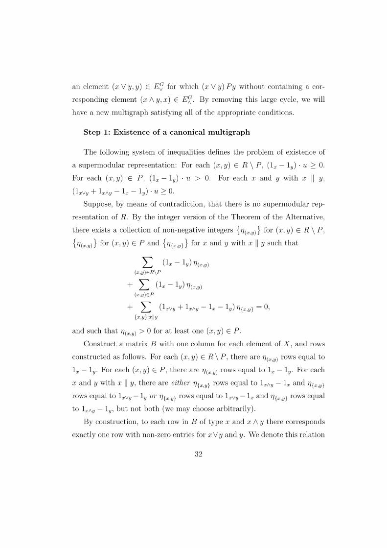
Step 1: Existence of a canonical multigraph

The following system of inequalities defines the problem of existence of

a supermodular representation: For each (x, y) ∈ R \ P , (1x − 1y) · u ≥ 0.

For each (x, y) ∈ P , (1x − 1y) · u > 0. For each x and y with x ‖ y,

(1x∨y + 1x∧y − 1x − 1y) · u ≥ 0.

Suppose, by means of contradiction, that there is no supermodular rep-

resentation of R. By the integer version of the Theorem of the Alternative,

there exists a collection of non-negative integersη(x,y)

for (x, y) ∈ R \ P ,

η(x,y)

for (x, y) ∈ P and

ηx,y

for x and y with x ‖ y such that∑

(x,y)∈R\P

(1x − 1y) η(x,y)

+∑

(x,y)∈P

(1x − 1y) η(x,y)

+∑

x,y:x‖y

(1x∨y + 1x∧y − 1x − 1y) ηx,y = 0,

and such that η(x,y) > 0 for at least one (x, y) ∈ P .

Construct a matrix B with one column for each element of X, and rows

constructed as follows. For each (x, y) ∈ R \P , there are η(x,y) rows equal to

1x − 1y. For each (x, y) ∈ P , there are η(x,y) rows equal to 1x − 1y. For each

x and y with x ‖ y, there are either ηx,y rows equal to 1x∧y − 1x and ηx,y

rows equal to 1x∨y−1y or ηx,y rows equal to 1x∨y−1x and ηx,y rows equal

to 1x∧y − 1y, but not both (we may choose arbitrarily).

By construction, to each row in B of type x and x ∧ y there corresponds

exactly one row with non-zero entries for x∨y and y. We denote this relation

32

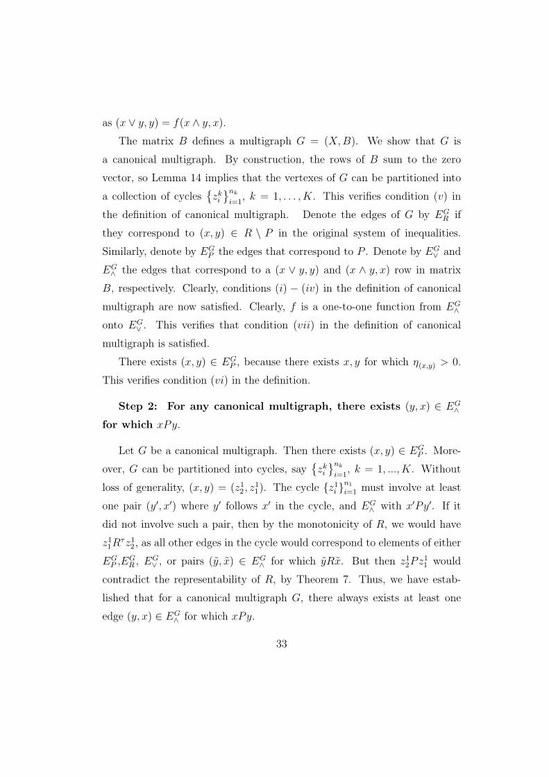
as (x ∨ y, y) = f(x ∧ y, x).

The matrix B defines a multigraph G = (X, B). We show that G is

a canonical multigraph. By construction, the rows of B sum to the zero

vector, so Lemma 14 implies that the vertexes of G can be partitioned into

a collection of cycleszk

i

nk

i=1, k = 1, . . . , K. This verifies condition (v) in

the definition of canonical multigraph. Denote the edges of G by EGR if

they correspond to (x, y) ∈ R \ P in the original system of inequalities.

Similarly, denote by EGP the edges that correspond to P . Denote by EG

∨ and

EG∧ the edges that correspond to a (x ∨ y, y) and (x ∧ y, x) row in matrix

B, respectively. Clearly, conditions (i) − (iv) in the definition of canonical

multigraph are now satisfied. Clearly, f is a one-to-one function from EG∧

onto EG∨ . This verifies that condition (vii) in the definition of canonical

multigraph is satisfied.

There exists (x, y) ∈ EGP , because there exists x, y for which η(x,y) > 0.

This verifies condition (vi) in the definition.

Step 2: For any canonical multigraph, there exists (y, x) ∈ EG∧

for which xPy.

Let G be a canonical multigraph. Then there exists (x, y) ∈ EGP . More-

over, G can be partitioned into cycles, sayzk

i

nk

i=1, k = 1, ..., K. Without

loss of generality, (x, y) = (z12 , z

11). The cycle z1

i n1

i=1 must involve at least

one pair (y′, x′) where y′ follows x′ in the cycle, and EG∧ with x′Py′. If it

did not involve such a pair, then by the monotonicity of R, we would have

z11R

τz12 , as all other edges in the cycle would correspond to elements of either

EGP ,EG

R , EG∨ , or pairs (y, x) ∈ EG

∧ for which yRx. But then z12Pz1

1 would

contradict the representability of R, by Theorem 7. Thus, we have estab-

lished that for a canonical multigraph G, there always exists at least one

edge (y, x) ∈ EG∧ for which xPy.

33

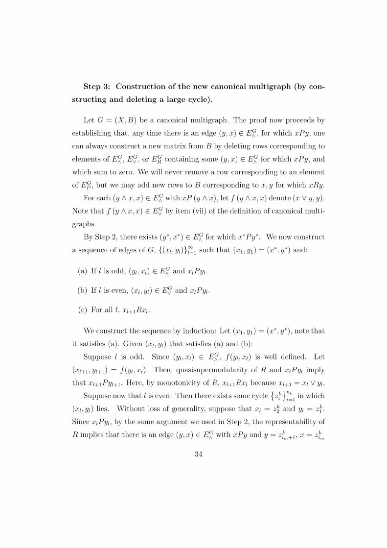
Step 3: Construction of the new canonical multigraph (by con-

structing and deleting a large cycle).

Let G = (X, B) be a canonical multigraph. The proof now proceeds by

establishing that, any time there is an edge (y, x) ∈ EG∧ , for which xPy, one

can always construct a new matrix from B by deleting rows corresponding to

elements of EG∧ , EG

∨ , or EGR containing some (y, x) ∈ EG

∧ for which xPy, and

which sum to zero. We will never remove a row corresponding to an element

of EGP , but we may add new rows to B corresponding to x, y for which xRy.

For each (y ∧ x, x) ∈ EG∧ with xP (y ∧ x), let f (y ∧ x, x) denote (x ∨ y, y).

Note that f (y ∧ x, x) ∈ EG∨ by item (vii) of the definition of canonical multi-

graphs.

By Step 2, there exists (y∗, x∗) ∈ EG∧ for which x∗Py∗. We now construct

a sequence of edges of G, (xl, yl)∞l=1 such that (x1, y1) = (x∗, y∗) and:

(a) If l is odd, (yl, xl) ∈ EG∧ and xlPyl.

(b) If l is even, (xl, yl) ∈ EG∨ and xlPyl.

(c) For all l, xl+1Rxl.

We construct the sequence by induction: Let (x1, y1) = (x∗, y∗), note that

it satisfies (a). Given (xl, yl) that satisfies (a) and (b):

Suppose l is odd. Since (yl, xl) ∈ EG∧ , f(yl, xl) is well defined. Let

(xl+1, yl+1) = f(yl, xl). Then, quasisupermodularity of R and xlPyl imply

that xl+1Pyl+1. Here, by monotonicity of R, xl+1Rxl because xl+1 = xl ∨ yl.

Suppose now that l is even. Then there exists some cyclezk

i

nk

i=1in which

(xl, yl) lies. Without loss of generality, suppose that xl = zk2 and yl = zk

1 .

Since xlPyl, by the same argument we used in Step 2, the representability of

R implies that there is an edge (y, x) ∈ EG∧ with xPy and y = zk

im+1, x = zkim

34

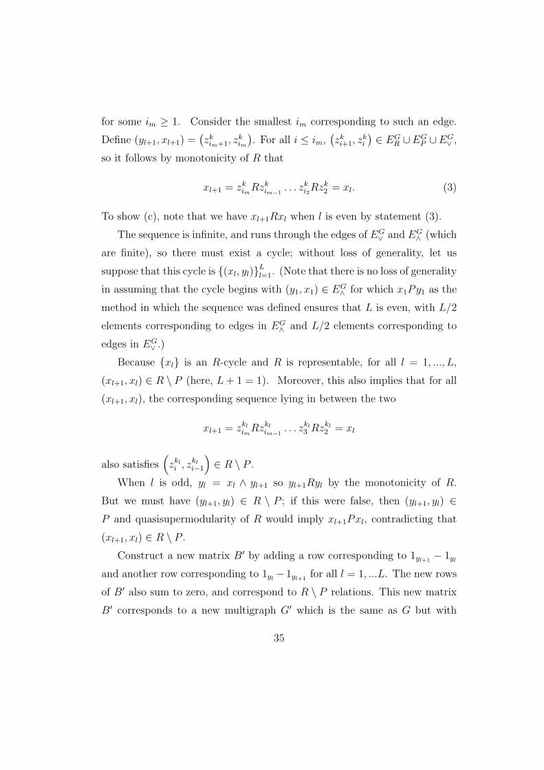
for some im ≥ 1. Consider the smallest im corresponding to such an edge.

Define (yl+1, xl+1) =(zk

im+1, zkim

). For all i ≤ im,

(zk

i+1, zki

)∈ EG

R ∪EGP ∪EG

∨ ,

so it follows by monotonicity of R that

xl+1 = zkimRzk

im−1. . . zk

i2Rzk

2 = xl. (3)

To show (c), note that we have xl+1Rxl when l is even by statement (3).

The sequence is infinite, and runs through the edges of EG∨ and EG

∧ (which

are finite), so there must exist a cycle; without loss of generality, let us

suppose that this cycle is (xl, yl)Ll=1. (Note that there is no loss of generality

in assuming that the cycle begins with (y1, x1) ∈ EG∧ for which x1Py1 as the

method in which the sequence was defined ensures that L is even, with L/2

elements corresponding to edges in EG∧ and L/2 elements corresponding to

edges in EG∨ .)

Because xl is an R-cycle and R is representable, for all l = 1, ..., L,

(xl+1, xl) ∈ R \ P (here, L + 1 = 1). Moreover, this also implies that for all

(xl+1, xl), the corresponding sequence lying in between the two

xl+1 = zklim

Rzklim−1

. . . zkl3 Rzkl

2 = xl

also satisfies(zkl

i , zkli−1

)∈ R \ P .

When l is odd, yl = xl ∧ yl+1 so yl+1Ryl by the monotonicity of R.

But we must have (yl+1, yl) ∈ R \ P ; if this were false, then (yl+1, yl) ∈P and quasisupermodularity of R would imply xl+1Pxl, contradicting that

(xl+1, xl) ∈ R \ P .

Construct a new matrix B′ by adding a row corresponding to 1yl+1− 1yl

and another row corresponding to 1yl− 1yl+1

for all l = 1, ...L. The new rows

of B′ also sum to zero, and correspond to R \ P relations. This new matrix

B′ corresponds to a new multigraph G′ which is the same as G but with

35

additional edges, (yl+1, yl), and (yl, yl+1), each lying in EG′R . The rows of B′

also clearly sum to zero, as the rows we have added sum to zero.

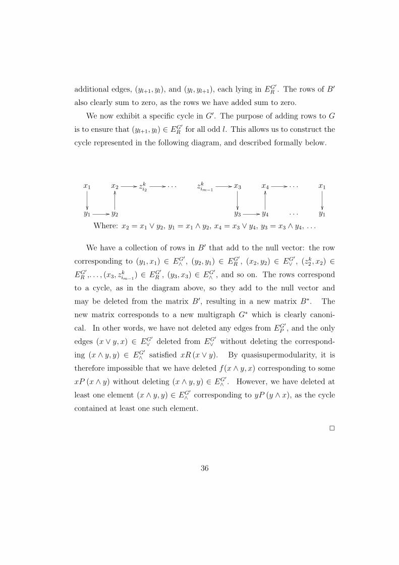
We now exhibit a specific cycle in G′. The purpose of adding rows to G

is to ensure that (yl+1, yl) ∈ EG′R for all odd l. This allows us to construct the

cycle represented in the following diagram, and described formally below.

x1

x2 // zki2

// . . . zkim−1

// x3

x4 // . . . x1

y1 // y2

OO

y3 // y4

OO

. . . y1

Where: x2 = x1 ∨ y2, y1 = x1 ∧ y2, x4 = x3 ∨ y4, y3 = x3 ∧ y4, . . .

We have a collection of rows in B′ that add to the null vector: the row

corresponding to (y1, x1) ∈ EG′∧ , (y2, y1) ∈ EG′

R , (x2, y2) ∈ EG′∨ , (zk

2 , x2) ∈EG′

R ,. . . , (x3, zkim−1

) ∈ EG′R , (y3, x3) ∈ EG′

∧ , and so on. The rows correspond

to a cycle, as in the diagram above, so they add to the null vector and

may be deleted from the matrix B′, resulting in a new matrix B∗. The

new matrix corresponds to a new multigraph G∗ which is clearly canoni-

cal. In other words, we have not deleted any edges from EG′P , and the only

edges (x ∨ y, x) ∈ EG′∨ deleted from EG′

∨ without deleting the correspond-

ing (x ∧ y, y) ∈ EG′∧ satisfied xR (x ∨ y). By quasisupermodularity, it is

therefore impossible that we have deleted f(x ∧ y, x) corresponding to some

xP (x ∧ y) without deleting (x ∧ y, y) ∈ EG′∧ . However, we have deleted at

least one element (x ∧ y, y) ∈ EG′∧ corresponding to yP (y ∧ x), as the cycle

contained at least one such element.

2

36

References

Afriat, S. N. (1967): “The Construction of Utility Functions from Expen-

diture Data,” International Economic Review, 8(1), 67–77.

Allen, R. G. D. (1934): “A Comparison Between Different Definitions of

Complementary and Competitive Goods,” Econometrica, 2(2), 168–175.

Anscombe, F., and R. Aumann (1963): “A Definition of Subjective Prob-

ability,” Annals of Mathematical Statistics, 34, 199–205.

Athey, S., P. Milgrom, and J. Roberts (1998): “Robust Comparative

Statics,” Mimeo, Stanford University.

Aumann, R. J. (1964): “Subjective Programming,” in Human Judgments

and Optimality, ed. by M. Shelley, and G. L. Bryan. Wiley. New York.

Becker, G. S. (1973): “A Theory of Marriage: Part I,” Journal of Political

Economy, 81(4), 813–846.

Berge, C. (2001): Theory of Graphs. Dover.

Chiappori, P.-A., and J.-C. Rochet (1987): “Revealed Preferences and

Differentiable Demand,” Econometrica, 55(3), 687–691.

Chipman, J. S. (1977): “An empirical implication of Auspitz-Lieben-

Edgeworth-Pareto complementarity,” Journal of Economic Theory, 14(1),

228–231.

Chung-Piaw, T., and R. Vohra (2003): “Afriat’s Theorem and Negative

Cycles,” Mimeo, Northwestern University.

Diestel, R. (2000): Graph Theory. Springer.

37

Epstein, L. G. (1999): “A Definition of Uncertainty Aversion,” Review of

Economic Studies, 66(3), 579–608.

Fishburn, P. C. (1970): Utility Theory for Decision Making. Wiley, New

York.

Fostel, A., H. Scarf, and M. Todd (2004): “Two New Proofs of Afriat‘s

Theorem,” Economic Theory, 24(1), 211–219.

Ghirardato, P., and M. Marinacci (2002): “Ambiguity Made Precise:

A Comparative Foundation,” Journal of Economic Theory, 102(2), 251–

289.

Hicks, J. R., and R. G. D. Allen (1934): “A Reconsideration of the

Theory of Value. Part I,” Economica, 1(1), 52–76.

Kannai, Y. (2005): “Remarks concerning concave utility functions on finite

sets,” Economic Theory,, 26(2), 333–344.

Kreps, D. M. (1979): “A Representation Theorem for “Preference for Flex-

ibility”,” Econometrica, 47(3), 565–578.

Li Calzi, M. (1990): “Generalized Symmetric Supermodular Functions,”

Mimeo, Stanford University.

Matzkin, R. L. (1991): “Axioms of Revealed Preference for Nonlinear

Choice Sets,” Econometrica, 59(6), 1779–1786.

Milgrom, P., and J. Roberts (1990): “Rationalizability, Learning and

Equilibrium in Games with Strategic Complementarities,” Econometrica,

58(6), 1255–1277.

38

Milgrom, P., and C. Shannon (1994): “Monotone Comparative Statics,”

Econometrica, 62(1), 157–180.

Nehring, K. (1999): “Preference for Flexibility in a Savage Framework,”

Econometrica, 67(1), 101–119.

Quah, J. K.-H. (2004): “The Comparative Statics of Constrained Opti-

mization Problems,” Mimeo, Oxford University.

Richter, M. K. (1966): “Revealed Preference Theory,” Econometrica,

34(3), 635–645.

Richter, M. K., and K.-C. Wong (2004): “Concave utility on finite

sets,” Journal of Economic Theory, 115(2), 341–357.

Samuelson, P. A. (1947): Foundations of Economic Analysis. Harvard

University Press.

(1974): “Complementarity: An Essay on The 40th Anniversary

of the Hicks-Allen Revolution in Demand Theory,” Journal of Economic

Literature, 12(4), 1255–1289.

Schmeidler, D. (1989): “Subjective probability and expected utility with-

out additivity,” Econometrica, 57(3), 571–587.

Shapley, L. S. (1971): “Cores of Convex Games,” International Journal

of Game Theory, 1(1), 11–26.

Stigler, G. J. (1950): “The Development of Utility Theory, II,” Journal

of Political Economy, 58(5), 373–396.

Topkis, D. M. (1978): “Minimizing a Submodular Function on a Lattice,”

Operations Research, 26(2), 305–321.

39

Topkis, D. M. (1979): “Equilibrium Points in Nonzero-Sum n-Person Sub-

modular Games,” SIAM Journal of Control and Optimization, 17(6), 773–

787.

(1998): Supermodularity and Complementarity. Princeton Univer-

sity Press, Princeton, New Jersey.

Varian, H. R. (1982): “The Nonparametric Approach to Demand Analy-

sis,” Econometrica, 50(4), 945–974.

Vives, X. (1990): “Nash Equilibrium with Strategic Complementarities,”

Journal of Mathematical Economics, 19(3), 305–321.

(1999): Oligopoly Pricing. MIT Press, Cambridge, Massachusetts.

(2005): “Complementarities and Games: New Developments,”

Journal of Economic Literature, 43(2), 437–479.

40