Supplementary Materials: Materials and Methods

Figures S1-S7

Tables S1-S12

Supplementary Materials: Supplementary Methods ABSOLUTE and Multiplicity

We used the ABSOLUTE method to analyze mutant allele fractions, taking into account local SCNAs and tumor purity to estimate the fraction of cancer cells containing the mutant allele, as well as the average number of alternate alleles per tumor cell (multiplicity). In addition, ABSOLUTE classified mutations as homozygous in cases with complete loss of the reference allele in the cancer cell population.

Multiplicity is a measure of the average number of alternate alleles per tumor cell for each site of somatic variation, and is estimated from the mutation AF, the local somatic copy number, and the tumor purity and ploidy (1). A multiplicity at the level of unity or above represents a clonal mutation while values less than 1 indicate that the mutation is subclonal. Each mutation was classified as clonal or sub-clonal according to the probability that the observed multiplicity was consistent with or exceeded unit multiplicity.

Whole Exome Capture Library Construction Library construction followed the procedure previously detailed in previous publications

(2-5). Exome targets were generated based on CCDS + RefSeq genes (http://www.ncbi.nlm.nih.gov/projects/CCDS/ and http://www.ncbi.nlm.nih.gov/RefSeq/), representing 188,260 exons from ~18,560 genes (93% of known, non-repetitive protein coding genes) and spanning ~1% of the genome (32.7 Mb). Genomic DNA from primary tumor and patient-matched blood normal was sheared, ligated to Illumina sequencing adapters, and selected for lengths between 75-300 bp. This “pond” of DNA was hybridized with an excess of biotinylated RNA “baits” in solution. The “catch” was pulled down by magnetic beads coated with streptavidin and eluted as described previously (6,7). Sequencing libraries were quantified using a SYBR Green qPCR protocol with specific probes complementary to adapter sequence. Based on the qPCR quantification, libraries were normalized to 2 nM and then denatured using 0.1 N NaOH. Cluster amplification of denatured templates was performed according to manufacturer’s protocol (Illumina) using V3 Chemistry and V3 Flowcells. SYBR Green dye was added to all flowcell lanes to provide a quality control checkpoint after cluster amplification and to ensure optimal cluster densities on the flowcells. Barcoded exon capture libraries were then pooled into batches of 96 samples and sequenced on Illumina HiSeq instrument (76 bp paired-end reads) (6). The 8 bp barcode index was read by the instrument at the beginning of read 2 and used to distribute sequencing reads to sample in the downstream data aggregation. Standard quality control metrics--including error rates, % passing filter reads, and total Gb produced—

were used to characterize process performance prior to downstream analysis. The median coverage achieved across all exome samples in the data set was 90X for tumor and 86.5X for normal samples. Sequence data processing

Massively parallel sequencing data were processed using two consecutive pipelines:

(1) The sequencing data processing pipeline, called “Picard”, developed by the Sequencing Platform at the Broad Institute, starts with the reads and qualities produced by the Illumina software for all lanes and libraries generated for a single sample (either tumor or normal) and produces, at the end of the pipeline, a single BAM file (http://samtools.sourceforge.net/SAM1.pdf) for each tumor and matched normal sample. The final BAM file stores all reads with re-calibrated qualities together with their alignments to the genome (only for reads that were successfully aligned).

(2) The Broad Cancer Genome Analysis pipeline, also known as “Firehose”, starts with the BAM files for the tumor and matched normal samples and performs various analyses, including quality control, local realignment, mutation calling, small insertion and deletion identification, rearrangement detection, coverage calculations and others (see details below).

Several of the tools used in these pipelines were developed jointly by the Broad Institute Sequencing Platform, Medical and Population Genetics Program and the Cancer Program. Additional details regarding parts of the pipeline focused on germline events (typically employed for medical and population genetics studies) are described elsewhere (8).

The sequencing data-processing pipeline (“Picard pipeline”) We generated a BAM file for each sample using the sequencing data processing pipeline

known as “Picard” (http://picard.sourceforge.net/). Picard consists of four steps, described in detail in Chapman, M.A. et al. (3), but with the following modifications in the “Alignment to the genome” step: Alignment was performed using BWA (http://bio-bwa.sourceforge.net/) to the NCBI Human Reference Genome GRCh37 (9).

The reads in the BAM file were sorted according to their chromosomal position. Unaligned reads were also stored in the BAM file such that all reads that passed the Illumina purity filter were kept in the BAM. Duplicate reads were marked such that only unique sequenced DNA fragments were used in subsequent analysis.

Local realignment. Sequence reads corresponding to genomic regions that may harbor small insertions or deletions (indels) were jointly realigned to improve detection of indels and to decrease the number of false positive single nucleotide variations caused by misaligned reads, particularly at the 3’ end (8). In order to improve the efficiency of this step, we performed a joint local-realignment of all samples from a same individual (“co-cleaning”). Briefly, all sites potentially harboring small insertions or deletions in either the tumor or the matched normal were realigned in all samples.

The Cancer Genome Analysis Pipeline (“Firehose”) The Cancer Genome Analysis pipeline consists of a set of tools for analyzing massively

parallel sequencing data representing tumor DNA samples and their matched normal DNA samples. Firehose is a pipeline infrastructure that manages the input files, analysis tools and the output files; and keeps track of data file locations, analysis “jobs” awaiting execution, priority of

analytical tasks, and analyses in progress. The pipeline also coordinates versioning and logging of the specific analytical parameters that generated a given result. Firehose uses GenePattern(10) as its execution engine, which executes pipelines and modules based on specific parameters and inputs files specified by Firehose. The pipeline contains the following steps:

Quality control. We ensured that all data matched their corresponding patient and that there were no mix-ups between tumor and normal data for the same individual. When available, DNA copy-number profiles as well as genotypic information collected from SNP arrays were also included in Firehose. Genotypes derived from the sequencing data and/or SNP arrays were compared between samples from a same individual (tumor / normal) to ensure identity. Genotypes from the SNP arrays also allowed an estimate of cross-contamination between samples from different individuals using the ConTest algorithm (11). By studying the copy number profile of the tumor lanes, we were able to detect samples with various levels of DNA copy-number alterations or a noisy coverage.

Identification of somatic single nucleotide variations (SNVs). Candidate somatic SNVs were detected using a statistical analysis of the bases and qualities in the tumor and normal BAMs that mapped to the genomic locus being examined. For WGS data we interrogated every position along the genome, and for WES data, we searched for mutations in the neighborhood of the targeted exons (where the majority of reads are located). We also indicated for every analyzed base whether it was sufficiently covered for confident identification of point mutations (2-5). In brief, the somatic SNV detection consists of three steps:

(i) Preprocessing of the aligned reads in the tumor and normal sequencing data. In this step we ignore reads with too many mismatches or very low quality scores since they are likely to introduce artifacts.

(ii) A statistical analysis that identifies sites that are likely to carry somatic mutations with high confidence. The statistical analysis predicts a somatic mutation by using two Bayesian classifiers – the first aims to detect whether the tumor is non-reference at a given site and, for those sites that are found as non- reference, the second classifier makes sure the normal does not carry the variant allele. In practice the classification is performed by calculating a LOD score (log odds) and comparing it to a cutoff determined by the log ratio of prior probabilities of the considered events. For the tumors we calculate

and for the normal samples

The LOD thresholds were chosen for each statistic such that our false positive rate is expected to be no more than 5%. The threshold were LODTumor > 8 and LODNormal > 2.3 to satisfy this criterion.

(iii) Post-processing of candidate somatic mutations to eliminate artifacts of next-generation sequencing, short read alignment and hybrid capture. For example, sequence context can cause hallucinated alternate alleles but often only in a single direction. Therefore, we test that the alternate alleles supporting the mutations are observed in both directions and apply a fisher exact test with a LOD threshold of 2.

Identification of somatic small insertions and deletions (indels). Indels were detected by first identifying putative events within the tumor BAM file (with high sensitivity but also a high false positive rate). Afterwards, noisy events and potential germline events were filtered out using the corresponding normal data (12).

Determination of mutation rates. We calculated base mutation rates using both the mutations detected (SNVs and indels) and the coverage statistics. Mutations (and bases) were further partitioned into mutation categories (i) C in CpG dinucleotides mutated to a T (transition), (ii) C followed by an A, C, or T mutated to a T (transition), (iii) other C’s mutated to an A or G (transversions), (iv) A or T base mutating to any other base, and (v) mutations that disrupt the genes such as frameshift indels and nonsense mutations. For these categories, we reversed complemented sequence in which the reference base was a G or T such that the SNV categories always have reference C or A bases.

Identification of significantly mutated genes. Genes that harbored more mutations than expected by chance were identified by comparing the observed number of mutations (from each category described above) across the samples to the expected number based on the background mutation rates and the covered bases in all samples (3-5). Covered bases were defined as bases with at least 14 reads in the tumor and 8 reads in the matched normal. For each gene, we calculated the probability of seeing the observed constellation of mutations or a more extreme one, given the background mutation rates calculated across the dataset. This is done by convoluting a set of binomial distributions, as described previously (13). This p-value is then adjusted for multiple hypotheses according to the Benjamini-Hochberg procedure for controlling False Discovery Rate (FDR) (14), obtaining a q-value. We manually reviewed all mutations and indels identified by this automated methodology by viewing the aligned reads corresponding to each individual mutation call using the Integrated Genomic Viewer (Figure S3) (15).

Approximately 20% of the detected mutations were dismissed as likely artifact based on manual review. The ranking of genes in terms of estimated conferred selective advantage was performed by using the mutation statistical analysis algorithm MutSig (Figs. S4 and S5) (2-5). The calculated likelihood for a certain number of mutations to occur by chance takes into account the base context of the mutations and the rates of those events in the set of genomes.

Mutation annotation. Point mutations and indels identified as described above were also annotated using publicly available databases. In brief, a local database of human genome build hg19-derived annotations compiled from multiple different public resources was used to map genomic variants to specific genes, transcripts, and other relevant features. The same data was used to predict the functional consequence (if any) a variant might have on the corresponding protein product. The set of 73,671 reference transcripts used were derived from transcripts from the UCSC Genome Browser’s UCSC Genes track (16) and microRNAs from miRBase release 15 (17) as provided in the TCGA General Annotation Files (GAF) 1.0 library

(https://wiki.nci.nih.gov/display/TCGA/ RNASeq+Data+Format+Specification). Variants were also annotated with data from the following resources: dbSNP build 132 (18), UCSC Genome Browserʼs ORegAnno track (16,19), UniProt release 2011_03 (20), PolyPhen-2 (21), COSMIC v51 (22), significant results from published MutSig analyses (2-5,23,24) significant regions from Tumorscape (25) and cancer cell line genotypes from the Broad-Novartis Cancer Cell Line Encyclopedia (http://www.broadinstitute.org/ccle).

SMARCB1 mutations Two tumors (08-114 and 09-223) had no detectable mutations, other than SMARCB1 loss.

MuTect identified point mutations in SMARCB1 in seven samples, and an additional two mutations were identified upon manual review. Of the nine somatic focal mutations within SMARCB1, five were nonsense mutations, three were single base pair indels resulting in frameshift, and one was a 13 bp tandem duplication that led to a frameshift and truncated protein. The dRanger algorithm further detected a tandem duplication in SMARCB1 spanning exons 3-5 of sample 09-130 (Figure S6). In addition to the somatic mutations, seven tumors were found to have germline mutations in SMARCB1, including three nonsense mutations, one 1bp indel, one focal deletion of the whole gene, and two splice site mutations.

The results from exome sequencing corroborated previous results from multiplex ligation-dependent probe amplification (MLPA) and Sanger sequencing for SMARCB1 (26,27). Because SMARCB1 status in these samples had been previously genotyped, a close manual examination of the exome sequencing data at this gene locus was done after the Firehose pipeline analysis was completed. Notably, manual examination revealed three mutations that were not identified by the Firehose pipeline. Sample 08-237 contained a 13bp tandem duplication and sample 10-155 contained a 1bp deletion that were not called as mutations (Figure S3, Table S4). In the former case, an examination of the sequence data from this sample revealed that the mutation was partially masked by software based soft clipping of the reads covering that region (Figure S7). Including the reads that were soft clipped, the allele frequency was 0.85. In the case of the 1bp deletion, the mutation occurred in a region of low coverage and only 1 of 8 reads contained the mutation. Additionally, sample 07-057 was reported to have a homozygous deletion of SMARCB1 by FISH analysis, but this SCNA was not identified in exome sequencing analysis. The tandem duplication in sample 09-130 was not detected by MLPA. Manual reviews of GABRB2 and TP53 did not reveal any additional mutations in either gene that were missed by Firehose. The finding of discrepancies demonstrates that mutation detection pipelines used for cancer genome sequencing can miss mutations on a first pass, a finding with substantial potential relevance for the use of genome sequencing in a clinical setting.

Comparison of mutation rates

Matlab boxplot function was used to create Figure 2B. As per Matlab: On each box, the central mark is the median, the edges of the box are the 25th and 75th percentiles, the whiskers extend to the most extreme data points not considered outliers, and outliers are plotted individually. Points are drawn as outliers if they are larger than [2*q3 – q1] or smaller than [2*q1 – q3], where q1 and q3 are the 25th and 75th percentiles, respectively. The 3 recurrent RT points were added as blue circles, and the counts of samples for each dataset appears along the top. Previously published data for melanoma, ovarian carcinoma, head and neck squamous cell carcinoma, prostate carcinoma, and chronic lymphocytic leukemia were used (5,12,28-30).

Supplementary references 1. Carter SL, et al. Absolute quantification of somatic DNA alterations in human cancer.

Nat Biotechnol. 2012. 2. Berger MF, et al. The genomic complexity of primary human prostate cancer. Nature.

2011;470(7333):214-220. 3. Chapman MA, et al. Initial genome sequencing and analysis of multiple myeloma.

Nature. 2011;471(7339):467-472. 4. Lohr JG, et al. Discovery and prioritization of somatic mutations in diffuse large B-cell

lymphoma (DLBCL) by whole-exome sequencing. Proc Natl Acad Sci U S A. 2012. 5. Stransky N, et al. The mutational landscape of head and neck squamous cell carcinoma.

Science (New York, NY). 2011;333(6046):1157-1160. 6. Gnirke A, et al. Solution hybrid selection with ultra-long oligonucleotides for massively

parallel targeted sequencing. Nat Biotechnol. 2009;27(2):182-189. 7. Fisher S, et al. A scalable, fully automated process for construction of sequence-ready

human exome targeted capture libraries. Genome Biol. 2011;12(1):R1. 8. DePristo MA, et al. A framework for variation discovery and genotyping using next-

generation DNA sequencing data. Nat Genet. 2011;43(5):491-498. 9. Li H, Durbin R. Fast and accurate long-read alignment with Burrows-Wheeler transform.

Bioinformatics. 2010;26(5):589-595. 10. Reich M, Liefeld T, Gould J, Lerner J, Tamayo P, Mesirov JP. GenePattern 2.0. Nat

Genet. 2006;38(5):500-501. 11. Cibulskis K, McKenna A, Fennell T, Banks E, DePristo M, Getz G. ContEst: estimating

cross-contamination of human samples in next-generation sequencing data. Bioinformatics. 2011;27(18):2601-2602.

12. TCGA. Integrated genomic analyses of ovarian carcinoma. Nature. 2011;474(7353):609-615.

13. Getz G, et al. Comment on "The consensus coding sequences of human breast and colorectal cancers". Science. 2007;317(5844):1500.

14. Benjamini YH, Yosef. Controlling the False Discovery Rate: A Practical and Powerful Approach to Multiple Testing. Journal of the Royal Statistical Society. Series B (Methodological). 1995;57(1):289-300.

15. Robinson JT, et al. Integrative genomics viewer. Nat Biotechnol. 2011;29(1):24-26. 16. Fujita PA, et al. The UCSC Genome Browser database: update 2011. Nucleic Acids Res.

2011;39(Database issue):D876-882. 17. Kozomara A, Griffiths-Jones S. miRBase: integrating microRNA annotation and deep-

sequencing data. Nucleic Acids Res. 2011;39(Database issue):D152-157. 18. Sherry ST, et al. dbSNP: the NCBI database of genetic variation. Nucleic Acids Res.

2001;29(1):308-311. 19. Griffith OL, et al. ORegAnno: an open-access community-driven resource for regulatory

annotation. Nucleic Acids Res. 2008;36(Database issue):D107-113. 20. Consortium U. Ongoing and future developments at the Universal Protein Resource.

Nucleic Acids Res. 2011;39(Database issue):D214-219. 21. Adzhubei IA, et al. A method and server for predicting damaging missense mutations.

Nat Methods. 2010;7(4):248-249. 22. Forbes SA, et al. COSMIC: mining complete cancer genomes in the Catalogue of

Somatic Mutations in Cancer. Nucleic Acids Res. 2011;39(Database issue):D945-950.

23. Ding L, et al. Somatic mutations affect key pathways in lung adenocarcinoma. Nature. 2008;455(7216):1069-1075.

24. TCGA. Comprehensive genomic characterization defines human glioblastoma genes and core pathways. Nature. 2008;455(7216):1061-1068.

25. Beroukhim R, et al. Assessing the significance of chromosomal aberrations in cancer: methodology and application to glioma. Proc Natl Acad Sci U S A. 2007;104(50):20007-20012.

26. Eaton KW, Tooke LS, Wainwright LM, Judkins AR, Biegel JA. Spectrum of SMARCB1/INI1 mutations in familial and sporadic rhabdoid tumors. Pediatr Blood Cancer. 2011;56(1):7-15.

27. Jackson EM, et al. Genomic analysis using high-density single nucleotide polymorphism-based oligonucleotide arrays and multiplex ligation-dependent probe amplification provides a comprehensive analysis of INI1/SMARCB1 in malignant rhabdoid tumors. Clin Cancer Res. 2009;15(6):1923-1930.

28. Barbieri CE, et al. Exome sequencing identifies recurrent SPOP, FOXA1 and MED12 mutations in prostate cancer. Nat Genet. 2012.

29. Berger MF, et al. Melanoma genome sequencing reveals frequent PREX2 mutations. Nature. 2012;485(7399):502-506.

30. Wang L, et al. SF3B1 and other novel cancer genes in chronic lymphocytic leukemia. N Engl J Med. 2011;365(26):2497-2506.

31. Chiang DY, et al. High-resolution mapping of copy-number alterations with massively parallel sequencing. Nat Methods. 2009;6(1):99-103.

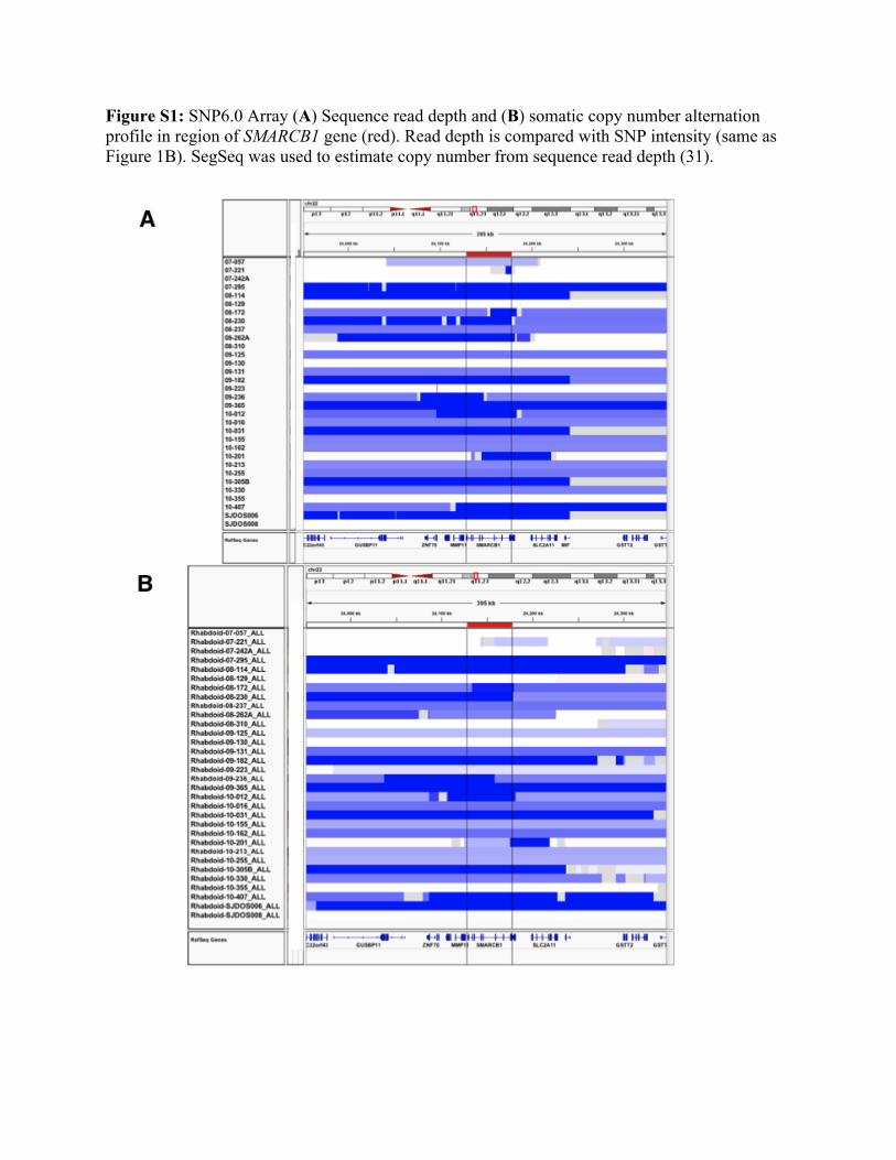
Figure S1: SNP6.0 Array (A) Sequence read depth and (B) somatic copy number alternation profile in region of SMARCB1 gene (red). Read depth is compared with SNP intensity (same as Figure 1B). SegSeq was used to estimate copy number from sequence read depth (31).

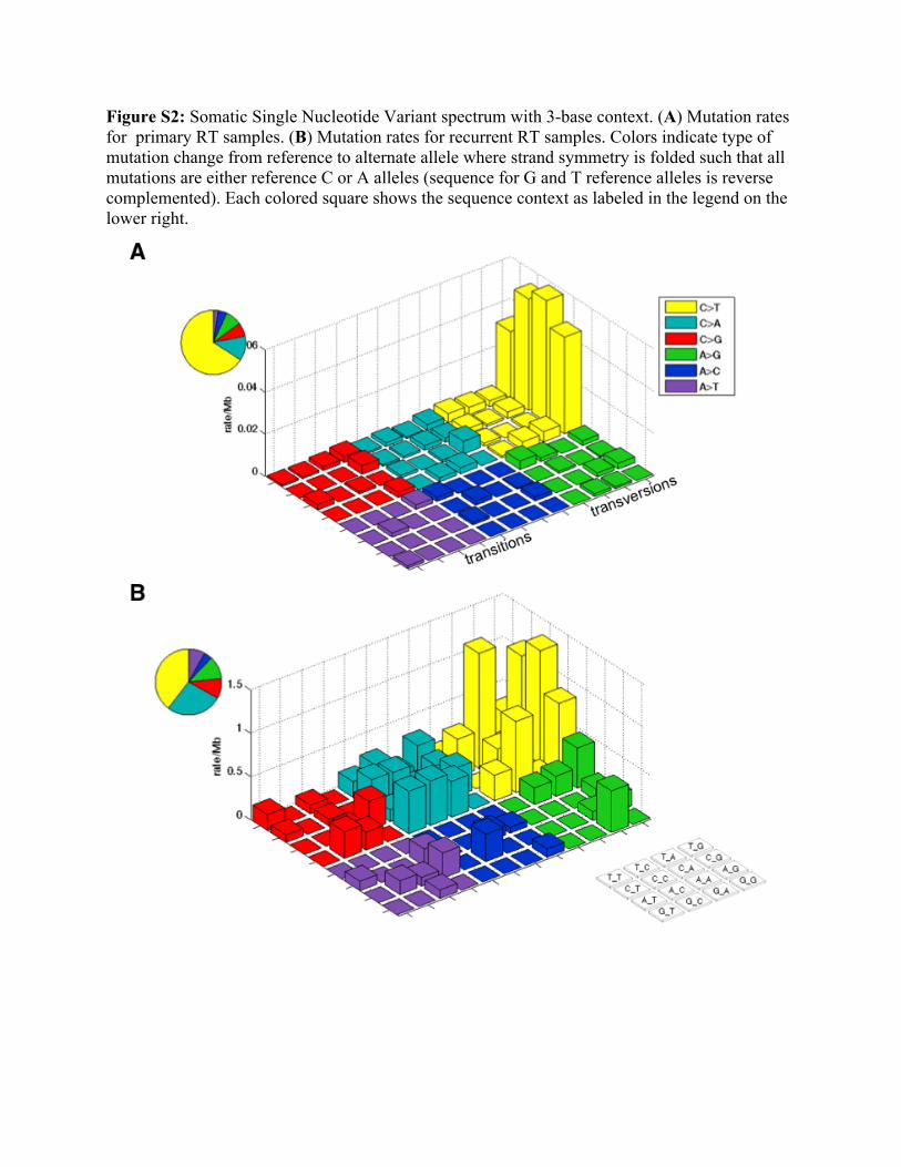
Figure S2: Somatic Single Nucleotide Variant spectrum with 3-base context. (A) Mutation rates for primary RT samples. (B) Mutation rates for recurrent RT samples. Colors indicate type of mutation change from reference to alternate allele where strand symmetry is folded such that all mutations are either reference C or A alleles (sequence for G and T reference alleles is reverse complemented). Each colored square shows the sequence context as labeled in the legend on the lower right.

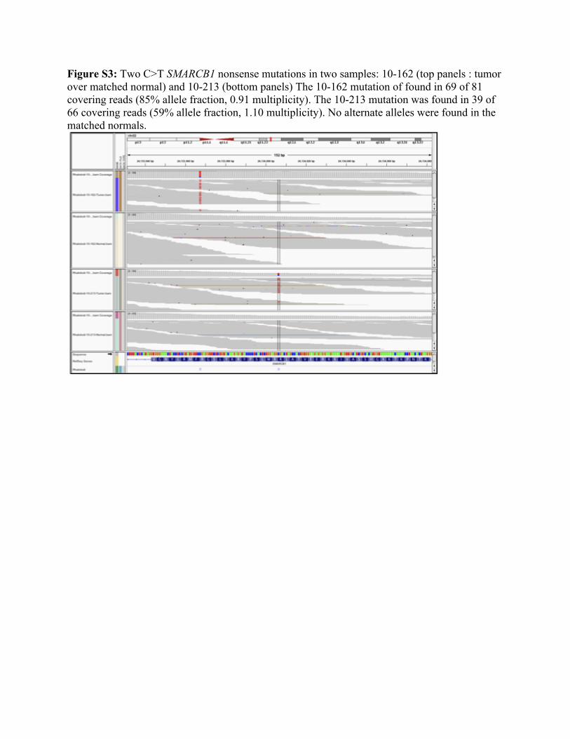
Figure S3: Two C>T SMARCB1 nonsense mutations in two samples: 10-162 (top panels : tumor over matched normal) and 10-213 (bottom panels) The 10-162 mutation of found in 69 of 81 covering reads (85% allele fraction, 0.91 multiplicity). The 10-213 mutation was found in 39 of 66 covering reads (59% allele fraction, 1.10 multiplicity). No alternate alleles were found in the matched normals.

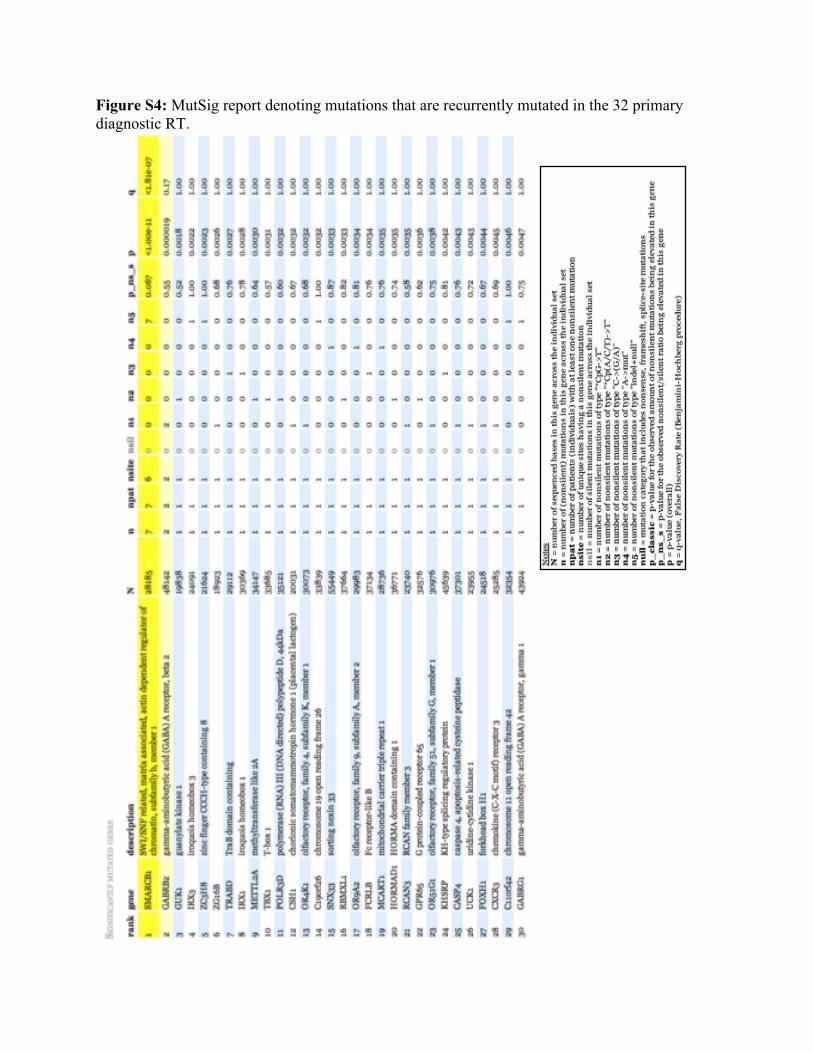
Figure S4: MutSig report denoting mutations that are recurrently mutated in the 32 primary diagnostic RT.

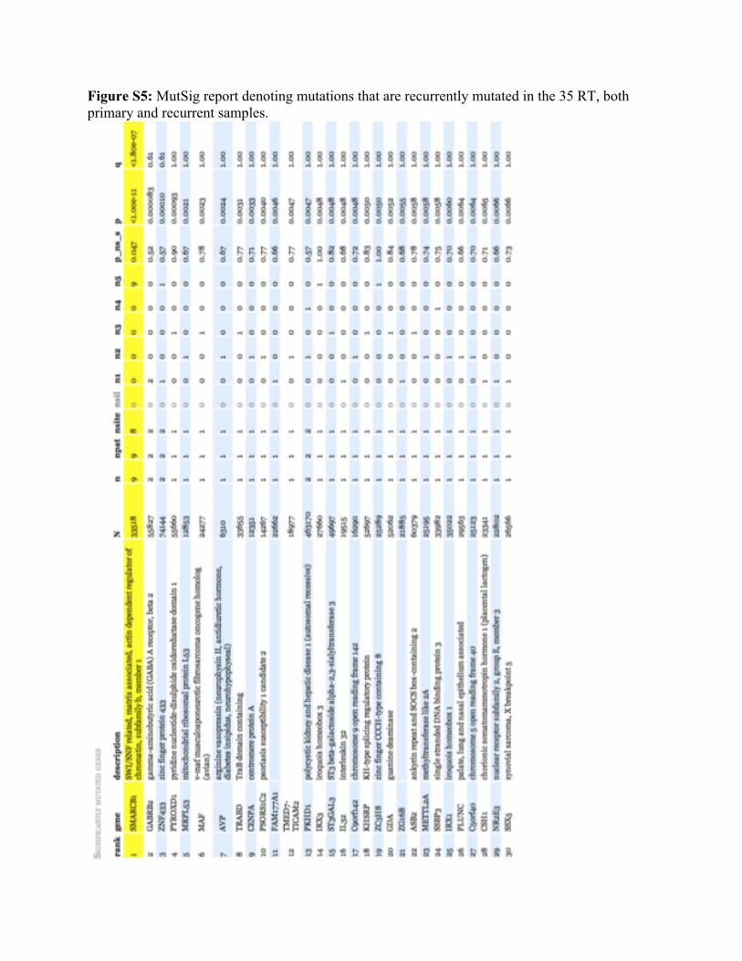
Figure S5: MutSig report denoting mutations that are recurrently mutated in the 35 RT, both primary and recurrent samples.

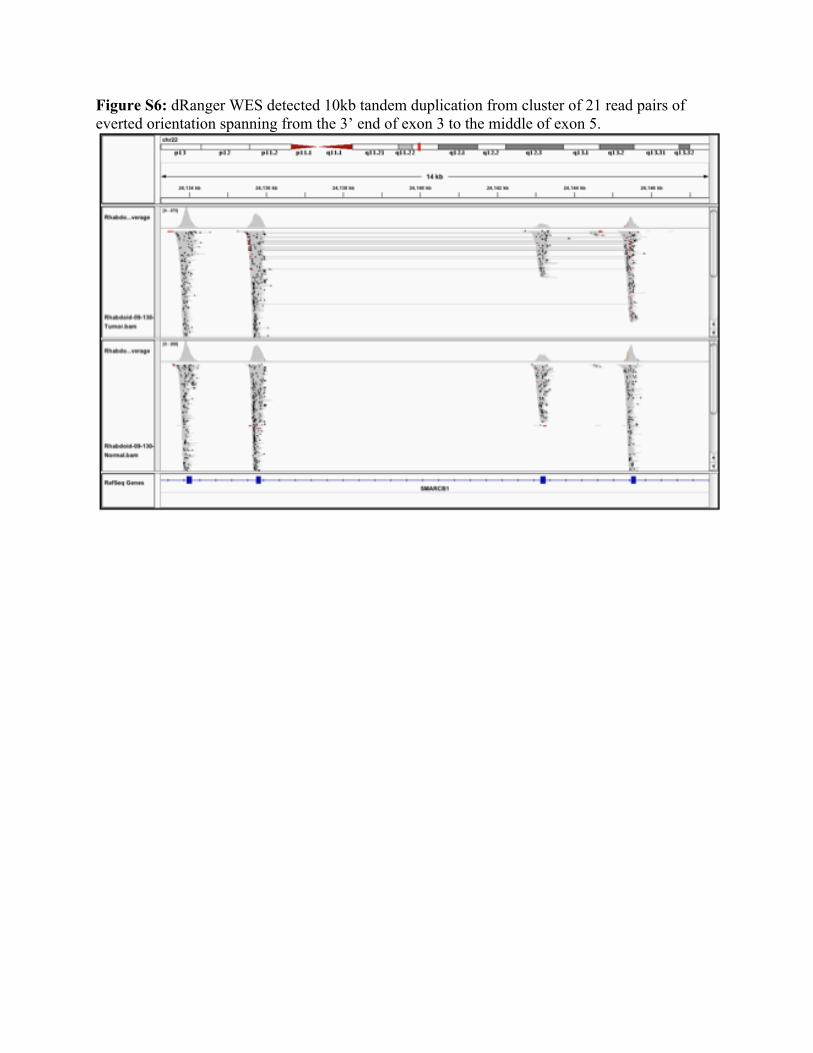
Figure S6: dRanger WES detected 10kb tandem duplication from cluster of 21 read pairs of everted orientation spanning from the 3’ end of exon 3 to the middle of exon 5.

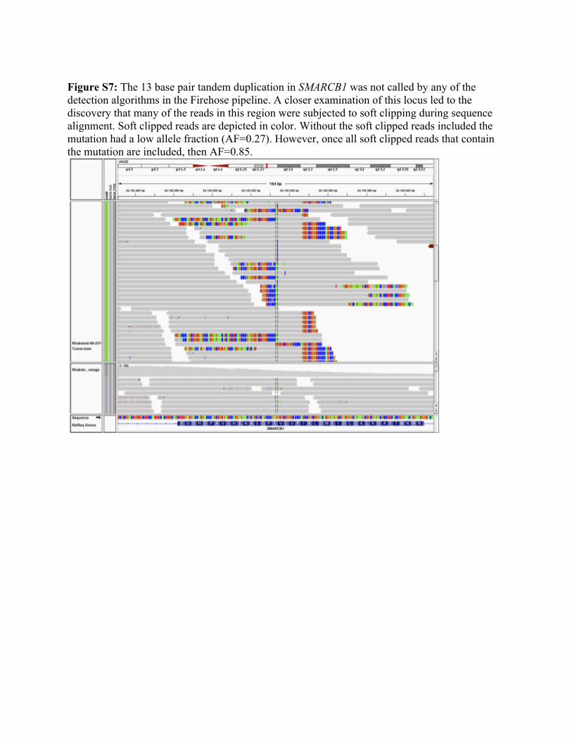
Figure S7: The 13 base pair tandem duplication in SMARCB1 was not called by any of the detection algorithms in the Firehose pipeline. A closer examination of this locus led to the discovery that many of the reads in this region were subjected to soft clipping during sequence alignment. Soft clipped reads are depicted in color. Without the soft clipped reads included the mutation had a low allele fraction (AF=0.27). However, once all soft clipped reads that contain the mutation are included, then AF=0.85.

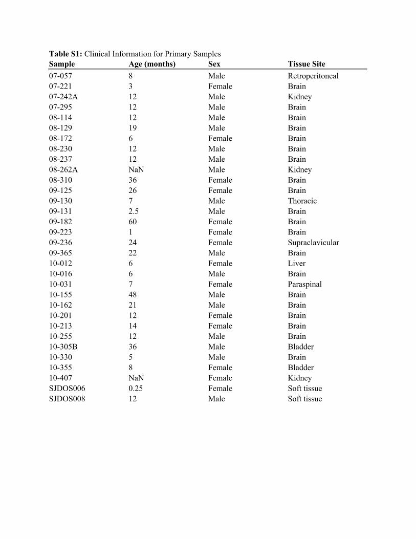
Table S1: Clinical Information for Primary Samples Sample Age (months) Sex Tissue Site 07-057 8 Male Retroperitoneal 07-221 3 Female Brain 07-242A 12 Male Kidney 07-295 12 Male Brain 08-114 12 Male Brain 08-129 19 Male Brain 08-172 6 Female Brain 08-230 12 Male Brain 08-237 12 Male Brain 08-262A NaN Male Kidney 08-310 36 Female Brain 09-125 26 Female Brain 09-130 7 Male Thoracic 09-131 2.5 Male Brain 09-182 60 Female Brain 09-223 1 Female Brain 09-236 24 Female Supraclavicular 09-365 22 Male Brain 10-012 6 Female Liver 10-016 6 Male Brain 10-031 7 Female Paraspinal 10-155 48 Male Brain 10-162 21 Male Brain 10-201 12 Female Brain 10-213 14 Female Brain 10-255 12 Male Brain 10-305B 36 Male Bladder 10-330 5 Male Brain 10-355 8 Female Bladder 10-407 NaN Female Kidney SJDOS006 0.25 Female Soft tissue SJDOS008 12 Male Soft tissue

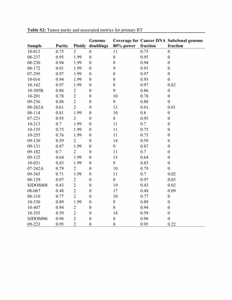
Table S2: Tumor purity and associated metrics for primary RT

Sample Purity Ploidy Genome doublings

Coverage for 80% power

Cancer DNA fraction

Subclonal genome fraction

10-012 0.75 2 0 11 0.75 0 08-237 0.95 1.99 0 8 0.95 0 08-230 0.94 1.99 0 8 0.94 0 08-172 0.91 1.99 0 9 0.91 0 07-295 0.97 1.99 0 8 0.97 0 10-016 0.94 1.99 0 8 0.93 0 10-162 0.97 1.99 0 8 0.97 0.02 10-305B 0.86 2 0 9 0.86 0 10-201 0.78 2 0 10 0.78 0 09-236 0.88 2 0 9 0.88 0 08-262A 0.61 2 0 13 0.61 0.01 08-114 0.81 1.99 0 10 0.8 0 07-221 0.95 2 0 8 0.95 0 10-213 0.7 1.99 0 11 0.7 0 10-155 0.75 1.99 0 11 0.75 0 10-255 0.76 1.99 0 11 0.75 0 09-130 0.59 2 0 14 0.59 0 09-131 0.87 1.99 0 9 0.87 0 09-182 0.7 2 0 11 0.7 0 09-125 0.64 1.99 0 13 0.64 0 10-031 0.83 1.99 0 9 0.83 0 07-242A 0.79 2 0 10 0.79 0 09-365 0.71 1.99 0 11 0.7 0.02 08-129 0.97 2 0 8 0.97 0.03 SJDOS008 0.43 2 0 19 0.43 0.02 08-067 0.48 2 0 17 0.48 0.09 08-310 0.77 2 0 10 0.77 0 10-330 0.89 1.99 0 9 0.89 0 10-407 0.94 2 0 8 0.94 0 10-355 0.59 2 0 14 0.59 0 SJDOS006 0.96 2 0 8 0.96 0 09-223 0.95 2 0 8 0.95 0.22

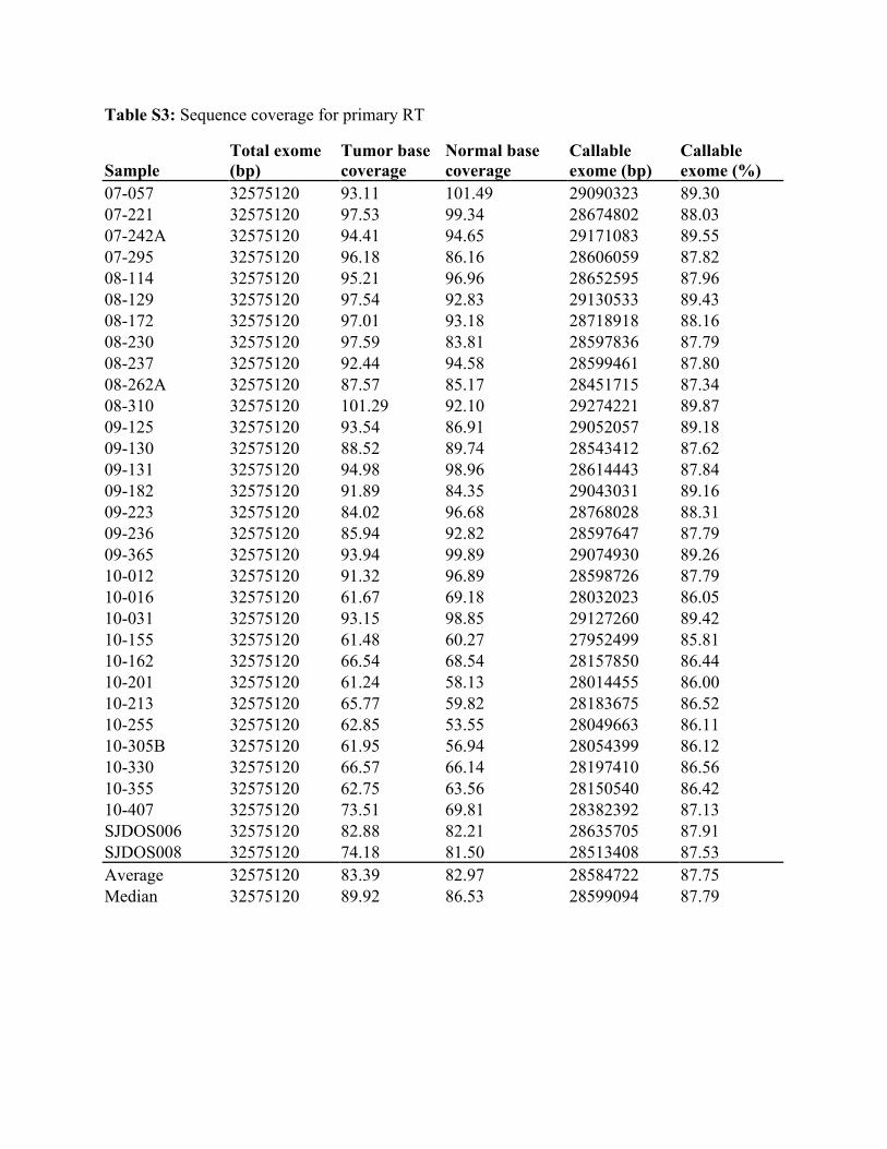
Table S3: Sequence coverage for primary RT

Sample Total exome (bp)

Tumor base coverage

Normal base coverage

Callable exome (bp)

Callable exome (%)

07-057 32575120 93.11 101.49 29090323 89.30 07-221 32575120 97.53 99.34 28674802 88.03 07-242A 32575120 94.41 94.65 29171083 89.55 07-295 32575120 96.18 86.16 28606059 87.82 08-114 32575120 95.21 96.96 28652595 87.96 08-129 32575120 97.54 92.83 29130533 89.43 08-172 32575120 97.01 93.18 28718918 88.16 08-230 32575120 97.59 83.81 28597836 87.79 08-237 32575120 92.44 94.58 28599461 87.80 08-262A 32575120 87.57 85.17 28451715 87.34 08-310 32575120 101.29 92.10 29274221 89.87 09-125 32575120 93.54 86.91 29052057 89.18 09-130 32575120 88.52 89.74 28543412 87.62 09-131 32575120 94.98 98.96 28614443 87.84 09-182 32575120 91.89 84.35 29043031 89.16 09-223 32575120 84.02 96.68 28768028 88.31 09-236 32575120 85.94 92.82 28597647 87.79 09-365 32575120 93.94 99.89 29074930 89.26 10-012 32575120 91.32 96.89 28598726 87.79 10-016 32575120 61.67 69.18 28032023 86.05 10-031 32575120 93.15 98.85 29127260 89.42 10-155 32575120 61.48 60.27 27952499 85.81 10-162 32575120 66.54 68.54 28157850 86.44 10-201 32575120 61.24 58.13 28014455 86.00 10-213 32575120 65.77 59.82 28183675 86.52 10-255 32575120 62.85 53.55 28049663 86.11 10-305B 32575120 61.95 56.94 28054399 86.12 10-330 32575120 66.57 66.14 28197410 86.56 10-355 32575120 62.75 63.56 28150540 86.42 10-407 32575120 73.51 69.81 28382392 87.13 SJDOS006 32575120 82.88 82.21 28635705 87.91 SJDOS008 32575120 74.18 81.50 28513408 87.53 Average 32575120 83.39 82.97 28584722 87.75 Median 32575120 89.92 86.53 28599094 87.79

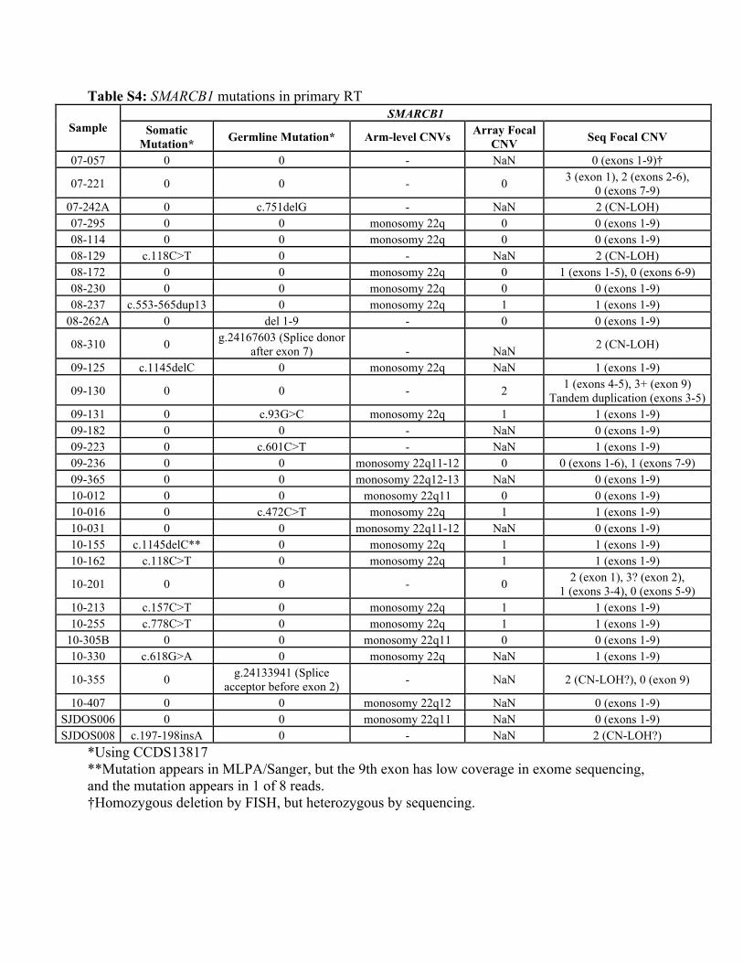
Table S4: SMARCB1 mutations in primary RT SMARCB1

Sample Somatic Mutation* Germline Mutation* Arm-level CNVs Array Focal

CNV Seq Focal CNV

07-057 0 0 - NaN 0 (exons 1-9)†

07-221 0 0 - 0 3 (exon 1), 2 (exons 2-6), 0 (exons 7-9)

07-242A 0 c.751delG - NaN 2 (CN-LOH) 07-295 0 0 monosomy 22q 0 0 (exons 1-9) 08-114 0 0 monosomy 22q 0 0 (exons 1-9) 08-129 c.118C>T 0 - NaN 2 (CN-LOH) 08-172 0 0 monosomy 22q 0 1 (exons 1-5), 0 (exons 6-9) 08-230 0 0 monosomy 22q 0 0 (exons 1-9) 08-237 c.553-565dup13 0 monosomy 22q 1 1 (exons 1-9)

08-262A 0 del 1-9 - 0 0 (exons 1-9)

08-310 0 g.24167603 (Splice donor after exon 7) - NaN 2 (CN-LOH)

09-125 c.1145delC 0 monosomy 22q NaN 1 (exons 1-9)

09-130 0 0 - 2 1 (exons 4-5), 3+ (exon 9) Tandem duplication (exons 3-5)

09-131 0 c.93G>C monosomy 22q 1 1 (exons 1-9) 09-182 0 0 - NaN 0 (exons 1-9) 09-223 0 c.601C>T - NaN 1 (exons 1-9) 09-236 0 0 monosomy 22q11-12 0 0 (exons 1-6), 1 (exons 7-9) 09-365 0 0 monosomy 22q12-13 NaN 0 (exons 1-9) 10-012 0 0 monosomy 22q11 0 0 (exons 1-9) 10-016 0 c.472C>T monosomy 22q 1 1 (exons 1-9) 10-031 0 0 monosomy 22q11-12 NaN 0 (exons 1-9) 10-155 c.1145delC** 0 monosomy 22q 1 1 (exons 1-9) 10-162 c.118C>T 0 monosomy 22q 1 1 (exons 1-9)

10-201 0 0 - 0 2 (exon 1), 3? (exon 2), 1 (exons 3-4), 0 (exons 5-9)

10-213 c.157C>T 0 monosomy 22q 1 1 (exons 1-9) 10-255 c.778C>T 0 monosomy 22q 1 1 (exons 1-9)

10-305B 0 0 monosomy 22q11 0 0 (exons 1-9) 10-330 c.618G>A 0 monosomy 22q NaN 1 (exons 1-9)

10-355 0 g.24133941 (Splice acceptor before exon 2) - NaN 2 (CN-LOH?), 0 (exon 9)

10-407 0 0 monosomy 22q12 NaN 0 (exons 1-9) SJDOS006 0 0 monosomy 22q11 NaN 0 (exons 1-9) SJDOS008 c.197-198insA 0 - NaN 2 (CN-LOH?)

*Using CCDS13817 **Mutation appears in MLPA/Sanger, but the 9th exon has low coverage in exome sequencing, and the mutation appears in 1 of 8 reads. †Homozygous deletion by FISH, but heterozygous by sequencing.

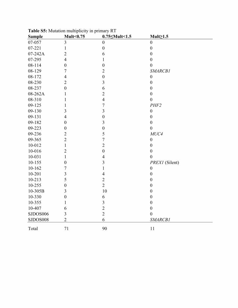
Table S5: Mutation multiplicity in primary RT Sample Mult<0.75 0.75≤Mult<1.5 Mult≥1.5 07-057 3 0 0 07-221 1 0 0 07-242A 2 6 0 07-295 4 1 0 08-114 0 0 0 08-129 7 2 SMARCB1 08-172 4 0 0 08-230 2 3 0 08-237 0 6 0 08-262A 1 2 0 08-310 1 4 0 09-125 1 7 PHF2 09-130 3 3 0 09-131 4 0 0 09-182 0 3 0 09-223 0 0 0 09-236 2 5 MUC4 09-365 2 7 0 10-012 1 2 0 10-016 2 0 0 10-031 1 4 0 10-155 0 3 PREX1 (Silent) 10-162 7 1 0 10-201 3 4 0 10-213 5 2 0 10-255 0 2 0 10-305B 3 10 0 10-330 0 6 0 10-355 1 3 0 10-407 6 2 0 SJDOS006 3 2 0 SJDOS008 2 6 SMARCB1

Total 71 90 11

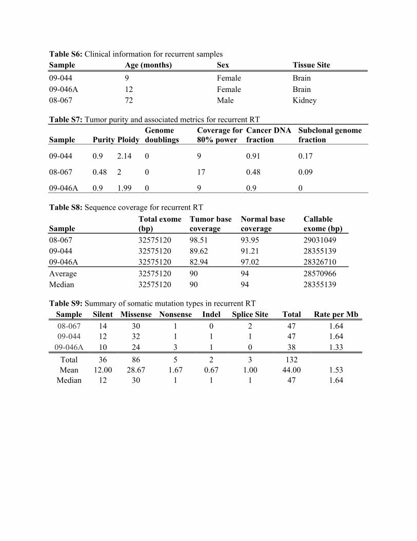
Table S6: Clinical information for recurrent samples Sample Age (months) Sex Tissue Site 09-044 9 Female Brain 09-046A 12 Female Brain 08-067 72 Male Kidney Table S7: Tumor purity and associated metrics for recurrent RT

Sample Purity Ploidy Genome doublings

Coverage for 80% power

Cancer DNA fraction

Subclonal genome fraction

09-044 0.9 2.14 0 9 0.91 0.17

08-067 0.48 2 0 17 0.48 0.09

09-046A 0.9 1.99 0 9 0.9 0 Table S8: Sequence coverage for recurrent RT

Sample Total exome (bp)

Tumor base coverage

Normal base coverage

Callable exome (bp)

08-067 32575120 98.51 93.95 29031049 09-044 32575120 89.62 91.21 28355139 09-046A 32575120 82.94 97.02 28326710 Average 32575120 90 94 28570966 Median 32575120 90 94 28355139 Table S9: Summary of somatic mutation types in recurrent RT

Sample Silent Missense Nonsense Indel Splice Site Total Rate per Mb 08-067 14 30 1 0 2 47 1.64 09-044 12 32 1 1 1 47 1.64

09-046A 10 24 3 1 0 38 1.33 Total 36 86 5 2 3 132 Mean 12.00 28.67 1.67 0.67 1.00 44.00 1.53

Median 12 30 1 1 1 47 1.64

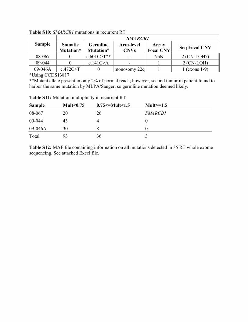
Table S10: SMARCB1 mutations in recurrent RT SMARCB1

Sample Somatic Mutation*

Germline Mutation*

Arm-level CNVs

Array Focal CNV Seq Focal CNV

08-067 0 c.601C>T** - NaN 2 (CN-LOH?) 09-044 0 c.141C>A - 1 2 (CN-LOH)

09-046A c.472C>T 0 monosomy 22q 1 1 (exons 1-9) *Using CCDS13817 **Mutant allele present in only 2% of normal reads; however, second tumor in patient found to harbor the same mutation by MLPA/Sanger, so germline mutation deemed likely. Table S11: Mutation multiplicity in recurrent RT Sample Mult<0.75 0.75<=Mult<1.5 Mult>=1.5 08-067 20 26 SMARCB1 09-044 43 4 0 09-046A 30 8 0 Total 93 36 3 Table S12: MAF file containing information on all mutations detected in 35 RT whole exome sequencing. See attached Excel file.