Support-Vector Networks - SMU

Machine Learning, 20, 273-297 (1995)© 1995 Kluwer Academic Publishers, Boston. Manufactured in The Netherlands.

Support-Vector Networks

CORINNA CORTES [email protected] VAPNIK [email protected]&T Bell Labs., Holmdel, NJ 07733, USA

Editor: Lorenza Saitta

Abstract. The support-vector network is a new learning machine for two-group classification problems. Themachine conceptually implements the following idea: input vectors are non-linearly mapped to a very high-dimension feature space. In this feature space a linear decision surface is constructed. Special properties of thedecision surface ensures high generalization ability of the learning machine. The idea behind the support-vectornetwork was previously implemented for the restricted case where the training data can be separated withouterrors. We here extend this result to non-separable training data.

High generalization ability of support-vector networks utilizing polynomial input transformations is demon-strated. We also compare the performance of the support-vector network to various classical learning algorithmsthat all took part in a benchmark study of Optical Character Recognition.

Keywords: pattern recognition, efficient learning algorithms, neural networks, radial basis function classifiers,polynomial classifiers.

1. Introduction

More than 60 years ago R.A. Fisher (Fisher, 1936) suggested the first algorithm for patternrecognition. He considered a model of two normal distributed populations, N(m 1 , EI)and N(m 2 , E2) of n dimensional vectors x with mean vectors m1 and m2 and co-variancematrices E1 and E2, and showed that the optimal (Bayesian) solution is a quadratic decisionfunction:

In the case where E1 = E2 = E the quadratic decision function (1) degenerates to a linearfunction:

To estimate the quadratic decision function one has to determine "("+3) free parameters. Toestimate the linear function only n free parameters have to be determined. In the case wherethe number of observations is small (say less than 10n2) estimating o(n2) parameters is notreliable. Fisher therefore recommended, even in the case of EI ^ £2, to use the lineardiscriminator function (2) with £ of the form:

where T is some constant1. Fisher also recommended a linear decision function for thecase where the two distributions are not normal. Algorithms for pattern recognition

274 CORTES AND VAPNIK

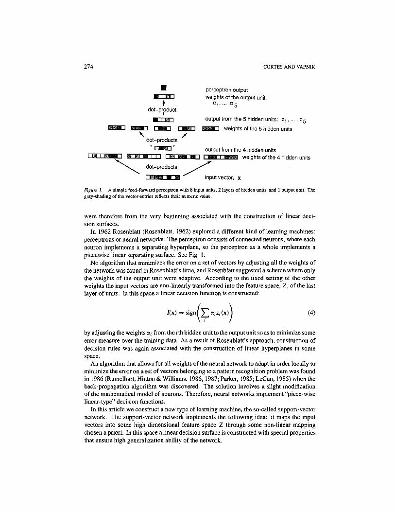
Figure 1. A simple feed-forward perceptron with 8 input units, 2 layers of hidden units, and 1 output unit. Thegray-shading of the vector entries reflects their numeric value.

were therefore from the very beginning associated with the construction of linear deci-sion surfaces.

In 1962 Rosenblatt (Rosenblatt, 1962) explored a different kind of learning machines:perceptrons or neural networks. The perceptron consists of connected neurons, where eachneuron implements a separating hyperplane, so the perceptron as a whole implements apiecewise linear separating surface. See Fig. 1.

No algorithm that minimizes the error on a set of vectors by adjusting all the weights ofthe network was found in Rosenblatt's time, and Rosenblatt suggested a scheme where onlythe weights of the output unit were adaptive. According to the fixed setting of the otherweights the input vectors are non-linearly transformed into the feature space, Z, of the lastlayer of units. In this space a linear decision function is constructed:

by adjusting the weights ai from the ith hidden unit to the output unit so as to minimize someerror measure over the training data. As a result of Rosenblatt's approach, construction ofdecision rules was again associated with the construction of linear hyperplanes in somespace.

An algorithm that allows for all weights of the neural network to adapt in order locally tominimize the error on a set of vectors belonging to a pattern recognition problem was foundin 1986 (Rumelhart, Hinton & Williams, 1986,1987; Parker, 1985; LeCun, 1985) when theback-propagation algorithm was discovered. The solution involves a slight modificationof the mathematical model of neurons. Therefore, neural networks implement "piece-wiselinear-type" decision functions.

In this article we construct a new type of learning machine, the so-called support-vectornetwork. The support-vector network implements the following idea: it maps the inputvectors into some high dimensional feature space Z through some non-linear mappingchosen a priori. In this space a linear decision surface is constructed with special propertiesthat ensure high generalization ability of the network.

SUPPORT-VECTOR NETWORKS 275

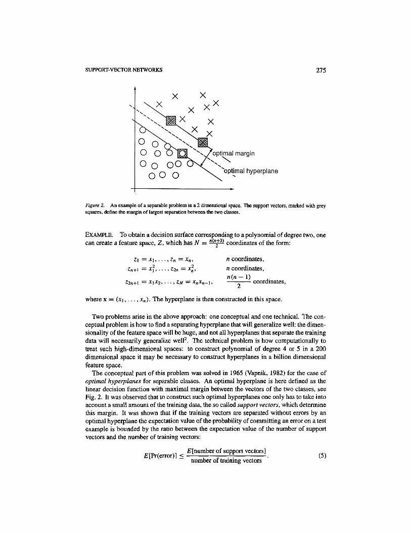
Figure 2. An example of a separable problem in a 2 dimensional space. The support vectors, marked with greysquares, define the margin of largest separation between the two classes.

EXAMPLE. To obtain a decision surface corresponding to a polynomial of degree two, onecan create a feature space, Z, which has N = 2&±21 coordinates of the form:

where x = (x\,..., xn). The hyperplane is then constructed in this space.

Two problems arise in the above approach: one conceptual and one technical. The con-ceptual problem is how to find a separating hyperplane that will generalize well: the dimen-sionality of the feature space will be huge, and not all hyperplanes that separate the trainingdata will necessarily generalize well2. The technical problem is how computationally totreat such high-dimensional spaces: to construct polynomial of degree 4 or 5 in a 200dimensional space it may be necessary to construct hyperplanes in a billion dimensionalfeature space.

The conceptual part of this problem was solved in 1965 (Vapnik, 1982) for the case ofoptimal hyperplanes for separable classes. An optimal hyperplane is here defined as thelinear decision function with maximal margin between the vectors of the two classes, seeFig. 2. It was observed that to construct such optimal hyperplanes one only has to take intoaccount a small amount of the training data, the so called support vectors, which determinethis margin. It was shown that if the training vectors are separated without errors by anoptimal hyperplane the expectation value of the probability of committing an error on a testexample is bounded by the ratio between the expectation value of the number of supportvectors and the number of training vectors:


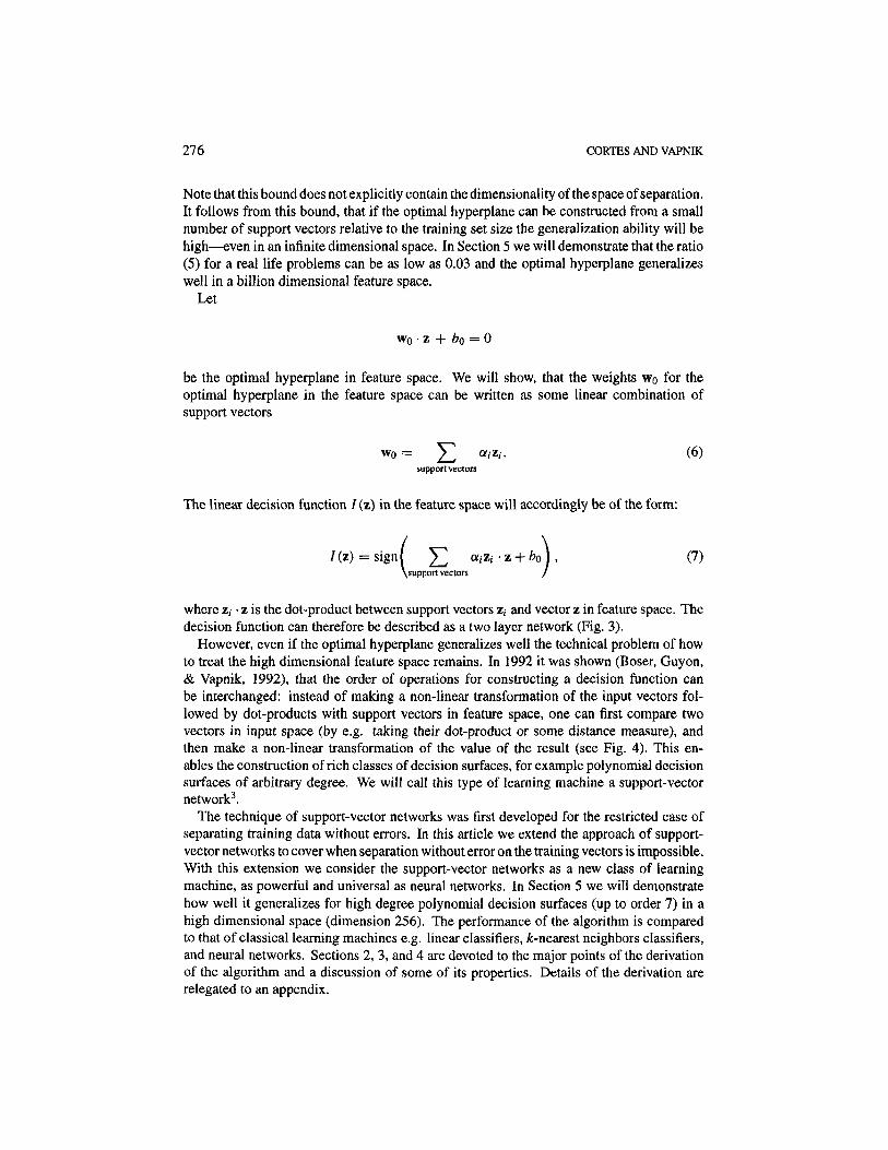
Note that this bound does not explicitly contain the dimensionality of the space of separation.It follows from this bound, that if the optimal hyperplane can be constructed from a smallnumber of support vectors relative to the training set size the generalization ability will behigh—even in an infinite dimensional space. In Section 5 we will demonstrate that the ratio(5) for a real life problems can be as low as 0.03 and the optimal hyperplane generalizeswell in a billion dimensional feature space.

Let

be the optimal hyperplane in feature space. We will show, that the weights W0 for theoptimal hyperplane in the feature space can be written as some linear combination ofsupport vectors

The linear decision function / (z) in the feature space will accordingly be of the form:

where zi- • z is the dot-product between support vectors zi and vector z in feature space. Thedecision function can therefore be described as a two layer network (Fig. 3).

However, even if the optimal hyperplane generalizes well the technical problem of howto treat the high dimensional feature space remains. In 1992 it was shown (Boser, Guyon,& Vapnik, 1992), that the order of operations for constructing a decision function canbe interchanged: instead of making a non-linear transformation of the input vectors fol-lowed by dot-products with support vectors in feature space, one can first compare twovectors in input space (by e.g. taking their dot-product or some distance measure), andthen make a non-linear transformation of the value of the result (see Fig. 4). This en-ables the construction of rich classes of decision surfaces, for example polynomial decisionsurfaces of arbitrary degree. We will call this type of learning machine a support-vectornetwork3.

The technique of support-vector networks was first developed for the restricted case ofseparating training data without errors. In this article we extend the approach of support-vector networks to cover when separation without error on the training vectors is impossible.With this extension we consider the support-vector networks as a new class of learningmachine, as powerful and universal as neural networks. In Section 5 we will demonstratehow well it generalizes for high degree polynomial decision surfaces (up to order 7) in ahigh dimensional space (dimension 256). The performance of the algorithm is comparedto that of classical learning machines e.g. linear classifiers, ̂ -nearest neighbors classifiers,and neural networks. Sections 2, 3, and 4 are devoted to the major points of the derivationof the algorithm and a discussion of some of its properties. Details of the derivation arerelegated to an appendix.


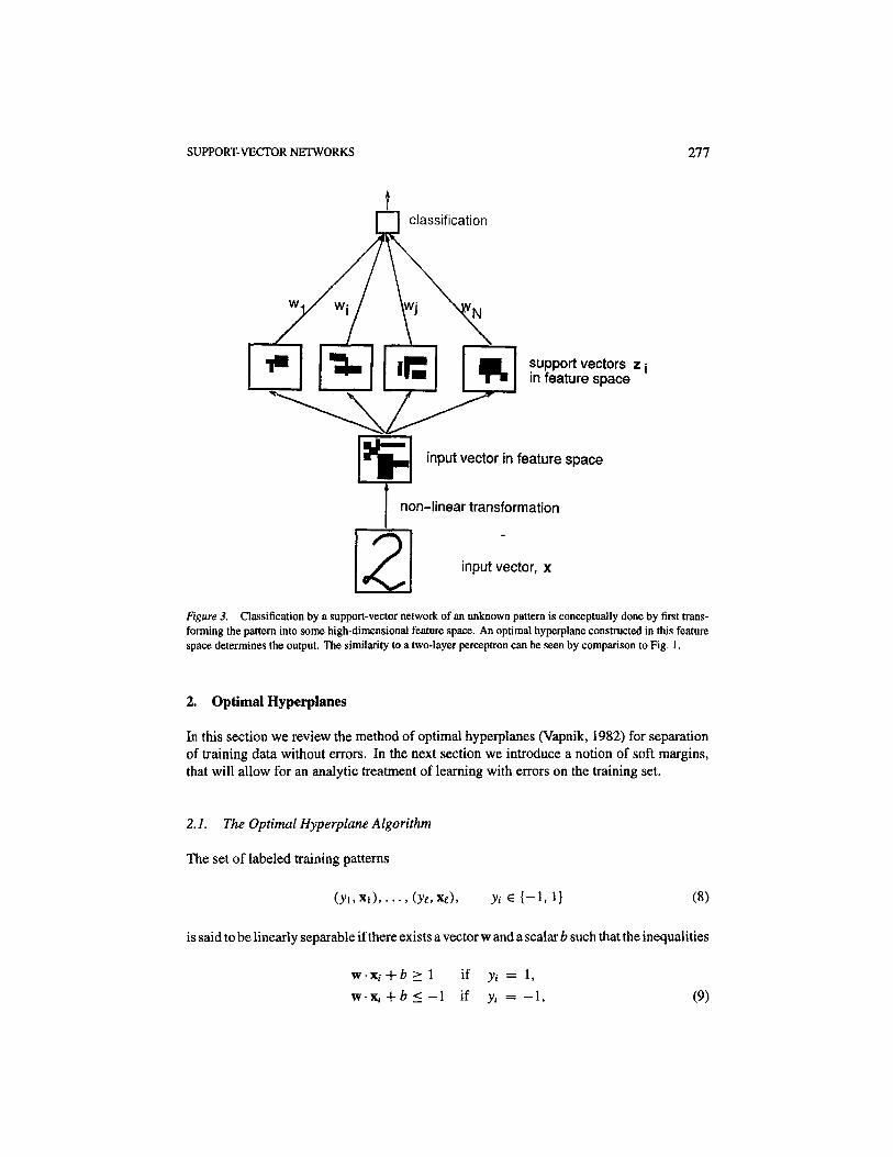
Figure 3. Classification by a support-vector network of an unknown pattern is conceptually done by first trans-forming the pattern into some high-dimensional feature space. An optimal hyperplane constructed in this featurespace determines the output. The similarity to a two-layer perceptron can be seen by comparison to Fig. 1.

2. Optimal Hyperplanes

In this section we review the method of optimal hyperplanes (Vapnik, 1982) for separationof training data without errors. In the next section we introduce a notion of soft margins,that will allow for an analytic treatment of learning with errors on the training set.

2.1. The Optimal Hyperplane Algorithm

The set of labeled training patterns

is said to be linearly separable if there exists a vector w and a scalar b such that the inequalities


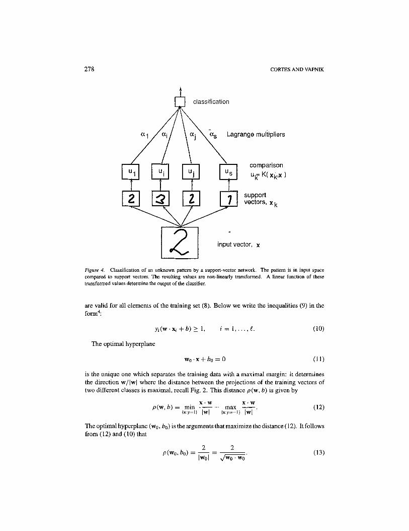
Figure 4. Classification of an unknown pattern by a support-vector network. The pattern is in input spacecompared to support vectors. The resulting values are non-linearly transformed. A linear function of thesetransformed values determine the output of the classifier.

are valid for all elements of the training set (8). Below we write the inequalities (9) in theform4:

The optimal hyperplane

is the unique one which separates the training data with a maximal margin: it determinesthe direction w/|w| where the distance between the projections of the training vectors oftwo different classes is maximal, recall Fig. 2. This distance p ( w , b) is given by

The optimal hyperplane (W0, b0) is the arguments that maximize the distance (12). It followsfrom (12) and (10) that


This means that the optimal hyperplane is the unique one that minimizes w • w under theconstraints (10). Constructing an optimal hyperplane is therefore a quadratic programmingproblem.

Vectors xi for which yi (w • x, + 6) = 1 will be termed support vectors. In Appendix A. 1we show that the vector WQ that determines the optimal hyperplane can be written as a linearcombination of training vectors:

where a° > 0. Since a > 0 only for support vectors (see Appendix), the expression (14)represents a compact form of writing w0. We also show that to find the vector of parametersai:

one has to solve the following quadratic programming problem:

with respect to Ar = (a1,... , at), subject to the constraints:

where 1T = (1 , . . . , 1) is an -dimensional unit vector, Yr = (yi y^) is the £-dimen-sional vector of labels, and D is a symmetric I x ^-matrix with elements

The inequality (16) describes the nonnegative quadrant. We therefore have to maximize thequadratic form (15) in the nonnegative quadrant, subject to the constraints (17).

When the training data (8) can be separated without errors we also show in Appendix Athe following relationship between the maximum of the functional (15), the pair (Ao, b0),and the maximal margin po from (13):

If for some A* and large constant W0 the inequality

is valid, one can accordingly assert that all hyperplanes that separate the training data (8)have a margin


If the training set (8) cannot be separated by a hyperplane, the margin between patternsof the two classes becomes arbitrary small, resulting in the value of the functional W(A)turning arbitrary large. Maximizing the functional (15) under constraints (16) and (17)one therefore either reaches a maximum (in this case one has constructed the hyperplanewith the maximal margin po), or one finds that the maximum exceeds some given (large)constant Wo (in which case a separation of the training data with a margin larger thenV^/Wo is impossible).

The problem of maximizing functional (15) under constraints (16) and (17) can be solvedvery efficiently using the following scheme. Divide the training data into a number ofportions with a reasonable small number of training vectors in each portion. Start out bysolving the quadratic programming problem determined by the first portion of training data.For this problem there are two possible outcomes: either this portion of the data cannot beseparated by a hyperplane (in which case the full set of data as well cannot be separated),or the optimal hyperplane for separating the first portion of the training data is found.

Let the vector that maximizes functional (15) in the case of separation of the first portionbe A1. Among the coordinates of vector A1 some are equal to zero. They correspond tonon-support training vectors of this portion. Make a new set of training data containingthe support vectors from the first portion of training data and the vectors of the secondportion that do not satisfy constraint (10), where w is determined by A1. For this set anew functional W2(A) is constructed and maximized at A2. Continuing this process ofincrementally constructing a solution vector A* covering all the portions of the trainingdata one either finds that it is impossible to separate the training set without error, or oneconstructs the optimal separating hyperplane for the full data set, A, = A0-. Note, thatduring this process the value of the functional W(A) is monotonically increasing, sincemore and more training vectors are considered in the optimization, leading to a smaller andsmaller separation between the two classes.

3. The Soft Margin Hyperplane

Consider the case where the training data cannot be separated without error. In this caseone may want to separate the training set with a minimal number of errors. To express thisformally let us introduce some non-negative variables £,- > 0, i = I,...,(,.

We can now minimize the functional

for small a > 0, subject to the constraints

For sufficiently small a the functional (21) describes the number of the training errors5.Minimizing (21) one finds some minimal subset of training errors:


If these data are excluded from the training set one can separate the remaining part of thetraining set without errors. To separate the remaining part of the training data one canconstruct an optimal separating hyperplane.

This idea can be expressed formally as: minimize the functional

subject to constraints (22) and (23), where F(u) is a monotonic convex function and C isa constant.

For sufficiently large C and sufficiently small a, the vector wo and constant b0, thatminimize the functional (24) under constraints (22) and (23), determine the hyperplanethat minimizes the number of errors on the training set and separate the rest of the elementswith maximal margin.

Note, however, that the problem of constructing a hyperplane which minimizes thenumber of errors on the training set is in general NP-complete. To avoid NP-completenessof our problem we will consider the case of a — 1 (the smallest value of a for whichthe optimization problem (15) has a unique solution). In this case the functional (24)describes (for sufficiently large C) the problem of constructing a separating hyperplanewhich minimizes the sum of deviations, £, of training errors and maximizes the marginfor the correctly classified vectors. If the training data can be separated without errors theconstructed hyperplane coincides with the optimal margin hyperplane.

In contrast to the case with a < I there exists an efficient method for finding the solutionof (24) in the case of a = 1. Let us call this solution the soft margin hyperplane.

In Appendix A we consider the problem of minimizing the functional

subject to the constraints (22) and (23), where F(u) is a monotonic convex function withF(0) = 0. To simplify the formulas we only describe the case of F(u) = u2 in this section.For this function the optimization problem remains a quadratic programming problem.

In Appendix A we show that the vector w, as for the optimal hyperplane algorithm, canbe written as a linear combination of support vectors x,:

To find the vector AT = («i , . . . , at) one has to solve the dual quadratic programmingproblem of maximizing

subject to constraints


where 1, A, Y, and D are the same elements as used in the optimization problem forconstructing an optimal hyperplane, S is a scalar, and (29) describes coordinate-wise in-equalities.

Note that (29) implies that the smallest admissible value S in functional (26) is

Therefore to find a soft margin classifier one has to find a vector A that maximizes

under the constraints A > 0 and (27). This problem differs from the problem of constructingan optimal margin classifier only by the additional term with amax in the functional (30).Due to this term the solution to the problem of constructing the soft margin classifier isunique and exists for any data set.

The functional (30) is not quadratic because of the term with amax. Maximizing (30)subject to the constraints A > 0 and (27) belongs to the group of so-called convex pro-gramming problems. Therefore, to construct a soft margin classifier one can either solvethe convex programming problem in the ^-dimensional space of the parameters A, or onecan solve the quadratic programming problem in the dual t + 1 space of the parameters Aand S. In our experiments we construct the soft margin hyperplanes by solving the dualquadratic programming problem.

4. The Method of Convolution of the Dot-Product in Feature Space

The algorithms described in the previous sections construct hyperplanes in the input space.To construct a hyperplane in a feature space one first has to transform the n-dimensionalinput vector x into an //-dimensional feature vector through a choice of an N-dimensionalvector function 0:

An N dimensional linear separator w and a bias b is then constructed for the set oftransformed vectors

Classification of an unknown vector x is done by first transforming the vector to the sepa-rating space (x i-»- 0 (x)) and then taking the sign of the function

According to the properties of the soft margin classifier method the vector w can bewritten as a linear combination of support vectors (in the feature space). That means


The linearity of the dot-product implies, that the classification function / in (31) for anunknown vector x only depends on the dot-products:

The idea of constructing support-vector networks comes from considering general formsof the dot-product in a Hilbert space (Anderson & Bahadur, 1966):

According to the Hilbert-Schmidt Theory (Courant & Hilbert, 1953) any symmetricfunction K(u , v), with K(u , v) e LI, can be expanded in the form

where A, e SK and fa are eigenvalues and eigenfunctions

of the integral operator defined by the kernel K(u, v). A sufficient condition to ensure that(34) defines a dot-product in a feature space is that all the eigenvalues in the expansion (35)are positive. To guarantee that these coefficients are positive, it is necessary and sufficient(Mercer's Theorem) that the condition

is satisfied for all g such that

Functions that satisfy Mercer's theorem can therefore be used as dot-products. Aizerman,Braverman and Rozonoer (1964) consider a convolution of the dot-product in the featurespace given by function of the form

which they call Potential Functions.However, the convolution of the dot-product in feature space can be given by any function

satisfying Mercer's condition; in particular, to construct a polynomial classifier of degreed in n-dimensional input space one can use the following function


Using different dot-products K(u, v) one can construct different learning machines witharbitrary types of decision surfaces (Boser, Guyon & Vapnik, 1992). The decision surfaceof these machines has a form

where xi is the image of a support vector in input space and ai is the weight of a supportvector in the feature space.

To find the vectors xi and weights ai one follows the same solution scheme as for theoriginal optimal margin classifier or soft margin classifier. The only difference is thatinstead of matrix D (determined by (18)) one uses the matrix

5. General Features of Support-Vector Networks

5.1. Constructing the Decision Rules by Support-Vector Networks is Efficient

To construct a support-vector network decision rule one has to solve a quadratic optimizationproblem:

under the simple constraints:

where matrix

is determined by the elements of the training set, and K(u, v) is the function determiningthe convolution of the dot-products.

The solution to the optimization problem can be found efficiently by solving intermediateoptimization problems determined by the training data, that currently constitute the supportvectors. This technique is described in Section 3. The obtained optimal decision functionis unique6.

Each optimization problem can be solved using any standard techniques.

5.2. The Support-Vector Network is a Universal Machine

By changing the function K (u, v) for the convolution of the dot-product one can implementdifferent networks.


In the next section we will consider support-vector network machines that use polynomialdecision surfaces. To specify polynomials of different order d one can use the followingfunctions for convolution of the dot-product

Radial Basis Function machines with decision functions of the form

can be implemented by using convolutions of the type

In this case the support-vector network machine will construct both the centers xi of theapproximating function and the weights ai.

One can also incorporate a priori knowledge of the problem at hand by constructingspecial convolution functions. Support-vector networks are therefore a rather general classof learning machines which changes its set of decision functions simply by changing theform of the dot-product.

5.3. Support- Vector Networks and Control of Generalization Ability

To control the generalization ability of a learning machine one has to control two differentfactors: the error-rate on the training data and the capacity of the learning machine asmeasured by its VC-dimension (Vapnik, 1982). There exists a bound for the probability oferrors on the test set of the following form: with probability 1 — r; the inequality

is valid. In the bound (38) the confidence interval depends on the VC-dimension of thelearning machine, the number of elements in the training set, and the value of n.

The two factors in (38) form a trade-off: the smaller the VC-dimension of the set offunctions of the learning machine, the smaller the confidence interval, but the larger thevalue of the error frequency.

A general way for resolving this trade-off was proposed as the principle of structural riskminimization: for the given data set one has to find a solution that minimizes their sum.A particular case of structural risk minimization principle is the Occam-Razor principle:keep the first term equal to zero and minimize the second one.

It is known that the VC-dimension of the set of linear indicator functions

with fixed threshold b is equal to the dimensionality of the input space. However, theVC-dimension of the subset


(the set of functions with bounded norm of the weights) can be less than the dimensionalityof the input space and will depend on Cw.

From this point of view the optimal margin classifier method executes an Occam-Razorprinciple. It keeps the first term of (38) equal to zero (by satisfying the inequality (9))and it minimizes the second term (by minimizing the functional w • w). This minimizationprevents an over-fitting problem.

However, even in the case where the training data are separable one may obtain bettergeneralization by minimizing the confidence term in (38) even further at the expense oferrors on the training set. In the soft margin classifier method this can be done by choosingappropriate values of the parameter C. In the support-vector network algorithm one cancontrol the trade-off between complexity of decision rule and frequency of error by changingthe parameter C, even in the more general case where there exists no solution with zeroerror on the training set. Therefore the support-vector network can control both factors forgeneralization ability of the learning machine.

6. Experimental Analysis

To demonstrate the support-vector network method we conduct two types of experiments.We construct artificial sets of patterns in the plane and experiment with 2nd degree poly-nomial decision surfaces, and we conduct experiments with the real-life problem of digitrecognition.

6.1. Experiments in the Plane

Using dot-products of the form

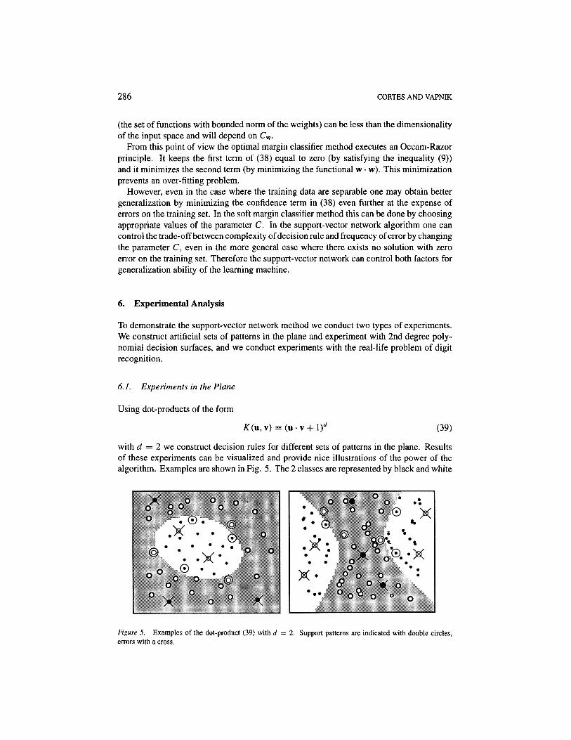
with d = 2 we construct decision rules for different sets of patterns in the plane. Resultsof these experiments can be visualized and provide nice illustrations of the power of thealgorithm. Examples are shown in Fig. 5. The 2 classes are represented by black and white

Figure 5. Examples of the dot-product (39) with d = 2. Support patterns are indicated with double circles,errors with a cross.


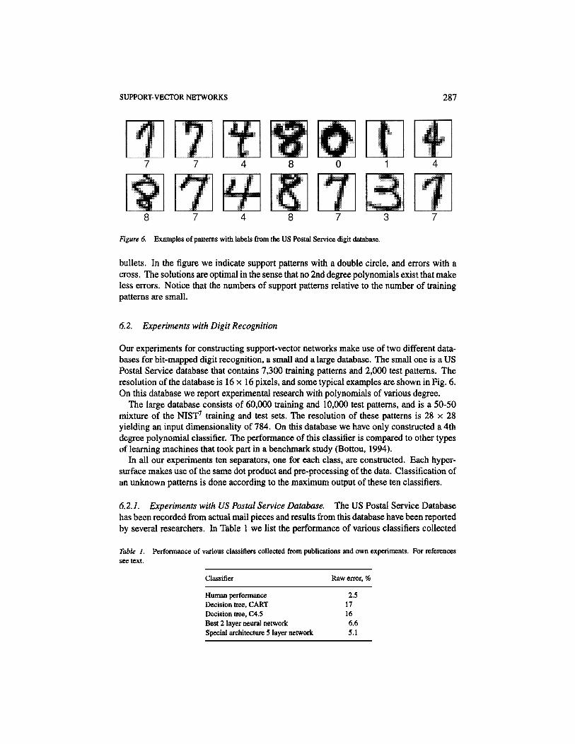
Figure 6. Examples of patterns with labels from the US Postal Service digit database.

bullets. In the figure we indicate support patterns with a double circle, and errors with across. The solutions are optimal in the sense that no 2nd degree polynomials exist that makeless errors. Notice that the numbers of support patterns relative to the number of trainingpatterns are small.

6.2. Experiments with Digit Recognition

Our experiments for constructing support-vector networks make use of two different data-bases for bit-mapped digit recognition, a small and a large database. The small one is a USPostal Service database that contains 7,300 training patterns and 2,000 test patterns. Theresolution of the database is 16 x 16 pixels, and some typical examples are shown in Fig. 6.On this database we report experimental research with polynomials of various degree.

The large database consists of 60,000 training and 10,000 test patterns, and is a 50-50mixture of the NIST7 training and test sets. The resolution of these patterns is 28 x 28yielding an input dimensionality of 784. On this database we have only constructed a 4thdegree polynomial classifier. The performance of this classifier is compared to other typesof learning machines that took part in a benchmark study (Bottou, 1994).

In all our experiments ten separators, one for each class, are constructed. Each hyper-surface makes use of the same dot product and pre-processing of the data. Classification ofan unknown patterns is done according to the maximum output of these ten classifiers.

6.2.1. Experiments with US Postal Service Database. The US Postal Service Databasehas been recorded from actual mail pieces and results from this database have been reportedby several researchers. In Table 1 we list the performance of various classifiers collected

Table 1. Performance of various classifiers collected from publications and own experiments. For referencessee text.

Classifier

Human performanceDecision tree, CARTDecision tree, C4.5Best 2 layer neural networkSpecial architecture 5 layer network

Raw error, %

2.517166.65.1


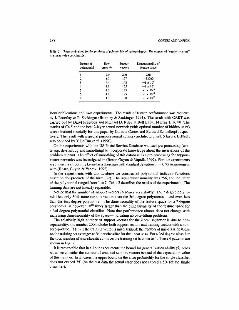
Table 2. Results obtained for dot products of polynomials of various degree. The number of "support vectors"is a mean value per classifier.

Degree ofpolynomial

1234567

Rawerror, %

12.04.74.44.34.34.24.3

Supportvectors

200127148165175185190

Dimensionality offeature space

256-33000

-1 x 106

~1 x 109

~1 x 1012

~1 x 1014

~1 x 1016

from publications and own experiments. The result of human performance was reportedby J. Bromley & E. Sackinger (Bromley & Sackinger, 1991). The result with CART wascarried out by Daryl Pregibon and Michael D. Riley at Bell Labs., Murray Hill, NJ. Theresults of C4.5 and the best 2-layer neural network (with optimal number of hidden units)were obtained specially for this paper by Corinna Cortes and Bernard Schoelkopf respec-tively. The result with a special purpose neural network architecture with 5 layers, LeNetl,was obtained by Y. LeCun et al. (1990).

On the experiments with the US Postal Service Database we used pre-processing (cen-tering, de-slanting and smoothing) to incorporate knowledge about the invariances of theproblem at hand. The effect of smoothing of this database as a pre-processing for support-vector networks was investigated in (Boser, Guyon & Vapnik, 1992). For our experimentswe chose the smoothing kernel as a Gaussian with standard deviation a = 0.75 in agreementwith (Boser, Guyon & Vapnik, 1992).

In the experiments with this database we constructed polynomial indicator functionsbased on dot-products of the form (39). The input dimensionality was 256, and the orderof the polynomial ranged from 1 to 7. Table 2 describes the results of the experiments. Thetraining data are not linearly separable.

Notice that the number of support vectors increases very slowly. The 7 degree polyno-mial has only 30% more support vectors than the 3rd degree polynomial—and even lessthan the first degree polynomial. The dimensionality of the feature space for a 7 degreepolynomial is however 1010 times larger than the dimensionality of the feature space fora 3rd degree polynomial classifier. Note that performance almost does not change withincreasing dimensionality of the space—indicating no over-fitting problems.

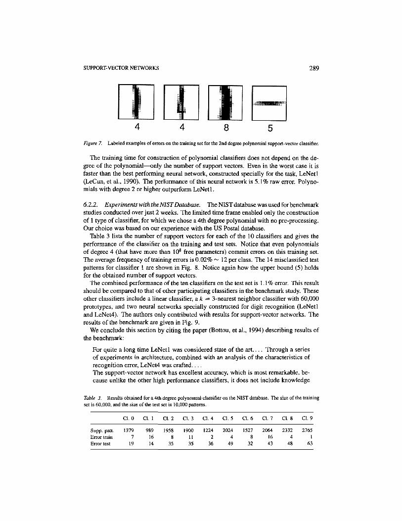
The relatively high number of support vectors for the linear separator is due to non-separability: the number 200 includes both support vectors and training vectors with a non-zero £ -value. If | > 1 the training vector is misclassified; the number of mis-classificationson the training set averages to 34 per classifier for the linear case. For a 2nd degree classifierthe total number of mis-classifications on the training set is down to 4. These 4 patterns areshown in Fig. 7.

It is remarkable that in all our experiments the bound for generalization ability (5) holdswhen we consider the number of obtained support vectors instead of the expectation valueof this number. In all cases the upper bound on the error probability for the single classifierdoes not exceed 3% (on the test data the actual error does not exceed 1.5% for the singleclassifier).


Figure 7. Labeled examples of errors on the training set for the 2nd degree polynomial support-vector classifier.

The training time for construction of polynomial classifiers does not depend on the de-gree of the polynomial—only the number of support vectors. Even in the worst case it isfaster than the best performing neural network, constructed specially for the task, LeNetl(LeCun, et al., 1990). The performance of this neural network is 5.1% raw error. Polyno-mials with degree 2 or higher outperform LeNetl.

6.2.2. Experiments with the N1ST Database. The NIST database was used for benchmarkstudies conducted over just 2 weeks. The limited time frame enabled only the constructionof 1 type of classifier, for which we chose a 4th degree polynomial with no pre-processing.Our choice was based on our experience with the US Postal database.

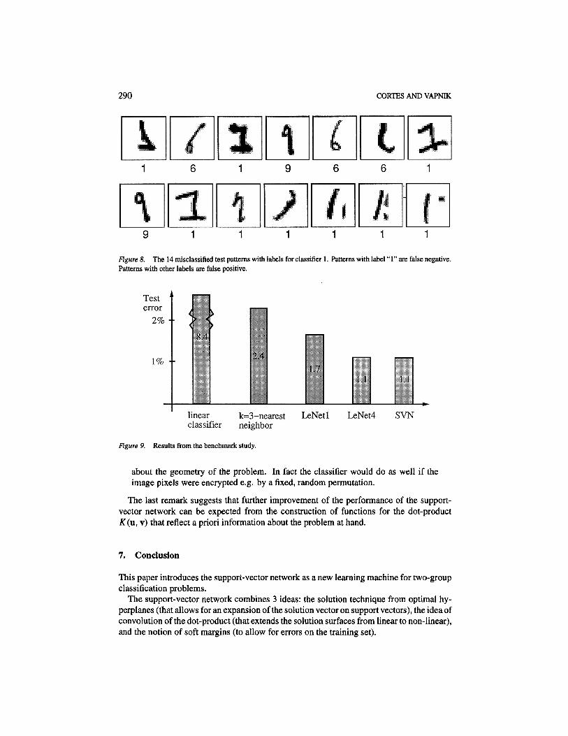
Table 3 lists the number of support vectors for each of the 10 classifiers and gives theperformance of the classifier on the training and test sets. Notice that even polynomialsof degree 4 (that have more than 108 free parameters) commit errors on this training set.The average frequency of training errors is 0.02% ~ 12 per class. The 14 misclassified testpatterns for classifier 1 are shown in Fig. 8. Notice again how the upper bound (5) holdsfor the obtained number of support vectors.

The combined performance of the ten classifiers on the test set is 1.1% error. This resultshould be compared to that of other participating classifiers in the benchmark study. Theseother classifiers include a linear classifier, a k = 3-nearest neighbor classifier with 60,000prototypes, and two neural networks specially constructed for digit recognition (LeNetland LeNet4). The authors only contributed with results for support-vector networks. Theresults of the benchmark are given in Fig. 9.

We conclude this section by citing the paper (Bottou, et al., 1994) describing results ofthe benchmark:

For quite a long time LeNetl was considered state of the art.... Through a seriesof experiments in architecture, combined with an analysis of the characteristics ofrecognition error, LeNet4 was crafted—The support-vector network has excellent accuracy, which is most remarkable, be-cause unlike the other high performance classifiers, it does not include knowledge

Table 3. Results obtained for a 4th degree polynomial classifier on the NIST database. The size of the trainingset is 60,000, and the size of the test set is 10,000 patterns.

Supp. patt.Error trainError test

C1. 0

13797

19

Cl. 1

9891614

Cl. 2

19588

35

Cl. 3

19001135

Cl. 4

12242

36

Cl. 5

20244

49

Cl. 6

15278

32

Cl. 7

20641643

Cl. 8

23324

48

Cl. 9

27651

63


Figure 8. The 14 misclassified test patterns with labels for classifier 1. Patterns with label "1" are false negative.Patterns with other labels are false positive.

Figure 9. Results from the benchmark study.

about the geometry of the problem. In fact the classifier would do as well if theimage pixels were encrypted e.g. by a fixed, random permutation.

The last remark suggests that further improvement of the performance of the support-vector network can be expected from the construction of functions for the dot-productK(u, v) that reflect a priori information about the problem at hand.

7. Conclusion

This paper introduces the support-vector network as a new learning machine for two-groupclassification problems.

The support-vector network combines 3 ideas: the solution technique from optimal hy-perplanes (that allows for an expansion of the solution vector on support vectors), the idea ofconvolution of the dot-product (that extends the solution surfaces from linear to non-linear),and the notion of soft margins (to allow for errors on the training set).


The algorithm has been tested and compared to the performance of other classical al-gorithms. Despite the simplicity of the design in its decision surface the new algorithmexhibits a very fine performance in the comparison study.

Other characteristics like capacity control and ease of changing the implemented decisionsurface render the support-vector network an extremely powerful and universal learningmachine.

A. Constructing Separating Hyperplanes

In this appendix we derive both the method for constructing optimal hyperplanes and softmargin hyperplanes.

A. 1. Optimal Hyperplane Algorithm

It was shown in Section 2, that to construct the optimal hyperplane

which separates a set of training data

one has to minimize a functional

subject to the constraints

To do this we use a standard optimization technique. We construct a Lagrangian

where Ar = (ct\,..., at) is the vector of non-negative Lagrange multipliers correspondingto the constraints (41).

It is known that the solution to the optimization problem is determined by the saddle pointof this Lagrangian in the 21 + 1-dimensional space of w, A, and b, where the minimumshould be taken with respect to the parameters w and b, and the maximum should be takenwith respect to the Lagrange multipliers A.

At the point of the minimum (with respect to w and b) one obtains:


From equality (43) we derive

which expresses, that the optimal hyperplane solution can be written as a linear combina-tion of training vectors. Note, that only training vectors x, with ai > 0 have an effectivecontribution to the sum (45).

Substituting (45) and (44) into (42) we obtain

In vector notation this can be rewritten as

where 1 is an i-dimensional unit vector, and D is a symmetric t x ^-matrix with elements

To find the desired saddle point it remains to locate the maximum of (48) under theconstraints (43)

where Yr = (y\,... ,yt), and

The Kuhn-Tucker theorem plays an important part in the theory of optimization. Ac-cording to this theorem, at our saddle point in W0, bo, A0, any Lagrange multiplier af andits corresponding constraint are connected by an equality

From this equality comes that non-zero values ai are only achieved in the cases where

In other words: ai- ^ 0 only for cases were the inequality is met as an equality. We callvectors xi for which

for support-vectors. Note, that in this terminology the Eq. (45) states that the solution vectorW0 can be expanded on support vectors.


Another observation, based on the Kuhn-Tucker Eqs. (44) and (45) for the optimalsolution, is the relationship between the maximal value W(Ao) and the separation distanceA>:

Substituting this equality into the expression (46) for W(A 0 ) we obtain

Taking into account the expression (13) from Section 2 we obtain

where po is the margin for the optimal hyperplane.

A.2. Soft Margin Hyperplane Algorithm

Below we first consider the case of F(u) = uk. Then we describe the general result for amonotonic convex function F(u).

To construct a soft margin separating hyperplane we maximize the functional

under the constraints

The Lagrange functional for this problem is

where the non-negative multipliers Ar = (a1, a2 ai) arise from the constraint (49),and the multipliers Rr = (r\, r2,.. . . , r1) enforce the constraint (50).

We have to find the saddle point of this functional (the minimum with respect to thevariables wi, b, and £,-, and the maximum with respect to the variables a, and ri).

Let us use the conditions for the minimum of this functional at the extremum point:


If we denote

we can rewrite Eq. (54) as

From the equalities (52)-(55) we find

Substituting the expressions for WQ, bo, and S into the Lagrange functional (51) we obtain

To find the soft margin hyperplane solution one has to maximize the form functional(59) under the constraints (57)-(58) with respect to the non-negative variables ai, ri with(' = 1 , . . . , / . In vector notation (59) can be rewritten as

where A and D are as defined above. To find the desired saddle point one therefore has tofind the maximum of (60) under the constraints

and

From (62) and (64) one obtains that the vector A should satisfy the conditions


From conditions (62) and (64) one can also conclude that to maximize (60)

Substituting this value of S into (60) we obtain

To find the soft margin hyperplane one can therefore either find the maximum of the quadraticform (51) under the constraints (61) and (65), or one has to find the maximum of the convexfunction (60) under the constraints (61) and (56). For the experiments reported in this paperwe used k = 2 and solved the quadratic programming problem (51).

For the case of F(u) = u the same technique brings us to the problem of solving thefollowing quadratic optimization problem: minimize the functional


and

The general solution for the case of a monotone convex function F(u) can also be obtainedfrom this technique. The soft margin hyperplane has a form

where Aj = (a°,..., o$) is the solution of the following dual convex programming prob-lem: maximize the functional


where we denote

For convex monotone functions F(u) with F(0) = 0 the following inequality is valid:

Therefore the second term in square brackets is positive and goes to infinity when Ua^ goesto infinity.


Finally, we can consider the hyperplane that minimizes the form

subject to the constraints (49)-(50), where the second term minimizes the least square valuefor the errors. This lead to the following quadratic programming problem: maximize thefunctional

in the non-negative quadrant A > 0 subject to the constraint Ar Y = 0.

Notes

1. The optimal coefficient for T was found in the sixties (Anderson & Bahadur, 1966).

2. Recall Fisher's concerns about small amounts of data and the quadratic discriminant function.

3. With this name we emphasize how crucial the idea of expanding the solution on support vectors is for theselearning machines. In the support-vectors learning algorithm the complexity of the construction does notdepend on the dimensionality of the feature space, but on the number of support vectors.

4. Note that in the inequalities (9) and (10) the right-hand side, but not vector w, is normalized.

5. A training error is here defined as a pattern where the inequality (22) holds with f > 0.

6. The decision function is unique but not its expansion on support vectors.

7. National Institute for Standards and Technology, Special Database 3.

References

Aizerman, M., Braverman, E., & Rozonoer, L. (1964). Theoretical foundations of the potential function methodin pattern recognition learning. Automation and Remote Control, 25:821-837.

Anderson, T.W., & Bahadur, R.R. (1966). Classification into two multivariate normal distributions with differentcovariance matrices. Ann. Math. Stat., 33:420-431.

Boser, B.E., Guyon, I., & Vapnik, V.N. (1992). A training algorithm for optimal margin classifiers. In Proceedingsof the Fifth Annual Workshop of Computational Learning Theory, 5, 144-152, Pittsburgh, ACM.

Bottou, L., Cortes, C, Denker, J.S., Drucker, H., Guyon, I., Jacket, L.D., LeCun, Y., Sackinger, E., Simard, P.,Vapnik, V., & Miller, U.A. (1994). Comparison of classifier methods: A case study in handwritten digitrecognition. Proceedings of 12th International Conference on Pattern Recognition and Neural Network.

Bromley, J., & Sackinger, E. (1991). Neural-network and it-nearest-neighbor classifiers. Technical Report 11359-910819-16TM, AT&T.

Courant, R., & Hilbert, D. (1953). Methods of Mathematical Physics, Interscience, New York.Fisher, R.A. (1936). The use of multiple measurements in taxonomic problems. Ann. Eugenics, 7:111-132.LeCun, Y. (1985). Une procedure d'apprentissage pour reseau a seuil assymetrique. Cognitiva 85: A la Frontiere

de I'Intelligence Artificielle des Sciences de la Connaissance des Neurosciences, 599-604, Paris.LeCun, Y, Boser, B., Denker, J.S., Henderson, D., Howard, R.E., Hubbard, W., & Jackel, L.D. (1990). Handwritten

digit recognition with a back-propagation network. Advances in Neural Information Processing Systems, 2,396-404, Morgan Kaufman.

Parker, D.B. (1985). Learning logic. Technical Report TR-47, Center for Computational Research in Economicsand Management Science, Massachusetts Institute of Technology, Cambridge, MA.

Rosenblatt, F. (1962). Principles ofNeurodynamics, Spartan Books, New York.


Rumelhart, D.E., Hinton, G.E., & Williams, R.J. (1986). Learning internal representations by backpropagatingerrors. Nature, 323:533-536.

Rumelhart, D.E., Hinton, G.E., & Williams, R.J. (1987). Learning internal representations by error propagation.In James L. McClelland & David E. Rumelhart (Eds.), Parallel Distributed Processing, 1,318-362, MIT Press.

Vapnik, V.N. (1982). Estimation of Dependences Based on Empirical Data, Addendum 1, New York: Springer-Verlag.

Received May 15, 1993Accepted February 20, 1995Final Manuscript March 8,1995

Documents

Support-Vector Networks - SMU