Surface Reconstruction by layer peeling

8/7/2019 Surface Reconstruction by layer peeling

http://slidepdf.com/reader/full/surface-reconstruction-by-layer-peeling 1/11

Visual Comput (2006) 22: 593–603DOI 10.1007/s00371-006-0048-9 O R I G I N A L A R T I C L E

Chi-Wan LimTiow-Seng Tan

Surface reconstruction by layer peeling

Published online: 24 August 2006© Springer-Verlag 2006

C.-W. Lim (u) ·T.-S. TanSchool of Computing, National Universityof Singapore, 3 Science Drive 2,Singapore 117543{limchiwa, tants}@comp.nus.edu.sg

Abstract Given an input point cloudP inR3, this paper proposes a novelalgorithm to identify surface neigh-

bors of each point p ∈ P respectingthe underlying surface S and then toconstruct a piecewise linear surfacefor P. The algorithm utilizes thesimple k -nearest neighborhood inconstructing local surfaces. It makesuse of two concepts: a local convexitycriterion to extract a set of surfaceneighbors for each point, and a globalprojection test to determine an orderfor the reconstruction. Our algorithmnot only produces a topologicallycorrect surface for well-sampled

point sets, but also adapts well tohandle under-sampled point sets.Furthermore, the computational cost

of the algorithm increases almostlinearly in the size of the point cloud.It, thus, scales well to deal with largeinput point sets.

Keywords Surface reconstruc-tion · Mesh generation · Geometricmodeling · Sampling · Scattered data

1 Introduction

Surface reconstruction from an unorganized point set isa difficult and ill-posed problem as no surface informa-tion is known and there is no unique solution. Existingwork can be categorized into three broad types with noisysampling having high sampling density at one end andunder-sampling at the other end. Most existing algorithms

focus on optimal [4] and noisy sampling types [17] thatrequire input data to be of good sampling density thatsatisfies ε-sampling criterion. Little discussion has beenmade regarding the output of these algorithms when thiscriterion is not fulfilled.

Indeed, the ε-sampling criterion may not be fulfilled inpractice as objects are more likely to be regularly sampledthan sampled at very high density. In another view, thesealgorithms frequently employed triangulation algorithms(or Voronoi diagrams) as an intermediate step. This re-

sults in non-linear computational time in general (thoughthere are special cases of triangulation that runs in lineartime [9]). It is, thus, interesting to investigate an almostlinear time surface reconstruction algorithm to deal withlarge input point clouds.

This paper proposes a novel surface reconstruction al-gorithm that runs in time almost linear to the size of theinput point cloud and is well suited to handle the case of under-sampled input. Very briefly, the algorithm employs

a layer peeling approach to uncover a surface in a layer-by-layer manner without the use of triangulation tech-niques that are global in nature. At each layer, it strives toform triangle fans for some data points in order to deter-mine their neighborhood points. These triangle fans are inturn merged to form a surface for the input.

Section 2 reviews previous work in this area and iden-tifies issues in the existing methods. Section 3 discussesthe problems that exist in reconstructing under-sampledpoint sets. Section 4 describes our proposed layer peeling



594 C.-W. Lim, T.-S. Tan

algorithm. Section 5 details the construction and mergingof triangle fans. Section 6 provides an analysis of the al-gorithm with under-sampling and with optimal samplingconditions. Section 7 details our experimental results, andSect. 8 concludes the paper.

2 Related work

Among many works in surface reconstruction, we discussin the following a few important branches of approaches.Other branches of theoretical works or with algebraicpatches and level set methods (such as [25, 27, 30, 31]) areless relevant to our work here.

The use of k -nearest neighborhood is quite commonamong many methods. The earliest such work is de-veloped by Hoppe et al. [21]. For a point p, the algorithmuses its k -nearest neighbors to compute a three-by-threecovariance matrix to locally estimate the signed distancefunction and then to generate a mesh output. Other works

such as [1, 2, 6, 22] have tried to fit implicit surfaces overthe sets of k -nearest neighborhood. Works such as [12]have tried to similarly fit radial basis functions. In gen-eral, these algorithms face difficulties during the recon-struction when the k -nearest neighborhood contains pointsfrom disjoint portions of the surface.

Another branch of global based methods uses Voronoidiagrams and Delaunay triangulations [3–5, 16]. Amentaet al. [5] used the concept of poles in Voronoi cells tohelp estimate the point normals, which are in turn usedto assist in surface reconstruction. The advantage of usingDelaunay triangulation is that it provides a platform toprove the correctness of these algorithms on ε-sampled

surfaces. However, when the ε-sampling criterion is notmet, such as in practice that point clouds are just uni-formly sampled, there is no guarantee on the output qual-ity.

Bernardini et al. [11] used a ball-pivoting algorithmto detect and form triangles to construct a surface mesh.Another such advancing-front approach is the work pro-posed by Scheidegger et al. [29]. Their work focuses onmeshing noisy point set surfaces, allowing users to se-lect an error bound. Our work is similar to their tech-niques but improves upon them by taking into considera-tion of point clouds possibly under-sampled and formingmore perceived layers (such as the point set shown in

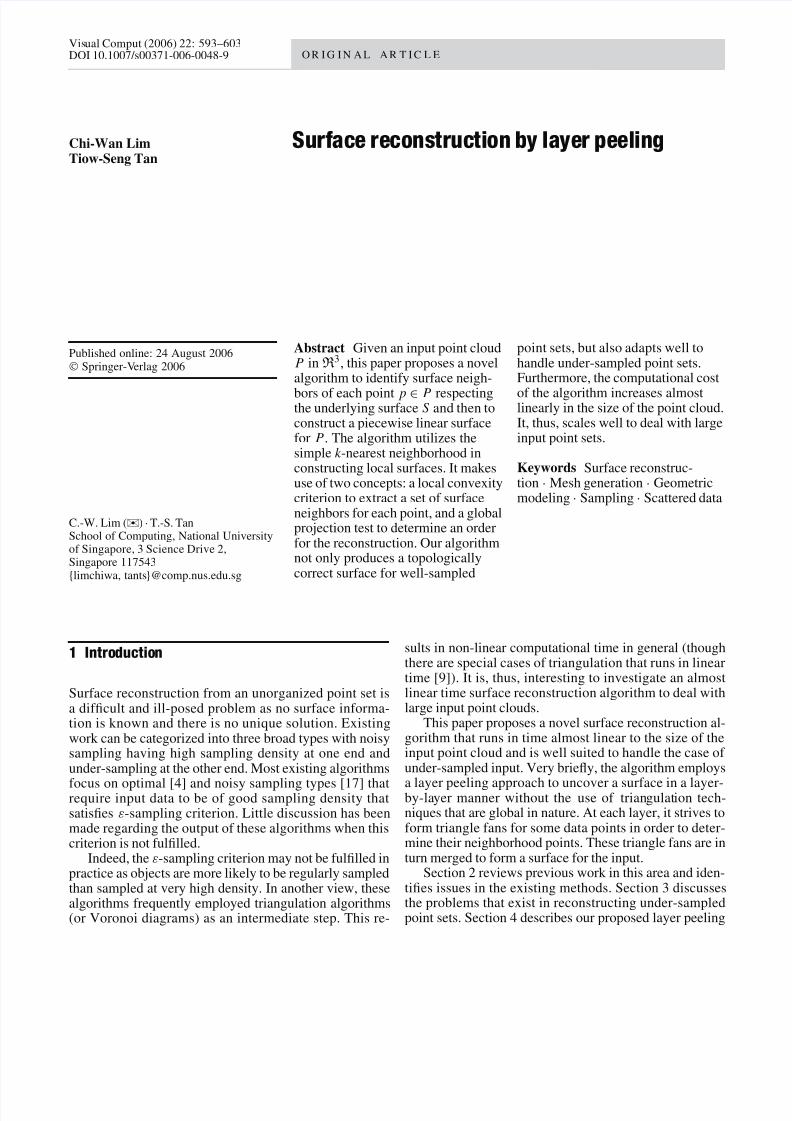
Fig. 1).Under-sampled point sets have only been briefly men-tioned in a few works, such as [14]. Their work is, how-ever, more focused towards the detection of undersam-pling, rather than adapting to the problem.

The issue of improving the timing of triangulationalgorithm has been explored. Funke and Ramos [18]provided a theoretical improvement to the Cocone algo-rithm [4] by performing a local search for possible can-didates for triangulation around a particular point. Our

Fig. 1. The layer peelingalgorithm is able to re-construct surfaces frompoint sets of complextopology

method differs from their work by using a convexity cri-terion to construct triangle fans and it runs in near lineartime in our extensive experiments. Gopi et al. [20] useda projection plane to perform a lower dimension Delau-nay triangulation within a local space. However, theirprojection plane is determined only by local eigenanaly-sis, which can be inaccurate for an under-sampled point

set.

3 Problems of under-sampled points sets

As discussed in the previous section, there are two mainways to perform surface reconstruction. The first one usesk -nearest neighbors for each point. In this case, if the k -nearest neighbors are all located around the local surfaceof the point, accurate reconstruction tends to occur. How-ever, if some of the k -nearest neighbors are from differentparts of the surface, errors during reconstruction are un-avoidable. On the other hand, the second way is a more

global approach that uses Delaunay triangulations. Still,the accuracy of a reconstruction (derived from the calcula-tion of the poles) is inevitably affected by the same issueof nearby points coming from different parts of the sur-face [4, 5].

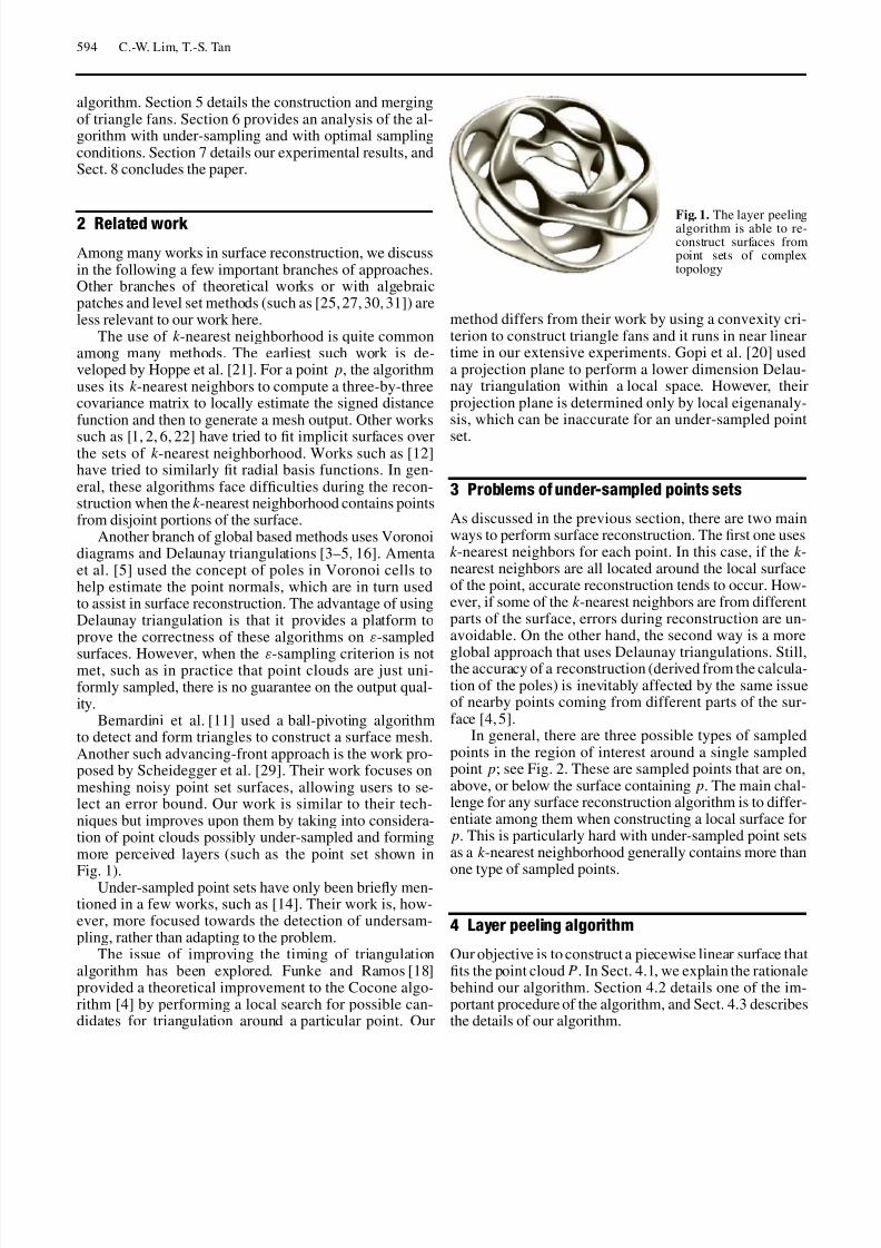
In general, there are three possible types of sampledpoints in the region of interest around a single sampledpoint p; see Fig. 2. These are sampled points that are on,above, or below the surface containing p. The main chal-lenge for any surface reconstruction algorithm is to differ-entiate among them when constructing a local surface forp. This is particularly hard with under-sampled point setsas a k -nearest neighborhood generally contains more than

one type of sampled points.

4 Layer peeling algorithm

Our objective is to construct a piecewise linear surface thatfits the point cloud P. In Sect. 4.1, we explain the rationalebehind our algorithm. Section 4.2 details one of the im-portant procedure of the algorithm, and Sect. 4.3 describesthe details of our algorithm.



Surface reconstruction by layer peeling 595

Fig. 2. The k -nearest neighbors for a point in an under-sampledpoint set can contain sampled points on the same surface, or sam-ple points from other parts of the surfaces that are below or above(shown within red ovals)

4.1 Algorithmic rationale

We begin with two simple observations about closed-manifolds in general and their influences on our algo-rithm.

Fact 1. For any closed-manifold surface in 3D that is wa-tertight and bounds a volume, a ray intersecting the sur-face is always alternating between front-facing (i.e., fromoutside the bounded volume to the inside) and back-facingintersection.

As the manifold is closed, no path exists that leads

from the inside of the bounded volume to the outside (orvice versa) without passing through the surface. Each in-tersection brings the ray from outside into the inside of the bounded volume, and another intersection is needed tobring the ray out of the bounded volume.

Fact 2. Consider a rendering of a point set using splatsor small disc at each point. For a viewpoint aligned alongthe normal of a point, the point itself is visible if, and onlyif, no splats rendered at the other points intersect with thenormal ray from the point.

In rendered images, any object closer to viewpoint oc-cludes the other. Fact 2 thus follows. With these two facts

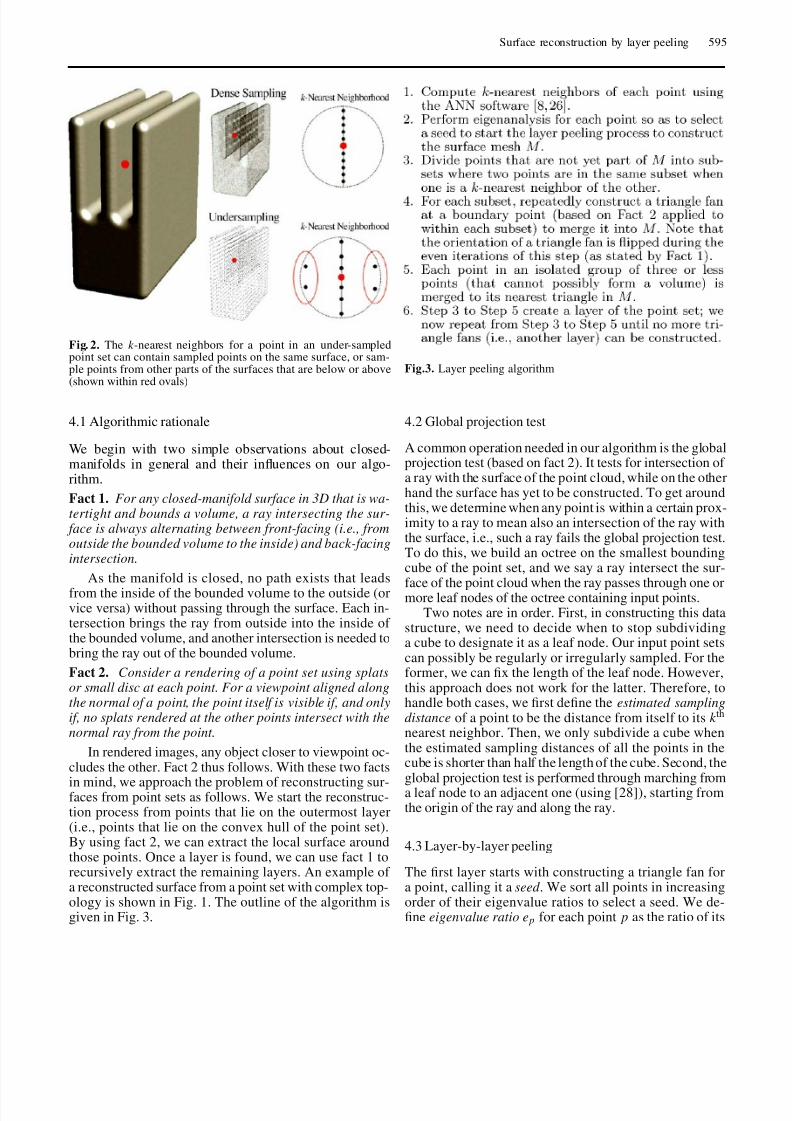
in mind, we approach the problem of reconstructing sur-faces from point sets as follows. We start the reconstruc-tion process from points that lie on the outermost layer(i.e., points that lie on the convex hull of the point set).By using fact 2, we can extract the local surface aroundthose points. Once a layer is found, we can use fact 1 torecursively extract the remaining layers. An example of a reconstructed surface from a point set with complex top-ology is shown in Fig. 1. The outline of the algorithm isgiven in Fig. 3.

Fig.3. Layer peeling algorithm

4.2 Global projection test

A common operation needed in our algorithm is the globalprojection test (based on fact 2). It tests for intersection of a ray with the surface of the point cloud, while on the otherhand the surface has yet to be constructed. To get aroundthis, we determine when any point is within a certain prox-imity to a ray to mean also an intersection of the ray withthe surface, i.e., such a ray fails the global projection test.To do this, we build an octree on the smallest boundingcube of the point set, and we say a ray intersect the sur-

face of the point cloud when the ray passes through one ormore leaf nodes of the octree containing input points.Two notes are in order. First, in constructing this data

structure, we need to decide when to stop subdividinga cube to designate it as a leaf node. Our input point setscan possibly be regularly or irregularly sampled. For theformer, we can fix the length of the leaf node. However,this approach does not work for the latter. Therefore, tohandle both cases, we first define the estimated samplingdistance of a point to be the distance from itself to its k th

nearest neighbor. Then, we only subdivide a cube whenthe estimated sampling distances of all the points in thecube is shorter than half the length of the cube. Second, theglobal projection test is performed through marching froma leaf node to an adjacent one (using [28]), starting fromthe origin of the ray and along the ray.

4.3 Layer-by-layer peeling

The first layer starts with constructing a triangle fan fora point, calling it a seed . We sort all points in increasingorder of their eigenvalue ratios to select a seed. We de-fine eigenvalue ratio ep for each point p as the ratio of its




smallest eigenvalue to the sum of all its three eigenvalues(as computed in the standard way from the covariance ma-trix defined on the k -nearest neighbors of p). However, weignore points that have two out of three eigenvalues withabnormally low values. To determine whether a point pcan be a seed, we use the ray r which is the third (smallest)eigenvector associated with p, and check whether it passes

the global projection test. If it does, p qualifies as a seedand r is assigned as its normal. Otherwise we repeat thetest for −r to determine whether p can still be a seed with−r as its normal.

We construct a triangle fan at the chosen seed (Sect. 5).This triangle fan becomes the initial mesh M for us to iter-atively select another point which is lying on the boundaryof M to form a triangle fan to merge into M . We termboundary points as points in M whose triangle fans haveyet to be constructed. There are generally many bound-ary points and thus many possible triangle fans to considerfor merging into M . As such, we prioritize all trianglefans using a heap, with preference given to one with the

smallest variance of dihedral angles where each is de-fined between a pair of triangles sharing an edge in thetriangle fan. A triangle fan can only be added to the heapif it passes the global projection test with its normal asthe test ray. Each time a triangle fan is merged to M ,the boundary of M changes with new points, and newtriangle fans on these points are constructed for consider-ation to merge into M . The construction of this layer endswhen no triangle fans can be constructed for the bound-ary points of M and at the same time no new seeds can befound.

The algorithm then moves on to the next layer of peeling by subdividing the input points not included in

previous layers into subsets where two points are in thesame subset when one is a k -nearest neighbor of theother. We then create a new octree (for the global pro-jection test) for each subset to extract its next layer withrespect to the reverse side of the surface (i.e., the orien-tations of normals are now inverted). We continue theextraction process from all the boundary points again,but with a reversed orientation (fact 1). Once this is com-pleted, all the normals that are found in the processare flipped (negated) back. For the subsequent layers(if needed), we flip the normals once every alternatelayer.

5 Triangle fan

The triangle fan of a point p ∈ P is a convenient notion forapproximating a small region of the surface around p. Weuse it to support the extraction of local surfaces. We notethat there are also similar notions of triangle fans in previ-ous work on surface reconstruction [23]. Our work differsin the criteria of a suitable triangle fan, and its use within

a novel layer peeling approach to determine surface neigh-bors. Section 5.1 details the construction of triangle fans,and Sect. 5.2 merging of triangle fans. Section 5.3 de-scribes the generation of a closed manifold. And, Sect. 5.4discusses the approach to handle irregularly sampled pointsets.

5.1 Triangle fan construction

Let N p denote the set of k -nearest neighbors of p.A triangle fan T p of p is formed by a ring of trianglest 0, t 1, . . . , t i where i < k . These triangles are formedusing points p0, p1, . . . , pi where p0, . . . , pi ∈ N p. For0 ≤ j < i, t j uses vertices pj , p and pj+1, and t i usesvertices pi , p and p0. The vertices p0, p1, . . . , pi formthe set Q p, which is the surface neighbors of p. By con-struction, a vertex exists q ∈ Q p whose triangle fan T q hasalready been constructed (unless p is a seed). Using q, wecan determine the facing of each triangle in the triangle fanof p, and subsequently the approximated normal at p. Let

αj denote the angle at the vertex p in triangle t j , and t jthe normal of triangle t j . We approximate the normal n at

p by normalizingi

j=0(t j ·αj).With this approximation, we are ready to define the cri-

teria of our triangle fan T p:

– Local convexity criterion: Each triangle t j ∈ T p issuch that no other point within the set N p − Q p can beprojected from above (based on normal direction andorientation of t j) into t j . This means t j lies on the outer-most layer of its neighborhood.

– Normal coherence condition: For all t j ∈ T p, we haven · t j > 0. This is because we want a triangle fan to rep-

resent a local surface that is similar to a topologicaldisk.

– Global projection test: A ray from p (in the directionof n) passes the global projection test. This is in thespirit of processing the input point set from outer layertowards inner ones.

In the construction of a triangle fan for point p, wedo not seek to construct a unique or optimum trianglefan that best represents the local surface around p. Forour purposes, any triangle fan selecting only points fromN p and fulfilling the above three criteria is sufficient. Asstated earlier, we start the construction of T p from point q.

Using q, we employ a greedy algorithm to search for thenext triangle (selecting another point from N p) by givingeach triangle a priority value with preference to smallerarea and dihedral angle (made with the previous triangle)closes to 180◦. If no suitable triangle can be found, the al-gorithm backtracks and searches for the triangle with thenext highest priority value. The construction terminateswhen a triangle fan is formed, or when it backtracks topoint q. The triangle fan constructed, if any, that passes thethree criteria is then a candidate for triangle fan merging.




5.2 Triangle fan merging

We approximate the local surface region around p usingT p, with the intention of forming a single piecewise linearsurface covering over the entire point set. Starting with thefirst triangle fan that is created at the seed, the algorithmmerges each successive new triangle fan into M . We de-

scribe the merging process in the next paragraph. Beforethat, we note that a triangle fan has the normal directionas given in Sect. 5.1, and the orientation by the global pro-jection test. Also, each face of a triangle is considered tobe two faces: the front face whose normal makes a positivedot product with the triangle fan’s normal, and the back face otherwise.

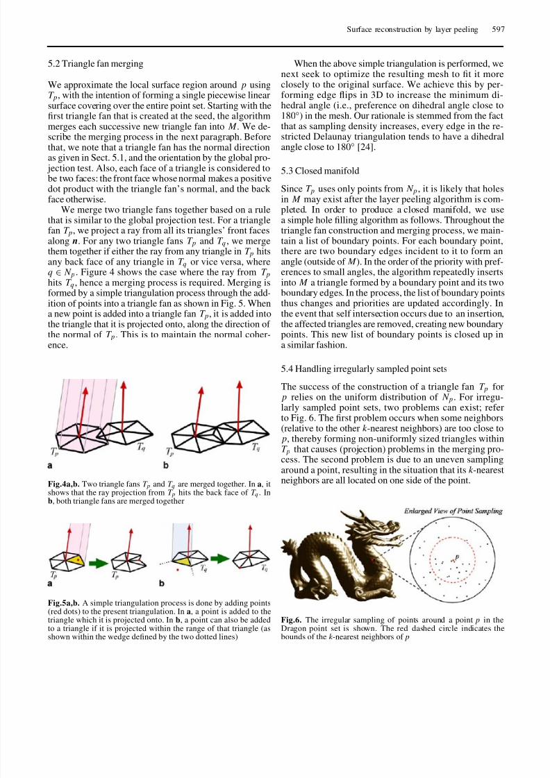
We merge two triangle fans together based on a rulethat is similar to the global projection test. For a trianglefan T p, we project a ray from all its triangles’ front facesalong n. For any two triangle fans T p and T q , we mergethem together if either the ray from any triangle in T p hitsany back face of any triangle in T q or vice versa, where

q ∈ N p. Figure 4 shows the case where the ray from T phits T q, hence a merging process is required. Merging isformed by a simple triangulation process through the add-ition of points into a triangle fan as shown in Fig. 5. Whena new point is added into a triangle fan T p, it is added intothe triangle that it is projected onto, along the direction of the normal of T p. This is to maintain the normal coher-ence.

Fig.4a,b. Two triangle fans T p and T q are merged together. In a, itshows that the ray projection from T p hits the back face of T q . Inb, both triangle fans are merged together

Fig.5a,b. A simple triangulation process is done by adding points(red dots) to the present triangulation. In a, a point is added to thetriangle which it is projected onto. In b, a point can also be addedto a triangle if it is projected within the range of that triangle (asshown within the wedge defined by the two dotted lines)

When the above simple triangulation is performed, wenext seek to optimize the resulting mesh to fit it moreclosely to the original surface. We achieve this by per-forming edge flips in 3D to increase the minimum di-hedral angle (i.e., preference on dihedral angle close to180◦) in the mesh. Our rationale is stemmed from the factthat as sampling density increases, every edge in the re-

stricted Delaunay triangulation tends to have a dihedralangle close to 180◦ [24].

5.3 Closed manifold

Since T p uses only points from N p, it is likely that holesin M may exist after the layer peeling algorithm is com-pleted. In order to produce a closed manifold, we usea simple hole filling algorithm as follows. Throughout thetriangle fan construction and merging process, we main-tain a list of boundary points. For each boundary point,there are two boundary edges incident to it to form anangle (outside of M ). In the order of the priority with pref-

erences to small angles, the algorithm repeatedly insertsinto M a triangle formed by a boundary point and its twoboundary edges. In the process, the list of boundary pointsthus changes and priorities are updated accordingly. Inthe event that self intersection occurs due to an insertion,the affected triangles are removed, creating new boundarypoints. This new list of boundary points is closed up ina similar fashion.

5.4 Handling irregularly sampled point sets

The success of the construction of a triangle fan T p forp relies on the uniform distribution of N p. For irregu-

larly sampled point sets, two problems can exist; referto Fig. 6. The first problem occurs when some neighbors(relative to the other k -nearest neighbors) are too close top, thereby forming non-uniformly sized triangles withinT p that causes (projection) problems in the merging pro-cess. The second problem is due to an uneven samplingaround a point, resulting in the situation that its k -nearestneighbors are all located on one side of the point.

Fig.6. The irregular sampling of points around a point p in theDragon point set is shown. The red dashed circle indicates thebounds of the k -nearest neighbors of p




To handle the first problem, we run a decimation pro-cess after the k -nearest neighbors are calculated for eachinput point. In this process, we scan through each point insome order (such as the input order) to remove its neigh-bors that are within 1

10of its estimated sampling distance.

Those surviving points at the end of the decimation pro-cess then have their k -nearest neighbors re-calculated, and

used to form the mesh M with the layer peeling algorithm.Thereafter, those points previously removed are mergedinto their nearest triangles in M . For the second problem,for each point p, we augment its k -nearest neighborhoodto include points which have p in their k -nearest neighbor-hood. This provides more choices for the construction of triangles for use in the triangle fan at p.

6 Analysis

In this section, we provide an analysis of our layer peel-ing algorithm. Section 6.1 provides an explanation thatthe proposed layer peeling algorithm can handle under-sampled point sets well. Furthermore, Sect. 6.2 shows thatunder optimal-sampling condition, the layer peeling algo-rithm is also a provable surface reconstruction algorithm.Section 6.3 discusses the computational time of our algo-rithm.

6.1 Under-sampled point sets

By the local convexity criterion used in the triangle fanconstruction, we avoid very effectively the problem of pforming a triangle fan with points in N p lying below the

surface containingp

. As for the other problem of pointslying above p but in N p, we explain in the next paragraphthat the layer peeling process can resolve it effectively,too.

For each triangle fan constructed, we test whether itpasses the global projection test before adding it to theheap for selection during the merging process. In thisway, the layer peeling algorithm can be visualized to beprogressing from the outer portion of the point set, andthen slowly moving inwards. As alluded by Theorem 1(Sect. 6.2), at any instance of the algorithm, there existsa point with no triangle fan constructed yet and is free of points lying above (or below, depending on the current it-eration) its local surface. By always choosing such a pointas the next candidate to construct and merge its trianglefan, we can avoid the problem of points within N p that lieabove the local surface around p.

6.2 Optimal-sampled point sets

The medial axis of the surface S is the closure of the setof points in R3 that has two or more closest points in S.The local feature size, f ( p), at a point p on S is the least

distance of p to the medial axis. The medial balls at pare defined as the balls that touch S tangentially at p andhave their centers on the medial axis. A point cloud P iscalled an ε-sample of S (where 0 < ε < 1), if every pointp ∈ S has a point in P at distance at most ε f ( p). For thepurpose of our proof, we require a stricter sampling con-dition, known as an (ε, δ)-sampling [15]. An ε-sample of

S is called an (ε, δ)-sample if it satisfies an additional con-dition:

∀p, q ∈ P : p−q ≥ δ f ( p) (1)

for ε2≤ δ < ε < 1.

For the remaining part of this section, we assume thepoint set P to be an (ε, δ)-sample. A method to obtain an(ε, δ)-sample from an ε-sample is provided in [18]. TheDelaunay triangulation of P restricted to S is the dualcomplex of the restricted Voronoi diagram of P. The re-stricted Voronoi diagram is the collection of all restrictedVoronoi cells, and the restricted Voronoi cell of a sample

point p ∈ P is the intersection of the Voronoi cell of pwith S. With these, we next provide the analysis of ourproposed algorithm.

We require two lemmas from [3, 19]. The first lemmabounds the maximum length of an edge in a restricted De-launay triangulation. The second lemma bounds the angleof the normals between two points that are sufficientlyclose.

Lemma 1. [19] For p, q ∈ P, if pq is an edge of the re-stricted Delaunay triangulation, then

p−q ≤2ε

1−εmin{ f ( p), f (q)}. (2)

Lemma 2. [3] For any two points p and q on S with p−q ≤ ρ min{ f ( p), f (q)}, for any ρ < 1

3, the angle between

the normal to S at p and at q is at most ρ

(1−3ρ).

Based on the above lemmas, we have the followingcorollary:

Corollary 1. For p, q ∈ P, if pq is an edge of the re-stricted Delaunay triangulation, then the angle betweenthe normal at p and at q is at most 38.1◦ for ε ≤ 0.1.

Proof. Combining Lemma 1 and Lemma 2, we let ρ be2ε

1−εto obtain ρ

1−3ρ=

2ε/(1−ε)1−6ε/(1−ε)

= 2ε1−7ε

. The maximum

angle difference of 38.1◦ is achieved with ε = 0.1.

In the following, we define the local region arounda point p as the space where all points within that regionis at most a distance of 2ε

1−εaway from p. For an (ε, δ)-

sample, [7] provides a formula to calculate the value of k ,such that N p contains all points within the local regionaround p. The next theorem shows that the layer peelingalgorithm does not prematurely terminate before a mani-fold is constructed. For the proof, it is sufficient to showthe existence of a seed to construct a triangle fan, though




our algorithm usually utilizes points from the boundary of M for the purpose.

Theorem 1. At any instance during the execution of thelayer peeling algorithm on a point set P, there always ex-ists a point p to construct a triangle fan T p to becomea part of M.

Proof. Let P ⊆ P where each point in P has no trianglefan constructed yet. We pick p ∈ P to be a vertex of theconvex hull of P. Next, we construct a triangle fan T p forp. Clearly, p with T p passes the global projection test; wenext show that T p satisfies the local convexity criterion andthe normal coherence condition.

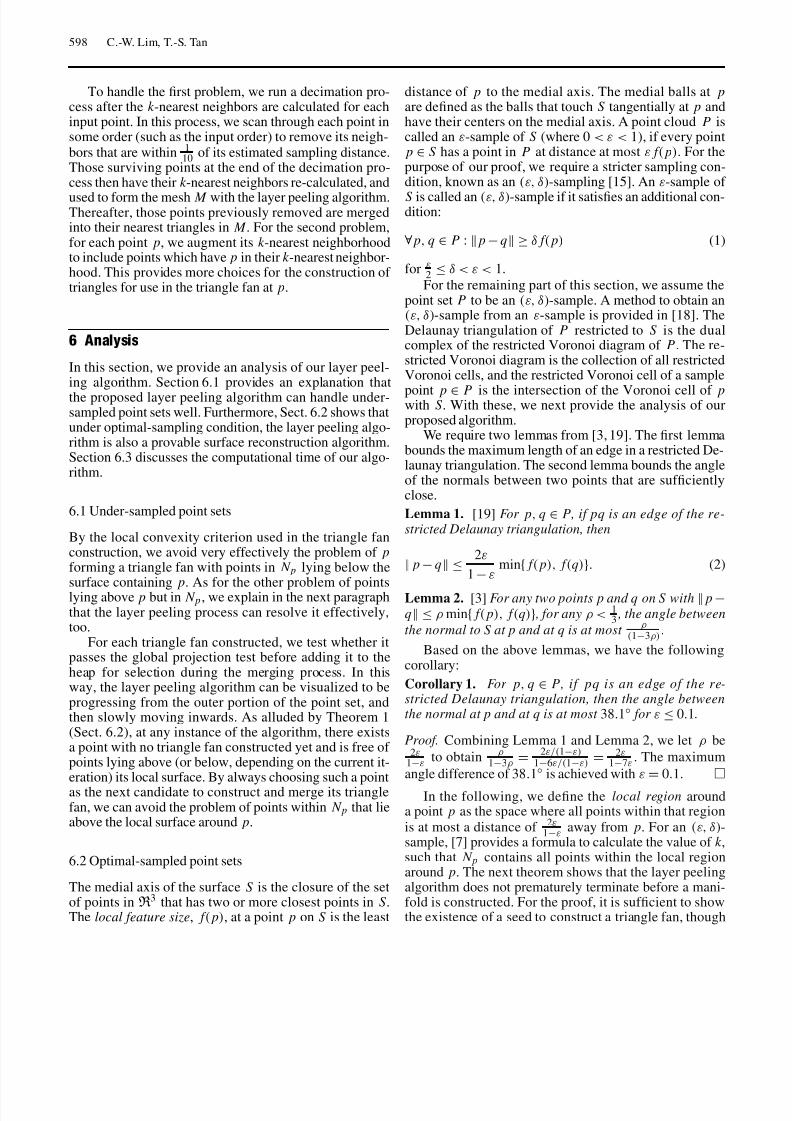
Refer to Fig. 7. For point p, the local region around p(shown in dashed red circle) is bounded by two balls of ra-dius f ( p). Now consider one of the balls, B. We tilt theball in any arbitrary direction while pivoting at point p un-til a point q is hit. Similar to [11], we now pivot the ballon the edge pq. By rotating the ball on the edge pq, ball Bcomes into contact with another point r (not shown in the

2D Fig. 7), forming a triangle pqr . Since the surface S is ε-sampled; therefore, a ball of radius ε f ( p) cannot penetrateS. Thus the maximum radius of the circumcircle of pqr can be at most ε f ( p). The maximum tilt of ball B happenswhen its surface intersects the other medial ball’s surfaceto form a circle of radius at most ε f ( p). (In the case whenε is 0.1, the maximum tilt is only 12◦ by a simple calcula-tion.) The maximum tilt of ball B is shown as B in Fig. 7.Furthermore, we note that p, q, and r exist in N p as q andr are of at most 2ε f ( p) distance away from p. To extractthe full T p, we continue to pivot the ball B on the edgepr and rotate away from q to extract the next triangle. Wecontinue in this fashion until T p is formed.

To prove that T p obeys the local convexity criterion,we consider each triangle of T p in turn. For each triangle,ball B is able to pivot on its three vertices. Since ball B isempty of points, the local convexity rule is easily seen toobey.

To show that normal coherence is obeyed by T p, weconsider the line pm, where m is the center of ball B.During the extraction of T p, the line pm traverses within

Fig. 7. A medial ball centered at m is pivoted at point p. The max-imum deviation of the line pm is pm

a cone-like space. After T p is formed, n lies within thiscone-like space. Since the tilt of pm never exceeds 90◦

(recall the maximum tilt for ε = 0.1 is only 12◦), normalcoherence condition is obeyed.

In the way we derive subsets of P (in step 3 of Fig. 3),Theorem 1 also holds for each subset. The next lemma

proves that the intersection of S

with the local regionaround any particular point p is a topological disk.

Lemma 3. Consider a point p ∈ P with n being the nor-mal to S at p, and a region S ⊆ S where S is the inter-section of S with the local region around p. Then thereexists an injective function to map S to a 2D plane witha normal of n for ε ≤ 0.1.

Proof. For any q ∈ S, we know that the maximum angledifference between the normals to S at p and q is 38.1◦

by corollary 1. Consider a line along the direction of n.It can intersect S at most once, since for intersection tooccur twice, the normal at some part of S needs to beat least more than 90◦ away from n. Thus we can definethe function µ as a linear projection from S using n asthe projection normal. It can easily be seen that µ is aninjective function, since no two points within S can beprojected to a single point.

From here, we can now begin to show how the outputfrom our layer peeling algorithm is homeomorphic to theoriginal surface where the point set is obtained.

Theorem 2. The piecewise linear surface constructed byour layer peeling algorithm is homeomorphic to the sur-face S for an (ε, δ)-sampled point set P where ε ≤ 0.1.

Proof. We aim to prove that, through a series of local op-

erations, we are able to transform the piecewise linearsurface constructed by our algorithm to the Delaunay tri-angulation of the input point set P restricted to S. Thetheorem, thus, follows as a Delaunay triangulation of P re-stricted to S with ε ≤ 0.1 is homeomorphic to the originalsurface S as proved in [4].

First, we show that the restricted Delaunay triangula-tion within the local region of p can be projected to a2D plane. By Lemma 3, the local region around p can beprojected into a 2D plane smoothly. Since those restrictedVoronoi cells are on the surface within the local region of p, they can also be projected similarly. Thus, it followsthat those dual restricted Delaunay edges can be projected

as well.Next, we consider the piecewise linear surface pro-duced by our algorithm. It cannot be projected straight-forwardly to a 2D plane as in the restricted Delaunaytriangulation case. This is because, with a small chance,the merging of a triangle fan at p to the mesh M canproduce a triangle incident to p whose normal can be al-most orthogonal to n, where n is the normal to S at p.Such a triangulation occurs because of badly shaped sliver,for example a splinter or spike sliver, as classified in [13],




where edge flipping may not be able to remove. Neverthe-less, we can transform the triangulation around the localregion of p to one that minimizes the maximum slopevia the edge insertion technique [10]. Such a triangulationdoes not have badly shaped triangles as the local region tobe constructed is known to obey Lemma 3. With this, wecan now project the triangulation around the local region

of p to a 2D plane.With both the restricted Delaunay triangulation and our

triangulation around the local region of p projected to a2D plane, we can use edge flip operations in 2D to trans-form from one to the other. This is because in 2D fora fixed set of points, any triangulation is transformable toanother one through a series of edge flips. Thus, we cantransform our piecewise linear surface to the restrictedDelaunay triangulation. This completes our series of oper-ations and the proof.

6.3 Computational time

In general, our algorithm is mostly local. However, thereare two portions of the algorithm with non-linear timecomplexity. The first is the computation of the k -nearestneighbors [8, 26] while the other is the global projectiontest. For both cases, the data structures consist of spatialtree decomposition approaches. Both require O(n log n)time to construct, and O(log n) time to process for eachpoint where n is the number of input points. For the for-mer, we only construct it once at the start of the algo-rithm and the actual timing taken by this process is in-significant when compared with that by the rest of thealgorithm. For the latter case, the construction time is

similarly insignificant, but the global projection test canbe expensive as each point may perform the test manytimes during its triangle fan construction. However, wenote that for each subsequent layer, the size of the oc-tree gets progressively smaller as the point set is splitinto subsets. Hence, the influence of the non-linear timecomplexity portions of the algorithm is not so evident asshown in our experimental results reported in the next sec-tion.

7 Experimental results

We have implemented our algorithm on a Pentium IV3.0GHz, 4GB DDR2 RAM and nVidia GeForce 6600with 256MB DDR3 video memory. For purposes of comparison, we downloaded the commonly used Tight-Cocone software [16] to run on the same machine asa benchmarking algorithm. For our implementation, wetake 16 to be the value of k . Although the upper boundstated in [7] is 32, we found that for our experiments16 is sufficient. For a comprehensive comparison, weuse nine real point sets (indicated in Fig. 12) available

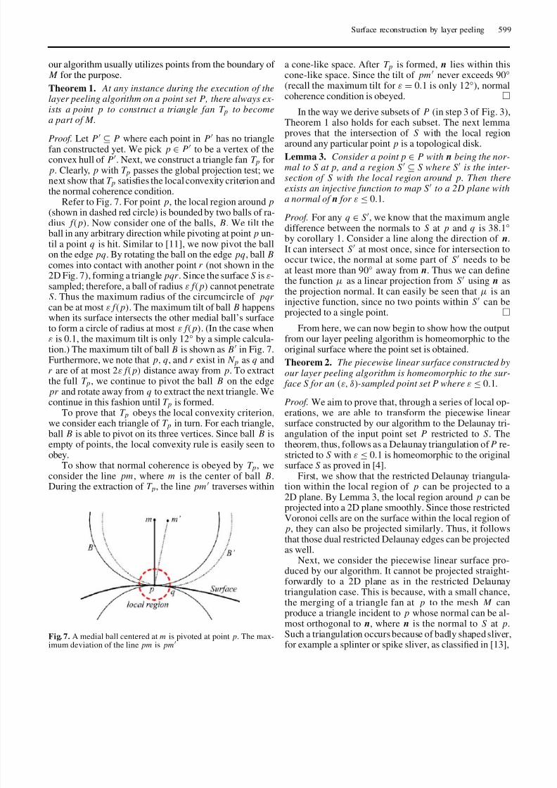
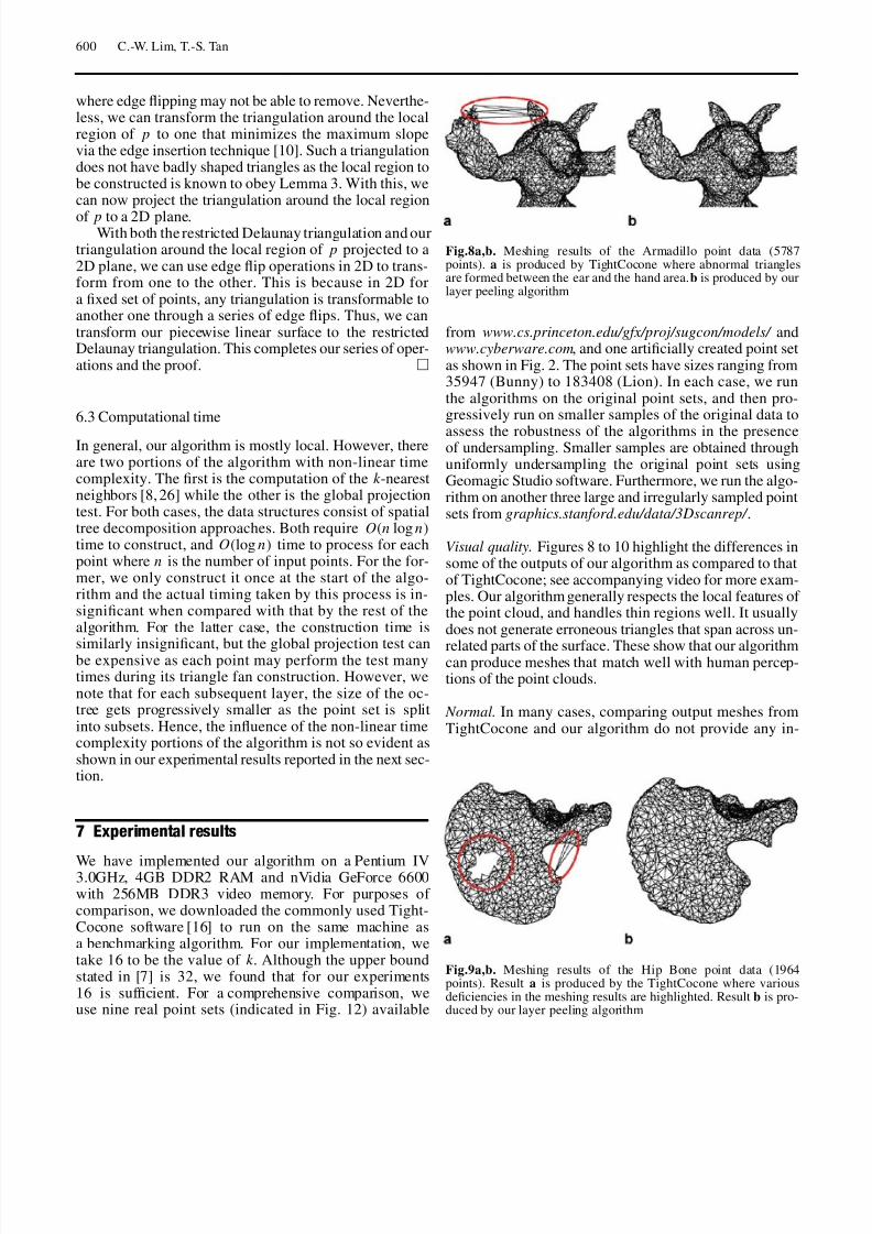
Fig.8a,b. Meshing results of the Armadillo point data (5787points). a is produced by TightCocone where abnormal trianglesare formed between the ear and the hand area. b is produced by ourlayer peeling algorithm

from www.cs.princeton.edu/gfx/proj/sugcon/models/ andwww.cyberware.com, and one artificially created point setas shown in Fig. 2. The point sets have sizes ranging from35947 (Bunny) to 183408 (Lion). In each case, we runthe algorithms on the original point sets, and then pro-gressively run on smaller samples of the original data to

assess the robustness of the algorithms in the presenceof undersampling. Smaller samples are obtained throughuniformly undersampling the original point sets usingGeomagic Studio software. Furthermore, we run the algo-rithm on another three large and irregularly sampled pointsets from graphics.stanford.edu/data/3Dscanrep/ .

Visual quality. Figures 8 to 10 highlight the differences insome of the outputs of our algorithm as compared to thatof TightCocone; see accompanying video for more exam-ples. Our algorithm generally respects the local features of the point cloud, and handles thin regions well. It usuallydoes not generate erroneous triangles that span across un-

related parts of the surface. These show that our algorithmcan produce meshes that match well with human percep-tions of the point clouds.

Normal. In many cases, comparing output meshes fromTightCocone and our algorithm do not provide any in-

Fig.9a,b. Meshing results of the Hip Bone point data (1964points). Result a is produced by the TightCocone where variousdeficiencies in the meshing results are highlighted. Result b is pro-duced by our layer peeling algorithm




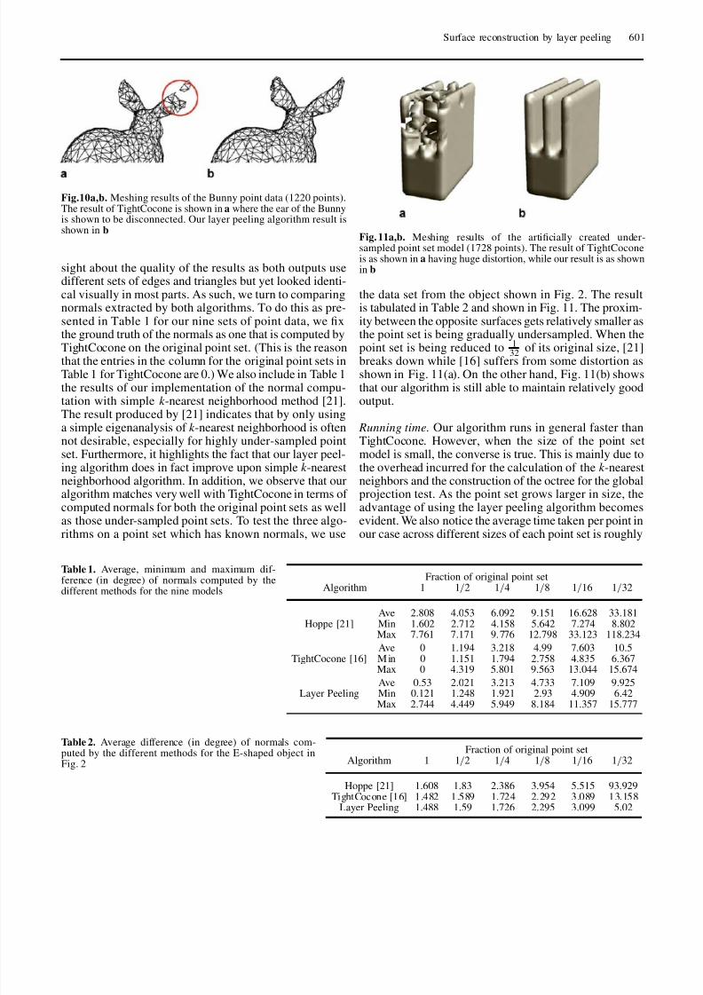
Fig.10a,b. Meshing results of the Bunny point data (1220 points).The result of TightCocone is shown in a where the ear of the Bunnyis shown to be disconnected. Our layer peeling algorithm result isshown in b

sight about the quality of the results as both outputs usedifferent sets of edges and triangles but yet looked identi-cal visually in most parts. As such, we turn to comparingnormals extracted by both algorithms. To do this as pre-sented in Table 1 for our nine sets of point data, we fixthe ground truth of the normals as one that is computed by

TightCocone on the original point set. (This is the reasonthat the entries in the column for the original point sets inTable 1 for TightCocone are 0.) We also include in Table 1the results of our implementation of the normal compu-tation with simple k -nearest neighborhood method [21].The result produced by [21] indicates that by only usinga simple eigenanalysis of k -nearest neighborhood is oftennot desirable, especially for highly under-sampled pointset. Furthermore, it highlights the fact that our layer peel-ing algorithm does in fact improve upon simple k -nearestneighborhood algorithm. In addition, we observe that ouralgorithm matches very well with TightCocone in terms of computed normals for both the original point sets as well

as those under-sampled point sets. To test the three algo-rithms on a point set which has known normals, we use

Fraction of original point setAlgorithm 1 1/2 1/4 1/8 1/16 1/32

Ave 2.808 4.053 6.092 9.151 16.628 33.181Hoppe [21] Min 1.602 2.712 4.158 5.642 7.274 8.802

Max 7.761 7.171 9.776 12.798 33.123 118.234

Ave 0 1.194 3.218 4.99 7.603 10.5TightCocone [16] M in 0 1.151 1.794 2.758 4.835 6.367

Max 0 4.319 5.801 9.563 13.044 15.674

Ave 0.53 2.021 3.213 4.733 7.109 9.925

Layer Peeling Min 0.121 1.248 1.921 2.93 4.909 6.42Max 2.744 4.449 5.949 8.184 11.357 15.777

Table 1. Average, minimum and maximum dif-ference (in degree) of normals computed by thedifferent methods for the nine models

Fraction of original point setAlgorithm 1 1/2 1/4 1/8 1/16 1/32

Hoppe [21] 1.608 1.83 2.386 3.954 5.515 93.929TightCocone [16] 1.482 1.589 1.724 2.292 3.089 13.158

Layer Peeling 1.488 1.59 1.726 2.295 3.099 5.02

Table 2. Average difference (in degree) of normals com-puted by the different methods for the E-shaped object inFig. 2

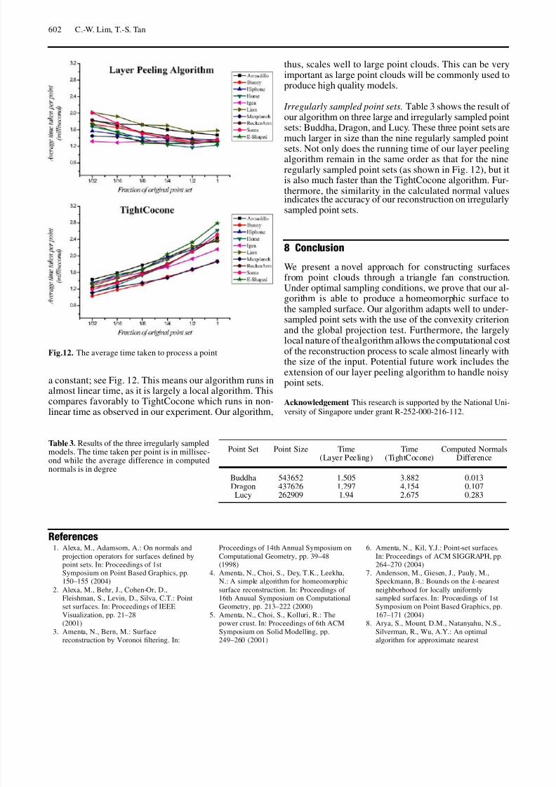
Fig. 11a,b. Meshing results of the artificially created under-sampled point set model (1728 points). The result of TightCoconeis as shown in a having huge distortion, while our result is as shownin b

the data set from the object shown in Fig. 2. The resultis tabulated in Table 2 and shown in Fig. 11. The proxim-ity between the opposite surfaces gets relatively smaller asthe point set is being gradually undersampled. When the

point set is being reduced to1

32 of its original size, [21]breaks down while [16] suffers from some distortion asshown in Fig. 11(a). On the other hand, Fig. 11(b) showsthat our algorithm is still able to maintain relatively goodoutput.

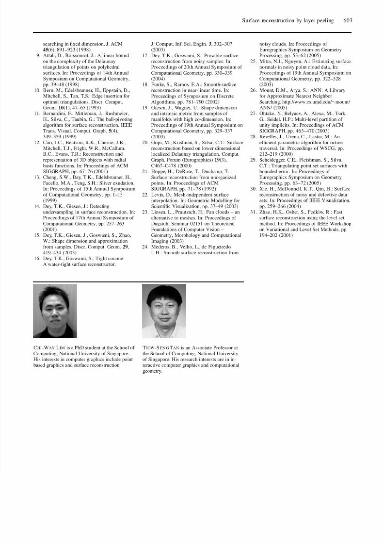
Running time. Our algorithm runs in general faster thanTightCocone. However, when the size of the point setmodel is small, the converse is true. This is mainly due tothe overhead incurred for the calculation of the k -nearestneighbors and the construction of the octree for the globalprojection test. As the point set grows larger in size, theadvantage of using the layer peeling algorithm becomes

evident. We also notice the average time taken per point inour case across different sizes of each point set is roughly




Fig.12. The average time taken to process a point

a constant; see Fig. 12. This means our algorithm runs inalmost linear time, as it is largely a local algorithm. Thiscompares favorably to TightCocone which runs in non-

linear time as observed in our experiment. Our algorithm,

Point Set Point Size Time Time Computed Normals(Layer Peeling) (TightCocone) Difference

Buddha 543652 1.505 3.882 0.013Dragon 437626 1.297 4.154 0.107

Lucy 262909 1.94 2.675 0.283

Table 3. Results of the three irregularly sampledmodels. The time taken per point is in millisec-ond while the average difference in computednormals is in degree

thus, scales well to large point clouds. This can be veryimportant as large point clouds will be commonly used toproduce high quality models.

Irregularly sampled point sets. Table 3 shows the result of our algorithm on three large and irregularly sampled pointsets: Buddha, Dragon, and Lucy. These three point sets are

much larger in size than the nine regularly sampled pointsets. Not only does the running time of our layer peelingalgorithm remain in the same order as that for the nineregularly sampled point sets (as shown in Fig. 12), but itis also much faster than the TightCocone algorithm. Fur-thermore, the similarity in the calculated normal valuesindicates the accuracy of our reconstruction on irregularlysampled point sets.

8 Conclusion

We present a novel approach for constructing surfaces

from point clouds through a triangle fan construction.Under optimal sampling conditions, we prove that our al-gorithm is able to produce a homeomorphic surface tothe sampled surface. Our algorithm adapts well to under-sampled point sets with the use of the convexity criterionand the global projection test. Furthermore, the largelylocal nature of the algorithm allows the computational costof the reconstruction process to scale almost linearly withthe size of the input. Potential future work includes theextension of our layer peeling algorithm to handle noisypoint sets.

Acknowledgement This research is supported by the National Uni-

versity of Singapore under grant R-252-000-216-112.

References

1. Alexa, M., Adamsom, A.: On normals andprojection operators for surfaces defined bypoint sets. In: Proceedings of 1stSymposium on Point Based Graphics, pp.150–155 (2004)

2. Alexa, M., Behr, J., Cohen-Or, D.,Fleishman, S., Levin, D., Silva, C.T.: Pointset surfaces. In: Proceedings of IEEE

Visualization, pp. 21–28(2001)

3. Amenta, N., Bern, M.: Surfacereconstruction by Voronoi filtering. In:

Proceedings of 14th Annual Symposium onComputational Geometry, pp. 39–48(1998)

4. Amenta, N., Choi, S., Dey, T.K., Leekha,N.: A simple algorithm for homeomorphic

surface reconstruction. In: Proceedings of 16th Anuual Symposium on ComputationalGeometry, pp. 213–222 (2000)

5. Amenta, N., Choi, S., Kolluri, R.: Thepower crust. In: Proceedings of 6th ACM

Symposium on Solid Modelling, pp.249–260 (2001)

6. Amenta, N., Kil, Y.J.: Point-set surfaces.In: Proceedings of ACM SIGGRAPH, pp.264–270 (2004)

7. Andersson, M., Giesen, J., Pauly, M.,Speckmann, B.: Bounds on the k -nearest

neighborhood for locally uniformlysampled surfaces. In: Proceedings of 1stSymposium on Point Based Graphics, pp.

167–171 (2004)8. Arya, S., Mount, D.M., Natanyahu, N.S.,

Silverman, R., Wu, A.Y.: An optimalalgorithm for approximate nearest




searching in fixed dimension. J. ACM45(6), 891–923 (1998)

9. Attali, D., Boissonnat, J.: A linear bound

on the complexity of the Delaunaytriangulation of points on polyhedral

surfaces. In: Proceedings of 14th Annual

Symposium on Computational Geometry,pp. 39–48 (1998)

10. Bern, M., Edelsbrunner, H., Eppstein, D.,

Mitchell, S., Tan, T.S.: Edge insertion foroptimal triangulations. Discr. Comput.Geom. 10(1), 47–65 (1993)

11. Bernardini, F., Mittleman, J., Rushmeier,

H., Silva, C., Taubin, G.: The ball-pivotingalgorithm for surface reconstruction. IEEE

Trans. Visual. Comput. Graph. 5(4),349–359 (1999)

12. Carr, J.C., Beatson, R.K., Cherrie, J.B.,Mitchell, T.J., Fright, W.R., McCallum,B.C., Evans, T.R.: Reconstruction and

representation of 3D objects with radial

basis functions. In: Proceedings of ACMSIGGRAPH, pp. 67–76 (2001)

13. Cheng, S.W., Dey, T.K., Edelsbrunner, H.,

Facello, M.A., Teng, S.H.: Sliver exudation.

In: Proceedings of 15th Annual Symposiumof Computational Geometry, pp. 1–13(1999)

14. Dey, T.K., Giesen, J.: Detectingundersampling in surface reconstruction. In:Proceedings of 17th Annual Symposium of

Computational Geometry, pp. 257–263(2001)

15. Dey, T.K., Giesen, J., Goswami, S., Zhao,W.: Shape dimension and approximation

from samples. Discr. Comput. Geom. 29,

419–434 (2003)16. Dey, T.K., Goswami, S.: Tight cocone:

A water-tight surface reconstructor.

J. Comput. Inf. Sci. Engin. 3, 302–307(2003)

17. Dey, T.K., Goswami, S.: Provable surfacereconstruction from noisy samples. In:Proceedings of 20th Annual Symposium of


18. Funke, S., Ramos, E.A.: Smooth-surfacereconstruction in near-linear time. In:

Proceedings of Symposium on DiscreteAlgorithms, pp. 781–790 (2002)

19. Giesen, J., Wagner, U.: Shape dimension

and intrinsic metric from samples of manifolds with high co-dimension. In:Proceedings of 19th Annual Symposium on

Computational Geometry, pp. 329–337

(2003)20. Gopi, M., Krishnan, S., Silva, C.T.: Surface

reconstruction based on lower dimensional

localized Delaunay triangulation. Comput.Graph. Forum (Eurographics) 19(3),

C467–C478 (2000)21. Hoppe, H., DeRose, T., Duchamp, T.:

Surface reconstruction from unorganizedpoints. In: Proceedings of ACM

SIGGRAPH, pp. 71–78 (1992)22. Levin, D.: Mesh-independent surfaceinterpolation. In: Geometric Modelling forScientific Visualization, pp. 37–49 (2003)

23. Linsen, L., Prautzsch, H.: Fan clouds – an

alternative to meshes. In: Proceedings of

Dagstuhl Seminar 02151 on TheoreticalFoundations of Computer Vision –Geometry, Morphology and Computational

Imaging (2003)24. Mederos, B., Velho, L., de Figueiredo,

L.H.: Smooth surface reconstruction from

noisy clouds. In: Proceedings of Eurographics Symposium on GeometryProcessing, pp. 53–62 (2005)

25. Mitra, N.J., Nguyen, A.: Estimating surfacenormals in noisy point cloud data. In:

Proceedings of 19th Annual Symposium on


26. Mount, D.M., Arya, S.: ANN: A Library

for Approximate Nearest NeighborSearching. http://www.cs.umd.edu/ ∼mount/ ANN/ (2005)

27. Ohtake, Y., Belyaev, A., Alexa, M., Turk,

G., Seidel, H.P.: Multi-level partition of unity implicits. In: Proceedings of ACM

SIGGRAPH, pp. 463–470 (2003)28. Revelles, J., Urena, C., Lastra, M.: An

efficient parametric algorithm for octreetraversal. In: Proceedings of WSCG, pp.212–219 (2000)

29. Scheidegger, C.E., Fleishman, S., Silva,

C.T.: Triangulating point set surfaces withbounded error. In: Proceedings of Eurographics Symposium on Geometry

Processing, pp. 63–72 (2005)

30. Xie, H., McDonnell, K.T., Qin, H.: Surfacereconstruction of noisy and defective datasets. In: Proceedings of IEEE Visualization,

pp. 259–266 (2004)31. Zhao, H.K., Osher, S., Fedkiw, R.: Fast

surface reconstruction using the level set

method. In: Proceedings of IEEE Workshopon Variational and Level Set Methods, pp.194–202 (2001)

CHI -WAN LIM is a PhD student at the School of

Computing, National University of Singapore.His interests in computer graphics include point

based graphics and surface reconstruction.

TIOW -S EN G TAN is an Associate Professor at

the School of Computing, National Universityof Singapore. His research interests are in in-

teractive computer graphics and computational

geometry.

Documents

Surface Reconstruction by layer peeling