Embed Size (px)
Citation preview
SWAMP Bioassessment
Procedures 2016
Standard Operating Procedures (SOP) for the Collection of Field Data for Bioassessments of California Wadeable Streams: Benthic Macroinvertebrates, Algae, and Physical Habitat
March 2016 v2 (unformatted)
Peter R. Ode1, A. Elizabeth Fetscher2 and Lilian B. Busse3
1 Aquatic Bioassessment Laboratory/Water Pollution Control Laboratory California Department of Fish and Wildlife 2005 Nimbus Road Rancho Cordova, CA 95670 2 San Diego Regional Water Quality Control Board 2375 Northside Drive, Suite 100 San Diego, CA 92108-2700 (Work carried out at the Southern California Coastal Water Research Project) 3 San Diego Regional Water Quality Control Board 2375 Northside Drive, Suite 100 San Diego, CA 92108-2700 (Current address: German Federal Environment Agency, Woerlitzer Platz 1, 06844 Dessau, Germany)
2
TABLE OF CONTENTS
Table of Contents ............................................................................................................................ 2 Acknowledgements .......................................................................................................................... 4 Abbreviations and Acronyms .......................................................................................................... 6 1. Introduction................................................................................................................................. 7
1.1 Previous SOPs ....................................................................................................................... 7 1.2 Sampling Overview ............................................................................................................ 10 1.3 Scope and Applicability ...................................................................................................... 11 1.4 Diagnosing Recent Scour .................................................................................................... 12 1.5 Training ............................................................................................................................... 16 1.6 Permitting ............................................................................................................................ 16 1.7 Avoiding the Transfer of Invasive Species and Pathogens Amongst Sites ........................ 17 1.8 SWAMP Requirements ....................................................................................................... 17 1.9 Supplemental Guidance ...................................................................................................... 18
2. Reach Delineation and scoring noteable filed conditions ........................................................ 18 3. Water Chemistry Sampling ....................................................................................................... 22 4. Biotic Community Sampling ..................................................................................................... 24
4.1 The Reachwide Benthos (RWB) Method for Biotic Sample Collection ............................ 24 4.2 General Considerations for Sampling BMIs ....................................................................... 25 4.3 Module A: RWB Sampling Procedure for BMIs ................................................................ 25 4.4 General Considerations for Sampling Benthic Algae ......................................................... 27 4.5 Module B: RWB Sampling Procedure for Benthic Algae – Quantitative Samples ............ 30
4.5.1 Collecting from Cobbles, Large Gravel, and Wood Using the Rubber Delimiter ....... 31 4.5.2 Collecting from Sediment ............................................................................................ 32 4.5.3 Collecting a Mass of Macroalgae Using the ABS delimiter ........................................ 33 4.5.4 Collecting from Macrophytes ...................................................................................... 33 4.5.5 Collecting from Hard, Submerged, Anchored Substrates: Concrete, Bedrock, and Boulders ................................................................................................................................ 33 4.5.6 Collecting from Other Substrate Types ....................................................................... 34
4.6 Module B (continued): Procedure for Collecting and Storing Qualitative Soft Algae Samples ..................................................................................................................................... 35
5. Biotic Sample Processing ......................................................................................................... 37 5.1 Module A (continued): Processing Benthic Macroinvertebrate Samples ........................... 37 5.2 Module B (continued): Processing Quantitative Benthic Algal Taxonomy and Biomass Samples ..................................................................................................................................... 38
6. Physical Habitat Transect-Based Measurements ..................................................................... 51 6.1 Module C: Wetted Width and Bankfull Dimensions .......................................................... 51 6.2 Module D: Substrate Size, Depth, and Coarse Particulate Organic Matter (CPOM) ......... 52 6.3 Module E: Cobble Embeddedness ...................................................................................... 55 6.4 Module F: Algal and Macrophyte Cover ............................................................................ 56 6.5 Module G: Bank Stability ................................................................................................... 58 6.6 Module H: Human Influence .............................................................................................. 58 6.7 Module I: Riparian Vegetation ........................................................................................... 60 6.8 Module J: Instream Habitat Complexity ............................................................................. 62 6.9 Module K: Stream Shading (Densiometer Readings) ......................................................... 63

3
6.10 Module L: Slope and Sinuosity......................................................................................... 65 6.10.1 Slope - autolevel method ........................................................................................... 66 6.10.2 Slope - clinometer method ......................................................................................... 67 6.10.3 Sinuosity .................................................................................................................... 68
6.11 Module M: Photographs ................................................................................................... 68 7. Physical Habitat Inter-Transect-Based Measurements ............................................................ 69
7.1 Module C (part two): Inter-transect Wetted Width............................................................. 69 7.2 Modules D, E, and F (part two): Substrate Measurements, Depth, CPOM, and Algal/Macrophyte Percent Cover ............................................................................................. 69 7.3 Module N: Flow Habitats.................................................................................................... 69
8. Physical Habitat Reach-Based Measurements ......................................................................... 71 8.1 Module O: Stream Discharge .............................................................................................. 71
8.1.1 Velocity Area Method.................................................................................................. 71 8.1.2 Neutrally Buoyant Object Method ............................................................................... 73
8.2 Module P: Post-Sampling Observations: Qualitative Reach Measures .............................. 74 8. Optional Supplemental Measures ............................................................................................. 75 9. References ................................................................................................................................. 76 10. Glossary .................................................................................................................................. 79
4
ACKNOWLEDGEMENTS
This Standard Operating Procedures (SOP) manual represents the contributions of a wide range of researchers and field crews (see below). The benthic macroinvertebrate and algae specimen and physical habitat data collection methodology presented represent modifications of the U.S. Environmental Protection Agency’s (EPA) Environmental Monitoring and Assessment Program (EMAP) multihabitat sampling protocol (Peck et al. 2006). Point-intercept estimation of macroalgal cover has been adapted from the U.S. Geological Survey’s (USGS) National Water Quality Assessment pilot procedures (J. Berkman, pers comm.), and assessment of microalgal thickness has been adapted from Stevenson and Rollins (2006). This protocol was developed and greatly improved as the result of contributions from a large group of people who participated in internal reviews, provided feedback during field testing, and read various iterations of this document. We thank especially the following for their contributions: Karissa Anderson (San Francisco Regional Water Quality Control Board) Dean Blinn (Northern Arizona University) Matt Cover (California State University, Stanislaus) Erick Burres (Clean Water Team, State Water Resources Control Board) Will Hagan (SWAMP Quality Assurance Team) Mary Hamilton (Central Coast Regional Water Quality Control Board) Julie Berkman (US Geological Survey) James Harrington (Aquatic Bioassessment Laboratory, California Department of Fish and
Wildlife) Charles Hawkins (Utah State University) David Herbst (Sierra Nevada Aquatic Research Laboratory, University of California Santa
Barbara) Robert Hughes (Dynamac) Gary Ichikawa (Marine Pollution Studies Laboratory, California Department of Fish and
Wildlife) Bill Isham (Weston Solutions) Scott Johnson (Aquatic Bioassay & Consulting Laboratories) Phil Kaufmann (US Environmental Protection Agency) Revital Katznelson Patrick Kociolek (University of Colorado Boulder) Berengere Laslandes (University of Colorado Boulder) Carrieann Lopez (North Coast Regional Water Quality Control Board) Marc Los Huertos (California State University Monterey Bay) Kevin Lunde (San Francisco Bay Regional Water Quality Control Board Nathan Mack (Aquatic Bioassessment Laboratory, California Department of Fish and Wildlife) Toni Marshall (Information Management and Quality Assurance Center, State Water Resources
Control Board) Raphael Mazor (Southern California Coastal Water Research Project and Aquatic Bioassessment
Laboratory, California Department of Fish and Wildlife)
5
Shawn McBride (Aquatic Bioassessment Laboratory, California Department of Fish and Wildlife)
Sean Mundell (Marine Pollution Studies Laboratory, California Department of Fish and Wildlife)
Damon Owen (Weston Solutions) Karin Patrick (Aquatic Bioassay & Consulting Laboratories) David Peck (US Environmental Protection Agency) Marc Petta (Information Management and Quality Assurance Center, State Water Resources
Control Board) Craig Pernot (Aquatic Bioassay & Consulting Laboratories) Daniel Pickard (Aquatic Bioassessment Laboratory, California Department of Fish and Wildlife) Doug Post (Aquatic Bioassessment Laboratory, California Department of Fish and Wildlife) Andrew Rehn (Aquatic Bioassessment Laboratory, California Department of Fish and Wildlife) Robert Holmes (California Department of Fish and Wildlife) Scott Rollins (Spokane Falls Community College) Jay Rowan (California Department of Fish and Wildlife) John Sandberg (Aquatic Bioassessment Laboratory, California Department of Fish and Wildlife) Robert Sheath (California State University San Marcos) Glenn Sibbald (Aquatic Bioassessment Laboratory, California Department of Fish and Wildlife) Marco Sigala ( Marine Pollution Studies Laboratory, Moss Landing Marine Laboratories) Joseph Slusark (Aquatic Bioassessment Laboratory, California Department of Fish and Wildlife) Rosalina Stancheva (California State University San Marcos) Thomas Suk (Lahontan Regional Water Quality Control Board) Martha Sutula (Southern California Coastal Water Research Project) Karen Taberski (San Francisco Regional Water Quality Control Board) Evan Thomas (University of Colorado Boulder) Jonathan Warmerdam (North Coast Regional Water Quality Control Board) David Williams (San Francisco Bay Regional Water Quality Control Board) Melinda Woodard (Marine Pollution Studies Laboratory, Moss Landing Marine Laboratories) Jennifer York (Aquatic Bioassessment Laboratory, California Department of Fish and Wildlife) Yangdong Pan (Portland State University)
Citation for this document: Ode, P.R., A.E., Fetscher, and L.B. Busse. 2016. Standard Operating Procedures for the Collection of Field Data for Bioassessments of California Wadeable Streams: Benthic Macroinvertebrates, Algae, and Physical Habitat. California State Water Resources Control Board Surface Water Ambient Monitoring Program (SWAMP) Bioassessment SOP 004
6
ABBREVIATIONS AND ACRONYMS
AFDM Ash-Free Dry Mass BMI Benthic Macroinvertebrate chl a Chlorophyll a CPOM Coarse Particulate Organic Matter CSBP California Stream Bioassessment Procedure DI Deionized water DO Dissolved Oxygen DFW (California) Department of Fish and Wildlife EMAP Environmental Monitoring and Assessment Program (of the U.S. EPA) EPA Environmental Protection Agency (of the United States) GPS Global Positioning System IBI Index of Biotic Integrity LRBS Log Relative Bed Stability MCM Margin-Center-Margin NAD North American Datum NBO Neutrally Buoyant Object NNE Nutrient Numeric Endpoints NRSA National Rivers and Streams Assessment (of the U.S. EPA) PHab Physical Habitat QA Quality Assurance QAPrP Quality Assurance Program Plan (of SWAMP) RBP Rapid Bioassessment Procedures RWB Reachwide Benthos SOP Standard Operating Procedures SCCWRP Southern California Coastal Water Research Project SWAMP Surface Water Ambient Monitoring Program (of the California State Water
Resources Control Board) TRC Targeted Riffle Composite VAM Velocity-Area Method (for determining stream discharge)
7
1. INTRODUCTION
This document describes the Standard Operating Procedures (SOP) for bioassessment of wadeable streams for the California State Water Resources Control Board’s Surface Water Ambient Monitoring Program (SWAM). These procedures are recognized by the US Environmental Protection Agency (EPA) as California’s standard bioassessment procedures and are designed to support general assessment of the ecological condition of wadeable streams and rivers based on the composition of the benthic macroinvertebrate and benthic algal assemblages. The procedures also produce standardized measurements of instream and riparian habitat and ambient water chemistry to support interpretation of the biological data. Instructions are provided for collection of the following: • samples for taxonomic analysis of benthic macroinvertebrate (BMI) assemblages • samples for taxonomic analysis of benthic algal assemblages (diatoms & non-diatom (soft)
algae (including cyanobacteria)) • samples for determination of biomass based on benthic chlorophyll a and benthic ash-free dry
mass (AFDM) • stream physical habitat (PHab) data • water chemistry samples 1.1 Previous SOPs This document represents a consolidation of two closely related previous SOPs, and supersedes them: • Ode (2007), which focused on stream BMI sampling and associated PHab data collection and
replaced previous bioassessment protocols referred to as the California Stream Bioassessment Procedure (CSBP, Harrington 1995, 1999, 2002), and
• Fetscher et al. (2009), which focused on stream benthic algae and biomass sampling, and associated PHab data collection.
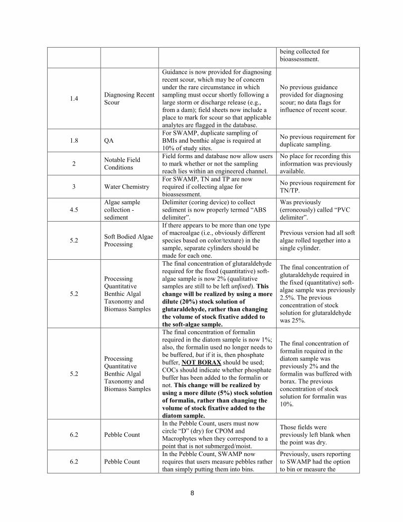
Most of the methods described here are close adaptations of those developed by the EPA’s Environmental Monitoring and Assessment Program (EMAP) and currently used by the EPA’s National Rivers and Streams Assessment (NRSA) surveys. Table 1 provides a summary of the major changes to field procedures since the previous SOPs. Summary of Changes Table 1 Summary of Changes
Section Category Current Protocol Previous Versions (Ode 2007 & Fetscher et al.
2009)
General General
For SWAMP, the "Full" set of PHab modules must be carried out, even if just collecting algae (and not BMIs) as the biotic assemblage.
Previously, modules such as Riparian Vegetation and Instream Habitat Complexity were not required if only algae were
8
being collected for bioassessment.
1.4 Diagnosing Recent Scour
Guidance is now provided for diagnosing recent scour, which may be of concern under the rare circumstance in which sampling must occur shortly following a large storm or discharge release (e.g., from a dam); field sheets now include a place to mark for scour so that applicable analytes are flagged in the database.
No previous guidance provided for diagnosing scour; no data flags for influence of recent scour.
1.8 QA For SWAMP, duplicate sampling of BMIs and benthic algae is required at 10% of study sites.
No previous requirement for duplicate sampling.
2 Notable Field Conditions
Field forms and database now allow users to mark whether or not the sampling reach lies within an engineered channel.
No place for recording this information was previously available.
3 Water Chemistry For SWAMP, TN and TP are now required if collecting algae for bioassessment.
No previous requirement for TN/TP.
4.5 Algae sample collection - sediment
Delimiter (coring device) to collect sediment is now properly termed “ABS delimiter”.
Was previously (erroneously) called “PVC delimiter”.
5.2 Soft Bodied Algae Processing
If there appears to be more than one type of macroalgae (i.e., obviously different species based on color/texture) in the sample, separate cylinders should be made for each one.
Previous version had all soft algae rolled together into a single cylinder.
5.2
Processing Quantitative Benthic Algal Taxonomy and Biomass Samples
The final concentration of glutaraldehyde required for the fixed (quantitative) soft-algae sample is now 2% (qualitative samples are still to be left unfixed). This change will be realized by using a more dilute (20%) stock solution of glutaraldehyde, rather than changing the volume of stock fixative added to the soft-algae sample.
The final concentration of glutaraldehyde required in the fixed (quantitative) soft-algae sample was previously 2.5%. The previous concentration of stock solution for glutaraldehyde was 25%.
5.2
Processing Quantitative Benthic Algal Taxonomy and Biomass Samples
The final concentration of formalin required in the diatom sample is now 1%; also, the formalin used no longer needs to be buffered, but if it is, then phosphate buffer, NOT BORAX should be used; COCs should indicate whether phosphate buffer has been added to the formalin or not. This change will be realized by using a more dilute (5%) stock solution of formalin, rather than changing the volume of stock fixative added to the diatom sample.
The final concentration of formalin required in the diatom sample was previously 2% and the formalin was buffered with borax. The previous concentration of stock solution for formalin was 10%.
6.2 Pebble Count
In the Pebble Count, users must now circle “D” (dry) for CPOM and Macrophytes when they correspond to a point that is not submerged/moist.
Those fields were previously left blank when the point was dry.
6.2 Pebble Count In the Pebble Count, SWAMP now requires that users measure pebbles rather than simply putting them into bins.
Previously, users reporting to SWAMP had the option to bin or measure the
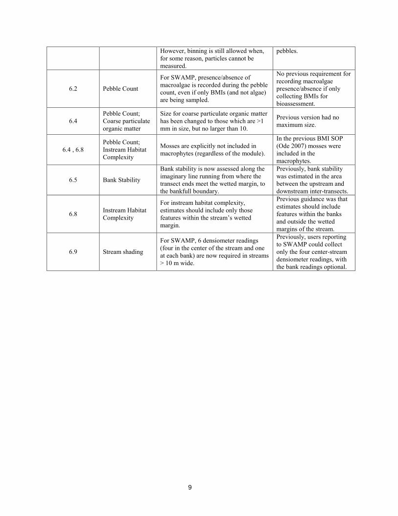
9
However, binning is still allowed when, for some reason, particles cannot be measured.
pebbles.
6.2 Pebble Count
For SWAMP, presence/absence of macroalgae is recorded during the pebble count, even if only BMIs (and not algae) are being sampled.
No previous requirement for recording macroalgae presence/absence if only collecting BMIs for bioassessment.
6.4 Pebble Count; Coarse particulate organic matter
Size for coarse particulate organic matter has been changed to those which are >1 mm in size, but no larger than 10.
Previous version had no maximum size.
6.4 , 6.8 Pebble Count; Instream Habitat Complexity
Mosses are explicitly not included in macrophytes (regardless of the module).
In the previous BMI SOP (Ode 2007) mosses were included in the macrophytes.
6.5 Bank Stability
Bank stability is now assessed along the imaginary line running from where the transect ends meet the wetted margin, to the bankfull boundary.
Previously, bank stability was estimated in the area between the upstream and downstream inter-transects.
6.8 Instream Habitat Complexity
For instream habitat complexity, estimates should include only those features within the stream’s wetted margin.
Previous guidance was that estimates should include features within the banks and outside the wetted margins of the stream.
6.9 Stream shading
For SWAMP, 6 densiometer readings (four in the center of the stream and one at each bank) are now required in streams > 10 m wide.
Previously, users reporting to SWAMP could collect only the four center-stream densiometer readings, with the bank readings optional.
10
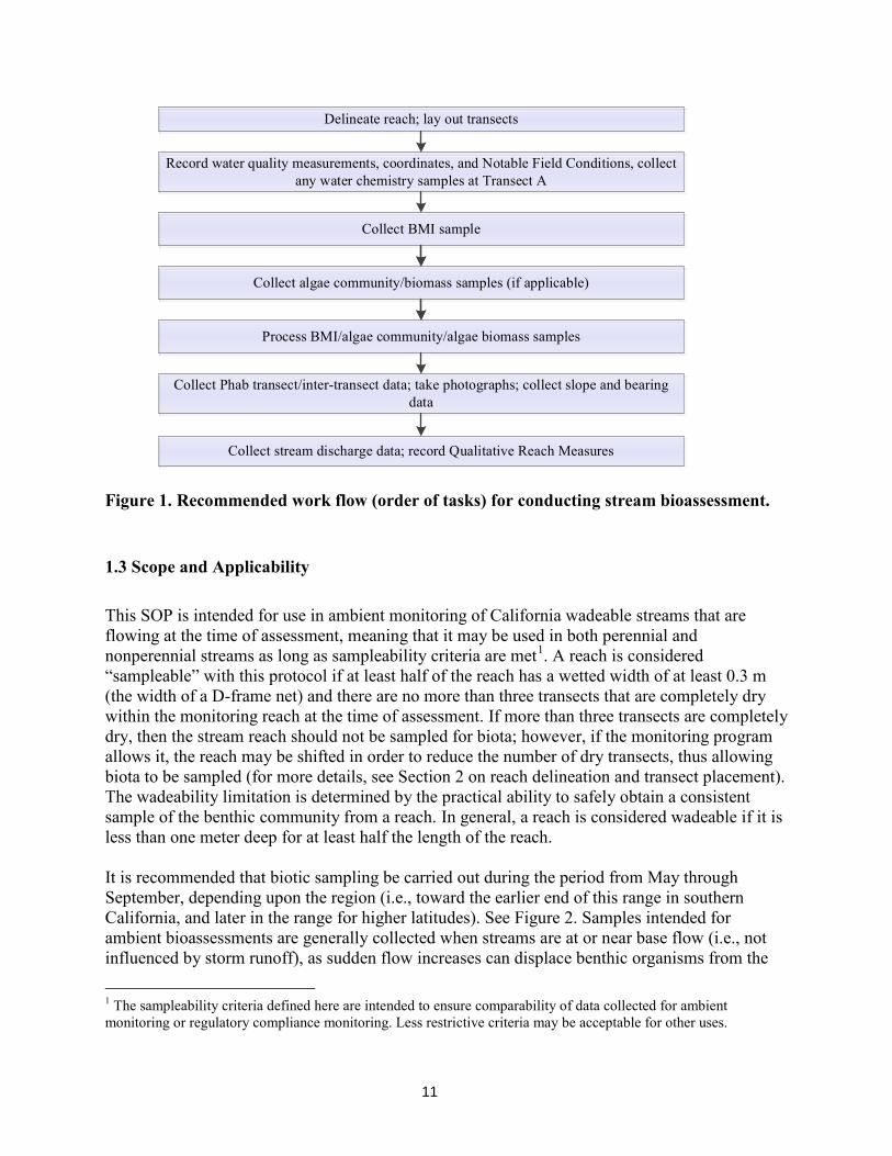
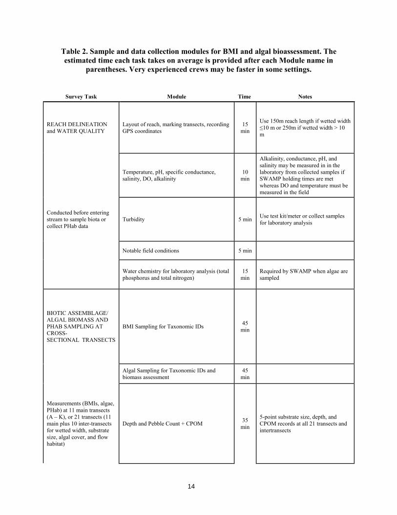
1.2 Sampling Overview This SOP describes methodology for biotic sampling procedures as well as for assessing instream and riparian habitats and ambient water chemistry associated with biotic assemblage samples (Table 2). The sampling layout described in this SOP provides a framework for systematically collecting a variety of biotic, physical, and chemical data. The biotic sampling methods are designed to nest within the overall framework for assessing the biotic, physical, and chemical condition of a reach. The physical habitat characterization methods can be implemented for a stand-alone evaluation or in conjunction with a bioassessment sampling event. This information can be used to characterize stream reaches, associate physical and chemical condition with biotic condition, and explain patterns in the biotic data. Measurements of instream and riparian habitat and ambient water chemistry are essential to interpretation of bioassessment data, and must always accompany bioassessment samples for SWAMP projects. Because bioassessment data requirements vary widely across different applications, this document describes the component measures of instream and riparian habitat as independent “modules”, which may be implemented as needed for each application. For instance, if the goal is to evaluate stream primary production, one may wish to collect only biomass samples and algal cover point-intercept data, and exclude modules focusing on instream habitat complexity. Alternatively, one may need to collect BMI and/or algal taxonomic samples in order to make more refined inferences about stream condition (e.g., by applying a multimetric index based on community composition). Recommendations for modules to include in a reduced-effort (“Basic”) version of this SOP, e.g., for citizen monitoring groups on a limited budget, are provided in the Guidance Document. In order to ensure high-quality bioassessment data, certain tasks must be carried out prior to others. A work-flow diagram depicting the order in which tasks should be undertaken is provided in Figure 1 (see Guidance Document for suggestions to maximize efficiency). Assuming an adequate crew size, the total time required to carry out the full suite of field procedures described in this SOP is approximately 2 to 4 hours in a typical stream, or up to 6 hours in a complex stream. These estimates include only the time spent at the site, not travel time (which varies widely). Table 2 provides a rough breakdown of time requirements per module.
11
Delineate reach; lay out transects
Collect BMI sample
Collect algae community/biomass samples (if applicable)
Process BMI/algae community/algae biomass samples
Collect Phab transect/inter-transect data; take photographs; collect slope and bearing data
Collect stream discharge data; record Qualitative Reach Measures
Record water quality measurements, coordinates, and Notable Field Conditions, collect any water chemistry samples at Transect A
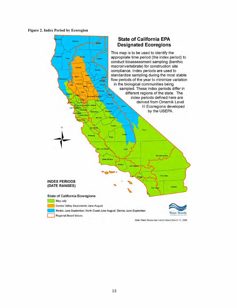
Figure 1. Recommended work flow (order of tasks) for conducting stream bioassessment. 1.3 Scope and Applicability This SOP is intended for use in ambient monitoring of California wadeable streams that are flowing at the time of assessment, meaning that it may be used in both perennial and nonperennial streams as long as sampleability criteria are met1. A reach is considered “sampleable” with this protocol if at least half of the reach has a wetted width of at least 0.3 m (the width of a D-frame net) and there are no more than three transects that are completely dry within the monitoring reach at the time of assessment. If more than three transects are completely dry, then the stream reach should not be sampled for biota; however, if the monitoring program allows it, the reach may be shifted in order to reduce the number of dry transects, thus allowing biota to be sampled (for more details, see Section 2 on reach delineation and transect placement). The wadeability limitation is determined by the practical ability to safely obtain a consistent sample of the benthic community from a reach. In general, a reach is considered wadeable if it is less than one meter deep for at least half the length of the reach. It is recommended that biotic sampling be carried out during the period from May through September, depending upon the region (i.e., toward the earlier end of this range in southern California, and later in the range for higher latitudes). See Figure 2. Samples intended for ambient bioassessments are generally collected when streams are at or near base flow (i.e., not influenced by storm runoff), as sudden flow increases can displace benthic organisms from the
1 The sampleability criteria defined here are intended to ensure comparability of data collected for ambient monitoring or regulatory compliance monitoring. Less restrictive criteria may be acceptable for other uses.
12
stream bottom and dramatically alter local community composition. To be conservative, it is strongly recommended that sampling be carried out at least two, and preferably three, weeks after any storm event that has generated enough stream power to mobilize cobbles and sand/silt capable of scouring stream substrates. See Section 1.4, below, for tips on how to evaluate a site for recent scour. Two to three weeks will usually allow time for benthic fauna and algae to recolonize scoured surfaces (Round 1991; Kelly et al. 1998; Stevenson and Bahls in Barbour et al. 1999). Ultimately, the time of delay from a scouring event to the acceptable window for sampling will depend on environmental setting and time of year. The project manager should consult with the SWAMP bioassessment coordinator in questionable cases. 1.4 Diagnosing Recent Scour As mentioned above, ideally, a stream reach should not be sampled for bioassessment shortly following a scour event that has mobilized bed materials and potentially disrupted benthic communities. However, for certain applications (e.g., wet-weather monitoring), sampling may need to occur under such circumstances. When this happens, a note must be made in the field sheets and the database that flags applicable analytes as having potentially been subjected to recent scour conditions. If a suspected recent scour has occurred, mark “Yes” in the Notable Field Conditions section of the bioassessment field form that says, “Site is affected by recent scouring event”. High-flow/scour indicators that can be assessed to make the determination include:
• Lack of slime/color coating on the streambed (this may be inferred by a high frequency [i.e., near 100%] of microalgal cover scores of “0”; see Section 6.4)
• Lack of macroalgal mats, OR if present, mats displaced, as indicated by being “unnaturally” bunched up against fixed objects within the stream (like tree roots, large boulders) away from centroid of flow
• Non-rigid instream vegetation (e.g., emergent macrophytes like cattails and tules) bent over or lying down within the stream
• Absence of leaves and other detritus in pools, despite riparian cover
Following the sampling visit, under “Field Notes/Comments” on the field sheet, field crews or the project manager can add the size of, and actual time since, storms or discharge releases.
13
Figure 2. Index Period by Ecoregion
14
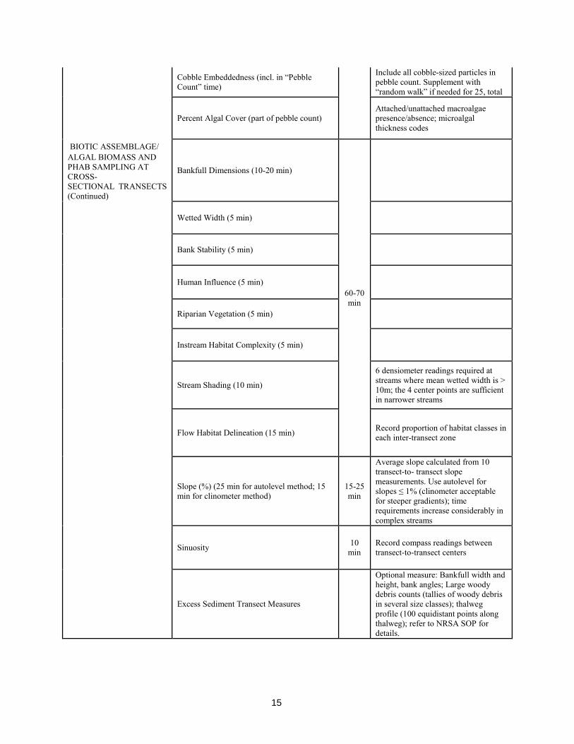
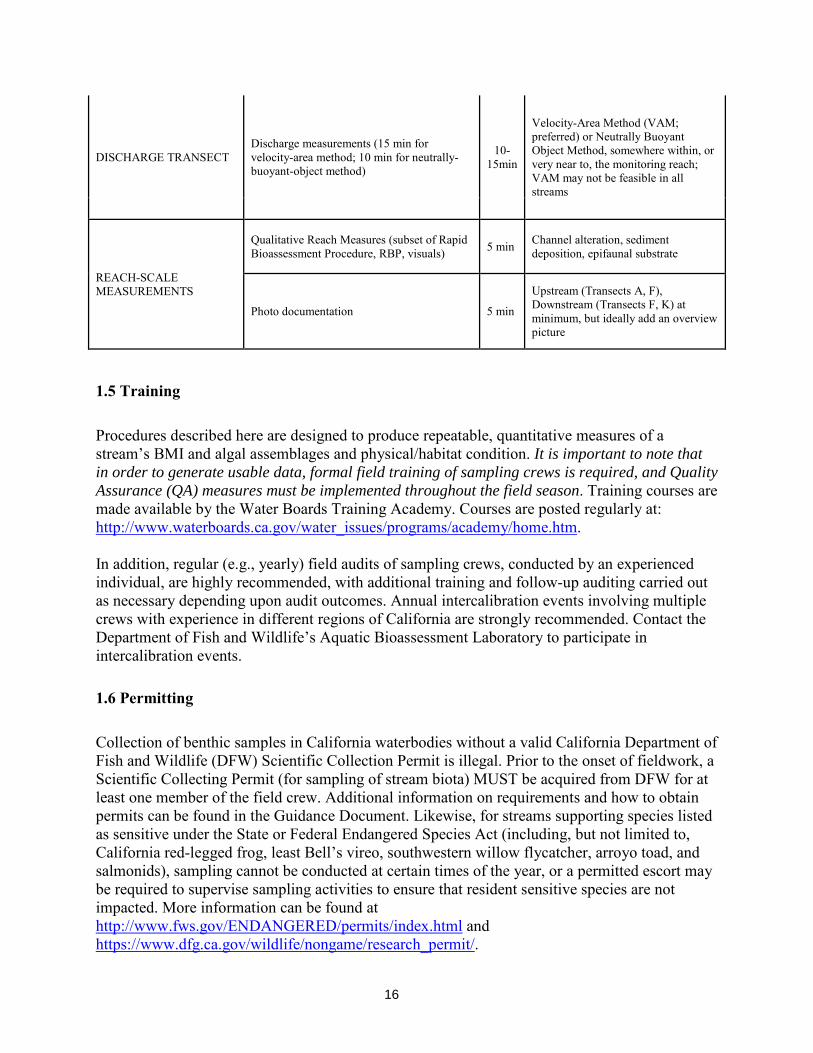
Table 2. Sample and data collection modules for BMI and algal bioassessment. The estimated time each task takes on average is provided after each Module name in
parentheses. Very experienced crews may be faster in some settings.
Survey Task Module Time Notes
REACH DELINEATION and WATER QUALITY
Layout of reach, marking transects, recording GPS coordinates
15 min
Use 150m reach length if wetted width ≤10 m or 250m if wetted width > 10 m
Temperature, pH, specific conductance, salinity, DO, alkalinity
10 min
Alkalinity, conductance, pH, and salinity may be measured in in the laboratory from collected samples if SWAMP holding times are met whereas DO and temperature must be measured in the field
Conducted before entering stream to sample biota or collect PHab data
Turbidity 5 min Use test kit/meter or collect samples for laboratory analysis
Notable field conditions 5 min
Water chemistry for laboratory analysis (total phosphorus and total nitrogen)
15 min
Required by SWAMP when algae are sampled
BIOTIC ASSEMBLAGE/ ALGAL BIOMASS AND PHAB SAMPLING AT CROSS-SECTIONAL TRANSECTS
BMI Sampling for Taxonomic IDs 45 min
Algal Sampling for Taxonomic IDs and biomass assessment
45 min
Measurements (BMIs, algae, PHab) at 11 main transects (A – K), or 21 transects (11 main plus 10 inter-transects for wetted width, substrate size, algal cover, and flow habitat)
Depth and Pebble Count + CPOM 35 min
5-point substrate size, depth, and CPOM records at all 21 transects and intertransects
15
Cobble Embeddedness (incl. in “Pebble Count” time)
Include all cobble-sized particles in pebble count. Supplement with “random walk” if needed for 25, total
Percent Algal Cover (part of pebble count) Attached/unattached macroalgae presence/absence; microalgal thickness codes
BIOTIC ASSEMBLAGE/ ALGAL BIOMASS AND PHAB SAMPLING AT CROSS-SECTIONAL TRANSECTS (Continued)
Bankfull Dimensions (10-20 min)
60-70 min
Wetted Width (5 min)
Bank Stability (5 min)
Human Influence (5 min)
Riparian Vegetation (5 min)
Instream Habitat Complexity (5 min)
Stream Shading (10 min)
6 densiometer readings required at streams where mean wetted width is > 10m; the 4 center points are sufficient in narrower streams
Flow Habitat Delineation (15 min) Record proportion of habitat classes in each inter-transect zone
Slope (%) (25 min for autolevel method; 15 min for clinometer method)
15-25 min
Average slope calculated from 10 transect-to- transect slope measurements. Use autolevel for slopes ≤ 1% (clinometer acceptable for steeper gradients); time requirements increase considerably in complex streams
Sinuosity 10 min
Record compass readings between transect-to-transect centers
Excess Sediment Transect Measures
Optional measure: Bankfull width and height, bank angles; Large woody debris counts (tallies of woody debris in several size classes); thalweg profile (100 equidistant points along thalweg); refer to NRSA SOP for details.
16
DISCHARGE TRANSECT Discharge measurements (15 min for velocity-area method; 10 min for neutrally-buoyant-object method)
10-15min
Velocity-Area Method (VAM; preferred) or Neutrally Buoyant Object Method, somewhere within, or very near to, the monitoring reach; VAM may not be feasible in all streams
REACH-SCALE MEASUREMENTS
Qualitative Reach Measures (subset of Rapid Bioassessment Procedure, RBP, visuals) 5 min Channel alteration, sediment
deposition, epifaunal substrate
Photo documentation 5 min
Upstream (Transects A, F), Downstream (Transects F, K) at minimum, but ideally add an overview picture
1.5 Training Procedures described here are designed to produce repeatable, quantitative measures of a stream’s BMI and algal assemblages and physical/habitat condition. It is important to note that in order to generate usable data, formal field training of sampling crews is required, and Quality Assurance (QA) measures must be implemented throughout the field season. Training courses are made available by the Water Boards Training Academy. Courses are posted regularly at: http://www.waterboards.ca.gov/water_issues/programs/academy/home.htm. In addition, regular (e.g., yearly) field audits of sampling crews, conducted by an experienced individual, are highly recommended, with additional training and follow-up auditing carried out as necessary depending upon audit outcomes. Annual intercalibration events involving multiple crews with experience in different regions of California are strongly recommended. Contact the Department of Fish and Wildlife’s Aquatic Bioassessment Laboratory to participate in intercalibration events. 1.6 Permitting Collection of benthic samples in California waterbodies without a valid California Department of Fish and Wildlife (DFW) Scientific Collection Permit is illegal. Prior to the onset of fieldwork, a Scientific Collecting Permit (for sampling of stream biota) MUST be acquired from DFW for at least one member of the field crew. Additional information on requirements and how to obtain permits can be found in the Guidance Document. Likewise, for streams supporting species listed as sensitive under the State or Federal Endangered Species Act (including, but not limited to, California red-legged frog, least Bell’s vireo, southwestern willow flycatcher, arroyo toad, and salmonids), sampling cannot be conducted at certain times of the year, or a permitted escort may be required to supervise sampling activities to ensure that resident sensitive species are not impacted. More information can be found at http://www.fws.gov/ENDANGERED/permits/index.html and https://www.dfg.ca.gov/wildlife/nongame/research_permit/.

17
1.7 Avoiding the Transfer of Invasive Species and Pathogens Amongst Sites Proper field hygiene must be practiced at all times in order to avoid transferring invasive organisms or pathogens between sites. Examples include, but are not limited to, New Zealand mud snail and chytrid fungus. Before approaching any stream, precautions must be taken to ensure that all equipment that will come into contact with the stream or its immediate surroundings has been properly decontaminated. Such equipment includes, but is not limited to, footwear, D-frame net, algae sampling devices, water chemistry sample fill bottle, transect tape, flags, stadia rod, flow meter, water chemistry probes, and autolevel tripod. Furthermore, under no circumstances shall stream water (e.g., from water bottles used for algae sample processing) or other material collected at one site be introduced into another stream. Detailed information on acceptable decontamination procedures is provided in the Guidance Document. 1.8 SWAMP Requirements The “reachwide benthos” (RWB) sampling procedure, as described in this SOP, is the required sampling method for ambient bioassessment under the SWAMP program. However, other sampling methods (e.g., Targeted Riffle Composite (TRC)) may be desirable if data comparability within long-term monitoring projects that have historically used other methods is sought. In general, SWAMP-funded projects must adhere to the directives of the SWAMP Quality Assurance team as detailed in: Amendment to SWAMP Interim Guidance on Quality Assurance for SWAMP Bioassessments 9-17-08. This memo can be found in the Guidance Document. The project manager must have the approval of the SWAMP Bioassessment Program Lead Scientist and the SWAMP Quality Assurance Officer before the use of alternative methods that deviate from this SOP and the above-referenced memo will be accepted. For other projects and/or programs desiring SWAMP comparability, deviations should be approved by the project manager and project QA officer. SWAMP requires that duplicate sampling of BMIs and benthic algae occur at 10% of study sites (preferably at the same set of sites, when both assemblages are being sampled together). The recommended location for collecting duplicates is at adjacent positions along the sampling transects (described in Section 4). In addition, regular (e.g., yearly) field audits of sampling crews should be conducted by an authorized individual (e.g., qualified personnel of DFW). Note also that SWAMP requires 5% field duplicates for water chemistry measurements. In general, the SWAMP Quality Assurance Program Plan (QAPrP) in place at the time of monitoring or subsequent revisions to that QAPrP and the SMC Bioassessment QAPP (2009) should be followed for quality assurance procedures, when applicable. For more information, refer to: http://www.waterboards.ca.gov/water_issues/programs/swamp/tools.shtml#qa SWAMP participants collecting water-quality and water-chemistry measurements may reference the California Department of Fish and Wildlife - Marine Pollution Studies Laboratory SOP: Collections of Water and Bed Sediment Samples with Associated Field Measurements and Physical Habitat in California. Version 1.1, updated March-2014. This procedure may be used to collect samples for a number of analyses covered by the SWAMP
18
Quality Assurance program. Use of this procedure is a recommendation and not a requirement for SWAMP projects. Prior to sample collection, participants using this procedure shall check its requirements against the latest SWAMP Quality Control and Sample Handling Guidelines. SWAMP is planning to develop additional guidance for bioassessment quality assurance and control procedures. This may include more specific information covering personnel qualifications, training and field audit procedures, procedures for field calibration, procedures for chain of custody documentation, requirements for measurement precision, health and safety warnings, cautions (to avoid actions that would result in instrument damage or compromised samples), and interferences (regarding consequences of not following the SOP). 1.9 Supplemental Guidance A companion document, SWAMP Bioassessment Supplemental Guidance (herein referred to as the “Guidance Document”), is referenced throughout this SOP. It provides more detailed information on the various applications of the modules described here, as well as recommendations for where, when, and/or how to implement the procedures. It also provides suggestions for how to deal with special circumstances that may be encountered during stream bioassessment sampling and more detailed information to aid in interpretation of PHab field indicators. The Guidance Document is a “living” supplement to the field sampling protocol, in the sense that it is regularly updated (unlike this SOP, which is static between versions) and serves as a repository for implementation advice. The Guidance Document is posted on the SWAMP website at Http://www.waterboards.ca.gov/water_issues/programs/swamp/bioassessment/sops.shtml Please check this site regularly in order to review the most recent information on execution of the SOP.
2. REACH DELINEATION AND SCORING NOTABLE FIELD CONDITIONS
Before biotic sample and PHab data collection can begin, the monitoring reach must be identified and delineated, information about reach location and condition is to be documented, water chemistry parameters are to be recorded, and water samples may also be collected. A set of field forms for recording information about monitoring sites, biotic samples, and associated water chemistry and PHab data is available on the SWAMP website at http://www.swrcb.ca.gov/water_issues/programs/swamp/tools.shtml#methods. Field crews using paper forms must designate someone (other than the field recorder) to review the forms for completeness2 and legibility. It is imperative to confirm throughout the data collection effort at each site that all necessary data have been recorded on the field forms correctly by double-checking values and confirming spoken values with field partner(s). All SWAMP data management tools including an electronic data entry interface of the field forms are available 2 If parameters cannot be measured for some reason, "NR" (i.e., “Not Recorded”) should be entered in the corresponding field.
19
from the SWAMP website for use on a portable field computer. Please visit the SWAMP Data Management Resources website for webinar training, tools, templates, and more. http://www.waterboards.ca.gov/water_issues/programs/swamp/data_management_resources/index.shtml A list of supplies needed for sampling and data collection is provided in the Guidance Document.
Step 1. Upon arrival at the site, fill out the “Reach Documentation” section of the field forms. Record the Station Code following SWAMP formats3. Record the geographic coordinates of the downstream end (Transect A) of the reach (in decimal degrees to at least five decimal places) with a Global Positioning System (GPS) receiver and record the datum setting (preferably NAD83) of the unit. Coordinates are to be averaged based on procedures outlined in the GPS device manual. This average is recorded as actual coordinates on field sheet. Target coordinates need to be determined before the field sampling, and should be placed on a map (paper or digital) for visual orientation in case the GPS is not functioning in the field (e.g., in steep canyons or in mountainous regions). Sampling locations for probability sites can be moved up or downstream as much as 300 m from the target location for reasons such as avoiding obstacles, mitigating issues regarding safety or permission to access, and GPS error. If for some reason the GPS measurements for the actual site assessed are not taken at Transect A (e.g., if no GPS signal was available at Transect A), then the actual site location must be noted on the field data sheets. For probabilistically selected sites “target coordinates” are selected at random. Because GIS information about stream locations is imperfect, the target coordinates may not fall exactly on a streambed, but rather nearby, requiring a geospatial shift in order to correspond to the nearest streambed. The potential discrepancy between the target coordinates and where sampling actually occurs makes it essential to record the actual field coordinates on the field sheet. Step 2. To delineate the monitoring reach, first scout it to ensure it is of adequate length for sampling biota. The length to use depends upon the average “wetted width” of the stream reach. The “wetted channel” is the zone that is inundated with water, and “wetted width” is the distance between the sides of the channel at the point where substrates are no longer surrounded by surface water. If the average wetted width ≤ 10 m, delineate a 150 m reach for sampling. If the average wetted width > 10 m, delineate a 250 m reach. When delineating the reach, stay out of the channel as much as possible to avoid disturbing the stream bottom, which could compromise the water and biotic samples, and PHab data, that will subsequently be collected. Starting at one end of the reach, walk along the stream bank, taking large steps (for most adults, a large step is roughly equal to a meter) and count the steps until reaching 150 m (or 250 m for larger streams). This will give a rough idea about the location of the ends of the sampling reach. If the monitoring program affords flexibility in terms of where the sampling reach can be placed, scout for any features that should ideally be excluded (e.g., tributaries, “end-of-pipe” outfalls feeding into the channel, bridge crossings, major changes between natural and artificial channel structures, waterfalls, and impoundments). If any such features are near the target sampling location, and there is not enough room to accommodate a full 150 m reach or 250 m reach 3 Before going in the field, a station code needs to be assigned to each of the sampling sites. For SWAMP-funded projects, please contact the SWAMP database management team for station codes.
20
entirely upstream or downstream of the feature(s), then the reach may be shortened (to as little as 100 m) in order to exclude them. Record on the datasheet under “Actual Reach Length” the length of the reach that has been delineated.
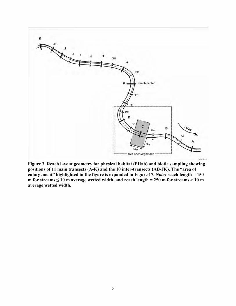
Step 3. Use markers (e.g., wire-stemmed flags) to indicate locations of transects and intertransects. The standard sampling layout consists of 11 “main” transects (A-K) interspersed with 10 “inter-transects”, all of which are arranged perpendicularly to the primary direction of stream flow (usually the thalweg), and placed at equal distances from one to the next (Figure 3). The first flag should be installed at water’s edge on one bank at the downstream limit of the sampling reach to indicate the first main transect (“A”). The positions of the remaining transects and inter-transects are then established by heading upstream along the bank and using the transect tape or a segment of rope of appropriate length to measure off successive segments of 7.5 m (if sampling reach is 150 m), or 12.5 m (if it is 250 m). 4
Step 4. Under “Notable Field Conditions”, record evidence of recent flooding, fire, or other disturbances that might influence bioassessment samples, such as scour, for which specific guidance is provided in Section 1.4, above. These are subjective determinations, so use whatever cues are available to make the call. If unaware of recent fire or rainfall events, select the “no” option on the form. Also, to the best of your ability, record the dominant land use and land cover in the area surrounding the reach (i.e., evaluate land cover within 50 m of either side of the stream reach). Use a scaled aerial photograph of the site and vicinity as an aid. Finally, mark whether or not the sampling reach occurs within an engineered channel5.
4 Although it is usually easiest to establish transect positions from the banks (this also prevents disturbance to the stream channel), this can result in uneven spacing of transects in complex stream reaches. To avoid this, estimate transect positions by projecting from the mid-channel to the banks. Refer to Figure 3 for a visual clarification of proper transect alignment relative to the stream’s direction of flow. For monitoring reaches of non-standard length (i.e., < 150 m; see Step 2 above), divide the total length of the reach by 20 to derive the distance between the adjacent main, and inter-, transects. Alternating between two different flag colors (e.g., orange and yellow, or blue), to demarcate main- vs. inter-transects is recommended, as well as writing the transect/inter-transects names on the flags. 5 Engineered channels include streams that have been straightened or armored (with riprap, rocks, grout, concrete, or earthen levees) on the banks, streambed, or floodplain of the channel. Partially armored channels (e.g., armored only at bridge abutments) are considered to be “engineered”.
21
Figure 3. Reach layout geometry for physical habitat (PHab) and biotic sampling showing positions of 11 main transects (A-K) and the 10 inter-transects (AB-JK). The “area of enlargement” highlighted in the figure is expanded in Figure 17. Note: reach length = 150 m for streams ≤ 10 m average wetted width, and reach length = 250 m for streams > 10 m average wetted width.
22
3. WATER CHEMISTRY SAMPLING
Before entering the stream to sample water, remember to adhere to proper field hygiene practices (see Section 1.7 for more details) at all times. In addition, be sure to sample water in such a way that it does not interfere with subsequent biotic sampling and PHab data collection, but also in such a way that water samples are not compromised by other sampling activities upstream (e.g., by suspension of matter from the stream bottom into the water column, and the consequent introduction of this matter into the water chemistry samples). All water chemistry/toxicology samples should be collected prior to stepping in the water anywhere upstream of the water/toxicology sampling spot and should not be collected in a location where subsequent biotic samples or PHab data are to be collected. Sampling water chemistry just downstream of Transect A, the same general location as where the GPS coordinates were taken6, and before any other sampling activities take place, achieves both of these goals.
Step 1. Calibrate probes as necessary (some require daily calibration) and record the calibration date on the field form. For calibration procedures, follow the SWAMP QAPrP in place at the time of monitoring or subsequent revisions to that QAPrP (http://www.waterboards.ca.gov/water_issues/programs/swamp/tools.shtml#qa), or the manufacturer’s guidelines, whatever is more stringent. Field measurements in this SOP are typically taken with a handheld water-quality meter (e.g., YSI, Hydrolab), but field test kits (e.g., Hach) may provide acceptable information as well.
Step 2. Measure and record common ambient water-chemistry parameters7:
• Turbidity (NTU) • Water temperature (°C) • Specific conductivity (µS/cm) • Salinity (ppt) • Alkalinity (mg/L) • pH • Dissolved oxygen (mg/L and % saturation)
Because it may be affected by disturbance of the streambed that occurs during sampling, measure turbidity (if applicable) first. If water samples are also to be collected, such sampling should also occur at this location and time, and collection should also precede probe measurements. Measurements and water chemistry sample collection should take place in areas with flowing water, avoiding depositional zones (e.g., pools), if possible.
6 If, for whatever reason, measurements are not taken at Transect A before biotic sampling in the reach has begun, they should be taken immediately upstream of Transect K (the most undisturbed transect), and this change of sampling location should be noted on the field sheet. 7 SWAMP-required ambient water chemistry parameters measured in the field are: pH, DO, specific conductivity, salinity, alkalinity, and water temperature. Samples for all other ambient water chemistry should be analyzed in the laboratory (except for silica, which can be measured in the field with kits or in the laboratory). Turbidity and silica are optional measurements for SWAMP purposes.
23
Turbidity can be measured with a multi-probe (e.g., YSI) or a turbidimeter, or it can be analyzed in the laboratory. If using a portable meter, collect approximately 250 mL of water for turbidity measurements approximately 10 cm below the water surface (if possible), and take two separate readings from subsamples of the same grab sample and report the average. Likewise, all probe measurements should be made 10 cm below the water surface. Alkalinity (mg/L) may be measured with a field test kit (e.g. Hach AL-AP #2444301) or in the laboratory. A digital titrator (e.g., Hach) using low-concentration acid (such as 0.16N H2SO4) as the titrant is recommended for determining alkalinity in low-alkalinity streams (i.e., < ~100 mg/L CaCO3). If algae samples are being collected, SWAMP requires that samples also be collected for analysis of water-column total nitrogen (TN) and total phosphorus (TP); nitrate-nitrite, and orthophosphate are also recommended. TN/TP samples should not be filtered. Sample holding times, field preparation, bottle types, and recommended volumes for each water-chemistry analyte can be found in the Quality Control and Sample Handling Guidelines 8 (http://www.waterboards.ca.gov/water_issues/programs/swamp/tools.shtml#field). Greater detail on field sampling methods for water chemistry can be found at: http://www.waterboards.ca.gov/water_issues/programs/swamp/docs/final_collect_water_sed_phys_habitat.pdf.
8 Crews can opt to collect water at the end of sampling for holding time purposes, in which case sampling should be conducted in undisturbed water.
24
4. BIOTIC COMMUNITY SAMPLING
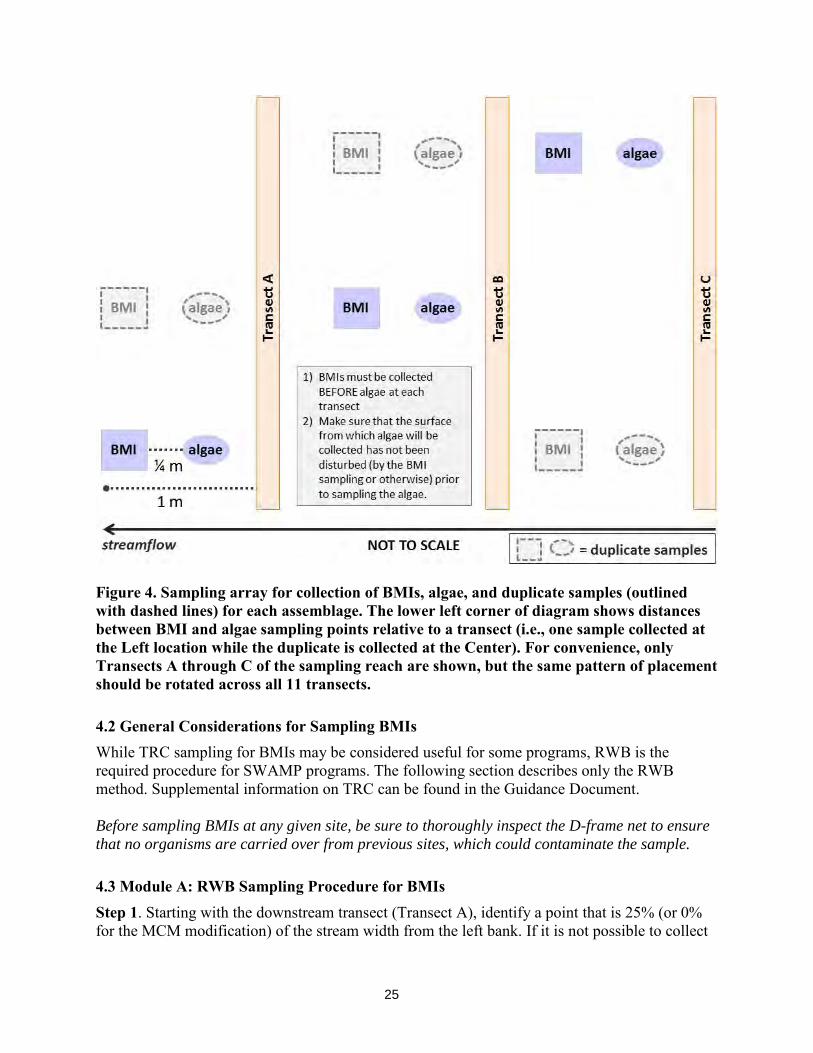
Once the transects have been laid out and water sampling is complete, the biotic samples (BMIs and/or algae) can be collected. On a transect-by-transect basis, any biotic sampling should occur before PHab data are collected, and BMIs should always be collected before algae because BMIs are often highly motile and could be flushed by the algae sampling activity. 4.1 The Reachwide Benthos (RWB) Method for Biotic Sample Collection The RWB procedure employs an objective method for selecting subsampling locations that is built upon the layout of the 11 main transects that will be also used for physical habitat measurements. This method can be used to sample any wadeable stream reach, since it does not target specific habitats. Because sampling locations are defined by the transect layout, the position of individual sub-samples may fall in a variety of “erosional9” or “depositional10” habitats. For the RWB method, the sub-sampling position alternates between left, center, and right portions of the main transects, as one proceeds upstream from one transect to the next. These sampling locations are defined as the points at 25% (“left11”), 50% (“center”) and 75% (“right”) across the wetted width in most systems. The left and right sides of the stream are determined when facing downstream. SWAMP programs should employ a modified version of the RWB method, called the Margin-Center-Margin (MCM) method when all three of the following stream conditions are met: 1) very low slope (generally < ~ 0.3%); 2) uniform sandy/fine-substrate; and 3) stable habitat at stream margins. The MCM protocol modification is to collect subsamples at 0%, 50%, and 100% of wetted width instead of 25%, 50%, and 75%, to ensure collection of biota from marginal habitats. There is no hard rule for using the MCM variation, but in general it should be reserved for reaches where the bulk of the streambed consists of unstable habitat (e.g., shifting sands), and the only stable microhabitats (e.g., macrophytes, algae) are restricted to the margins and would otherwise be missed. The type of sampling method used (RWB, MCM, or TRC) should be circled on the field sheet under “collection method”. The recommended method for collecting duplicate biotic samples is at adjacent positions along the sampling transects according to the scheme depicted in Figure 3 (the duplicates are shown in light grey, with dashed-line outlines). Both samples should be collected at each transect before moving on to the next transect.
9 Erosional – habitats in the stream that are dominated by fast-moving water, such as riffles, where stream power is more likely to facilitate erosion (suspension) of loose benthic material than deposition; examples of “erosional” substrates include cobbles and boulders. 10 Depositional – habitats in the stream that are dominated by slow-moving water, such as pools, where deposition of materials from the water column is more likely to occur than erosion (or (re)suspension) of bed materials; examples of “depositional” substrates include silt and sand. 11 Conventionally, “left bank” has been defined as the left bank when facing downstream (i.e., in the direction of the current).
25
Figure 4. Sampling array for collection of BMIs, algae, and duplicate samples (outlined with dashed lines) for each assemblage. The lower left corner of diagram shows distances between BMI and algae sampling points relative to a transect (i.e., one sample collected at the Left location while the duplicate is collected at the Center). For convenience, only Transects A through C of the sampling reach are shown, but the same pattern of placement should be rotated across all 11 transects. 4.2 General Considerations for Sampling BMIs While TRC sampling for BMIs may be considered useful for some programs, RWB is the required procedure for SWAMP programs. The following section describes only the RWB method. Supplemental information on TRC can be found in the Guidance Document. Before sampling BMIs at any given site, be sure to thoroughly inspect the D-frame net to ensure that no organisms are carried over from previous sites, which could contaminate the sample. 4.3 Module A: RWB Sampling Procedure for BMIs Step 1. Starting with the downstream transect (Transect A), identify a point that is 25% (or 0% for the MCM modification) of the stream width from the left bank. If it is not possible to collect
26
a sample at the designated point because of deep water, obstacles, or unsafe conditions, adjust the sampling spot while keeping the point as close as possible to the designated position. Always be as objective as possible when identifying the sampling spot; resist the urge to sample the “best looking” or most convenient area of the streambed. Step 2. Once the sampling spot is identified, place the 500-µm D-frame net in the water 1 m downstream of the target transect. In order to avoid affecting subsequent PHab data collection, do not sample directly on the transect. Position the net so its mouth is perpendicular to, and facing into, the flow of the water. If there is sufficient current in the area at the sampling spot to fully extend the net, use the normal D-net collection technique (as described in steps 3-6 below) to collect the sub-sample.12 Step 3. Holding the net in position on the substrate, visually define a square shape (a “sampling plot”) on the stream bottom upstream of the net opening, approximately one net-width wide and one net-width long. Because standard D-nets are 12 inches wide, the area within this plot is 1ft2 (0.09 m2). Restrict sampling to within that area. Step 4. Working backward from the upstream edge of the sampling plot, check the sampling plot for heavy organisms such as mussels, caddis cases, and snails. Remove these organisms from the substrate by hand and place them into the net. Carefully pick up and rub stones directly in front of the net to remove attached animals. Pick up and clean all of the rocks larger than a golf ball within the sampling plot such that all the organisms attached to them are washed downstream into the net. Set these rocks outside the sampling plot after they have been cleaned. Large rocks that protrude less than halfway into the sampling area should be pushed aside. If the substrate is consolidated, bedrock, or comprised of large, heavy rocks, kick and dislodge the substrate (with the feet) to displace BMIs into the net. If a rock cannot be removed from the stream bottom, rub it with your hands or feet (concentrating on cracks or indentations), thereby loosening any attached insects. While disturbing the plot, let the water current carry all loosened material into the net. Do not use a brush to dislodge organisms from substrates. Step 5. Once the coarser substrates have been removed from the sampling plot, dig through the remaining underlying material with fingers or a digging tool (e.g., rebar or an abalone iron) to a depth of about 10 cm (less in sandy streams), where gravels and finer particles are often dominant. Thoroughly manipulate the substrates in the plot to encourage flow to dislodge any resistant organisms. Note: the sampler may spend as much time as necessary to inspect and clean larger substrates, but should take a standard time of 30 seconds for the digging portion of this step. To the extent practical, reduce the amount of sand particles in the net, as they damage organisms and degrade taxonomic data quality.
12 When sampling in slack water and flow volume is insufficient to use a D-frame net to capture dislodged BMIs drifting downstream, spend 30 seconds hand picking a sample from 1ft2 area of substrate at the sampling location. Then stir up the substrate with gloved hands and use a sieve with 500-µm mesh size to collect the organisms from the water in the same way the net is used in larger pools to wash the organisms to the bottom of the net.
27
For slack-water habitats, vigorously kick the remaining finer substrate within the plot using the feet while dragging the net repeatedly through the disturbed area just above the bottom. Keep moving the net so that the organisms trapped in the net will not escape. Continue kicking the substrate and moving the net for 30 seconds. For vegetation-choked sampling points, sweep the net through the vegetation within a 1-ft2 (0.09 m2) plot for 30 seconds. After 30 seconds, remove the net from the water with a quick, upward motion to wash the organisms to the bottom of the net. Step 6. Let the water run clear before carefully lifting the net. Dip the lower portion of net in the stream several times to remove fine sediments and to concentrate organisms into the end of the net, while being careful to prevent water or foreign material from entering the mouth of the net. Be particularly careful to avoid “backflow” situations, in which collected material restricts flow through the net and the resulting turbulent flow causes collected material to escape the net; this is a major potential source of loss of BMIs during sampling. Step 7 Move on to the next transect to repeat the sampling process across all 11 main transects. The sampling position within each transect is alternated between the left, center, and right positions along a transect (25%, 50%, and 75% of wetted width, respectively, for standard RWB, or 0%, 50%, and 100% if using the MCM collection method), then cycling through the same order over and over again while moving upstream from transect to transect. Ultimately, you will collect from the left and center 4 times each, and the right 3 times. 13 Step 8. Fill and label sample jars. Once all 11 subsamples have been collected, proceed to Section 5.1 “Processing Benthic Macroinvertebrate Samples”. 4.4 General Considerations for Sampling Benthic Algae The following is a short introduction to several types of algal indicators that can be monitored as part of a bioassessment effort. For a more detailed discussion, see Fetscher and McLaughlin (2008). The most appropriate indicators to include in a given program will ultimately depend upon that program’s goals, because the various indicators provide information at varying levels of resolution and applicability to different uses. Likewise, the various indicators require different levels of investment in terms of fieldwork and laboratory work. Percent algal cover, for instance, is a rapid means of estimating algal primary production that can be carried out entirely in the field and is conducted in tandem with the PHab pebble count. Therefore, the percent algal cover is an appropriate, fast, and inexpensive parameter for citizen monitoring groups if they are concerned about increased algal biomass. Other estimators of algal biomass include chlorophyll a and AFDM, which involve quantitative collection of algae, preservation, and subsequent laboratory analysis. Algal biomass is a key component of the California Nutrient Numeric Endpoints (NNE) framework (Tetra Tech 2006). Higher resolution taxonomic information about algal assemblages can be used in algal Indices of Biotic Integrity (IBIs; e.g., Fetscher et al. 2014), and offers more in-depth insight into water quality. For this type of data, algal specimens
13Care should be taken in transporting samples between reaches. The use of a reachwide sample bucket can help minimize any possible sample loss. Samples from each transect can be placed in the bucket for transport. This method would be similar to the reach wide sample bucket used for algae sampling.
28
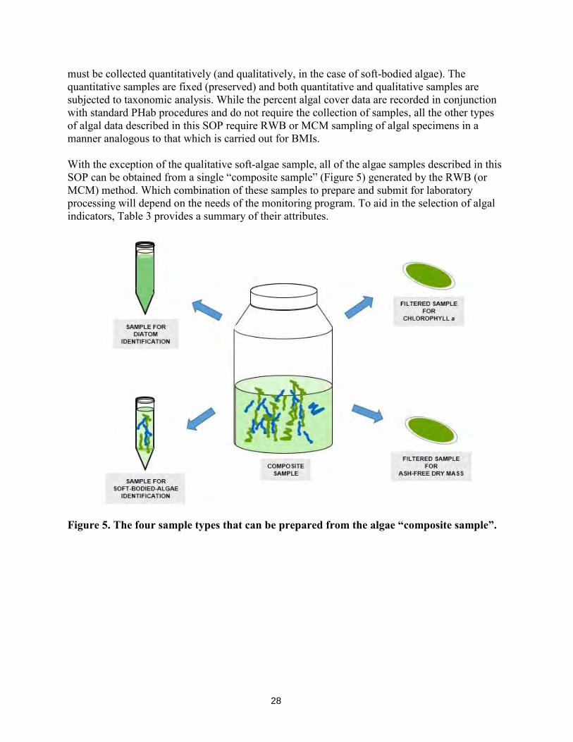
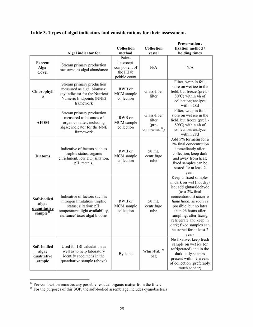
must be collected quantitatively (and qualitatively, in the case of soft-bodied algae). The quantitative samples are fixed (preserved) and both quantitative and qualitative samples are subjected to taxonomic analysis. While the percent algal cover data are recorded in conjunction with standard PHab procedures and do not require the collection of samples, all the other types of algal data described in this SOP require RWB or MCM sampling of algal specimens in a manner analogous to that which is carried out for BMIs. With the exception of the qualitative soft-algae sample, all of the algae samples described in this SOP can be obtained from a single “composite sample” (Figure 5) generated by the RWB (or MCM) method. Which combination of these samples to prepare and submit for laboratory processing will depend on the needs of the monitoring program. To aid in the selection of algal indicators, Table 3 provides a summary of their attributes.
Figure 5. The four sample types that can be prepared from the algae “composite sample”.
29
Table 3. Types of algal indicators and considerations for their assessment.
Algal indicator for Collection
method Collection
vessel
Preservation / fixation method /
holding times
Percent Algal Cover
Stream primary production measured as algal abundance
Point-intercept
component of the PHab
pebble count
N/A N/A
Chlorophyll a
Stream primary production measured as algal biomass;
key indicator for the Nutrient Numeric Endpoints (NNE)
framework
RWB or MCM sample
collection
Glass-fiber filter
Filter, wrap in foil, store on wet ice in the
field, but freeze (pref. -80ºC) within 4h of collection; analyze
within 28d
AFDM
Stream primary production measured as biomass of
organic matter, including algae; indicator for the NNE
framework
RWB or MCM sample
collection
Glass-fiber filter (pre-
combusted14)
Filter, wrap in foil, store on wet ice in the
field, but freeze (pref. -80ºC) within 4h of collection; analyze
within 28d
Diatoms
Indicative of factors such as trophic status, organic
enrichment, low DO, siltation, pH, metals.
RWB or MCM sample
collection
50 mL centrifuge
tube
Add 5% formalin for a 1% final concentration
immediately after collection; keep dark and away from heat; fixed samples can be stored for at least 2
years
Soft-bodied algae
quantitative sample15
Indicative of factors such as nitrogen limitation/ trophic
status; siltation; pH; temperature, light availability, nuisance/ toxic algal blooms
RWB or MCM sample
collection
50 mL centrifuge
tube
Keep unfixed samples in dark on wet (not dry) ice; add glutaraldehyde
(to a 2% final concentration) under a fume hood, as soon as possible, but no later than 96 hours after
sampling; after fixing, refrigerate and keep in dark; fixed samples can be stored for at least 2
years
Soft-bodied algae
qualitative sample
Used for IBI calculation as well as to help laboratory identify specimens in the
quantitative sample (above)
By hand Whirl-PakTM bag
No fixative; keep fresh sample on wet ice (or
refrigerated) and in the dark; tally species
present within 2 weeks of collection (preferably
much sooner) 14 Pre-combustion removes any possible residual organic matter from the filter. 15 For the purposes of this SOP, the soft-bodied assemblage includes cyanobacteria
30
During all phases of algae sampling and processing, in order to preserve specimen integrity, every attempt should be made to keep the sample material out of the sun, and in general, to protect the algae from heat and desiccation, as much as possible. This is necessary in order to reduce the risk of chlorophyll a degradation, limit cell division post-collection, and curb the decay of soft-bodied algae (especially for the fresh qualitative samples; see Section 4.6, “Procedure for Collecting and Storing Qualitative Benthic Algal Samples”). 4.5 Module B: RWB Sampling Procedure for Benthic Algae – Quantitative Samples As with the RWB and MCM methods for BMIs, a quantitative subsample of benthic algae is collected at each of the 11 main transects, and these are combined into a single composite sample. Up to four aliquots are then drawn from the composite sample, and these can be used for analysis of the following: diatom assemblage, soft-bodied algae assemblage, benthic chlorophyll a concentration, and benthic AFDM concentration. A qualitative sample of soft bodied algae is collected in addition to the quantitative sample (see Section 4.6, below). Also, as with BMIs (see Section 4.3, Step 1; and Fig. 4), algae sample collection should begin at Transect A and proceed upstream to Transect K, rotating through the “left”, “center”, “right”, “left”, etc. positions along the 11 main transects. At each transect, BMIs must be collected before algae in order to minimize the chances of disturbing BMIs (potentially causing some to flee the area) during collection of algae. It is likewise important to make sure that the surface from which algae will be collected has not been recently disturbed (by the BMI sampling, or otherwise) prior to sampling the algae. After the BMIs are collected at a given spot, the algae sample should be taken ¼ m upstream from the center of the upper edge of the scar in the stream bottom left from the BMI sampling, according to the schematic in Figure 3. The best way to guarantee that BMI sampling does not interfere with algae sampling is for the person sampling algae to witness exactly where the BMI collector is disturbing the stream bottom in the process of sampling the BMIs. One should not rely upon guessing where the BMIs were collected in order to determine this. Sometimes the "scar" where BMIs were collected will be obvious, but often it will not. If only algae (and not BMIs) are being collected, then the specimens should be collected 1 m downstream of the transects. If only algae (and not BMIs) are being collected in a low-slope reach in which the MCM method is employed, the collection location should be 1 m downstream of the main transect and, for each of the “margin” positions, at a distance of 15 cm (i.e., ½ the width of a D-frame net) inward from the wetted margin of the bank. To ensure that samples of the stream’s algal community and algal biomass concentration are representative of the sampling reach, samples should always be collected by centering the sampling device on the specific point indicated in the above guidelines (i.e., resisting the urge to subjectively choose where to sample). This is particularly important for yielding a representative biomass sample, because subjectively choosing or avoiding spots with high or low levels of algal growth can easily bias the results. Because in the RWB and MCM methods, subsample locations are objectively defined by the transect layout, the position of individual subsampling points may fall within a variety different types of habitats, each of which has implications for the type of substrate likely to be encountered and therefore the type of algae sampling device to use. When confronted with a
31
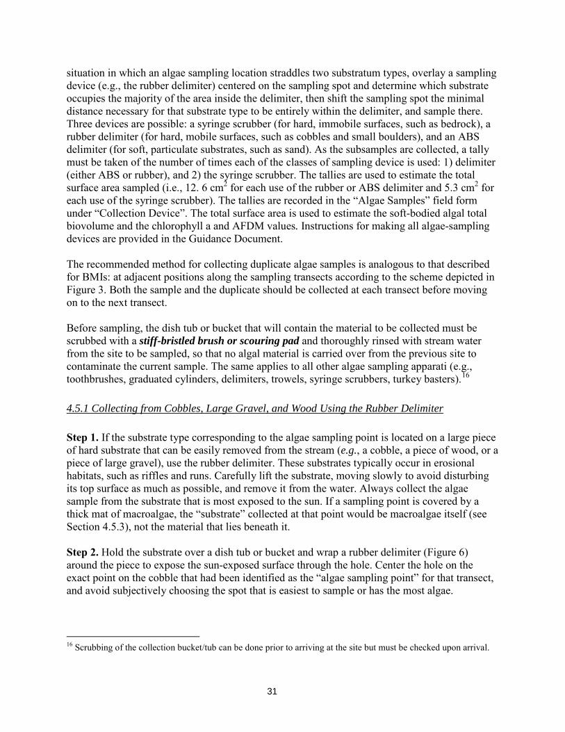
situation in which an algae sampling location straddles two substratum types, overlay a sampling device (e.g., the rubber delimiter) centered on the sampling spot and determine which substrate occupies the majority of the area inside the delimiter, then shift the sampling spot the minimal distance necessary for that substrate type to be entirely within the delimiter, and sample there. Three devices are possible: a syringe scrubber (for hard, immobile surfaces, such as bedrock), a rubber delimiter (for hard, mobile surfaces, such as cobbles and small boulders), and an ABS delimiter (for soft, particulate substrates, such as sand). As the subsamples are collected, a tally must be taken of the number of times each of the classes of sampling device is used: 1) delimiter (either ABS or rubber), and 2) the syringe scrubber. The tallies are used to estimate the total surface area sampled (i.e., 12. 6 cm2 for each use of the rubber or ABS delimiter and 5.3 cm2 for each use of the syringe scrubber). The tallies are recorded in the “Algae Samples” field form under “Collection Device”. The total surface area is used to estimate the soft-bodied algal total biovolume and the chlorophyll a and AFDM values. Instructions for making all algae-sampling devices are provided in the Guidance Document. The recommended method for collecting duplicate algae samples is analogous to that described for BMIs: at adjacent positions along the sampling transects according to the scheme depicted in Figure 3. Both the sample and the duplicate should be collected at each transect before moving on to the next transect. Before sampling, the dish tub or bucket that will contain the material to be collected must be scrubbed with a stiff-bristled brush or scouring pad and thoroughly rinsed with stream water from the site to be sampled, so that no algal material is carried over from the previous site to contaminate the current sample. The same applies to all other algae sampling apparati (e.g., toothbrushes, graduated cylinders, delimiters, trowels, syringe scrubbers, turkey basters).16 4.5.1 Collecting from Cobbles, Large Gravel, and Wood Using the Rubber Delimiter Step 1. If the substrate type corresponding to the algae sampling point is located on a large piece of hard substrate that can be easily removed from the stream (e.g., a cobble, a piece of wood, or a piece of large gravel), use the rubber delimiter. These substrates typically occur in erosional habitats, such as riffles and runs. Carefully lift the substrate, moving slowly to avoid disturbing its top surface as much as possible, and remove it from the water. Always collect the algae sample from the substrate that is most exposed to the sun. If a sampling point is covered by a thick mat of macroalgae, the “substrate” collected at that point would be macroalgae itself (see Section 4.5.3), not the material that lies beneath it. Step 2. Hold the substrate over a dish tub or bucket and wrap a rubber delimiter (Figure 6) around the piece to expose the sun-exposed surface through the hole. Center the hole on the exact point on the cobble that had been identified as the “algae sampling point” for that transect, and avoid subjectively choosing the spot that is easiest to sample or has the most algae.
16 Scrubbing of the collection bucket/tub can be done prior to arriving at the site but must be checked upon arrival.
32
Figure 6. Rubber delimiter
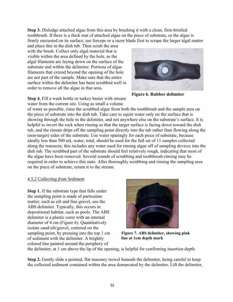
Step 3. Dislodge attached algae from this area by brushing it with a clean, firm-bristled toothbrush. If there is a thick mat of attached algae on the piece of substrate, or the algae is firmly encrusted on its surface, use forceps or a razor blade first to scrape the larger algal matter and place this in the dish tub. Then scrub the area with the brush. Collect only algal material that is visible within the area defined by the hole, as the algal filaments are laying down on the surface of the substrate and within the delimiter. Portions of algae filaments that extend beyond the opening of the hole are not part of the sample. Make sure that the entire surface within the delimiter has been scrubbed well in order to remove all the algae in that area. Step 4. Fill a wash bottle or turkey baster with stream water from the current site. Using as small a volume of water as possible, rinse the scrubbed algae from both the toothbrush and the sample area on the piece of substrate into the dish tub. Take care to squirt water only on the surface that is showing through the hole in the delimiter, and not anywhere else on the substrate’s surface. It is helpful to invert the rock when rinsing so that the target surface is facing down toward the dish tub, and the rinsate drips off the sampling point directly into the tub rather than flowing along the (non-target) sides of the substrate. Use water sparingly for each piece of substrate, because ideally less than 500 mL water, total, should be used for the full set of 11 samples collected along the transects; this includes any water used for rinsing algae off of sampling devices into the dish tub. The scrubbed part of the substrate should feel relatively rough, indicating that most of the algae have been removed. Several rounds of scrubbing and toothbrush-rinsing may be required in order to achieve this state. After thoroughly scrubbing and rinsing the sampling area on the piece of substrate, return it to the stream. 4.5.2 Collecting from Sediment Step 1. If the substrate type that falls under the sampling point is made of particulate matter, such as silt and fine gravel, use the ABS delimiter. Typically, this occurs in depositional habitat, such as pools. The ABS delimiter is a plastic corer with an internal diameter of 4 cm (Figure 6). Quantitatively isolate sand/silt/gravel, centered on the sampling point, by pressing into the top 1 cm of sediment with the delimiter. A brightly colored line painted around the periphery of the delimiter, at 1 cm above the lip of the opening, is helpful for confirming insertion depth. Step 2. Gently slide a pointed, flat masonry trowel beneath the delimiter, being careful to keep the collected sediment contained within the area demarcated by the delimiter. Lift the delimiter,
Figure 7. ABS delimiter, showing pink line at 1cm depth mark
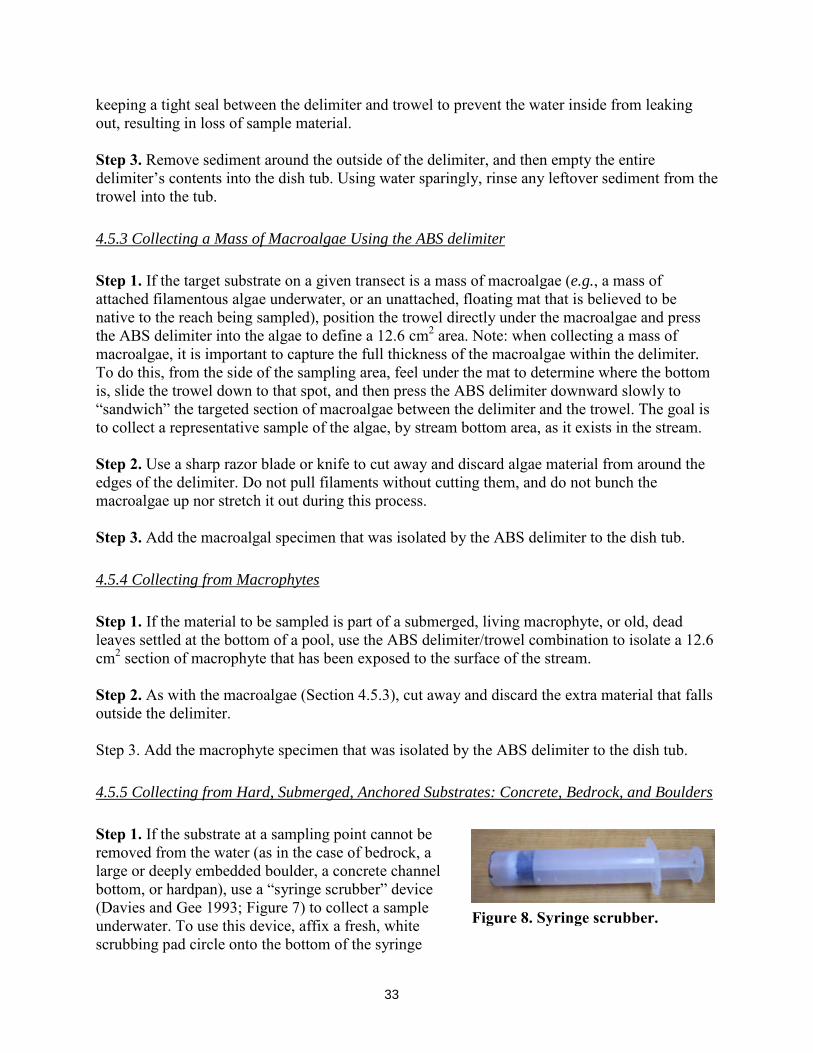
33
keeping a tight seal between the delimiter and trowel to prevent the water inside from leaking out, resulting in loss of sample material. Step 3. Remove sediment around the outside of the delimiter, and then empty the entire delimiter’s contents into the dish tub. Using water sparingly, rinse any leftover sediment from the trowel into the tub. 4.5.3 Collecting a Mass of Macroalgae Using the ABS delimiter Step 1. If the target substrate on a given transect is a mass of macroalgae (e.g., a mass of attached filamentous algae underwater, or an unattached, floating mat that is believed to be native to the reach being sampled), position the trowel directly under the macroalgae and press the ABS delimiter into the algae to define a 12.6 cm2 area. Note: when collecting a mass of macroalgae, it is important to capture the full thickness of the macroalgae within the delimiter. To do this, from the side of the sampling area, feel under the mat to determine where the bottom is, slide the trowel down to that spot, and then press the ABS delimiter downward slowly to “sandwich” the targeted section of macroalgae between the delimiter and the trowel. The goal is to collect a representative sample of the algae, by stream bottom area, as it exists in the stream. Step 2. Use a sharp razor blade or knife to cut away and discard algae material from around the edges of the delimiter. Do not pull filaments without cutting them, and do not bunch the macroalgae up nor stretch it out during this process. Step 3. Add the macroalgal specimen that was isolated by the ABS delimiter to the dish tub. 4.5.4 Collecting from Macrophytes Step 1. If the material to be sampled is part of a submerged, living macrophyte, or old, dead leaves settled at the bottom of a pool, use the ABS delimiter/trowel combination to isolate a 12.6 cm2 section of macrophyte that has been exposed to the surface of the stream. Step 2. As with the macroalgae (Section 4.5.3), cut away and discard the extra material that falls outside the delimiter. Step 3. Add the macrophyte specimen that was isolated by the ABS delimiter to the dish tub. 4.5.5 Collecting from Hard, Submerged, Anchored Substrates: Concrete, Bedrock, and Boulders Step 1. If the substrate at a sampling point cannot be removed from the water (as in the case of bedrock, a large or deeply embedded boulder, a concrete channel bottom, or hardpan), use a “syringe scrubber” device (Davies and Gee 1993; Figure 7) to collect a sample underwater. To use this device, affix a fresh, white scrubbing pad circle onto the bottom of the syringe
Figure 8. Syringe scrubber.
34
plunger using the Velcro hooks on the end of the plunger. Submerge the device in the stream and work the plunger up and down a couple times to lubricate it. Then press the plunger down so that the bottom of the scrubbing pad is flush with the bottom of the barrel. Step 2. Submerge the syringe in the stream again, this time pressing the syringe bottom firmly against the substrate, centered on the sampling point. Once a good seal with the substrate is achieved, rotate the syringe scrubber completely 3 times in order to collect the biofilm from the substrate surface onto the pad. If the surface of the substrate where the sampling point fell is not flat enough to allow for a tight seal with the syringe barrel, move the collection point to the nearest area that is sufficiently flat and collect the sample there. Step 3. After rotating the syringe scrubber, and before removing it from the substrate, gently retract the plunger slightly (e.g., <5 mm), so that the pad is no longer touching the substrate, but not so much that a lot of water enters the barrel. Carefully slide the trowel under syringe barrel, slightly tilting the barrel to allow the trowel to enter. If there is a strong current, lift the downstream side of the barrel. Then pull the instrument back out of the water with the trowel still firmly sealed against the syringe-barrel bottom. Step 4. Hold the syringe scrubber over the dish tub and remove the trowel, allowing any water that was between the trowel and the scrubber pad to fall into the tub (but discard the water inside the plunger-handle end of the barrel—there is no need to add this water to the dish tub, as it does not contain sample material and will only serve to dilute the sample). Step 5. Carefully detach the pad from the plunger and hold the pad over the tub. Using rinse water sparingly, remove as much algal material from the pad as possible by rinsing it off with the wash bottle filled with stream water from the current site, and wringing the pad into the dish tub before discarding it. Start this process by rinsing from the backside of the pad (the side that had been affixed to the plunger) to push the collected algae forward out of the front surface of the pad. If there are filaments of algae entrained within the pad, remove these using pointed-tip forceps, and place these in the dish tub, before wringing the pad out. It is recommended that a fresh (new) pad be used each time a sample is collected, even within the same stream reach. After completing sampling at a site, discard all used pads—they should never be reused between sites. 4.5.6 Collecting from Other Substrate Types If other substrate types are encountered, they can be sampled from as long as there is good reason to believe that they were not recently introduced into the stream (e.g., by flowing from the upstream regions, or by recently falling into the stream), as they would then not be representative of the local instream environment. Use the collection instrument deemed to be most appropriate to sample the substrate and, as with any substrate, be sure to account for the surface area sampled (in this case, using the “Other” box on the Collection Device portion of the field forms).
35
As with BMIs, after collecting at each sampling spot, move on to the next transect to repeat the sampling process across all 11 main transects. The sampling position within each transect is alternated between the left, center, and right positions along a transect (25%, 50% and 75% of wetted width, respectively, or corresponding to the 0%, 50%, and 100% points across the stream if using the MCM protocol for BMI sampling), then cycling through the same order over and over again while moving upstream from transect to transect. Once all 11 subsamples have been collected, proceed to Section 5.2, “Processing Quantitative Benthic Algal Taxonomy and Biomass Samples”. 4.6 Module B (continued): Procedure for Collecting and Storing Qualitative Soft Algae Samples Whenever quantitative soft algae samples (Section 5.2) are collected for taxonomic analysis, a “qualitative” soft algae sample must also be collected. The qualitative sample consists of a composite of all types of soft-bodied algae observed within the reach. This sample is required for calculation of some of the metrics for the IBIs that use soft algae data, such as “H20” and “S2” (Fetscher et al. 2014). The qualitative sample can also aid identification of taxa captured in the RWB sampling, since it allows larger, more intact specimens to be collected than those that may end up in the more heavily processed quantitative sample. In addition, if the qualitative sample is kept cool and in the dark, and is delivered to the laboratory in a timely manner (i.e., within two weeks of collection), there is a possibility of culturing live specimens, which is sometimes essential for standard taxonomic effort-level identifications. Collection of the qualitative soft-bodied algae sample can be conducted at any time during the field visit, as long as its collection does not in any way interfere with the water chemistry, biotic, and PHab sampling/data collection (i.e., by kicking up sediment, displacing BMIs, and/or disturbing the stream bottom). It helps to have the collection bag on hand at all times so that it can be used for spontaneous grabs of specimens that are spotted during the course of the other fieldwork (e.g., conducting PHab data collection). However, the entire sampling reach should be visually scoured at least one time during the course of the day’s fieldwork in an effort to see, and collect samples from, all patches of distinct soft-bodied-algal specimens therein. Step 1. Using a thick, waterproof marker, label a Whirl-Pak™ bag with the Station Code, Date, and Sample ID. Step 2. Hand-pick specimens of all visibly different types of macroalgal filaments and mats, as well as microalgae (in the forms of scrapings using a razor blade or knife), and depositional samples (suctioned from along the surface of sediments using a clean turkey baster). The Guidance Document includes photos that will help collectors develop an eye for the variety of types of algae that may be encountered in streams. A few helpful tips:
• Some algae (e.g., species of Chara, Paralemanea, and Vaucheria) look like submerged macrophytes or mosses.
• Algae come in many colors, and may be green, dark-brown, golden, red, black, or bluish-green.
• Some cyanobacteria, such Nostoc spp., look like gelatinous globules or “deflated” sacs, ranging in size from smaller than a pea to larger than a lime.
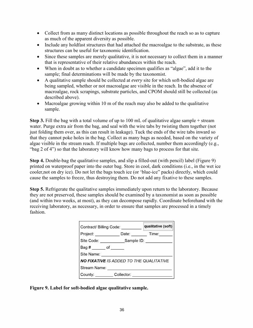
36
• Collect from as many distinct locations as possible throughout the reach so as to capture as much of the apparent diversity as possible.
• Include any holdfast structures that had attached the macroalgae to the substrate, as these structures can be useful for taxonomic identification.
• Since these samples are merely qualitative, it is not necessary to collect them in a manner that is representative of their relative abundances within the reach.
• When in doubt as to whether a candidate specimen qualifies as “algae”, add it to the sample; final determinations will be made by the taxonomist.
• A qualitative sample should be collected at every site for which soft-bodied algae are being sampled, whether or not macroalgae are visible in the reach. In the absence of macroalgae, rock scrapings, substrate particles, and CPOM should still be collected (as described above).
• Macroalgae growing within 10 m of the reach may also be added to the qualitative sample.
Step 3. Fill the bag with a total volume of up to 100 mL of qualitative algae sample + stream water. Purge extra air from the bag, and seal with the wire tabs by twisting them together (not just folding them over, as this can result in leakage). Tuck the ends of the wire tabs inward so that they cannot poke holes in the bag. Collect as many bags as needed, based on the variety of algae visible in the stream reach. If multiple bags are collected, number them accordingly (e.g., “bag 2 of 4”) so that the laboratory will know how many bags to process for that site. Step 4. Double-bag the qualitative samples, and slip a filled-out (with pencil) label (Figure 9) printed on waterproof paper into the outer bag. Store in cool, dark conditions (i.e., in the wet ice cooler,not on dry ice). Do not let the bags touch ice (or ‘blue-ice” packs) directly, which could cause the samples to freeze, thus destroying them. Do not add any fixative to these samples. Step 5. Refrigerate the qualitative samples immediately upon return to the laboratory. Because they are not preserved, these samples should be examined by a taxonomist as soon as possible (and within two weeks, at most), as they can decompose rapidly. Coordinate beforehand with the receiving laboratory, as necessary, in order to ensure that samples are processed in a timely fashion.
Figure 9. Label for soft-bodied algae qualitative sample.
37
5. BIOTIC SAMPLE PROCESSING
5.1 Module A (continued): Processing Benthic Macroinvertebrate Samples Step 1. Once all BMI subsamples (11 for RWB or MCM) have been collected and composited, transfer the composited sample to one or more 500-mL wide-mouth plastic sample jar, preferably one with straight edges. Never fill a jar more than halfway with sampled material; use as many jars as necessary in order to prevent this. Samples with a lot of organic material (e.g., plants, algae, leaf litter) tend to contain a lot of water that may inhibit sample preservation. Gently squeeze out as much water as possible (through the mesh of the D-frame net) before placing the sample in the jar, to prevent diluting the alcohol too much. Approach this task gingerly, so as not to damage invertebrates during this process. Invert the contents of the D-frame net into the sample jar. Perform this operation over a large, white tray to avoid loss of any sampled material and make recovery of spilled organisms easier. If possible, remove the larger twigs and rocks by hand after carefully inspecting for clinging organisms. Use forceps to remove any organisms clinging to the net and place these in the sample jar. All samples should be completely transferred to the sample jar without elutriation. If the samples contain a lot of fine particles, confirm that the sampling procedure is being executed correctly (i.e., use care to disturb the substrate as gently as possible and avoid kicking).17 Step 2. Place a date/locality label (Figure 10), filled out in pencil, on the inside of the jar and completely fill the jar with 95% ethanol18. To ensure proper preservation of BMIs, gently rotate jars that contain mostly mud or sand so that the ethanol is well distributed. Affix a second waterproof label on the outside of the jar. It is recommended that the label for the outside of the jar be printed with a laser printer (with alcohol-proof toner); otherwise, fill the label out by hand in pencil. Tape the label with transparent tape. Make sure all samples have both internal and external labels.
17 Samples with an abundance of sand or organic material should be processed expeditiously at the lab, as specimens in these samples can degrade quickly. Therefore, the presence of these kinds of samples should be communicated to the taxonomy lab as soon as possible and they should not be stored for a long time before delivering to the taxonomy lab for processing. See Woodard et al. 2012 for details 18 Note that the target concentration of ethanol is 70%, but 95% ethanol is used in the field to compensate for dilution from water in the sample. Final concentration of ethanol can be confirmed in the laboratory upon receipt of samples.
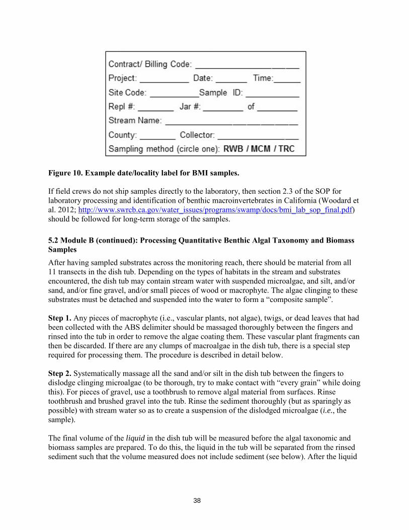
38
Figure 10. Example date/locality label for BMI samples. If field crews do not ship samples directly to the laboratory, then section 2.3 of the SOP for laboratory processing and identification of benthic macroinvertebrates in California (Woodard et al. 2012; http://www.swrcb.ca.gov/water_issues/programs/swamp/docs/bmi_lab_sop_final.pdf) should be followed for long-term storage of the samples. 5.2 Module B (continued): Processing Quantitative Benthic Algal Taxonomy and Biomass Samples After having sampled substrates across the monitoring reach, there should be material from all 11 transects in the dish tub. Depending on the types of habitats in the stream and substrates encountered, the dish tub may contain stream water with suspended microalgae, and silt, and/or sand, and/or fine gravel, and/or small pieces of wood or macrophyte. The algae clinging to these substrates must be detached and suspended into the water to form a “composite sample”. Step 1. Any pieces of macrophyte (i.e., vascular plants, not algae), twigs, or dead leaves that had been collected with the ABS delimiter should be massaged thoroughly between the fingers and rinsed into the tub in order to remove the algae coating them. These vascular plant fragments can then be discarded. If there are any clumps of macroalgae in the dish tub, there is a special step required for processing them. The procedure is described in detail below. Step 2. Systematically massage all the sand and/or silt in the dish tub between the fingers to dislodge clinging microalgae (to be thorough, try to make contact with “every grain” while doing this). For pieces of gravel, use a toothbrush to remove algal material from surfaces. Rinse toothbrush and brushed gravel into the tub. Rinse the sediment thoroughly (but as sparingly as possible) with stream water so as to create a suspension of the dislodged microalgae (i.e., the sample). The final volume of the liquid in the dish tub will be measured before the algal taxonomic and biomass samples are prepared. To do this, the liquid in the tub will be separated from the rinsed sediment such that the volume measured does not include sediment (see below). After the liquid
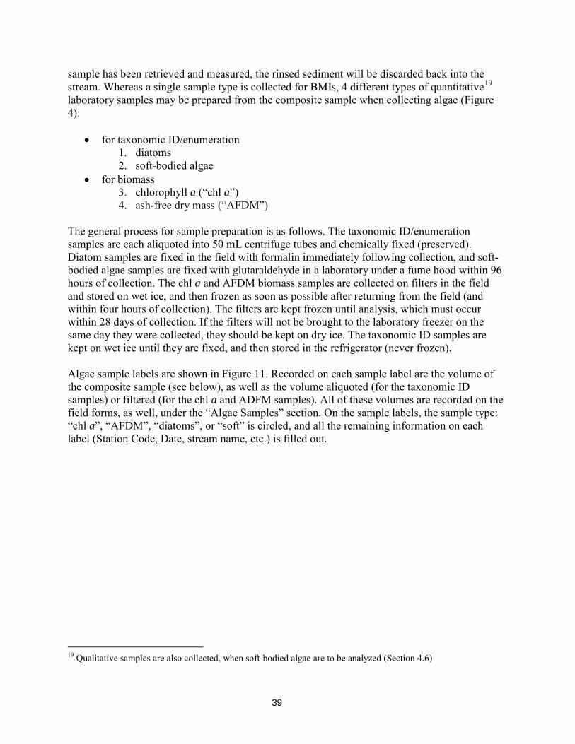
39
sample has been retrieved and measured, the rinsed sediment will be discarded back into the stream. Whereas a single sample type is collected for BMIs, 4 different types of quantitative19 laboratory samples may be prepared from the composite sample when collecting algae (Figure 4):
• for taxonomic ID/enumeration 1. diatoms 2. soft-bodied algae
• for biomass 3. chlorophyll a (“chl a”) 4. ash-free dry mass (“AFDM”)
The general process for sample preparation is as follows. The taxonomic ID/enumeration samples are each aliquoted into 50 mL centrifuge tubes and chemically fixed (preserved). Diatom samples are fixed in the field with formalin immediately following collection, and soft-bodied algae samples are fixed with glutaraldehyde in a laboratory under a fume hood within 96 hours of collection. The chl a and AFDM biomass samples are collected on filters in the field and stored on wet ice, and then frozen as soon as possible after returning from the field (and within four hours of collection). The filters are kept frozen until analysis, which must occur within 28 days of collection. If the filters will not be brought to the laboratory freezer on the same day they were collected, they should be kept on dry ice. The taxonomic ID samples are kept on wet ice until they are fixed, and then stored in the refrigerator (never frozen). Algae sample labels are shown in Figure 11. Recorded on each sample label are the volume of the composite sample (see below), as well as the volume aliquoted (for the taxonomic ID samples) or filtered (for the chl a and ADFM samples). All of these volumes are recorded on the field forms, as well, under the “Algae Samples” section. On the sample labels, the sample type: “chl a”, “AFDM”, “diatoms”, or “soft” is circled, and all the remaining information on each label (Station Code, Date, stream name, etc.) is filled out.
19 Qualitative samples are also collected, when soft-bodied algae are to be analyzed (Section 4.6)
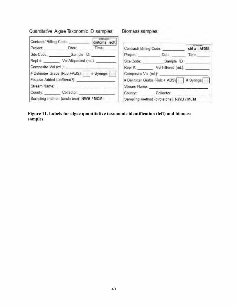
40
Figure 11. Labels for algae quantitative taxonomic identification (left) and biomass samples.
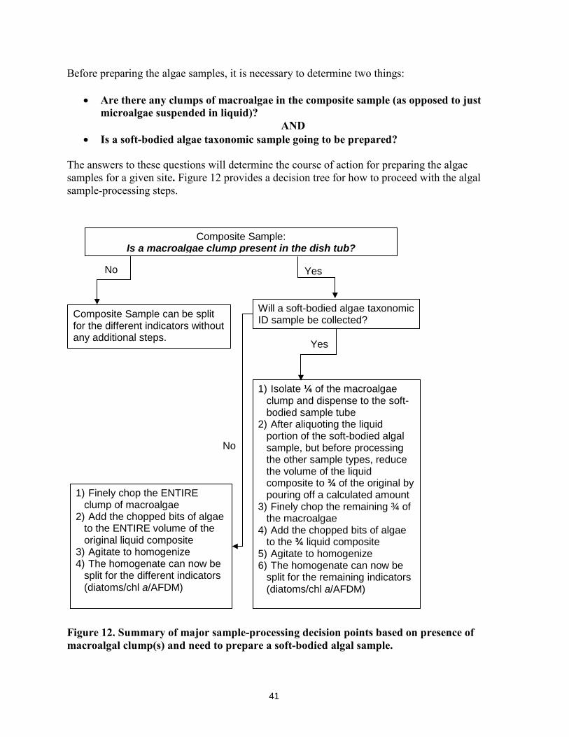
41
Before preparing the algae samples, it is necessary to determine two things:
• Are there any clumps of macroalgae in the composite sample (as opposed to just microalgae suspended in liquid)?
AND • Is a soft-bodied algae taxonomic sample going to be prepared?
The answers to these questions will determine the course of action for preparing the algae samples for a given site. Figure 12 provides a decision tree for how to proceed with the algal sample-processing steps.
Figure 12. Summary of major sample-processing decision points based on presence of macroalgal clump(s) and need to prepare a soft-bodied algal sample.
Composite Sample can be split for the different indicators without any additional steps.
Composite Sample: Is a macroalgae clump present in the dish tub?
Will a soft-bodied algae taxonomic ID sample be collected?
1) Finely chop the ENTIRE clump of macroalgae
2) Add the chopped bits of algae to the ENTIRE volume of the original liquid composite
3) Agitate to homogenize 4) The homogenate can now be
split for the different indicators (diatoms/chl a/AFDM)
1) Isolate ¼ of the macroalgae clump and dispense to the soft-bodied sample tube
2) After aliquoting the liquid portion of the soft-bodied algal sample, but before processing the other sample types, reduce the volume of the liquid composite to ¾ of the original by pouring off a calculated amount
3) Finely chop the remaining ¾ of the macroalgae
4) Add the chopped bits of algae to the ¾ liquid composite
5) Agitate to homogenize 6) The homogenate can now be
split for the remaining indicators (diatoms/chl a/AFDM)
No Yes
No
Yes
42
The following is a description of how to proceed when a soft-bodied algal taxonomic ID sample is to be prepared AND macroalgal clump(s) are present in the sample in the dish tub. A flowchart of this procedure is provided in Figure 13. It is recommended that this flowchart be printed in color, laminated (if possible) or printed on water-proof paper, and brought along to the field for a quick reference on handling macroalgal clumps in the composite sample. Note: It is unlikely that the ¼ macroalgal clump will occupy all the space in the soft-bodied algae quantitative sample tube, but if it does, a second tube will be needed in order to accommodate all the sample material plus liquid. If such an action is taken, it should be noted in the Comments section of the field sheets and the tubes should be clearly identified as belonging to the same sample, for record-keeping purposes. Do not fill either tube so full that there will not be enough room for the fixative.

43
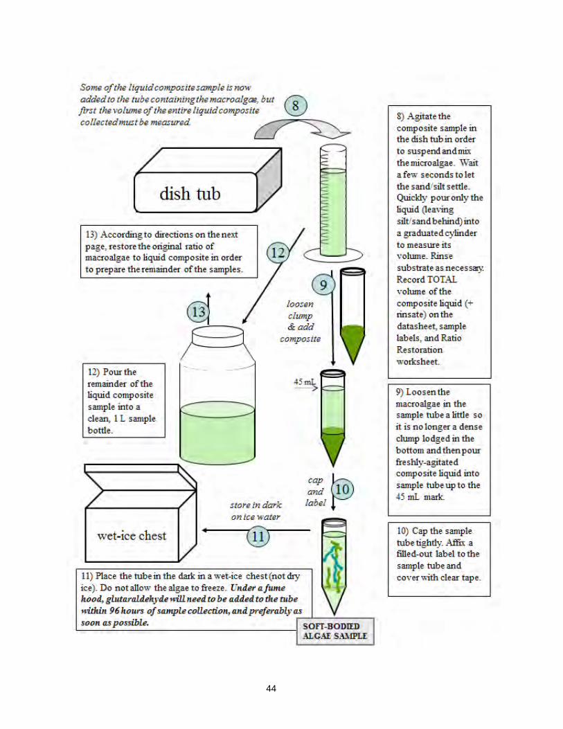
44
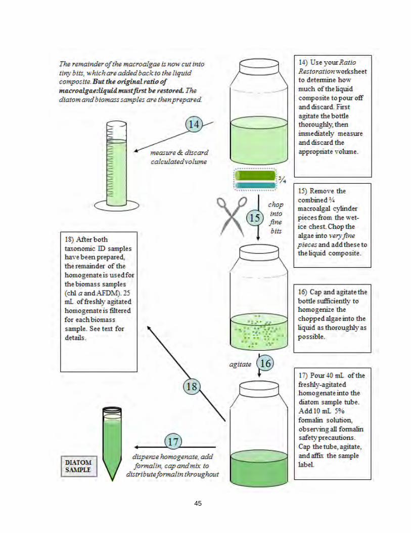
45
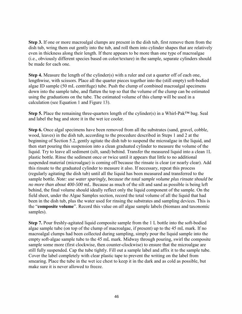
46
Step 3. If one or more macroalgal clumps are present in the dish tub, first remove them from the dish tub, wring them out gently into the tub, and roll them into cylinder shapes that are relatively even in thickness along their length. If there appears to be more than one type of macroalgae (i.e., obviously different species based on color/texture) in the sample, separate cylinders should be made for each one. Step 4. Measure the length of the cylinder(s) with a ruler and cut a quarter off of each one, lengthwise, with scissors. Place all the quarter pieces together into the (still empty) soft-bodied algae ID sample (50 mL centrifuge) tube. Push the clump of combined macroalgal specimens down into the sample tube, and flatten the top so that the volume of the clump can be estimated using the graduations on the tube. The estimated volume of this clump will be used in a calculation (see Equation 1 and Figure 13). Step 5. Place the remaining three-quarters length of the cylinder(s) in a Whirl-Pak™ bag. Seal and label the bag and store it in the wet ice cooler. Step 6. Once algal specimens have been removed from all the substrates (sand, gravel, cobble, wood, leaves) in the dish tub, according to the procedure described in Steps 1 and 2 at the beginning of Section 5.2, gently agitate the dish tub to suspend the microalgae in the liquid, and then start pouring this suspension into a clean graduated cylinder to measure the volume of the liquid. Try to leave all sediment (silt, sand) behind. Transfer the measured liquid into a clean 1L plastic bottle. Rinse the sediment once or twice until it appears that little to no additional suspended material (microalgae) is coming off because the rinsate is clear (or nearly clear). Add this rinsate to the graduated cylinder to measure it also. If necessary, repeat this process (regularly agitating the dish tub) until all the liquid has been measured and transferred to the sample bottle. Note: use water sparingly, because the total sample volume plus rinsate should be no more than about 400-500 mL. Because as much of the silt and sand as possible is being left behind, the final volume should ideally reflect only the liquid component of the sample. On the field sheet, under the Algae Samples section, record the total volume of all the liquid that had been in the dish tub, plus the water used for rinsing the substrates and sampling devices. This is the “composite volume”. Record this value on all algae sample labels (biomass and taxonomic samples). Step 7. Pour freshly-agitated liquid composite sample from the 1 L bottle into the soft-bodied algae sample tube (on top of the clump of macroalgae, if present) up to the 45 mL mark. If no macroalgal clumps had been collected during sampling, simply pour the liquid sample into the empty soft-algae sample tube to the 45 mL mark. Midway through pouring, swirl the composite sample some more (first clockwise, then counter-clockwise) to ensure that the microalgae are still fully suspended. Cap the tube tightly. Fill out a sample label and affix it to the sample tube. Cover the label completely with clear plastic tape to prevent the writing on the label from smearing. Place the tube in the wet ice chest to keep it in the dark and as cold as possible, but make sure it is never allowed to freeze.

47
Glutaraldehyde is necessary for fixing soft-bodied algae samples in order to preserve fine morphological features and pigment colors, as both can be crucial characters for taxonomic determination. However, glutaraldehyde is a hazardous substance that poses a number of safety risks. As such, it must be handled only in a fume hood, by trained personnel wearing appropriate protective gear. Refer to the Guidance Document for an SOP on handling glutaraldehyde. To fix the soft-bodied algae sample: working under a fume hood, add glutaraldehyde to the tube to a final concentration of 2%. This can be achieved, for example, by adding 5 mL of 20% glutaraldehyde to 45 mL of sample. Distribute the glutaraldehyde throughout the sample by inverting the tightly closed tube repeatedly. Once the samples are fixed, they must be stored in the dark in a refrigerator. Wrap the tubes in foil, if necessary, to maintain darkness. If no fume hood is available, arrangements should be made for the glutaraldehyde to be added to the samples by personnel with access to a hood (e.g., the taxonomy lab). In the meantime, the unfixed samples must be kept in the dark and on wet ice (but not allowed to freeze), and must be fixed within 96 hours of collection (and preferably sooner). Therefore, if the taxonomy laboratory or another party will be adding the fixative, it is imperative to plan ahead to arrange for this to be done in a timely manner, and also to clearly mark which tubes will need to have fixative added to them. Step 8. In the field, after the (unfixed) soft-bodied algal sample has been prepared, and before preparing the diatom sample (and biomass samples, which will be discussed in the next steps), if a macroalgal clump had been present in the dish tub, then the volume of the remaining composite liquid must be reduced to equal ¾ of the original volume. This is necessary because ¼ of the macroalgal clump was taken out of the composite sample but a full ¼ was not removed from the liquid portion. As such, the original ratio between liquid and macroalgae must be restored before further sample preparation. The following procedure is used to reduce the volume of liquid composite to ¾ of the original. For convenience, the following formula (Equation 1) can be used to calculate how many mL to pour off and discard from the composite:
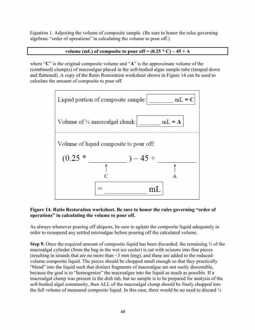
48
Equation 1. Adjusting the volume of composite sample. (Be sure to honor the rules governing algebraic “order of operations” in calculating the volume to pour off.)
volume (mL) of composite to pour off = (0.25 * C) – 45 + A where “C” is the original composite volume and “A” is the approximate volume of the (combined) clump(s) of macroalgae placed in the soft-bodied algae sample tube (tamped down and flattened). A copy of the Ratio Restoration worksheet shown in Figure 14 can be used to calculate the amount of composite to pour off.
Figure 14. Ratio Restoration worksheet. Be sure to honor the rules governing “order of operations” in calculating the volume to pour off. As always whenever pouring off aliquots, be sure to agitate the composite liquid adequately in order to resuspend any settled microalgae before pouring off the calculated volume. Step 9. Once the required amount of composite liquid has been discarded, the remaining ¾ of the macroalgal cylinder (from the bag in the wet ice cooler) is cut with scissors into fine pieces (resulting in strands that are no more than ~3 mm long), and these are added to the reduced-volume composite liquid. The pieces should be chopped small enough so that they practically “blend” into the liquid such that distinct fragments of macroalgae are not easily discernible, because the goal is to “homogenize” the macroalgae into the liquid as much as possible. If a macroalgal clump was present in the dish tub, but no sample is to be prepared for analysis of the soft-bodied algal community, then ALL of the macroalgal clump should be finely chopped into the full volume of measured composite liquid. In this case, there would be no need to discard ¼
49
of the composite volume before introducing the (full amount of) chopped macroalgal into the liquid. Step 10. After introducing the finely chopped macroalgae into the composite liquid, cap the composite bottle and agitate sufficiently to homogenize the tiny bits of algae into the liquid as much as possible, while not agitating so hard as to risk busting cells and releasing chl a. Step 11. To prepare the diatom sample, aliquot 40 mL of freshly-agitated sample homogenate into the diatom ID sample tube, swirling the composite sample bottle again midway through pouring to keep the algae suspended. Add 10 mL of the 5% formalin to the sample (for a final concentration of 1%). Fixatives such as formalin must be used with great care. Be sure to wear formalin-safe gloves and safety goggles when using the fixative, as it should never be touched with bare hands or allowed to splash onto skin or into eyes. Also make sure it is used only in a very well-ventilated place and avoid breathing in any fumes. Minimize the amount of time that vessels containing formalin are open. Fixative added to the sample must not be allowed to ooze outside the vessel that contains it, including the sample tubes. Refer to the Guidance Document for instructions on preparing the buffered formalin solution and for an SOP on handling formalin. Step 12. Cap the tube tightly and invert it several times to mix the formalin into the sample. Fill out a sample label and affix it to the sample tube. Cover the label completely with clear plastic tape to prevent the writing on the label from smearing. Keep the fixed diatom samples in the dark and away from heat. The remaining composite sample homogenate can be used to prepare the chl-a and AFDM filters as described below. If no algal taxonomic data are required for the project at hand, and only biomass data are needed, finely chop all macroalgae (if present) directly into the entire volume of liquid (which must still be measured and recorded). Then proceed to Step 13. Step 13. Now the biomass samples can be prepared. The procedure to filter chl a samples should be carried out quickly, and in the shade as much as possible, to minimize exposure of the sample to light/heat, thus minimizing chl a degradation. Use clean filter forceps to center a glass fiber filter (47 mm, 0.7 µm pore size) onto the mesh platform of a clean filtering apparatus, and rinse the filter a little with DI water to seat it well into the mesh before attaching the filter chamber on top. Never touch the filters with hands or anything other than clean forceps. Agitate the sample homogenate to resuspend all the macroalgal fragments and microalgal material. Measure 25 mL using a small, clean graduated cylinder. Midway through pouring the 25 mL, swirl the homogenate again to ensure that the material is still fully suspended. Pour the remainder of the 25 mL into the filter chamber. Once empty, rinse the graduated cylinder with a few mL of DI water, and add this to the filter chamber. Step 14. To filter the sample, create a gentle vacuum with the hand pump. Be sure to proceed very slowly, and pump only one stroke at a time until all of the liquid in the sample is passed through the filter. Pressure on the sample should never exceed 7 psi, as this could cause cells to burst and release contents, including chl a, into the filtrate and be lost. If it becomes impossible to filter a whole 25 mL of the sample and remove the water efficiently, discard the filter and try
50
again with a smaller volume (e.g., 10 mL). It is not necessary to collect on multiple filters to try to achieve a total volume of 25 mL. Simply filter as much as possible on a single filter, up to 25 mL, and then use that filter as the sample. Be sure to record the volume of the composite sample that was actually filtered, both on the datasheet, and on the sample label. Rinse the sides of the filter chamber with a few mL of DI water, and continue filtering until the water is drawn down. The filter should not be sucked dry, but rather left slightly moist, in order to avoid applying excessive pressure to the sample, which could cause algal cells to burst. After all the liquid has passed through, check the filter to see if there are any bits of non-algal plant matter (like tiny seedlings or bits of leaves). If so, remove them with clean, pointed forceps, being careful not to remove any algae in the process. Remove the filter from the filtering device. Always thoroughly rinse the sides of the filter chamber and the interface between the mesh filter seating and the screw-on part of the apparatus with DI water between samples. Step 15. Fold the filter in half (with the sample material on the inside, like a taco) using the forceps, and place it inside a clean, snap-top Petri dish. Envelope the Petri dish completely within a small sheet of aluminum foil in order to prevent any light from reaching the filter. Place the covered Petri dish and its corresponding, filled-out sample label (face outward) into a 100 mL Whirl-Pak™ bag, purge as much of the air out of the bag as possible, “whirl” it shut, and seal it tightly by twisting its wire tabs together, so that water in the cooler will not be able to enter the bag. Shove the sample packet down into the ice in the cooler to make sure it stays submerged and does not float to the top. This may be achieved by sealing the sample bags in a large Ziploc™ bag with a rock in it. Keep chlorophyll a filters as cold as possible and place them in the freezer (-80º, if available) or on dry ice as soon as possible (and within four hours of collection); the analytical holding time for the chl a filters is 28 days from collection, when kept frozen. Step 16. For the AFDM samples, use glass-fiber filters (47 mm, 0.7 µm pore size) that have been pre-combusted20. Never touch the filters with hands or anything other than clean forceps. Follow the same process as that used for chl-a sample filtering. Record the volume filtered for the AFDM sample. Keep AFDM filters as cold as possible until the samples can be frozen back at the laboratory that evening, or place on dry ice until they can be stored in the laboratory freezer. The analytical holding time for the AFDM samples is 28 days from collection, when kept frozen.
20 Check with the laboratory that will be analyzing the samples about obtaining pre-combusted filters.
51
6. PHYSICAL HABITAT TRANSECT-BASED MEASUREMENTS
After all biotic samples have been collected at a given transect, PHab data collection may begin. These data are designed to characterize a stream reach’s physical habitat, knowledge about which can aid interpretation of the biotic data. In some cases, however, PHab data may be desired for a site assessment even when biotic/biomass samples are not being collected. The majority of PHab measurements in this SOP are gathered relative to the 11 main transects (Figure 3), and data for the PHab parameters described in this section are entered on transect-specific field sheets (and in the case of the “Pebble Count” data, also on the inter-transect field sheets). PHab data collection starts at the downstream transect (Transect A) and proceeds working upstream along the monitoring reach. Some programs (e.g., citizen monitoring efforts) may elect to collect a less-intensive subset of PHab data than the full suite described here. To this end, the Guidance Document provides suggestions for a “Basic” protocol. 6.1 Module C: Wetted Width and Bankfull Dimensions Step 1. Measure the wetted width associated with the transect and record this (in meters) in the box at the top of the transect form. The wetted channel is the zone that is inundated with water and the wetted width is the distance between the sides of the channel at the point where substrates are no longer surrounded by surface water (Figure 15). The wetted width can include emergent, unvegetated sandbars or boulders in the middle of a channel, but should not include emergent, vegetated “islands” (defined as features that are not flooded during average year high-water events). When a transect crosses an island, subtract the width of the island from the distance between the wetted margins. Step 2. Scout beyond the wetted channel along the stream reach to identify the location of the bankfull margins on either bank by looking for evidence of annual or semi-annual flood events. The bankfull channel is the zone of maximum water inundation in a normal-flow year (i.e., one- to two-year flood events; see Figure 15 and the Guidance Document for a depiction of wetted width and bankfull dimensions). Because most channel-formation processes are believed to act when flows are within this zone (Mount 1995), bankfull dimensions provide a valuable indication of stream power during high-flow events and therefore relative size of the water body. Examples of evidence for bankfull location include topographic, vegetation, and geologic cues (changes in bank slope, changes from annual to perennial vegetation, changes in the size distribution of surface sediments, location of water stains on concrete and bedrock channels, etc.). Although it is tempting to use the position of drift material caught in vegetation to identify bankfull location, it only indicates the discharge height during extreme recent flow events, and should not be used as an indicator by itself. Note that, perhaps more than any other component of PHab assessment, identification of bankfull location requires extensive experience in multiple ecoregions and stream types, and training in the field under the supervision of experienced bioassessment practitioners is essential.
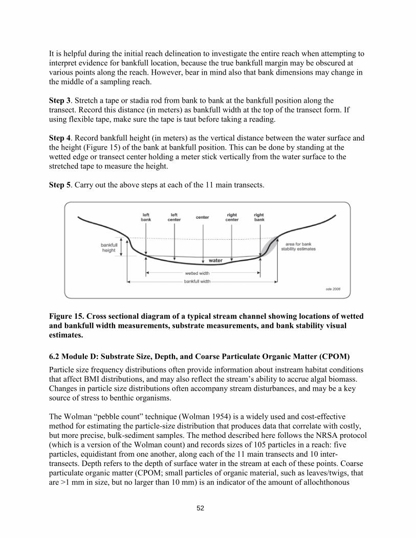
52
It is helpful during the initial reach delineation to investigate the entire reach when attempting to interpret evidence for bankfull location, because the true bankfull margin may be obscured at various points along the reach. However, bear in mind also that bank dimensions may change in the middle of a sampling reach. Step 3. Stretch a tape or stadia rod from bank to bank at the bankfull position along the transect. Record this distance (in meters) as bankfull width at the top of the transect form. If using flexible tape, make sure the tape is taut before taking a reading. Step 4. Record bankfull height (in meters) as the vertical distance between the water surface and the height (Figure 15) of the bank at bankfull position. This can be done by standing at the wetted edge or transect center holding a meter stick vertically from the water surface to the stretched tape to measure the height. Step 5. Carry out the above steps at each of the 11 main transects.
Figure 15. Cross sectional diagram of a typical stream channel showing locations of wetted and bankfull width measurements, substrate measurements, and bank stability visual estimates. 6.2 Module D: Substrate Size, Depth, and Coarse Particulate Organic Matter (CPOM) Particle size frequency distributions often provide information about instream habitat conditions that affect BMI distributions, and may also reflect the stream’s ability to accrue algal biomass. Changes in particle size distributions often accompany stream disturbances, and may be a key source of stress to benthic organisms. The Wolman “pebble count” technique (Wolman 1954) is a widely used and cost-effective method for estimating the particle-size distribution that produces data that correlate with costly, but more precise, bulk-sediment samples. The method described here follows the NRSA protocol (which is a version of the Wolman count) and records sizes of 105 particles in a reach: five particles, equidistant from one another, along each of the 11 main transects and 10 inter-transects. Depth refers to the depth of surface water in the stream at each of these points. Coarse particulate organic matter (CPOM; small particles of organic material, such as leaves/twigs, that are >1 mm in size, but no larger than 10 mm) is an indicator of the amount of allochthonous
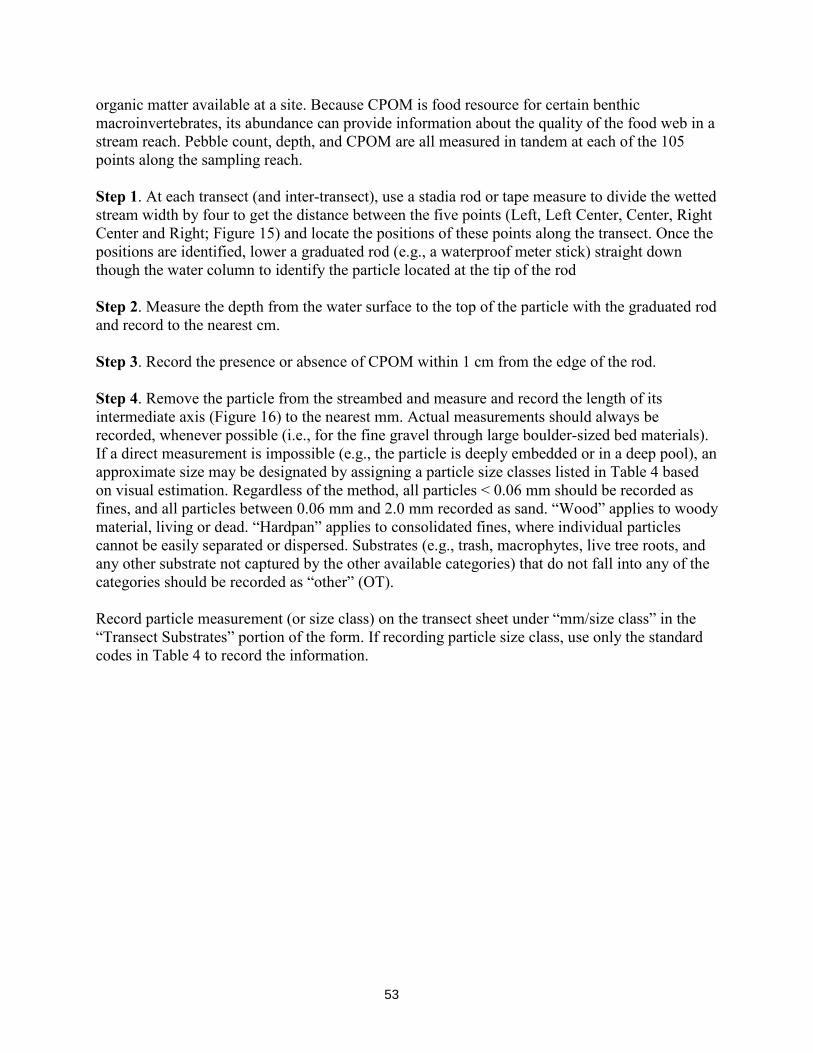
53
organic matter available at a site. Because CPOM is food resource for certain benthic macroinvertebrates, its abundance can provide information about the quality of the food web in a stream reach. Pebble count, depth, and CPOM are all measured in tandem at each of the 105 points along the sampling reach. Step 1. At each transect (and inter-transect), use a stadia rod or tape measure to divide the wetted stream width by four to get the distance between the five points (Left, Left Center, Center, Right Center and Right; Figure 15) and locate the positions of these points along the transect. Once the positions are identified, lower a graduated rod (e.g., a waterproof meter stick) straight down though the water column to identify the particle located at the tip of the rod Step 2. Measure the depth from the water surface to the top of the particle with the graduated rod and record to the nearest cm. Step 3. Record the presence or absence of CPOM within 1 cm from the edge of the rod. Step 4. Remove the particle from the streambed and measure and record the length of its intermediate axis (Figure 16) to the nearest mm. Actual measurements should always be recorded, whenever possible (i.e., for the fine gravel through large boulder-sized bed materials). If a direct measurement is impossible (e.g., the particle is deeply embedded or in a deep pool), an approximate size may be designated by assigning a particle size classes listed in Table 4 based on visual estimation. Regardless of the method, all particles < 0.06 mm should be recorded as fines, and all particles between 0.06 mm and 2.0 mm recorded as sand. “Wood” applies to woody material, living or dead. “Hardpan” applies to consolidated fines, where individual particles cannot be easily separated or dispersed. Substrates (e.g., trash, macrophytes, live tree roots, and any other substrate not captured by the other available categories) that do not fall into any of the categories should be recorded as “other” (OT). Record particle measurement (or size class) on the transect sheet under “mm/size class” in the “Transect Substrates” portion of the form. If recording particle size class, use only the standard codes in Table 4 to record the information.
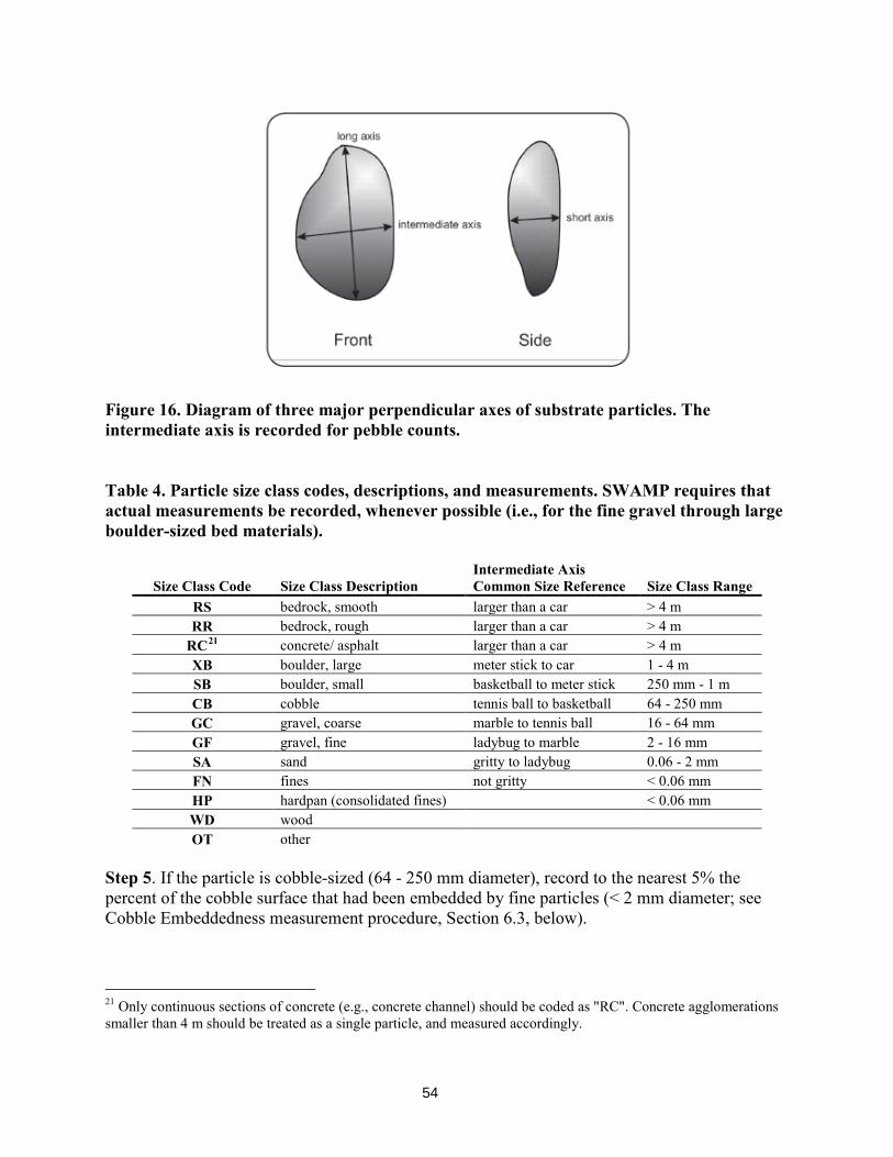
54
Figure 16. Diagram of three major perpendicular axes of substrate particles. The intermediate axis is recorded for pebble counts. Table 4. Particle size class codes, descriptions, and measurements. SWAMP requires that actual measurements be recorded, whenever possible (i.e., for the fine gravel through large boulder-sized bed materials).
Size Class Code Size Class Description Intermediate Axis Common Size Reference Size Class Range
RS bedrock, smooth larger than a car > 4 m RR bedrock, rough larger than a car > 4 m
RC21 concrete/ asphalt larger than a car > 4 m XB boulder, large meter stick to car 1 - 4 m SB boulder, small basketball to meter stick 250 mm - 1 m CB cobble tennis ball to basketball 64 - 250 mm GC gravel, coarse marble to tennis ball 16 - 64 mm GF gravel, fine ladybug to marble 2 - 16 mm SA sand gritty to ladybug 0.06 - 2 mm FN fines not gritty < 0.06 mm HP hardpan (consolidated fines) < 0.06 mm WD wood OT other
Step 5. If the particle is cobble-sized (64 - 250 mm diameter), record to the nearest 5% the percent of the cobble surface that had been embedded by fine particles (< 2 mm diameter; see Cobble Embeddedness measurement procedure, Section 6.3, below).
21 Only continuous sections of concrete (e.g., concrete channel) should be coded as "RC". Concrete agglomerations smaller than 4 m should be treated as a single particle, and measured accordingly.
55
Sometimes points with dry (not submerged or moist) substrates are encountered during the course of PHab data collection along transects/inter-transects. To determine how to collect data at dry sampling points, it is necessary to first establish whether the dry area in question lies within the stream’s active channel (i.e., therefore regularly inundated during storms), or whether the point is on a stable island (i.e., therefore rarely, if ever, inundated). Stable islands are typically vegetated, often with woody shrubs or trees, and have heights near or exceeding bankfull height. Pebble counts should not be conducted on stable islands. If the transect spans a portion of the study reach in which the channel is bifurcated such that there are two channels with an intervening island, the entire transect should be placed across the dominant channel, and all five pebble count points should be located on that side. If the point falls on a dry surface that is within the usual active channel (i.e., subject to regular disturbance by flows), then pebble count and primary-producer cover data from the dry point should be recorded as follows:
• score Depth as 0 • score Particle Size/Class and Embeddedness as described above for wet particles • score all the algae variables (Microalgae, Macroalgae Attached, and Macroalgae
Unattached), as well as Macrophytes and CPOM, as “D” for “dry”
Ordinarily, the sampling transect would span the wetted width of the channel, but when no water is present at a given transect, evidence of the typical wetted extent of the active channel will need to be used to infer appropriate transect boundaries. Such indicators can include the transition from vegetated to unvegetated area (i.e., moving from banks toward the active channel), as well as the presence of dried algae, water stains, micro-topographic transitions, changes in substrate composition, soil cracks, and others. 6.3 Module E: Cobble Embeddedness The degree to which fine particles fill interstitial spaces in the streambed has a significant impact on the ecology of benthic organisms and fish, but techniques for measuring this impact vary greatly (this is summarized by Sylte and Fischenich 2002, http://stream.fs.fed.us/news/streamnt/pdf/StreamOCT4.pdf ). Here we define embeddedness as the percent of the surface area (not volume) of cobble-sized particles (64 - 250 mm) that is buried by fines or sand particles (< 2.0 mm diameter). Ideally, at least 25 cobbles are assessed for embeddedness in each sampling reach: Embeddedness is determined for each cobble that is measured for particle size, up to a total of 25 cobbles. If < 25 cobbles are encountered during the pebble count, the remainder are “made up” by assessing cobbles that lie outside of the PHab data collection transects (see Step 3, below). In certain streams, it may not be possible to find 25 cobbles. Step 1. Every time a cobble-sized particle is encountered during the pebble count, remove the cobble from the stream bed and visually estimate the percentage of the cobble’s surface area that had been buried by fine particles. If removal of the cobble is impossible, approximate embeddedness to the best extent possible. In the rare circumstances that multiple sample points
56
land on the same cobble, do not take a second embeddedness measurement. Once embeddedness has been assessed for 25 cobbles, no more need be assessed. Step 2. Record the embeddedness values for the first 25 cobble-sized particles encountered during the pebble count in the “% Cobble Embed” field in the “Transect Substrates” portion of the transect sheet. Step 3. If 25 cobbles are not encountered during the pebble count by the time Transect K has been sampled, supplement the data by conducting a “random walk” 22. Starting at a random point in the reach, follow a line from one bank to the other at a randomly chosen angle, recording embeddedness of any cobbles encountered (that were not previously recorded) along the way. Upon arriving at the other bank, reverse the process with a new randomly chosen angle. Spend a maximum of 10 minutes on the random walk, even if 25 cobbles have not been encountered by that time. Embeddedness for any cobbles encountered outside of the pebble count locations should be recorded in the “Additional Cobble Embeddedness” section of the field sheets.23 6.4 Module F: Algal and Macrophyte Cover Algal cover refers to the amount of algae in the stream reach, both in terms of 1) microalgal coatings (“slimy-ness”) on stream substrates and 2) macroalgae (e.g., filaments, mats, globules)24. It is a reflection of stream primary production and has implications for the health of food webs as well as the damaging effects of eutrophication stimulated by excess nutrients in concert with other environmental co-factors (e.g., loss of canopy cover). Algal cover is estimated by a point-intercept approach that entails collecting information about the presence/absence of both types of algae (as well as thickness, for the microalgae) at each of the 5 points along the transects associated with the pebble count. If the point corresponding to each pebble in the pebble count intercepts algae, then algae is recorded as “present” at that point. Step 1. For each point along the pebble count, record information about algae as follows. For any film-like coating of algae (referred to as “Microalgae” on the datasheet) present on the surface of the substrate at that point, estimate the presence / thickness category according to the scheme in Table 4. For thicker microalgal layers, a small ruler can be used for measurement. For layers too thin to measure, use the indicators listed in the last column of Table 4. Note that these thickness codes refer only to microalgal film, not macroalgal mats (macroalgal thickness is not assessed in this protocol).
22 It is preferable to wait until the rest of the PHab transect/inter-transect measures are complete before doing this, so as not to trample any as-yet unsampled transects in the course of the random walk. 23 An easy way to ensure that 25 embeddedness measurements are taken is to put an X in one of the boxes on the first data sheet each time a cobble is encountered during normal transect measurements. Then, after all transects are complete, fill in the remaining boxes with embeddedness estimates. 24 Refer to the glossary for comprehensive definitions of microalgae and macroalgae and the Guidance Document for photos
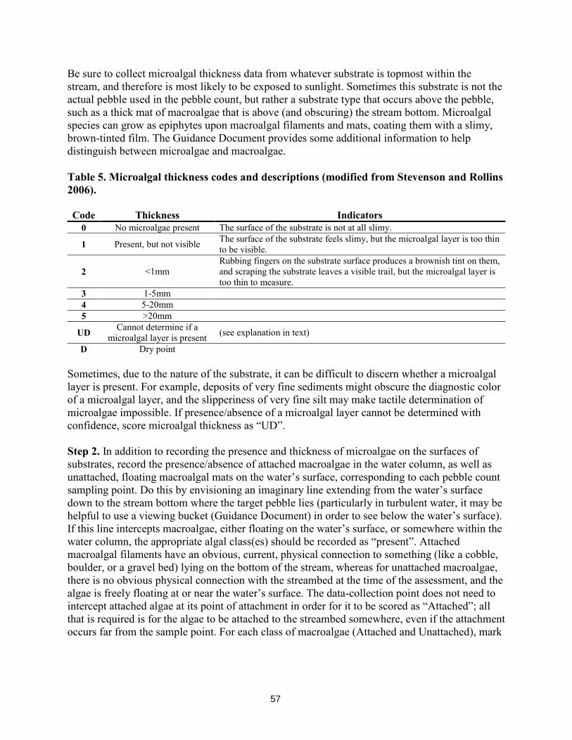
57
Be sure to collect microalgal thickness data from whatever substrate is topmost within the stream, and therefore is most likely to be exposed to sunlight. Sometimes this substrate is not the actual pebble used in the pebble count, but rather a substrate type that occurs above the pebble, such as a thick mat of macroalgae that is above (and obscuring) the stream bottom. Microalgal species can grow as epiphytes upon macroalgal filaments and mats, coating them with a slimy, brown-tinted film. The Guidance Document provides some additional information to help distinguish between microalgae and macroalgae. Table 5. Microalgal thickness codes and descriptions (modified from Stevenson and Rollins 2006). Code Thickness Indicators
0 No microalgae present The surface of the substrate is not at all slimy.
1 Present, but not visible The surface of the substrate feels slimy, but the microalgal layer is too thin to be visible.
2 <1mm Rubbing fingers on the substrate surface produces a brownish tint on them, and scraping the substrate leaves a visible trail, but the microalgal layer is too thin to measure.
3 1-5mm 4 5-20mm 5 >20mm
UD Cannot determine if a microalgal layer is present (see explanation in text)
D Dry point Sometimes, due to the nature of the substrate, it can be difficult to discern whether a microalgal layer is present. For example, deposits of very fine sediments might obscure the diagnostic color of a microalgal layer, and the slipperiness of very fine silt may make tactile determination of microalgae impossible. If presence/absence of a microalgal layer cannot be determined with confidence, score microalgal thickness as “UD”. Step 2. In addition to recording the presence and thickness of microalgae on the surfaces of substrates, record the presence/absence of attached macroalgae in the water column, as well as unattached, floating macroalgal mats on the water’s surface, corresponding to each pebble count sampling point. Do this by envisioning an imaginary line extending from the water’s surface down to the stream bottom where the target pebble lies (particularly in turbulent water, it may be helpful to use a viewing bucket (Guidance Document) in order to see below the water’s surface). If this line intercepts macroalgae, either floating on the water’s surface, or somewhere within the water column, the appropriate algal class(es) should be recorded as “present”. Attached macroalgal filaments have an obvious, current, physical connection to something (like a cobble, boulder, or a gravel bed) lying on the bottom of the stream, whereas for unattached macroalgae, there is no obvious physical connection with the streambed at the time of the assessment, and the algae is freely floating at or near the water’s surface. The data-collection point does not need to intercept attached algae at its point of attachment in order for it to be scored as “Attached”; all that is required is for the algae to be attached to the streambed somewhere, even if the attachment occurs far from the sample point. For each class of macroalgae (Attached and Unattached), mark
58
“P” (for “present”) if intercepted by the sampling point and “A” (for “absent”) if not intercepted.25 If any portion (above- or underwater) of a macrophyte is intercepted by the imaginary line associated with the pebble count point, mark “P” for “present” under “Macrophytes”. Otherwise, mark “A” for absent. Macrophytes are defined as herbaceous, vascular plants rooted or floating within the stream’s wetted channel, such as sedge, cattail, knotweed, Arundo donax, watercress, water-primrose, duckweed, etc. Our definition of aquatic macrophytes excludes trees, root mats, shrubs, mosses, and algae. This is the same as the definition of macrophytes used for Module J (Instream Habitat Complexity). 6.5 Module G: Bank Stability The vulnerability of stream banks to erosion is often of interest in bioassessment because of its direct relationship with sedimentation. For each transect, record a visual assessment of bank vulnerability along an imaginary line between the wetted width and bankfull width of the stream channel (Figure 15)26. Choose one of three vulnerability states: eroded (evidence of mass wasting), vulnerable (unprotected banks), or stable. All three states may be evident in a single reach at both natural and highly modified streams. The following indicators help describe the states: • Eroded: Exposed tree roots, obvious bank slumps, fallen trees. • Vulnerable: Sparse vegetation • Stable: Bank armoring, robust vegetation, few exposed tree roots 6.6 Module H: Human Influence The influence of human activities on stream biota is a central question in bioassessment analyses. Quantification of human activities is used to evaluate stress and to identify minimally disturbed reference sites. Reach-scale observations provide a crucial supplement to data provided by aerial imagery and GIS analysis. Anthropogenic features and activities associated with each main transect (for a distance of 5 m upstream and 5 m downstream from the transect, totaling a width of 10 m centered on the transect; Figure 17) are recorded in terms of zones based on how close they are to the wetted margins.27 The area in which human influence is measured extends outward 50 m in both directions from the bank along the entire reach.
25 Because pebble counts span the “wetted width” of each transect, pebbles at the margin positions will often be at least moist, and sometimes even submerged. As such, it is important to realize that algal cover can occur at the bank positions of the pebble count as well as intermediate positions across the stream. Algal cover should therefore be recorded at all five observation points along each transect. 26 Note that sandbars are not considered part of the bank. 27 The relative distance between the wetted and bankfull margins can complicate the assessment of human influence. If the wetted edge and the bankfull margin are at the same point, then land uses between the wetted edge and bankfull margin are not present, and that location cannot be scored. Conversely, in some streams, the bank and the wetted edge may be many meters apart. In that situation, the wetted edge should be used as a consistent point for defining the area.
59
For each human disturbance feature/activity class, circle “Y” if it is present between the wetted margins; otherwise, circle “N”, and then assess each side of the stream as follows: If the feature/activity is present between the wetted edge and bankfull margin, circle “B”; if it is outside within 10 m of the bank circle “C”; if it is within 50 m of the bank, circle “P”; otherwise, circle 0. The relative distance between the wetted and bankfull margins can If the wetted edge and the bankfull margin are at the same point, then land uses between the wetted edge and bankfull margin are not present, and that location cannot be scored. Conversely, in some streams, the bank and the wetted edge may be many meters apart. In that situation, the wetted edge should be used as a consistent point for defining the area. For each feature/activity, the most proximal category takes precedence and therefore is the distance at which that feature/activity should be scored. For example, if a feature/activity is observed within the channel, as well as on the banks, circle “Y” to denote the channel, and move on to scoring the next feature/activity class. Note that certain features (e.g., parks) are not applicable within the channel, and for these, “B” would represent the most proximal location possible. Table 6 provides definitions of Human Influence features/activities. Circle only the closest location for each impact that applies, being careful not to double-count any human influence observations. 28
28 Double counts are prevented by SWAMP electronic forms.
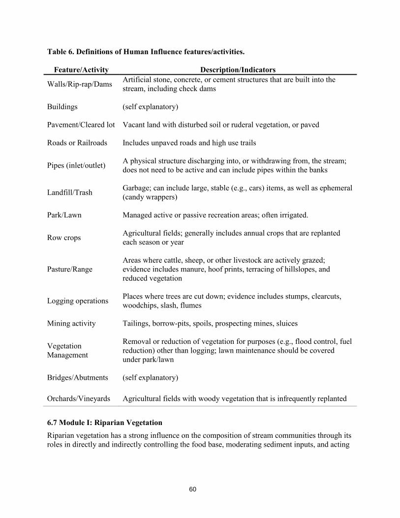
60
Table 6. Definitions of Human Influence features/activities.
Feature/Activity Description/Indicators
Walls/Rip-rap/Dams Artificial stone, concrete, or cement structures that are built into the stream, including check dams
Buildings (self explanatory) Pavement/Cleared lot Vacant land with disturbed soil or ruderal vegetation, or paved Roads or Railroads Includes unpaved roads and high use trails
Pipes (inlet/outlet)
A physical structure discharging into, or withdrawing from, the stream; does not need to be active and can include pipes within the banks
Landfill/Trash Garbage; can include large, stable (e.g., cars) items, as well as ephemeral (candy wrappers)
Park/Lawn Managed active or passive recreation areas; often irrigated.
Row crops Agricultural fields; generally includes annual crops that are replanted each season or year
Pasture/Range Areas where cattle, sheep, or other livestock are actively grazed; evidence includes manure, hoof prints, terracing of hillslopes, and reduced vegetation
Logging operations Places where trees are cut down; evidence includes stumps, clearcuts, woodchips, slash, flumes
Mining activity Tailings, borrow-pits, spoils, prospecting mines, sluices
Vegetation Management
Removal or reduction of vegetation for purposes (e.g., flood control, fuel reduction) other than logging; lawn maintenance should be covered under park/lawn
Bridges/Abutments (self explanatory) Orchards/Vineyards Agricultural fields with woody vegetation that is infrequently replanted 6.7 Module I: Riparian Vegetation Riparian vegetation has a strong influence on the composition of stream communities through its roles in directly and indirectly controlling the food base, moderating sediment inputs, and acting
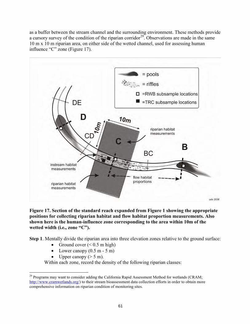
61
as a buffer between the stream channel and the surrounding environment. These methods provide a cursory survey of the condition of the riparian corridor29. Observations are made in the same 10 m x 10 m riparian area, on either side of the wetted channel, used for assessing human influence “C” zone (Figure 17).
Figure 17. Section of the standard reach expanded from Figure 1 showing the appropriate positions for collecting riparian habitat and flow habitat proportion measurements. Also shown here is the human-influence zone corresponding to the area within 10m of the wetted width (i.e., zone “C”). Step 1. Mentally divide the riparian area into three elevation zones relative to the ground surface:
• Ground cover (< 0.5 m high) • Lower canopy (0.5 m - 5 m) • Upper canopy (> 5 m).
Within each zone, record the density of the following riparian classes:
29 Programs may want to consider adding the California Rapid Assessment Method for wetlands (CRAM; http://www.cramwetlands.org/) to their stream bioassessment data collection efforts in order to obtain more comprehensive information on riparian condition of monitoring sites.

62
• Upper Canopy: Trees and Saplings • Lower Canopy: Woody Shrubs and Saplings • Ground cover:
o Woody Ground Cover o Herbaceous Ground Cover o Barren, Bare Soil and Duff (artificial banks, rip-rap, concrete, asphalt, etc.
should be recorded as “barren”). An individual plant may contribute to multiple elevation zones. However, low-hanging canopy vegetation should not contribute to groundcover. Step 2. Indicate the areal cover (i.e., shading) by each riparian vegetation class as either: 1) absent, 2) sparse (< 10%), 3) moderate (10-40%), 4) heavy (40-75%), or 5) very heavy (> 75%). Each of the elevation zones (upper canopy, lower canopy, and ground cover) should be evaluated independently of the others. All together, they do not need to total to 100%. However, the total for the three ground cover categories (Woody Ground Cover; Herbaceous Ground Cover; Barren, Bare Soil and Duff Ground Cover) should equal 100%. 6.8 Module J: Instream Habitat Complexity The instream habitat complexity measure was developed by the EMAP program to quantify fish concealment features in the stream channel, but it also provides valuable information about the general condition and complexity of the stream channel for other fauna. Estimates should include only those features that are found between the stream’s wetted margins. Record the category (Table 7) best approximating percentage of areal cover of nine different instream (wetted channel) features within a zone 5 m upstream and 5 m downstream of the transect (Figure 17).Indicate the areal cover of each feature as either: 1) absent, 2) sparse (< 10%), 3) moderate (10-40%), 4) heavy (40-75%), or 5) very heavy (> 75%). Note that the sum of the percentages of the different features does not necessarily need to equal 100%.
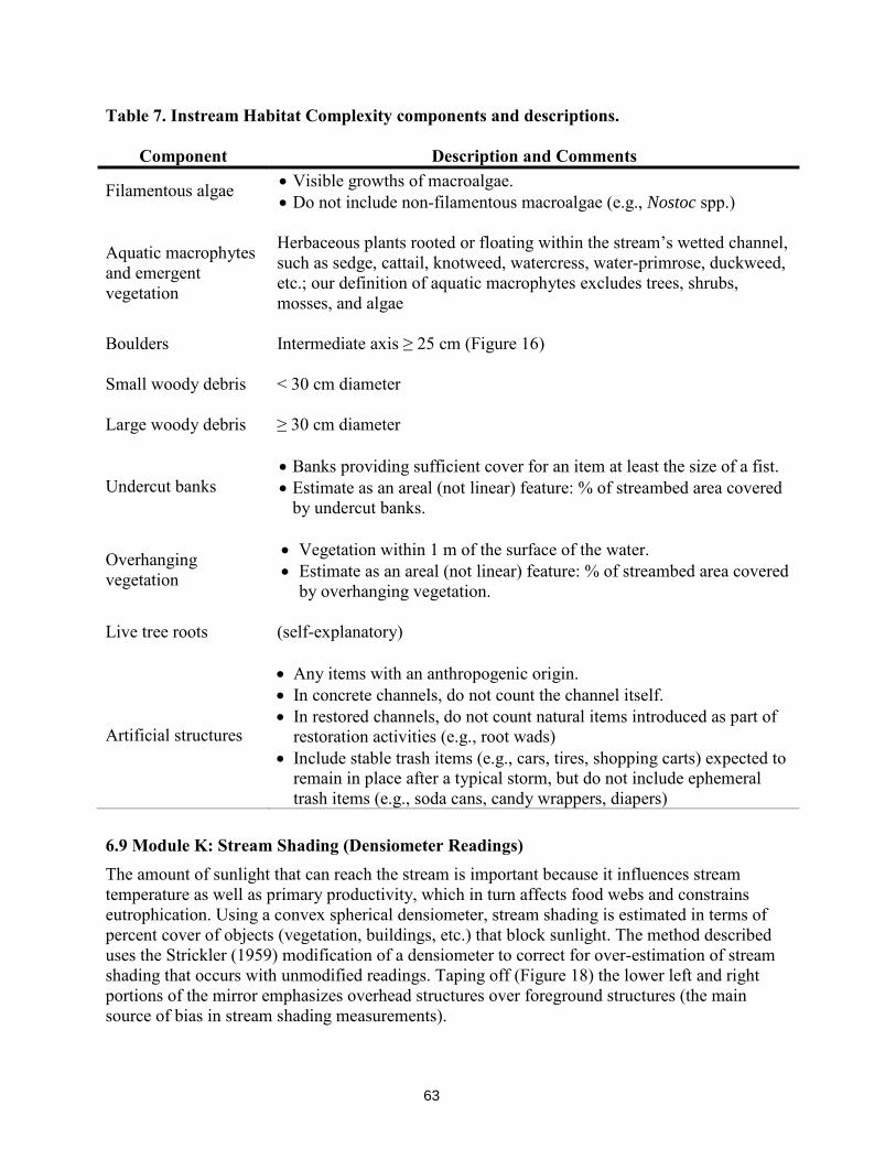
63
Table 7. Instream Habitat Complexity components and descriptions.
Component Description and Comments
Filamentous algae • Visible growths of macroalgae. • Do not include non-filamentous macroalgae (e.g., Nostoc spp.)
Aquatic macrophytes and emergent vegetation
Herbaceous plants rooted or floating within the stream’s wetted channel, such as sedge, cattail, knotweed, watercress, water-primrose, duckweed, etc.; our definition of aquatic macrophytes excludes trees, shrubs, mosses, and algae
Boulders Intermediate axis ≥ 25 cm (Figure 16) Small woody debris < 30 cm diameter Large woody debris ≥ 30 cm diameter
Undercut banks • Banks providing sufficient cover for an item at least the size of a fist. • Estimate as an areal (not linear) feature: % of streambed area covered
by undercut banks.
Overhanging vegetation
• Vegetation within 1 m of the surface of the water. • Estimate as an areal (not linear) feature: % of streambed area covered
by overhanging vegetation. Live tree roots (self-explanatory)
Artificial structures
• Any items with an anthropogenic origin. • In concrete channels, do not count the channel itself. • In restored channels, do not count natural items introduced as part of
restoration activities (e.g., root wads) • Include stable trash items (e.g., cars, tires, shopping carts) expected to
remain in place after a typical storm, but do not include ephemeral trash items (e.g., soda cans, candy wrappers, diapers)
6.9 Module K: Stream Shading (Densiometer Readings) The amount of sunlight that can reach the stream is important because it influences stream temperature as well as primary productivity, which in turn affects food webs and constrains eutrophication. Using a convex spherical densiometer, stream shading is estimated in terms of percent cover of objects (vegetation, buildings, etc.) that block sunlight. The method described uses the Strickler (1959) modification of a densiometer to correct for over-estimation of stream shading that occurs with unmodified readings. Taping off (Figure 18) the lower left and right portions of the mirror emphasizes overhead structures over foreground structures (the main source of bias in stream shading measurements).
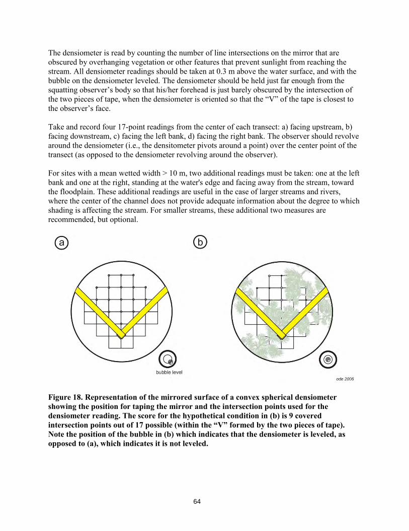
64
The densiometer is read by counting the number of line intersections on the mirror that are obscured by overhanging vegetation or other features that prevent sunlight from reaching the stream. All densiometer readings should be taken at 0.3 m above the water surface, and with the bubble on the densiometer leveled. The densiometer should be held just far enough from the squatting observer’s body so that his/her forehead is just barely obscured by the intersection of the two pieces of tape, when the densiometer is oriented so that the “V” of the tape is closest to the observer’s face. Take and record four 17-point readings from the center of each transect: a) facing upstream, b) facing downstream, c) facing the left bank, d) facing the right bank. The observer should revolve around the densiometer (i.e., the densitometer pivots around a point) over the center point of the transect (as opposed to the densiometer revolving around the observer). For sites with a mean wetted width > 10 m, two additional readings must be taken: one at the left bank and one at the right, standing at the water's edge and facing away from the stream, toward the floodplain. These additional readings are useful in the case of larger streams and rivers, where the center of the channel does not provide adequate information about the degree to which shading is affecting the stream. For smaller streams, these additional two measures are recommended, but optional.
Figure 18. Representation of the mirrored surface of a convex spherical densiometer showing the position for taping the mirror and the intersection points used for the densiometer reading. The score for the hypothetical condition in (b) is 9 covered intersection points out of 17 possible (within the “V” formed by the two pieces of tape). Note the position of the bubble in (b) which indicates that the densiometer is leveled, as opposed to (a), which indicates it is not leveled.
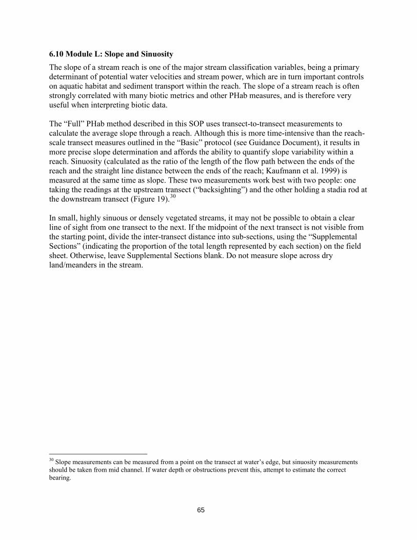
65
6.10 Module L: Slope and Sinuosity The slope of a stream reach is one of the major stream classification variables, being a primary determinant of potential water velocities and stream power, which are in turn important controls on aquatic habitat and sediment transport within the reach. The slope of a stream reach is often strongly correlated with many biotic metrics and other PHab measures, and is therefore very useful when interpreting biotic data. The “Full” PHab method described in this SOP uses transect-to-transect measurements to calculate the average slope through a reach. Although this is more time-intensive than the reach-scale transect measures outlined in the “Basic” protocol (see Guidance Document), it results in more precise slope determination and affords the ability to quantify slope variability within a reach. Sinuosity (calculated as the ratio of the length of the flow path between the ends of the reach and the straight line distance between the ends of the reach; Kaufmann et al. 1999) is measured at the same time as slope. These two measurements work best with two people: one taking the readings at the upstream transect (“backsighting”) and the other holding a stadia rod at the downstream transect (Figure 19).30 In small, highly sinuous or densely vegetated streams, it may not be possible to obtain a clear line of sight from one transect to the next. If the midpoint of the next transect is not visible from the starting point, divide the inter-transect distance into sub-sections, using the “Supplemental Sections” (indicating the proportion of the total length represented by each section) on the field sheet. Otherwise, leave Supplemental Sections blank. Do not measure slope across dry land/meanders in the stream.
30 Slope measurements can be measured from a point on the transect at water’s edge, but sinuosity measurements should be taken from mid channel. If water depth or obstructions prevent this, attempt to estimate the correct bearing.
66
Figure 19. Use of an autolevel to measure slope of sampling reach. Although slope and sinuosity are measured independently, always record the two data points at each location. An autolevel should always be used for reaches with a slope of ≤ 1. Either a clinometer or an autolevel may be used for reaches with a slope of > 1%, and sometimes (e.g., in steep areas that are also heavily vegetated) a clinometer is preferable for logistical reasons. If a reach is visually estimated to be close to 1%, use the autolevel. An autolevel or hand level measures the elevation difference (rise) between transects; the distance between transects (run) is also required for a slope calculation. Conversely, if a clinometer is used, the percent slope is recorded directly. Do not measure slope across dry land (e.g., across a meander bend). 6.10.1 Slope - autolevel method Step 1. Identify a good spot to set up the autolevel (ideally near the middle of the reach, if there is good visibility from this location to both Transects A and K). The autolevel should be positioned on stable, and preferably flat, ground. Set the height of the autolevel to comfortable eye level for the operator. Level the plane of view of the autolevel by centering its bubble. Start by adjusting placement and length of the tripod legs, and then fine-tune the adjustment using the knobs on the autolevel.
67
Step 2. Begin “shooting” the change in elevation of the water level of the stream from transect to transect. Try to start with one of the outer transects (like K)31. Have a crew member at Transect K hold the stadia rod at water’s edge and perpendicular to the ground. Viewing through the autolevel (and focusing as necessary), look at the stadia rod and record, to the smallest demarcation on the stadia rod, the height at which the autolevel line of view (i.e., the middle line in the viewfinder) hits. Record this information on the “Slope and Bearing Form” on the field sheet32, and then have the stadia rod holder proceed to the next transect (e.g., Transect J), again holding the base of the stadia rod at water’s edge. Very carefully, rotate the head of the autolevel so that it points to the new stadia rod location. If executed correctly, the bubble should still be centered while in this new orientation, without any further height adjustments to the autolevel or tripod. If the autolevel is displaced from its original position, it will no longer be possible to take a height measurement of Transect J’s water surface, relative to that of Transect K, to determine the slope between the two transects. In this case, the elevation must be measured anew (see Step 3). Step 3. If there is a point along the reach at which there is no longer a clear line of sight from the autolevel to the stadia rod positioned at the transect, at water’s edge (or if the length of the stadia rod is exceeded in a steep reach, or if the autolevel is bumped out of position before all the measurements are done), a new location must be set up for the autolevel. In order to maintain a relationship with water heights of the various transects already measured, it will be necessary to “re-shoot” the height of the water at the last transect for which a valid measurement was attained. From there, assuming there is no more disturbance to the position of the autolevel, the remaining transects can be sighted from the new position. On the Slope and Bearing Form corresponding to autolevel use, indicate the transect at which the autolevel’s position has been changed (i.e., list the transect that was measured from the original and the new positions twice on the datasheet: once for the original position, and once for the new). Also indicate the segment lengths or distance between main transects (i.e., 15 m, 25 m or other). These data will later be used to determine the slopes between transects and for the reach as a whole. 6.10.2 Slope - clinometer method Step 1. Stand erect next to the stadia rod (held perpendicularly to the ground) on level ground and a tie a highly visible piece of flagging around the rod at eye level. Then, beginning with the upper transect (Transect K), stand where the wetted margin intersects with the transect, and have a second person hold the flagged stadia rod perpendicularly to the ground at the wetted margin of the next downstream transect (Transect J). Step 2. Use the clinometer to measure the percent slope of the water surface between the upstream transect and the downstream transect by sighting to the flagged position on the stadia 31 It does not matter if the measurements of slope and/or elevation difference are determined starting at the upstream or downstream end of the reach, but they must be reported as positive numbers. 32 Only the elevation difference (cm) will be recorded in the database. “Raw” stadia rod readings can be written on the hard copy sheets for reference and calculations but they will not be stored in the database.

68
rod, and record the value in the "Slope and Bearing Form” section of the field sheets. The clinometer gives both percent slope and degree of the slope (the measurements differ by a factor of ~2.2), so be careful to read and record percent slope rather than degrees slope. Percent slope is read from the scale on the right hand side when looking through most clinometers (but confirm this with the owner’s manual for your own model). Step 3. Continue measuring slope at each one of the transects. Note that when moving from transect to transect, the clinometer reader must stand exactly where the stadia rod had been placed during the previous reading. Step 4. If the stream reach geometry makes it difficult to sight a line between transects, divide the distance into two or three sections and record the slope and the proportion of the total segment length between transects for each of these sections in the appropriate boxes on the slope form (“Supplemental Segment”). 6.10.3 Sinuosity Step 1. Take a compass reading from the center of each main transect to the center of the next main transect downstream and record this bearing to the nearest degree in the "Slope and Bearing Form” section of the field sheet. Bearing measurements should always be taken from the upstream to downstream transect. Step 2. Proceed downstream to the next transect pair (I-J) and continue to record slope and bearing between each pair of transects until measurements have been recorded for all transects. 6.11 Module M: Photographs Take a minimum of four (4) photographs of the reach at the following locations: a) Transect A, facing upstream, b) Transect F, facing upstream, c) Transect F, facing downstream, and d) Transect K, facing downstream. It is also desirable, albeit optional, to take a photograph at Transect A, facing downstream and Transect K, facing upstream to document conditions immediately adjacent to the reach. Use digital photographs. Record the image numbers on the front page of the field form under “Photographs”. An easy way to keep track of which site each series of photographs belongs to is to take a close-up of the front data sheet (containing legible station code and date) for that site prior to taking the series of photos.
69
7. PHYSICAL HABITAT INTER-TRANSECT-BASED MEASUREMENTS
Although most measures are taken near the main transects, a few measures are also recorded at the “inter-transects” located at the midpoint between main transects. These measures are: 1) Wetted Width, 2) Substrate Measurements (“Pebble Count”)/Depth/CPOM/Cobble Embeddedness/Algal and Macrophyte Cover, and 3) Flow Habitats. 7.1 Module C (part two): Inter-transect Wetted Width Measure wetted width the same way it was measured for the main transects. 7.2 Modules D, E, and F (part two): Substrate Measurements, Depth, CPOM, and Algal/Macrophyte Percent Cover Collect particle size measurements, water depth, CPOM, embeddedness and algal and macrophyte cover data the same way they were collected for the main transects. 7.3 Module N: Flow Habitats Because many BMIs and algae prefer specific flow and substrate microhabitats, the proportional representation of these habitats in a reach is often of interest in bioassessments. Like the riparian and instream PHab measures, this procedure produces a semi-quantitative measure consisting of 10 transect-based visual estimates. A description of flow habitat types used for this SOP is provided in Table 7. These flow habitat types are products of geology, slope, and discharge, and one habitat type may change into another as water levels increase or decrease; therefore, the habitat types should be recorded at the time of sampling. On the inter-transect field sheet, record to the nearest 5% percentages of the various flow habitats present within the region between the upstream inter-transect and downstream inter-transect bracketing each main transect (the total percentage of flow habitats for each stream section must total 100%). Although these definitions differ from geomorphological definitions presented in other hydrologic references, they were developed to produce more easily standardized and objective categories that improve data comparability. Please adhere to the definitions used in this text when employing this SOP.
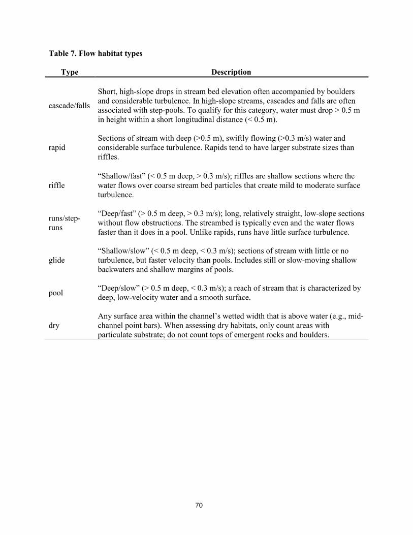
70
Table 7. Flow habitat types
Type Description
cascade/falls
Short, high-slope drops in stream bed elevation often accompanied by boulders and considerable turbulence. In high-slope streams, cascades and falls are often associated with step-pools. To qualify for this category, water must drop > 0.5 m in height within a short longitudinal distance (< 0.5 m).
rapid Sections of stream with deep (>0.5 m), swiftly flowing (>0.3 m/s) water and considerable surface turbulence. Rapids tend to have larger substrate sizes than riffles.
riffle “Shallow/fast” (< 0.5 m deep, > 0.3 m/s); riffles are shallow sections where the water flows over coarse stream bed particles that create mild to moderate surface turbulence.
runs/step-runs
“Deep/fast” (> 0.5 m deep, > 0.3 m/s); long, relatively straight, low-slope sections without flow obstructions. The streambed is typically even and the water flows faster than it does in a pool. Unlike rapids, runs have little surface turbulence.
glide “Shallow/slow” (< 0.5 m deep, < 0.3 m/s); sections of stream with little or no turbulence, but faster velocity than pools. Includes still or slow-moving shallow backwaters and shallow margins of pools.
pool “Deep/slow” (> 0.5 m deep, < 0.3 m/s); a reach of stream that is characterized by deep, low-velocity water and a smooth surface.
dry Any surface area within the channel’s wetted width that is above water (e.g., mid-channel point bars). When assessing dry habitats, only count areas with particulate substrate; do not count tops of emergent rocks and boulders.
71
8. PHYSICAL HABITAT REACH-BASED MEASUREMENTS
8.1 Module O: Stream Discharge Stream discharge is the volume of water that moves past a point in a given amount of time and is generally reported as cubic feet per second. Discharge affects the concentration of nutrients, fine sediments, and pollutants, and its measurement is critical for understanding impacts of disturbances such as impoundments, water withdrawals, and water augmentation. Discharge is also closely related to many habitat characteristics including temperature regimes, physical habitat diversity, and habitat connectivity. As a direct result of these relationships, stream discharge is often also a strong predictor of biotic community composition. Since stream volume can vary significantly on many temporal scales (diurnal, seasonal, inter-annual), it can also be very useful for understanding variation in stream condition. For this SOP, a single discharge measurement is conducted in order to estimate discharge through the sampling reach. There is no prescribed point in the reach where the measurement should be taken; rather, it is up to the discretion of the field crew, depending upon streambed morphology and flow. It is preferable to take the discharge measurement in a section where flow velocities are > 0.15 m/s and most depths are > 15 cm, but slower velocities and shallower depths can be used, if necessary. If flow volume is sufficient for a transect-based “velocity-area” discharge calculation (Section 8.1.1), this is the preferred method. If the velocity meter probe cannot be submerged, but there is visible flow, the following two options are available: 1) use of the Neutrally Buoyant Object approach (which is the second most preferred method to measure flow) OR 2) a visual estimation of the velocity based on best professional judgment. In small, shallow streams with complex substrate, it may still be difficult to accurately measure discharge, even where water movement is obvious. If visual estimation is used, the velocity measurement must be denoted with a “visual estimate” flag in the data base. Data for this parameter are entered in the “Discharge Measurements” section of the field sheet. 8.1.1 Velocity Area Method The layout for discharge measurements under the velocity-area method is illustrated in Figure 20. Flow velocity should be measured with either a Swoffer Instruments propeller-type flow meter or a Marsh-McBirney inductive probe flow meter with a top-setting rod. Refer to the manufacturer instrument manual for calibration procedures. Step 1. Select the best location (cross-section) in the reach to place a transect across which to measure discharge. This does not need to coincide with any of the main or inter-transects where other PHab measurements were taken, however it should lie within, or very near, the stream reach being assessed. Choose a cross section with flow that is as uniform as possible (i.e., hydraulically smooth), and with the simplest possible cross-sectional geometry. It is helpful to move bed material or other obstacles to create a more uniform cross-section before beginning the discharge measurements, but this cannot be done after measurements have begun, or it will skew results.
72
Step 2. Measure the wetted width of the discharge transect and divide this into 10 to 20 equal segments. The use of more segments gives a better discharge calculation, but is impractical in small channels. At least 10 intervals should be used when stream width permits, but interval width should not be < 15 cm. Step 3. Record the distance from the bank to the end of the first interval. Using the top-setting rod, measure and record the median depth of the first interval (Figure 20). Step 4. Stand downstream of the transect and off to the side of the probe in order to avoid interfering with the flow measurement. Set the probe of the flow meter at the midpoint of the first interval along the discharge transect, facing upstream perpendicularly to the direction of flow. If necessary, a thin piece of flagging tape can be attached to the top-setting rod and submerged to identify the direction of flow and thus inform proper angling of the probe. Determine the depth of the water and adjust the top-setting rod accordingly, such that the probe is held at a depth of 0.6 of the total stream depth. This position generally approximates average velocity in the water column. See Figure 20 for positioning detail. Refer to the top-setting rod owner’s manual for further instructions on positioning of probe height. Step 5. Allow the flow velocity meter to equilibrate for at least 15 seconds, and then record velocity to the nearest ft/s. If the option is available, use the flow-averaging setting on the flow meter33. Record the flow velocity. Under very low flow conditions, flow velocity meters may register readings of zero even when there is noticeable flow. In these situations, record the appropriate ResQualCode (ND, Not Detected) and QACode (FLV, Velocity too low to be measured) and leave the Result field blank in the database. The Instrument Detection Limit (IDL) should be noted for the instrument used. In areas that are too shallow to measure velocity, use the Neutrally Buoyant Object method. If the flow is moving upstream (such as near banks or in an eddy), point the probe into the flow and record the velocity with a negative symbol on the field sheet. Record an "NG" QA flag with this result in the database in order to identify the result as a negative value. Step 6. Complete Steps 3 through 5 on the remaining intervals. Frequently, the first and last intervals have depths and velocities of zero.
33 Set the averaging interval to at least 15 seconds (30 seconds if velocity is > 2 ft/s) and record the 15secondaverage velocity measurement for each segment.
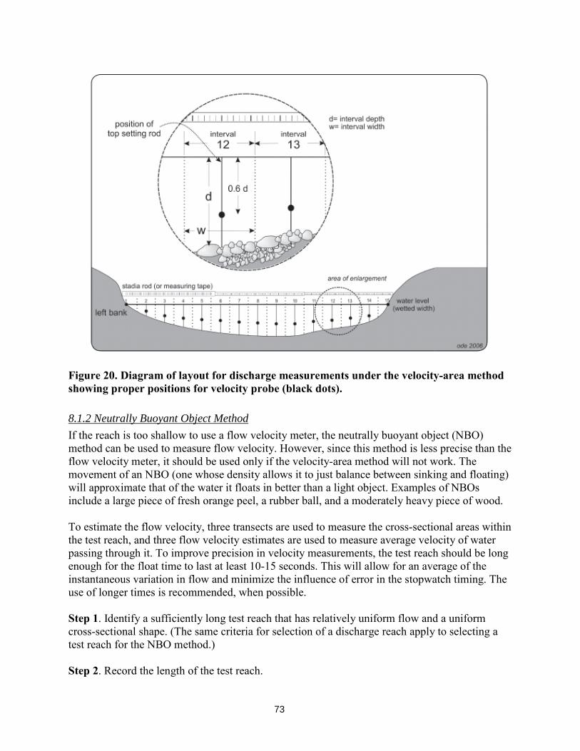
73
Figure 20. Diagram of layout for discharge measurements under the velocity-area method showing proper positions for velocity probe (black dots). 8.1.2 Neutrally Buoyant Object Method If the reach is too shallow to use a flow velocity meter, the neutrally buoyant object (NBO) method can be used to measure flow velocity. However, since this method is less precise than the flow velocity meter, it should be used only if the velocity-area method will not work. The movement of an NBO (one whose density allows it to just balance between sinking and floating) will approximate that of the water it floats in better than a light object. Examples of NBOs include a large piece of fresh orange peel, a rubber ball, and a moderately heavy piece of wood. To estimate the flow velocity, three transects are used to measure the cross-sectional areas within the test reach, and three flow velocity estimates are used to measure average velocity of water passing through it. To improve precision in velocity measurements, the test reach should be long enough for the float time to last at least 10-15 seconds. This will allow for an average of the instantaneous variation in flow and minimize the influence of error in the stopwatch timing. The use of longer times is recommended, when possible. Step 1. Identify a sufficiently long test reach that has relatively uniform flow and a uniform cross-sectional shape. (The same criteria for selection of a discharge reach apply to selecting a test reach for the NBO method.) Step 2. Record the length of the test reach.
74
Step 3. Measure the cross sectional area of the test reach in three places (an “Upper Section”, a “Middle Section” and a “Lower Section”). Three evenly-spaced cross sections are preferred, but a single one may be used if the cross section through the test reach is uniform (e.g., in a concrete channel). On the “Float Reach Cross Section” of the field sheet, record the width once, and the depth at five equally-spaced positions, across each of the three cross sections of the test reach. Step 4. Place the NBO in the water upstream of the test reach and record the length of time (in seconds) that it takes for the object to pass between the reach’s upstream and downstream boundaries. Repeat this twice more for a total of three timed “floats”. 8.2 Module P: Post-Sampling Observations: Qualitative Reach Measures EPA’s Rapid Bioassessment Procedures (RBPs, Barbour et al. 1999) include a set of 10 visual criteria for assessing instream and riparian habitat. The RBP has been used in the CSBP since its first edition (1995), and thus this information is often valuable for comparison to legacy datasets. The criteria also have a useful didactic role, since they help force the user to quantify key features of the physical environment where bioassessment samples are collected. The full suite of RBP stream habitat visual estimates are not covered in this SOP because they are generally replaced by more quantitative measurements of similar variables. However, three of the RBP measures (“Epifaunal Substrate/Cover”, “Sediment Deposition”, and “Channel Alteration”) have been found to be reasonably repeatable and thus are included. Record observations in the “Additional Habitat Characterization” section of the field sheet.
75
8. OPTIONAL SUPPLEMENTAL MEASURES
Optional measures to supplement this SOP may be included in stream assessments according to program needs. These include the excess sediment index (sometimes referred to as log relative bed stability, LRBS) and additional measurements collected for the LRBS calculations (Kaufmann et al. 1999), such as tallies of woody debris and thalweg. The NRSA Field Operations Manual (USEPA 2009) provides more details on collecting these data types. Large woody debris (logs, snags, branches, etc.) that is capable of obstructing flow when the channel is at bankfull (i.e., just short of flood) stage contributes to the “roughness” of a channel. The effect of this variable is to reduce water velocity and thereby reduce the stream’s competence to move substrate particles. The NRSA (Section 6.2.4.2) protocol tallies all woody debris with a diameter > 10 cm (~4”) into one of 12 size classes based on the length and width of each object. Tallies are conducted in the zone between the main transects. A stream’s thalweg is a longitudinal profile that connects the deepest points of successive cross-sections of the stream. The thalweg defines the primary path of water flow through the reach. Thalweg measurements (NRSA; Section 5.2.7) perform many functions in the NRSA protocols, producing measurements for the excess sediment calculations (residual pool volume, stream size, channel complexity) and flow habitat variability.
76
9. REFERENCES
Barbour, M.T., J. Gerritsen, B.D. Snyder and J.B. Stribling. 1999. Revision to rapid
bioassessment protocols for use in stream and rivers: periphyton, BMIs and fish. EPA 841-D-97-002. U.S. Environmental Protection Agency. Washington DC.
Davies A.L. and J.H.R. Gee. 1993. A simple algae sampler for algal biomass estimates in
streams. Freshwater Biology 30: 47-51. Fetscher, A.E. and K. McLaughlin. 2008. Incorporating Bioassessment Using Freshwater Algae
into California’s Surface Water Ambient Monitoring Program (SWAMP). Prepared for the California State Water Resources Control Board.
Fetscher A.E., L.B. Busse and P.R. Ode 2009. Standard Operating Procedures for Collecting
Stream Algae Samples and Associated Physical Habitat and Chemical Data for Ambient Bioassessments in California. California State Water Resources Control Board Surface Water Ambient Monitoring Program (SWAMP) Bioassessment SOP 002. (updated May 2010)
Fetscher, A.E., R. Stancheva, J.P. Kociolek, R.G. Sheath, E.D. Stein, R.D. Mazor, P.R Ode, and
L.B. Busse. 2014. Development and comparison of stream indices of biotic integrity using diatoms vs. non-diatom algae vs. a combination. Journal of Applied Phycology 26:433-450.
Harrington, J.M. 1995. California stream bioassessment procedures. California Department of
Fish and Game, Water Pollution Control Laboratory. Rancho Cordova, CA. Harrington, J.M. 1999. California stream bioassessment procedures. California Department of
Fish and Game, Water Pollution Control Laboratory. Rancho Cordova, CA. Harrington, J.M. 2002. California stream bioassessment procedures. California Department of
Fish and Game, Water Pollution Control Laboratory. Rancho Cordova, CA. Kaufmann, P.R., P.L. Levine, E.G. Robison, C. Seeliger, and D.V. Peck. 1999. Quantifying
Physical Habitat in Wadeable Streams. EPA 620/R-99/003. U.S. Environmental Protection Agency.
Kelly, M.G., A. Cazaubon, E. Coring, A. Dell’Uomo, L. Ector, B. Goldsmith, H. Guasch, J.
Hürlimann, A. Jarlman, B. Kawecka, J. Kwandrans, R. Laugaste, E.-A. Lindstrøm12, M. Leitao, P. Marvan, J. Padis´ak, E. Pipp, J. Prygie, E. Rott, S. Sabater, H. van Dam, and J. Vizinet. 1998. Recommendations for the routine sampling of diatoms for water quality assessments in Europe. Journal of Applied Phycology 10: 215–224.
Mount, J.F. 1995. California rivers and streams: the conflict between fluvial process and land
use. Univ of California Press.

77
Ode P. 2007. SWAMP Bioassessment Procedures: Standard operating procedures for collecting benthic macroinvertebrate samples and associated physical and chemical data for ambient bioassessment in California. Available from http://www.swrcb.ca.gov/water_issues/programs/swamp/docs/swamp_sop_bio.pdf
Peck, D. V., A. T. Herlihy, B. H. Hill, R. M. Hughes, P. R. Kaufmann, D. Klemm, J. M.
Lazorchak, F. H. McCormick, S. A. Peterson, P. L. Ringold, T. Magee, and M. Cappaert. 2006. Environmental Monitoring and Assessment Program-Surface Waters Western Pilot Study: Field Operations Manual for Wadeable Streams. U.S. Environmental Protection Agency, Washington, D.C. EPA/620/R-06/003.
Round, F.E. 1991. Diatoms in river water-monitoring studies. Journal of Applied Phycology
3:129-145. Southern California Coast Water Research Project. 2009. Southern California Regional
Watershed Monitoring Program Bioassessment Quality Assurance Project Plan. Stevenson, R.J. and L.L. Bahls. 1999. Periphyton protocols. Chapter 6 in: M.T. Barbour, J.
Gerritsen, B.D. Snyder, and J.B. Stribling (eds.), Rapid Bioassessment Protocols for use in Streams and Wadeable Rivers. Second Edition. EPA/841-B-99-002. US Environmental Protection Agency, Office of Water. Washington, DC.
Stevenson, R.J. and S.L. Rollins. 2006. Ecological assessments with benthic algae. In: Hauer,
F.R. And G.A. Lamberti, eds. Methods in Stream Ecology. Pp. 785-803. Strickler, G. S., 1959. Use of the densiometer to estimate density of forest canopy on permanent
sample plots. USDA Forest Service, Pacific Northwest Forest and Range Exp. Sta. Research Note 180, Portland, Oregon, 5 pp.
Sylte, T. and Fischenich, C. 2002. Techniques for measuring substrate embeddedness (No.
ERDC-TN-EMRRP-SR-36). Engineer Research and Development Center, Vicksburg MS Environmental Lab.
SWAMP. 2008. Quality Assurance Program Plan of the California Surface Water Ambient
Monitoring Program. http://www.waterboards.ca.gov/water_issues/programs/swamp/docs/qapp/qaprp082209.pdf
Tetra Tech 2006. Technical Approach to Develop Nutrient Numeric Endpoints for California.
Tetra Tech, Inc. http://rd.tetratech.com/e pa/Documents/CA_NNE_July_Final.pdf USEPA. 2009. National Rivers and Streams Assessment: Field Operations Manual. EPA-841-B-
07-009. U.S. Environmental Protection Agency, Washington, DC. Wolman, M.G. 1954. A method of sampling coarse river-bed material: Transactions of the
American Geophysical Union 35: 951-956.

78
Woodard, M.E., J. Slusark, and P.R. Ode. 2012. Standard Operating Procedures for Laboratory Processing and Identification of Benthic Macroinvertebrates in California. California State Water Resources Control Board Surface Water Ambient Monitoring Program (SWAMP) Bioassessment SOP 003. http://www.swrcb.ca.gov/water_issues/programs/swamp/docs/bmi_lab_sop_final.pdf
79
10. GLOSSARY
Aliquot – a measured portion of a sample, or subsample Allochthonous – derived from a source external to the stream channel (e.g., riparian vegetation
as a source of organic matter) as opposed to autochthonous, which indicates a source inside the stream channel (e.g., algae or macrophytes rooted in the stream)
Ambient bioassessment – monitoring that is intended to describe general biotic condition as opposed to a diagnosis of sources of impairment
Ash-free dry mass (AFDM) – the portion, by mass, of a dried sample that is represented by organic matter; the concentration of AFDM per stream surface area sampled is often used as a surrogate for algal biomass
Bankfull – the bankfull channel is the zone of maximum water inundation in a normal flow year (one- to two-year flood events)
Benthic algae – algae that are attached to, or have at one point been anchored to, the stream bottom, in contrast to planktonic algae which are free-floating in the water column
Benthic macroinvertebrates (BMI) – bottom-dwelling invertebrates large enough to be seen with the unaided eye
Biofilm – a matrix/film adhering to stream substrates and consisting of microorganisms (e.g., algae, fungi, bacteria, protozoans) and detritus
Chlorophyll a – primary light receptor/photosynthetic pigment in algae and cyanobacteria and higher plants; the concentration of this pigment per stream surface area sampled provides an estimate of algal biomass
Coarse particulate organic matter (CPOM) –particles of decaying organic material, such as leaves and twigs, that are between 1 and 10 mm in diameter and suitable for consumption by BMIs in the “shredder” functional feeding group
Cobble embeddedness – The percent of surface area of cobble-sized particles (64-250 mm) buried by fine particles (<2.0 mm diameter)
Composite sample - volume of all the liquid material amassed during sampling, including water used for rinsing substrate and sampling devices.
Cyanobacteria – historically referred to as “blue-green” algae, but actually chlorophyll-a containing prokaryotes that are capable of photosynthesis and co-occur with “true” (i.e., eukaryotic) benthic algae in streams; useful as a bioindicator, and field-sampled and laboratory-processed as soft-bodied algae
Depositional – habitats in the stream that are dominated by slow-moving water, such as pools, where deposition of materials from the water column is more likely to occur than erosion (or (re)suspension) of loose bed materials
Diatom – a unicellular golden-brown alga (Bacillariophyta) that possesses a rigid, silicified (silica-based) cell wall in the form of a “pill box”
Elutriation – the process of using a liquid (water) to separate denser material (e.g., stream sediments) from lighter materials (organic particles and benthic organisms). -.
Erosional – habitats in the stream that are dominated by fast-moving water, such as riffles, where stream power is more likely to facilitate erosion (suspension) of loose benthic material than deposition
Fines – substrate particles < 0.06 mm diameter (not gritty to the touch)
80
Guidance Document – a companion document to this SOP that provides more information on the various applications of the indicators described herein, as well as recommendations for where and when to use this SOP. It also provides more detailed information on how to deal with special circumstances that may be encountered during bioassessment sampling.
Homogenate – mixture of algae liquid composite sample and finely chopped fragments of macroalgae that comprises the quantitative sample for the diatom taxonomic ID, chlorophyll a, and AFDM subsamples
Index of Biotic Integrity (IBI) – a quantitative assessment tool that uses information about the composition of one or more assemblages of organisms to make inferences about condition, or ecological health, of the environments they occupy (e.g., algae or benthic macroinvertebrates)
Inter-transects – transects established at points equidistant between the main transects Macroalgae – soft bodied algae that form macroscopically discernible filaments, mats, or
globose structures Macrophyte, aquatic – herbaceous, vascular plant rooted or floating within the stream’s wetted
channel, such as sedge, cattail, knotweed, watercress, water-primrose, duckweed, etc.; our definition of aquatic macrophytes excludes trees, shrubs, mosses, and algae
Microalgae – diatoms and microscopic soft-bodied algae (can co-occur with other microorganisms in a biofilm)
Prospecting mine – a hand-excavated, hard-rock mining hole that is open to the surface (common in the Sierra Nevada)
Reach – a linear segment of the stream channel Reachwide benthos (RWB) – method for biotic assemblage sample collection that does not
target a specific substrate type, but rather objectively selects sampling locations across the reach, allowing for any of a number of substrate types to be represented in the resulting composite sample
Riparian – an area of land and vegetation adjacent to a stream that has a direct effect on the stream by providing shade, habitat for wildlife, contributing allochthonous organic matter, modulating water levels via evaporative transpiration, etc.
Sinuosity – the ratio of the length of the flow path between the ends of the reach and the straight line distance between the ends of the reach (Kaufmann et al. 1999)
Soft-bodied algae – non-diatom algal taxa; for the purposes of this SOP, cyanobacteria are included in this assemblage
Substrate – the composition of a streambed, including both inorganic and organic particles Target coordinates – the nominal or tentative location of a sampling site, which may differ from
the actual location from which samples are collected Thalweg – the thalweg defines the primary path of water flow through the reach; it is often
inferred by depth for practical purposes, but is not always the deepest point Transects – lines drawn perpendicular to the path of flow used for standardizing biotic sampling
and data collection locations Wadeable stream – a stream that can be sampled by field crews wearing chest waders
(generally < 1 meter deep for at least half the reach) Wetted width – the width of the channel containing water (the active channel), defined as the distance between the sides of the channel at the point where substrates are no longer surrounded by surface water