Embed Size (px)
Citation preview
Thèse de Doctorat de l’Université de Mons
Spécialité :Sciences Mathématiques
Symmetries of solutions for nonlinearSchrödinger equations:
Numerical and Theoretical approaches
présenté par
Grumiau Christopher
pour l’obtention du grade de Docteur en Sciences.
Thèse soutenue le 24 Septembre 2010 devant le jury composé de :
Pr. Denis Bonheure, Université Libre de BruxellesPr. Catherine Finet, Université de MonsPr. Karl-Goswin Grosse-Erdmann, Université de Mons (Secrétaire)Pr. Joseph McKenna, University of Connecticut (Président)Pr. Serge Nicaise, Université de Valenciennes et du Hainaut CambrésisPr. Christophe Troestler, Université de Mons (Directeur)Pr. Michel Willem, Université Catholique de Louvain
Année académique 2010–2011

2
Acknowledgments –Remerciements
To start, I would like to thank all the members of my jury who will spendtime to read and judge this work. I am especially grateful to my supervisor,Professor Christophe Troestler, who accepted me in his team as PhD-studentand assistant, despite the fact that I did not follow his courses during my master!It probably was “risky” (for both of us) but, at the end, I am very proud tobecome (I hope...) his first “mathematical son”. Thanks a lot for the support,discussions and help during these last years. I also express my thankfulness toProfessor Joe McKenna who welcomed me at UCONN during four months. Itwas really a great pleasure and experience for me to spend several months in anAmerican university.
Then, I am grateful to all my collaborators for the work realised togetherand the good “team spirit” during the different workshops. More specifically,I thank all my co-authors: Denis Bonheure, Vincent Bouchez, Enea Parini,Christophe Troestler and Jean Van Schaftingen. Without the dynamism andexperience of these mathematicians, some parts of this work would never havebeen done. A special thanks goes to Vincent Bouchez for the very long days ofwork (and more) in Louvain-la-Neuve or in Mons. By “more”, of course, I referto the several times where, at the end of a very tiring day (okay, it is a little bitexaggerated!), we played tennis, badminton or squash. I hope to continue this“sport friendship” in the future... I am thinking I owe you one game, right (Iam joking)? In the same spirit, I also remember different games with JonathanDi Cosmo and joggings in the streets of Cologne with Sébastien De Valeriola.
3
4
I also would like to thank all the current and past young mathematicianswith whom I not only shared the same office but also jokes and good ambience(during lunches, parties, world cup of soccer, tennis games,...). I thank Bertrandand Fabien who read some parts of this PhD. I also have a thought for anymember of the mathematic department with whom I have discussed or worked.I remember different “giggles” with Stéphanie Bridoux during the preparationof courses or exams. I also thank members of the secretary for the help inadministration stuff and the help to find classrooms (not always so easy!!!).
I also would like to thank the “Communauté française de Belgique”, the“Fonds national de la recherche scientifique” and the “European Science Foun-dation” for the financial support given for different stays abroad.
Last but not least, I would like to say a few words in French to thank myfamily.
Tout d’abord, je suis reconnaissant envers maman pour le soutien financierdurant la licence et, beaucoup plus important, émotionnel durant la thèse. Je laremercie de m’avoir soutenu dans les études qui me plaisaient et pour la liberté,en tout domaine, qu’elle m’a laissée. Ensuite, je remercie ma copine, Laetitia,pour son amour et le fait d’être auprès de moi. Je la remercie également d’avoirrévisé son alphabet (je plaisante...) afin de m’aider dans la remise en ordre desfeuilles d’examen ainsi que de son anglais afin de m’écouter parfois répéter mesexposés. Dans le même esprit, je remercie ma soeur Stéphanie ayant de tempsen temps effectué la même tâche ! ! !
Je sais que pour eux le travail de thésard assistant leur semble, commentdire, un mélange d’étrange, de non bien-défini, d’enviable et de fou (ce ne sontpeut-être pas les bons mots mais je ne vois pas mieux). D’un côté, entre lespériodes de recherche “intensive” et les cours à donner, nous sommes en mêmetemps chercheur et enseignant. D’un autre côté, nous gardons notre liberté etla participation à des conférences nous fait voir du pays. D’ailleurs, pour eux,une certaine ambiguïté perdure concernant ce dernier point : j’ai beau leur direque le travail est “acharné” en conférence, le doute semble toujours de misedans leurs esprits (sur ce que l’on fait en dehors de nos frontières). Bien-sûr,quand on regarde les photos, on ne peut pas non plus totalement leur donnertort... Néanmoins, j’espère que l’exposé de ce travail permettra de dissiper unpeu leurs doutes à ce sujet.
5
Finalement, je remercie Papa, Fabrice et Marcel pour les trajets à l’aéroportet le soutien ainsi que Lucas (qui me demande régulièrement si le boulot sepasse bien), ma belle-soeur Caroline, mes beaux-parents ainsi que tous ceuxque j’aurais malencontreusement oubliés.

6
Contents
Summary in French – Résumé en français 9
Introduction 13
1 Lane–Emden problem with DBC 311.1 Asymptotic behavior . . . . . . . . . . . . . . . . . . . . . . . 35
1.1.1 Upper bound . . . . . . . . . . . . . . . . . . . . . . . 361.1.2 Lower bound . . . . . . . . . . . . . . . . . . . . . . . 391.1.3 Conclusion: limit equation and variational characteri-
zation . . . . . . . . . . . . . . . . . . . . . . . . . . . 411.2 Nondegenerate case: dimE2 = 1 . . . . . . . . . . . . . . . . . 43
1.2.1 Method based on the implicit function theorem . . . . . 431.2.2 Example: the rectangle . . . . . . . . . . . . . . . . . . 45
1.3 Radial domains . . . . . . . . . . . . . . . . . . . . . . . . . . 461.3.1 Study of E2 . . . . . . . . . . . . . . . . . . . . . . . . 471.3.2 Method based on the “Radial IFT” . . . . . . . . . . . . 501.3.3 Examples: the ball and the annulus . . . . . . . . . . . 51
1.4 General domains . . . . . . . . . . . . . . . . . . . . . . . . . 521.4.1 A uniqueness result . . . . . . . . . . . . . . . . . . . . 521.4.2 An abstract symmetry theorem . . . . . . . . . . . . . . 551.4.3 Example: the square . . . . . . . . . . . . . . . . . . . 56
1.5 Symmetry breaking . . . . . . . . . . . . . . . . . . . . . . . . 591.5.1 Perturbation of the Laplacian operator . . . . . . . . . . 601.5.2 Symmetry breaking on rectangles . . . . . . . . . . . . 62
7
8 Contents
1.6 What about ground state solutions? . . . . . . . . . . . . . . . . 65
2 Nodal line structure of least energy nodal solutions 692.1 Convergence in C 1(Ω) . . . . . . . . . . . . . . . . . . . . . . 702.2 Nodal line structure . . . . . . . . . . . . . . . . . . . . . . . . 72
2.2.1 Asymptotic results . . . . . . . . . . . . . . . . . . . . 722.2.2 The convex case . . . . . . . . . . . . . . . . . . . . . 732.2.3 The non-simply connected case . . . . . . . . . . . . . 73
3 Schrödinger and q-Laplacian problem 773.1 Positive definite Schrödinger problem . . . . . . . . . . . . . . 80
3.1.1 Asymptotic behavior . . . . . . . . . . . . . . . . . . . 803.1.2 Symmetries extending . . . . . . . . . . . . . . . . . . 813.1.3 Symmetry breaking of least energy nodal solutions on
rectangles . . . . . . . . . . . . . . . . . . . . . . . . . 823.1.4 Example: non-zero constant potential . . . . . . . . . . 82
3.2 q-Laplacian Lane–Emden problem . . . . . . . . . . . . . . . . 843.2.1 Existence of solutions . . . . . . . . . . . . . . . . . . 843.2.2 Asymptotic results . . . . . . . . . . . . . . . . . . . . 88
4 General nonlinearities 934.1 Asymptotic behavior . . . . . . . . . . . . . . . . . . . . . . . 98
4.1.1 Limit equation . . . . . . . . . . . . . . . . . . . . . . 994.1.2 Upper bound . . . . . . . . . . . . . . . . . . . . . . . 994.1.3 Lower bound . . . . . . . . . . . . . . . . . . . . . . . 103
4.2 Symmetries . . . . . . . . . . . . . . . . . . . . . . . . . . . . 1064.2.1 Uniqueness around an eigenfunction . . . . . . . . . . . 1064.2.2 Symmetry breaking of least energy nodal solutions on
rectangles . . . . . . . . . . . . . . . . . . . . . . . . . 1074.3 Examples: explicit nonlinearities . . . . . . . . . . . . . . . . . 109
4.3.1 Superlinear perturbation of Lane–Emden Problem . . . 1094.3.2 Exponential growth . . . . . . . . . . . . . . . . . . . . 1114.3.3 Sum of powers . . . . . . . . . . . . . . . . . . . . . . 113
4.4 Super-lower homogeneity assumption . . . . . . . . . . . . . . 115
Contents 9
5 Lane–Emden problem with NBC 1175.1 Asymptotic symmetries when p→ 2 . . . . . . . . . . . . . . . 121
5.1.1 Asymptotic behavior . . . . . . . . . . . . . . . . . . . 1215.1.2 Symmetries . . . . . . . . . . . . . . . . . . . . . . . . 1225.1.3 Symmetry breaking of least energy nodal solutions on
rectangles . . . . . . . . . . . . . . . . . . . . . . . . . 1245.1.4 Examples . . . . . . . . . . . . . . . . . . . . . . . . . 125
5.2 Ground state solutions for p large . . . . . . . . . . . . . . . . 1305.2.1 The ground state solutions are not radial for p large . . . 1315.2.2 Bifurcation results . . . . . . . . . . . . . . . . . . . . 1315.2.3 Specific case: a ball . . . . . . . . . . . . . . . . . . . . 1335.2.4 Numerical symmetry breaking and conjecture . . . . . . 137
6 General potentials: mountain pass algorithms 1396.1 Constrained steepest descent method for
indefinite problems . . . . . . . . . . . . . . . . . . . . . . . . 1446.1.1 Convergence up to a subsequence . . . . . . . . . . . . 1476.1.2 Convergence . . . . . . . . . . . . . . . . . . . . . . . 150
6.2 Application and conjecture . . . . . . . . . . . . . . . . . . . . 1516.2.1 Convergence of the generalized MPA for Schrödinger
problems . . . . . . . . . . . . . . . . . . . . . . . . . 1526.2.2 Illustration and conjecture . . . . . . . . . . . . . . . . 153
A Some classical results 155
Notations 157
Bibliography 160

10 Contents
Summary in French –Résumé en français
Cette thèse est consacrée à l’étude de l’équation de Schrödinger non-linéaire
−∆u(x)+V (x)u(x) = f (u(x)), x dans Ω, (1)
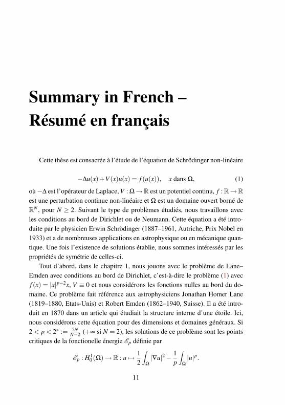
où−∆ est l’opérateur de Laplace, V : Ω→R est un potentiel continu, f : R→Rest une perturbation continue non-linéaire et Ω est un domaine ouvert borné deRN , pour N ≥ 2. Suivant le type de problèmes étudiés, nous travaillons avecles conditions au bord de Dirichlet ou de Neumann. Cette équation a été intro-duite par le physicien Erwin Schrödinger (1887–1961, Autriche, Prix Nobel en1933) et a de nombreuses applications en astrophysique ou en mécanique quan-tique. Une fois l’existence de solutions établie, nous sommes intéressés par lespropriétés de symétrie de celles-ci.
Tout d’abord, dans le chapitre 1, nous jouons avec le problème de Lane–Emden avec conditions au bord de Dirichlet, c’est-à-dire le problème (1) avecf (x) = |x|p−2x, V ≡ 0 et nous considérons les fonctions nulles au bord du do-maine. Ce problème fait référence aux astrophysiciens Jonathan Homer Lane(1819–1880, Etats-Unis) et Robert Emden (1862–1940, Suisse). Il a été intro-duit en 1870 dans un article qui étudiait la structure interne d’une étoile. Ici,nous considérons cette équation pour des dimensions et domaines généraux. Si2 < p < 2∗ := 2N
N−2 (+∞ si N = 2), les solutions de ce problème sont les pointscritiques de la fonctionelle énergie Ep définie par
Ep : H10 (Ω)→ R : u 7→ 1
2
∫Ω
|∇u|2− 1p
∫Ω
|u|p.
11
12 Summary in French
En 1973 (resp. 1997), A. Ambrosetti et P. H. Rabinowitz (resp. A. Castro,J. Cossio et J. M. Neuberger) ont prouvé que ce problème possède, en plus dela solution nulle, au moins une solution de signe constant (resp. nodale) d’éner-gie minimale. En 1979, B. Gidas, W. N. Ni et L. Nirenberg ont montré queles solutions qui ne changent pas de signe, sur un domaine convexe, possèdentles symétries du domaine. Dans le chapitre 1, nous nous demandons si, pourdes domaines généraux, les solutions nodales d’énergie minimale respectentégalement l’entièreté ou une partie des symétries du domaine (parité et impa-rité par rapport aux hyperplans de symétrie). Ces résultats sont liés aux articles[14, 39] écrits en collaboration avec D. Bonheure, V. Bouchez, C. Troestler etJ. Van Schaftingen. En résumé, nous montrons que les solutions nodales d’éner-gie minimale :
– sur un domaine rectangulaire, pour p proche de 2, sont paires par rapportà la grande médiane et impaires par rapport à la petite ;
– sur un domaine radial, pour p proche de 2, sont paires par rapport à N−1directions orthogonales et impaires par rapport à la dernière ;
– sur un domaine carré, pour p proche de 2, sont impaires par rapport aucentre. De plus, nous conjecturons qu’elles sont impaires par rapport àune diagonale.
Pour de grandes valeurs de p, nous obtenons l’existence de rectangles pourlesquels les solutions nodales d’énergie minimale ne respectent pas les symé-tries du domaine. Nous obtenons donc une brisure de symétrie : il n’est paspossible de généraliser nos résultats de symétrie pour de grandes valeurs de p.Remarquons que notre technique retrouve les résultats de B. Gidas, W. N. Ni etL. Nirenberg pour l’étude des solutions de signe constant d’énergie minimale,au moins pour p petit. Elle donne également une méthode alternative lorsque ledomaine est non-convexe.
Dans le chapitre 2, concernant les solutions nodales, nous « généralisons »le problème à des domaines non-symétriques. En fait, nous étudions la struc-ture de la ligne nodale des solutions nodales d’énergie minimale. Il s’agit d’untravail [38] en collaboration avec C. Troestler. Nous montrons que pour des do-maines convexes de dimension 2, pour p proche de 2, la ligne nodale intersectetoujours le bord du domaine. De plus, nous construisons un domaine connexenon-convexe (en fait, il est même non-simplement connexe) sur lequel, pour p
Summary in French 13
proche de 2, la ligne nodale n’intersecte pas le bord du domaine.Les chapitres 3 à 5 sont consacrés à des problèmes plus généraux que celui
de Lane–Emden. Dans le chapitre 3, dans un premier temps, nous montrons quesous l’hypothèse que −∆ +V soit défini positif, les mêmes résultats de symé-trie que ceux obtenus dans le chapitre 1 sont valables. Ensuite, nous étudionsl’équation de Schrödinger pour le cas du q-Laplacien
−∆qu = |u|p−2u, dans Ω,
u = 0, sur ∂Ω,(2)
où ∆qu := div(|∇u|q−2∇u), pour 1 < q < p. Ce travail [36] est une collaborationavec E. Parini. Nous obtenons que les solutions qui ne changent pas de signe(resp. nodales) d’énergie minimale convergent à un changement d’échelle prèsvers des solutions non-nulles du problème aux valeurs propres
−∆qu = λ |u|q−2u, dans Ω,
u = 0, sur ∂Ω,(3)
quand p→ q. Malheureusement, le manque de linéarité du q-Laplacien nousempêche d’obtenir des résultats de symétrie.
Dans le chapitre 4, nous travaillons avec des non-linéarités plus générales.En particulier, nous sommes intéressés à des non-linéarités non-homogènes.Nous donnons des hypothèses sur f de manière à ce que les résultats de symétriedonnés dans le premier chapitre restent valables. Par exemple, pour certainesvaleurs de λ , les non-linéarités suivantes respecteront toutes nos hypothèses :
λ t|t|p−2 +(p−2)t|t|q−2, λ t(et2 −1)p−2 ou λ t
(k
∑i=1
αi|t|βi(p−2)
).
Ce travail [12] est une collaboration avec D. Bonheure et V. Bouchez.Dans le chapitre 5, il sera temps de travailler avec les conditions au bord de
Neumann. Nous travaillons avec le problème (1) particularisé à V ≡ 1, f (x) =|x|p−2x, p > 2 et nous considérons les fonctions à dérivée nulle sur le bord dudomaine. Ce chapitre est inspiré des travaux [12, 13] écrits en collaborationavec D. Bonheure et V. Bouchez. Si 2 < p < 2∗ := 2N
N−2 (+∞ si N = 2), lessolutions de ce problème sont les points critiques de la fonctionelle énergie Ep
14 Summary in French
définie par
Ep : H1(Ω)→ R : u 7→ 12
∫Ω
|∇u|2 +u2− 1p
∫Ω
|u|p.
Nous montrons tout d’abord que les techniques développées dans le chapitre 1sont toujours valables. Ceci nous permet d’étudier les symétries des solutionsde signe constant et nodales d’énergie minimale lorsque p est proche de 2. Enparticulier, concernant les solutions de signe constant d’énergie minimale, nousobtenons directement qu’elles respectent toutes les symétries du domaine. Deplus, nous améliorons ce résultat et obtenons que ces solutions doivent êtreégales à la constante 1 ou −1. Au contraire des conditions au bord de Dirichletoù les solutions de signe constant d’énergie minimale respectent les symétriesdu domaine pour tout p, on sait que ceci n’est plus nécessairement le cas pourNeumann, au moins pour de grandes dimensions. Ici, en toute dimension, nousmontrons l’existence de cette brisure de symétrie : les solutions 1 et −1 nepeuvent plus être des solutions d’énergie minimale pour p > 1 + λ2, où λ2 estla seconde valeur propre de −∆ + id avec les conditions au bord de Neumanndans H1(Ω). Nous conjecturons d’ailleurs que 1+λ2 est optimal.
Pour finir, rappelons que dans le chapitre 3 nous avons étudié le cas de po-tentiels V non-nuls tels que−∆+V est défini positif. Si cette dernière hypothèsen’est pas vérifiée, le problème se complique. Ceci est lié au fait que la solution0 n’est plus un minimum local de la fonctionelle énergie. Néanmoins, il estpossible de montrer l’existence d’une solution non-nulle au problème. Dans cedernier chapitre, nous développons un procédé numérique de type « mountainpass » permettant d’approcher cette solution. Nous prouvons la convergencede l’algorithme. L’implémentation nous permet de construire une conjecturesur les symétries des solutions de signe constant d’énergie minimale lorsque lepotentiel V est constant et −∆ +V possède des valeurs propres négatives. Cetravail [37] est une collaboration avec C. Troestler.
Tout au long de cette thèse, nous utiliserons l’implémentation que nousavons faite des algorithmes du “mountain pass” et du “mountain pass modifié”afin d’illustrer nos résultats.
Introduction
During my schooling, I remember some professors teaching me that thereexists an “universal method” to solve a scientific problem:
1. to observe (e.g. by making experiences);
2. to model (e.g. by using equations);
3. “to solve the modelization” (e.g. by approaching, finding or “studying”solutions of the equations).
In physics, many and many problems, and especially these studied during highschool (just think about the use of the Newton equation, about simple mechanicproblems,...), were solved following this method. In fact, many times, differen-tial equations were used as a model (sometimes without saying it explicitely).Certainly, as we all know, it is not always so simple. Depending on the currentproblem, every point may be very difficult to solve: sometimes it can take lotsof time or cost lots of money to make the observations and experiences, some-times we need to simplify the problem (by making assumptions on our envi-ronment,...) to obtain a satisfying model, sometimes the solutions of the modelcan only be approached and not exactly obtained, and sometimes the model isjust impossible to solve (or we have no idea to obtain or approach solutions).In this PhD-thesis, we deal with the third point of the “universal method” forsome differential equations more or less related to physical problems. To bemore precise, the differential equations studied here are mainly related to thewell-known nonlinear Schrödinger equation
−∆u(x)+V (x)u(x) = f (u(x)), x in Ω, (4)
15
16 Introduction
where ∆ denotes the Laplacian operator, V : Ω→ R is a continuous potential,f : R→ R is a nonlinear differentiable perturbation and Ω is an open boundedconnected domain in RN , for N ≥ 2. Depending on the problem, we workwith Dirichlet boundary conditions (DBC; i.e. u = 0 on the boundary ∂Ω) orNeumann boundary conditions (NBC; i.e. ∂ν u = 0 on ∂Ω where ∂ν denotesthe normal derivative). This equation is named after the theoretical physicistErwin Schrödinger (1887–1961, Austria, Nobel Prize in 1933) and has lots ofapplications in astrophysics, quantum mechanics,...
Once the existence of solutions established, we are interested in properties(like symmetry properties related to the symmetries of the domain) of thesesolutions.
To start, we work with the so-called Lane–Emden problem (LEP) withDirichlet boundary conditions. It is the nonlinear elliptic boundary value prob-lem (4) with V ≡ 0, f (x) = |x|p−2x for 2 < p, N = 3 and Ω a ball. It is namedafter the astrophysicists Jonathan Homer Lane (1819–1880, USA) and RobertEmden (1862–1940, Switzerland). This Problem (LEP) was introduced for thefirst time in 1870 by J. Lane [47]. He published the first paper studying theinternal structure of a star. Physically, solutions of the Lane–Emden problemgive the variation of pressure and density, for the gravitational potential of aself-gravitating, of a spherical polytropic fluid. Here, we study this equation forgeneral dimensions (N ≥ 2) and general domains (Ω is open bounded). If p issubcritical, i.e. p < 2∗ := 2N
N−2 (2∗ = +∞ if N = 2), the problem is variational.It means that the solutions of Problem (LEP) are the critical points of a C 1-functional E , i.e. functions u such that dE (u) = 0. In our case, the functional,named energy functional, is defined on the Sobolev space1 H1
0 (Ω) by
Ep(u) :=12
∫Ω
|∇u|2− 1p
∫Ω
|u|p.
A priori, we just obtain weak solutions. Nevertheless, by the regularity theory(see e.g. [19]), we get classical solutions2. If necessary, readers can find a ref-erence in the Master’s thesis [35]: in it, existence of solutions, some symmetryresults and numerical examples have already been studied in details. This work
1H10 (Ω) is the closure in L2(Ω) of the space C 2
0 (Ω) for the classical norm(∫
Ω|∇u|2
)1/2.2Functions in C 2(Ω)∩C (Ω)
Introduction 17
u0
Ep
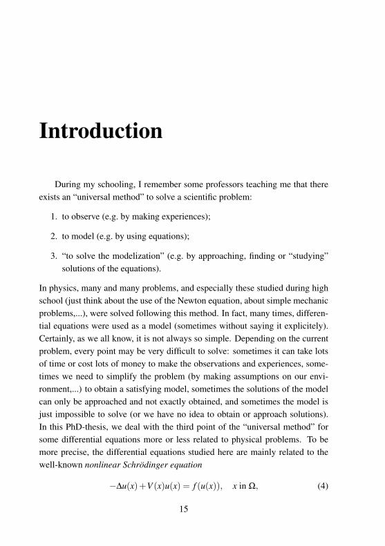
Figure 1: Energy Functional.
was the starting point of this PhD-thesis. Readers can freely download it frommy web page3.
Clearly, the zero constant function is a solution of the Lane–Emden Prob-lem (LEP) with DBC. Let us remark that the energy Ep respects a Mountain-Pass type structure (see Figure 1). We mean that
• 0 is a strict local minimum of Ep;
• for any u 6= 0, there exists one and only one critical point of Ep restrictedto tut>0;
• for any u 6= 0, limt→+∞ Ep(tu) =−∞.
Concerning other solutions, in 1973, A. Ambrosetti and P. H. Rabinowitzproved that Problem (LEP) has a ground state solution, i.e. a non-trivial solutionwith minimal energy [6]. Moreover, this typical solution must be a one-signedfunction. To obtain this, they minimized Ep on
v ∈ H10 (Ω)\0 :
⟨dEp(v),v
⟩= 0
.
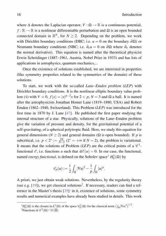
Concerning symmetries, in 1979, B. Gidas, W. N. Ni and L. Nirenberg [32]showed, using the elegant and now celebrated “moving planes” technique, that,on a convex domain, they inherit all the symmetries of the domain (e.g. even-ness w.r.t. hyperplanes, see Figure 2). Moreover, on balls, a positive (resp. neg-ative) ground state solution respects a Schwarz symmetry, i.e. u can be writtenas u(x) = u(|x|) and u(r) is nonincreasing (resp. nondecreasing). So, the sym-metries of ground state solutions are already well-known at least for convexdomains.
18 Introduction
0.0
0.5
1.0
1.5
2.0
2.5
Z−1.0
−0.6
−0.2
0.2
0.6
1.0
X
−1.0
−0.6
−0.2
0.2
0.6
1.0
Y
Figure 2: Ground state solution of the Lane–Emden problem on a ball.
0.0
0.5
1.0
1.5
2.0
2.5
3.0
3.5
Z
−3
−2
−1
0
1
2
3
X
−1
0
1Y
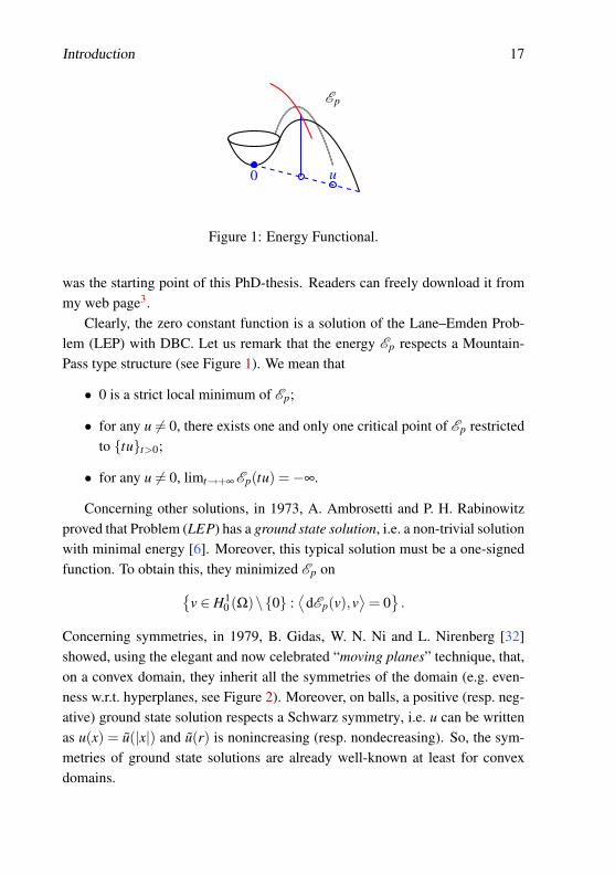
Figure 3: Ground state solution on an annulus and a dumblebell.
For a non-convex domain, the “moving planes” method does not work. Inour case, on an annulus, H. Brezis and L. Nirenberg (see e.g. [20]) proved thata symmetry breaking can occur for large p (see Figure 3). We also can observeon Figure 3 a symmetry breaking on the dumblebell, a connected domain.
Turning to nodal solutions, A. Castro, J. Cossio and J. M. Neuberger [23]proved in 1997 the existence of a solution with minimal energy among all sign-changing ones, which is therefore referred to as the least energy nodal solution(l.e.n.s.) of Problem (LEP). Readers can also find reference in [68]. Sinceground state solutions inherit the symmetries of the domain, at least if Ω is
3http://staff.umh.ac.be/Grumiau.Christopher/
Introduction 19
ξ
AB
CD
AD DB C
u
u(A)> u(B) = u(C)> u(D)
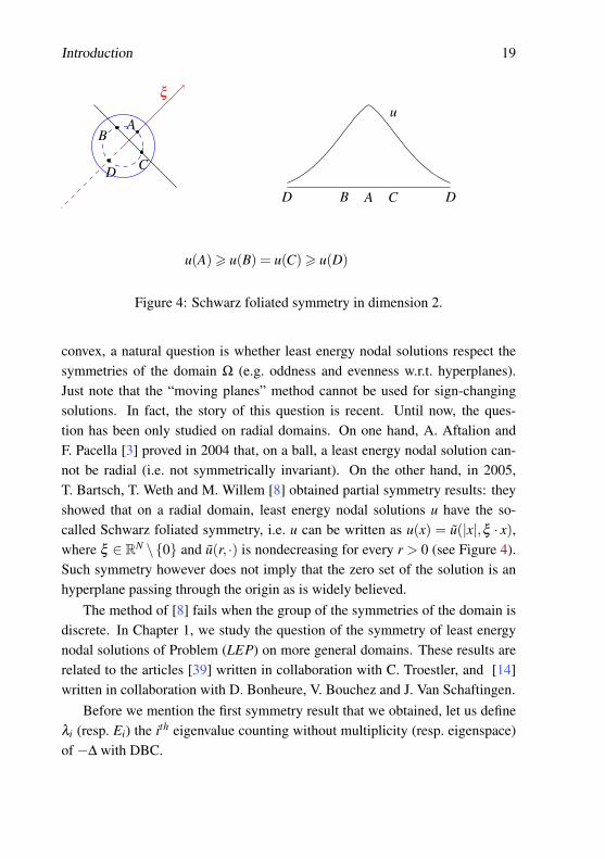
Figure 4: Schwarz foliated symmetry in dimension 2.
convex, a natural question is whether least energy nodal solutions respect thesymmetries of the domain Ω (e.g. oddness and evenness w.r.t. hyperplanes).Just note that the “moving planes” method cannot be used for sign-changingsolutions. In fact, the story of this question is recent. Until now, the ques-tion has been only studied on radial domains. On one hand, A. Aftalion andF. Pacella [3] proved in 2004 that, on a ball, a least energy nodal solution can-not be radial (i.e. not symmetrically invariant). On the other hand, in 2005,T. Bartsch, T. Weth and M. Willem [8] obtained partial symmetry results: theyshowed that on a radial domain, least energy nodal solutions u have the so-called Schwarz foliated symmetry, i.e. u can be written as u(x) = u(|x|,ξ · x),where ξ ∈ RN \0 and u(r, ·) is nondecreasing for every r > 0 (see Figure 4).Such symmetry however does not imply that the zero set of the solution is anhyperplane passing through the origin as is widely believed.
The method of [8] fails when the group of the symmetries of the domain isdiscrete. In Chapter 1, we study the question of the symmetry of least energynodal solutions of Problem (LEP) on more general domains. These results arerelated to the articles [39] written in collaboration with C. Troestler, and [14]written in collaboration with D. Bonheure, V. Bouchez and J. Van Schaftingen.
Before we mention the first symmetry result that we obtained, let us defineλi (resp. Ei) the ith eigenvalue counting without multiplicity (resp. eigenspace)of −∆ with DBC.
20 Introduction
Theorem 1. Assume that λ2 is simple, i.e. dimE2 = 1. Then, for p close to2 and any reflection R such that R(Ω) = Ω, least energy nodal solutions ofProblem (LEP) have, with respect to R, the same symmetries or antisymmetriesthan second eigenfunctions of −∆ with DBC. Moreover, for p close to 2, theleast energy nodal solution is unique up to symmetries of the domain and amultiplicative factor of value −1.
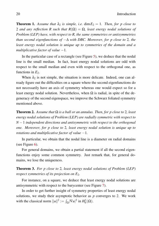
In the particular case of a rectangle (see Figure 5), we deduce that the nodalline is the small median. In fact, least energy nodal solutions are odd withrespect to the small median and even with respect to the orthogonal one, asfunctions in E2.
When λ2 is not simple, the situation is more delicate. Indeed, one can al-ready figure out the difficulties on a square where the second eigenfunctions donot necessarily have an axis of symmetry whereas one would expect so for aleast energy nodal solution. Nevertheless, when Ω is radial, in spite of the de-generacy of the second eigenspace, we improve the Schwarz foliated symmetrymentioned above.
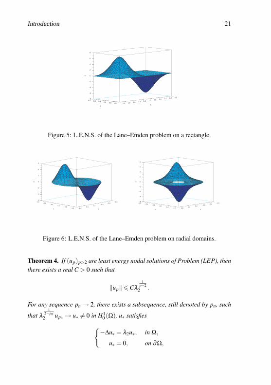
Theorem 2. Assume that Ω is a ball or an annulus. Then, for p close to 2, leastenergy nodal solutions of Problem (LEP) are radially symmetric with respect toN−1 independent directions and antisymmetric with respect to the orthogonalone. Moreover, for p close to 2, least energy nodal solution is unique up torotations and multiplicative factor of value −1.
In particular, we obtain that the nodal line is a diameter on radial domains(see Figure 6).
For general domains, we obtain a partial statement if all the second eigen-functions enjoy some common symmetry. Just remark that, for general do-mains, we lose the uniqueness.
Theorem 3. For p close to 2, least energy nodal solutions of Problem (LEP)respect symmetries of its projection on E2.
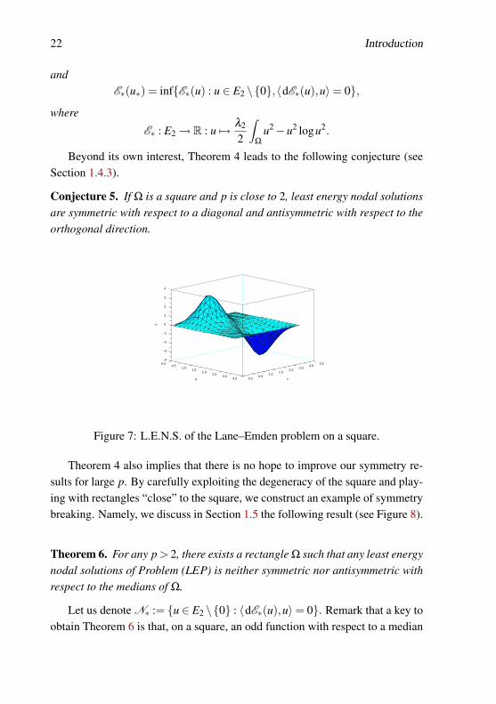
For instance, on a square, we deduce that least energy nodal solutions areantisymmetric with respect to the barycenter (see Figure 7).
In order to get further insight of symmetry properties of least energy nodalsolutions, we study their asymptotic behavior as p converges to 2. We workwith the classical norm ‖u‖2 :=
∫Ω|∇u|2 in H1
0 (Ω).
Introduction 21
−8
−6
−4
−2
0
2
4
6
8
Z
0.00.20.40.60.81.01.21.41.61.82.0X
0.0 0.2 0.4 0.6 0.8 1.0Y
Figure 5: L.E.N.S. of the Lane–Emden problem on a rectangle.
−6
−4
−2
0
2
4
6
Z
−1.0−0.6
−0.20.2
0.61.0 X
−1.0−0.6
−0.20.2
0.61.0Y
−8
−6
−4
−2
0
2
4
6
8
Z
−1.0−0.6
−0.20.2
0.61.0
X
−1.0−0.6
−0.20.2
0.61.0
Y
Figure 6: L.E.N.S. of the Lane–Emden problem on radial domains.
Theorem 4. If (up)p>2 are least energy nodal solutions of Problem (LEP), thenthere exists a real C > 0 such that
‖up‖6Cλ
1p−2
2 .
For any sequence pn→ 2, there exists a subsequence, still denoted by pn, such
that λ
12−pn
2 upn → u∗ 6= 0 in H10 (Ω), u∗ satisfies−∆u∗ = λ2u∗, in Ω,
u∗ = 0, on ∂Ω,
22 Introduction
andE∗(u∗) = infE∗(u) : u ∈ E2 \0,〈dE∗(u),u〉= 0,
where
E∗ : E2→ R : u 7→ λ2
2
∫Ω
u2−u2 logu2.
Beyond its own interest, Theorem 4 leads to the following conjecture (seeSection 1.4.3).
Conjecture 5. If Ω is a square and p is close to 2, least energy nodal solutionsare symmetric with respect to a diagonal and antisymmetric with respect to theorthogonal direction.
−4
−3
−2
−1
0
1
2
3
4
Z
0.00.5
1.01.5
2.02.5
3.03.5
Y
0.00.5
1.01.5
2.02.5
3.03.5X
Figure 7: L.E.N.S. of the Lane–Emden problem on a square.
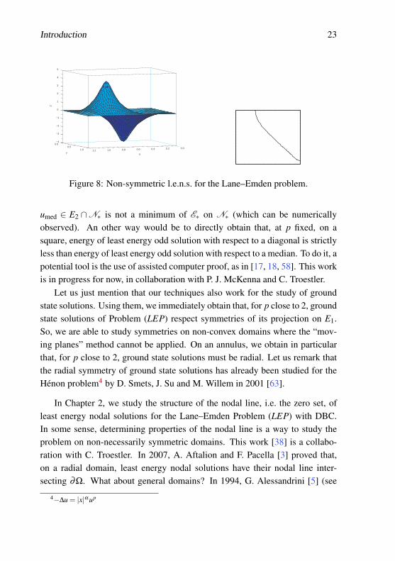
Theorem 4 also implies that there is no hope to improve our symmetry re-sults for large p. By carefully exploiting the degeneracy of the square and play-ing with rectangles “close” to the square, we construct an example of symmetrybreaking. Namely, we discuss in Section 1.5 the following result (see Figure 8).
Theorem 6. For any p > 2, there exists a rectangle Ω such that any least energynodal solutions of Problem (LEP) is neither symmetric nor antisymmetric withrespect to the medians of Ω.
Let us denote N∗ := u ∈ E2 \0 : 〈dE∗(u),u〉= 0. Remark that a key toobtain Theorem 6 is that, on a square, an odd function with respect to a median
Introduction 23
−4
−3
−2
−1
0
1
2
3
4
5
Z
0.00.20.40.60.81.01.2
X
0.00.5
1.0Y
Figure 8: Non-symmetric l.e.n.s. for the Lane–Emden problem.
umed ∈ E2 ∩N∗ is not a minimum of E∗ on N∗ (which can be numericallyobserved). An other way would be to directly obtain that, at p fixed, on asquare, energy of least energy odd solution with respect to a diagonal is strictlyless than energy of least energy odd solution with respect to a median. To do it, apotential tool is the use of assisted computer proof, as in [17, 18, 58]. This workis in progress for now, in collaboration with P. J. McKenna and C. Troestler.
Let us just mention that our techniques also work for the study of groundstate solutions. Using them, we immediately obtain that, for p close to 2, groundstate solutions of Problem (LEP) respect symmetries of its projection on E1.So, we are able to study symmetries on non-convex domains where the “mov-ing planes” method cannot be applied. On an annulus, we obtain in particularthat, for p close to 2, ground state solutions must be radial. Let us remark thatthe radial symmetry of ground state solutions has already been studied for theHénon problem4 by D. Smets, J. Su and M. Willem in 2001 [63].
In Chapter 2, we study the structure of the nodal line, i.e. the zero set, ofleast energy nodal solutions for the Lane–Emden Problem (LEP) with DBC.In some sense, determining properties of the nodal line is a way to study theproblem on non-necessarily symmetric domains. This work [38] is a collabo-ration with C. Troestler. In 2007, A. Aftalion and F. Pacella [3] proved that,on a radial domain, least energy nodal solutions have their nodal line inter-secting ∂Ω. What about general domains? In 1994, G. Alessandrini [5] (see
4−∆u = |x|α up
24 Introduction
also [51]) proved that the nodal line of the non-zero second eigenfunctions of−∆ intersects ∂Ω at exactly two points when Ω⊆ R2 is convex. By combiningAlessandrini’s result with Chapter 1, we establish the following result.
Proposition 7. For a convex domain Ω ⊆ R2, not necessarily possessing anysymmetry, the zero set of least energy nodal solutions intersects ∂Ω, at least forp close to 2.
Then, M. Hoffmann-Ostenhof, T. Hoffmann-Ostenhof and N. Nadirashvi-li [40], in 1997, proved that there exists a connected but non-simply connecteddomain Ω such that dimE2 = 1 and the nodal line of the second eigenfunctionsdoes not intersect ∂Ω. This result implies the following one.
Proposition 8. If the convexity assumption is removed, the zero set may wellnot touch ∂Ω anymore.
It is a conjecture that, on a simply connected domain, the nodal line alwaysintersects ∂Ω. However, at this time, this is not proved to be true even for thelinear case.
In chapter 3 to 5, we are dealing with various problems. We would like toknow if asymptotic and symmetry results obtained in Chapter 1 are also workingfor V 6≡ 0, other nonlinearities or NBC. In Chapter 3, we study perturbations ofthe linear part of Problem (LEP).
First, we work with a non-zero potential V :−∆u(x)+V (x)u(x) = |u(x)|p−2u(x), x in Ω,
u(x) = 0, x on ∂Ω.(5)
We give assumptions on V such that the results explained in Chapter 1 remainvalid. We establish the following result.
Proposition 9. If the operator −∆+V is positive definite5, we have
1. for p close to 2, a ground state solution verifies the symmetries of itsprojection on E1, the first eigenspace of −∆+V ;
2. for p close to 2, a least energy nodal solution verifies the symmetries ofits projection on E2, the second eigenspace of −∆+V .
5All eigenvalues of the operator are positive.
Introduction 25
Up to some symmetry assumptions on the eigenfunctions of −∆ +V , wealso obtain the existence of a symmetry breaking on some rectangles.
Second, we study the asymptotic behavior of ground state solutions andleast energy nodal solutions for the q-Laplacian Lane–Emden problem withDBC:
−∆qu = |u|p−2u, in Ω,
u = 0, on ∂Ω,(6)
where ∆qu := div(|∇u|q−2∇u), 1 < q < p < q∗ (with q∗ = nqn−q if q < n, and
q∗ = +∞ otherwise). This work [36] is a collaboration with E. Parini. Thesolutions are the critical points of the energy functional Ep,q defined on theSobolev space6 W 1,q
0 (Ω) and given by
Ep,q(u) :=1q
∫Ω
|∇u|q− 1p
∫Ω
|u|p.
For q = 2, Problem (6) corresponds to the classical Lane–Emden problemwith DBC already studied. For q 6= 2, things seem to become more complicated,due in particular to the lack of linearity of the q-Laplacian.
Because of this, so far, we have not been able to conclude symmetries ofground state solutions and least energy nodal solutions. In fact, even for thelimit problem
−∆qu = λ |u|q−2u, in Ω,
u = 0, on ∂Ω,(7)
the problem has not yet completely been solved (see Chapter 3 for details).About asymptotic behavior, it is reasonable to suppose that ground state solu-tions and least energy nodal solutions of Problem (6) converge when p con-verges to q, after being suitably scaled, to non-zero solutions of Problem (7).This result will be proved in Chapter 3.
In Chapter 4, we point out that results given in Chapter 1 also work withmore general nonlinearities fp. In particular, the technique developed in Chap-ter 1 does not depend on the homogeneity of the nonlinear term. In this chapter,we recall assumptions on the nonlinearity fp such that the energy functional
6W 1,q0 (Ω) is the closure in Lq(Ω) of the space C 2
0 (Ω) for the classical norm (∫
Ω|∇u|q)1/q.
26 Introduction
given by
Ep : H10 (Ω)→ R : u 7→ 1
2
∫Ω
|∇u|2−∫
Ω
Fp(u),
for Fp(t) :=∫ t
0 fp(s)ds, is well-defined and possesses ground state and leastenergy nodal solutions (see [68]). Then, we give assumptions on fp such thatsymmetry results and asymptotic behavior given in Chapter 1 are again appli-cable. For example, we study for λ > 0 the following nonlinearities fp:
λ t|t|p−2 +(p−2)t|t|q−2, λ t(et2 −1)p−2 or λ t
(k
∑i=1
αi|t|βi(p−2)
).
This work [12] is a collaboration with D. Bonheure and V. Bouchez.
In Chapter 5, we work with the Lane–Emden problem with Neumann boun-dary conditions (NLEP). It is the nonlinear elliptic boundary value Problem (4)with V ≡ 1, f (x) = |x|p−2x for 2 < p, and, of course, with NBC. This workis related to papers [12, 13] written in collaboration with D. Bonheure andV. Bouchez. Solutions of Problem (LEP) are critical points of the energy func-tional defined on the Sobolev space7 H1(Ω) by
Ep(u) :=12
∫Ω
|∇u|2 +u2− 1p
∫Ω
|u|p.
On radial domains, some methods have already been used to obtain symmetriesof ground state solutions. For example, for the Hénon problem8, direct methodshave already been used to study the uniqueness and so the radial symmetry, forsome p and α (see e.g. [15, 31]). Here, for general domains, we show thatthe symmetry results and asymptotic behavior given in Chapter 1 work (seeFigure 9 for an illustration on the square). Let us just denote by λi (resp. Ei) theeigenvalues (resp. eigenspaces) of −∆+ id in H1(Ω) with NBC.
Theorem 10. For p close to 2,
1. ground state solutions respect the symmetries of its projection on9 E1;
2. least energy nodal solutions respect symmetries of its projection on E2.
7H1(Ω) is formed by functions in L2 s.t. weak derivative belongs to L2.8−∆u = |x|α up
9The space E1 is the set of constant functions.
Introduction 27
−1.5
−1.0
−0.5
0.0
0.5
1.0
1.5
Z
−1.0−0.6
−0.20.2
0.61.0
Y
−1.0−0.6
−0.20.2
0.61.0
X
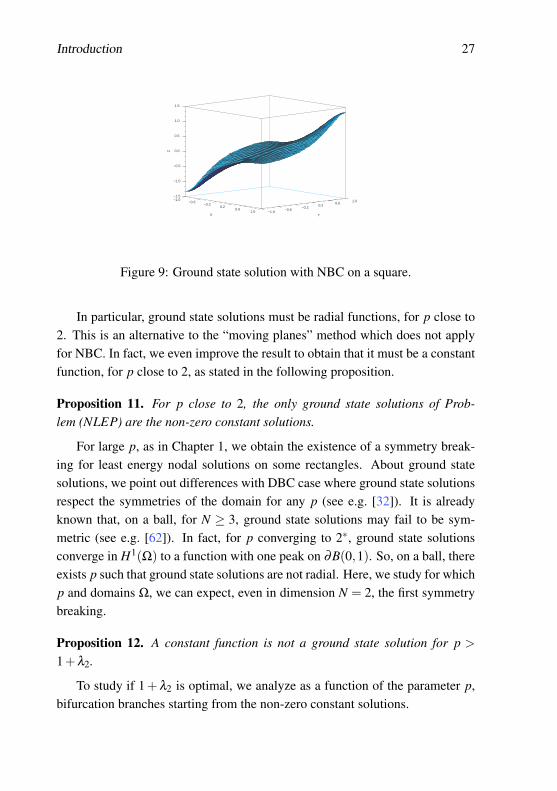
Figure 9: Ground state solution with NBC on a square.
In particular, ground state solutions must be radial functions, for p close to2. This is an alternative to the “moving planes” method which does not applyfor NBC. In fact, we even improve the result to obtain that it must be a constantfunction, for p close to 2, as stated in the following proposition.
Proposition 11. For p close to 2, the only ground state solutions of Prob-lem (NLEP) are the non-zero constant solutions.
For large p, as in Chapter 1, we obtain the existence of a symmetry break-ing for least energy nodal solutions on some rectangles. About ground statesolutions, we point out differences with DBC case where ground state solutionsrespect the symmetries of the domain for any p (see e.g. [32]). It is alreadyknown that, on a ball, for N ≥ 3, ground state solutions may fail to be sym-metric (see e.g. [62]). In fact, for p converging to 2∗, ground state solutionsconverge in H1(Ω) to a function with one peak on ∂B(0,1). So, on a ball, thereexists p such that ground state solutions are not radial. Here, we study for whichp and domains Ω, we can expect, even in dimension N = 2, the first symmetrybreaking.
Proposition 12. A constant function is not a ground state solution for p >
1+λ2.
To study if 1 + λ2 is optimal, we analyze as a function of the parameter p,bifurcation branches starting from the non-zero constant solutions.
28 Introduction
Theorem 13. • If dimEi is even (resp. odd), a sequence (resp. branch) ofsolutions starts from the non-zero constant solutions if and only if 2 <
p < 2∗ equals 1+λi, for any i≥ 2;
• on balls, if Ei does not contain non-zero radial functions (as e.g. wheni = 2), bifurcations are not radial;
• on balls, if Ei contains one non-zero radial function (e.g. if dimEi = 1),there exists at least one radial branch of solutions starting from the non-zero constant solutions.
On radial domains, let us just remark that, inspired by the paper [3] of A. Af-talion and F. Pacella, we also obtain that non-constant ground state solutionscannot be radial.
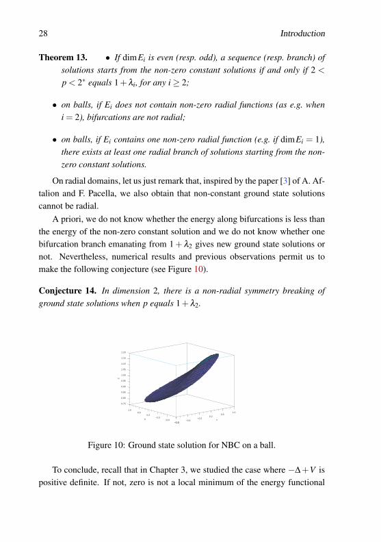
A priori, we do not know whether the energy along bifurcations is less thanthe energy of the non-zero constant solution and we do not know whether onebifurcation branch emanating from 1 + λ2 gives new ground state solutions ornot. Nevertheless, numerical results and previous observations permit us tomake the following conjecture (see Figure 10).
Conjecture 14. In dimension 2, there is a non-radial symmetry breaking ofground state solutions when p equals 1+λ2.
0.75
0.80
0.85
0.90
0.95
1.00
1.05
1.10
1.15
1.20
Z
−1.0−0.6
−0.20.2
0.61.0
Y−1.0
−0.6−0.2
0.20.6
1.0
X
Figure 10: Ground state solution for NBC on a ball.
To conclude, recall that in Chapter 3, we studied the case where −∆ +V ispositive definite. If not, zero is not a local minimum of the energy functional
Introduction 29
and so the problem does not respect a mountain pass geometry anymore. Nev-ertheless, P. H. Rabinowitz proved the existence of a ground state solution (seee.g. [61]). Recently, in 2009, A. Szulkin and T. Weth even obtained the exis-tence of ground state solutions if Ω = RN [64]. Let us just remark that, now,ground state solutions could be sign-changing.
Concerning symmetry results, this time, results obtained in Chapter 1 donot work in this case. So, in the last chapter, we focus on the existence of analgorithm to approach these solutions, we prove its convergence, we implementit and we make conjectures on the symmetries, at least when V is constant. Inthe classical case where the energy functional respects a mountain pass struc-ture, the mountain pass algorithm (MPA) can directly be used. This is a con-strained steepest descent method. It was introduced in 1993 by Y. S. Choi andP. J. McKenna [24] and approaches solutions with Morse index10 equals to 1(like the ground state solutions). Typically, the algorithm is working like this.
Algorithm 15. 1. Let u ∈ H10 (Ω) with energy functional E (u) strictly neg-
ative;
2. compute initial path: γi = iN u, i = 0, . . . ,N; n← 0;
3. compute un := γ j = argmaxE (γi) : i = 0, . . . ,N and improve the local-ization of the maximum of “E ([0,u])” by quadratic interpolation;
4. compute gn = ∇E (un): if ‖gn‖6 ε , then stop;else deform the path: move γ j in argmins≥0E (un− sgn), n← n + 1 andgo to step 3;
5. restart in step 2.
In 2001, J. Zhou and Y. Li [71, 72] proved the convergence, at least up to asubsequence, of a “variant” of MPA (see Introduction of Chapter 6 for details).
For sign-changing solutions, let us mention that the modified mountain passalgorithm (MMPA) has been proposed in 1997 by J. M. Neuberger [54] (seealso [25]). Based on the MPA, it allows to approach sign-changing solution butthe convergence of the algorithm is not proven for now. Here, we generalize the
10Number of descent directions for the second derivative of the energy functional.
30 Introduction
mountain pass algorithm to approach a non-zero solution even if −∆+V has anegative spectrum. We prove the convergence of the algorithm.
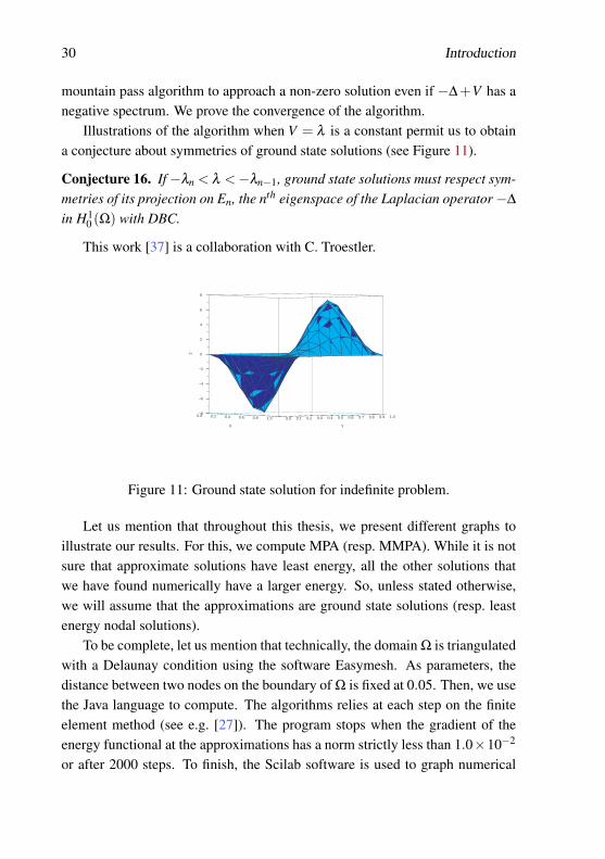
Illustrations of the algorithm when V = λ is a constant permit us to obtaina conjecture about symmetries of ground state solutions (see Figure 11).
Conjecture 16. If−λn < λ <−λn−1, ground state solutions must respect sym-metries of its projection on En, the nth eigenspace of the Laplacian operator−∆
in H10 (Ω) with DBC.
This work [37] is a collaboration with C. Troestler.
−8
−6
−4
−2
0
2
4
6
8
Z
0.0 0.1 0.2 0.3 0.4 0.5 0.6 0.7 0.8 0.9 1.0
Y
0.0 0.2 0.4 0.6 0.8 1.0
X
Figure 11: Ground state solution for indefinite problem.
Let us mention that throughout this thesis, we present different graphs toillustrate our results. For this, we compute MPA (resp. MMPA). While it is notsure that approximate solutions have least energy, all the other solutions thatwe have found numerically have a larger energy. So, unless stated otherwise,we will assume that the approximations are ground state solutions (resp. leastenergy nodal solutions).
To be complete, let us mention that technically, the domain Ω is triangulatedwith a Delaunay condition using the software Easymesh. As parameters, thedistance between two nodes on the boundary of Ω is fixed at 0.05. Then, we usethe Java language to compute. The algorithms relies at each step on the finiteelement method (see e.g. [27]). The program stops when the gradient of theenergy functional at the approximations has a norm strictly less than 1.0×10⁻²
or after 2000 steps. To finish, the Scilab software is used to graph numerical
Introduction 31
solutions. Readers can find more explainations and examples in [35] and canvisit the following web page11 to get a free access code.
11http://staff.umh.ac.be/Grumiau.Christopher/

32 Introduction
Chapter 1
Lane–Emden problem withDBC: symmetries of somevariational solutions
As mentioned in the Introduction, we work with the so-called Lane–EmdenProblem (LEP) with Dirichlet boundary conditions
−∆u = |u|p−2u, in Ω,
u = 0, on ∂Ω,(LEP)
where Ω is an open bounded connected domain in RN , N ≥ 2 and 2 < p < 2∗ :=2N
N−2 (+∞ if N = 2).The solutions are the critical points of the energy functional defined on the
Sobolev space1 H10 (Ω) and given by
12
∫Ω
|∇u|2− 1p
∫Ω
|u|p.
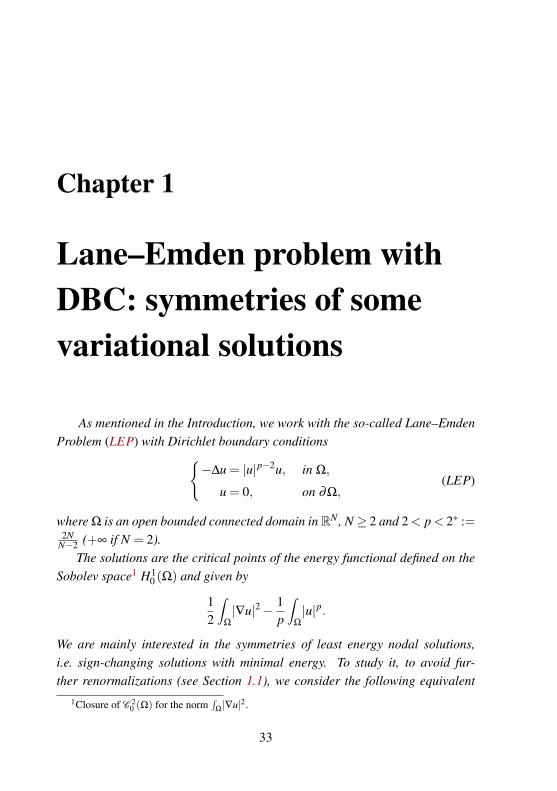
We are mainly interested in the symmetries of least energy nodal solutions,i.e. sign-changing solutions with minimal energy. To study it, to avoid fur-ther renormalizations (see Section 1.1), we consider the following equivalent
1Closure of C 20 (Ω) for the norm
∫Ω|∇u|2.
33
34 Chapter 1 — Lane–Emden problem with DBC
t∗u ∈Npu0
Ep
Figure 1.1: Nehari manifold.
Problem (Pp) −∆u = λ2|u|p−2u, in Ω,
u = 0, on ∂Ω,(Pp)
where λ2 is the second eigenvalue of −∆ in H10 (Ω) with DBC. We denote by
E2 the eigenspace related to λ2. Weak solutions of Problem (Pp) are criticalpoints of the energy functional Ep defined on the Sobolev space H1
0 (Ω) andgiven by
Ep(u) =12
∫Ω
|∇u|2− λ2
p
∫Ω
|u|p.
Let us remark that, by the regularity theory (see e.g. [19]), it is possible to provethat weak solutions are in fact classical ones; they belong to C 2
0 (Ω)∩C (Ω).Clearly u is a solution (resp. least energy nodal solution) of Problem (LEP)
if and only if λ1/(2−p)2 u is a solution (resp. l.e.n.s.) of Problem (Pp). So, this
rescaling does not change the symmetries of solutions.To start the study, let us explain the structure of the energy functional Ep.
The functional Ep is a C 2-functional. At u ∈H10 (Ω), the first Frechet derivative
of Ep at u in the direction v is given by
〈dEp(u),v〉=∫
Ω
∇u∇v−λ2
∫Ω
|u|p−2uv,
and the second one in the directions v and w reads
〈d2Ep(u),v,w〉=∫
Ω
∇v∇w− (p−1)λ2
∫Ω
|u|p−2vw.
Moreover, the Palais-Smale condition holds for Ep (see e.g. [35]), i.e. fromany sequence (un)n∈N ⊆ H1
0 (Ω), if Ep((un)n∈N) is bounded and if the gradient
35
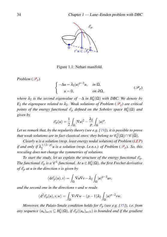
∇Ep(un) converges to zero then (un)n∈N converges up to a subsequence. Thisis a classical condition generally required to obtain existence and multiplic-ity results. Note that the constant zero function is clearly a critical point ofEp. Concerning non-zero critical points, seeking minima of Ep does not giveanything since Ep is not bounded from below. Nevertheless, we can obtain acharacterization of some non-zero critical points by defining the Nehari mani-fold Np (see Figure 1.1) and the nodal Nehari set Mp by
Np := u ∈H10 (Ω)\0 : 〈dEp(u),u〉= 0, Mp := u ∈H1
0 (Ω) : u± ∈Np,
where u+(x) := max(0,u(x)) and u−(x) := min(0,u(x)).The interest of Np comes from the fact that it contains all the non-zero cri-
tical points of Ep and that the functions in Np stay away from the zero function.This is a C 1-manifold. A function is a ground state solution of Problem (Pp)if and only if it minimizes Ep on Np. As the energy functional respects thePalais-Smale condition, it is possible to prove that these minima are achieved(see e.g. [6, 35]). From classical minimization arguments, we deduce that thesesolutions are one-signed functions: for any sign-changing solution u, Ep(u±) <
Ep(u) and u± ∈Np. If u ∈ H10 (Ω) then u ∈Np if and only if∫Ω
|∇u|2 = λ2
∫Ω
|u|p, (1.1)
which implies that(
12 −
1p
)‖u‖2 = Ep(u). An other interesting fact is that for
any u∈H10 (Ω)\0, there exists one and only one positive multiplicative factor
t∗ > 0 such that t∗u ∈Np, which gives a projection from H10 (Ω) \ 0 to Np.
We also have that t∗u is the unique local maximum of Ep in the direction u, i.e.Ep(t∗u) = maxt>0(Ep(tu)).
The interest of Mp comes from the fact that it contains all sign-changingcritical points of Ep. A function is said to be a least energy nodal solution ofProblem (Pp) if and only if it minimizes Ep on Mp. Let us just remark that,because the functions u 7→ u± are not C 1, Mp is not a C 1-manifold anymore.Nevertheless, it is possible to prove that these minima are achieved (see e.g. [23,35] or Section 3.2 for a proof for more general problems). Similar argumentsas before show that these solutions have two nodal domains, just as the secondeigenfunctions of −∆. If u ∈ H1
0 (Ω), u+ 6= 0 and u− 6= 0, then u ∈Mp if and
36 Chapter 1 — Lane–Emden problem with DBC
only if ∫Ω
|∇u+|2 = λ2
∫Ω
|u+|p and∫
Ω
|∇u−|2 = λ2
∫Ω
|u−|p. (1.2)
We can obtain a projection from H10 (Ω) restricted to the sign-changing func-
tions to Mp: at u, we consider the maximization of the energy function Ep onthe quarter of plane
αu+ +βu− : α ≥ 0, β ≥ 0
.
In this first chapter, with the aim to obtain further symmetry results, we startby studying the asymptotic behavior of a family of least energy nodal solutions(up)p>2. As p→ 2, in Section 1.1, our results basically show that, for gen-eral domains Ω, (up)p>2 is bounded in H1
0 (Ω) and stays away from 0. This istrue thanks to the rescaling that was performed to obtain the equation (Pp).Moreover, we give a variational characterization of accumulation points of up.
In Section 1.2, inspired by the work of D. Smets, J. Su and M. Willem [63]which studied, for the Hénon problem (i.e. −∆u = |x|α up), the radiality ofground state solutions when p is close to 2, we use the boundedness to applythe following implicit function theorem and conclude symmetries in the casewhere dimE2 = 1 (like rectangles). Similar arguments have been also usedin [28, 46],... Let us recall the implicit function theorem for the reader’s conve-nience.
Implicit Function Theorem. Let ψ : A×H→H : (λ ,u) 7→ ψ(λ ,u) a C 1(A×H,H) function where A is in RN and H is a Banach space. Assume thatψ(λ0,u0) = 0 and ∂uψ(λ0,u0) is invertible.Then, there exists a neighbourhood B := B(λ0,r)× B(u0,R) of (λ0,u0) andγ ∈ C 1(B(λ0,r),B(u0,R)) such that
∀(λ ,u) ∈ B, ψ(λ ,u) = 0 if and only if u = γ(λ ).
When dimE2 6= 1, we cannot use directly the implicit function theorem. Nev-ertheless, on radial domains, as we are able to show that the degeneracy of thesecond eigenspace is solely due to the invariance of (Pp) under the group ro-tations (see Proposition 1.3.1), we are able to use the implicit function theoremby defining a “good” subspace of H1
0 (Ω). That enables us to obtain that leastenergy nodal solutions are even with respect to N− 1 independent directions
1.1 — Asymptotic behavior 37
and odd with respect to the orthogonal one. Moreover, we establish uniqueness(up to the action of the group of rotations). This part is explained in Section 1.3.
In Section 1.4, we deal with general domains. We prove that a boundedfamily of solutions, not necessarily ground state or least energy nodal solutions,can be distinguished by their projections on the second eigenspace: for everyM > 0, there exists p > 2 such that, for every α ∈ E2 \0, for every p ∈ (2, p),Problem (Pp) has at most one solution in the set u ∈ B(0,M) | PE2u = α.
This uniqueness property immediately implies partial symmetries if all thesecond eigenfunctions enjoy some common symmetry (like for the square wheresecond eigenfunctions are odd with respect to the barycenter).
In Section 1.4.3, using the variational characterization of accumulationpoints of up, we obtain a more precise symmetry result on the square. Weconjecture that least energy nodal solutions are symmetric with respect to adiagonal and antisymmetric in the orthogonal direction.
In Section 1.5, we discuss about an example of symmetry breaking: thereexists a rectangle such that any least energy nodal solutions of Problem (Pp)is neither symmetric nor antisymmetric with respect to the medians.
The part related to the “implicit function theorem” is inspired by the pa-per [39] written in collaboration with C. Troestler. The part on “general do-mains” is inspired by the paper [14] written in collaboration with D. Bon-heure, V. Bouchez and J. Van Schaftingen. In this thesis, we will use classi-cal tools related to the functional analysis (the Lebesgue’s dominated conver-gence theorem, closed graph theorem, Fredholm alternative,...). Concerningthe Sobolev space theory, the Sobolev’s embeddings, the Rellich’s embeddingand the Poincaré’s inequalities are mentioned in the Appendix A. Most of themhave also been studied in the Master’s thesis [35]. Readers can also referto [49, 55, 70].
1.1 Asymptotic behavior
Let us fix (up)p>2 a family of least energy nodal solutions of the Problem (Pp).We prove that (up)p>2 is bounded in H1
0 (Ω) and stays away from 0.
38 Chapter 1 — Lane–Emden problem with DBC
1.1.1 Upper bound
We prove it by using two different ways. The first one (see Proposition 1.1.2),is more classical but the bound is less precise than the second one (see Proposi-tion 1.1.3). Let us fix a non-zero second eigenfunction e2 of −∆.
Lemma 1.1.1. For 2 < r < 2∗, the quantities sup2<p<r t+p and sup2<p<r t−p arefinite, where t+p and t−p are the unique positive real numbers such that t+p e+
2 +t−p e−2 ∈Mp.
Proof. Let us fix r ∈ (2,2∗) and p ∈ (2,r). Since (t±p )2‖e±2 ‖2 = (t±p )pλ2‖e±2 ‖pp,
we have
t±p =(‖e±2 ‖2
λ2‖e±2 ‖pp
) 1p−2
> 0.
It is enough to show that t±p converges, as p→ 2. We have
limp→2
ln(‖e±2 ‖2
2
λ2‖e±2 ‖pp
) 1p−2
= limp→2
1p−2
(ln‖e±2 ‖
2− ln(λ2‖e±2 ‖pp)).
As e2 is a second eigenfunction of−∆, we have λ2‖e±2 ‖22 = ‖e±2 ‖2. By denoting
Ω± := x ∈Ω : e±2 6= 0, we apply the l’Hôpital’s rule to obtain
limp→2
ln(‖e±2 ‖2)− ln(λ2‖e±2 ‖pp)
p−2= lim
p→2
−∫
Ω± |e±2 |p ln |e±2 |∫
Ω± |e±2 |p
=−∫
Ω± |e±2 |2 ln |e±2 |∫
Ω± |e2|2
so that
limp→2
t±p = exp−∫
Ω± |e±2 |2 ln |e±2 |∫
Ω± |e±2 |2
.
Proposition 1.1.2. The family (up)p>2 is bounded in H10 (Ω).
Proof. Let us define t±p as in Lemma 1.1.1. As up belongs to the nodal Nehariset Mp, ‖up‖2 = λ2‖up‖p
p. On one hand, as the supports of e+2 and e−2 are
disjoint, we have that(12− 1
p
)‖up‖2 = Ep(up) = inf
u∈MpEp(u)≤ Ep(t+p e+
2 + t−p e−2 )
= Ep(t+p e+2 )+Ep(t−p e−2 ).
1.1 — Asymptotic behavior 39
On the other hand, as t+p e+2 ∈Np, we have
Ep(t+p e+2 ) =
(12− 1
p
)(t+p )2‖e+
2 ‖2
and analogously for Ep(t−p e−2 ). So, we obtain
‖up‖22 ≤ (t+p )2‖e+
2 ‖2 +(t−p )2‖e−2 ‖
2.
From the uniform boundedness of t+p and t−p (see Lemma 1.1.1), the claim fol-lows.
For the second approach, we obtain the upper bound by a suitable choice oftest functions. In the proof, we work with the following reduced functional
E∗ : E2→ R : u 7→ λ2
2
∫Ω
u2−u2 logu2 (1.3)
(where t2 log t2 is extended continuously by 0 at t = 0). The critical points ofE∗ are the functions u∗ such that
∀v ∈ E2,∫
Ω
vu∗ logu2∗ = 0. (1.4)
Any non-trivial critical points again belong to the reduced Nehari manifold
N∗ := u ∈ E2 \0 : 〈dE∗(u),u〉= 0. (1.5)
This manifold is compact and such that u ∈N∗ if and only if∫Ω
u2 logu2 = 0,
or equivalently if and only if
E∗(u) =λ2
2‖u‖2
2.
Observe that, for any u ∈ E2 \ 0, there exists again a unique constant t∗u > 0such that t∗u u ∈N∗.

40 Chapter 1 — Lane–Emden problem with DBC
Proposition 1.1.3. Let (up)p>2 be a family of least energy nodal solutions ofProblem (Pp). Then we have
limsupp→2
‖up‖2 = limsupp→2
(Ep(up)12 −
1p
)6 ‖u∗‖2,
where u∗ ∈ E2 minimizes the reduced functional E∗ on the reduced Nehari man-ifold N∗.
Proof. Let w ∈ H10 (Ω) be a solution of the problem−∆w−λ2w = λ2u∗ log |u∗|, in Ω,
PE2w = 0,(1.6)
where PE2 denotes the orthogonal projection on E2 in H10 (Ω). Since u∗ verifies
the equation (1.4), by the Fredholm alternative, w is well-defined. Set
vp := u∗+(p−2)w
and
vp := t+p v+p + t−p v−p , where t±p =
(‖v±p ‖2
λ2‖v±p ‖pp
) 1p−2
,
so that vp ∈Mp. We claim that t±p → 1. By definition of vp, we have
‖v±p ‖2 =∫
Ω
∇vp ·∇v±p
=∫
Ω
(λ2u∗+λ2(p−2)w+λ2(p−2)u∗ log |u∗|)v±p
= λ2
∫Ω
(vp +(p−2)u∗ log |u∗|)v±p
= λ2
∫Ω
|vp|p−2vpv±p
+λ2(p−2)(∫
Ω
vp−|vp|p−2vp
p−2v±p +
∫Ω
u∗ log |u∗|v±p)
.
1.1 — Asymptotic behavior 41
Since we have ∣∣∣∣ t−|t|p−2tp−2
∣∣∣∣= 1p−2
∫ p
2
∣∣t log |t|∣∣ |t|q−2 dq
≤∣∣log |t|
∣∣(|t|+ |t|p−1)≤ 1
s
(|t|1−s + |t|p−1+s) ,
where s > 0 has been choosed small enough, considering results A.1 and A.2and applying the Lebesgue’s dominated convergence theorem, we infer that
limp→2
∫Ω
(vp−|vp|p−2vp
p−2+u∗ log |u∗|
)v±p = 0.
Therefore, we deduce that
‖v±p ‖2 = λ2
∫Ω
|v±p |p +o(p−2), (1.7)
so that limp→2 t±p = 1. At last, since
Ep(up)≤ Ep(vp)
and (12− 1
p
)−1
Ep(vp) = ‖∇vp‖2 = ‖u∗‖2 +o(1),
the conclusion follows easily.
Remark 1.1.4. Geometrically, this can be pictured as follows: the natural pro-jection of u∗ on the nodal Nehari set is far from u∗, but u∗ gets nearer to theNehari manifold as p→ 2.
1.1.2 Lower bound
In this part, we give a lower bound for a family of least energy nodal solutions(up)p>2.
Lemma 1.1.5. For any p ∈ (2,2∗) and u ∈ H10 (Ω)\0 such that u+ 6= 0 and
u− 6= 0, there exist t+ > 0 and t− > 0 such that t+u+ + t−u− belongs to Np andis orthogonal to e1 in L2(Ω), where e1 > 0 is a first eigenfunction of −∆.
42 Chapter 1 — Lane–Emden problem with DBC
Proof. We consider the line segment
T : [0,1]→ H10 (Ω)\0 : α 7→ (1−α)u+ +αu−.
We project it on Np: for all α ∈ (0,1), there exists a unique tα > 0 such thattα T (α) ∈ Np. For α = 0, we have
∫Ω
tα u+e1 > 0 and, for α = 1, we have∫Ω
tα u−e1 < 0. The continuity implies the existence of α∗ ∈ (0,1) such that∫Ω
tα∗T (α∗)e1 = 0 and tα∗T (α∗) ∈ Np. We just set t+ := tα∗(1− α∗) andt− := tα∗α∗ to conclude.
Proposition 1.1.6. All accumulation points of up as p→ 2 are non-zero func-tions.
Proof. By Lemma 1.1.5, for all p ∈ (2,2∗), there exist t±p > 0 such that vp :=t+p u+
p + t−p u−p belongs to Np and is orthogonal to e1 in L2(Ω).We claim that ‖vp‖p 6 ‖up‖p. As up ∈Mp, u+
p ∈Np maximizes the energyfunctional Ep in the direction of u+
p and, similarly, u−p ∈Np maximizes Ep inthe direction of u−p . As the energy is the sum of the energy of the positive andnegative parts, up maximizes the energy in the cone K := t+u+
p + t−u−p : t+ >
0 and t− > 0. Since vp ∈Np implies λ2( 1
2 −1p
)‖vp‖p
p = Ep(vp) and given thatvp ∈Np∩K, we deduce
λ2
(12− 1
p
)‖vp‖p
p = Ep(vp)6 Ep(up) = λ2
(12− 1
p
)‖up‖p
p.
Thus the claim is proved.Let us now prove that vp stays away from zero. By Hölder inequality, we
have‖vp‖2
p 6 ‖vp‖2−2λ
2 ‖vp‖2λ2∗ ,
where λ := 2∗2∗−2
p−2p . (In dimension 2, 2∗ = +∞. In this case, we can replace
2∗ by a sufficiently large q in the last inequality and use the same argument asbelow.) As vp is orthogonal to e1 in L2(Ω), λ2
∫Ω
v2p 6 ‖vp‖2. By Sobolev’s
embedding theorem A.6, there exists a constant S > 0 such that
‖vp‖2p 6
(λ−12 ‖vp‖2)1−λ (S−1‖vp‖2)λ = λ
−12 ‖vp‖2 (
λ2S−1)λ.
As vp belongs to Np, ‖vp‖2 = λ2‖vp‖pp and so
‖vp‖2p 6 ‖vp‖p
p(S−1
λ2)λ
1.1 — Asymptotic behavior 43
or, equivalently,
‖vp‖p >(Sλ−12)λ/(p−2) =
(Sλ−12) 2∗
2∗−21p .
Therefore, if u∗ is the weak limit of a sequence (upn)n∈N in H10 (Ω) for some
sequence pn −→ 2, by using Rellich’s embedding theorem A.7,
‖u∗‖2 = limn→∞‖upn‖pn > liminf
n→∞‖vpn‖pn > 0.
As ‖up‖2 = λ2‖up‖pp on Np, let us remark that we have that our family is
also staying away from zero for H10 -norm.
1.1.3 Conclusion: limit equation and variational characteri-zation
We consider a weak accumulation point u∗ of a bounded family (up)p>2 of so-lutions for Problem (Pp). We prove that those functions verify a limit equation.
Lemma 1.1.7. Let (up)p>2 be a bounded family of solutions for Problem (Pp).If upn u∗ in H1
0 (Ω) for some sequence pn→ 2, then u∗ solves−∆u∗ = λ2u∗, in Ω,
u∗ = 0, on ∂Ω,∫Ω
u∗ log |u∗|v = 0, ∀v ∈ E2.
Proof. Let v ∈ H10 (Ω). By Rellich’s embedding theorem and Lebesgue’s dom-
inated convergence theorem, we deduce that
|upn |pn−2upn → u∗ in L2(Ω),
so that ∫Ω
∇u∗ ·∇v = limn→∞
∫Ω
∇upn ·∇v
= limn→∞
λ2
∫Ω
|upn |pn−2upnv
= λ2
∫Ω
u∗v.
44 Chapter 1 — Lane–Emden problem with DBC
Hence, u∗ ∈ E2. To prove the last equality, taking v ∈ E2 and multiplying theequation in Problem (Pp) by v lead to∫
Ω
(|upn |pn−2upn −upn)v = 0. (1.8)
Arguing as in Proposition 1.1.3, we conclude, using Lebesgue’s dominated con-vergence theorem and equation (1.7), that
limn→∞
∫Ω
(|upn |pn−2upn −upn)vpn−2
=∫
Ω
u∗ log |u∗|v.
Taking (1.8) into account, this completes the proof.
Bringing together the previous lemmas, we now deduce a variational char-acterization for u∗.
Theorem 1.1.8. Let (up)p>2 be a family of least energy nodal solutions forProblem (Pp). If upn u∗ in H1
0 (Ω) for some sequence pn→ 2, then upn → u∗in H1
0 (Ω)\0, where u∗ satisfies−∆u∗ = λ2u∗, in Ω,
u∗ = 0, on ∂Ω,
and
E∗(u∗) = c := infE∗(u) : u ∈ E2 \0,〈dE∗(u),u〉= 0= infN∗
E∗.
Proof. By Lemma 1.1.7, u∗ ∈E2. Observe that, as E∗(u) = 12‖u‖
2 when u∈N∗,
inf‖u‖2 : u ∈ E2 \0,
∫Ω
u2 logu2 = 0
= 2c.
Applying successively Proposition 1.1.3, the weak lower semi-continuity of thenorm and Lemma 1.1.7, we deduce that
2c = limsupn→∞
‖upn‖2 > liminfn→∞
‖upn‖2 > ‖u∗‖2 > 2c.
Hence, we conclude that limn→∞‖upn‖2 = ‖u∗‖2 = 2c. This also implies imme-diately the strong convergence of the sequence (upn)n∈N.
1.2 — Nondegenerate case: dimE2 = 1 45
1.2 Nondegenerate case: dimE2 = 1
As we now know that a family of least energy nodal solutions (up)p>2 for Prob-lem (Pp) is bounded in H1
0 (Ω) and stays away from the zero function, we noware able to deduce some symmetries of up, at least in the case where dimE2 = 1and for p close to 2. The main idea is to apply the implicit function theorem(see page 34). Let us fix e2 ∈ E2 such that ‖e2‖= 1.
1.2.1 Method based on the implicit function theorem
Lemma 1.2.1. In dimension N > 2, in H10 (Ω)×R, Problem (1.9)
−∆u = λ |u|p−2u, in Ω,
u = 0, on ∂Ω,
‖u‖= 1,
(1.9)
possesses a single curve of solutions p 7→ (p, up,λ∗p ) defined for 2 < p close
to 2 and starting from (2,e2,λ2). It also possesses a single curve of solutionsstarting from (2,−e2,λ2) which is given by p 7→ (p,−up,λ
∗p ) .
Proof. Let us define
ψ : (2,2∗)×H10 (Ω)×R→ H1
0 (Ω)×R
(p,u,λ ) 7→(u−λ (−∆)−1(|u|p−2u),‖u‖2−1
).
The first component is the H10 -gradient of the following energy functional
Ep,λ : H10 (Ω)→ R : u 7→ 1
2‖u‖2− λ
p‖u‖p
p .
The existence and local uniqueness of a branch emanating from (2,e2,λ2)follows from the implicit function theorem and the closed graph theorem if weprove that the derivative of E with respect to (u,λ ) at the point (2,e2,λ2) isbijective on H1
0 (Ω)×R. We have,
∂(u,λ )ψ(2,e2,λ2)(v, t)
=(
v−λ2(−∆)−1v− t(−∆)−1e2, 2∫
Ω
∇e2∇v)
. (1.10)
46 Chapter 1 — Lane–Emden problem with DBC
For the injectivity, let us start by showing that ∂(u,λ )ψ(2,e2,λ2)(v, t) = 0 if andonly if
v−λ2(−∆)−1v = 0,
t = 0,
v is orthogonal to e2 in H10 (Ω).
(1.11)
It is clear that (1.11) is sufficient. For its necessity, remark that the nullity ofsecond component of (1.10) implies that e2 is orthogonal to v in H1
0 (Ω) andthus also in L2(Ω) because e2 is an eigenfunction. Taking the L2-inner productof the first component of (1.10) with e2 yields t = 0, hence the equivalence iscomplete. Now, the only solution of (1.11) is (v, t) = (0,0) because the firstequation and the dimension 1 of E2 imply that v = αe2, for some α ∈ R. Thethird property implies v = 0. This concludes the proof of the injectivity of∂(u,λ )ψ(2,e2,λ2).
Let us now show that, for any (w,s) ∈ H10 (Ω)×R, the equation
∂(u,λ )ψ(2,e2,λ2)(v, t) = (w,s)
always possesses at least one solution (v, t) ∈ H10 (Ω)×R. One can write w =
we2 + w for some w ∈ R and w orthogonal to e2 in H10 (Ω). Similarly, one can
decompose v = ve2 + v. Arguing as for the first part, the equation can be writtenv−λ2(−∆)−1v = w,
t = λ2w,
v = s/2.
(1.12)
By the principle of symmetric criticality, the solution v is the minimizer of thefunctional
E⊥2 → R : v 7→∫
Ω
|∇v|2−λ2|v|2−∫
Ω
∇w∇v.
This concludes the proof that ∂(u,λ )ψ(2,e2,λ2) is onto and thus of the existenceand uniqueness of the branch emanating from (2,e2,λ2).
It is clear that p 7→ (p,−u∗p,λ∗p ) is a branch emanating from (2,−e2,λ2)
and, using as above the implicit function theorem at that point, we know it isthe only one.
We deduce now some symmetries when dimE2 = 1.
1.2 — Nondegenerate case: dimE2 = 1 47
Theorem 1.2.2. Assume that λ2 is simple. Then, for p close to 2 and anyreflection R such that R(Ω) = Ω, least energy nodal solutions of Problem (Pp)respect the symmetries or antisymmetries of e2 with respect to R. Moreover,for p close to 2, least energy nodal solution of Problem (Pp) is unique up tosymmetries of the domain and multiplicative factor of value −1.
Proof. Let (up)p>2 be a family of solutions of Problem (Pp). On one hand, forany sequence pn→ 2, there exists a subsequence, still denoted pn, such that upn
weakly converges in H10 (Ω) to some u∗ = αe2 ∈ E2 \0 (thanks to 1.1.8).
On the other hand, notice that up is a solution of Problem (Pp) if and only if(up/‖up‖, λ2‖up‖p−2
)is a solution of (1.9). Because (upn)n∈N stays bounded
away from 0, one has(upn
‖upn‖,λ2‖upn‖pn−2
)−→n
(sign(α)e2,λ2
).
Then, when pn is close enough to 2, Lemma 1.2.1 implies that
upn
‖upn‖= sign(α)u∗pn .
Hence, this claimed uniqueness of up up to its sign. Let us define the reflection Rsuch that R(Ω) = Ω. We prove that upn respects symmetries of e2 with respect toR. W.l.o.g., assume that e2 is odd (resp. even) with respect to R (as dimE2 = 1,we are sure that e2 is odd or even with respect to R). To show the oddness (resp.evenness) of upn , let us consider u′pn the anti-symmetric (resp. symmetric) ofupn with respect to R defined by u′pn := ∓upn(x− 2(x.R)R) where x.R denotesthe inner product in RN . Because e2 is odd (resp. even) with respect to R,u′pn → αe2 with the same α as for u∗. Arguing as before, we conclude that
upn
‖upn‖= sign(α)u∗pn =
u′pn
‖u′pn‖
and therefore that upn is odd (resp. even) with respect to R.
1.2.2 Example: the rectangle
As an example, we immediately have that, on rectangles, least energy nodalsolutions are odd with respect to the small median and even with respect to
48 Chapter 1 — Lane–Emden problem with DBC
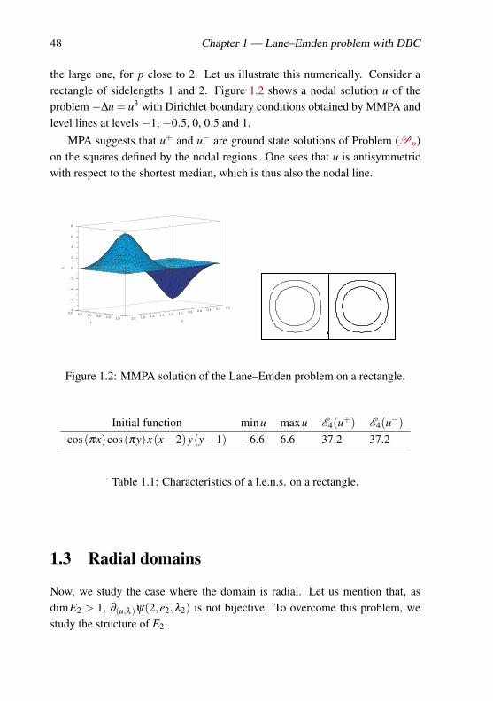
the large one, for p close to 2. Let us illustrate this numerically. Consider arectangle of sidelengths 1 and 2. Figure 1.2 shows a nodal solution u of theproblem −∆u = u3 with Dirichlet boundary conditions obtained by MMPA andlevel lines at levels −1, −0.5, 0, 0.5 and 1.
MPA suggests that u+ and u− are ground state solutions of Problem (Pp)on the squares defined by the nodal regions. One sees that u is antisymmetricwith respect to the shortest median, which is thus also the nodal line.
−8
−6
−4
−2
0
2
4
6
8
Z
0.00.20.40.60.81.01.21.41.61.82.0X
0.0 0.2 0.4 0.6 0.8 1.0Y
Figure 1.2: MMPA solution of the Lane–Emden problem on a rectangle.
Initial function minu maxu E4(u+) E4(u−)cos(πx)cos(πy)x(x−2)y(y−1) −6.6 6.6 37.2 37.2
Table 1.1: Characteristics of a l.e.n.s. on a rectangle.
1.3 Radial domains
Now, we study the case where the domain is radial. Let us mention that, asdimE2 > 1, ∂(u,λ )ψ(2,e2,λ2) is not bijective. To overcome this problem, westudy the structure of E2.
1.3 — Radial domains 49
1.3.1 Study of E2
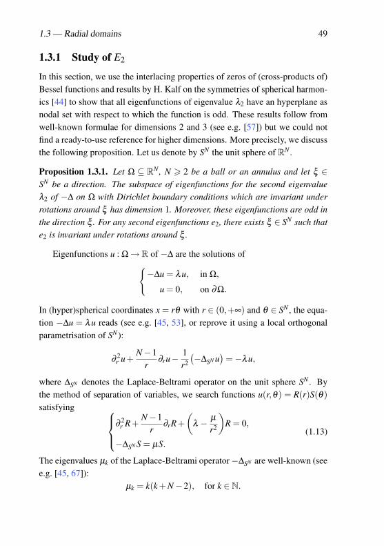
In this section, we use the interlacing properties of zeros of (cross-products of)Bessel functions and results by H. Kalf on the symmetries of spherical harmon-ics [44] to show that all eigenfunctions of eigenvalue λ2 have an hyperplane asnodal set with respect to which the function is odd. These results follow fromwell-known formulae for dimensions 2 and 3 (see e.g. [57]) but we could notfind a ready-to-use reference for higher dimensions. More precisely, we discussthe following proposition. Let us denote by SN the unit sphere of RN .
Proposition 1.3.1. Let Ω ⊆ RN , N > 2 be a ball or an annulus and let ξ ∈SN be a direction. The subspace of eigenfunctions for the second eigenvalueλ2 of −∆ on Ω with Dirichlet boundary conditions which are invariant underrotations around ξ has dimension 1. Moreover, these eigenfunctions are odd inthe direction ξ . For any second eigenfunctions e2, there exists ξ ∈ SN such thate2 is invariant under rotations around ξ .
Eigenfunctions u : Ω→ R of −∆ are the solutions of−∆u = λu, in Ω,
u = 0, on ∂Ω.
In (hyper)spherical coordinates x = rθ with r ∈ (0,+∞) and θ ∈ SN , the equa-tion −∆u = λu reads (see e.g. [45, 53], or reprove it using a local orthogonalparametrisation of SN):
∂2r u+
N−1r
∂ru−1r2
(−∆SN u
)=−λu,
where ∆SN denotes the Laplace-Beltrami operator on the unit sphere SN . Bythe method of separation of variables, we search functions u(r,θ) = R(r)S(θ)satisfying ∂
2r R+
N−1r
∂rR+(
λ − µ
r2
)R = 0,
−∆SN S = µS.
(1.13)
The eigenvalues µk of the Laplace-Beltrami operator−∆SN are well-known (seee.g. [45, 67]):
µk = k(k +N−2), for k ∈ N.
50 Chapter 1 — Lane–Emden problem with DBC
The corresponding eigenfunctions Sk are called spherical harmonics. Theseare restrictions to the unit sphere (S = PSN ) of homogeneous polynomials P :RN → R satisfying ∆P = 0 in RN . The eigenfunctions of eigenvalue µk arethe restrictions of the homogeneous polynomials of degree k among those [53,p. 39].
In order for R(r) =: r−N−2
2 B(√
λ r) to be solution of the first equation ofthe system (1.13) with µ = µk, it is necessary and sufficient that the functions 7→ B(s) satisfies
∂2s B+
1s
∂sB+(
1− ν2
s2
)B = 0, (1.14)
where ν2 := µk + (N−2)2
4 =(k + N−2
2
)2. Solutions of equation (1.14) are linear
combinations of the Bessel functions of the first kind
Jν(s) :=( s
2
)ν +∞
∑k=0
(−1)ks2k
22kΓ(k +1)Γ(ν + k +1)
where, for any c > 0, Γ(c) :=∫ +∞
0 xc−1e−x dx denotes the gamma functions, andof the second kind
Yν(s) := limz→ν
Jz(s)cos(zπ)− J−z(s)sin(zπ)
.
It is easy to prove by induction that Γ(n) = (n−1)! for all n ∈ N.Therefore, the solutions of the first equation of (1.13) with µ = µk are
R(r) = r−N−2
2
(aJν
(√λ r)+bYν
(√λ r))
, a,b ∈ R, (1.15)
where ν = k + N−22 .
Let us now distinguish two cases.
If Ω is a ball—which can be assumed to be of radius one without loss ofgenerality—, the function Yν cannot appear in (1.15) because limr→0 Yν(r) =−∞ and image at 0 must be finite. Imposing the Dirichlet boundary conditions,we obtain that the eigenvalue λ must be the square of a positive root of Jν . If theradius of Ω goes to +∞, let us remark that eigenvalues go to 0. As is customary,let us denote 0 < jν ,1 < jν ,2 < · · · the infinitely many positive roots of Jν . The
1.3 — Radial domains 51
J0
J1J2 J3 J4 J5 J6
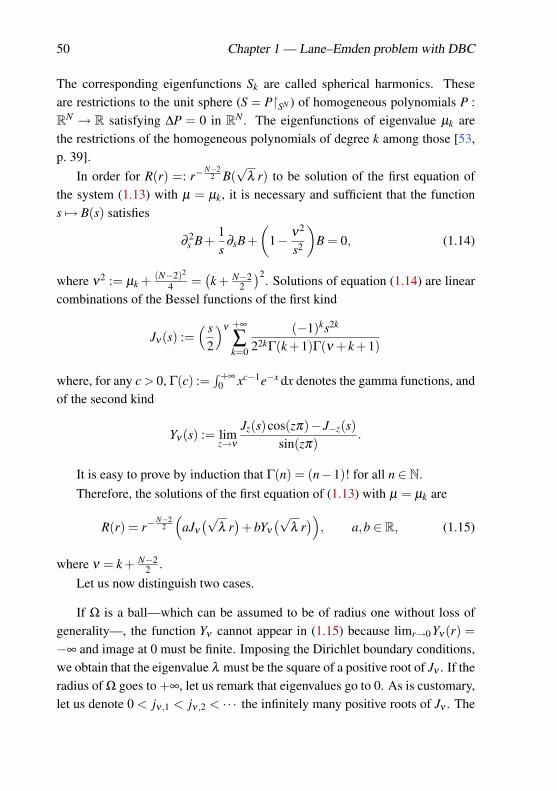
Figure 1.3: Bessel functions.
interlacing property of the roots (see e.g. M. Abramowitz and A. Segun [1,§ 9.5.2, p. 370]) says,
∀ν > 0, jν ,1 < jν+1,1 < jν ,2 < jν+1,2 < · · · (1.16)
The figure 1.3 illustrates this fact for the first few values of ν . So, in partic-ular, we obtain that j2
N−22 ,1
is the first eigenvalue of −∆ and j2N2 ,1
its second.
Therefore, the eigenfunctions for the second eigenvalue of −∆ are given by
r−N−2
2 JN/2(√
λ r)S(θ) with λ = j2
N2 ,1,
where S is a spherical harmonic of eigenvalue µ1.To conclude it suffices to use the fact that, for all directions ξ ∈ SN and
k ∈ N, there exists exactly one (apart from a multiplicative constant) homoge-neous polynomial P of degree k such that ∆P = 0 and is invariant under rotationsaround ξ (see e.g. [44, 53]). Therefore, there exists one and only one spheri-cal harmonic of eigenvalue µ1 that is invariant under rotations around a givendirection ξ . Moreover, this spherical harmonic is the restriction to the sphereof an homogeneous polynomial of degree 1 — i.e. a linear functional — and isconsequently odd in the direction ξ .
52 Chapter 1 — Lane–Emden problem with DBC
Now let us turn to the second case where Ω is an annulus. Without loss ofgenerality, one can assume that its internal radius is 1 and its external radius isρ ∈ (1,+∞). Imposing the Dirichlet boundary conditions on (1.15) leads to thesystem
aJν(√
λ )+bYν(√
λ ) = 0,
aJν(√
λρ)+bYν(√
λρ) = 0.
A non-trivial solution (a,b) of this system exists if and only if√
λ is a root of the function s 7→ Jν(s)Yν(sρ)−Yν(s)Jν(sρ).
It is known that this function possesses infinitely many positive zeros that wewill note 0 < χν ,1 < χν ,2 < · · · Again an interlacing theorem for these zerosholds [16, p. 1736]: for all ν > 0, χν ,1 < χν+1,1 < χν ,2 < χν+1,2 < · · · Asbefore, we deduce that the first eigenvalue happens for k = 0 (constant sphericalharmonic) and ν = (N− 2)/2, while the second is when k = 1 and ν = N/2.We then conclude in the same way as for the ball.
1.3.2 Method based on the “Radial IFT”
To be able to apply the implicit function theorem (see page 34), let us fix a direc-tion ξ ∈ SN . In the Introduction, we mentioned that, in 2005, T. Bartsch, T. Wethand M. Willem [8] proved that, on radial domains, least energy nodal solutionsrespect a Schwarz foliated symmetry. So, they are rotationally invariant arounda direction. Without loss of generality, up to rotations, we can assume that leastenergy nodal solutions are rotationally invariant around ξ . In Section 1.3.1,we obtained that the dimension of the space E2 ∩Fix(G), where Fix(G) is thespace H1
0 (Ω) restricted to the functions rotationally invariant around ξ , equals1. Moreover, these functions are odd in direction ξ . If we denote by e2 a func-tion in E2∩Fix(G), we obtain the following result.
Proposition 1.3.2. All weak accumulation points of the family (up)p>2 as p→ 2are invariant under rotations leaving ξ fixed and have the form αe2 for someα ∈ R\0.
By working exactly in the same way as in Section 1.2.1 but by using theimplicit function theorem (see page 34) on Fix(G) (instead of all H1
0 (Ω)), wedirectly obtain the following result.
1.3 — Radial domains 53
Theorem 1.3.3. Assume that Ω is a ball or an annulus. Then, for p close to2, least energy nodal solutions of Problem (Pp) are radially symmetric withrespect to N− 1 independent directions and antisymmetric with respect to theorthogonal one. Moreover, for p close to 2, least energy nodal solution is uniqueup to rotations and multiplicative factor of value −1.
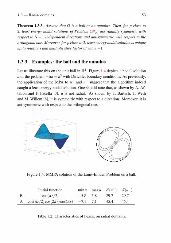
1.3.3 Examples: the ball and the annulus
Let us illustrate this on the unit ball in R2. Figure 1.4 depicts a nodal solutionu of the problem −∆u = u3 with Dirichlet boundary conditions. As previously,the application of the MPA to u+ and u− suggest that the algorithm indeedcaught a least energy nodal solution. One should note that, as shown by A. Af-talion and F. Pacella [3], u is not radial. As shown by T. Bartsch, T. Wethand M. Willem [8], it is symmetric with respect to a direction. Moreover, it isantisymmetric with respect to the orthogonal one.
−6
−4
−2
0
2
4
6
Z
−1.0−0.6
−0.20.2
0.61.0 X
−1.0−0.6
−0.20.2
0.61.0Y
Figure 1.4: MMPA solution of the Lane–Emden Problem on a ball.
Initial function minu maxu E (u+) E (u−)B cos(πr/2) −5.8 5.8 29.7 29.7A cos(πr/2)cos(2πr)cos(πr) −7.1 7.1 45.4 45.4
Table 1.2: Characteristics of l.e.n.s. on radial domains.
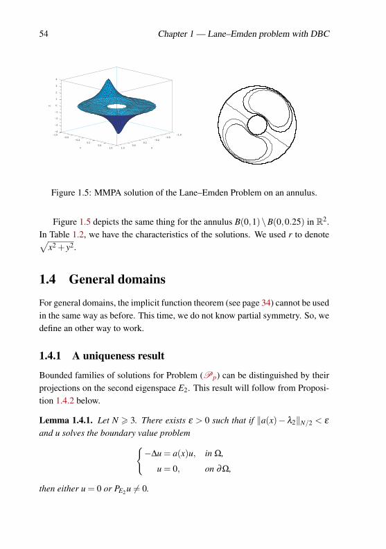
54 Chapter 1 — Lane–Emden problem with DBC
−4
−3
−2
−1
0
1
2
3
4
Z
−1.0−0.6
−0.20.2
0.61.0 X
−1.0−0.6
−0.20.2
0.61.0Y
Figure 1.5: MMPA solution of the Lane–Emden Problem on an annulus.
Figure 1.5 depicts the same thing for the annulus B(0,1)\B(0,0.25) in R2.In Table 1.2, we have the characteristics of the solutions. We used r to denote√
x2 + y2.
1.4 General domains
For general domains, the implicit function theorem (see page 34) cannot be usedin the same way as before. This time, we do not know partial symmetry. So, wedefine an other way to work.
1.4.1 A uniqueness result
Bounded families of solutions for Problem (Pp) can be distinguished by theirprojections on the second eigenspace E2. This result will follow from Proposi-tion 1.4.2 below.
Lemma 1.4.1. Let N > 3. There exists ε > 0 such that if ‖a(x)−λ2‖N/2 < ε
and u solves the boundary value problem−∆u = a(x)u, in Ω,
u = 0, on ∂Ω,
then either u = 0 or PE2u 6= 0.
1.4 — General domains 55
Proof. Assume by contradiction that there exists a nontrivial solution u suchthat PE2u = 0. Let w = PE1u and z = P(E1+E2)⊥u. Taking successively w and z astest functions and using Poincaré’s inequalities A.3 and Sobolev’s inequalities,we infer that there exists a positive constant C such that
‖w‖2 = λ2
∫Ω
w2 +∫
Ω
(a(x)−λ2)uw
>λ2
λ1‖w‖2−C‖a(x)−λ2‖N
2‖w‖‖u‖,
‖z‖2 = λ2
∫Ω
z2 +∫
Ω
(a(x)−λ2)uz
6λ2
λ3‖z‖2 +C‖a(x)−λ2‖N
2‖z‖‖u‖.
We deduce that
‖w‖6 λ1Cλ2−λ1
‖a(x)−λ2‖N2‖u‖,
‖z‖6 λ3Cλ3−λ2
‖a(x)−λ2‖N2‖u‖.
Since PE2 u = 0, we now conclude that there exists a positive constant C suchthat
‖u‖2 = ‖w‖2 +‖z‖2 6C‖a(x)−λ2‖2N2‖u‖2.
When ‖a(x)−λ2‖N2
is small enough, this leads to a contradiction, so that theconclusion follows.
Observe that, if N = 2, the same statement can be formulated with the LN2 -
norm replaced by any Lq-norm with 1 < q < +∞. We only need to replace inthe proof the use of the Sobolev inequality by the embedding in any Lp(Ω) with1 < p < +∞.
Using the previous lemma, we deduce the following proposition.
Proposition 1.4.2. For every M > 0, there exists p > 2 such that, for everyp ∈ (2, p) , if up,vp ∈ u ∈ B(0,M) : PE2(u) /∈ B(0, 1
M ) solve the boundaryvalue problem
−∆u = λ2|u|p−2u, in Ω,
u = 0, on ∂Ω,
then PE2up = PE2vp implies up = vp.
56 Chapter 1 — Lane–Emden problem with DBC
Proof. It is enough to consider pn → 2, (un)n∈N ⊆ B(0,M) and (vn)n∈N ⊆B(0,M) be two sequences such that, for any n ∈ N, un and vn solve Prob-lem (Pp) with p = pn and PE2un = PE2vn /∈ B(0, 1
M ). We prove that un = vn
for large n.Since un and vn are bounded in H1
0 (Ω), up to subsequences, there existu∗,v∗ ∈ H1
0 (Ω) such that un u∗ and vn v∗ in H10 (Ω). By Rellich’s em-
bedding theorem, un → u∗ and vn → v∗ in L2(Ω). By assumption, we havePE2u∗ = PE2v∗. By Proposition 1.1.7, u∗ and v∗ belong to E2 \ 0 and, here,u∗ = v∗. As u∗ ∈ E2 \0, let us remark that u∗ is almost everywhere differentfrom 0.
Observe that −∆(un− vn) = an(x)(un− vn), in Ω,
un− vn = 0, on ∂Ω,(1.17)
where
an(x) :=
λ2|un(x)|pn−2un(x)−|vn(x)|pn−2vn(x)
un(x)− vn(x), if un(x) 6= vn(x),
λ2(pn−1)|un(x)|pn−2, if un(x) = vn(x).
Remarking that
an(x) = λ2(pn−1)∫ 1
0|vn(x)+ s(un(x)− vn(x))|pn−2 ds
and noting that ∣∣∣∣ |t|p−2t−|s|p−2st− s
∣∣∣∣6 (p−1)(|t|p−2 + |s|p−2),
we can apply the Lebesgue’s dominated convergence theorem. It implies that,for every q < +∞, an→ λ2 in Lq(Ω). In particular, for every ε > 0 and n largeenough, we have
‖an(x)−λ2‖N2
< ε.
Since PE2(un−vn) = 0, Lemma 1.4.1 implies un = vn for large n. This concludesthe proof.
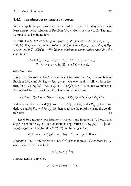
1.4 — General domains 57
1.4.2 An abstract symmetry theorem
We now apply the previous uniqueness result to deduce partial symmetries ofleast energy nodal solution of Problem (Pp) when p is close to 2. The nextLemma is the key ingredient.
Lemma 1.4.3. Let M > 0, p be given by Proposition 1.4.2 and e2 ∈ E2 \B(0, 1
M ). If up is a solution of Problem (Pp) such that PE2up = e2 and up ∈ BM ,p < p, and if T : H1
0 (Ω)→ H10 (Ω) is a continuous isomorphism satisfying the
conditions:
(i) T (E2) = E2; (ii) T (E⊥2 ) = E⊥2 ; (iii) Te2 = e2;(iv) for every u ∈ H1
0 (Ω), Ep(Tu) = Ep(u);
then Tup = up.
Proof. By Proposition 1.4.2, it is sufficient to prove that Tup is a solution ofProblem (Pp) and PE2 Tup = PE2 up = e2. On one hand, it follows from (iv)that, for all v ∈ H1
0 (Ω), 〈dEp(Tup),v〉= 〈dEp(up),T−1v〉, so that we infer thatTup is a solution of Problem (Pp). On the other hand, since
PE2Tup +PE⊥2Tup = Tup = T PE2up +T PE⊥2
up = PE2Tup +PE⊥2Tup,
and the conditions (i) and (ii) ensure that T PE2up ∈ E2 and T PE⊥2up ∈ E⊥2 , we
deduce that PE2Tup = T PE2up. We then conclude the proof by using the condi-tion (iii).
Let G be a group whose identity is written 1 and inverse (.)−1. Recall thata group action on H1
0 (Ω) is a continuous application G×H10 (Ω)→ H1
0 (Ω) :(g,u) 7→ gu such that, for all u ∈ H1
0 (Ω) and for all g,h ∈ G,
(i) 1u = u, (ii) (gh)u = g(hu), (iii) u 7→ gu is linear.
Example 1.4.4. To any subgroup G of O(N) such that g(Ω) = Ω for every g∈G,one can associate the action
gu(x) := u(g−1x).
Another action is given by
gu(x) := (detg)u(g−1x).
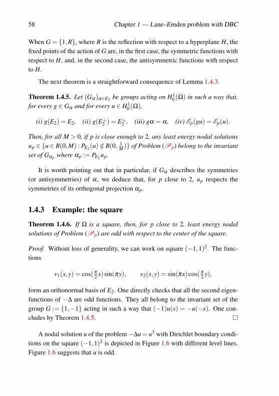
58 Chapter 1 — Lane–Emden problem with DBC
When G = 1,R, where R is the reflection with respect to a hyperplane H, thefixed points of the action of G are, in the first case, the symmetric functions withrespect to H, and, in the second case, the antisymmetric functions with respectto H.
The next theorem is a straightforward consequence of Lemma 1.4.3.
Theorem 1.4.5. Let (Gα)α∈E2 be groups acting on H10 (Ω) in such a way that,
for every g ∈ Gα and for every u ∈ H10 (Ω),
(i) g(E2) = E2, (ii) g(E⊥2 ) = E⊥2 , (iii) gα = α , (iv) Ep(gu) = Ep(u).
Then, for all M > 0, if p is close enough to 2, any least energy nodal solutionsup ∈ u ∈ B(0,M) : PE2(u) /∈ B(0, 1
M ) of Problem (Pp) belong to the invariantset of Gαp where αp := PE2up.
It is worth pointing out that in particular, if Gα describes the symmetries(or antisymmetries) of α , we deduce that, for p close to 2, up respects thesymmetries of its orthogonal projection αp.
1.4.3 Example: the square
Theorem 1.4.6. If Ω is a square, then, for p close to 2, least energy nodalsolutions of Problem (Pp) are odd with respect to the center of the square.
Proof. Without loss of generality, we can work on square (−1,1)2. The func-tions
v1(x,y) = cos(π
2 x)sin(πy), v2(x,y) = sin(πx)cos(π
2 y),
form an orthonormal basis of E2. One directly checks that all the second eigen-functions of −∆ are odd functions. They all belong to the invariant set of thegroup G := 1,−1 acting in such a way that (−1)u(x) = −u(−x). One con-cludes by Theorem 1.4.5.
A nodal solution u of the problem−∆u = u3 with Dirichlet boundary condi-tions on the square (−1,1)2 is depicted in Figure 1.6 with different level lines.Figure 1.6 suggests that u is odd.
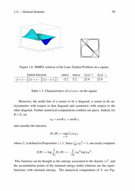
1.4 — General domains 59
−4
−3
−2
−1
0
1
2
3
4
Z
0.00.5
1.01.5
2.02.5
3.03.5
Y
0.00.5
1.01.5
2.02.5
3.03.5X
Figure 1.6: MMPA solution of the Lane–Emden Problem on a square.
Initial function minu maxu E4(u+) E4(u−)(x+ y− 2
5 )(x+ y− 85 )(x− y± 3
5 ) −5.2 5.2 23.9 23.9
Table 1.3: Characteristics of a l.e.n.s. on the square.
Moreover, the nodal line of u seems to be a diagonal, u seems to be an-tisymmetric with respect to that diagonal and symmetric with respect to theother diagonal. Further numerical computations confirm our guess. Indeed, forθ ∈ R, set
vθ = cosθ v1 + sinθ v2
and consider the function
H∗(θ) := supt>0
E∗(tvθ ),
where E∗ is defined in Proposition 1.1.3. Since∫
Ω|vθ |2 = 1, one easily computes
S(θ) := log2λ2
H∗(θ) =−∫
Ω
|vθ |2 log|vθ |2.
This function can be thought as the entropy associated to the density |v|2, andthe accumulation points of the minimal energy nodal solutions are the eigen-functions with minimal entropy. The numerical computation of S, see Fig-
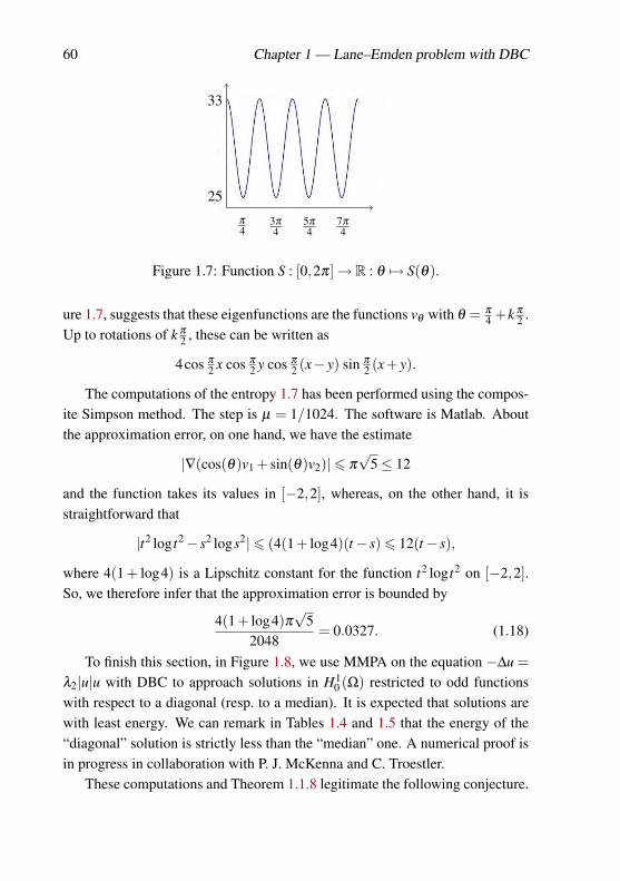
60 Chapter 1 — Lane–Emden problem with DBC
π
43π
45π
47π
4
33
25
Figure 1.7: Function S : [0,2π]→ R : θ 7→ S(θ).
ure 1.7, suggests that these eigenfunctions are the functions vθ with θ = π
4 +k π
2 .Up to rotations of k π
2 , these can be written as
4cos π
2 x cos π
2 y cos π
2 (x− y) sin π
2 (x+ y).
The computations of the entropy 1.7 has been performed using the compos-ite Simpson method. The step is µ = 1/1024. The software is Matlab. Aboutthe approximation error, on one hand, we have the estimate
|∇(cos(θ)v1 + sin(θ)v2)|6 π√
5≤ 12
and the function takes its values in [−2,2], whereas, on the other hand, it isstraightforward that
|t2 log t2− s2 logs2|6 (4(1+ log4)(t− s)6 12(t− s),
where 4(1 + log4) is a Lipschitz constant for the function t2 log t2 on [−2,2].So, we therefore infer that the approximation error is bounded by
4(1+ log4)π√
52048
= 0.0327. (1.18)
To finish this section, in Figure 1.8, we use MMPA on the equation −∆u =λ2|u|u with DBC to approach solutions in H1
0 (Ω) restricted to odd functionswith respect to a diagonal (resp. to a median). It is expected that solutions arewith least energy. We can remark in Tables 1.4 and 1.5 that the energy of the“diagonal” solution is strictly less than the “median” one. A numerical proof isin progress in collaboration with P. J. McKenna and C. Troestler.
These computations and Theorem 1.1.8 legitimate the following conjecture.
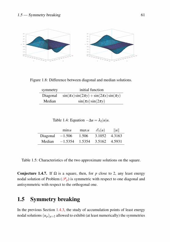
1.5 — Symmetry breaking 61
−2.0
−1.5
−1.0
−0.5
0.0
0.5
1.0
1.5
2.0
Z
0.00.10.20.30.40.50.60.70.80.91.0 X
0.0 0.1 0.2 0.3 0.4 0.5 0.6 0.7 0.8 0.9 1.0Y
−2.0
−1.5
−1.0
−0.5
0.0
0.5
1.0
1.5
2.0
Z
0.00.10.20.30.40.50.60.70.80.91.0 X
0.0 0.1 0.2 0.3 0.4 0.5 0.6 0.7 0.8 0.9 1.0Y
Figure 1.8: Difference between diagonal and median solutions.
symmetry initial functionDiagonal sin(πx)sin(2πy)+ sin(2πx)sin(πy)Median sin(πx)sin(2πy)
Table 1.4: Equation −∆u = λ2|u|u.
minu maxu E3(u) ‖u‖Diagonal −1.506 1.506 3.1052 4.3163Median −1.5354 1.5354 3.5162 4.5931
Table 1.5: Characteristics of the two approximate solutions on the square.
Conjecture 1.4.7. If Ω is a square, then, for p close to 2, any least energynodal solution of Problem (Pp) is symmetric with respect to one diagonal andantisymmetric with respect to the orthogonal one.
1.5 Symmetry breaking
In the previous Section 1.4.3, the study of accumulation points of least energynodal solutions (up)p>2 allowed to exhibit (at least numerically) the symmetries
62 Chapter 1 — Lane–Emden problem with DBC
of least energy nodal solutions for p close to 2 on the square. In the same way,under the assumption that the minima of the entropy function S are not given by“median” functions (as suggested on Figure 1.7), this analysis can also be usedto obtain some symmetry breaking for larger p. We begin by studying smallperturbations of the Laplacian.
1.5.1 Perturbation of the Laplacian operator
The previous results, related to general domains, can be extended to Prob-lem (Pp)
−div(Ap∇u) = λ2|u|p−2u, in Ω,
u = 0, on ∂Ω,(Pp)
with Ap ∈ C (Ω,MN×N), where MN×N is the set of symmetric N×N matrices,is such that A2 = id and p 7→ Ap is uniformly differentiable at p = 2 (i.e. thereexists a matrix A′2 ∈MN×N verifying∥∥∥Ap−A2−A′2(p−2)
p−2
∥∥∥∞
→ 0, as p→ 2).
We are interested in critical points of the functional
Ep : H10 (Ω)→ R : u 7→ 1
2
∫Ω
(Ap∇u) ·∇u− λ2
p
∫Ω
|u|p.
Theorem 1.5.1. Let (up)p>2 be least energy nodal solutions of Problem (Pp).If upn u∗ in H1
0 (Ω) for some sequence pn→ 2, then upn → u∗ 6= 0 in H10 (Ω),
u∗ satisfies −∆u∗ = λ2u∗, in Ω,
u∗ = 0, on ∂Ω,
and
E∗(u∗) = infE∗(u) : u ∈ E2 \0,〈dE∗(u),u〉= 0,
where
E∗ : E2→ R : u 7→∫
Ω
(A′2∇u) ·∇u+λ2
2(u2−u2 logu2).
1.5 — Symmetry breaking 63
Sketch of the proof. All the arguments developed in Section 1.1 hold for (Pp),up to some small differences. Indeed, the equations (1.6) and (1.7) becomerespectively
−∆w−λ2w = div(A′2∇u∗)+λ2u∗ log |u∗|,PE2w = 0,
and∫Ω
|∇v±p |2 = λ2
∫Ω
(vp +(p−2)u∗ log |u∗|)v±p − (p−2)∫
Ω
(A′2∇u∗) ·∇v±p
= λ2
∫Ω
|v±p |p− (p−2)∫
Ω
(A′2∇u∗) ·∇v±p +o(p−2).
The computation of t±p gives
(t±p )p−2 =(Ap∇v+
p ) ·∇v+p
λ2‖v±p ‖pp
=‖∇v±p ‖2
2 +(p−2)∫
Ω
(Ap− idp−2
∇vp
)·∇v±p
λ2‖v±p ‖pp
,
and the proof that t±p → 1 follows from the fact that
(p−2)∫
Ω
(Ap−idp−2 ∇vp
)·∇v±p − (p−2)
∫Ω(A′2∇u∗) ·∇v±p
= (p−2)∫
Ω
((Ap−idp−2 −A′2
)∇vp
)·∇v±p +(p−2)2 ∫
Ω(A′2∇w) ·∇v±p
= o(p−2),
giving then the same conclusion as for Problem (Pp).In a similar fashion, all the other results extend to the present framework.
Observe that it is enough to have the differentiability along the sequences.Going to the abstract symmetry results, Proposition 1.4.2 about the unique-
ness of the solution with a given projection on E2 extends immediately to Prob-lem (Pp).
Proposition 1.5.2. For every M > 0, there exists p > 2 such that, for everyp ∈ (2, p) , if up,vp ∈ u ∈ B(0,M) : PE2 /∈ B(0, 1
M ) solve the boundary valueproblem
−div(Ap∇u) = λ2|u|p−2u, in Ω,
u = 0, on ∂Ω,
then PE2up = PE2vp implies up = vp.
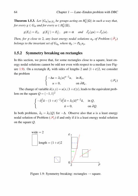
64 Chapter 1 — Lane–Emden problem with DBC
Theorem 1.5.3. Let (Gα)α∈E2 be groups acting on H10 (Ω) in such a way that,
for every g ∈ Gα and for every u ∈ H10 (Ω),
g(E2) = E2, g(E⊥2 ) = E⊥2 , gα = α and Ep(gu) = Ep(u).
Then, for p close to 2, any least energy nodal solutions up of Problem (Pp)belongs to the invariant set of Gαp where αp := PE2up.
1.5.2 Symmetry breaking on rectangles
In this section, we prove that, for some rectangles close to a square, least en-ergy nodal solutions cannot be odd nor even with respect to a median (see Fig-ure 1.9). On a rectangle Rε with sides of lengths 2 and (1 + ε)2, we considerthe problem
−∆u = λ2|u|p−2u, in Rε ,
u = 0, on ∂Rε .(Pε )
The change of variable u(x,y) = u(x,(1+ε)y), leads to the equivalent prob-lem on the square Q = (−1,1)2
−∂2x u− (1+ ε)−2
∂2y u = λ2|u|p−2u, in Q,
u = 0, on ∂Q.
In both problems, λ2 = λ2(Q) for −∆. Observe also that u is a least energynodal solution of Problem (Pε ) if and only if u is a least energy nodal solutionon the square Q.
20 p
εwide = 2
length = (1+ ε)2
Figure 1.9: Symmetry breaking: rectangles→ square.
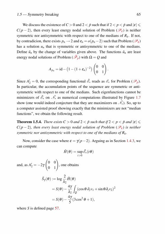
1.5 — Symmetry breaking 65
We discuss the existence of C > 0 and 2 < p such that if 2 < p < p and |ε|6C(p− 2), then every least energy nodal solution of Problem (Pε ) is neithersymmetric nor antisymmetric with respect to one of the medians of Rε . If not,by contradicion, there exists pn→ 2 and εn = o(pn−2) such that Problem (Pε )has a solution un that is symmetric or antisymmetric to one of the medians.Define un by the change of variables given above. The functions un are leastenergy nodal solutions of Problem (Pp) with Ω = Q and
Apn = id−(1− (1+ εn)−2)(0 0
0 1
).
Since A′2 = 0, the corresponding functional E∗ reads as E∗ for Problem (Pp).In particular, the accumulation points of the sequence are symmetric or anti-symmetric with respect to one of the medians. Such eigenfunctions cannot beminimizers of E∗ on ˜N∗ as numerical computations illustrated by Figure 1.7show (one would indeed conjecture that they are maximizers on ˜N∗). So, up toa computer assisted proof showing exactly that the minimizers are not “medianfunctions”, we obtain the following result.
Theorem 1.5.4. There exists C > 0 and 2 < p such that if 2 < p < p and |ε|6C(p− 2), then every least energy nodal solution of Problem (Pε ) is neithersymmetric nor antisymmetric with respect to one of the medians of Rε .
Now, consider the case where ε = γ(p−2). Arguing as in Section 1.4.3, wecan compute
H(θ) = supt>0
E∗(tθ)
and, as A′2 =−2γ
(0 00 1
), one obtains
Sγ(θ) := log2λ2
H(θ)
= S(θ)− 4γ
λ2
∫Q(cosθ ∂yv1 + sinθ∂yv2)2
= S(θ)− 4γ
5(3cos2
θ +1),
where S is defined page 57.
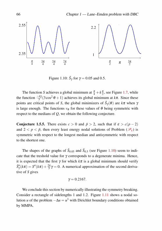
66 Chapter 1 — Lane–Emden problem with DBC
π
43π
45π
47π
4
2.55
2.35
π
2 π 3π
2
2.2
1
Figure 1.10: Sγ for γ = 0.05 and 0.5.
The function S achieves a global minimum at π
4 + k π
2 , see Figure 1.7, whilethe function −4γ
5 (3cos2 θ + 1) achieves its global minimum at kπ . Since thesepoints are critical points of S, the global minimizers of Sγ(θ) are kπ when γ
is large enough. The functions vθ for these values of θ being symmetric withrespect to the medians of Q, we obtain the following conjecture.
Conjecture 1.5.5. There exists c > 0 and p > 2, such that if ε > c(p− 2)and 2 < p < p, then every least energy nodal solutions of Problem (Pε ) issymmetric with respect to the longest median and antisymmetric with respectto the shortest one.
The shapes of the graphs of S0.05 and S0.5 (see Figure 1.10) seem to indi-cate that the treshold value for γ corresponds to a degenerate minima. Hence,it is expected that the first γ for which kπ is a global minimum should verifyS′′γ (kπ) = S′′(kπ)+ 24
5 γ = 0. A numerical approximation of the second deriva-tive of S gives
γ = 0.2167.
We conclude this section by numerically illustrating the symmetry breaking.Consider a rectangle of sidelengths 1 and 1.2. Figure 1.11 shows a nodal so-lution u of the problem −∆u = u3 with Dirichlet boundary conditions obtainedby MMPA.
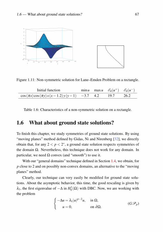
1.6 — What about ground state solutions? 67
−4
−3
−2
−1
0
1
2
3
4
5
Z
0.00.20.40.60.81.01.2
X
0.00.5
1.0Y
Figure 1.11: Non-symmetric solution for Lane–Emden Problem on a rectangle.
Initial function minu maxu E4(u+) E4(u−)cos(πx)cos(πy)x(x−1.2)y(y−1) −3.7 4.2 19.7 26.2
Table 1.6: Characteristics of a non-symmetric solution on a rectangle.
1.6 What about ground state solutions?
To finish this chapter, we study symmetries of ground state solutions. By using“moving planes” method defined by Gidas, Ni and Nirenberg [32], we directlyobtain that, for any 2 < p < 2∗, a ground state solution respects symmetries ofthe domain Ω. Nevertheless, this technique does not work for any domain. Inparticular, we need Ω convex (and “smooth”) to use it.
With our “general domains” technique defined in Section 1.4, we obtain, forp close to 2 and on possibly non-convex domains, an alternative to the “movingplanes” method.
Clearly, our technique can very easily be modified for ground state solu-tions. About the asymptotic behavior, this time, the good rescaling is given byλ1, the first eigenvalue of −∆ in H1
0 (Ω) with DBC. Now, we are working withthe problem
−∆u = λ1|u|p−2u, in Ω,
u = 0, on ∂Ω.(GPp)
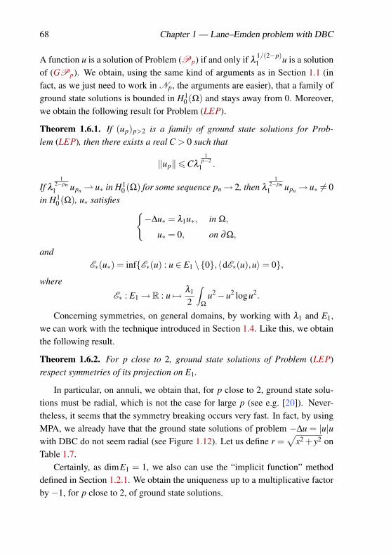
68 Chapter 1 — Lane–Emden problem with DBC
A function u is a solution of Problem (Pp) if and only if λ1/(2−p)1 u is a solution
of (GPp). We obtain, using the same kind of arguments as in Section 1.1 (infact, as we just need to work in Np, the arguments are easier), that a family ofground state solutions is bounded in H1
0 (Ω) and stays away from 0. Moreover,we obtain the following result for Problem (LEP).
Theorem 1.6.1. If (up)p>2 is a family of ground state solutions for Prob-lem (LEP), then there exists a real C > 0 such that
‖up‖6Cλ
1p−2
1 .
If λ
12−pn
1 upn u∗ in H10 (Ω) for some sequence pn→ 2, then λ
12−pn
1 upn → u∗ 6= 0in H1
0 (Ω), u∗ satisfies −∆u∗ = λ1u∗, in Ω,
u∗ = 0, on ∂Ω,
andE∗(u∗) = infE∗(u) : u ∈ E1 \0,〈dE∗(u),u〉= 0,
where
E∗ : E1→ R : u 7→ λ1
2
∫Ω
u2−u2 logu2.
Concerning symmetries, on general domains, by working with λ1 and E1,we can work with the technique introduced in Section 1.4. Like this, we obtainthe following result.
Theorem 1.6.2. For p close to 2, ground state solutions of Problem (LEP)respect symmetries of its projection on E1.
In particular, on annuli, we obtain that, for p close to 2, ground state solu-tions must be radial, which is not the case for large p (see e.g. [20]). Never-theless, it seems that the symmetry breaking occurs very fast. In fact, by usingMPA, we already have that the ground state solutions of problem −∆u = |u|uwith DBC do not seem radial (see Figure 1.12). Let us define r =
√x2 + y2 on
Table 1.7.Certainly, as dimE1 = 1, we also can use the “implicit function” method
defined in Section 1.2.1. We obtain the uniqueness up to a multiplicative factorby −1, for p close to 2, of ground state solutions.
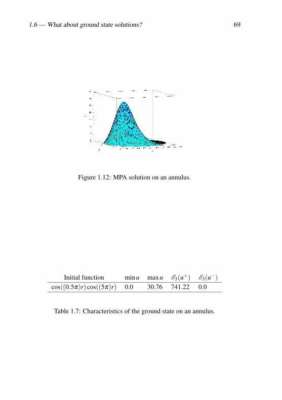
1.6 — What about ground state solutions? 69
Figure 1.12: MPA solution on an annulus.
Initial function minu maxu E3(u+) E3(u−)cos((0.5π)r)cos((5π)r) 0.0 30.76 741.22 0.0
Table 1.7: Characteristics of the ground state on an annulus.
70 Chapter 1 — Lane–Emden problem with DBC
Chapter 2
Nodal line structure of leastenergy nodal solutions
In this chapter, we are interested in the nodal line structure of least energynodal solutions for the Lane–Emden Problem with DBC (Pp)
−∆u = λ2|u|p−2u, in Ω,
u = 0, on ∂Ω,
where Ω⊆ R2 is an open bounded connected domain and p > 2. In Chapter 1,we studied some symmetries of solutions on rectangles, balls, annuli, squares,...In particular, for these domains, we obtained that the nodal line of least energynodal solutions intersects ∂Ω, at least for p close to 2. We would like to know,for which domains Ω not necessarily symmetric and 2 < p < 2∗, the nodalline of a least energy nodal solution intersects ∂Ω. In Theorem 1.1.8, it isproved that a family of least energy nodal solutions (up)p>2 of Problem (Pp)is bounded in H1
0 (Ω) and stays away from the zero function. Moreover, weakaccumulation points for the H1
0 -norm are in fact strong accumulation pointsbelonging to E2. A H1
0 -convergence is clearly not enough to control the levelcurves and to solve the problem. Here, we establish that (up)p>2 converges, in asuitable sense, to some u∗ ∈E2 in a such a manner that the zero set of up is closeto the zero set of u∗. We obtain that the nodal line intersects the boundary when
71
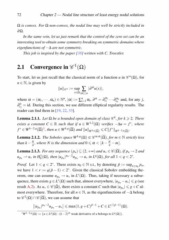
72 Chapter 2 — Nodal line structure of least energy nodal solutions
Ω is convex. For Ω non-convex, the nodal line may well be strictly included in∂Ω.
In the same vein, let us just remark that the control of the zero set can be aninteresting tool to obtain some symmetry breaking on symmetric domains whereeigenfunctions of −∆ are not symmetric.
This job is inspired by the paper [38] written with C. Troestler.
2.1 Convergence in C 1(Ω)
To start, let us just recall that the classical norm of a function u in C n(Ω), forn ∈ N, is given by
‖u‖C n := supx∈Ω
∑|α|≤n|∂ α u(x)|,
where α = (α1, · · · ,αn) ∈ Nn, |α| := ∑ni=1 αi, ∂ α = ∂
α1x1 · · ·∂ αn
xn and, for any j,∂ 0
x j= id. During this section, we use different elliptical regularity results. The
reader can find them in [19, 22, 33].
Lemma 2.1.1. Let Ω be a bounded open domain of class C k, for k > 2. Thereexists a constant C ∈ R such that if u ∈W 1,2(Ω) verifies −∆u = f ∗, wheref ∗ ∈W k−2,q(Ω)1, then u ∈W k,q(Ω) and ‖u‖W k,q(Ω) 6C‖ f ∗‖W k−2,q(Ω).
Lemma 2.1.2. The Sobolev space W k,q(Ω)b C m,α(Ω), for m ∈ N strictly lessthan k− N
q , where N is the dimension and 06 α < bk− Nq −mc.
Lemma 2.1.3. For any sequence (pn)⊆ (2,+∞) and u∗ ∈C (Ω), if pn→ 2 andupn u∗ in H1
0 (Ω), then |upn |pn−2upn → u∗ in Lq(Ω), for all 1 < q < 2∗.
Proof. Let 1 < q < 2∗. There exists n0 ∈ N s.t., by denoting p := supn≥n0pn,
we have 1 < r := q(p− 1) < 2∗. Given the classical Sobolev embedding the-orem, one can assume upn → u∗ in Lr(Ω). Thus, taking if necessary a subse-quence, there exists g∈ Lr(Ω) such that, almost everywhere, |upn−u∗|6 g (seeresult A.2). As u∗ ∈ C (Ω), there exists a constant C such that |upn |6 g+C al-most everywhere. Therefore, for all n ∈ N, as the eigenfunctions of −∆ belongto C 2(Ω)∩C (Ω), we can assume that∣∣|upn |pn−2upn −u∗
∣∣6max(1,g+C)p−1 +C ∈ Lr/(p−1)(Ω).
1W k−2,q(Ω) := u ∈ Lq(Ω) : (k−2)th weak derivative of u belongs to Lq(Ω).
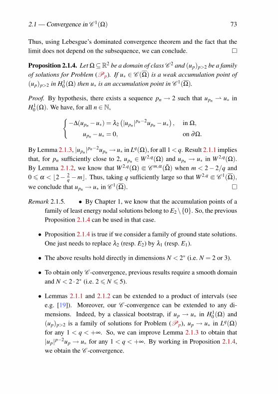
2.1 — Convergence in C 1(Ω) 73
Thus, using Lebesgue’s dominated convergence theorem and the fact that thelimit does not depend on the subsequence, we can conclude.
Proposition 2.1.4. Let Ω⊆R2 be a domain of class C 2 and (up)p>2 be a familyof solutions for Problem (Pp). If u∗ ∈ C (Ω) is a weak accumulation point of(up)p>2 in H1
0 (Ω) then u∗ is an accumulation point in C 1(Ω).
Proof. By hypothesis, there exists a sequence pn → 2 such that upn u∗ inH1
0 (Ω). We have, for all n ∈ N,−∆(upn −u∗) = λ2
(|upn |pn−2upn −u∗
), in Ω,
upn −u∗ = 0, on ∂Ω.
By Lemma 2.1.3, |upn |pn−2upn→ u∗ in Lq(Ω), for all 1 < q. Result 2.1.1 impliesthat, for pn sufficiently close to 2, upn ∈W 2,q(Ω) and upn → u∗ in W 2,q(Ω).By Lemma 2.1.2, we know that W 2,q(Ω) b C m,α(Ω) when m < 2− 2/q and0 6 α < b2− 2
q −mc. Thus, taking q sufficiently large so that W 2,q b C 1(Ω),we conclude that upn → u∗ in C 1(Ω).
Remark 2.1.5. • By Chapter 1, we know that the accumulation points of afamily of least energy nodal solutions belong to E2\0. So, the previousProposition 2.1.4 can be used in that case.
• Proposition 2.1.4 is true if we consider a family of ground state solutions.One just needs to replace λ2 (resp. E2) by λ1 (resp. E1).
• The above results hold directly in dimensions N < 2∗ (i.e. N = 2 or 3).
• To obtain only C -convergence, previous results require a smooth domainand N < 2 ·2∗ (i.e. 26 N 6 5).
• Lemmas 2.1.1 and 2.1.2 can be extended to a product of intervals (seee.g. [19]). Moreover, our C -convergence can be extended to any di-mensions. Indeed, by a classical bootstrap, if up → u∗ in H1
0 (Ω) and(up)p>2 is a family of solutions for Problem (Pp), up → u∗ in Lq(Ω)for any 1 < q < +∞. So, we can improve Lemma 2.1.3 to obtain that|up|p−2up → u∗ for any 1 < q < +∞. By working in Proposition 2.1.4,we obtain the C -convergence.
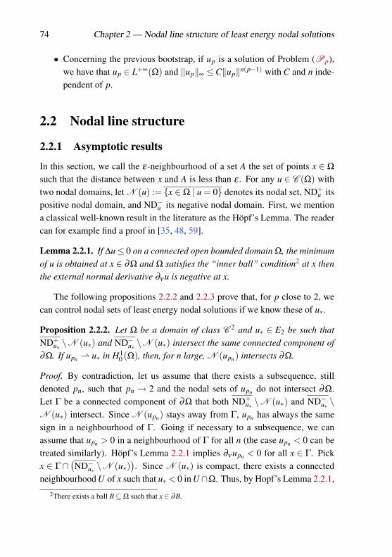
74 Chapter 2 — Nodal line structure of least energy nodal solutions
• Concerning the previous bootstrap, if up is a solution of Problem (Pp),we have that up ∈ L+∞(Ω) and ‖up‖∞ ≤C‖up‖n(p−1) with C and n inde-pendent of p.
2.2 Nodal line structure
2.2.1 Asymptotic results
In this section, we call the ε-neighbourhood of a set A the set of points x ∈ Ω
such that the distance between x and A is less than ε . For any u ∈ C (Ω) withtwo nodal domains, let N (u) := x ∈Ω | u = 0 denotes its nodal set, ND+
u itspositive nodal domain, and ND−u its negative nodal domain. First, we mentiona classical well-known result in the literature as the Höpf’s Lemma. The readercan for example find a proof in [35, 48, 59].
Lemma 2.2.1. If ∆u≤ 0 on a connected open bounded domain Ω, the minimumof u is obtained at x ∈ ∂Ω and Ω satisfies the “inner ball” condition2 at x thenthe external normal derivative ∂ν u is negative at x.
The following propositions 2.2.2 and 2.2.3 prove that, for p close to 2, wecan control nodal sets of least energy nodal solutions if we know these of u∗.
Proposition 2.2.2. Let Ω be a domain of class C 2 and u∗ ∈ E2 be such thatND+
u∗ \N (u∗) and ND−u∗ \N (u∗) intersect the same connected component of∂Ω. If upn u∗ in H1
0 (Ω), then, for n large, N (upn) intersects ∂Ω.
Proof. By contradiction, let us assume that there exists a subsequence, stilldenoted pn, such that pn → 2 and the nodal sets of upn do not intersect ∂Ω.Let Γ be a connected component of ∂Ω that both ND+
u∗ \N (u∗) and ND−u∗ \N (u∗) intersect. Since N (upn) stays away from Γ, upn has always the samesign in a neighbourhood of Γ. Going if necessary to a subsequence, we canassume that upn > 0 in a neighbourhood of Γ for all n (the case upn < 0 can betreated similarly). Höpf’s Lemma 2.2.1 implies ∂ν upn < 0 for all x ∈ Γ. Pickx ∈ Γ∩
(ND−u∗ \N (u∗)
). Since N (u∗) is compact, there exists a connected
neighbourhood U of x such that u∗ < 0 in U∩Ω. Thus, by Hopf’s Lemma 2.2.1,
2There exists a ball B⊆Ω such that x ∈ ∂B.
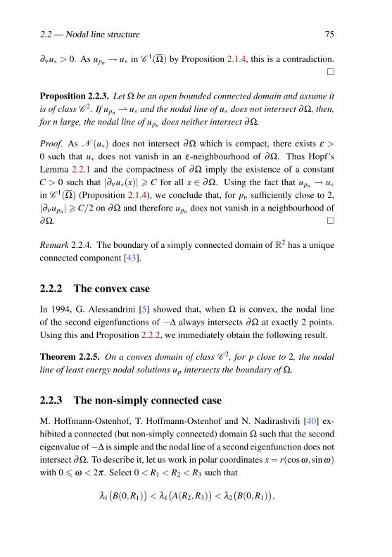
2.2 — Nodal line structure 75
∂ν u∗ > 0. As upn → u∗ in C 1(Ω) by Proposition 2.1.4, this is a contradiction.
Proposition 2.2.3. Let Ω be an open bounded connected domain and assume itis of class C 2. If upn u∗ and the nodal line of u∗ does not intersect ∂Ω, then,for n large, the nodal line of upn does neither intersect ∂Ω.
Proof. As N (u∗) does not intersect ∂Ω which is compact, there exists ε >
0 such that u∗ does not vanish in an ε-neighbourhood of ∂Ω. Thus Hopf’sLemma 2.2.1 and the compactness of ∂Ω imply the existence of a constantC > 0 such that |∂ν u∗(x)| > C for all x ∈ ∂Ω. Using the fact that upn → u∗in C 1(Ω) (Proposition 2.1.4), we conclude that, for pn sufficiently close to 2,|∂ν upn |>C/2 on ∂Ω and therefore upn does not vanish in a neighbourhood of∂Ω.
Remark 2.2.4. The boundary of a simply connected domain of R2 has a uniqueconnected component [43].
2.2.2 The convex case
In 1994, G. Alessandrini [5] showed that, when Ω is convex, the nodal lineof the second eigenfunctions of −∆ always intersects ∂Ω at exactly 2 points.Using this and Proposition 2.2.2, we immediately obtain the following result.
Theorem 2.2.5. On a convex domain of class C 2, for p close to 2, the nodalline of least energy nodal solutions up intersects the boundary of Ω.
2.2.3 The non-simply connected case
M. Hoffmann-Ostenhof, T. Hoffmann-Ostenhof and N. Nadirashvili [40] ex-hibited a connected (but non-simply connected) domain Ω such that the secondeigenvalue of−∆ is simple and the nodal line of a second eigenfunction does notintersect ∂Ω. To describe it, let us work in polar coordinates x = r(cosω,sinω)with 06 ω < 2π . Select 0 < R1 < R2 < R3 such that
λ1(B(0,R1)
)< λ1
(A(R2,R3)
)< λ2
(B(0,R1)
),
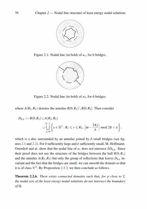
76 Chapter 2 — Nodal line structure of least energy nodal solutions
Figure 2.1: Nodal line (in bold) of u∗, for 6 bridges.
Figure 2.2: Nodal line (in bold) of u3, for 6 bridges.
where A(R2,R3) denotes the annulus B(0,R3)\B[0,R2]. Then consider
Db,ε := B(0,R1)∪A(R2,R3)
∪b−1⋃j=0
x ∈ R2 : R1 6 r 6 R2,
∣∣∣ω− 2π jb
∣∣∣ mod 2π < ε
,
which is a disc surrounded by an annulus joined by b small bridges (see fig-ures 2.1 and 2.2). For b sufficiently large and ε sufficiently small, M. Hoffmann-Ostenhof and al. show that the nodal line of u∗ does not intersect ∂Db,ε . Sincetheir proof does not use the structure of the bridges between the ball B(0,R1)and the annulus A(R2,R3) but only the group of reflections that leaves Db,ε in-variant and the fact that the bridges are small, we can smooth the domain so thatit is of class C 2. By Proposition 2.2.3, we then conclude as follows.
Theorem 2.2.6. There exists connected domains such that, for p close to 2,the nodal sets of the least energy nodal solutions do not intersect the boundaryof Ω.
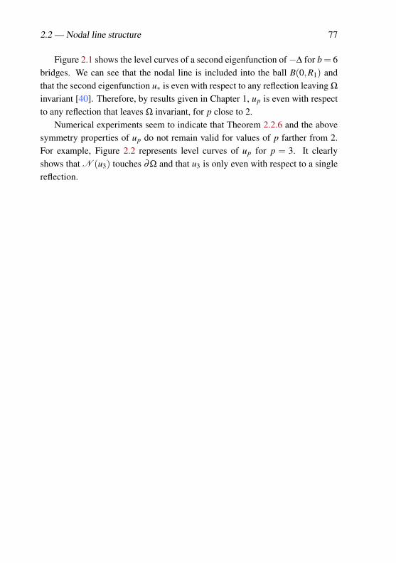
2.2 — Nodal line structure 77
Figure 2.1 shows the level curves of a second eigenfunction of−∆ for b = 6bridges. We can see that the nodal line is included into the ball B(0,R1) andthat the second eigenfunction u∗ is even with respect to any reflection leaving Ω
invariant [40]. Therefore, by results given in Chapter 1, up is even with respectto any reflection that leaves Ω invariant, for p close to 2.
Numerical experiments seem to indicate that Theorem 2.2.6 and the abovesymmetry properties of up do not remain valid for values of p farther from 2.For example, Figure 2.2 represents level curves of up for p = 3. It clearlyshows that N (u3) touches ∂Ω and that u3 is only even with respect to a singlereflection.
78 Chapter 2 — Nodal line structure of least energy nodal solutions
Chapter 3
Schrödinger and q-LaplacianLane–Emden problem
From Chapter 3 to Chapter 5, we generalize results presented in Chapter 1.We would like to know whether asymptotic and symmetry results are workingfor more general problems. Concerning symmetry (or non-symmetry) results,we will essentially focus on the “general method” studied in Section 1.4 inorder to study general domains and obtain some symmetry breaking. In thischapter, we work with some perturbations of the linear part ∆ of Problem (Pp).Let us just remark that, in Chapter 1 (see Section 1.5), we already proved thatasymptotic and symmetry results are valid for Problem (Pp)
−div(Ap∇u) = λ |u|p−2u, in Ω,
u = 0, on ∂Ω,
with Ap ∈ C (Ω,MN×N), where MN×N is the set of symmetric N×N matrices,such that A2 = id and p 7→ Ap is uniformly differentiable at p = 2.
In Section 3.1, we are studying the superlinear elliptic boundary value Prob-lem (SPp) of Schrödinger type
−∆u+Vu = λ |u|p−2u, in Ω,
u = 0, on ∂Ω,(SPp)
79
80 Chapter 3 — Schrödinger and q-Laplacian problem
where λ > 0. We study Problem (SPp) for a continuous potential V : Ω→ Rsuch that −∆ +V is compact and positive definite1. Under these assumptions,we work in H1
0 (Ω) with the scalar product (u|v) =∫
Ω∇u ·∇v +V (x)uv and
associated norm
‖u‖2 =∫
Ω
|∇u|2 +V (x)u2. (3.1)
The energy functional Ep is given by
H10 (Ω)→ R : u 7→ 1
2
∫Ω
|∇u|2 +V (x)u2− λ
p
∫Ω
|u|p,
which does not change anything about the existence of ground state solutions(resp. l.e.n.s.). They can again be defined as minima of the energy functional Ep
on the Nehari manifold
Np :=
u ∈ H10 (Ω)\0
∣∣ ∫Ω
|∇u|2 +V (x)u2 = λ
∫Ω
|u|p
(resp. Mp := u : u± ∈Np). Let us just remark that, if −∆+V is not positivedefinite, the zero function may not be a local minimum of Ep anymore. Thereexist directions without functions belonging to Np. So, the approach defined inChapter 1 does not work (see Proposition 1.1.1 or Chapter 6 for more infor-mation). Under our assumptions, we prove that our asymptotic behavior andsymmetry results are still working. We denote by λi (resp. Ei) the distinct eigen-values (resp. eigenspaces) of −∆+V with DBC. As in Chapter 1, we show thata family of ground state solutions (resp. l.e.n.s.) converges up to a subsequenceto a non-zero function if and only if λ = λ1 (resp. λ2). Depending on symme-tries of eigenfunctions for −∆ +V , we obtain the symmetry results. Of course,results given in Chapter 2 related to the C -convergence can also be used in thatcase.
In Section 3.2, we study what happens for the q-Laplacian Lane–EmdenProblem (QLEP)
−∆qu = λ |u|p−2u, in Ω,
u = 0, on ∂Ω.(QPp)
1The eigenvalues are positive.
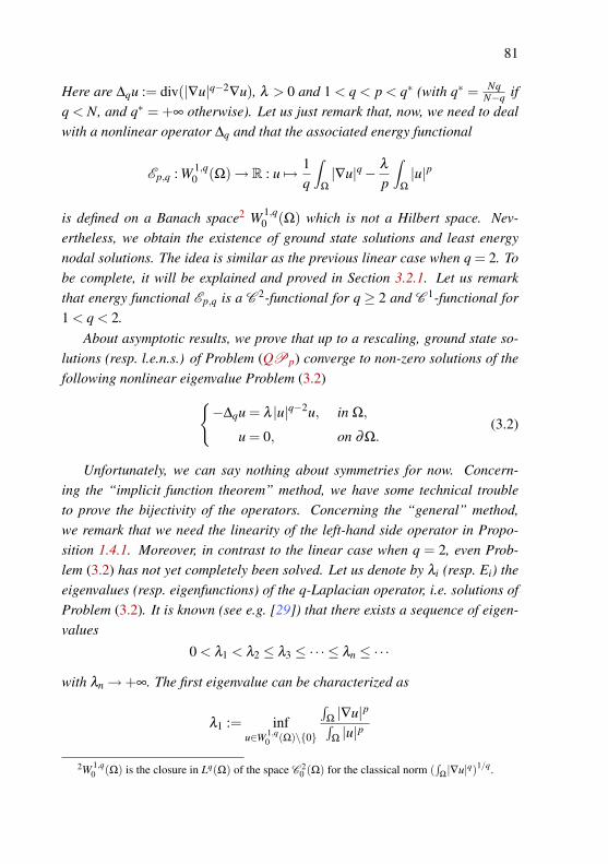
81
Here are ∆qu := div(|∇u|q−2∇u), λ > 0 and 1 < q < p < q∗ (with q∗ = NqN−q if
q < N, and q∗ = +∞ otherwise). Let us just remark that, now, we need to dealwith a nonlinear operator ∆q and that the associated energy functional
Ep,q : W 1,q0 (Ω)→ R : u 7→ 1
q
∫Ω
|∇u|q− λ
p
∫Ω
|u|p
is defined on a Banach space2 W 1,q0 (Ω) which is not a Hilbert space. Nev-
ertheless, we obtain the existence of ground state solutions and least energynodal solutions. The idea is similar as the previous linear case when q = 2. Tobe complete, it will be explained and proved in Section 3.2.1. Let us remarkthat energy functional Ep,q is a C 2-functional for q ≥ 2 and C 1-functional for1 < q < 2.
About asymptotic results, we prove that up to a rescaling, ground state so-lutions (resp. l.e.n.s.) of Problem (QPp) converge to non-zero solutions of thefollowing nonlinear eigenvalue Problem (3.2)
−∆qu = λ |u|q−2u, in Ω,
u = 0, on ∂Ω.(3.2)
Unfortunately, we can say nothing about symmetries for now. Concern-ing the “implicit function theorem” method, we have some technical troubleto prove the bijectivity of the operators. Concerning the “general” method,we remark that we need the linearity of the left-hand side operator in Propo-sition 1.4.1. Moreover, in contrast to the linear case when q = 2, even Prob-lem (3.2) has not yet completely been solved. Let us denote by λi (resp. Ei) theeigenvalues (resp. eigenfunctions) of the q-Laplacian operator, i.e. solutions ofProblem (3.2). It is known (see e.g. [29]) that there exists a sequence of eigen-values
0 < λ1 < λ2 ≤ λ3 ≤ ·· · ≤ λn ≤ ·· ·
with λn→+∞. The first eigenvalue can be characterized as
λ1 := infu∈W 1,q
0 (Ω)\0
∫Ω|∇u|p∫
Ω|u|p
2W 1,q0 (Ω) is the closure in Lq(Ω) of the space C 2
0 (Ω) for the classical norm (∫
Ω|∇u|q)1/q.
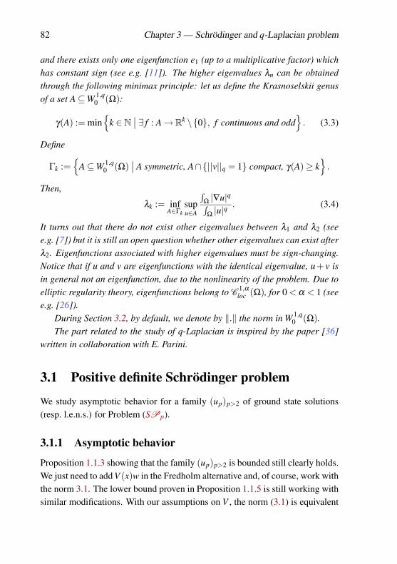
82 Chapter 3 — Schrödinger and q-Laplacian problem
and there exists only one eigenfunction e1 (up to a multiplicative factor) whichhas constant sign (see e.g. [11]). The higher eigenvalues λn can be obtainedthrough the following minimax principle: let us define the Krasnoselskii genusof a set A⊆W 1,q
0 (Ω):
γ(A) := min
k ∈ N∣∣ ∃ f : A→ Rk \0, f continuous and odd
. (3.3)
Define
Γk :=
A⊆W 1,q0 (Ω)
∣∣ A symmetric, A∩||v||q = 1 compact, γ(A)≥ k
.
Then,
λk := infA∈Γk
supu∈A
∫Ω|∇u|q∫
Ω|u|q
. (3.4)
It turns out that there do not exist other eigenvalues between λ1 and λ2 (seee.g. [7]) but it is still an open question whether other eigenvalues can exist afterλ2. Eigenfunctions associated with higher eigenvalues must be sign-changing.Notice that if u and v are eigenfunctions with the identical eigenvalue, u + v isin general not an eigenfunction, due to the nonlinearity of the problem. Due toelliptic regularity theory, eigenfunctions belong to C 1,α
loc (Ω), for 0 < α < 1 (seee.g. [26]).
During Section 3.2, by default, we denote by ‖.‖ the norm in W 1,q0 (Ω).
The part related to the study of q-Laplacian is inspired by the paper [36]written in collaboration with E. Parini.
3.1 Positive definite Schrödinger problem
We study asymptotic behavior for a family (up)p>2 of ground state solutions(resp. l.e.n.s.) for Problem (SPp).
3.1.1 Asymptotic behavior
Proposition 1.1.3 showing that the family (up)p>2 is bounded still clearly holds.We just need to add V (x)w in the Fredholm alternative and, of course, work withthe norm 3.1. The lower bound proven in Proposition 1.1.5 is still working withsimilar modifications. With our assumptions on V , the norm (3.1) is equivalent
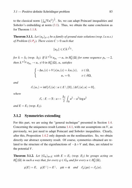
3.1 — Positive definite Schrödinger problem 83
to the classical norm(∫
Ω|∇u|2
) 12 . So, we can adapt Poincaré inequalities and
Sobolev’s embedding at norm (3.1). Thus, we obtain the same conclusion asfor Theorem 1.1.8.
Theorem 3.1.1. Let (up)p>2 be a family of ground state solutions (resp. l.e.n.s.)of Problem (SPp). There exists C > 0 such that
‖up‖6Cλ1
p−2 ,
for λ = λ1 (resp. λ2). If λ1
2−pn upn u∗ in H10 (Ω) for some sequence pn→ 2,
then λ1
2−pn upn → u∗ 6= 0 in H10 (Ω), u∗ satisfies
−∆u∗(x)+V (x)u∗(x) = λu∗(x), x ∈Ω,
u∗ = 0, x ∈ ∂Ω,
andE∗(u∗) = infE∗(u) : u ∈ E \0,〈dE∗(u),u〉= 0,
where
E∗ : E→ R : u 7→ λ2
2
∫Ω
u2−u2 logu2
and E = E1 (resp. E2).
3.1.2 Symmetries extending
For this part, we are using the “general technique” presented in Section 1.4.Concerning the uniqueness result Lemma 1.4.1, with our assumptions on V , aspreviously, we just need to adapt Poincaré and Sobolev inequalities. Clearly,after this, Proposition 1.4.2 only depends on the nonlinearities. So, we obtaindirectly our abstract symmetry result. Of course, symmetries obtained are re-lated to the structure of the eigenfunctions of −∆ +V and, thus, are related tothe potential V .
Theorem 3.1.2. Let (Gα)α∈E with E = E1 (resp. E2) be groups acting onH1
0 (Ω) in such a way that, for every g ∈ Gα and for every u ∈ H10 (Ω),
g(E) = E, g(E⊥) = E⊥, gα = α and Ep(gu) = Ep(u).
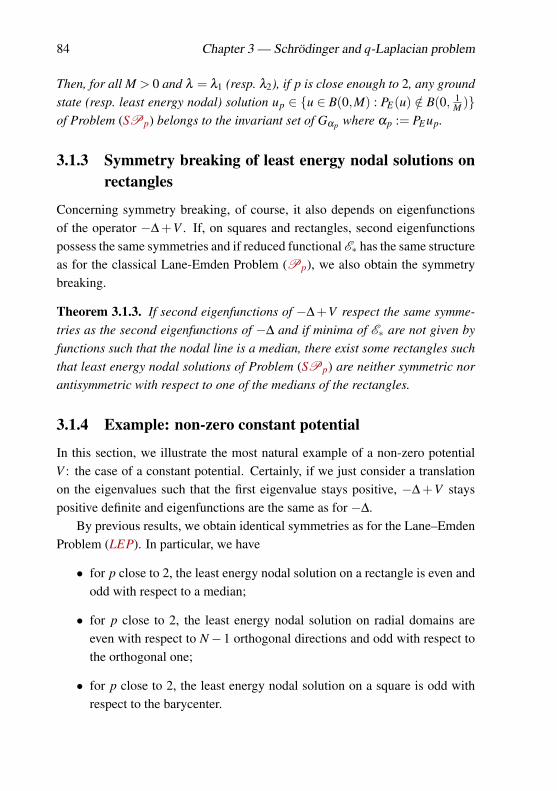
84 Chapter 3 — Schrödinger and q-Laplacian problem
Then, for all M > 0 and λ = λ1 (resp. λ2), if p is close enough to 2, any groundstate (resp. least energy nodal) solution up ∈ u ∈ B(0,M) : PE(u) /∈ B(0, 1
M )of Problem (SPp) belongs to the invariant set of Gαp where αp := PEup.
3.1.3 Symmetry breaking of least energy nodal solutions onrectangles
Concerning symmetry breaking, of course, it also depends on eigenfunctionsof the operator −∆ +V . If, on squares and rectangles, second eigenfunctionspossess the same symmetries and if reduced functional E∗ has the same structureas for the classical Lane-Emden Problem (Pp), we also obtain the symmetrybreaking.
Theorem 3.1.3. If second eigenfunctions of −∆ +V respect the same symme-tries as the second eigenfunctions of −∆ and if minima of E∗ are not given byfunctions such that the nodal line is a median, there exist some rectangles suchthat least energy nodal solutions of Problem (SPp) are neither symmetric norantisymmetric with respect to one of the medians of the rectangles.
3.1.4 Example: non-zero constant potential
In this section, we illustrate the most natural example of a non-zero potentialV : the case of a constant potential. Certainly, if we just consider a translationon the eigenvalues such that the first eigenvalue stays positive, −∆ +V stayspositive definite and eigenfunctions are the same as for −∆.
By previous results, we obtain identical symmetries as for the Lane–EmdenProblem (LEP). In particular, we have
• for p close to 2, the least energy nodal solution on a rectangle is even andodd with respect to a median;
• for p close to 2, the least energy nodal solution on radial domains areeven with respect to N−1 orthogonal directions and odd with respect tothe orthogonal one;
• for p close to 2, the least energy nodal solution on a square is odd withrespect to the barycenter.
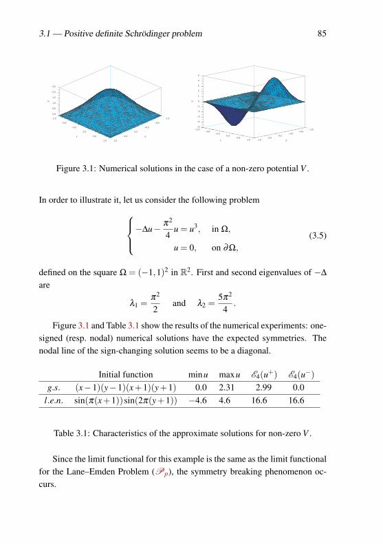
3.1 — Positive definite Schrödinger problem 85
0.0
0.5
1.0
1.5
2.0
2.5
Z
−1.0
−0.6
−0.2
0.2
0.6
1.0
X
−1.0
−0.6
−0.2
0.2
0.6
1.0
Y
−5
−4
−3
−2
−1
0
1
2
3
4
5
Z
−1.0−0.6
−0.20.2
0.61.0 X
−1.0−0.6
−0.20.2
0.61.0Y
Figure 3.1: Numerical solutions in the case of a non-zero potential V .
In order to illustrate it, let us consider the following problem−∆u− π2
4u = u3, in Ω,
u = 0, on ∂Ω,
(3.5)
defined on the square Ω = (−1,1)2 in R2. First and second eigenvalues of −∆
are
λ1 =π2
2and λ2 =
5π2
4.
Figure 3.1 and Table 3.1 show the results of the numerical experiments: one-signed (resp. nodal) numerical solutions have the expected symmetries. Thenodal line of the sign-changing solution seems to be a diagonal.
Initial function minu maxu E4(u+) E4(u−)g.s. (x−1)(y−1)(x+1)(y+1) 0.0 2.31 2.99 0.0
l.e.n. sin(π(x+1))sin(2π(y+1)) −4.6 4.6 16.6 16.6
Table 3.1: Characteristics of the approximate solutions for non-zero V .
Since the limit functional for this example is the same as the limit functionalfor the Lane–Emden Problem (Pp), the symmetry breaking phenomenon oc-curs.
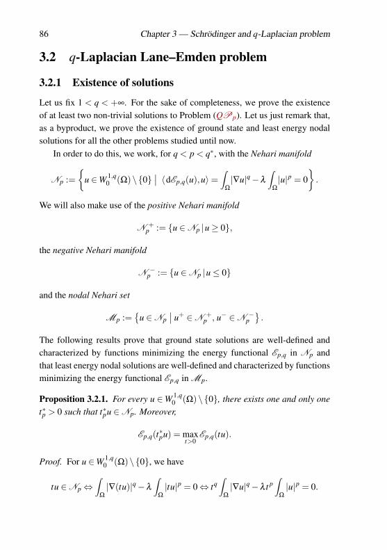
86 Chapter 3 — Schrödinger and q-Laplacian problem
3.2 q-Laplacian Lane–Emden problem
3.2.1 Existence of solutions
Let us fix 1 < q < +∞. For the sake of completeness, we prove the existenceof at least two non-trivial solutions to Problem (QPp). Let us just remark that,as a byproduct, we prove the existence of ground state and least energy nodalsolutions for all the other problems studied until now.
In order to do this, we work, for q < p < q∗, with the Nehari manifold
Np :=
u ∈W 1,q0 (Ω)\0
∣∣ 〈dEp,q(u),u〉=∫
Ω
|∇u|q−λ
∫Ω
|u|p = 0
.
We will also make use of the positive Nehari manifold
N +p := u ∈Np |u≥ 0,
the negative Nehari manifold
N −p := u ∈Np |u≤ 0
and the nodal Nehari set
Mp :=
u ∈Np∣∣ u+ ∈N +
p , u− ∈N −p
.
The following results prove that ground state solutions are well-defined andcharacterized by functions minimizing the energy functional Ep,q in Np andthat least energy nodal solutions are well-defined and characterized by functionsminimizing the energy functional Ep,q in Mp.
Proposition 3.2.1. For every u ∈W 1,q0 (Ω)\0, there exists one and only one
t∗p > 0 such that t∗pu ∈Np. Moreover,
Ep,q(t∗pu) = maxt>0
Ep,q(tu).
Proof. For u ∈W 1,q0 (Ω)\0, we have
tu ∈Np⇔∫
Ω
|∇(tu)|q−λ
∫Ω
|tu|p = 0⇔ tq∫
Ω
|∇u|q−λ t p∫
Ω
|u|p = 0.
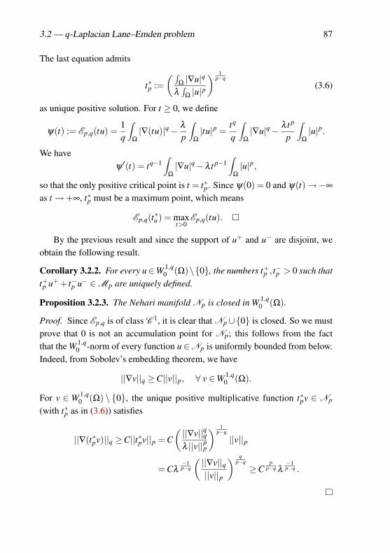
3.2 — q-Laplacian Lane–Emden problem 87
The last equation admits
t∗p :=( ∫
Ω|∇u|q
λ∫
Ω|u|p
) 1p−q
(3.6)
as unique positive solution. For t ≥ 0, we define
ψ(t) := Ep,q(tu) =1q
∫Ω
|∇(tu)|q− λ
p
∫Ω
|tu|p =tq
q
∫Ω
|∇u|q− λ t p
p
∫Ω
|u|p.
We haveψ′(t) = tq−1
∫Ω
|∇u|q−λ t p−1∫
Ω
|u|p,
so that the only positive critical point is t = t∗p. Since ψ(0) = 0 and ψ(t)→−∞
as t→+∞, t∗p must be a maximum point, which means
Ep,q(t∗u ) = maxt>0
Ep,q(tu).
By the previous result and since the support of u+ and u− are disjoint, weobtain the following result.
Corollary 3.2.2. For every u∈W 1,q0 (Ω)\0, the numbers t+p , t−p > 0 such that
t+p u+ + t−p u− ∈Mp are uniquely defined.
Proposition 3.2.3. The Nehari manifold Np is closed in W 1,q0 (Ω).
Proof. Since Ep,q is of class C 1, it is clear that Np∪0 is closed. So we mustprove that 0 is not an accumulation point for Np; this follows from the factthat the W 1,q
0 -norm of every function u ∈Np is uniformly bounded from below.Indeed, from Sobolev’s embedding theorem, we have
||∇v||q ≥C||v||p, ∀ v ∈W 1,q0 (Ω).
For v ∈W 1,q0 (Ω) \ 0, the unique positive multiplicative function t∗pv ∈ Np
(with t∗p as in (3.6)) satisfies
||∇(t∗pv)||q ≥C||t∗pv||p = C(||∇v||qqλ ||v||pp
) 1p−q
||v||p
= Cλ−1p−q
(||∇v||q||v||p
) qp−q
≥Cp
p−q λ−1p−q .
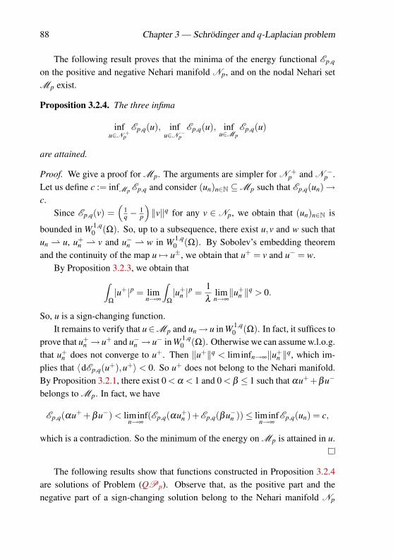
88 Chapter 3 — Schrödinger and q-Laplacian problem
The following result proves that the minima of the energy functional Ep,q
on the positive and negative Nehari manifold Np, and on the nodal Nehari setMp exist.
Proposition 3.2.4. The three infima
infu∈N +
p
Ep,q(u), infu∈N −
p
Ep,q(u), infu∈Mp
Ep,q(u)
are attained.
Proof. We give a proof for Mp. The arguments are simpler for N +p and N −
p .Let us define c := infMp Ep,q and consider (un)n∈N ⊆Mp such that Ep,q(un)→c.
Since Ep,q(v) =(
1q −
1p
)‖v‖q for any v ∈ Np, we obtain that (un)n∈N is
bounded in W 1,q0 (Ω). So, up to a subsequence, there exist u,v and w such that
un u, u+n v and u−n w in W 1,q
0 (Ω). By Sobolev’s embedding theoremand the continuity of the map u 7→ u±, we obtain that u+ = v and u− = w.
By Proposition 3.2.3, we obtain that∫Ω
|u+|p = limn→∞
∫Ω
|u+n |p =
1λ
limn→∞‖u+
n ‖q > 0.
So, u is a sign-changing function.It remains to verify that u∈Mp and un→ u in W 1,q
0 (Ω). In fact, it suffices toprove that u+
n → u+ and u−n → u− in W 1,q0 (Ω). Otherwise we can assume w.l.o.g.
that u+n does not converge to u+. Then ‖u+‖q < liminfn→∞‖u+
n ‖q, which im-plies that 〈dEp,q(u+),u+〉 < 0. So u+ does not belong to the Nehari manifold.By Proposition 3.2.1, there exist 0 < α < 1 and 0 < β ≤ 1 such that αu+ +βu−
belongs to Mp. In fact, we have
Ep,q(αu+ +βu−) < liminfn→∞
(Ep,q(αu+n )+Ep,q(βu−n ))≤ liminf
n→∞Ep,q(un) = c,
which is a contradiction. So the minimum of the energy on Mp is attained in u.
The following results show that functions constructed in Proposition 3.2.4are solutions of Problem (QPp). Observe that, as the positive part and thenegative part of a sign-changing solution belong to the Nehari manifold Np
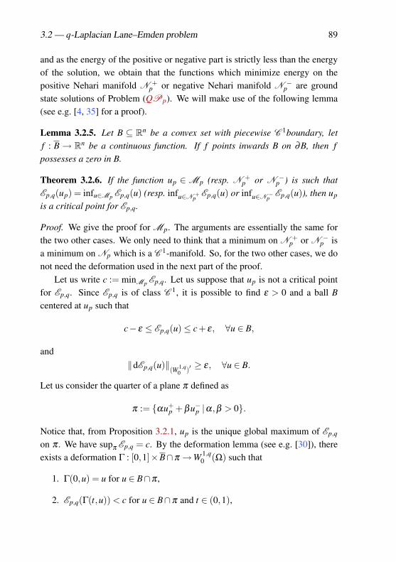
3.2 — q-Laplacian Lane–Emden problem 89
and as the energy of the positive or negative part is strictly less than the energyof the solution, we obtain that the functions which minimize energy on thepositive Nehari manifold N +
p or negative Nehari manifold N −p are ground
state solutions of Problem (QPp). We will make use of the following lemma(see e.g. [4, 35] for a proof).
Lemma 3.2.5. Let B ⊆ Rn be a convex set with piecewise C 1boundary, letf : B→ Rn be a continuous function. If f points inwards B on ∂B, then fpossesses a zero in B.
Theorem 3.2.6. If the function up ∈Mp (resp. N +p or N −
p ) is such thatEp,q(up) = infu∈Mp Ep,q(u) (resp. infu∈N +
pEp,q(u) or infu∈N −
pEp,q(u)), then up
is a critical point for Ep,q.
Proof. We give the proof for Mp. The arguments are essentially the same forthe two other cases. We only need to think that a minimum on N +
p or N −p is
a minimum on Np which is a C 1-manifold. So, for the two other cases, we donot need the deformation used in the next part of the proof.
Let us write c := minMp Ep,q. Let us suppose that up is not a critical pointfor Ep,q. Since Ep,q is of class C 1, it is possible to find ε > 0 and a ball Bcentered at up such that
c− ε ≤ Ep,q(u)≤ c+ ε, ∀u ∈ B,
and‖dEp,q(u)‖(W 1,q
0 )′ ≥ ε, ∀u ∈ B.
Let us consider the quarter of a plane π defined as
π := αu+p +βu−p |α,β > 0.
Notice that, from Proposition 3.2.1, up is the unique global maximum of Ep,q
on π . We have supπ Ep,q = c. By the deformation lemma (see e.g. [30]), thereexists a deformation Γ : [0,1]×B∩π →W 1,q
0 (Ω) such that
1. Γ(0,u) = u for u ∈ B∩π ,
2. Ep,q(Γ(t,u)) < c for u ∈ B∩π and t ∈ (0,1),
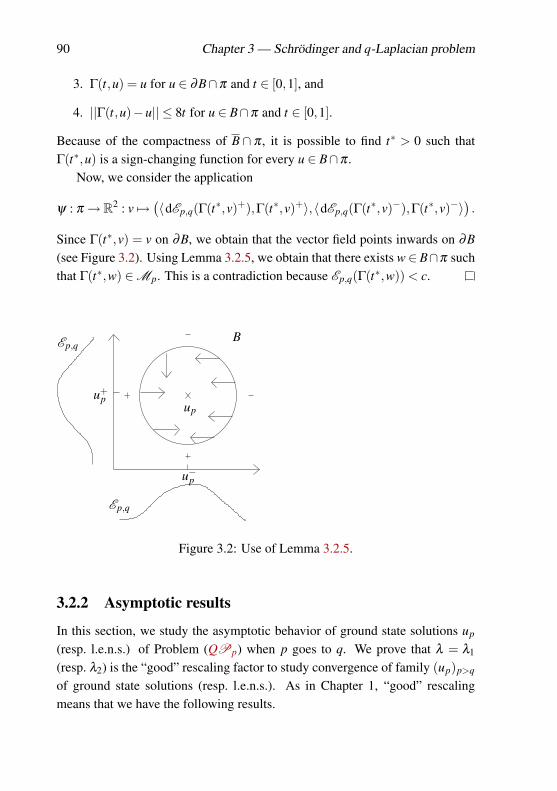
90 Chapter 3 — Schrödinger and q-Laplacian problem
3. Γ(t,u) = u for u ∈ ∂B∩π and t ∈ [0,1], and
4. ||Γ(t,u)−u|| ≤ 8t for u ∈ B∩π and t ∈ [0,1].
Because of the compactness of B∩ π , it is possible to find t∗ > 0 such thatΓ(t∗,u) is a sign-changing function for every u ∈ B∩π .
Now, we consider the application
ψ : π→R2 : v 7→(〈dEp,q(Γ(t∗,v)+),Γ(t∗,v)+〉,〈dEp,q(Γ(t∗,v)−),Γ(t∗,v)−〉
).
Since Γ(t∗,v) = v on ∂B, we obtain that the vector field points inwards on ∂B(see Figure 3.2). Using Lemma 3.2.5, we obtain that there exists w∈ B∩π suchthat Γ(t∗,w) ∈Mp. This is a contradiction because Ep,q(Γ(t∗,w)) < c.
u−p
u+p
Ep,q
Ep,q
up
B
Figure 3.2: Use of Lemma 3.2.5.
3.2.2 Asymptotic results
In this section, we study the asymptotic behavior of ground state solutions up
(resp. l.e.n.s.) of Problem (QPp) when p goes to q. We prove that λ = λ1
(resp. λ2) is the “good” rescaling factor to study convergence of family (up)p>q
of ground state solutions (resp. l.e.n.s.). As in Chapter 1, “good” rescalingmeans that we have the following results.
3.2 — q-Laplacian Lane–Emden problem 91
Theorem 3.2.7. As p→ q, ground state solutions up of Problem (QPp)(i) diverge to infinity if λ < λ1;(ii) converge to a non-zero first eigenfunction of the q-Laplacian, up to a subse-quence, if λ = λ1;(iii) converge to zero if λ > λ1.
Theorem 3.2.8. As p→ q, least energy nodal solutions up of Problem (QPp)(i) diverge to infinity if λ < λ2;(ii) converge to a non-zero second eigenfunction of the q-Laplacian, up to asubsequence, if λ = λ2;(iii) converge to zero if λ > λ2.
In fact, we have that there exist suitable positive constants C1 and C2 suchthat
C1
(λ1
λ
) 1p−q
≤ ‖up‖ ≤C2
(λ1
λ
) 1p−q
if up is a ground state solution, and
C1
(λ2
λ
) 1p−q
≤ ‖up‖ ≤C2
(λ2
λ
) 1p−q
if up is a least energy nodal solution.Let us mention that the case λ < λ1 in Theorem 3.2.7 was already investi-
gated in [42].
Let us first remark that statements (i) and (iii) of Theorems 3.2.7 and 3.2.8can directly be derived from (ii) as follows. If vp is a ground state solution
of Problem (QPp) with λ = λ1, then up :=(
λ1µ
) 1p−q
vp will be a ground state
solution for λ = µ . So for λ < λ1, as p > q and p→ q, up :=(
λ1λ
) 1p−q
vp goesto infinity, while for λ > λ1 it goes to zero. The proof of Theorem 3.2.8 (i) and(iii) is virtually identical. It remains to study (ii). We consider the case λ =λ1 (resp. λ2) for ground state (resp. least energy nodal) solutions. The family(up,1)p>q will denote a family of ground state solutions for the problem (QPp)with λ = λ1, while (up,2)p>q will be a family of least energy nodal solutionsfor the same problem with λ = λ2.
92 Chapter 3 — Schrödinger and q-Laplacian problem
The process is more or less the same as in Chapter 1. In the proofs, wejust point out the differences with the linear case when q = 2. Let us fix a firstnon-zero eigenfunction e1 and a non-zero second eigenfunction e2 of −∆q.
Lemma 3.2.9. For q < r < q∗, the quantities supq<p<r t∗p, supq<p<r t+p andsupq<p<r t−p are finite, where t∗p, t+p and t−p are the unique positive real num-bers such that t∗pe1 ∈Np and t+p e+
2 + t−p e−2 ∈Mp.
Proof. The proof is exactly the same as for Lemma 1.1.1.
Proposition 3.2.10. The families (up,1)p>q and (up,2)p>q are uniformly boun-
ded in W 1,q0 (Ω).
Proof. Again, the proof is the same as for Proposition 1.1.2.
About Proposition 1.1.3, as we need the Fredholm alternative, we cannotwork in the same way. The two following results prove that the sequence ofground state solutions (resp. least energy nodal solutions) of Problem (QPp)stays away from zero.
Proposition 3.2.11. Let(uq,1)
q>p be a family of ground state solutions of Prob-lem (QPp) for λ = λ1. Then
liminfp→q
||∇up,1||q > 0.
Proof. We are working in the same vein as Proposition 1.1.6. In fact, thestudy of ground state solutions simplifies the arguments. We do not need touse Lemma 1.1.5 and we directly can use the Hölder inequality on the groundstate solutions.
Concerning least energy nodal solutions, we cannot use the Poincaré in-equality as in Proposition 1.1.6. To solve this problem, we use the Krasnoselskiigenus 3.3 defined in the Introduction of this chapter.
Proposition 3.2.12. Let (up,2)p>q be a family of least energy nodal solutions ofProblem (QPp) for λ = λ2. Then
liminfp→q
||∇up,2||q > 0.
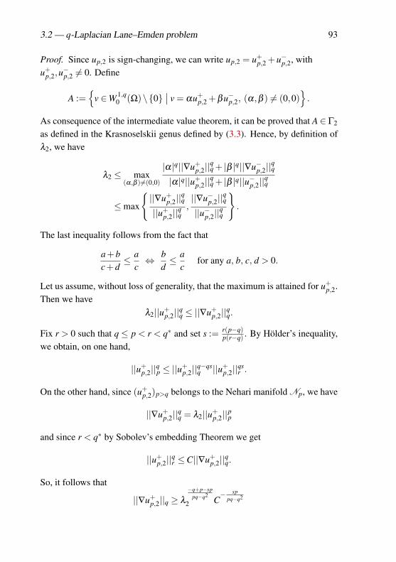
3.2 — q-Laplacian Lane–Emden problem 93
Proof. Since up,2 is sign-changing, we can write up,2 = u+p,2 +u−p,2, with
u+p,2,u
−p,2 6= 0. Define
A :=
v ∈W 1,q0 (Ω)\0
∣∣ v = αu+p,2 +βu−p,2, (α,β ) 6= (0,0)
.
As consequence of the intermediate value theorem, it can be proved that A ∈ Γ2
as defined in the Krasnoselskii genus defined by (3.3). Hence, by definition ofλ2, we have
λ2 ≤ max(α,β )6=(0,0)
|α|q||∇u+p,2||
qq + |β |q||∇u−p,2||
|α|q||u+p,2||
qq + |β |q||u−p,2||
≤max
||∇u+
p,2||qq
||u+p,2||
,||∇u−p,2||
||u−p,2||qq
.
The last inequality follows from the fact that
a+bc+d
≤ ac⇔ b
d≤ a
cfor any a, b, c, d > 0.
Let us assume, without loss of generality, that the maximum is attained for u+p,2.
Then we haveλ2||u+
p,2||qq ≤ ||∇u+
p,2||qq.
Fix r > 0 such that q≤ p < r < q∗ and set s := r(p−q)p(r−q) . By Hölder’s inequality,
we obtain, on one hand,
||u+p,2||
qp ≤ ||u+
p,2||q−qsq ||u+
p,2||qsr .
On the other hand, since (u+p,2)p>q belongs to the Nehari manifold Np, we have
||∇u+p,2||
qq = λ2||u+
p,2||pp
and since r < q∗ by Sobolev’s embedding Theorem we get
||u+p,2||
qr ≤C||∇u+
p,2||qq.
So, it follows that
||∇u+p,2||q ≥ λ
−q+p−sppq−q2
2 C− sp
pq−q2
94 Chapter 3 — Schrödinger and q-Laplacian problem
and, putting in the value of s,
||∇u+p,2||q ≥ λ
1q−r
2 Cr
q(q−r) .
From the relation||∇up,2||q ≥ ||∇u+
p,2||q
and since the estimate does not depend on p, we obtain the claim.
Theorem 3.2.13. Let (up,1)p>q be a family of ground state solutions of Prob-lem (QPp) for λ = λ1 (resp. (up,2)p>q be a family of least energy nodal solu-tions for λ = λ2). Then, up to a subsequence, up,1 → u∗ (resp. up,2 → u∗) inLq(Ω) as p→ q, where the function u∗ is a non-zero first (resp. second) eigen-function of the q-Laplacian.
Proof. We give the proof for the family of least energy nodal solutions. Theidea is the same for the family of ground state solutions. Let v ∈W 1,q
0 (Ω).Because of the uniform boundedness of the (up,2)p>q in W 1,q
0 (Ω), there existsu∗ ∈W 1,q
0 (Ω) such that up,2 u∗ in W 1,q0 (Ω) and up,2→ u∗ in Lq(Ω) for p→ q
(up to a subsequence). By Lebesgue’s dominated convergence theorem we alsohave
|up,2|p−2up,2→ |u∗|q−2u∗ in Lq(Ω).
So, ∫Ω
|∇u∗|q−2∇u∗∇v = lim
p→q
∫Ω
|∇up,2|q−2∇up,2∇v
= limp→q
λ2
∫Ω
|up,2|p−2up,2v
= λ2
∫Ω
|u∗|q−2u∗v.
By Theorem 3.2.12, u∗ 6= 0. Hence, u∗ is a non-zero second eigenfunction of−∆q.
Chapter 4
General nonlinearities
In this chapter, we consider some perturbations of fp(x) = |x|p−2x, the non-linearity studied for the Lane–Emden Problem (Pp) with DBC in Chapter 1.We work with Problem (GPp)
−∆u = fp(u), in Ω,
u = 0, on ∂Ω,(GPp)
where Ω is an open bounded connected domain of RN , N > 2, 2 < p < 2∗,fp(0) = 0 and fp ∈ C 1(R). We are interested in non-necessarily homogeneousnonlinearities and we would like to know whether results given in Chapter 1are still valid or not.
Under some growth assumptions, the solutions of Problem (GPp) are thecritical points of the energy functional
Ep : H10 (Ω)→ R : u→ 1
2
∫Ω
|∇u|2−∫
Ω
Fp(u),
where Fp(t) :=∫ t
0 fp(s)ds. To explain this, let us denote M(R) the set of Borel-measurable functions from R to R. For a function h∈M(R) and positive reals qand γ , we refer respectively to a polynomial or an exponential growth conditionby
(PGq) there exists C > 0,∀t ∈ R, |h(t)|6C(|t|q +1);
95
96 Chapter 4 — General nonlinearities
(EGγ) there exists C > 0,∀t ∈ R, |h(t)|6Ceγ t2.
The classical subcritical and exponential growth assumptions are defined as
(GA1) for all p > 2,∃ q ∈ (2,2∗) such that fp satisfies (PGq−1);
(GA′1) for all p > 2,∃0 < γ < γ0 such that fp satisfies (EGγ).
The condition (GA1) is motivated by the classical Sobolev embedding theoremwhile the latter is related to the Trudinger-Moser inequality when N = 2: forall γ > 0 and all u ∈ H1(Ω),
∫Ω
eγu2< +∞ and, moreover, there exists γ0 =
γ0(Ω) > 0 such that
sup∫
Ω
eγu2: ‖u‖6 1
< +∞
if and only if γ < γ0 [52]. These assumptions ensure that the energy functionalEp is well-defined and of class C 1(Ω) on H1
0 (Ω) (see e.g. [35]). Let us alsonote that in the case of assumption (GA′1) in dimension 2, the following lemma,proved in [15], plays the role of the standard compactness argument when as-suming a subcritical polynomial growth.
Lemma 4.0.14. Let un,vn ∈H1(Ω) such that ‖un‖,‖vn‖6 1. If un u,vn vin H1(Ω) and γn → γ < γ0, then, for every p ∈ [1,+∞) and every q ∈ [1, γ0
γ),
vpneγnu2
n → vpeγu2in Lq(Ω).
To obtain the existence of non-zero solutions, we consider the followingstandard assumption (GA2) giving a mountain pass structure (see Figure 1.1 inChapter 1) to the functional Ep with a Nehari fibering method.
(GA2) (a) For all p > 2, limt→0fp(t)|t| = 0;
(b) for all p > 2, lim|t|→∞
fp(t)t = +∞;
(c) for all p > 2,∀t 6= 0,(
fp(t)|t|
)′> 0.
As in Chapter 1, we define the Nehari manifold Np (resp. the nodal Nehariset Mp) as
Np :=
u ∈ H10 (Ω)\0
∣∣ ‖u‖2 =∫
Ω
fp(u)u
97
(resp.Mp :=
u ∈ H1
0 (Ω) : u± ∈Np).
Under the assumptions (GA1)− (GA2), J. Van Schaftingen and M. Willem ob-tained in [68] the existence of ground state and least energy nodal solutions.Ground state (resp. least energy nodal) solutions are the critical points of Ep
with minimum energy on Np (resp. Mp). They generalized the existence re-sult of A. Castro, J. Cossio and J. M. Neuberger where additional assumptions(like the super-quadraticity (AA1) here under) were required (see e.g. [23] orProposition 3.2.6).
We will always suppose that either assumptions (GA1)−(GA2) hold or N =2 and (GA′1)− (GA2) hold.
To obtain expected asymptotic behavior of a family of ground state solutions(resp. l.e.n.s.) (up)p>2, see Section 1.1, we work in Section 4.1 with the classicalsuper-quadraticity assumption (AA1).
(AA1) For all p > 2,∀t ∈ R, fp(t)t > pFp(t).
In some sense, we are working with a family of problems parametrized by super-quadraticity constants. Assumption (AA1) implies that |Fp| is comparable to |t|p
and ensures that if u ∈Np, then
Ep(u) =12‖u‖2−
∫Ω
Fp(u)>12‖u‖2− 1
p
∫Ω
fp(u)u =(
12− 1
p
)‖u‖2. (4.1)
Moreover, we need the following assumption (AA2). Like usual, λ1 (resp. λ2)defined in (AA2)(a) will be used for ground state solutions (resp. l.e.n.s.).
(AA2) (a) For all t ∈ R, limp→2 fp(t) =: f2(t) = λ t, for some λ ∈ λ1, λ2,and, for all t0 ∈ R, lim(p,t)→(2,t0)
fp(t)− f2(t)p−2 =: f∗(t0) ∈ R;
(b) if fp satisfies (GA1) (resp. (GA′1)), there exist q ∈ (2,2∗) (resp. γ >
0) and h ∈M(R) verifying (PGq) (resp. (EGγ)) such that, for anyp > 2,∀t ∈ R, | fp(t)|6 h(t);
(c) there exist q ∈ [2,2∗] (resp. γ > 0) and h ∈M(R) verifying
(PGq−1) (resp. (EGγ)) such that∣∣∣ fp(t)− f2(t)
p−2
∣∣∣6 h(t), for all p closeto 2 and t ∈ R;
(d) (i) limt→0f∗(t)
t < 0, (ii) lim|t|→∞
f∗(t)t > 0, (iii) t 7→ f∗(t)
|t| increasing.
98 Chapter 4 — General nonlinearities
Roughly, it mainly means
fp(t) = λ t + f∗(t)(p−2)+gp(t), (4.2)
where gp(t) behaves like o(p− 2). These assumptions permit us to define thereduced functional
E∗ : E→ R : u 7→ −∫
Ω
F∗(u), where F∗(t) :=∫ t
0f∗(s)ds,
and E is the eigenspace of −∆ with DBC related to λ . We also define theassociated reduced Nehari manifold
N∗ := u ∈ E \0 : 〈dE∗(u),u〉= 0.
One can easily check that E∗ is well-defined and does have a mountain passgeometry. These assumptions also imply that any weak accumulation point u∗of (up)p>2 is a critical point of the functional E∗. We obtain the boundedness of(up)p>2 under the assumptions (AA1)− (AA3).
(AA3) (a) For all t0 ∈ R, lim(p,t)→(2,t0)f ′p(t)t2− fp(t)t
p−2 =: H∗(t0);
(b) there exist q ∈ [2,2∗] (resp. γ > 0) and h ∈M(R) verifying(PGq−1) (resp. (EGγ)) such that,
∀p > 2, ∀t ∈ R,∣∣∣ f ′p(t)t− fp(t)
p−2
∣∣∣6 h(t);
(c) there exists a critical point u∗ of E∗ such that∫
ΩH∗(u∗) 6= 0.
Roughly, it mainly means that u∗ is an nondegenerate critical point of E∗. Letus also note that (AA2)(a) and (AA3)(a) can be rephrased as a convergence inp locally uniform with respect to t.
If u∗ is a weak accumulation point of (up)p>2, then it is different from 0under the assumption (AA2) and (AA4) (resp. (AA′4)). Let us remark that we donot need anymore the assumption (AA3) (resp. (AA2) and (AA3)).
(AA4) There exists η > 0 s.t., ∀p < 2 + η and ∀t ∈ (−η ,η) \ 0, fp(t)t < λ .
Moreover, Ω is a domain of class C 2 (or a product of intervals).
(AA′4) There exists q ∈ (2,2∗),∀p > 2,∃c1(p),c2(p) > 0,
99
∀t ∈ R, | fp(t)|6 λ |t|1+c1(p) + c2(p)|t|q−1,
with limp→2 ci(p) = 0 and ∃k ∈ R,∀p > 2, log(1−c2(p))c1(p) > k,
This assumption (AA4) is the uniform version of assumption (GA2)(a). Insome sense, assumption (AA4) is more general than assumption (AA′4) but re-quires some smooth conditions on ∂Ω to obtain a C -convergence of up (seeRemark 2.1.5).
To obtain the expected symmetries (see Section 1.4), we give in Section 4.2assumptions implying, in any ball of H1
0 (Ω), the uniqueness of solutions up tothe projection on some eigenspace E. Let us remark that we are more generalthan in Chapter 1 in the sense that solutions are not necessarily ground state orleast energy nodal solutions and the eigenfunctions are not necessarily the firstor second ones. To do it, we consider assumptions (SA1) and (SA2) (or (SA′2)).Assumption (SA1) replaces some parts of the assumption (AA2).
(SA1) (a) For all t0 ∈ R : limp→2,t→t0 fp(t) =: f2(t0) = λ t0, for some eigen-value λ of −∆ in H1
0 (Ω);
(b) if fp satisfies (GA1) (resp. (GA′1)), there exist q ∈ (2,2∗) (resp. γ >
0) and h ∈ M(R) verifying (PGq) (resp. (EGγ)) such that, ∀p >
2,∀t ∈ R, | fp(t)|6 h(t).
(SA2) (a) For all u0 6= 0, lim(s,t,p)→(uo,uo,2)fp(s)− fp(t)
t−s = λ ;
(b) there exist q ∈ [2,2∗] and ha,hb ∈ M(R) verifying (PGq−2) suchthat, for every p > 2 and all s 6= t ∈ R,∣∣∣ fp(t)− fp(s)
t−s
∣∣∣6 ha(s)+hb(t).
(SA′2) (a) For all u0 6= 0, lim(s,t,p)→(uo,uo,2)fp(s)− fp(t)
t−s = λ ;
(b) there exist γ > 0 and ha,hb ∈M(R) verifying (EGγ) such that, forevery p > 2 and all s 6= t ∈ R,∣∣∣ fp(t)− fp(s)
t−s
∣∣∣6 ha(s)+hb(t).
In assumption (SA1)(a), we suppose that the limit of fp(t) is λ t, with λ beingprecisely an eigenvalue (not necessarily λ1 or λ2). When looking at the Lane–Emden equation (Pp), one easily understands that this is not restrictive (see
100 Chapter 4 — General nonlinearities
Theorems 3.2.7 and 3.2.8). At least heuristically, one can see that if λ 6= λi,any converging sequence of solutions goes to either zero or infinity. That is whywe have systematically studied the renormalized equation. Let us just remarkthat, with general nonlinearities, a changement of λ could change symmetriesof solutions. Under (SA1) and (SA2), we obtain that if a bounded family ofsolutions (up)p>2 is staying away from zero, for p close enough to 2, up respectsthe symmetries of its projection on the eigenspace E associated with λ .
As for the Lane–Emden Problem (Pp) with a homogeneous nonlinearity(see Section 1.5), it is worth pointing out that symmetry results are not uniformwith respect to the domain. Namely, we are able to build rectangles close to thesquare where least energy nodal solutions are neither symmetric nor antisym-metric with respect to the medians of the rectangles.
Let us just note that there exist non homogeneous nonlinearities respectingall the previous assumptions. We will analyze in Section 4.3 the three followingcases for fp:
λ t|t|p−2 +(p−2)t|t|q−2, λ t(et2 −1)p−2 and λ t
(k
∑i=1
αi|t|βi(p)
),
i.e. the case of a subcritical superlinear (2 < q < 2∗) perturbation of a slowlygrowing homogeneous superlinearity, of a slowly exponentially growing sub-critical nonlinearity in dimension two, and of a sum of small powers. Thesecases will be numerically illustrated.
To finish, in Section 4.4, we provide another “geometrical” assumptionreplacing (AA1) and (AA3) and implying the boundedness of the families ofground state solutions and least energy nodal solutions in H1
0 (Ω). We basicallyintroduce a super-lower homogeneity assumption.
This work is inspired by the paper [12] written in collaboration with D. Bon-heure and V. Bouchez.
4.1 Asymptotic behavior
In this section, we work out a priori estimates for ground state and least energynodal solutions, and we analyze their asymptotic behavior when p→ 2. In
4.1 — Asymptotic behavior 101
the sequel of this section, λ exclusively takes the value λ1, when we discussground state solutions, and λ2 when we deal with least energy nodal solutions.The space E will denote the eigenspace of −∆ with DBC related to λ .
4.1.1 Limit equation
We turn our attention to the candidate accumulation points of (up)p>2, as p→ 2.The following result generalizes Lemma 1.1.7.
Lemma 4.1.1. Let (up)p>2 be a bounded family of ground state (resp. leastenergy nodal) solutions of Problem (GPp). If pn→ 2 and upn u∗ in H1
0 (Ω),then, under assumptions (GA1)−(GA2) and (AA2)−(AA3), upn→ u∗ in H1
0 (Ω)and u∗ solves
−∆u∗ = λu∗, in Ω,
u∗ = 0, on ∂Ω,∫Ω
f∗(u∗)v = 0, ∀v ∈ E.
Proof. The proof is similar as Lemma 1.1.7. By assumption (AA2), we obtainthat
fpn(upn)→ f2(u∗) in L2(Ω), so that∫
Ω
∇u∗∇v = λ
∫Ω
u∗v.
Then, by using Lebesgue’s dominated convergence theorem and (AA3), we ob-tain
0 = limn→∞
∫Ω
( fpn(upn)−λupn)vpn−2
= λ
∫Ω
f∗(u∗)v.
About the convergence in H10 (Ω), we have∫
Ω
|∇up−∇u∗|2 =∫
Ω
|∇up|2−2∫
Ω
∇up∇u∗+∫
Ω
|∇u∗|2
=∫
Ω
fp(up)up−2∫
Ω
∇up∇u∗+λ
∫Ω
u2∗
which converges to λ∫
Ωu2∗−2
∫Ω
∇u∗∇u∗+λ∫
Ωu2∗ = 0.
4.1.2 Upper bound
To obtain an upper bound, we construct appropriate test functions leading to anestimate of the energy and the norm of ground state solutions (resp. l.e.n.s.) of
102 Chapter 4 — General nonlinearities
Problem (GPp) (as in Proposition 1.1.3). Let us consider a family (vp)p>2 ∈H1
0 (Ω)\0 and
hp : (0,+∞)→ R : t 7→∫
Ω
t−1 fp(tvp)vp.
This last function is well-defined because of assumption (GA2). Moreover, hp
is continuous, increasing and limt→+∞ hp(t) = +∞. Let us denote by h−1p the
inverse of hp. In the next statement, we denote by vp the classical projection ofvp on Np along rays, which is characterized by
vp = tpvp, where hp(tp) = ‖vp‖2.
The next lemma generalizes Proposition 1.1.3. To understand well wherethe assumptions are playing a role, we give the entire proof.
Lemma 4.1.2. Let vp := v∗+(p− 2)w, where w is the unique function in E⊥
verifying −∆w−λw = f∗(v∗), in Ω,
w = 0, on ∂Ω,
and v∗ is a critical point of E∗ such that∫
ΩH∗(v∗) 6= 0. Then, under assumptions
(GA1)− (GA2) and (AA2)− (AA3), the family (vp)p>2 converges to v∗.
Proof. We focus on the case λ = λ1. We need to prove that tp → 1. By theFredholm alternative, w is well-defined. We then compute
‖vp‖2 =∫
Ω
(λv∗+λ (p−2)w+(p−2) f∗(v∗))vp
=∫
Ω
(λvp +(p−2) f∗(v∗))vp
=∫
Ω
fp(vp)vp +(p−2)(∫
Ω
λvp− fp(vp)p−2
vp +∫
Ω
f∗(v∗)vp
)=∫
Ω
fp(vp)vp +(p−2)mp,
where, by (AA2), mp → 0, as p→ 2. We therefore deduce, thanks to (GA2),that
tp = h−1p
(∫Ω
fp(vp)vp +(p−2)mp
).
4.1 — Asymptotic behavior 103
By defining kp :=∫
Ωfp(vp)vp, we have h−1
p (kp) = 1. So, we need to prove that
limp→2
h−1p (kp +mp(p−2))−h−1
p (kp) = 0.
It is true since
dthp(t) =∫
Ω
t−1 f ′p(tvp)v2p− t−2 fp(tvp)vp (4.3)
and (p−2)(h−1p )′ is uniformly bounded (with respect to p) in a neighbourhood
of kp. In fact, let us split the last expression as follows(h−1
p (kp +o(p−2))−h−1p (kp)
o(p−2)− (h−1
p )′(kp)+(h−1p )′(kp)
)o(p−2).
To prove that the first part of the sum converges to 0, we only need to prove thatthe coefficient in front of o(p−2) is uniformely bounded in p. Observe that thedifferentiability of hp at 1 without control on p is not sufficient. So, let us provethat hp is uniformely derivable in p at 1. This is true because lim(p,t)→(0,1) h′p(t)exists, implied by Lebesgue’s dominated convergence theorem jointed to as-sumption (AA3) and (4.3).
For the second part, it is sufficient to prove that (h−1p )′(kp)(p−2) is boun-
ded, i.e.h′p(1)p−2 is away from 0. This is clear since, by assumption (AA3), it
converges to∫
ΩH∗(v∗) which is different from zero.
We now deduce from the previous Lemma 4.1.2 the desired upper bound.We explain how just an inequality between energy and norm given by the super-quadraticity assumption (AA1) is enough.
Theorem 4.1.3. Let (up)p>2 be a family of ground state (resp. least energynodal) solutions of Problem (GPp). Then, under assumptions (GA1)− (GA2)and (AA1)− (AA3), the family (up)p>2 is bounded and if upn u∗ for somesequence pn→ 2, then we have
limn→∞
(Epn(upn)
pn−2
)= E∗(u∗)6 E∗(v∗),
for any critical point v∗ of the functional E∗ such that∫
ΩH∗(v∗) 6= 0.
104 Chapter 4 — General nonlinearities
Proof. Let us consider the family (vp)p>2 given in Lemma 4.1.2. We have that‖vp‖2 = λ‖vp‖2
2 +o(p−2). Indeed, using assumption (AA2), we infer
‖vp‖2−∫
Ωf2(vp)vp
p−2=∫
Ω
fp(vp)− f2(vp)p−2
vp→∫
Ω
f∗(v∗)v∗ = 0,
when p→ 2.So,
Ep(vp)p−2
=
∫Ω(λ
2 v2p−Fp(vp))p−2
+o(1)−−−→p→2
E∗(v∗),
where the last convergence is due to (AA2) and to the definitions of Fp and F∗.Inequality (4.1) given by assumption (AA1) ensures the boundedness of
(up)p>2 and hence the weak convergence up to a subsequence. As observedin Lemma 4.1.1, the convergence is strong. Notice also that
‖up‖2 = λ‖up‖22 +o(p−2).
Indeed, using assumption (AA2) and Lemma 4.1.1, we infer
‖up‖2−∫
Ωf2(up)up
p−2=∫
Ω
fp(up)− f2(up)p−2
up→∫
Ω
f∗(u∗)u∗ = 0,
when p→ 2. Hence, arguing as for the sequence (vp)p>2, we infer that
limn→∞
Epn(upn)pn−2
= E∗(u∗)
and, by definition of (upn)n∈N, we have Epn(upn) 6 Epn(vpn). This ends theproof.
Remark 4.1.4. Assumption (AA2) essentially ensures that we can write
fp(t) = λ t + f∗(t)(p−2)+gp(t)
where gp(·) = o(p− 2). Then, if we rewrite the quotientf ′p(t)t2− fp(t)t
p−2 havingthis in mind, we obtain that a natural sufficient condition for (AA3) to hold isthat g′p(·) = o(p−2) as well. In this case, the function H∗ turns out to be
f ′∗(t)t2− f∗(t)t
4.1 — Asymptotic behavior 105
and since u∗ ∈N∗, the condition∫
ΩH∗(u∗) 6= 0 is equivalent to
∫Ω
f ′∗(u∗)u2∗ 6= 0
which implies that the second derivative of the energy at u∗ in its own directionsis not zero. This last condition is the natural starting point of an approach basedon the implicit function theorem (see page 34) to ensure the existence of a con-tinuum of solutions of Problem (GPp) emanating from u∗. Let us emphasizethat the arguments in this remark are very rough: we have to suppose f∗ to bederivable, while in some simple model example, it is not the case everywhereon R.
4.1.3 Lower bound
We now consider two sets of conditions which ensure that the accumulationpoints u∗ of (up)p>2 are different from 0. For the first theorem using assump-tion (AA4), we need the following property, which has its own interest, aboutthe optimal constant of the Poincaré’s inequality. In any way, it is using theidea given in Chapter 3 when we are working with the q-Laplacian (see Propo-sition 3.2.12). We are using the “linear” version of the Krasnoselskii genus 3.3,namely Riesz-Fisher characterization.
Proposition 4.1.5. If u ∈ H10 (Ω), then λ2
∫Ω(u+)2 6 ‖u+‖2 or λ2
∫Ω(u−)2 6
‖u−‖2.
Proof. W.l.o.g., we can assume that u+ 6= 0 and u− 6= 0. By the Riesz-Fishercharacterization of λ2, we have
λ2 = infdimF=2
supu∈F\0
‖u‖2∫Ω|u|2
.
If we define
F :=
v ∈ H10 (Ω)
∣∣ v = αu+ +βu−, α, β ∈ R
,
then
λ2 6 max(α,β )6=(0,0)
α2‖u+‖2 +β 2‖u−‖2
α2‖u+‖22 +β 2‖u−‖2
2= max
‖u+‖2
‖u+‖22,‖u−‖2
‖u−‖22
ensuring the thesis.
106 Chapter 4 — General nonlinearities
In Chapter 2, Section 2.1, we studied the C -convergence of a sequenceof least energy nodal solutions. The arguments were presented for the Lane-Emden Problem (Pp) and l.e.n.s but work, thanks to assumption (AA2), inthe same way in our framework. This convergence is one ingredient of thefollowing Theorem 4.1.6.
Theorem 4.1.6. Under assumptions (GA1)− (GA2), (AA2) and (AA4), anybounded family (up)p>2 of ground state (resp. least energy nodal) solutions isbounded away from 0.
Proof. Let us denote by (upn)n∈N, where pn → 2, a weak convergent subse-quence of the family (up)p>2, and let u∗ be its limit. We have that upn con-verges to u∗ uniformly. Let us show this convergence implies that u∗ 6= 0 andmore precisely that ‖upn‖∞ > η where η is defined in (AA4).
In the case λ = λ1, as upn ∈Npn , we have
λ1
∫Ω
u2pn 6 ‖upn‖2 =
∫Ω
fpn(upn)upn =∫
Ω\x:upn (x)=0
fpn(upn)upn
u2pn , (4.4)
which is impossible if ‖upn‖∞ 6 η .In the case λ = λ2, by Proposition 4.1.5 and since u±pn ∈Npn , one of the
two following inequalities hold
λ2
∫Ω
(u+pn)
2 6 ‖u+pn‖
2 =∫
Ω
fpn(u+pn)u
+pn =
∫Ω\x:u+
pn (x)=0
fpn(u+pn)
u+pn
(u+pn)
2,
(4.5)
λ2
∫Ω
(u−pn)2 6 ‖u−pn‖
2 =∫
Ω
fpn(u−pn)u
−pn =
∫Ω\x:u−pn (x)=0
fpn(u−pn)
u−pn
(u−pn)2,
(4.6)which is again impossible if ‖upn‖∞ 6 η .
The second proposition generalizes the idea given in Proposition 1.1.6.
Theorem 4.1.7. Under assumptions (GA1)− (GA2) and (AA′4), any family ofground state (resp. least energy nodal) solutions (up)p>2 is bounded away from0.
4.1 — Asymptotic behavior 107
Proof. Let us give the proof in the case λ = λ2 for l.e.n.s., the other case being
easier. For each p > 2, we define the function vp as follows. Let r :=∫
Ω u+p e1∫
Ω|up|e1∈
[0,1] and takevp = (1− r)u+
p + ru−p .
Our choice of r implies that vp is orthogonal to e1 in L2. Choose now tp > 0 insuch a way that vp := tpvp ∈Np. By construction, vp ∈ E⊥1 ∩Np.
Since ‖vp‖2 =∫
Ωfp(vp)vp because vp ∈ Np, we deduce by interpolation
and assumption (AA′4) that, for q defined in (AA′4),
‖vp‖2 6λ‖vp‖(1−σ)(c1(p)+2)2 ‖vp‖σ(c1(p)+2)
2∗
+ c2(p)‖vp‖(1−s)q2 ‖vp‖sq
2∗
where s,σ ∈ [0,1] are respectively equal to q−2q ·
2∗2∗−2 and to the same quan-
tity with q replaced by c1(p)+ 2. Using Sobolev’s inequalities, the variationalcharacterization of λ2, and the fact that vp ∈ E⊥1 , we now infer that
‖vp‖2 6 λ1− (1−σ)(c1(p)+2)
2 Sσ(c1(p)+2)‖vp‖c1(p)+2 + c2(p)λ(s−1)q
2 Ssq‖vp‖q.
We then have16 αβ‖vp‖c1(p) + c2(p)ab‖vp‖q−2
where
α(p) := λ1− (1−σ)(c1(p)+2)
2 , β (p) := Sσ(c1(p)+2), a := λ(s−1)q
2 , b := Ssq.
It implies that vp stays away from 0. If not, by contradiction, ‖vp‖→ 0. Wededuce that, for p sufficiently close to 2,(
1− c2(p)αβ
) 1c1(p)≤(
1− c2(p)ab‖vp‖q−2
αβ
) 1c1(p)
6 ‖vp‖,
which will lead to a contradiction if we prove that the left-hand side of theinequality does not converge to 0. This is the case since assumption (AA′4)ensures that the numerator does not converge to 0 and since the denominatorstays bounded.
We then conclude as in Proposition 1.1.6 that ‖vp‖ ≤ ‖up‖ to finish theproof.
108 Chapter 4 — General nonlinearities
4.2 Symmetries
4.2.1 Uniqueness around an eigenfunction
In this section, we prove that, under assumptions (SA1) and (SA2), for p closeto 2, any bounded family (up)p>2 of solutions staying away from zero respectsthe symmetries of the family projected in E. It follows from a uniqueness result(up to projection) which is our next concern. We emphasize that the result holdsat any eigenvalue λi of −∆. It generalizes Lemma 1.4.1.
Lemma 4.2.1. Let N > 2. There exists η > 0 such that, if ‖a(x)−λi‖N/2 < η
and u solves −∆u = a(x)u, in Ω,
u = 0, on ∂Ω,(Rp)
then, either u = 0 or PEiu 6= 0.
Proof. Let N > 3 and assume that there exists a non-zero solution u such thatPEiu = 0. Let w := PE1⊕...⊕Ei−1u and z := P(E1⊕...⊕Ei)⊥u. There exists C > 0 suchthat
‖w‖2 >λi
λi−1‖w‖2−C‖a(x)−λi‖
LN2‖w‖‖u‖,
and
‖z‖2 6λi
λi+1‖z‖2 +C‖a(x)−λi‖
LN2‖z‖‖u‖.
So,
‖w‖6 λi−1Cλi−λi−1
‖a(x)−λi‖N2‖u‖ and ‖z‖6 λi+1C
λi+1−λi‖a(x)−λi‖N
2‖u‖.
The conclusion now easily follows.For N = 2, the same statement can be formulated with the LN/2-norm re-
placed by Lq-norm for some 1 < q < +∞.
Proposition 4.2.2. Assume that (GA1)− (GA2) and (SA1)− (SA2) hold and(u1,p)p>2,(u2,p)p>2 are families of solutions of Problem (GPp). For every M >
0, there exists pM > 2 such that, if ‖ui,p‖ 6M and ‖PE(ui,p)‖ > 1/M for 2 <
p < pM , then either u1,p = u2,p or PEu1,p 6= PEu2,p for every 2 < p < pM , whereE is the eigenspace associated with the eigenvalue λ of assumption (SA1).
4.2 — Symmetries 109
Proof. Idea is similar as for Proposition 1.4.2. We just obtain
an(x) =
fpn(u1,pn(x))− fpn(u2,pn(x))
u1,pn(x)−u2,pn(x), if u1,pn(x) 6= u2,pn(x),
λ , otherwise.
Assumption (SA2) ensures that Lebesgue’s dominated convergence theoremapplies and since ui,pn converge to a non-zero function almost everywhere,we deduce that an → λ in LN/2(Ω). The proof now follows from Proposi-tion 4.2.1.
From what precedes, we can deduce an abstract symmetry result.
Theorem 4.2.3. Let (Gα)α∈E be groups acting on H10 (Ω) in such a way that,
for every g ∈ Gα and for every u ∈ H10 (Ω),
(i)g(E) = E, (ii)g(E⊥) = E⊥, (iii)gα = α, (iv)Ep(gu) = Ep(u).
Then, under assumptions (GA1)− (GA2) and (SA1)− (SA2), for all M > 0, ifp is close enough to 2, any solution up of Problem (GPp) satisfying ‖up‖6Mand ‖PE(up)‖> 1/M belongs to the invariant set of Gαp where αp := PEup.
Proof. The proof is similar as Theorem 1.4.5.
4.2.2 Symmetry breaking of least energy nodal solutions onrectangles
In Chapter 1, we proved that the symmetries of least energy nodal solutions forthe Lane–Emden model (Pp) cannot be extended to large p. We exhibited leastenergy nodal solutions on a rectangle that are neither symmetric nor antisym-metric with respect to the medians. Arguing in the same way requires extendingthe previous results to a more general second order elliptic operator. Namely,one can first prove that the previous results concerning Problem (GPp) extendto the similar boundary value problem with −∆ replaced by −div(Ap∇) whereAp ∈ C (Ω,SN×N), SN×N is the set of symmetric N×N matrices, A0 = id andp 7→ Ap is uniformly differentiable at p = 0. Nothing changes in the previousproofs to obtain the same conclusions, except for the non-convergence to 0.
110 Chapter 4 — General nonlinearities
Indeed, the modifications in the proof of Theorem 4.1.7 are straightforward assoon as we assume the extra condition
∃k ∈ R : ∀p > 2 :log(1− c2(p)−O(p−2))
c1(p)> k. (4.7)
As we are working on rectangle, we obtain the C -convergence.When dealing with (AA4) in Theorem 4.1.6, we require that Ap− id is semi
positive definite. Then, we control the sign of the additional term in the right-hand side of (4.4) (or (4.5) and (4.6))
‖upn‖2 =∫
Ω\x:upn (x)=0
fpn(upn)upn
u2pn −
∫Ω
∇upn · (Apn − id)∇upn .
We next quickly sketch the argument giving the symmetry breaking on rect-angles and check that the last extra assumption (4.7) is fulfilled in this situation.Consider sequences (pn)n∈N and (εn)n∈N such that 0 < εn = o(pn − 2). LetRεn be rectangles with sides of length 2 and (1− εn)2. We then consider thesequence of problems
−∆u = fpn(u), in Rεn ,
u = 0, on ∂Rεn .(Pεn )
The change of variable u(x,y) = u(x,(1−ε)y) leads to the equivalent sequenceof problems
−∂2x u− (1− εn)−2
∂2y u = fpn(u), in Q,
u = 0, on ∂Q,
where Q denotes the square (−1,1)2. In both cases, λ = λ2(Q). Observe thatthe differential operator can be written in divergence form with
Apn =
(1 00 (1− εn)−2
)so that Apn − id is semi positive definite.
So, we obtain a family of problems exhibiting a symmetry breaking.
Theorem 4.2.4. Assume λ = λ2 and fp fulfills the assumptions (GA1)−(GA2),(AA1)− (AA4), (SA1)− (SA2) and the extra condition (4.7). If Ω is a square
4.3 — Examples: explicit nonlinearities 111
and if the minimizers u∗ of E∗ on N∗ verifies∫
ΩH∗(u∗) 6= 0 and are neither
symmetric nor antisymmetric with respect to the medians, then there exists arectangle R and p > 2 such that any least energy nodal solutions of the problem
−∆u = fp(u), in R,
u = 0, on ∂R,
is neither symmetric nor antisymmetric with respect to the medians of R.
Assumption (GA1) can be replaced by (GA′1) in dimension 2 while (AA4)can be substituted by (AA′4).
4.3 Examples: explicit nonlinearities
In this section, we study three examples of problem different from the Lane–Emden one (Pp). All cases will be illustrated on the square Ω = (−1,1)2 in R2.Let us recall that
λ1 =π2
2and λ2 =
5π2
4.
We will also study the presence of a symmetry breaking as described in Theo-rem 4.2.4. To this aim, we need to compute the function E∗ on N∗. Let us recallthat
E2 = spanv1,v2,
where
v1(x,y) = cos(
π
2x)
sin(πy) and v2(x,y) = sin(πx)cos(
π
2y)
.
4.3.1 Superlinear perturbation of Lane–Emden Problem
The first example is a very natural generalization of Problem (Pp). Let usconsider the function
fp(t) = λ t|t|p−2 +(p−2)t|t|q−2
for some q ∈ (2,2∗). We then check that
• (GA1)− (GA2) is clearly satisfied;
112 Chapter 4 — General nonlinearities
• (AA1) is clearly verified;
• (AA2)− (AA3), (SA1)− (SA2) are verified by f∗(t) = λ t log|t|+ t|t|q−2,H∗(t) = λ t2 +(q−2)|t|q and h(t) = (2λ +q−1)(|t|s +1), with s = q−1or q−2 accordingly. Let us just remark that every non-zero critical pointu∗ of E∗ verifies
∫Ω
H∗(u∗) 6= 0;
• (AA4) is verified for c1(p) = c2(p) = p−2.
In order to illustrate this example numerically, let us consider the followingproblem
−∆u = λu3 +2u5, in Ω,
u = 0, on ∂Ω,(4.8)
for λ = λ1 or λ2. It is worth pointing out that instead of considering Prob-lem (4.8), we could have dealt with the model
−∆u = u3 + cu5, in Ω,
u = 0, on ∂Ω,
as there is an obvious bijection between the solutions of this last problem (witha precise choice of the constant c) and the solutions of Problem (4.8). As al-ready mentioned, from a theoretical point of view, dealing with fp(t) instead oft|t|p−2 +(p− 2)t|t|q−2 allows to avoid recurrent rescalings that make the cor-rect limit equation to appear. From the numerical point of view, looking at therescaled equation where the eigenvalue appears is the best choice to avoid verysmall or very large solutions that could lead to numerical inaccuracy and wouldnot facilitate the visualization.
Figure 4.1 and Table 4.1 show the results of the numerical experiments us-ing MPA and MMPA: one-signed (resp. nodal) numerical solutions have theexpected symmetries.
Concerning least energy nodal solutions, the nodal line seems to be a diag-onal. Moreover, minimizers of E∗ on N∗ seems to be symmetric with respect toa diagonal. Indeed, any second eigenfunctions can be written as a multiple ofvα = cos(α)v1 + sin(α)v2, for α ∈ [0,2π], where v1 and v2 have been definedpreviously. Figure 4.2 approaches the graph of the entropy function
S : [0,2π]→ R : α 7→ E∗(tα vα),
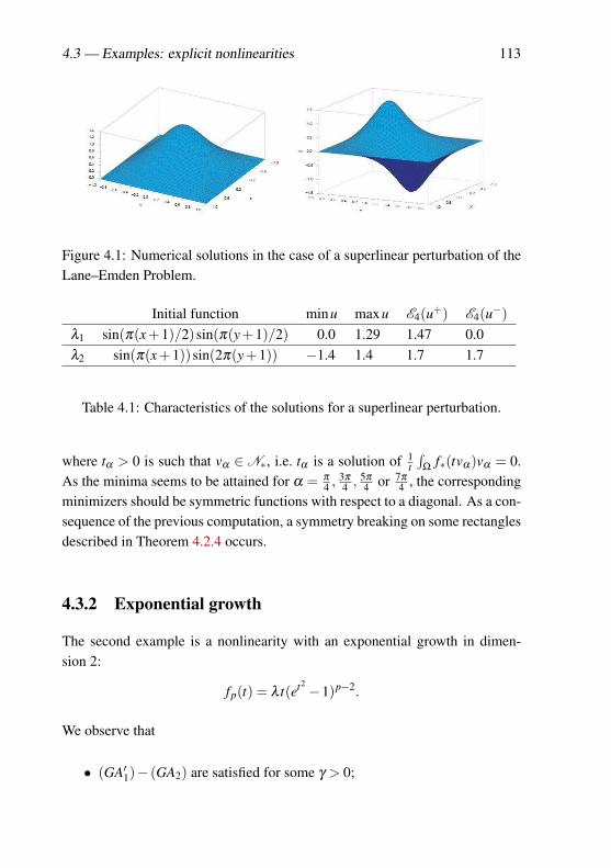
4.3 — Examples: explicit nonlinearities 113
Figure 4.1: Numerical solutions in the case of a superlinear perturbation of theLane–Emden Problem.
Initial function minu maxu E4(u+) E4(u−)λ1 sin(π(x+1)/2)sin(π(y+1)/2) 0.0 1.29 1.47 0.0λ2 sin(π(x+1))sin(2π(y+1)) −1.4 1.4 1.7 1.7
Table 4.1: Characteristics of the solutions for a superlinear perturbation.
where tα > 0 is such that vα ∈N∗, i.e. tα is a solution of 1t∫
Ωf∗(tvα)vα = 0.
As the minima seems to be attained for α = π
4 , 3π
4 , 5π
4 or 7π
4 , the correspondingminimizers should be symmetric functions with respect to a diagonal. As a con-sequence of the previous computation, a symmetry breaking on some rectanglesdescribed in Theorem 4.2.4 occurs.
4.3.2 Exponential growth
The second example is a nonlinearity with an exponential growth in dimen-sion 2:
fp(t) = λ t(et2 −1)p−2.
We observe that
• (GA′1)− (GA2) are satisfied for some γ > 0;
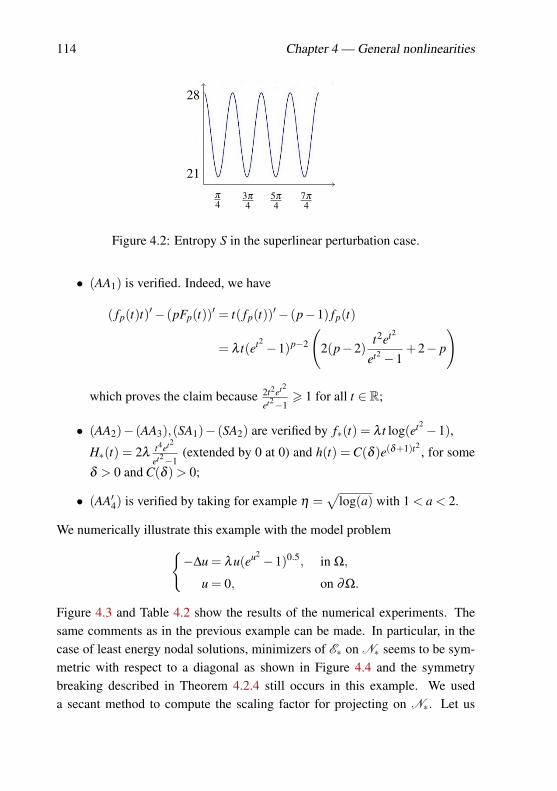
114 Chapter 4 — General nonlinearities
π
43π
45π
47π
4
28
21
Figure 4.2: Entropy S in the superlinear perturbation case.
• (AA1) is verified. Indeed, we have
( fp(t)t)′− (pFp(t))′ = t( fp(t))′− (p−1) fp(t)
= λ t(et2 −1)p−2
(2(p−2)
t2et2
et2 −1+2− p
)
which proves the claim because 2t2et2
et2−1> 1 for all t ∈ R;
• (AA2)− (AA3),(SA1)− (SA2) are verified by f∗(t) = λ t log(et2 −1),
H∗(t) = 2λt4et2
et2−1(extended by 0 at 0) and h(t) = C(δ )e(δ+1)t2
, for some
δ > 0 and C(δ ) > 0;
• (AA′4) is verified by taking for example η =√
log(a) with 1 < a < 2.
We numerically illustrate this example with the model problem−∆u = λu(eu2 −1)0.5, in Ω,
u = 0, on ∂Ω.
Figure 4.3 and Table 4.2 show the results of the numerical experiments. Thesame comments as in the previous example can be made. In particular, in thecase of least energy nodal solutions, minimizers of E∗ on N∗ seems to be sym-metric with respect to a diagonal as shown in Figure 4.4 and the symmetrybreaking described in Theorem 4.2.4 still occurs in this example. We useda secant method to compute the scaling factor for projecting on N∗. Let us
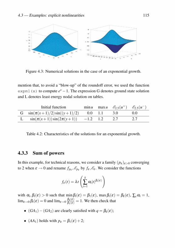
4.3 — Examples: explicit nonlinearities 115
Figure 4.3: Numerical solutions in the case of an exponential growth.
mention that, to avoid a “blow-up” of the roundoff error, we used the functionexpm1(x) to compute ex−1. The expression G denotes ground state solutionand L denotes least energy nodal solution on tables.
Initial function minu maxu E2.5(u+) E2.5(u−)G sin(π(x+1)/2)sin((y+1)/2) 0.0 1.1 3.0 0.0L sin(π(x+1))sin(2π(y+1)) −1.2 1.2 2.7 2.7
Table 4.2: Characteristics of the solutions for an exponential growth.
4.3.3 Sum of powers
In this example, for technical reasons, we consider a family (pε)ε>0 convergingto 2 when ε → 0 and rename fpε
,Epεby fε ,Eε . We consider the functions
fε(t) = λ t
(k
∑i=1
αi|t|βi(ε)
)
with αi,βi(ε) > 0 such that minβi(ε) = β1(ε), maxβi(ε) = βk(ε), ∑i αi = 1,limε→0 βi(ε) = 0 and limε→0
βk(ε)β1(ε) = 1. We then check that
• (GA1)− (GA2) are clearly satisfied with q = βk(ε);
• (AA1) holds with pε = β1(ε)+2;
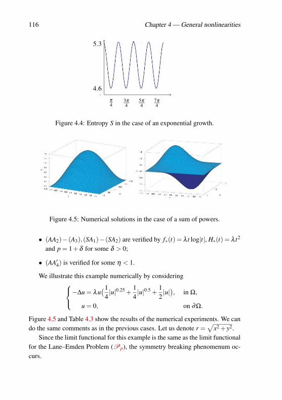
116 Chapter 4 — General nonlinearities
π
43π
45π
47π
4
5.3
4.6
Figure 4.4: Entropy S in the case of an exponential growth.
Figure 4.5: Numerical solutions in the case of a sum of powers.
• (AA2)−(A3),(SA1)−(SA2) are verified by f∗(t) = λ t log|t|, H∗(t) = λ t2
and p = 1+δ for some δ > 0;
• (AA′4) is verified for some η < 1.
We illustrate this example numerically by considering−∆u = λu(1
4|u|0.25 +
14|u|0.5 +
12|u|), in Ω,
u = 0, on ∂Ω.
Figure 4.5 and Table 4.3 show the results of the numerical experiments. We cando the same comments as in the previous cases. Let us denote r =
√x2 + y2.
Since the limit functional for this example is the same as the limit functionalfor the Lane–Emden Problem (Pp), the symmetry breaking phenomenum oc-curs.
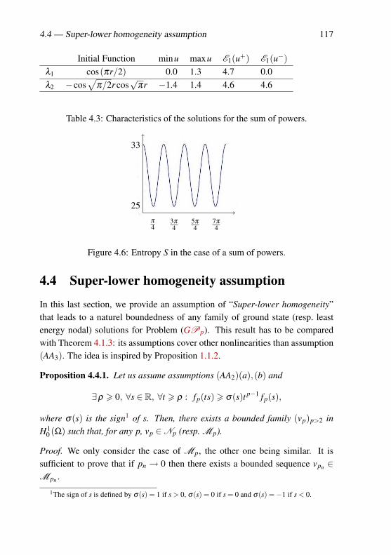
4.4 — Super-lower homogeneity assumption 117
Initial Function minu maxu E1(u+) E1(u−)λ1 cos(πr/2) 0.0 1.3 4.7 0.0λ2 −cos
√π/2r cos
√πr −1.4 1.4 4.6 4.6
Table 4.3: Characteristics of the solutions for the sum of powers.
π
43π
45π
47π
4
33
25
Figure 4.6: Entropy S in the case of a sum of powers.
4.4 Super-lower homogeneity assumption
In this last section, we provide an assumption of “Super-lower homogeneity”that leads to a naturel boundedness of any family of ground state (resp. leastenergy nodal) solutions for Problem (GPp). This result has to be comparedwith Theorem 4.1.3: its assumptions cover other nonlinearities than assumption(AA3). The idea is inspired by Proposition 1.1.2.
Proposition 4.4.1. Let us assume assumptions (AA2)(a),(b) and
∃ρ > 0, ∀s ∈ R, ∀t > ρ : fp(ts)> σ(s)t p−1 fp(s),
where σ(s) is the sign1 of s. Then, there exists a bounded family (vp)p>2 inH1
0 (Ω) such that, for any p, vp ∈Np (resp. Mp).
Proof. We only consider the case of Mp, the other one being similar. It issufficient to prove that if pn → 0 then there exists a bounded sequence vpn ∈Mpn .
1The sign of s is defined by σ(s) = 1 if s > 0, σ(s) = 0 if s = 0 and σ(s) =−1 if s < 0.
118 Chapter 4 — General nonlinearities
Take e2 ∈ E2 and define vp as t+pne+2 + t−pne−2 where t±pn are such that t±pne±2 ∈
Np. Without loss of generality, we can suppose that t±pn are away from 0 (oth-erwise we are done). So, up to a scaling of e2, we can assume that t±pn > ρ forall n. The assumption ensures that
(t±pn)2‖e±2 ‖
2 =∫
Ω
fpn(t±pne±2 )t±pne±2 >
∫Ω
(t±pn)pn fpn(e
±2 )e±2
which implies that
(t±pn)pn−2 6
‖e±2 ‖2∫Ω
fpn(e±2 )e±2
.
As ‖e±2 ‖2 = λ2‖e±2 ‖22 and fpn(e
±2 )→ λe±2 , we just need to study the con-
vergence of the last term in the expression
−log(‖e±2 ‖2)− log(
∫Ω
fpn(e±2 )e±2 )
‖e±2 ‖2−∫
Ωfpn(e
±2 )e±2
·∫
Ω
fpn(e±2 )e±2 −λ2(e±2 )2
pn−2
since the first one converges to −‖e±2 ‖−2, as in Section 1.1. The assumptions(AA2)(a),(b) ensuring that the last term converges to
∫Ω
f∗(e±2 )e±2 , we deducethe boundedness of (t±pn)n∈N and hence of vpn .
Observe now that Proposition 4.4.1 leads in a straightforward way to analternative assumption ensuring the boundedness of ground state (resp. leastenergy nodal) solutions of Problem (GPp). With this alternative, we can treatthe case of the sum of powers without the assumption on βk(ε)β1(ε)−1. If t > 1,we have
λ
n
∑i=1
(αi(ts)βi(ε)ts
)> λ min
i∈1,...,n(tβi(ε)+1)
(n
∑i=1
αisβi(ε)+1
)
= λ t(β1(ε)+1)
(n
∑i=1
αisβi(ε)s
)
and we can conclude recalling that pε = β1(ε) + 2. In fact, we have a bettercontrol on the Nehari manifold. Namely,(
12− 1
β1(ε)+2
)‖u‖2 6 Eε(u)6
(12− 1
βk(ε)+2
)‖u‖2
for every u ∈Nε .
Chapter 5
Lane–Emden problem withNBC
In this chapter, we work with the Lane–Emden Problem with Neumannboundary conditions (NPp)
−∆u+u = λ |u|p−2u, in Ω,
∂ν u = 0, on ∂Ω,(NPp)
where λ > 01. Let us just remark that we work with V ≡ 1 to avoid zero beingthe first eigenvalue of the left-hand side of the equation. So, the operator−∆+Vstays positive definite. In this way, the variational formulation has a mountainpass geometry. The weak solutions of Problem (NPp) are the critical pointsof the energy functional Ep defined on the classical Sobolev space2 H1(Ω) andgiven by
Ep(u) =12
∫Ω
|∇u|2 +u2− λ
p
∫Ω
|u|p.
As for DBC, energy functional Ep is of class C 2(Ω) and satisfies the Palais-Smale condition. Ground state (resp. least energy nodal) solutions exist and
1If Ω is not of class C 1 then the boundary conditions must be perform with the trace operator.2Functions in L2(Ω) with weak derivative belonging to L2(Ω), with associated norm ‖u‖2 =∫
Ω|∇u|2 +u2.
119
120 Chapter 5 — Lane–Emden problem with NBC
are minima of the energy functional Ep on the Nehari manifold Np (resp. nodalNehari set Mp) defined by
Np := u ∈H1(Ω)\0 : 〈dEp(u),u〉= 0, Mp := u ∈H1(Ω) : u± ∈Np,
where〈dEp(u),v〉=
∫Ω
∇u∇v+uv−λ
∫Ω
|u|p−2uv.
We have that a ground state solution (resp. l.e.n.s) must not change sign (resp.possess two nodal domains). These facts can be proven using the same argu-ments as for the DBC (see Introduction of Chapter 1). For any u ∈ H1(Ω),u ∈Np if and only if ∫
Ω
|∇u|2 +u2 = λ2
∫Ω
|u|p, (5.1)
which implies that( 1
2−1p
)‖u‖2 = Ep(u). We also have that, for any u∈H1(Ω)\
0, there exists one and only one positive multiplicative factor t∗ > 0 such thatt∗u ∈ Np. As zero is a strict local minimum of Ep, it implies that Ep(t∗u) =maxt>0(Ep(tu)). If u ∈ H1(Ω), u+ 6= 0 and u− 6= 0, then u ∈Mp if and only if∫
Ω
|∇u+|2 +(u+)2 = λ
∫Ω
|u+|p and∫
Ω
|∇u−|2 +(u−)2 = λ
∫Ω
|u−|p. (5.2)
At u ∈ H1(Ω) \ 0, we can project it on Mp by maximizing the energy func-tional on the quarter of plane defined by u+ and u−.
To start, in Section 5.1, we show that techniques and results developed inChapter 1 are also working for Neumann boundary conditions. Let us de-note λi (resp. Ei) the eigenvalues without multiplicity (resp. eigenspaces) of−∆ + id with NBC. By homogeneity, without loss of generality, we can assumethat λ = λ1 (resp. λ2) when we are working with ground state solutions (resp.l.e.n.s.). In particular, we obtain that ground state solutions must respect thesymmetries of Ω for p close to 2. It is an alternative to the Gidas, Ni andNirenberg method which is only applicable for DBC. Moreover, ground statesolutions must be the non-zero constant solutions for p close to 2. In fact, weshow the uniqueness of the positive solution for p close to 2. Concerning leastenergy nodal solutions, we obtain similar symmetries as for DBC when Ω is arectangle, a radial domain or a square. We also obtain some symmetry breakingon some rectangles.
121
Then, in Section 5.2, we focus on larger p and ground state solutions. Westudy for which p we obtain the first symmetry breaking whose the existence isimplied by the results in [62] (see Introduction page 25), i.e. we are looking forthe first p where ground state solutions are not a constant function anymore.For this, in Section 5.2.1, we need to work with the notion of Morse index of Ep
at the non-zero constant solutions. For a critical point u of an application F,the Morse index is defined as
indM(u,F) := supdimE : dimE < +∞,〈d2F(u),v,v〉< 0 if v ∈ E \0.
It corresponds to the number of independent descent directions of the secondderivative. As a ground state solution u minimizes the energy functional onNp, a manifold of co-dimension 1 composed of local maxima, we have thatindM(u,Ep) = 1. The descent direction is given by u itself. As consequence, weprove that non-zero constant solutions cannot be ground state solutions any-more for p > 1+λ2. To know whether 1+λ2 is optimal, we analyze bifurcationsstarting from the non-zero constant solutions in Section 5.2.2. In particular, weobtain bifurcations when p is equal to 1 + λi. For this part, we use the fol-lowing traditional Krasnoselskii-Boehme-Marino theorem. To understand wellwhat we mean by bifurcation, let us consider a continuous function
F : R×H→ H : (t,u) 7→ F(t,u),
where H is a Banach space. Assume that there exists v ∈ H such that, for anyt ∈ R, F(t,v) = 0. In this context, let us define notions of bifurcation:
• (λ ,v) ∈ R×H is a bifurcation point for the equation F(t,u) = 0 if andonly if there exists a sequence (λn,vn)→ (λ ,v), vn 6= v, such that, for anyn ∈ N, F(λn,vn) = 0.
In this case, sequence (vn)n∈N is called bifurcation sequence.
• (λ ,v)∈R×H is a continuous bifurcation point for F(t,u) = 0 if and onlyif there exists a non-trivial continuum3 of solutions for equation F(t,u) =0 containing (λ ,v).
3Connected domain.
122 Chapter 5 — Lane–Emden problem with NBC
In this last case, the branch is called bifurcation branch. If it is “maxi-mal”4, the branch (resp. point) is called global bifurcation branch (resp.global bifurcation point).
Krasnoselskii-Boehme-Marino Theorem.Let F : I×H→H : (t,u) 7→ F(t,u) be a continuous function, where I ⊆R is aninterval and H is a Banach space, such that F(λ ,0) = 0 for any λ ∈ I.
• If F is of class C 1 in a neighbourhood of (λ ,0) and (λ ,0) is a bifurcationpoint of F then F ′u(λ ,0) is not invertible.
• Let assume that for each (λ ,u) ∈ I×H,
F(λ ,u) = L(λ ,u)−N(λ ,u), L(λ , ·) = λ id−T and N(λ ,u) = o(‖u‖),(5.3)
with T linear, T and N completely continuous, and the last equality beinguniform on each compact set of λ .
If λ∗ is an eigenvalue of T with odd multiplicity, then (λ∗,0) is a globalbifurcation point for F(t,u) = 0.
• Let assume that H is a Hilbert space and that for each (λ ,u) ∈ I×R,F(λ ,u) = ∇uh(λ ,u) where
h(λ ,u) = 〈L(λ ,u),u〉/2−g(λ ,u), L(λ , ·) = λ id−T,
and ∇g(λ ,u) = o(‖u‖),(5.4)
with T linear and symmetric, g(λ , ·) ∈ C 2 for all λ , and the last equalitybeing uniform on each compact set of λ .
If λ∗ is an eigenvalue of T with finite multiplicity and h(λ , ·) verifies thePalais-Smale condition for each λ , then (λ∗,0) is a bifurcation point forF(t,u) = 0.
The first point is the contraposition of the implicit function theorem (see page34). The second point, proved by Krasnoselskii, is based on the degree theoryand the third one follows from the Morse theory (see e.g. [21, 50]).
4The branch cannot be extended. Let us remark that each bifurcation branch can be extended toa “maximal” branch.
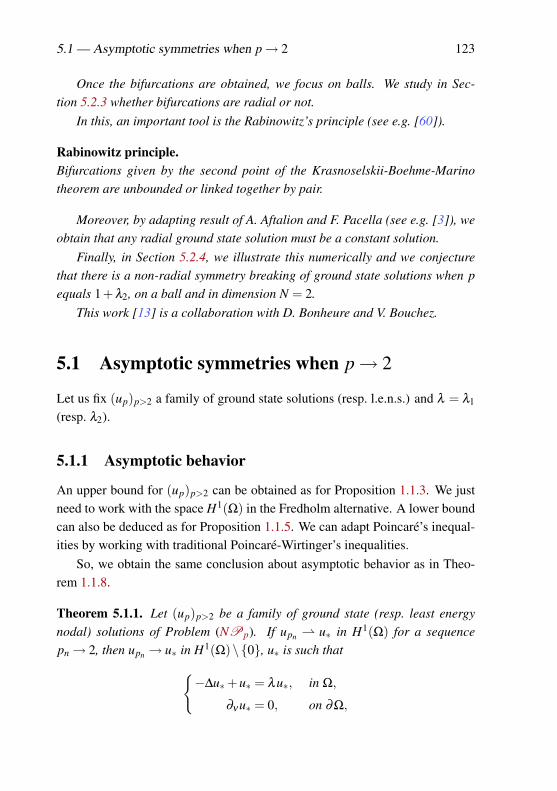
5.1 — Asymptotic symmetries when p→ 2 123
Once the bifurcations are obtained, we focus on balls. We study in Sec-tion 5.2.3 whether bifurcations are radial or not.
In this, an important tool is the Rabinowitz’s principle (see e.g. [60]).
Rabinowitz principle.Bifurcations given by the second point of the Krasnoselskii-Boehme-Marinotheorem are unbounded or linked together by pair.
Moreover, by adapting result of A. Aftalion and F. Pacella (see e.g. [3]), weobtain that any radial ground state solution must be a constant solution.
Finally, in Section 5.2.4, we illustrate this numerically and we conjecturethat there is a non-radial symmetry breaking of ground state solutions when pequals 1+λ2, on a ball and in dimension N = 2.
This work [13] is a collaboration with D. Bonheure and V. Bouchez.
5.1 Asymptotic symmetries when p→ 2
Let us fix (up)p>2 a family of ground state solutions (resp. l.e.n.s.) and λ = λ1
(resp. λ2).
5.1.1 Asymptotic behavior
An upper bound for (up)p>2 can be obtained as for Proposition 1.1.3. We justneed to work with the space H1(Ω) in the Fredholm alternative. A lower boundcan also be deduced as for Proposition 1.1.5. We can adapt Poincaré’s inequal-ities by working with traditional Poincaré-Wirtinger’s inequalities.
So, we obtain the same conclusion about asymptotic behavior as in Theo-rem 1.1.8.
Theorem 5.1.1. Let (up)p>2 be a family of ground state (resp. least energynodal) solutions of Problem (NPp). If upn u∗ in H1(Ω) for a sequencepn→ 2, then upn → u∗ in H1(Ω)\0, u∗ is such that
−∆u∗+u∗ = λu∗, in Ω,
∂ν u∗ = 0, on ∂Ω,
124 Chapter 5 — Lane–Emden problem with NBC
with λ = λ1 (resp. λ2), and
E∗(u∗) = infE∗(u) : u ∈ E \0 and 〈dE∗(u),u〉= 0,
with E = E1 (resp. E2), the first (resp. second) eigenspace of −∆+ id.
5.1.2 Symmetries
For this part, we are directly working in the same way as the “general technique”described in Section 1.4. To obtain the uniqueness result 1.4.1, we just need aspreviously to adapt Poincaré’s inequality. Clearly, after this, Proposition 1.4.2only depends on the nonlinearity.
Theorem 5.1.2. Let (Gα)α∈E with E = E1 (resp. E = E2) be groups acting onH1(Ω) in such a way that, for every g ∈ Gα and for every u ∈ H1(Ω),
g(E) = E, g(E⊥) = E⊥, gα = α and Ep(gu) = Ep(u).
Then, for all M > 0, if p is close enough to 2, any ground state (resp. leastenergy nodal) solution up ∈ u∈B(0,M) : PE(u) /∈B(0, 1
M ) of Problem (NPp)belongs to the invariant set of Gαp where αp := PEup.
We can obtain a little bit more. We show that ground state solution is con-stant for p close to 2, at least on regular domains.
Theorem 5.1.3. If Ω is of class C 2 or a product of intervals, there exists p > 2
such that if 2 < p 6 p, then the non-zero constant solutions ±( 1
λ
) 1p−2 are the
unique ground state solutions of Problem (NPp).
Proof. Let us consider a family of positive ground state solutions (up)p>2.Ideas are similar for negative solutions. By homogeneity, we can w.l.o.g. as-sume that λ = λ1. Let us denote by vp and wp the projections of up respectivelyon E1 and E⊥1 . By using the spectral theory, the fact that, as E1 is the set of
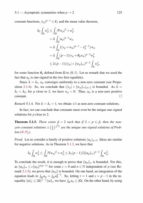
5.1 — Asymptotic symmetries when p→ 2 125
constant functions, |vp|p−1 ∈ E1 and the mean value theorem,
λ2
∫Ω
w2p ≤
∫Ω
|∇wp|2 +w2p
= λ
∫Ω
|up|p−1wp
= λ
∫Ω
((vp +wp)p−1− vp−1
p)
wp
= λ
∫Ω
(p−1)(vp +θpwp)p−2w2p
≤ λ (p−1)(|vp|+‖wp‖∞)p−2∫
Ω
w2p,
for some function θp defined from Ω to (0,1). Let us remark that we used thefact that up is one-signed in the two first equalities.
Since λ = λ1, up converges uniformly to a non-zero constant (see Propo-sition 2.1.4). So, we conclude that (|vp|+ ‖wp‖∞)p>2 is bounded. As λ =λ1 < λ2, for p close to 2, we have wp = 0. Thus, up is a non-zero positiveconstant.
Remark 5.1.4. For λ = λ1 = 1, we obtain ±1 as non-zero constant solutions.
In fact, we can conclude that constants must even be the unique one-signedsolutions for p close to 2.
Theorem 5.1.5. There exists p > 2 such that if 2 < p 6 p, then the non-
zero constant solutions ±( 1
λ
) 1p−2 are the unique one-signed solutions of Prob-
lem (NPp).
Proof. Let us consider a family of positive solutions (up)p>2. Ideas are similarfor negative solutions. As in Theorem 5.1.3, we have that
λ2
∫Ω
w2p ≤
∫Ω
|∇wp|2 +w2p ≤ λ1(p−1)(2‖up‖∞)p−2
∫Ω
w2p.
To conclude the result, it is enough to prove that ‖up‖∞ is bounded. For this,as ‖up‖∞ ≤ c‖up‖n(p−1) for some c > 0 and n ∈ N independent of p (see Re-mark 2.1.5), we prove that ‖up‖ is bounded. On one hand, an integration of theequation leads to
∫Ω
up =∫
Ωup−1
p . So, letting r = 1 and s = p− 1 in the in-equality ‖u‖r ≤ |Ω|
1r−
1s ‖u‖s, we have
∫Ω
up ≤ |Ω|. On the other hand, by using
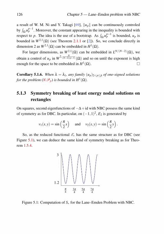
126 Chapter 5 — Lane–Emden problem with NBC
a result of W. M. Ni and Y. Takagi [69], ‖up‖ can be continuously controledby∫
Ωup−1
p . Moreover, the constant appearing in the inequality is bounded withrespect to p. The idea is the use of a bootstrap. As
∫Ω
up−1p is bounded, up is
bounded in W 2,1(Ω) (see Theorem 2.1.1 or [2]). So, we conclude directly indimension 2 as W 2,1(Ω) can be embedded in H1(Ω).
For larger dimensions, as W 2,1(Ω) can be embedded in LN/(N−2)(Ω), we
obtain a control of up in W 2, N(N−2)(p−1) (Ω) and so on until the exponent is high
enough for the space to be embedded in H1(Ω).
Corollary 5.1.6. When λ = λ1, any family (up)2<p≤p of one-signed solutionsfor the problem (NPp) is bounded in H1(Ω).
5.1.3 Symmetry breaking of least energy nodal solutions onrectangles
On squares, second eigenfunctions of−∆+ id with NBC possess the same kindof symmetry as for DBC. In particular, on (−1,1)2, E2 is generated by
v1(x,y) = sin(
π
2x)
and v2(x,y) = sin(
π
2y)
.
So, as the reduced functional E∗ has the same structure as for DBC (seeFigure 5.1), we can deduce the same kind of symmetry breaking as for Theo-rem 1.5.4.
π
43π
45π
47π
4
3
1.2
Figure 5.1: Computation of S∗ for the Lane–Emden Problem with NBC.
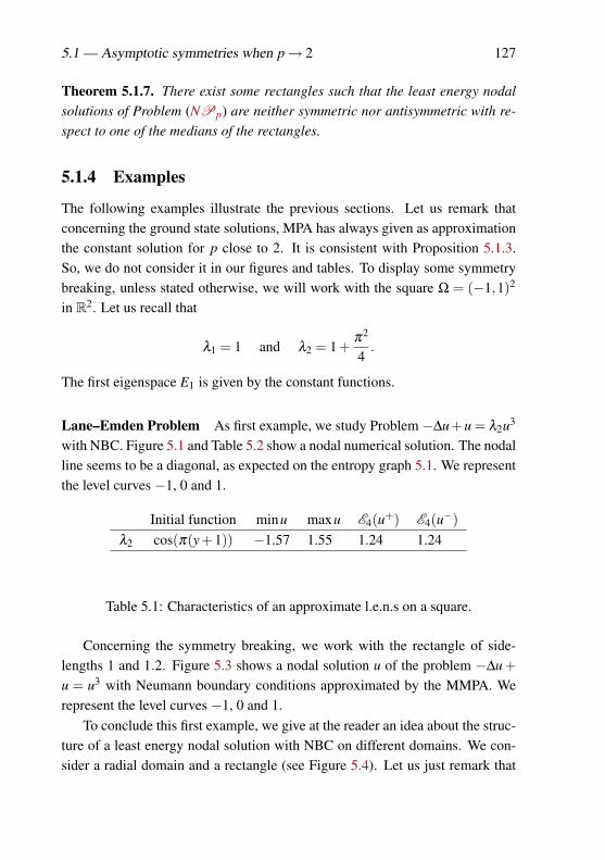
5.1 — Asymptotic symmetries when p→ 2 127
Theorem 5.1.7. There exist some rectangles such that the least energy nodalsolutions of Problem (NPp) are neither symmetric nor antisymmetric with re-spect to one of the medians of the rectangles.
5.1.4 Examples
The following examples illustrate the previous sections. Let us remark thatconcerning the ground state solutions, MPA has always given as approximationthe constant solution for p close to 2. It is consistent with Proposition 5.1.3.So, we do not consider it in our figures and tables. To display some symmetrybreaking, unless stated otherwise, we will work with the square Ω = (−1,1)2
in R2. Let us recall that
λ1 = 1 and λ2 = 1+π2
4.
The first eigenspace E1 is given by the constant functions.
Lane–Emden Problem As first example, we study Problem −∆u+u = λ2u3
with NBC. Figure 5.1 and Table 5.2 show a nodal numerical solution. The nodalline seems to be a diagonal, as expected on the entropy graph 5.1. We representthe level curves −1, 0 and 1.
Initial function minu maxu E4(u+) E4(u−)λ2 cos(π(y+1)) −1.57 1.55 1.24 1.24
Table 5.1: Characteristics of an approximate l.e.n.s on a square.
Concerning the symmetry breaking, we work with the rectangle of side-lengths 1 and 1.2. Figure 5.3 shows a nodal solution u of the problem −∆u +u = u3 with Neumann boundary conditions approximated by the MMPA. Werepresent the level curves −1, 0 and 1.
To conclude this first example, we give at the reader an idea about the struc-ture of a least energy nodal solution with NBC on different domains. We con-sider a radial domain and a rectangle (see Figure 5.4). Let us just remark that
128 Chapter 5 — Lane–Emden problem with NBC
−2.0
−1.5
−1.0
−0.5
0.0
0.5
1.0
1.5
2.0
Z
−1.0 −0.8 −0.6 −0.4 −0.2 0.0 0.2 0.4 0.6 0.8 1.0
Y
−1
0
1X
Figure 5.2: Numerical solutions of the Lane–Emden Problem with NBC.
Initial function minu maxu E4(u+) E4(u−)cos(π x
2 ) −4.6 6.8 8.2 3.2
Table 5.2: Characteristics of a l.e.n.s. on (0,1)× (0,1.2).
the same structure will take place in the following examples. In particular, onthe rectangle, the solution seems only to have one dimension of variation.
In previous sections, to simplify technical issues, we focused on a power asnonlinearity. However, we can clearly mix the results of Chapter 4 and this one.In this way, we obtain that asymptotic and symmetry results are still valid formore general nonlinearities fp (satisfying the assumptions of Chapter 4). Wejust need to be careful with Proposition 5.1.3. To obtain the result, we must beable to control fp(vp +wp)− fp(vp) to apply the mean value theorem.
Superlinear perturbation of Lane–Emden Problem Let us consider the fol-lowing problem
−∆u+u = λ2u3 +2u5, in Ω,
∂ν u = 0, on ∂Ω.(5.5)
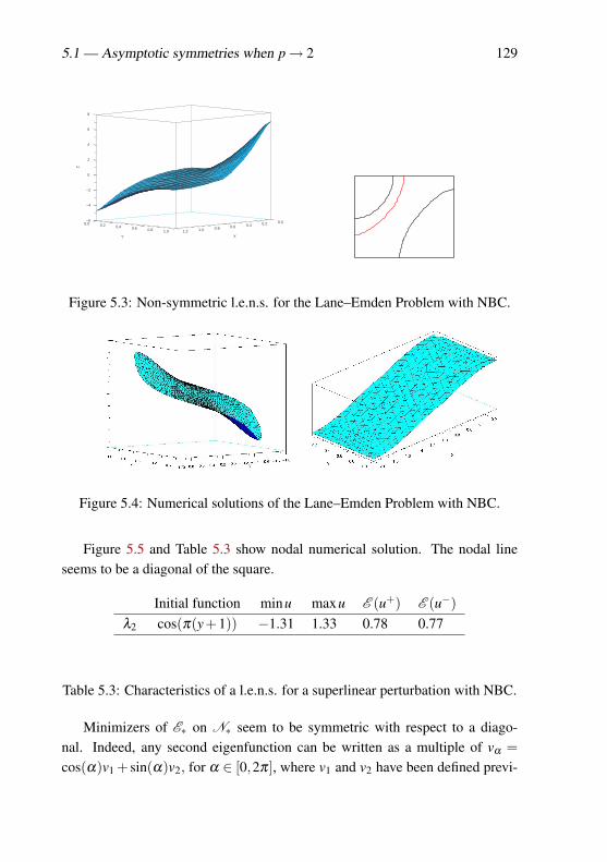
5.1 — Asymptotic symmetries when p→ 2 129
−6
−4
−2
0
2
4
6
8
Z
0.00.20.40.60.81.01.2X
0.0 0.2 0.4 0.6 0.8 1.0Y
Figure 5.3: Non-symmetric l.e.n.s. for the Lane–Emden Problem with NBC.
Figure 5.4: Numerical solutions of the Lane–Emden Problem with NBC.
Figure 5.5 and Table 5.3 show nodal numerical solution. The nodal lineseems to be a diagonal of the square.
Initial function minu maxu E (u+) E (u−)λ2 cos(π(y+1)) −1.31 1.33 0.78 0.77
Table 5.3: Characteristics of a l.e.n.s. for a superlinear perturbation with NBC.
Minimizers of E∗ on N∗ seem to be symmetric with respect to a diago-nal. Indeed, any second eigenfunction can be written as a multiple of vα =cos(α)v1 + sin(α)v2, for α ∈ [0,2π], where v1 and v2 have been defined previ-
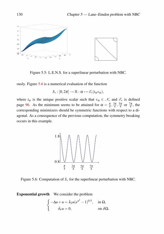
130 Chapter 5 — Lane–Emden problem with NBC
Figure 5.5: L.E.N.S. for a superlinear perturbation with NBC.
ously. Figure 5.6 is a numerical evaluation of the function
S∗ : [0,2π]→ R : α 7→ E∗(tα vα),
where tα is the unique positive scalar such that vα ∈ N∗ and E∗ is definedpage 96. As the minimum seems to be attained for α = π
4 , 3π
4 , 5π
4 or 7π
4 , thecorresponding minimizers should be symmetric functions with respect to a di-agonal. As a consequence of the previous computation, the symmetry breakingoccurs in this example.
π
43π
45π
47π
4
1.8
0.8
Figure 5.6: Computation of S∗ for the superlinear perturbation with NBC.
Exponential growth We consider the problem−∆u+u = λ2u(eu2 −1)0.5, in Ω,
∂ν u = 0, on ∂Ω.
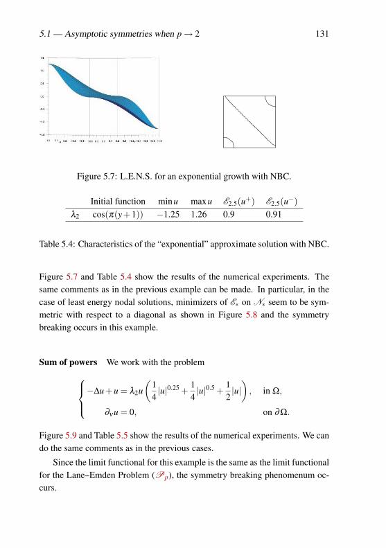
5.1 — Asymptotic symmetries when p→ 2 131
Figure 5.7: L.E.N.S. for an exponential growth with NBC.
Initial function minu maxu E2.5(u+) E2.5(u−)λ2 cos(π(y+1)) −1.25 1.26 0.9 0.91
Table 5.4: Characteristics of the “exponential” approximate solution with NBC.
Figure 5.7 and Table 5.4 show the results of the numerical experiments. Thesame comments as in the previous example can be made. In particular, in thecase of least energy nodal solutions, minimizers of E∗ on N∗ seem to be sym-metric with respect to a diagonal as shown in Figure 5.8 and the symmetrybreaking occurs in this example.
Sum of powers We work with the problem−∆u+u = λ2u(
14|u|0.25 +
14|u|0.5 +
12|u|)
, in Ω,
∂ν u = 0, on ∂Ω.
Figure 5.9 and Table 5.5 show the results of the numerical experiments. We cando the same comments as in the previous cases.
Since the limit functional for this example is the same as the limit functionalfor the Lane–Emden Problem (Pp), the symmetry breaking phenomenum oc-curs.
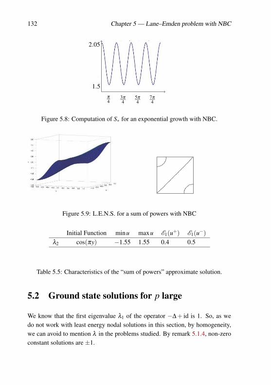
132 Chapter 5 — Lane–Emden problem with NBC
π
43π
45π
47π
4
2.05
1.5
Figure 5.8: Computation of S∗ for an exponential growth with NBC.
Figure 5.9: L.E.N.S. for a sum of powers with NBC
Initial Function minu maxu E1(u+) E1(u−)λ2 cos(πy) −1.55 1.55 0.4 0.5
Table 5.5: Characteristics of the “sum of powers” approximate solution.
5.2 Ground state solutions for p large
We know that the first eigenvalue λ1 of the operator −∆ + id is 1. So, as wedo not work with least energy nodal solutions in this section, by homogeneity,we can avoid to mention λ in the problems studied. By remark 5.1.4, non-zeroconstant solutions are ±1.
5.2 — Symmetries for large p 133
5.2.1 The ground state solutions are not radial for p large
As mentioned in the Introduction, we expect a symmetry breaking. To know forwhich p a ground state solution of Problem (NPp) is not ±1 anymore, we willuse Morse index of Ep at ±1. Let us consider the linearized problem of (NPp)around u ∈ H1(Ω),
−∆h+h− (p−1)|u|p−2h = µh, in Ω,
∂ν h = 0, on ∂Ω.(NP ′
p)
Proposition 5.2.1. For any i ∈N\0, if λi < p−1≤ λi+1 then indM(±1,Ep)equals ∑k≤i dimEk.
Proof. By definition, the Morse index of Ep at a critical point u corresponds tothe sum of the dimensions of the eigenspaces associated to the negative eigen-values µ of the Problem (NP ′
p).Let us consider u = 1 or −1. The solutions h of Problem (NP ′
p) are eigen-functions of −∆ + id associated to the eigenvalue p− 1 + µ . We obtain thatµi = λi− (p−1), which concludes the proof.
As a ground state solution has a Morse index equals to 1, we obtain thefollowing corollary.
Corollary 5.2.2. Function 1 (resp. −1) cannot be a ground state solution if
p−1 > λ2.
5.2.2 Bifurcation results
In this section, we try to obtain some bifurcations of solutions starting from±1.By using previous Krasnoselskii-Boehme-Marino bifurcation result (see page120), we obtain that the first bifurcation point (p,±1) occurs for p = 1+λ2.
Theorem 5.2.3. For 2 < p < 2∗, (p,±1) is a bifurcation point for the prob-lem (NPp) if and only if p = 1+λi, for i > 1.
Proof. We prove it for 1. The idea is similar for−1. First, we rephrase our Pro-blem (NPp). The fact that (p,u) is a solution of Problem (NPp) is equivalentto the fact that (p−1,u−1) = (q,v) solves L∗(q,v)−N∗(q,v) = 0 where
134 Chapter 5 — Lane–Emden problem with NBC
L∗ : (1,2∗−1)×H1→ (H1)′ : (q,v) 7→ (−∆+ id)v−qv,N∗ : (1,2∗−1)×H1→ (H1)′ : (q,v) 7→ |1+ v|q−1(1+ v)−qv−1.
For technical reasons, we work with equation q−1(L∗−N∗) = 0. We usethe third part of the Krasnoselskii-Boehme-Marino result. Composing withthe canonical isomorphism between H1(Ω) and (H1(Ω))′, q−1L∗(q,v) equalsq−1v− (−∆ + id)−1v in H1(Ω). This plays the role of operator L in equa-tion (5.4). It is enough to prove that limv→0
N∗(q,v)‖v‖ = 0 uniformly on compact
sets of q in (1,2∗− 1). It will be established if we show that if (vn)n∈N is asequence in H1(Ω) with norm equals to 1, (tn)n∈N converging to 0 and (qn)n∈Nbounded by q, then, up to a subsequence, limn→∞
N∗(qn,tnvn)tn
= 0. We show that
limn→∞
1tn
∫Ω
(|1+ tnvn|qn−1(1+ tnvn)−1−qntnvn
)w = 0,
uniformly with respect to w ∈ H1(Ω) with ‖w‖ = 1. We have, for any n ∈ N,because qn+1
qnand qn +1 are less than 2∗,
1tn
∫Ω
(|1+ tnvn|qn−1(1+ tnvn)−1−qntnvn
)w
≤ 1tn
∥∥|1+ tnvn|qn−1(1+ tnvn)−1−qntnvn∥∥ qn+1
qn‖w‖qn+1.
By using the mean value theorem, there exists θn ∈ (0,1) such that
1tn
(|1+ tnvn|qn−1(1+ tnvn)−1−qntnvn
)= qn|1+θntnvn|qn−1vn−qnvn→ 0
almost everywhere and, as we can assume that 0≤ tn ≤ 1 w.l.o.g.,∣∣∣∣ 1tn
(∣∣1+ tnvn∣∣qn−1(1+ tnvn)−1−qntnvn
)∣∣∣∣≤ 2qn∣∣1+ |vn|
∣∣q ≤ 2q∣∣1+ |vn|
∣∣q.(5.6)
Using Lebesgue’s dominated convergence theorem, we infer the expected re-sult.
Thus, as the Problem (NPp) respects the Palais-Smale condition, we canapply the third point of the Krasnoselskii-Boehme-Marino result (see page 120)to conclude the existence of bifurcation branches starting from 0 when q equalsλi. So, our Problem (NPp) has bifurcations starting from 1 when p equals1+λi, for some i.
5.2 — Symmetries for large p 135
If p− 1 6= λi, we obtain that there does not exist bifurcations. Indeed, theoperator ∂v(L∗−N∗)(p−1,0) is invertible. We conclude by the implicit func-tion theorem (see page 34).
Remark 5.2.4. • Using the same arguments, we can conclude from the sec-ond statement of the Krasnoselskii-Boehme-Marino result (see page 120)that if λi has odd multiplicity then we obtain global bifurcations.
• By Rabinowitz’s principle (see page 121), we obtain that bifurcationbranches are unbounded or linked together by pair when the multiplic-ity of λi is odd.
• In dimension N = 2, as 2∗ = +∞, we have infinitely many bifurcations.
5.2.3 Specific case: a ball
In this section, we focus on the ball B(0,1). We already know that a ground statesolution cannot be a constant function for p > 1+λ2 (see Corollary 5.2.2). Wewould like to know whether they stay radial functions.
Non-radial solution We start by adapting to the Neumann boundary case,results of A. Aftalion and F. Pacella (see [3]). They proved, for the Lane-EmdenProblem with Dirichlet boundary conditions, that nodal radial solutions has aMorse index at least equals to N +1.
Lemma 5.2.5. Let Lv := −∆v + v− (p− 1)|up|p−2v, up a solution of Prob-lem (NPp). Let us denote, for any i ∈ 1,2, . . . ,N,
Ωi = x = (x1, . . . ,xN) ∈ B(0,1) : xi = 0,
Ω+i = x = (x1, . . . ,xN) ∈ B(0,1) : xi > 0
andΩ−i = x = (x1, . . . ,xN) ∈ B(0,1) : xi < 0.
Let µi denote the first eigenvalue of L in Ω+i with Dirichlet boundary condi-
tions on Ωi and Neumann boundary conditions on ∂Ω+i \Ωi; and ψi the first
eigenfunction related to µi. If up is even with respect to xi, let us denote ψ∗i the
136 Chapter 5 — Lane–Emden problem with NBC
extension of ψi on all B(0,1) such that ψ∗i is odd with respect to xi. Then, ψ∗i isnot a first eigenfunction of L in B(0,1) with Neumann boundary conditions.
Moreover, if up is even with respect to the variables x1, . . . ,xk, 1 ≤ k ≤ N,ψ∗1 , . . . ,ψ∗k constructed are independent and give k eigenfunctions of L (none ofwhich is a first eigenfunction).
Proof. As the potential 1− (p−1)|up|p−2 is bounded, the first eigenvalue of Lis real and the unique first eigenfunction is a one-signed function (see e.g. [34]).We clearly have L(ψ∗i ) = µiψ
∗i on B(0,1) \Ωi and ψ∗i satisfies the Neumann
boundary conditions on ∂B(0,1). It remains to verify that L(ψ∗i ) = µiψ∗i on Ωi.
As ψ∗i = 0 on Ωi, we have
∀ j 6= i, ∂x j ψ∗i = ∂
2x j
ψ∗i = 0.
As ψi is an eigenfunction of L, by a continuous extension of ∂ 2xi
ψi on Ωi and asψ∗i is odd, we have
−N
∑j=0
∂2x j
ψ +0− (p−1)|up|p−20 = 0
and thus ∂ 2xi
ψ∗i = 0 on Ωi. So, L(ψ∗i ) = µiψ∗i on Ωi. As ψ∗i is a sign-changing
function, it is not a first eigenfuntion. It concludes the first part of the proof.The independence of ψ∗i , for i ∈ 1, . . . ,k, is easily established using the
fact that ψ∗i is the only function which is not equal to zero in the direction ofxi.
Proposition 5.2.6. If up is a non-constant one-signed radial solution, its Morseindex is at least N +1.
Proof. Without loss of generality, we can assume that up ≥ 0 on B(0,1). ByLemma 5.2.5, we have the existence of N independent eigenfunctions ψ∗i (noneof which is a first eigenfunction), for i ∈ 1, . . . ,N, of Lv := −∆v + v− (p−1)|u|p−1v with Neumann boundary conditions. Since the corresponding eigen-values of ψ∗i are above the first one, it is sufficient to prove that eigenvaluesrelated to ψ∗i are negative.
Let i ∈ 1, . . . ,N. We have ∂xiup = 0 on Ωi (because up is radial) andon ∂B(0,1) (because up is constant on the boundary and satisfies the Neumann
5.2 — Symmetries for large p 137
boundary conditions). Pick x∈Ω+i such that ∂xiup(x) 6= 0 (such x exists because
up is radially symmetric and not constant). Let D be the connected componentof x|∂xiup(x) 6= 0 containing x.
Differentiation of the equation (NPp) for which up is a solution gives
L(∂xiup) =−∆(∂xiup)+∂xiup− (p−1)|up|p−2∂xiu = 0.
Since ∂xiup does not change sign on D, 0 is the first eigenvalue of L in D withDirichlet boundary conditions. As D⊆ Ω
+i , the first eigenvalue of L in Ω
+i for
Dirichlet boundary conditions is non-positive. By applying the Höpf’s Lemma(see 2.2.1), we know that first eigenvalue for mixed boundary conditions isstrictly lower than first eigenvalue for Dirichlet boundary conditions. So, wehave that the first eigenvalue of L in Ω
+i for Dirichlet boundary conditions on
Ωi and Neumann on ∂B(0,1)\Ωi is negative, which concludes the proof.
As the Morse index of ground state solutions is 1, the previous result impliesthe following theorem.
Theorem 5.2.7. If up is a radially symmetric ground state solution, then up isconstant.
Study of eigenspaces Existence of radial bifurcations proved in the followingwill be related to eigenvalues λi and eigenspaces Ei of −∆ + id in H1(B(0,1))with Neumann boundary conditions. Let us explain here the structure of thesefunctions. The technique is the same as for Dirichlet boundary conditions (seeSection 1.3 in Chapter 1). The first eigenvalue λ1 equals 1 and first eigen-functions are the constant functions. By the separation of variable r = |x| andσ = x
|x| , for each i > 1, there exists an unique (k,q) ∈N×N\0 such that, forall eigenfunction u associated to λi,
λi = j2µk,q +1 with jµk,q the qst positive critical point of the Bessel function Jµk ,
where µk =(k + N−2
2
). We have that
u(x) = Jµk( jµk,qr)r2−N
2 Pk
(x|x|
)with
Pk : RN → R an harmonic homogenous polynomial of degree k.
138 Chapter 5 — Lane–Emden problem with NBC
Let us remark that radial eigenfunctions are given when k = 0, i.e. whenwe consider critical points of the Bessel function JN−2
2. For each eigenspace
Ei, the dimension of the intersection with radial functions is 0 or 1. Moreover,for functions in Ei with k = 0, the radial part is given by Jµ0( jµ0,qr)r
2−N2 . We
remark that intersections of those functions with 0 are simple.
Radial bifurcation We would like to know whether solutions along the bi-furcations given in Proposition 5.2.3 belong to H1
rad(B(0,1)), the subspace ofradially symmetric functions of H1(B(0,1)). In particular, we obtain that bifur-cation branches at (1+λ2,±1) are not radial.
Theorem 5.2.8. • If Ei ∩H1rad(B(0,1)) = 0, (1 + λi,±1) is not a radial
bifurcation point in H1rad(B(0,1)).
• If Ei ∩H1rad(B(0,1)) 6= 0, (1 + λi,±1) is a radial bifurcation point in
H1rad(B(0,1)).
Proof. We consider the operator L∗−N∗ defined in the proof of Theorem 5.2.3restricted to H1
rad(B(0,1)). If the eigenspace Ei of −∆ + id does not containnon-trivial radial functions, the operator
∂u(L∗−N∗)|H1rad
(λi,0)
is invertible. Indeed, the operator is a Fredholm operator of index 0 and ∂u(L∗−N∗)|H1
rad(λi,0)w = 0 if and only if
w ∈ Ei∩H1rad(B(0,1)).
So, by the first point of the Krasnoselskii-Boehme-Marino result (see page 120),(λi,0) is not a bifurcation point for (L∗−N∗)|H1
rad.
Now, if Ei ∩H1rad(B(0,1)) 6= 0, we can follow the same arguments as in
the proof of Theorem 5.2.3 in the space H1rad to establish the existence of a radial
bifurcation point.
Remark 5.2.9. Let us consider the ball of radius R. When R→ +∞, we obtainthat eigenvalues λi of −∆ + id go to 1. So, at 2 < p < 2∗ fixed, for any n > 0,there exists Rn > 1 such that, on the ball BRn , we have at least n radial globalbifurcations.
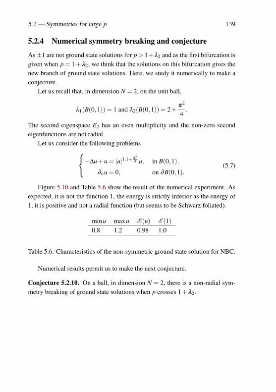
5.2 — Symmetries for large p 139
5.2.4 Numerical symmetry breaking and conjecture
As±1 are not ground state solutions for p > 1+λ2 and as the first bifurcation isgiven when p = 1+λ2, we think that the solutions on this bifurcation gives thenew branch of ground state solutions. Here, we study it numerically to make aconjecture.
Let us recall that, in dimension N = 2, on the unit ball,
λ1(B(0,1)) = 1 and λ2(B(0,1)) = 2+π2
4.
The second eigenspace E2 has an even multiplicity and the non-zero secondeigenfunctions are not radial.
Let us consider the following problems−∆u+u = |u|1.1+ π24 u, in B(0,1),
∂ν u = 0, on ∂B(0,1).(5.7)
Figure 5.10 and Table 5.6 show the result of the numerical experiment. Asexpected, it is not the function 1, the energy is strictly inferior as the energy of1, it is positive and not a radial function (but seems to be Schwarz foliated).
minu maxu E (u) E (1)0.8 1.2 0.98 1.0
Table 5.6: Characteristics of the non-symmetric ground state solution for NBC.
Numerical results permit us to make the next conjecture.
Conjecture 5.2.10. On a ball, in dimension N = 2, there is a non-radial sym-metry breaking of ground state solutions when p crosses 1+λ2.
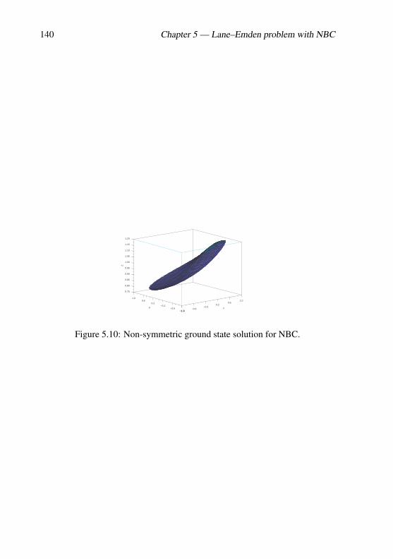
140 Chapter 5 — Lane–Emden problem with NBC
0.75
0.80
0.85
0.90
0.95
1.00
1.05
1.10
1.15
1.20
Z
−1.0−0.6
−0.20.2
0.61.0
Y−1.0
−0.6−0.2
0.20.6
1.0
X
Figure 5.10: Non-symmetric ground state solution for NBC.
Chapter 6
General potentials: mountainpass algorithms
In this last chapter, we consider the problem−∆u(x)+V (x)u(x) = f (u(x)), x ∈Ω,
u(x) = 0, x ∈ ∂Ω,(SP)
defined on an open bounded connected domain Ω in RN and N ≥ 2. We alsopay some attention to the case Ω = RN . Let us remark that, this time, thenonlinearity f is fixed and do not depend on a parameter p.
About the operator −∆+V , we assume that
(V1) V is continuous on Ω and 0 does not belong to the spectrum σ(−∆+V ).
Let us remark that we accept that the linear operator−∆+V possesses negativeeigenvalues. As zero does not belong to the spectrum of −∆ +V , we have thedecomposition H1
0 (Ω) = H(+)⊕H(−) corresponding to the positive and nega-tive eigenspaces of −∆ +V . For any u ∈ H1
0 (Ω), we can uniquely decomposeu = u(+) +u(−) in H(+)⊕H(−) such that∫
Ω
|∇u|2 +Vu2 =∫
Ω
|∇u(+)|2 +V (u(+))2 +∫
Ω
|∇u(−)|2 +V (u(−))2
with∫
Ω|∇u(+)|2 +V (u(+))2 ≥ 0 and
∫Ω|∇u(−)|2 +V (u(−))2 ≤ 0.
About f , we assume that
141
142 Chapter 6 — General potentials: mountain pass algorithms
(F1) f is continuous and subcritical, i.e. there exist a > 0 and p ∈ (2,2∗) suchthat, for any t ∈ R, | f (t)| ≤ a(1+ |t|p−1);
(F2) lim|t|→0f (t)
t = 0;
(F3) lim|t|→+∞
F(t)t2 →+∞;
(F4) t 7→ f (t)|t| is increasing on (−∞,0) and (0,+∞),
where F(t) :=∫ t
0 f (s)ds.Solutions of Problem (SP) are the critical points of the energy functional
E : H10 (Ω)→ R : u 7→ 1
2
∫Ω
(|∇u(x)|2 +V (x)u(x)2) dx−
∫Ω
F(u(x))dx. (6.1)
Let us point that the interesting feature of this problem is the fact that zerois not required to be a local minimum of E (cfr. directions in H(−) when H(−) 6=0). In this case, the mountain pass geometry does not hold anymore (seeFigure 1.1).
Recently, in [64], A. Szulkin and T. Weth proved that this problem possessesa non-trivial solution with minimum energy, i.e. a ground state solution. Let usjust remark that they do not need the usual super-quadraticity assumption (SQ).So, they generalize classical results of P. H. Rabinowitz (see e.g. [61]) where(SQ) was required.
(SQ) ∃a > 2, ∀u ∈ R\0, aF(u)≥ f (u)u > 0.
Moreover, they prove the existence of a ground state solution if one works withΩ = RN . One just needs to require in more some periodicity assumptions on fand V :
(PA) f and V are 1-periodic in xi, for i = 1, . . . ,N.
To obtain it, inspired by a result of A. Pankov [56], they introduce a variantof the classical Nehari manifold defined previously: a ground state solutionachieves the minimum of the energy functional E on the generalized Neharimanifold NG
NG :=
u ∈ H10 (Ω)\0 : 〈dE (u),v〉= 0, for any v ∈ H(−)
. (6.2)
So, in some sense, they remove “descent” directions in H(−). Moreover, theyprove the following properties.
143
1. The minimum of the energy E on NG is attained by a non-zero functionand is a critical point of E .
2. For each u ∈ H10 (Ω)\H(−), NG intersects
H∗(u) := R>0u⊕H(−) = R>0u(+)⊕H(−)
in one and only one function which is the unique point at which the func-tional E achieves its maximum on H∗(u).
3. The functionP : H1
0 (Ω)\H(−)→NG : u 7→ P(u)
such that E is maximum on H∗(u) at P(u) defines a continuous projec-tion on NG. Restricted to the unit sphere S+ of H(+), P|S+ defines anhomeomorphism between S+ and NG.
Let us just remark that techniques defined in Chapter 1 to study the asymp-totic behavior and symmetries are not working when H(−) is not the trivialspace 0. As we do not know the exact coefficients of the projection P onthe generalized Nehari manifold anymore, results 1.1.2 and 1.1.6 concerninga priori bounds cannot be used. Here, we are interested in the convergenceof a constrained steepest descent algorithm to approach a non-zero solution ofProblem (SP), i.e. a critical point of E on NG. We pay attention to the groundstate solutions and make a conjecture on their symmetries in the case where Vis constant and the nonlinearity f is a small power.
Let us now outline the numerical approach. To start, we recall what happensin the classical case where the mountain pass geometry is respected, i.e. H(−) =0.Classical case: The projection PN on the classical Nehari manifold N is justgiven by
PN (u) = t∗u,
with E (t∗u) = maxt>0 E (tu). In the former case, Y. Li and J. Zhou (see e.g. [71,72]) proved that accumulation points of the sequence obtained by the follow-ing algorithm (also called mountain pass algorithm) are non-zero solutions ofProblem (SP).
144 Chapter 6 — General potentials: mountain pass algorithms
Mountain Pass Algorithm (MPA). 1. Choose u0 ∈N and n← 0;
2. If ∇E (un) = 0, then stop;else, n← n+1 and compute
un+1 = PN
(un− sn
∇E (un)‖∇E (un)‖
),
where sn ∈ R+ \0 is defined such that
E (un+1)−E (un) <− sn
2‖∇E (un)‖
and is sufficiently large (see Section 6.1 for a precise definition of theterm “sufficiently”);
3. Go to step 2.
A priori, the solution may not be a ground state solution. Nevertheless, con-cerning problems where the ground state solutions are one-signed functions andwhere the one-signed solutions are unique up to the sign (e.g. the Lane–Emdenproblem, see [32]), we obtain that if an accumulation point is one-signed thenit is a ground state solution a posteriori.
To seek sign-changing solutions, one can define a projection PM from sign-changing functions in H1
0 (Ω) to the nodal Nehari set M (see Introduction ofChapter 1 for a definition) by
PM (u) = PN (u+)+PN (u−),
with u+ := max(u,0) and u− := min(u,0). If one replaces PN with PM in MPA,one obtains the modified mountain pass algorithm (MMPA, see e.g. [25]). Inpractice, the MMPA seems to converge up to a subsequence to sign-changingcritical points of E . Nevertheless, to our knowledge, there is no proof of conver-gence. In two words, the problem is related to the fact that M is not a manifoldanymore and to the “bad” properties of PM . It will be explained later in detail(see Lemma 6.1.9). An open question is the definition of a “good” projectionPM ensuring a convergence of the constrained steepest descent algorithm. Letus remark that other algorithms have been studied with the aim to approachcritical points of E . For example, in 2001, the “high linking algorithm” (see
145
e.g. [25, 41]) has been introduced: starting from a “MPA” solution, it permitsto compute critical points of E with higher energy but, as for MMPA, the con-vergence is not established. An other one is a bissection method introduced byV. Barutello and S. Terracini (see e.g. [9, 10]). A proof of the convergence isgiven but, in practice, the algorithm requires to “know” a priori some levels ofE , which is not so easy to obtain.
Generalized case: In the case of Problem (SP) where H(−) may be differ-ent from 0, we introduce a generalized mountain pass algorithm: we provethat if one replaces PN with P in the MPA (see page 142), the algorithm iswell-defined, “stable” and converges. Moreover, any accumulation point is asolution of Problem (SP). Let us mention that the convergence of the algorithmdepends on the structure of the energy functional E and not directly on Prob-lem (SP). In some sense, the Problem (SP) is just an example. This is why, inSection 6.1, we work with general Hilbert space and general functional E . Wegive assumptions on E such that the generalized mountain pass algorithm con-verges to a non-zero critical point of E . The proof draw its inspiration from thepaper [66] written by N. Tacheny and C. Troestler. There, the authors were in-terested in the convergence up to a subsequence of a mountain pass algorithmunder some additional restrictions: they were looking for solutions in somecones of H1
0 (Ω). An interesting fact of [66] is a precise definition of allowedstepsize sn in the MPA (see page 142) in such a way one can control in somesense E (un− sn
∇un‖∇un‖ ). This is an important ingredient to obtain the conver-
gence up to a subsequence. Here, we improve the method by defining a newstepsize sn for the MPA in order to control E (un− s ∇un
‖∇un‖ ) for any 0 < s < sn.It allows us to obtain, in Section 6.1.2 and under a “localization” assumptionabout a critical point, the convergence of the algorithm. Let us remark that, asground state solutions can be sign-changing solutions and as we do not havethe uniqueness of the solution, we cannot verify anymore a posteriori whethersolutions are ground state solutions or not. Nevertheless, a steepest descentmethod increases the likelyhood that they are. We also study what happens inthe case where Ω = RN .
To conclude the chapter, we use the generalized MPA to make a conjectureabout the symmetries of ground state solutions if V = λ < −λ1 is a constantfunction with λi (resp. Ei) the eigenvalues (resp. eigenspaces) of −∆ in H1
0 (Ω)
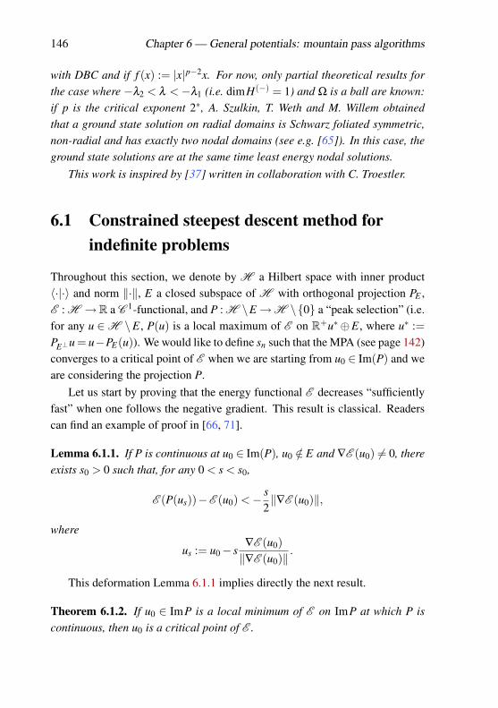
146 Chapter 6 — General potentials: mountain pass algorithms
with DBC and if f (x) := |x|p−2x. For now, only partial theoretical results forthe case where −λ2 < λ <−λ1 (i.e. dimH(−) = 1) and Ω is a ball are known:if p is the critical exponent 2∗, A. Szulkin, T. Weth and M. Willem obtainedthat a ground state solution on radial domains is Schwarz foliated symmetric,non-radial and has exactly two nodal domains (see e.g. [65]). In this case, theground state solutions are at the same time least energy nodal solutions.
This work is inspired by [37] written in collaboration with C. Troestler.
6.1 Constrained steepest descent method forindefinite problems
Throughout this section, we denote by H a Hilbert space with inner product〈·|·〉 and norm ‖·‖, E a closed subspace of H with orthogonal projection PE ,E : H →R a C 1-functional, and P : H \E→H \0 a “peak selection” (i.e.for any u ∈H \E, P(u) is a local maximum of E on R+u∗⊕E, where u∗ :=PE⊥u = u−PE(u)). We would like to define sn such that the MPA (see page 142)converges to a critical point of E when we are starting from u0 ∈ Im(P) and weare considering the projection P.
Let us start by proving that the energy functional E decreases “sufficientlyfast” when one follows the negative gradient. This result is classical. Readerscan find an example of proof in [66, 71].
Lemma 6.1.1. If P is continuous at u0 ∈ Im(P), u0 /∈ E and ∇E (u0) 6= 0, thereexists s0 > 0 such that, for any 0 < s < s0,
E (P(us))−E (u0) <− s2‖∇E (u0)‖,
where
us := u0− s∇E (u0)‖∇E (u0)‖
.
This deformation Lemma 6.1.1 implies directly the next result.
Theorem 6.1.2. If u0 ∈ ImP is a local minimum of E on ImP at which P iscontinuous, then u0 is a critical point of E .
6.1 — Constrained steepest descent method 147
Proof. If u0 were not a critical point of E , i.e. ∇E (u0) 6= 0, Lemma 6.1.1 wouldimply the existence of a s0 > 0 such that, for any s ∈ (0,s0),
E (P(us)) < E (u0)−s2‖∇E (u0)‖< E (u0),
which is, for s small, a contradiction with the definition of local minimum.
In fact, we can improve the deformation Lemma 6.1.1 and obtain the fol-lowing uniform deformation Lemma 6.1.3. This result gives a local uniformityaround u0. It will be a key to obtain the convergence of the algorithm.
Lemma 6.1.3. If P is continuous at u0 ∈ Im(P), u0 /∈ E and ∇E (u0) 6= 0, thereexist s0 > 0 and r0 > 0 such that, for any 0 < s≤ s0 and u∈ B(u0,r0), ∇E (u) 6=0, us 6= 0 where us := u− s ∇E (u)
‖∇E (u)‖ and
E (P(us))−E (u) <− s2‖∇E (u)‖.
Proof. First, there exists ε0 > 0 such that zero does not belong to B(u0,ε0) and,for any u∈ B(u0,ε0), ∇E (u) 6= 0. In fact, we can assume there exists c > 0 suchthat, for any u ∈ B(u0,ε0), ‖u‖ ≥ c and ‖∇E (u)‖ ≥ c.
Let 0 < ε1 < 12 ε0, for any u ∈ B(u0,ε1) and v ∈ B(u,ε1), we have v ∈
B(u0,ε0). So, for any u ∈ B(u0,ε1) and v ∈ B(u,ε1), zero does not belong toB(u,ε1), ‖v‖ ≥ c and ‖∇E (v)‖ ≥ c.
Second, let us consider du :=− ∇E (u)‖∇E (u)‖ . There exists α > 0 such that
⟨∇E (u0)|du0
⟩<−‖∇E (u0)‖√
2−α.
By continuity, possibly taking a smaller ε1, if ε2 < 12 ε1 then, for any u ∈
B(u0,ε2) and v ∈ B(u,ε2),
〈∇E (v)|du〉 ≤ −‖∇E (u)‖√
2.
Let ε3 < 14 ε2, there exist 2−1/2 < t1 < 1 < t2 such that, for any t ∈ (t1, t2),
s ∈ (0,ε3), u ∈ B(u0,ε3) and v ∈ B(0,ε3), the function tu + v + sdu belongs toB(u,ε2).
148 Chapter 6 — General potentials: mountain pass algorithms
By definition of P, for any u ∈ B(u0,ε3)∩ ImP, u maximizes E on
(t1u, t2u)⊕BE(0,ε3).
So, for any t ∈ (t1, t2), s ∈ (0,ε3), v ∈ BE(0,ε3) and u ∈ B(u0,ε3)∩ ImP, wehave, using the mean value theorem, that there exists σ ∈ (0,s)⊆ (0,ε3) suchthat
E (tu+ v+ sdu)−E (u)≤ E (tu+ v+ sdu)−E (tu+ v)
= 〈∇E (tu+ v+σdu)|sdu〉<−s√2‖∇E (u)‖.
As tus = tu + tsd, we have, for any t ∈ (t1, t2), 0 < s < ε3/t, v ∈ BE(0,ε3) andu ∈ B(u0,ε3) that
E (tus + v)−E (u) <−ts‖∇E (u)‖√
2<− s
2‖∇E (u)‖.
It remains to show that there exist s0 < 1t2
ε3 and r0 < ε3 such that, for any0 < s < s0 and u ∈ B(u0,r0),
P(us) ∈ (t1us, t2us)⊕BE(0,ε3) =: A.
If not, there would exist sn→ 0 and un→ u0 such that P(un + sndun) = tn(un +sndun)+ hn does not belong to A, where tn > 0 and hn ∈ E. On one hand, weobtain that PE⊥(P(un + sndun)) = tnPE⊥(un + sndun) converges to PE⊥u0. So, forlarge n, tn ∈ (t1, t2). On the other hand, PE(P(un + sndun)) = tnPE(un + sndun)+hn converges to PE(u0). So, for large n, hn ∈ B(0,r3), which is a contradiction.
So, there exist 0 < s0 < 1t2
ε3 and 0 < r0 < ε3 such that, for any 0 < s < s0
and u ∈ B(u0,r0), P(us) ∈ (t1us, t2us)⊕BE(0,ε3) and
E (P(us))−E (u) <− s2‖∇E (u)‖,
which concludes the proof.
Remark 6.1.4. The value 12 given in Lemma 6.1.3 is not optimal. It can be
changed by any number between 0 and 1 (excluded).
6.1 — Constrained steepest descent method 149
6.1.1 Convergence up to a subsequence
With the deformation Lemma 6.1.3, using the generalized MPA, it is possible toconstruct a stepsize sn such that the energy E is decreasing along the obtainedsequence (un)n∈N. Of course, without loss of generality, we can assume that∇E (un) 6= 0 for any n ∈ N (otherwise we directly get a critical point).
Proposition 6.1.5. If sn verifies the inequality about the energy functional givenin Lemma 6.1.3 for any n ∈ N, then the functional E decreases along the se-quence (un)n∈N.
Proof. As ∇E (un) 6= 0, sn > 0 by Lemma 6.1.3. By construction, we have
E (un+1)−E (un) = E
(P(un− sn
∇E (un)‖∇E (un)‖
))−E (un) <− sn
2‖∇E (un)‖< 0.
So, E (un+1) < E (un).
Nevertheless, this is not enough to obtain the convergence to a critical point:we must avoid sn being arbitrary close to zero without being “mandated” by thefunctional. To have it, let u0 ∈H \E and us = u0− s ∇E (u0)
‖∇E (u0)‖ , we set
S∗(u0) :=
s0 > 0 : ∀ 0 < s≤ s0, us 6= 0 and
E (P(us))−E (u0) <− s2‖∇E (u0)‖
and S(u0) := S∗(u0)∩
( 12 supS∗(u0),+∞
).
The set S∗(u0) is always defined and not-empty as soon as u0 is not a criticalpoint of E (thanks to the deformation lemma). Concerning S(u0), it is not-empty once E is bounded from below on ImP.
We consider the following generalized mountain pass algorithm:
Algorithm 6.1.6. 1. Choose u0 ∈ ImP and n← 0;
2. If ∇E (un) = 0, then stop;else, n← n+1 and compute
un+1 = P(
un− sn∇E (un)‖∇E (un)‖
),
where sn ∈ S(un);
150 Chapter 6 — General potentials: mountain pass algorithms
3. Go to step 2.
The following result gives a “stablility” and uniformity of the algorithm.
Lemma 6.1.7. If u0 ∈ ImP, ∇E (u0) 6= 0 and P is continuous at u0, then thereexists an open neighbourhood V of u0 and s∗ > 0 such that S(u)⊆ [s∗,+∞), forany u ∈V ∩ ImP.
Proof. By the uniform deformation Lemma 6.1.3, there exists s0 > 0 and r0 >
0 such that, for any 0 < s ≤ s0 and u ∈ B(u0,r0), we have u− s ∇E (u)‖∇E (u)‖ 6= 0,
∇E (u) 6= 0 and
E
(P(u− s
∇E (u)‖∇E (u)‖
))−E (u) <− s
2‖∇E (u)‖.
So, for any u ∈ B(u0,r0), s0 ∈ S∗(u). It follows that S(u)⊆ ( s02 ,+∞). It suffices
to take s∗ < s0/2.
The result 6.1.9 is a key to obtain the proof of the convergence up to asubsequence. Before proving that result, let us establish the following lemma.
Lemma 6.1.8. Let c > 0. For any u,v ∈H such that ‖u‖ ≥ c and ‖v‖ ≥ c,∥∥∥∥ u‖u‖− v‖v‖
∥∥∥∥≤ c−1‖u− v‖.
Proof. This is an immediate consequence of the following simple calculation:∥∥∥∥ u‖u‖− v‖v‖
∥∥∥∥2
= 2−2〈u|v〉‖u‖‖v‖
=1
‖u‖‖v‖(2‖u‖‖v‖−2〈u|v〉)
≤ 1‖u‖‖v‖
(‖u‖2 +‖v‖2−2〈u|v〉)
=‖u− v‖2
‖u‖‖v‖.
Lemma 6.1.9. Let (un)n∈N and (sn)n∈N given by the generalized MPA 6.1.6.Assume that infu∈ImP‖PE⊥u‖> 0 and that P is continuous.If ∑
+∞
n=0 sn < +∞ then (un)n∈N converges in H .
6.1 — Constrained steepest descent method 151
Proof. To simplify the notations, we denote u∗ := PE⊥u. Let vn := u∗n‖u∗n‖
, a :=
infu∈ImP‖u∗‖> 0 and dn :=− ∇E (un)‖∇E (un)‖ .
First, as ‖u∗n‖ ≥ a > 0 and there exists n0 such that, for any n≥ n0, sn < a2 ,
we have
‖u∗n + snd∗n‖ ≥ ‖u∗n‖− sn‖d∗n‖ ≥ ‖u∗n‖− sn ≥a2
=: b > 0.
Second, for any n ∈ N, there exists tn > 0 and hn ∈ E such that
vn+1 =(P(un + sndn))∗
‖(P(un + sndn))∗‖=
(tnun + tnsndn +hn)∗
‖(tnun + tnsndn +hn)∗‖
=tnu∗n + tnsnd∗n‖tnu∗n + tnsnd∗n‖
=u∗n + snd∗n‖u∗n + snd∗n‖
.
So, for any n > n0, by Lemma 6.1.8, we have
‖vn+1− vn‖ ≤ 2b−1‖snd∗n‖ ≤ 2b−1sn.
So, (vn)n∈N is a Cauchy sequence. As P(vn) = P(u∗n) = un, by continuity of P,(un)n∈N converges.
Remark 6.1.10. In the previous proof of Lemma 6.1.9, if we wanted to workwith the projection on the nodal Nehari set PM defined in the Introduction ofthis chapter, we could not remove the projection in the computation of vn+1.This explains why the proof of convergence is not known at the moment in thiscase.
Theorem 6.1.11. If zero does not belong to ImP, P is continuous, E satisfiesthe Palais-Smale condition in ImP and infu∈ImP E (u) >−∞, then (un)n∈N givenby the generalized mountain pass algorithm 6.1.6 possesses a subsequence con-verging to a critical point of E . Moreover, all accumulation points of (un)n∈Nare critical points of E .
Proof. Let us start by showing that (∇E (un))n∈N converges to zero up to asubsequence. If not, we could assume there exists δ > 0 and n0 ∈ N such that,for any n≥ n0, ‖∇E (un)‖> δ . Then, for any n≥ n0, we have
E (un+1)−E (un)≤−12
snδ .
152 Chapter 6 — General potentials: mountain pass algorithms
Thus, by adding up,
limn→N
E (un)−E (un0) =+∞
∑n=n0
E (un+1)−E (un)≤−δ
2
+∞
∑n=n0
sn.
On one hand, as the left-hand side is a real number (E is bounded from below onImP and decreasing on (un)n∈N), we have ∑
+∞
n=0 sn < +∞. So, by Lemma 6.1.9,un→ u∗ ∈ ImP and ‖∇E (u∗)‖ ≥ δ . On the other hand, by continuity of P, wehave P(u∗) = u∗ and, so, u∗ ∈ ImP. By Lemma 6.1.7, there exists a neighbour-hood V of u∗ and s∗ > 0 such that S(u) ⊆ [s∗,+∞), for any u ∈ V . So, thereexists n0 such that, for any n ≥ n0, sn ≥ s∗ whence ∑
+∞
n=0 sn does not converge,which is a contradiction.
Therefore, there exists a sequence (unk)k∈N ⊆ (un)n∈N such that ‖∇E (unk)‖converges to 0 when k → +∞. As E satisfies the Palais-Smale condition,(unk)k∈N possesses a subsequence converging to a critical point of E .
Concerning the second statement of the thesis, the argument is very similar.Let (unk)k∈N be a convergent subsequence and assume on the contrary that u =limk→∞ unk is not a critical point of E . In that case, on one hand, there existsδ > 0 and k1 ∈ N such that, for any k ≥ k1, ‖∇E (unk)‖ ≥ δ . By Lemma 6.1.3,we have
∀k ≥ k1, E (unk+1)−E (unk)≤−12
δ snk .
On the other hand, as u ∈ ImP, we have by Lemma 6.1.7 that
∃ s∗ > 0, ∃k2 ∈ N, ∀k ≥ k2, sn ≥ s∗.
So, for large k, E (unk+1)−E (unk) ≤ −14 δ s∗, which is a contradiction because
(E (un))n∈N is a convergent sequence.
6.1.2 Convergence
In this section, under a “localization” assumption, we prove that the entire se-quence (un)n∈N given by the generalized mountain pass algorithm 6.1.6 con-verges to a non-zero solution of Problem (SP). It explains why we changed thedefinition of the stepsize sn given in the paper [66].
Assume that we are able to locate a non-zero solution u of Problem (SP)with the following property: u is the unique critical point of E in the ballB(u,δ ), for some δ > 0. Let us denote S(u,r) := v : ‖v−u‖= r.
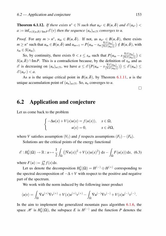
6.2 — Application and conjecture 153
Theorem 6.1.12. If there exists n∗ ∈ N such that un∗ ∈ B(u,δ ) and E (un∗) <
a := infv∈S(u,δ )∩ImP E (v) then the sequence (un)n∈N converges to u.
Proof. For any m > n∗, um ∈ B(u,δ ). If not, as un∗ ∈ B(u,δ ), there existsm≥ n∗ such that um ∈ B(u,δ ) and um+1 = P
(um− sm
∇E (um)‖∇E (um)‖
)/∈ B(u,δ ), with
sm ∈ S(um).So, by continuity, there exists 0 < s ≤ sm such that P
(um− s ∇E (um)
‖∇E (um)‖)∈
S(u,δ )∩ ImP. This is a contradiction because, by the definition of sm and asE is decreasing on (un)n∈N, we have a ≤ E
(P(um− s ∇E (um)
‖∇E (um)‖ ))≤ E (um) ≤
E (un∗) < a.As u is the unique critical point in B(u,δ ), by Theorem 6.1.11, u is the
unique accumulation point of (un)n∈N. So, un converges to u.
6.2 Application and conjecture
Let us come back to the problem−∆u(x)+V (x)u(x) = f (u(x)), x ∈Ω,
u(x) = 0, x ∈ ∂Ω,
where V satisfies assumption (V1) and f respects assumptions (F1)− (F4).Solutions are the critical points of the energy functional
E : H10 (Ω)→ R : u 7→ 1
2
∫Ω
(|∇u(x)|2 +V (x)u(x)2) dx−
∫Ω
F(u(x))dx, (6.3)
where F(u) :=∫ u
0 f (s)ds.Let us denote the decomposition H1
0 (Ω) = H(−)⊕H(+) corresponding tothe spectral decomposition of −∆+V with respect to the positive and negativepart of the spectrum.
We work with the norm induced by the following inner product
〈u|v〉=∫
Ω
∇u(+)∇v(+) +V (x)u(+)v(+)−
∫Ω
∇u(−)∇v(−) +V (x)u(−)v(−).
In the aim to implement the generalized mountain pass algorithm 6.1.6, thespace H is H1
0 (Ω), the subspace E is H(−) and the function P denotes the
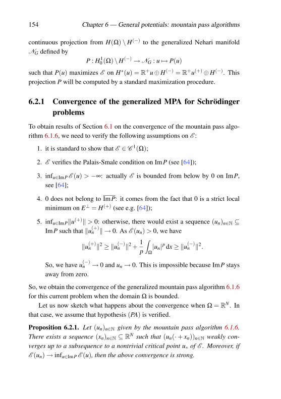
154 Chapter 6 — General potentials: mountain pass algorithms
continuous projection from H(Ω) \H(−) to the generalized Nehari manifoldNG defined by
P : H10 (Ω)\H(−)→NG : u 7→ P(u)
such that P(u) maximizes E on H∗(u) = R+u⊕H(−) = R+u(+)⊕H(−). Thisprojection P will be computed by a standard maximization procedure.
6.2.1 Convergence of the generalized MPA for Schrödingerproblems
To obtain results of Section 6.1 on the convergence of the mountain pass algo-rithm 6.1.6, we need to verify the following assumptions on E :
1. it is standard to show that E ∈ C 1(Ω);
2. E verifies the Palais-Smale condition on ImP (see [64]);
3. infu∈ImP E (u) > −∞: actually E is bounded from below by 0 on ImP,see [64];
4. 0 does not belong to ImP: it comes from the fact that 0 is a strict localminimum on E⊥ = H(+) (see e.g. [64]);
5. infu∈ImP‖u(+)‖ > 0: otherwise, there would exist a sequence (un)n∈N ⊆ImP such that ‖u(+)
n ‖→ 0. As E (un) > 0, we have
‖u(+)n ‖2 ≥ ‖u(−)
n ‖2 +1p
∫Ω
|un|p dx≥ ‖u(−)n ‖2.
So, we have u(−)n → 0 and un→ 0. This is impossible because ImP stays
away from zero.
So, we obtain the convergence of the generalized mountain pass algorithm 6.1.6for this current problem when the domain Ω is bounded.
Let us now sketch what happens about the convergence when Ω = RN . Inthat case, we assume that hypothesis (PA) is verified.
Proposition 6.2.1. Let (un)n∈N given by the mountain pass algorithm 6.1.6.There exists a sequence (xn)n∈N ⊆ RN such that (un(·+ xn))n∈N weakly con-verges up to a subsequence to a nontrivial critical point u∗ of E . Moreover, ifE (un)→ infu∈ImP E (u), then the above convergence is strong.
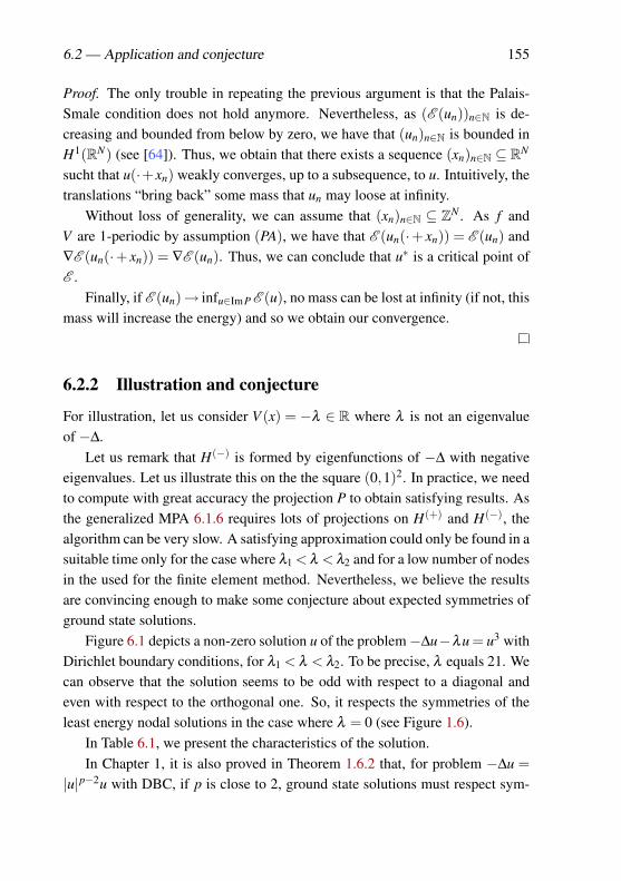
6.2 — Application and conjecture 155
Proof. The only trouble in repeating the previous argument is that the Palais-Smale condition does not hold anymore. Nevertheless, as (E (un))n∈N is de-creasing and bounded from below by zero, we have that (un)n∈N is bounded inH1(RN) (see [64]). Thus, we obtain that there exists a sequence (xn)n∈N ⊆ RN
sucht that u(·+xn) weakly converges, up to a subsequence, to u. Intuitively, thetranslations “bring back” some mass that un may loose at infinity.
Without loss of generality, we can assume that (xn)n∈N ⊆ ZN . As f andV are 1-periodic by assumption (PA), we have that E (un(·+ xn)) = E (un) and∇E (un(·+ xn)) = ∇E (un). Thus, we can conclude that u∗ is a critical point ofE .
Finally, if E (un)→ infu∈ImP E (u), no mass can be lost at infinity (if not, thismass will increase the energy) and so we obtain our convergence.
6.2.2 Illustration and conjecture
For illustration, let us consider V (x) = −λ ∈ R where λ is not an eigenvalueof −∆.
Let us remark that H(−) is formed by eigenfunctions of −∆ with negativeeigenvalues. Let us illustrate this on the the square (0,1)2. In practice, we needto compute with great accuracy the projection P to obtain satisfying results. Asthe generalized MPA 6.1.6 requires lots of projections on H(+) and H(−), thealgorithm can be very slow. A satisfying approximation could only be found in asuitable time only for the case where λ1 < λ < λ2 and for a low number of nodesin the used for the finite element method. Nevertheless, we believe the resultsare convincing enough to make some conjecture about expected symmetries ofground state solutions.
Figure 6.1 depicts a non-zero solution u of the problem−∆u−λu = u3 withDirichlet boundary conditions, for λ1 < λ < λ2. To be precise, λ equals 21. Wecan observe that the solution seems to be odd with respect to a diagonal andeven with respect to the orthogonal one. So, it respects the symmetries of theleast energy nodal solutions in the case where λ = 0 (see Figure 1.6).
In Table 6.1, we present the characteristics of the solution.In Chapter 1, it is also proved in Theorem 1.6.2 that, for problem −∆u =
|u|p−2u with DBC, if p is close to 2, ground state solutions must respect sym-
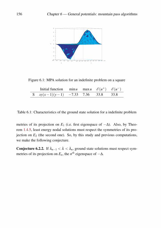
156 Chapter 6 — General potentials: mountain pass algorithms
−8
−6
−4
−2
0
2
4
6
8
Z
0.0 0.1 0.2 0.3 0.4 0.5 0.6 0.7 0.8 0.9 1.0
Y
0.0 0.2 0.4 0.6 0.8 1.0
X
Figure 6.1: MPA solution for an indefinite problem on a square
Initial function minu maxu E (u+) E (u−)S xy(x−1)(y−1) −7.33 7.36 33.8 33.8
Table 6.1: Characteristics of the ground state solution for a indefinite problem
metries of its projection on E1 (i.e. first eigenspace of −∆). Also, by Theo-rem 1.4.5, least energy nodal solutions must respect the symmetries of its pro-jection on E2 (the second one). So, by this study and previous computations,we make the following conjecture.
Conjecture 6.2.2. If λn−1 < λ < λn, ground state solutions must respect sym-metries of its projection on En, the nth eigenspace of −∆.
Appendix A
Some classical results
In this appendix, we only list some important results used several timesduring the proofs presented in this work.
The two first results are classical in functional analysis. We mainly usedthem to apply the Lebesgue’s dominated convergence theorem or to prove theconvergence of some sequences.
Proposition A.1. Let (un)n∈N be a sequence of the Banach space X and u ∈X . If, from any subsequence (vn)n∈N of (un)n∈N, there exists a subsequence(wn)n∈N of (vn)n∈N converging to u, then un converges to u.
Proposition A.2. Let 1 ≤ p < +∞. If un → u in Lp(Ω) then, up to a subse-quence, there exists f ∈ Lp(Ω) such that |un| ≤ f almost everywhere.
The following results are classical in the Sobolev space theory. To start, wegive a characterization of λn, the eigenvalues of −∆. This result is called thePoincaré’s principle. Let us fix Ei the eigenspaces related to λi.
Theorem A.3. For any n ∈ N,
λn = min∫
Ω
|∇u|2 : u ∈ H10 (Ω),
∫Ω
u2 dx = 1,∫Ω
ue1 dx = · · ·=∫
Ω
uen−1 = 0,
for any ei ∈ Ei.
157
158 Appendix A — Some classical results
Also due to H. Poincaré, we can work with “more general” Sobolev spaces.
Theorem A.4. Let Ω be an open bounded domain of RN and 1 ≤ q < +∞.There exists a positive constant C such that, for any1 u ∈W 1,q
0 (Ω),
‖u‖q ≤C‖∇u‖q.
The two following results give the Sobolev’s embeddings.
Theorem A.5. If 1 ≤ p < N, then there exists a positive constant C such that,for any test functions2 u,
‖u‖L
pNN−p≤C‖∇u‖Lp .
Theorem A.6. • Let Ω⊆ RN be a domain respecting the cone condition3.If 1≤ q < N and q≤ s≤ qN
N−q then W 1,q(Ω)⊆ Ls(Ω) and the embeddingis continuous.
• Let Ω ⊆ RN be a local Lipschitz domain. If N < q < +∞ then W 1,q ⊆C (Ω) and the embedding is continuous.
The last one gives to us the Rellich’s embedding.
Theorem A.7. • Let Ω ⊆ RN be a domain respecting the cone condition.If 1 ≤ q < N and 1 ≤ s < q∗ = qN
N−q then W 1,q(Ω) ⊆ Ls(Ω) and the em-bedding is compact.
• Let Ω ⊆ RN be a local Lipschitz domain. If N < q < +∞ then W 1,q ⊆C (Ω) and the embedding is compact.
Let us remark that if we are working with spaces W 1,q0 (Ω), the conclusions
of theorems A.6 and A.7 are valid for any domains Ω. Readers can find a proofin [2].
1Closure in Lq(Ω) of the space C 20 (Ω) for the classical norm (
∫Ω|∇u|q)1/q.
2Functions in C +∞ with compact support.3There exists a finite cone K such that each point x∈Ω is the vertex of a finite cone Kx contained
in Ω and congruent to K.
Notations
∆ Laplacian operator
∇ Gradient operator
div Divergence operator
H(Ω) Sobolev space H10 (Ω)(resp. H1(Ω))
depending on Problem with DBC (resp. NBC)
H H(Ω) in short
‖u‖2∫
Ω
|∇u|2 in H10 (Ω) or
∫Ω
|∇u|2 +u2 in H1(Ω)
λi ith eigenvalue in H of −∆ with DBC or −∆+ id with NBC
Ei Eigenspace related to λi
ei Eigenfunction in Ei with ‖ei‖= 1
‖u‖p Traditional norm in Lp:(∫
Ω
|u|p)1/p
‖.‖X Traditional norm in X
S Unit sphere of H
SN Unit sphere of RN
S(a,r) Sphere centered in a with radius r in H
B Unit ball of H
BN Unit ball of RN
B(a,r) Open ball centered in a with radius r in H
159
160 Notations
B[a,r] Closed ball centered in a with radius r in H
〈u|v〉 Inner product in H:∫
Ω
∇u∇v if H10 (Ω) and∫
Ω
∇u∇v+uv if H1(Ω), unless said otherwise
f ′(.) Derivative of f : R→ R
dE (.) Frechet derivative of E
〈dE (u),v〉 Derivative of E at u taken in the direction v
〈d2E (u),v,w〉 Second derivative of E at u taken in the directions v and w
∂uE Partial derivative of E related to u
X⊥ Orthogonal space of X in H
PX Orthogonal projection from H to X
d(A,B) Distance between A and B
∂A Boundary of A
X′
Dual space of X (continuous and linear functionals)
u+ max(0,u)
u− min(0,u)
b Compact embedding
A Closure of set A
∂ν Derivative in the outer normal direction
M(R) Set of Borel-measurable functions from R to R
C (X) Set of continuous functions from X to R
C n(X) Set of fns n times continuous differentiable from X to R
C n(X ,Y ) Set of fns n times continuous differentiable from X to Y
C n0 (X) Set of fns n times differentiable with compact support
C 1,α C 1-functions with α-Hölder continuous derivative
C 1,αloc C 1-functions with α-Hölder continuous derivative
on any compact
σ( f ) Spectrum of operator f

Notations 161
Im( f ) Image of f

162 Notations
Bibliography
[1] Milton Abramowitz and Irene A. Stegun. Handbook of mathematical func-tions with formulas, graphs, and mathematical tables, volume 55 of Na-tional Bureau of Standards Applied Mathematics Series. For sale by theSuperintendent of Documents, U.S. Government Printing Office, Wash-ington, D.C., 1964.
[2] Robert A. Adams. Sobolev spaces. Academic Press [A subsidiary ofHarcourt Brace Jovanovich, Publishers], New York-London, 1975. Pureand Applied Mathematics, Vol. 65.
[3] Amandine Aftalion and Filomena Pacella. Qualitative properties of nodalsolutions of semilinear elliptic equations in radially symmetric domains.C. R. Math. Acad. Sci. Paris, 339(5):339–344, 2004.
[4] Götz Alefeld, Andreas Frommer, Gerhard Heindl, and Jan Mayer. Onthe existence theorems of Kantorovich, Miranda and Borsuk. ElectronicTransactions on Numerical Analysis, 17:102–111, 2004.
[5] Giovanni Alessandrini. Nodal lines of eigenfunctions of the fixed mem-brane problem in general convex domains. Comment. Math. Helv.,69(1):142–154, 1994.
[6] Antonio Ambrosetti and Paul H. Rabinowitz. Dual variational methods incritical point theory and applications. J. Functional Analysis, 14:349–381,1973.
163
164 BIBLIOGRAPHY
[7] Aomar Anane and Najib Tsouli. On the second eigenvalue of the p-Laplacian. Nonlinear partial differential equations (Fés, 1994) PitmanRes. Notes Math. Ser., 343:1–9, 1996.
[8] Thomas Bartsch, Tobias Weth, and Michel Willem. Partial symmetry ofleast energy nodal solutions to some variational problems. J. Anal. Math.,96:1–18, 2005.
[9] Vivina Barutello. On the n-body problem. Phd thesis, Universita Milano-Bicocca, Italia, 2004.
[10] Vivina Barutello and Susanna Terracini. A bisection algorithm for thenumerical mountain pass. NoDEA Nonlinear Differential Equations Appl.,14(5-6):527–539, 2007.
[11] Marino Belloni and Bernd Kawohl. A direct uniqueness proof forequations involving the p-Laplace operator. Manuscripta mathematica,109:229–231, 2002.
[12] Denis Bonheure, Vincent Bouchez, and Christopher Grumiau. Asymp-totics and symmetries of ground-state and least energy nodal solutions forboundary-value problems with slowly growing superlinearities. Differen-tial Integral Equations, 22(9-10):1047–1074, 2009.
[13] Denis Bonheure, Vincent Bouchez, and Christopher Grumiau. Lane–emden problem with neumann conditions: symmetries of ground statesolutions. Preprint, 2010.
[14] Denis Bonheure, Vincent Bouchez, Christopher Grumiau, and JeanVan Schaftingen. Asymptotics and symmetries of least energy nodal so-lutions of Lane-Emden problems with slow growth. Commun. Contemp.Math., 10(4):609–631, 2008.
[15] Denis Bonheure, Enrico Serra, and Massimo Tarallo. Symmetry of opti-mal functions in Moser-Trudinger inequalities and a hénon type problemin dimension two. Advances in Differential Equations, 13(1-2):105–138,2008.
BIBLIOGRAPHY 165
[16] Timothy H. Boyer. Concerning the zeros of some functions related toBessel functions. J. Mathematical Phys., 10:1729–1744, 1969.
[17] B. Breuer, Jiri Horák, P. Joseph McKenna, and Michael Plum. Acomputer-assisted existence and multiplicity proof for travelling waves ina nonlinearly supported beam. J. Differential Equations, 224(1):60–97,2006.
[18] B. Breuer, P. Joseph McKenna, and Michael Plum. Multiple solutions fora semilinear boundary value problem: a computational multiplicity proof.J. Differential Equations, 195(1):243–269, 2003.
[19] Haïm Brezis. Analyse fonctionnelle. Collection Mathématiques Ap-pliquées pour la Maîtrise. [Collection of Applied Mathematics for theMaster’s Degree]. Masson, Paris, 1983. Théorie et applications. [Theoryand applications].
[20] Haïm Brézis and Louis Nirenberg. Positive solutions of nonlinear ellipticequations involving critical Sobolev exponents. Comm. Pure Appl. Math.,36(4):437–477, 1983.
[21] Robert F. Brown. A topological introduction to nonlinear analysis.Birkhäuser Boston Inc., Boston, MA, 1993.
[22] Eric Cancès, Claude Le Bris, and Yvon Maday. Méthodes mathématiquesen chimie quantique. Une introduction, volume 53 of Mathématiques &Applications (Berlin) [Mathematics & Applications]. Springer, Berlin,2006.
[23] Alfonso Castro, Jorge Cossio, and John M. Neuberger. A sign-changingsolution for a superlinear Dirichlet problem. Rocky Mountain J. Math.,27(4):1041–1053, 1997.
[24] Yung Sze Choi and P. Joseph McKenna. A mountain pass method forthe numerical solution of semilinear elliptic problems. Nonlinear Anal.,20(4):417–437, 1993.
166 BIBLIOGRAPHY
[25] David G. Costa, Zhonghai Ding, and John M. Neuberger. A numericalinvestigation of sign-changing solutions to superlinear elliptic equationson symmetric domains. J. Comput. Appl. Math., 131(1-2):299–319, 2001.
[26] Emmanuele Dibenedetto. C 1,α -local regularity of weak solutions of de-generate elliptic equations. Nonlinear analysis, 7:827–850, 1983.
[27] Alexandre Ern and Jean-Luc Guermond. Theory and practice of finiteelements. Applied Mathematical Sciences 159. New York, NY: Springer.xiii, 524 p., 2004.
[28] Julian Fernández Bonder, Enrique Lami Dozo, and Julio D. Rossi. Sym-metry properties for the extremals of the Sobolev trace embedding. Ann.Inst. H. Poincaré Anal. Non Linéaire, 21(6):795–805, 2004.
[29] Jesús P. Garcia Azorero and Ireneo Peral. Existence and nonuniquenessfor the p-Laplacian: nonlinear eigenvalues. Communications in PartialDifferential Equations, 12:1389–1430, 1987.
[30] Leszek Gasinski and Nikolaos S. Papageorgiou. Nonlinear analysis.Chapman & Hall / CRC, 2005.
[31] Marita Gazzini and Enrico Serra. The Neumann problem for the Hénonequation, trace inequalities and Steklov eigenvalues. Ann. Inst. H.Poincaré Anal. Non Linéaire, 25(2):281–302, 2008.
[32] Basilis Gidas, Wei Ming Ni, and Louis Nirenberg. Symmetry and relatedproperties via the maximum principle. Comm. Math. Phys., 68(3):209–243, 1979.
[33] David Gilbarg and Neil S. Trudinger. Elliptic partial differential equationsof second order. Classics in Mathematics. Springer-Verlag, Berlin, 2001.Reprint of the 1998 edition.
[34] Tomas Godoy, Jean-Pierre Gossez, and Sofia R. Paczka. A minimax for-mula for the principal eigenvalues of Dirichlet problems and its applica-tions. In Proceedings of the 2006 International Conference in honor ofJacqueline Fleckinger, volume 16 of Electron. J. Differ. Equ. Conf., pages
BIBLIOGRAPHY 167
137–154. Texas State Univ.–San Marcos, Dept. Math., San Marcos, TX,2007.
[35] Christopher Grumiau. Solution nodale d’énergie minimale. Master’s the-sis, Université de Mons-Hainaut, 2007.
[36] Christopher Grumiau and Enea Parini. On the asymptotics of solutionsof the Lane-Emden problem for the p-Laplacian. Arch. Math. (Basel),91(4):354–365, 2008.
[37] Christopher Grumiau and Christophe Troestler. Mountain-pass algorithmfor some indefinite problems. preprint, 2009.
[38] Christopher Grumiau and Christophe Troestler. Nodal line structure ofleast energy nodal solutions for Lane-Emden problems. C. R. Math. Acad.Sci. Paris, 347(13-14):767–771, 2009.
[39] Christopher Grumiau and Christophe Troestler. Oddness of least energynodal solutions on radial domains. Elec. Journal of diff. equations, Con-ference 18:23–31, 2010.
[40] Maria Hoffmann-Ostenhof, Thomas Hoffmann-Ostenhof, and NikolayNadirashvili. The nodal line of the second eigenfunction of the Lapla-cian in R2 can be closed. Duke Math. J., 90(3):631–640, 1997.
[41] Jirí Horák. Constrained mountain pass algorithm for the numerical solu-tion of semilinear elliptic problems. Numer. Math., 98(2):251–276, 2004.
[42] Yin Xi Huang. A note on the asymptotic behavior of positive solutions forsome elliptic equation. Nonlinear Analysis, 29:533–537, 1997.
[43] Klaus Jänich. Topology. Springer, 1984.
[44] Hubert Kalf. On the expansion of a function in terms of spherical harmon-ics in arbitrary dimensions. Bull. Belg. Math. Soc. Simon Stevin, 2(4):361–380, 1995.
[45] Dwayne L. Knirk. New developments in the application of hypersphericalcoordinates to atomic wave functions. Phys. Rev. Lett., 32:651–654, 1974.
168 BIBLIOGRAPHY
[46] Enrique J. Lami Dozo and Olaf Torné. Symmetry and symmetry break-ing for minimizers in the trace inequality. Commun. Contemp. Math.,7(6):727–746, 2005.
[47] Jonathan Homer Lane. On the theoretical temperature of the sun underthe hypothesis of a gaseous mass maintaining its volume by its internalheat and depending on the laws of gases known to terrestrial experiment.Americ. Jour. of Science and Arts, 2(50):57–74, 1870.
[48] Elsa M. Marchini. Techniques in the calculus of variations. Phd thesis,Universita Milano-bicocca, Italia, 2004.
[49] Jean Mawhin. Analyse. Accès Sciences. [Access to Sciences]. De BoeckUniversité, Brussels, second edition, 1997. Fondements, techniques, évo-lution. [Foundations, techniques, evolution].
[50] Jean Mawhin and Michel Willem. Critical Point Theory and HamiltonienSystems. Springer, New York, Heidelberg, London, Paris, Tokyo, 1989.
[51] Antonios D. Melas. On the nodal line of the second eigenfunction of thelaplacian in R2. J. Differential Geom., 35(1):255–263, 1992.
[52] Jurgen Moser. A Sharp Form of an Inequality by N. Trudinger. IndianaUniv. Math. J., 20:1077–1092, 1970/71.
[53] Claus Müller. Spherical harmonics, volume 17 of Lecture Notes in Math-ematics. Springer-Verlag, Berlin, 1966.
[54] John M. Neuberger. A numerical method for finding sign-changing so-lutions of superlinear dirichlet problems. Nonlinear World, 4(1):73–83,1997.
[55] Serge Nicaise. Analyse numérique et équations aux dérivées partielles.Sciences Sup, Dunod, Paris, 2000.
[56] Alexander Pankov. Periodic nonlinear Schrödinger equation with applica-tion to photonic crystals. Milan J. Math., 73:259–287, 2005.
BIBLIOGRAPHY 169
[57] Yehuda Pinchover and Jacob Rubinstein. An introduction to partial differ-ential equations, volume 17. Cambridge University PressSpringer-Verlag,Cambridge, 2005.
[58] Michael Plum and Christian Wieners. New solutions of the Gelfand prob-lem. J. Math. Anal. Appl., 269(2):588–606, 2002.
[59] Patrizia Pucci and James Serrin. The maximum principle. Progress inNonlinear Differential Equations and their Applications, 73. BirkhäuserVerlag, Basel, 2007.
[60] Paul H. Rabinowitz. Global Aspects of Bifurcation. Sém. Math. Sup.,91:63–112, 1985.
[61] Paul H. Rabinowitz. Minimax methods in critical point theory with ap-plications to differential equations, volume 65 of CBMS Regional Confer-ence Series in Mathematics. Published for the Conference Board of theMathematical Sciences, Washington, DC, 1986.
[62] Xiaofeng Ren and Juncheng Wai. Single-point condensation and least-energy solutions. Proceedings of the AMS, 124(1):111–120, 1996.
[63] Didier Smets, Jiabao Su, and Michel Willem. Non-radial ground states forthe Hénon equation. Commun. Contemp. Math., 4(3):467–480, 2002.
[64] Andrzej Szulkin and Tobias Weth. Ground state solutions for some indef-inite variational problems. J. Funct. Anal., 257(12):3802–3822, 2009.
[65] Andrzej Szulkin, Tobias Weth, and Michel Willem. Ground state solu-tions for a semilinear problem with critical exponent. Differential IntegralEquations, 22(9-10):913–926, 2009.
[66] Nicolas Tacheny and Christophe Troestler. A mountain pass algorithmwith projector. preprint, 2005.
[67] Oleg I. Tolstikhin and Michio Matsuzawa. Hyperspherical elliptic har-monics and their relation to the Heun equation. Pysical Review, 63, 2001.
170 BIBLIOGRAPHY
[68] Jean Van Schaftingen and Michel Willem. Partial symmetry of least en-ergy nodal solutions to some variational problems. J. Eur. Math. Soc.(JEMS), 10(2):439–456, 2008.
[69] Ni Wei-Ming and Takagi Izumi. On the neumann problem for some semi-linear elliptic equations and systems of activator-inhibitor type. Transac-tions of the american Mathematical society, 297(1):351–368, 1986.
[70] Michel Willem. Principes d’analyse fonctionnelle. Nouvelle BibliothèqueMathématique [New Mathematics Library], 9. Cassini, Paris, 2007.
[71] Jianxin Zhou and Youngxin Li. A minimax method for finding multi-ple critical points and its applications to semilinear elliptic pde’s. SIAMSci.Comp., 23:840–865, 2001.
[72] Jianxin Zhou and Youngxin Li. Convergence results of a local minimaxmethod for finding multiple critical points. SIAM Sci. Comp., 24:865–885,2002.
Index
AlgorithmMinimax, 149Mountain Pass, 29, 143, 149Steepest descent, 143
Assisted computer proof, 23, 60Asymptotic behavior
q-Laplacian, 90general nonlinearities, 100Lane–Emden Problem, 20, 37NBC, 123Schrödinger problem, 82
Barycenter, 20Bessel functions, 49, 50, 137Bifurcation
branch, 28, 121point, 28, 121
Borel-measurable function, 95Boundary conditions
Dirichlet, 16, 33Neumann, 16, 119
Constrained steepest descent method,29
ConvergenceC 0, 74C 1, 72
Critical points (def), 34
Deformation Lemma, 89, 146Degree theory, 122
Eigenfunctionson radial domains, 49, 137on the square, 59, 126
Eigenspaceof −∆+ id, 120of −∆, 19of Schrödinger operator, 80
Eigenvalueof −∆+ id , 120of −∆, 19of Schrödinger operator, 80
Elliptical regularity, 72, 82Energy functional, 16, 34, 80, 81, 95,
119, 153Entropy (def), 59
Finite element method, 30Fredholm alternative, 40, 92, 102, 123
Group action (def), 57
Hölder inequality, 42, 92, 93Höpf’s Lemma, 74
171
172 INDEX
Homogeneous polynomials, 50Hyperspherical coordinates, 49
Implicit function theorem, 36, 45, 52,105
Indefinite Problem, 141Interlacing property, 49, 51
Krasnoselskii genus, 82, 92Krasnoselskii-Boehme-Marino
Theorem, 121
l’Hôpital’s rule, 38Laplace operator, 16Lebesgue’s dominated
convergence, 41, 43, 44, 56,73, 94, 101, 109, 134
Lower bound for Lane–Emden Prob-lem, 41
Mean value theorem, 125, 134, 148Miranda theorem, 88Morse index, 121, 122Mountain pass structure, 17, 96, 142Moving planes method (def), 17
Nehari manifold, 35, 80, 86, 96, 120,142
Nehari manifoldReduced, 39, 98
Nodal line, 23, 71Nodal Nehari set, 35, 80, 86, 96Non homogeneous
nonlinearity, 25, 95Non-zero potential, 80, 84Nondegenerate case, 45
Operatorq-Laplacian, 25, 80Laplace-Beltrami, 49Positive definite, 24, 80
Palais-Smale condition, 119, 134Palais-Smale condition (def), 35Perturbation of Laplacian, 62, 79Poincaré inequality, 55, 105, 124Poincaré-Wirtinger
inequalities, 123Polar coordinates, 75Potential
Non-zero, 16, 24Problem
q-Laplacian, 81Lane–Emden, 16, 33, 119Schrödinger, 15, 79, 82
Projectionon Np, 102on an eigenspace, 23
Rabinowitz’s principle, 123Reduced Functional, 39, 98Rellich’s theorem, 43, 56Riez-Fischer characterization, 105
Scaling–renormalization, 33Separation of variables method, 49Sobolev inequality, 55, 96, 107Sobolev space
H1, 26, 119H1
0 , 16, 33W 1,q
0 , 25Sobolev’s embedding, 42, 72, 87, 88,
93
INDEX 173
SolutionGround state, 17, 67, 85Least energy nodal, 18, 33, 35, 85
Spectral decomposition, 141Spherical harmonics, 49, 50Subcritical growth conditions, 96Super-lower homogeneity, 117Super-quadraticity, 97, 142Symmetry
breaking, 18, 61breaking for DBC, 22, 37breaking for general
nonlinearities, 109breaking for NBC, 126breaking for Schrödinger
Problem, 84for NBC, 124for Schrödinger Problem, 83radial, 19, 68Schwarz, 17Schwarz foliated, 19, 52
Trudinger-Moser inequality, 96
Uniqueness solution, 54Upper bound for Lane–Emden Prob-
lem, 38
Variational characterization, 43Variational Problem (def), 16
Weak semi-continuity, 44

![Symmetries in 2HDM and beyond [2mm] Lecture 1: Describing ... · Lecture 2: symmetries in 2HDM Lecture 3: abelian symmetries in bSM models Lecture 4: non-abelian symmetries in NHDM](https://img.pdfslide.net/doc/110x75/6056c24cff523627a22196b1/symmetries-in-2hdm-and-beyond-2mm-lecture-1-describing-lecture-2-symmetries.jpg)