Embed Size (px)
Citation preview
Finite Difference Approximations, Page 1
Synoptic Meteorology I: Finite Differences
For Further Reading
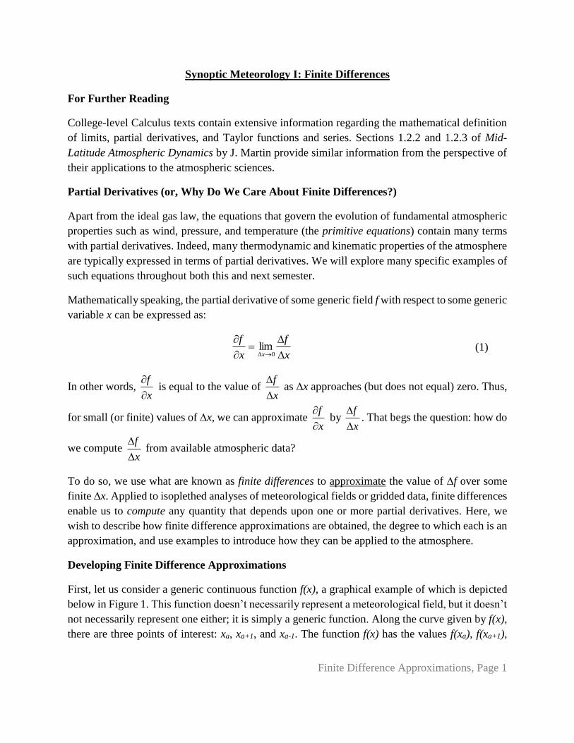
College-level Calculus texts contain extensive information regarding the mathematical definition
of limits, partial derivatives, and Taylor functions and series. Sections 1.2.2 and 1.2.3 of Mid-
Latitude Atmospheric Dynamics by J. Martin provide similar information from the perspective of
their applications to the atmospheric sciences.
Partial Derivatives (or, Why Do We Care About Finite Differences?)
Apart from the ideal gas law, the equations that govern the evolution of fundamental atmospheric
properties such as wind, pressure, and temperature (the primitive equations) contain many terms
with partial derivatives. Indeed, many thermodynamic and kinematic properties of the atmosphere
are typically expressed in terms of partial derivatives. We will explore many specific examples of
such equations throughout both this and next semester.
Mathematically speaking, the partial derivative of some generic field f with respect to some generic
variable x can be expressed as:
x
f
x
f
x
0lim (1)
In other words, x
f
is equal to the value of
x
f
as ∆x approaches (but does not equal) zero. Thus,
for small (or finite) values of ∆x, we can approximate x
f
by
x
f
. That begs the question: how do
we compute x
f
from available atmospheric data?
To do so, we use what are known as finite differences to approximate the value of ∆f over some
finite ∆x. Applied to isoplethed analyses of meteorological fields or gridded data, finite differences
enable us to compute any quantity that depends upon one or more partial derivatives. Here, we
wish to describe how finite difference approximations are obtained, the degree to which each is an
approximation, and use examples to introduce how they can be applied to the atmosphere.
Developing Finite Difference Approximations
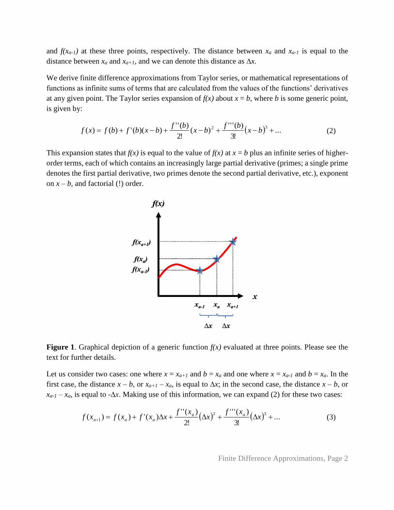
First, let us consider a generic continuous function f(x), a graphical example of which is depicted
below in Figure 1. This function doesn’t necessarily represent a meteorological field, but it doesn’t
not necessarily represent one either; it is simply a generic function. Along the curve given by f(x),
there are three points of interest: xa, xa+1, and xa-1. The function f(x) has the values f(xa), f(xa+1),
Finite Difference Approximations, Page 2
and f(xa-1) at these three points, respectively. The distance between xa and xa-1 is equal to the
distance between xa and xa+1, and we can denote this distance as ∆x.
We derive finite difference approximations from Taylor series, or mathematical representations of
functions as infinite sums of terms that are calculated from the values of the functions’ derivatives
at any given point. The Taylor series expansion of f(x) about x = b, where b is some generic point,
is given by:
...!3
)(''')(
!2
)(''))((')()(
32 bxbf
bxbf
bxbfbfxf (2)
This expansion states that f(x) is equal to the value of f(x) at x = b plus an infinite series of higher-
order terms, each of which contains an increasingly large partial derivative (primes; a single prime
denotes the first partial derivative, two primes denote the second partial derivative, etc.), exponent
on x – b, and factorial (!) order.
Figure 1. Graphical depiction of a generic function f(x) evaluated at three points. Please see the
text for further details.
Let us consider two cases: one where x = xa+1 and b = xa and one where x = xa-1 and b = xa. In the
first case, the distance x – b, or xa+1 – xa, is equal to ∆x; in the second case, the distance x – b, or
xa-1 – xa, is equal to -∆x. Making use of this information, we can expand (2) for these two cases:
...!3
)('''
!2
)('')(')()(
32
1 xxf
xxf
xxfxfxf aa
aaa (3)
Finite Difference Approximations, Page 3
...!3
)('''
!2
)('')(')()(
32
1 xxf
xxf
xxfxfxf aa
aaa (4)
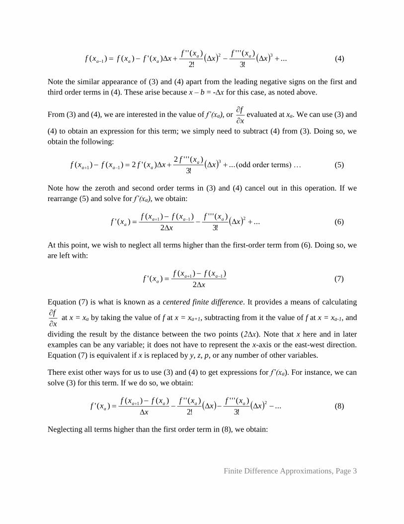
Note the similar appearance of (3) and (4) apart from the leading negative signs on the first and
third order terms in (4). These arise because x – b = -∆x for this case, as noted above.
From (3) and (4), we are interested in the value of f’(xa), or x
f
evaluated at xa. We can use (3) and
(4) to obtain an expression for this term; we simply need to subtract (4) from (3). Doing so, we
obtain the following:
...!3
)('''2)('2)()(
3
11 xxf
xxfxfxf a
aaa (odd order terms) … (5)
Note how the zeroth and second order terms in (3) and (4) cancel out in this operation. If we
rearrange (5) and solve for f’(xa), we obtain:
...!3
)('''
2
)()()('
211
x
xf
x
xfxfxf aaa
a (6)
At this point, we wish to neglect all terms higher than the first-order term from (6). Doing so, we
are left with:
x
xfxfxf aa
a
2
)()()(' 11 (7)
Equation (7) is what is known as a centered finite difference. It provides a means of calculating
x
f
at x = xa by taking the value of f at x = xa+1, subtracting from it the value of f at x = xa-1, and
dividing the result by the distance between the two points (2∆x). Note that x here and in later
examples can be any variable; it does not have to represent the x-axis or the east-west direction.
Equation (7) is equivalent if x is replaced by y, z, p, or any number of other variables.
There exist other ways for us to use (3) and (4) to get expressions for f’(xa). For instance, we can
solve (3) for this term. If we do so, we obtain:
...!3
)('''
!2
)('')()()('
21
x
xfx
xf
x
xfxfxf aaaa
a (8)
Neglecting all terms higher than the first order term in (8), we obtain:
Finite Difference Approximations, Page 4
x
xfxfxf aa
a
)()(
)(' 1 (9)
Equation (9) is what is known as a forward finite difference. It provides a means of calculating x
f
at x = xa by taking the value of f at x = xa+1, subtracting from it the value of f at x = xa, and dividing
the result by the distance between the two points (∆x).
Alternatively, we can solve (4) for f’(xa). If we do so, we obtain:
...!3
)('''
!2
)('')()()('
21
x
xfx
xf
x
xfxfxf aaaa
a (10)
Neglecting all terms higher than the first order term in (10), we obtain:
x
xfxfxf aa
a
)()(
)(' 1 (11)
Equation (11) is what is known as a backward finite difference. It provides a means of calculating
x
f
at x = xa by taking the value of f at x = xa, subtracting from it the value of f at x = xa-1, and
dividing the result by the distance between the two points (∆x).
Finite Differences as Approximations
We do not need to neglect the higher-order terms in obtaining any of the above expressions for
f’(xa); we have done so here primarily for simplicity. If we were to retain the higher-order terms,
we would obtain more accurate approximations for f’(xa). This highlights a key point: all finite
differences are approximations. All finite differences are associated with what is known as
truncation error, which is determined by the power of ∆x on the first term that is neglected in
obtaining the finite difference approximation.
For instance, consider our centered finite difference given by Equation (7). In obtaining (7), the
first term that we neglected in (6) included a (∆x)2 term. As a result, we say this finite difference
is “second-order–accurate.” In contrast, consider our forward and backward finite differences,
given by Equations (9) and (11), respectively. In obtaining each equation, the first terms that we
neglected in (8) and (10) included a (∆x) term. As a result, we say that these finite differences are
“first-order–accurate.” The higher the order of accuracy, the more accurate the finite difference.
In synoptic meteorology, where exact values for partial derivatives are often not necessary, we
typically utilize the centered finite difference. Forward and backward finite differences are rarely
utilized except along the edges of the data, where the -1 and +1 points may not exist. Higher-order
finite differences, typically fourth- or higher-order–accurate, are necessary for numerical weather
Finite Difference Approximations, Page 5
prediction models given chaos theory, which states that very small differences in data can lead to
very large forecast differences.
A Finite Difference Approximation for Second Derivatives
While the first partial derivative of some field provides a measure of its slope, sometimes we are
interested in evaluating the second partial derivative of some field. Recall from calculus that the
second partial derivative of a field provides a measure of its concavity; positive second partial
derivatives infer that a field is concave up (or convex), while negative second partial derivatives
infer that a field is concave down. Applied to meteorology, a field that is convex represents a local
minimum, whereas a field that is concave down represents a local maximum; i.e., the second partial
derivative has the opposite sign of the field itself.
We can obtain a finite difference approximation for the second partial derivative by adding (3) and
(4). Doing so, we obtain:
...!2
)(''2)(2)()(
2
11 xxf
xfxfxf a
aaa (12)
If we solve (12) for f’’(xa) and truncate the higher-order terms, we obtain:
2
11 )(2)()()(''
x
xfxfxfxf aaa
a
(13)
Equation (13) provides a fourth-order–accurate means of evaluating 2
2
x
f
, or )('' axf , by adding
the value of f at xa+1 to the value of f at xa-1, subtracting two times the value of f at xa, and dividing
the result by the square of the distance between points (∆x)2.
Just as for the finite difference approximation for the first partial derivative, (13) is equivalent if x
is replaced by y, z, p, or any number of other variables. Likewise, just as for the finite difference
approximate for the first partial derivative, higher-order accurate finite difference approximations
for the second partial derivative can also be obtained.
Applying Finite Differences: Advection Examples
One of the most important attributes of the wind is its ability to transport. The transport of some
quantity by the wind is known as advection. We are most often interested in its horizontal transport,
or horizontal advection, where the horizontal surface can be taken to be Earth’s surface, a constant
height surface, an isobaric surface, or even an isentropic surface. For convenience, we sometimes
refer to horizontal advection simply as advection.
Finite Difference Approximations, Page 6
In synoptic meteorology, we are particularly interested in temperature advection, referring to the
horizontal transport of energy (recall that temperature is simply a measure of the average kinetic
energy of the air) by the wind. Patterns of cold air advection and warm air advection reflect the
(horizontal) motion of air masses and, as we will see next semester, play a crucial role in forcing
vertical motions, can bring about changes in the amplitude of troughs and ridges, and can influence
cyclone and anticyclone development.
Mathematically, temperature advection is expressed as the product of the appropriate component
of the wind – whether east-west (u; also known as the zonal wind component) or north-south (v;
also known as the meridional wind component) – and the local change of temperature in some
direction – east-west (x) or north-south (y) – where:
y
Tv
x
Tuadvection
(14)
In vector notation, (14) can be written as:
Tadvection v
(15)
The units of temperature advection are the units of wind – m s-1 – multiplied by the units of
temperature – generally either °C or K – divided by distance units – m. As a result, temperature
advection has units of °C s-1 or K s-1; in other words, how temperature is changing locally over
some finite amount of time ∆t. We can evaluate (14) from charts of weather data using our centered
finite difference approximation developed above.
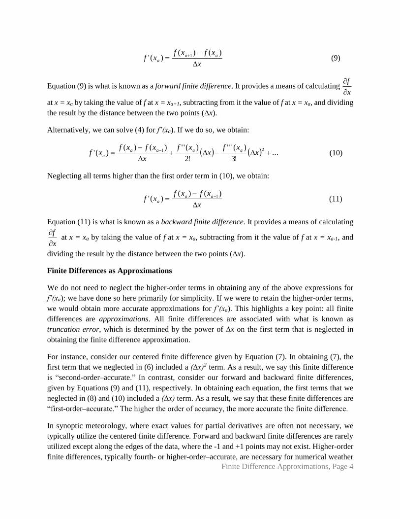
Consider the hypothetical analysis presented in Figure 2. We are interested in computing the
horizontal temperature advection at the point marked by the closed circle and wind observation.
We have already completed an isotherm analysis using temperature data from this point as well as
the other locations that surround it. We thus have everything we need for our calculation.
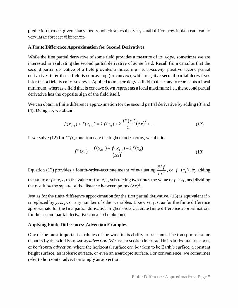
To compute horizontal temperature advection, we must first set up our x- and y-axes. Fortunately,
since we are told in the Figure 2 caption that the data are plotted on a Mercator map projection,
the positive x-axis points to the right, or due east, while the positive y-axis points up, or due north.
Since our centered finite difference approximation is only valid over finite distances – here, ∆x
and ∆y – we must set up a small, uniform grid centered on the wind observation location. This is
done so that we can estimate the temperature at points x+1, x-1, y+1, and y-1 – in other words, the
terms that enter the numerator of our centered finite differences. The result of doing so is given in
Figure 3.
Finite Difference Approximations, Page 7
Figure 2. Hypothetical surface temperature observations (°F, red numbers), isotherm analysis
(every 5°F, black lines), and a single wind observation (10 kt = 5.15 m s-1 out of the northwest).
Depicted for reference are horizontal scales and the north and east cardinal directions. Data are
plotted on a map constructed using the Mercator map projection.
Figure 3. As in Figure 2, except with a finite grid drawn in centered on our wind observation. Both
in this example and in practice, the distance ∆x is taken to be equal to the distance ∆y. In this case,
using the distance references on the edges of the map, both ∆x and ∆y are 50 km (or 50,000 m).
Finite Difference Approximations, Page 8
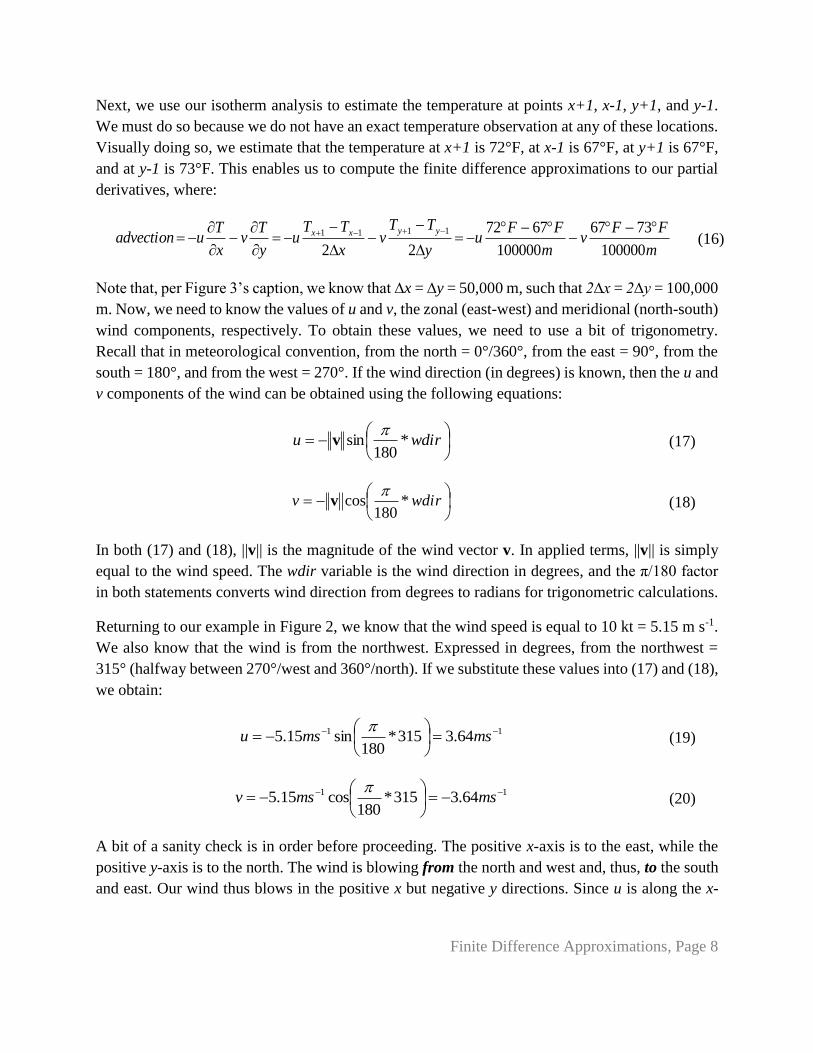
Next, we use our isotherm analysis to estimate the temperature at points x+1, x-1, y+1, and y-1.
We must do so because we do not have an exact temperature observation at any of these locations.
Visually doing so, we estimate that the temperature at x+1 is 72°F, at x-1 is 67°F, at y+1 is 67°F,
and at y-1 is 73°F. This enables us to compute the finite difference approximations to our partial
derivatives, where:
m
FFv
m
FFu
y
TTv
x
TTu
y
Tv
x
Tuadvection
yyxx
100000
7367
100000
6772
22
1111
(16)
Note that, per Figure 3’s caption, we know that ∆x = ∆y = 50,000 m, such that 2∆x = 2∆y = 100,000
m. Now, we need to know the values of u and v, the zonal (east-west) and meridional (north-south)
wind components, respectively. To obtain these values, we need to use a bit of trigonometry.
Recall that in meteorological convention, from the north = 0°/360°, from the east = 90°, from the
south = 180°, and from the west = 270°. If the wind direction (in degrees) is known, then the u and
v components of the wind can be obtained using the following equations:
wdiru *
180sin
v (17)
wdirv *
180cos
v (18)
In both (17) and (18), ||v|| is the magnitude of the wind vector v. In applied terms, ||v|| is simply
equal to the wind speed. The wdir variable is the wind direction in degrees, and the π/180 factor
in both statements converts wind direction from degrees to radians for trigonometric calculations.
Returning to our example in Figure 2, we know that the wind speed is equal to 10 kt = 5.15 m s-1.
We also know that the wind is from the northwest. Expressed in degrees, from the northwest =
315° (halfway between 270°/west and 360°/north). If we substitute these values into (17) and (18),
we obtain:
11 64.3315*180
sin15.5
msmsu
(19)
11 64.3315*180
cos15.5
msmsv
(20)
A bit of a sanity check is in order before proceeding. The positive x-axis is to the east, while the
positive y-axis is to the north. The wind is blowing from the north and west and, thus, to the south
and east. Our wind thus blows in the positive x but negative y directions. Since u is along the x-
Finite Difference Approximations, Page 9
axis (east-west) and v is along the y-axis (north-south), we would expect that u should be positive
and v should be negative for a northwest wind – and, indeed, we find that this is true.
If we plug (19) and (20) into (16) and run through the calculations, we obtain:
111 0004.0100000
736764.3
100000
677264.3
Fs
m
FFms
m
FFmsadvection (21)
In other words, due solely to horizontal advection, the temperature at the location of our wind
observation is cooling by 0.0004°F every second. If we multiply this by 3,600 (the number of
seconds in one hour) or 84,600 (the number of seconds in one day), we can convert this to °F h-1
or °F day-1, respectively. Doing so, we obtain values of -1.44°F h-1 and -34.56°F day-1. In other
words, due solely to horizontal advection, the temperature at the location of our wind observation
is cooling by 1.44°F every hour and 34.56°F every day. Of course, horizontal advection is far from
the only thing controlling the temperature at a given location – for instance, changes in cloud cover
or time of day exert a significant influence on temperature – such that the estimated temperature
change due to advection is usually much larger than the actual temperature change.
Before we proceed further, it is again time for another sanity check. In Figure 2, we see that the
wind is blowing toward the station from where it is colder. As a result, we would expect the wind
to be advecting (or transporting) colder air toward the observation station. Our calculation suggests
that this is true – due to advection, the temperature at the observation station is cooling.
The above calculation process is a complex means of evaluating horizontal temperature advection.
By contrast, our sanity check hints at another, far less complex means of doing so. Instead of using
Cartesian (x,y) coordinates, as we did before, we may use a natural coordinate system to assess
horizontal temperature advection.
Recall that in the natural coordinate system, the appropriate coordinates become s, or along
(streamwise) the wind, and n, or normal to the wind. For the example given in Figure 2, the
positive s-axis points to the southeast, in the direction that the wind is blowing, and the positive n-
axis points to the northeast, or 90° to the left of the positive s-axis. Figure 4 below provides a
graphical depiction of the natural coordinate system applied to the example from Figures 2 and 3.
Finite Difference Approximations, Page 10
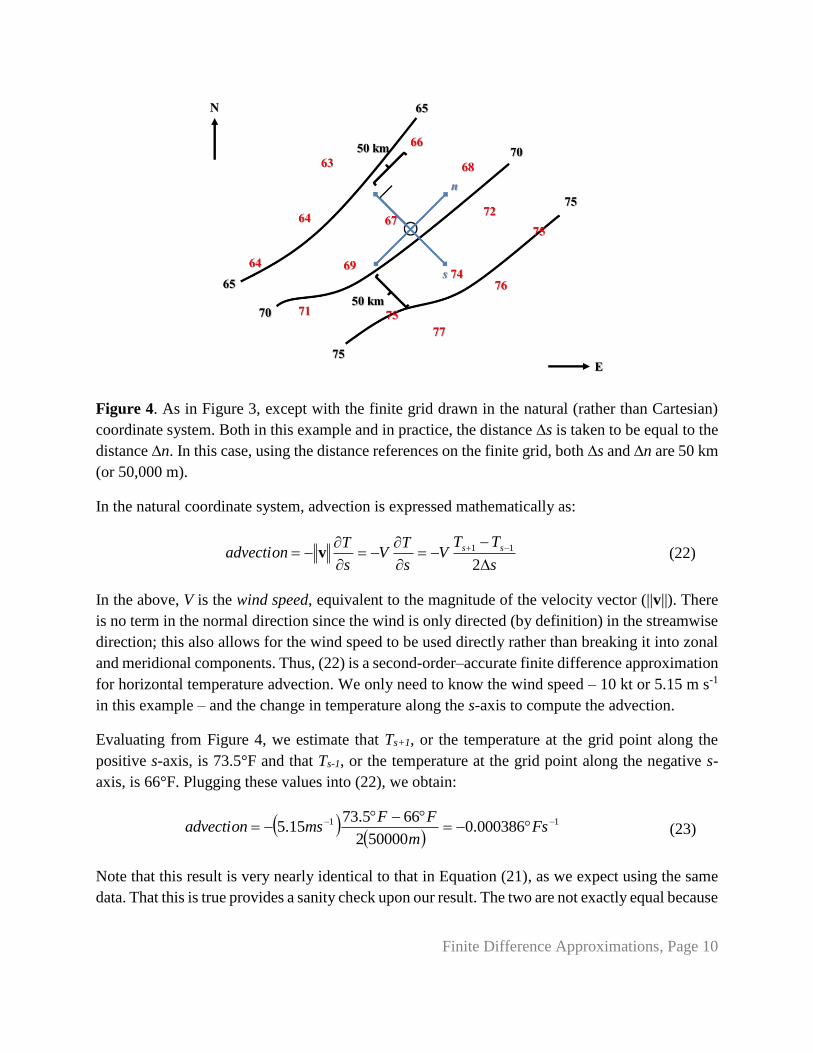
Figure 4. As in Figure 3, except with the finite grid drawn in the natural (rather than Cartesian)
coordinate system. Both in this example and in practice, the distance ∆s is taken to be equal to the
distance ∆n. In this case, using the distance references on the finite grid, both ∆s and ∆n are 50 km
(or 50,000 m).
In the natural coordinate system, advection is expressed mathematically as:
s
TTV
s
TV
s
Tadvection ss
2
11v (22)
In the above, V is the wind speed, equivalent to the magnitude of the velocity vector (||v||). There
is no term in the normal direction since the wind is only directed (by definition) in the streamwise
direction; this also allows for the wind speed to be used directly rather than breaking it into zonal
and meridional components. Thus, (22) is a second-order–accurate finite difference approximation
for horizontal temperature advection. We only need to know the wind speed – 10 kt or 5.15 m s-1
in this example – and the change in temperature along the s-axis to compute the advection.
Evaluating from Figure 4, we estimate that Ts+1, or the temperature at the grid point along the
positive s-axis, is 73.5°F and that Ts-1, or the temperature at the grid point along the negative s-
axis, is 66°F. Plugging these values into (22), we obtain:
11 000386.0500002
665.7315.5
Fs
m
FFmsadvection (23)
Note that this result is very nearly identical to that in Equation (21), as we expect using the same
data. That this is true provides a sanity check upon our result. The two are not exactly equal because
Finite Difference Approximations, Page 11
of the inherent approximate nature to each of our two analyses, namely in obtaining the values of
T at each of our grid points.
Though this example only demonstrates two ways of computing horizontal temperature advection
for a single set of data, we can nevertheless build on the concepts developed through the example
to state several general rules for temperature advection in specific and advection more generally:
• Cold air advection occurs when the wind blows from cold toward warm air. Conversely,
warm air advection occurs when the wind blows from warm toward cold air. In the general
case, negative advection occurs when the wind blows from smaller toward larger values,
whereas positive advection occurs when the wind blows from larger toward smaller values.
• When the change in advected quantity over a fixed distance is large, the magnitude of the
advection is large. When the change in advected quantity over a fixed distance is small, the
magnitude of the advection is small. For example, if the temperature at the s+1 and s-1
points in Figure 4 were 77.5°F and 62°F, respectively, instead of 73.5°F and 66°F, then the
change in temperature over the 2Δs interval would be 15.5°F and the advection would be
-0.000798°F s-1.
• When the wind is parallel to the isolines, no horizontal advection occurs. For example, if
the wind in Figure 4 were from the southwest instead of from the northwest, the
temperature at the s+1 and s-1 points would both be 68°F, and the advection would be 0°F
s-1. Conversely, when the wind is perpendicular to the isotherms/isohypses, horizontal
advection is maximized. This is true for the examples in Figures 3 and 4.
• When the wind component blowing perpendicular to the isolines is larger, horizontal
advection is larger. For example, if the wind in Figure 4 were 20 kt (10.3 m s-1) instead of
10 kt (5.15 m s-1), the advection would be doubled (-0.000773°F s-1). Conversely, when
the wind component blowing perpendicular to the isolines is smaller, horizontal advection
is smaller.
Let us now demonstrate a qualitative application of these rules to horizontal temperature advection,
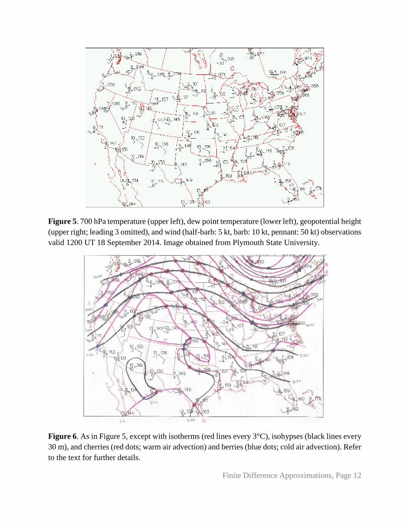
colloquially known as “cherries and berries.” Consider the 700 hPa observations, including wind
and temperature, given in Figure 5. We can use our principles of isoplething to create a temperature
(isotherm) and geopotential height (isohypse) analysis, as is depicted in Figure 6. In Figure 6, we
can see that the wind generally blows parallel to the isohypses, with lower geopotential heights to
the left of the wind. This information allows us to conduct our “cherries and berries” analysis at
each intersection of an isohypse with an isotherm, and the result of doing so is given by the blue
(for cold air advection) and red (for warm air advection) dots on Figure 6.
Finite Difference Approximations, Page 12
Figure 5. 700 hPa temperature (upper left), dew point temperature (lower left), geopotential height
(upper right; leading 3 omitted), and wind (half-barb: 5 kt, barb: 10 kt, pennant: 50 kt) observations
valid 1200 UT 18 September 2014. Image obtained from Plymouth State University.
Figure 6. As in Figure 5, except with isotherms (red lines every 3°C), isohypses (black lines every
30 m), and cherries (red dots; warm air advection) and berries (blue dots; cold air advection). Refer
to the text for further details.

Finite Difference Approximations, Page 13
In Figure 6, note that the cherries and berries are not random but instead are organized in a distinct
pattern: primarily cold air advection along the west and east coasts, primarily warm air advection
in the central United States. Dots are more densely packed where the isotherms and/or isohypses
are more densely packed, representing regions in which temperature changes are large over a small
horizontal distance and where the wind speed is large, respectively; in this sense, dot density gives
an estimate of the advection magnitude (larger where more densely packed, smaller where less so).
A Refresher on Vector Notation
As partial derivatives are found in nearly all aspects of synoptic meteorology, it is useful to close
by reminding ourselves of some of their basic properties, particularly as it relates to vectors. In the
last section, we noted that horizontal temperature advection can be written as:
T Tadvection u v T
x y
v (24)
The first representation is written in what is known as component notation, whereas the second is
in what is known as vector notation (here, assuming that the gradient operator applies only in the
horizontal direction). The two are equivalent to each other because of the definitions of the gradient
operator and dot product, i.e.,
x y
i j x y x y x x y ya a b b a b a b a b i j i j
where we have again considered only the horizontal directions in this analysis. For the dot product,
a is simply u v v i j and b is simply T T
x y
i j .
There are other quantities that can be written in component or vector notation that we will consider
in more detail later in the semester. For example, consider the divergence of the horizontal wind:
u vdivergence
x y
v (25)
This is a relatively straightforward application of the gradient operator and dot product, the proof
of which is left to the student. We can also consider the vertical component of the vorticity of the
horizontal wind:
v u
vorticityx y
k v (26)
Finite Difference Approximations, Page 14
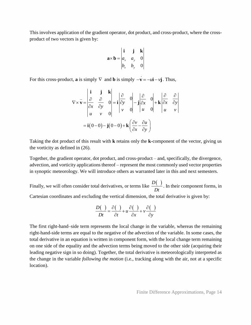
This involves application of the gradient operator, dot product, and cross-product, where the cross-
product of two vectors is given by:
0
0
x y
x y
a a
b b
i j k
a b
For this cross-product, a is simply and b is simply u v v i j . Thus,
0 00
000
0 0 0 0
y x yxx y
uv u vu v
v u
x y
i j k
v i j k
i j k
Taking the dot product of this result with k retains only the k-component of the vector, giving us
the vorticity as defined in (26).
Together, the gradient operator, dot product, and cross-product – and, specifically, the divergence,
advection, and vorticity applications thereof – represent the most commonly used vector properties
in synoptic meteorology. We will introduce others as warranted later in this and next semesters.
Finally, we will often consider total derivatives, or terms like D
Dt. In their component forms, in
Cartesian coordinates and excluding the vertical dimension, the total derivative is given by:
Du v
Dt t x y
The first right-hand–side term represents the local change in the variable, whereas the remaining
right-hand-side terms are equal to the negative of the advection of the variable. In some cases, the
total derivative in an equation is written in component form, with the local change term remaining
on one side of the equality and the advection terms being moved to the other side (acquiring their
leading negative sign in so doing). Together, the total derivative is meteorologically interpreted as
the change in the variable following the motion (i.e., tracking along with the air, not at a specific
location).