Embed Size (px)
Citation preview
2SYSTEM DYNAMICS PROBLEMS WITH RATE PROPORTIONAL TO AMOUNT
In order to view this proof accurately, the Overprint Preview Option must be checked in Acrobat Professional or Adobe Reader. Please contact your Customer Service Rep-
resentative if you have questions about finding the option.
Job Name: Cyan = PMS 300/356585t
© Copyright, Princeton University Press. No part of this book may be distributed, posted, or reproduced in any form by digital or mechanical means without prior written permission of the publisher.

MODULE 2.1
System Dynamics Tool—Tutorial 1
Download
From the textbook’s website, download Tutorial 1 in PDF format for your system dynamics tool. We recommend that you work through the tutorial and answer all Quick Review Questions using the corresponding software.
Introduction
Dynamic systems, which change with time, are usually very complex, having many components, with involved relationships. Two examples are systems involving com-petition among different species for limited resources and the kinetics of enzymatic reactions.
With a system dynamics tool, we can model complex systems using diagrams and equations. Thus, such a tool helps us perform Step 2 of the modeling process—for-mulate a model—by helping us document our simplifying assumptions, variables, and units; establish relationships among variables and submodels; and record equa-tions and functions. Then, a system dynamics tool can help us solve the model—Step 3 of the modeling process—by performing simulations using the model and generating tables and graphs of the results. We use this output to perform Step 4 of the modeling process—verify and interpret the model’s solution. Often such exami-nation leads us to change a model. With its graphical view and built-in functions, a system dynamics tool facilitates cycling back to an earlier step of the modeling pro-cess to simplify or refine a model. Once we have verified and validated a model, the tool’s diagrams and equations from the design and the results from the simulation should be part of our report, which we do in Step 5 of the modeling process. The tool can even help us as we maintain the model (Step 6) by making corrections, improve-ments, or enhancements.
In order to view this proof accurately, the Overprint Preview Option must be checked in Acrobat Professional or Adobe Reader. Please contact your Customer Service Rep-
resentative if you have questions about finding the option.
Job Name: Cyan = PMS 300/356585t
© Copyright, Princeton University Press. No part of this book may be distributed, posted, or reproduced in any form by digital or mechanical means without prior written permission of the publisher.

16 Module 2.1
This first tutorial is available for download from the textbook’s website for sev-eral different system dynamics tools. Tutorial 1 in your system of choice prepares you to perform basic modeling with such a tool, including the following:
• Diagramming a model• Entering equations and values• Running a simulation• Constructing graphs • Producing tables
The module gives examples and Quick Review Questions for you to complete and execute with your desired tool.
In order to view this proof accurately, the Overprint Preview Option must be checked in Acrobat Professional or Adobe Reader. Please contact your Customer Service Rep-
resentative if you have questions about finding the option.
Job Name: Cyan = PMS 300/356585t
© Copyright, Princeton University Press. No part of this book may be distributed, posted, or reproduced in any form by digital or mechanical means without prior written permission of the publisher.
MODULE 2.2
Unconstrained Growth and Decay
Introduction
Many situations exist where the rate at which an amount is changing is proportional to the amount present. Such might be the case for a population of people, deer, or bacteria, for example. When money is compounded continuously, the rate of change of the amount is also proportional to the amount present. For a radioactive element, the amount of radioactivity decays at a rate proportional to the amount present. Simi-larly, the concentration of a chemical pollutant decays at a rate proportional to the concentration of pollutant present.
Rate of Change
We deal with rate of change every time we drive a car. Suppose our position (y) is a function (s) of time (t), so we write y = s(t). Suppose also that we start driving on a straight road at time t = 0 hours (h) at position marker s(0) = 10 miles (mi; about 16.1 km), and at time t = 2 h we are at position s(2) = 116 mi (about 186.7 km). Our average velocity, or average rate of change of position with respect to time, is the change in position (∆s) over the change in time (∆ t) and incorporates average speed as well as direction by its sign:
average velocity = ∆∆st
= 116 106 53 mi 10 mi2 h 0 h
mi2 h
mi/h−−
= =
or
average velocity = ∆∆st
= 186 7 170 6 85 3. . . km 16.1 km2 h 0 h
km2 h
km/h−−
= =
We probably are not driving at a constant rate of 53 mi/h (85.3 km/h), but sometimes we are moving faster and other times, slower. To obtain a more accurate measure of
In order to view this proof accurately, the Overprint Preview Option must be checked in Acrobat Professional or Adobe Reader. Please contact your Customer Service Rep-
resentative if you have questions about finding the option.
Job Name: Cyan = PMS 300/356585t
© Copyright, Princeton University Press. No part of this book may be distributed, posted, or reproduced in any form by digital or mechanical means without prior written permission of the publisher.
18 Module 2.2
our velocity at time t = 1 h, we can use a smaller interval. For instance, at time t = 1 h, our position might be at marker s(1) = 51.2 mi, while a short time before at t = 0.98 h, our position was s(0.98) = 50.0 mi. As the following calculation shows, over this interval of 0.02 h (1.2 min), our average velocity is faster, 60 mi/h:
average velocity = ∆∆st
= 51 2 1 2 60. . mi 50 mi1.00 h 0.98 h
mi0.02 h
mi/h−−
= =
or about 96.6 km/h.
Quick Review Question 1
Suppose on a windless day someone standing on a bridge holds a ball over the side and tosses the ball straight up into the air. After reaching its highest point, the ball falls, eventually landing in the water. The ball’s height in meters (m) above the water (y) is a function (s) of time (t) in seconds (s), or y = s(t).
a. Determine the average velocity with units of the ball from t = 1 s to t = 2 s if s(1) = 21.1 m and s(2) = 21.4 m.
b. Determine the average velocity with units of the ball from t = 1 s to t = 3 s if s(1) = 21.1 m and s(3) = 11.9 m.
c. Using the notation of the definition of average velocity, for Part b determine the following, including units: b, s(b), ∆t, b – ∆t, s(b – ∆t), ∆s.
By making the interval smaller and smaller around the time t = 1 h, the average velocity calculation approaches our precise velocity at t = 1 h, or our instantaneous rate of change of position with respect to time, which is our odometer’s reading. This instantaneous rate of change of s with respect to t is the derivative of s with
respect to t, written as sʹ(t), or dydt
, or dy/dt; and sʹ(1), or dsdt t=1
, indicates the deriva-tive at time t = 1 h.
Definition Suppose s(t) is the position of an object at time t, where a ≤ t ≤ b. Then the change in time, ∆t, is ∆t = b – a; and the change in position, ∆s, is ∆s = s(b) – s(a). Moreover, the aver-age velocity, or the average rate of change of s with respect to t, of the object from time a = b – ∆t to time b is
average velocity change in positionchange in time
(= = =∆∆sts b)) ( )−
−= − −s a
b as b s b t
t( ) ( )∆
∆
average velocity change in positionchange in time
(= = =∆∆sts b)) ( )−
−= − −s a
b as b s b t
t( ) ( )∆
∆
In order to view this proof accurately, the Overprint Preview Option must be checked in Acrobat Professional or Adobe Reader. Please contact your Customer Service Rep-
resentative if you have questions about finding the option.
Job Name: Cyan = PMS 300/356585t
© Copyright, Princeton University Press. No part of this book may be distributed, posted, or reproduced in any form by digital or mechanical means without prior written permission of the publisher.
System Dynamics Problems with Rate Proportional to Amount 19
A function, such as y = s(t), can represent many things other than position. More-over, we are not restricted to using symbols, such as s. For example, Q(t) might represent a quantity (mass) of radioactive carbon-14 at time t, and the instantaneous rate of change of Q with respect to t, Qʹ(t) = dQ/dt, is the instantaneous rate of decay. As another example, P(t) might symbolize a population at time t, so that Pʹ(t) = dP/dt, is the rate of change of the population with respect to t.
Differential Equation
Continuing with the population example, suppose we have a population in which no individuals arrive or depart; the only change in the population comes from births and deaths. No constraints, such as competition for food or a predator, exist on growth of the population. When no limiting factor exists, we have the Malthusian model for unconstrained population growth, where the rate of change of the population is di-rectly proportional (∝) to the number of individuals in the population. If P repre-sents the population and t represents time, then we have the following proportion:
dPdt
P∝
For a positive growth rate, the larger the population, the greater the change in the population. With the same positive growth rate in two cities, say New York City and Spartanburg, S.C., the population of the larger New York City increases more in magnitude in a year than that of Spartanburg. In a later section of this module, “Un-constrained Decay,” we consider a situation in which the rate is negative.
We write the preceding proportion in equation form as follows:
dPdt
rP=
The constant r is the growth rate, or instantaneous growth rate, or continuous growth rate, while dP/dt is the rate of change of the population.
Definition The instantaneous velocity, or the instantaneous rate of change of s with respect to t, at t = b is the number the average
velocity, s b s b tt
( ) ( )− − ∆∆
, approaches as ∆t comes closer and
closer to 0 (provided the ratio approaches a number). In this case, the derivative of y = s(t) with respect to t at t = b, written sʹ(b)
or dydt t b=
, is the instantaneous velocity at t = b. In general, the
derivative of y = s(t) with respect to t is written as sʹ(t), or dydt
, or dy/dt.
In order to view this proof accurately, the Overprint Preview Option must be checked in Acrobat Professional or Adobe Reader. Please contact your Customer Service Rep-
resentative if you have questions about finding the option.
Job Name: Cyan = PMS 300/356585t
© Copyright, Princeton University Press. No part of this book may be distributed, posted, or reproduced in any form by digital or mechanical means without prior written permission of the publisher.
20 Module 2.2
In “System Dynamics Tool—Tutorial 1” (Module 2.1), we started with a bacte-rial population of size 100, an instantaneous growth rate of 10% = 0.10, and time measured in hours. Thus, we had
dPdt
P= 0 10.
with P0 = 100. The equation dPdt
P= 0 10. with the initial condition P0 = 100 is a
differential equation because it contains a derivative. A solution to this differential equation is a function, P(t), whose derivative is 0.10P(t), with P(0) = 100. We begin by reconsidering this example from Tutorial 1 for reinforcement and a more in-depth examination of the concepts.
Difference Equation
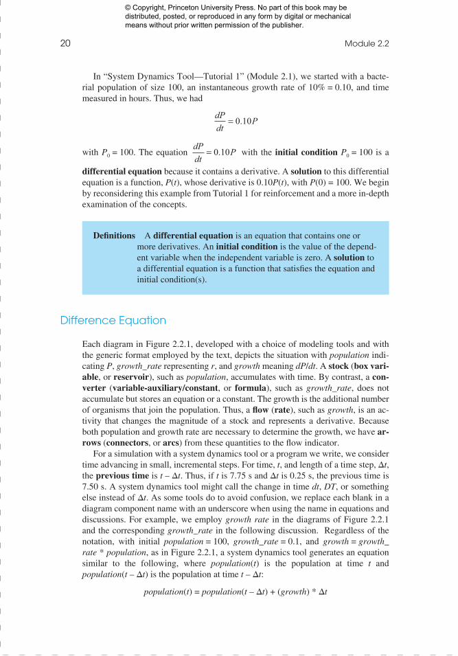
Each diagram in Figure 2.2.1, developed with a choice of modeling tools and with the generic format employed by the text, depicts the situation with population indi-cating P, growth_rate representing r, and growth meaning dP/dt. A stock (box vari-able, or reservoir), such as population, accumulates with time. By contrast, a con-verter (variable-auxiliary/constant, or formula), such as growth_rate, does not accumulate but stores an equation or a constant. The growth is the additional number of organisms that join the population. Thus, a flow (rate), such as growth, is an ac-tivity that changes the magnitude of a stock and represents a derivative. Because both population and growth rate are necessary to determine the growth, we have ar-rows (connectors, or arcs) from these quantities to the flow indicator.
For a simulation with a system dynamics tool or a program we write, we consider time advancing in small, incremental steps. For time, t, and length of a time step, ∆t, the previous time is t – ∆t. Thus, if t is 7.75 s and ∆t is 0.25 s, the previous time is 7.50 s. A system dynamics tool might call the change in time dt, DT, or something else instead of ∆t. As some tools do to avoid confusion, we replace each blank in a diagram component name with an underscore when using the name in equations and discussions. For example, we employ growth rate in the diagrams of Figure 2.2.1 and the corresponding growth_rate in the following discussion. Regardless of the notation, with initial population = 100, growth_rate = 0.1, and growth = growth_rate * population, as in Figure 2.2.1, a system dynamics tool generates an equation similar to the following, where population(t) is the population at time t and population(t – ∆t) is the population at time t – ∆t:
population(t) = population(t – ∆t) + (growth) * ∆t
Definitions A differential equation is an equation that contains one or more derivatives. An initial condition is the value of the depend-ent variable when the independent variable is zero. A solution to a differential equation is a function that satisfies the equation and initial condition(s).
In order to view this proof accurately, the Overprint Preview Option must be checked in Acrobat Professional or Adobe Reader. Please contact your Customer Service Rep-
resentative if you have questions about finding the option.
Job Name: Cyan = PMS 300/356585t
© Copyright, Princeton University Press. No part of this book may be distributed, posted, or reproduced in any form by digital or mechanical means without prior written permission of the publisher.
System Dynamics Problems with Rate Proportional to Amount 21
This equation, called a finite difference equation, indicates that the population at one time step is the population at the previous time step plus the change in popula-tion over that time interval:
(new population) = (old population) + (change in population)
or
population(t) = population(t – ∆t) + ∆population
where ∆population is a notation for the change in population. We approximate the change in the population over one time step, ∆population or (growth) * ∆t, as the finite difference of the populations at one time step and at the previous time step, population(t) – population(t – ∆t). Thus, solving for growth, we have an approxima-tion of the derivative dP/dt as follows:
growth = ∆∆
∆∆
populationt
population t population t tt
= − −( ) ( )
Computer programs and system dynamics tools employ such finite difference equa-tions to solve differential equations.
population
growth
growth rate
populationgrowth
growth rate growth rate
growthpopulation
a b
c d
growth
growth rate
population
•
Figure 2.2.1 Diagrams of population models where growth rate is proportional to popula-tion: (a) Berkeley Madonna® (b) STELLA® (c) Vensim PLE® (d) Text’s format
In order to view this proof accurately, the Overprint Preview Option must be checked in Acrobat Professional or Adobe Reader. Please contact your Customer Service Rep-
resentative if you have questions about finding the option.
Job Name: Cyan = PMS 300/356585t
© Copyright, Princeton University Press. No part of this book may be distributed, posted, or reproduced in any form by digital or mechanical means without prior written permission of the publisher.
22 Module 2.2
Quick Review Question 2
Consider the differential equation dQ/dt = – 0.0004Q, with Q0 = 200.
a. Using delta notation, give a finite difference equation corresponding to the differential equation.
b. At time t = 9.0 s, give the time at the previous time step, where ∆t = 0.5 s.c. If Q(t – ∆t) = 199.32 and Q(t) = 199.28, give ∆Q.
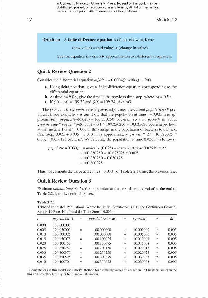
The growth is the growth_rate (r previously) times the current population (P pre-viously). For example, we can show that the population at time t = 0.025 h is ap-proximately population(0.025) = 100.250250 bacteria, so that growth is about growth_rate * population(0.025) = 0.1 * 100.250250 = 10.025025 bacteria per hour at that instant. For ∆t = 0.005 h, the change in the population of bacteria to the next time step, 0.025 + 0.005 = 0.030 h, is approximately growth * ∆t = 10.025025 * 0.005 = 0.050125 bacteria1. We calculate the population at time 0.030 h as follows:
population(0.030) = population(0.025) + (growth at time 0.025 h) * ∆t = 100.250250 + 10.025025 * 0.005 = 100.250250 + 0.050125 = 100.300375
Thus, we compute the value at the line t = 0.030 h of Table 2.2.1 using the previous line.
Quick Review Question 3Evaluate population(0.045), the population at the next time interval after the end of Table 2.2.1, to six decimal places.
1 Computations in this model use Euler's Method for estimating values of a function. In Chapter 6, we examine this and two other techniques for numeric integration.
Table 2.2.1 Table of Estimated Populations, Where the Initial Population is 100, the Continuous Growth Rate is 10% per Hour, and the Time Step is 0.005 h
t population(t) = population(t − ∆t) + (growth) * ∆t
0.000 100.0000000.005 100.050000 = 100.000000 + 10.000000 * 0.0050.010 100.100025 = 100.050000 + 10.005000 * 0.0050.015 100.150075 = 100.100025 + 10.010003 * 0.0050.020 100.200150 = 100.150075 + 10.015008 * 0.0050.025 100.250250 = 100.200150 + 10.020015 * 0.0050.030 100.300375 = 100.250250 + 10.025025 * 0.0050.035 100.350525 = 100.300375 + 10.030038 * 0.0050.040 100.400701 = 100.350525 + 10.035053 * 0.005
Definition A finite difference equation is of the following form:
(new value) = (old value) + (change in value)
Such an equation is a discrete approximation to a differential equation.
In order to view this proof accurately, the Overprint Preview Option must be checked in Acrobat Professional or Adobe Reader. Please contact your Customer Service Rep-
resentative if you have questions about finding the option.
Job Name: Cyan = PMS 300/356585t
© Copyright, Princeton University Press. No part of this book may be distributed, posted, or reproduced in any form by digital or mechanical means without prior written permission of the publisher.
System Dynamics Problems with Rate Proportional to Amount 23
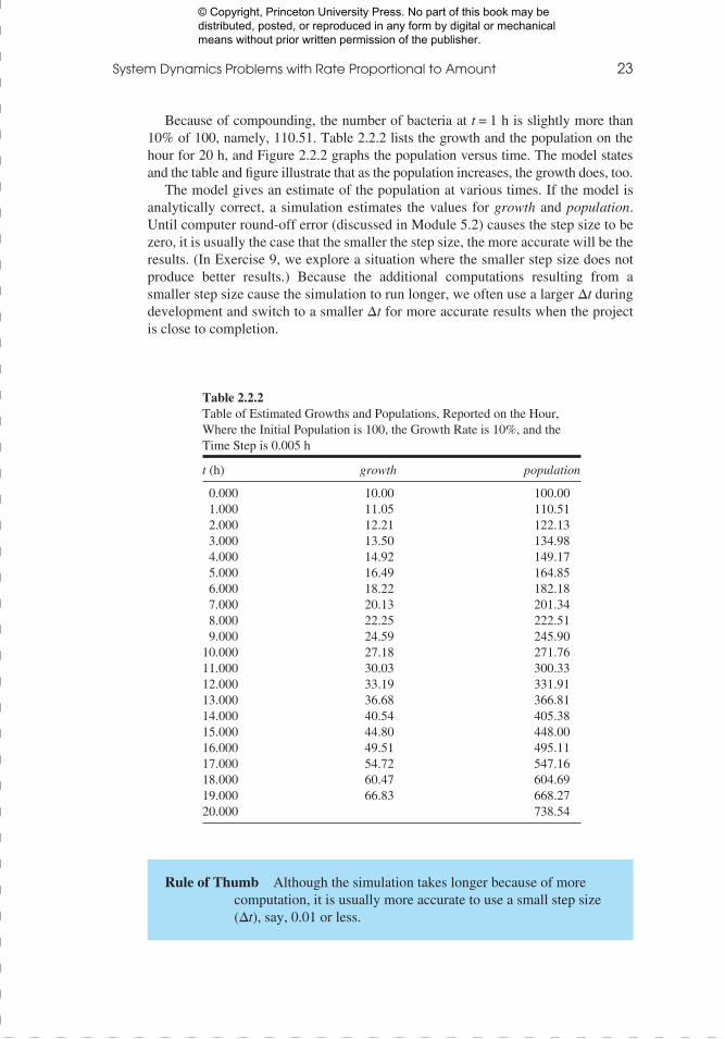
Table 2.2.2 Table of Estimated Growths and Populations, Reported on the Hour, Where the Initial Population is 100, the Growth Rate is 10%, and the Time Step is 0.005 h
t (h) growth population
0.000 10.00 100.00 1.000 11.05 110.51 2.000 12.21 122.13 3.000 13.50 134.98 4.000 14.92 149.17 5.000 16.49 164.85 6.000 18.22 182.18 7.000 20.13 201.34 8.000 22.25 222.51 9.000 24.59 245.9010.000 27.18 271.7611.000 30.03 300.3312.000 33.19 331.9113.000 36.68 366.8114.000 40.54 405.3815.000 44.80 448.0016.000 49.51 495.1117.000 54.72 547.1618.000 60.47 604.6919.000 66.83 668.2720.000 738.54
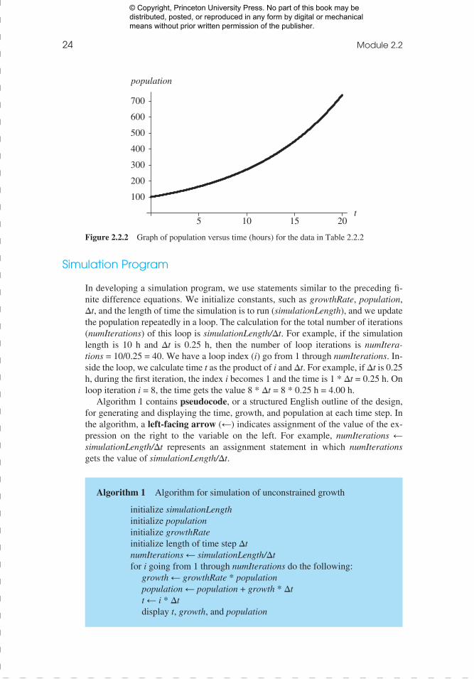
Because of compounding, the number of bacteria at t = 1 h is slightly more than 10% of 100, namely, 110.51. Table 2.2.2 lists the growth and the population on the hour for 20 h, and Figure 2.2.2 graphs the population versus time. The model states and the table and figure illustrate that as the population increases, the growth does, too.
The model gives an estimate of the population at various times. If the model is analytically correct, a simulation estimates the values for growth and population. Until computer round-off error (discussed in Module 5.2) causes the step size to be zero, it is usually the case that the smaller the step size, the more accurate will be the results. (In Exercise 9, we explore a situation where the smaller step size does not produce better results.) Because the additional computations resulting from a smaller step size cause the simulation to run longer, we often use a larger ∆t during development and switch to a smaller ∆t for more accurate results when the project is close to completion.
Rule of Thumb Although the simulation takes longer because of more computation, it is usually more accurate to use a small step size (∆t), say, 0.01 or less.
In order to view this proof accurately, the Overprint Preview Option must be checked in Acrobat Professional or Adobe Reader. Please contact your Customer Service Rep-
resentative if you have questions about finding the option.
Job Name: Cyan = PMS 300/356585t
© Copyright, Princeton University Press. No part of this book may be distributed, posted, or reproduced in any form by digital or mechanical means without prior written permission of the publisher.
24 Module 2.2
Simulation Program
In developing a simulation program, we use statements similar to the preceding fi-nite difference equations. We initialize constants, such as growthRate, population, ∆t, and the length of time the simulation is to run (simulationLength), and we update the population repeatedly in a loop. The calculation for the total number of iterations (numIterations) of this loop is simulationLength/∆t. For example, if the simulation length is 10 h and ∆t is 0.25 h, then the number of loop iterations is numItera-tions = 10/0.25 = 40. We have a loop index (i) go from 1 through numIterations. In-side the loop, we calculate time t as the product of i and ∆t. For example, if ∆t is 0.25 h, during the first iteration, the index i becomes 1 and the time is 1 * ∆t = 0.25 h. On loop iteration i = 8, the time gets the value 8 * ∆t = 8 * 0.25 h = 4.00 h.
Algorithm 1 contains pseudocode, or a structured English outline of the design, for generating and displaying the time, growth, and population at each time step. In the algorithm, a left-facing arrow (←) indicates assignment of the value of the ex-pression on the right to the variable on the left. For example, numIterations ← simulationLength/∆t represents an assignment statement in which numIterations gets the value of simulationLength/∆t.
Algorithm 1 Algorithm for simulation of unconstrained growth
initialize simulationLengthinitialize populationinitialize growthRateinitialize length of time step ∆t numIterations ← simulationLength/∆tfor i going from 1 through numIterations do the following:
growth ← growthRate * populationpopulation ← population + growth * ∆tt ← i * ∆tdisplay t, growth, and population
5 10 15 20t
100
200
300
400
500
600
700
population
Figure 2.2.2 Graph of population versus time (hours) for the data in Table 2.2.2
In order to view this proof accurately, the Overprint Preview Option must be checked in Acrobat Professional or Adobe Reader. Please contact your Customer Service Rep-
resentative if you have questions about finding the option.
Job Name: Cyan = PMS 300/356585t
© Copyright, Princeton University Press. No part of this book may be distributed, posted, or reproduced in any form by digital or mechanical means without prior written permission of the publisher.
System Dynamics Problems with Rate Proportional to Amount 25
If we do not need to display growth (derivative) at each step and the length of a step (∆t) is constant throughout the simulation, we can calculate the constant growth rate per step (growthRatePerStep) before the loop, as follows:
growthRatePerStep ← growthRate * ∆t
Within the loop, we do not compute growth but estimate population as follows:
population ← population + growthRatePerStep * population
Thus, within the loop, we have two assignments instead of three and two multiplica-tions instead of three, saving time in a lengthy simulation. The revised algorithm appears as Algorithm 2.
Analytical Solution: Introduction
We can solve the preceding model analytically for unconstrained growth, which is
the differential equation dPdt
P= 0 10. with initial condition P0 = 100, as follows:
P = 100 e0.10t
The next three sections develop the analytical solution. The first section starts the explanation using indefinite integrals, while the second section begins the discussion using derivatives without using integrals. Thus, you may select the section that matches your calculus background. The third section completes the development of the analytical solution for both tracks. Those without calculus background may go immediately to the section “Completion of the Analytical Solution.”
When it is possible to solve a problem analytically, we should usually do so. We have employed simulation of unconstrained growth with a system dynamic tool as an introduction to fundamental concepts and as a building block to more complex problems for which no analytical solutions exist.
Algorithm 2 Alternative algorithm to Algorithm 1 for simulation of uncon-strained growth that does not display growth
initialize simulationLengthinitialize populationinitialize growthRateinitialize ∆tgrowthRatePerStep ← growthRate * ∆tnumIterations ← simulationLength/∆tfor i going from 1 through numIterations do the following:
population ← population + growthRatePerStep * populationt ← i * ∆tdisplay t and population
In order to view this proof accurately, the Overprint Preview Option must be checked in Acrobat Professional or Adobe Reader. Please contact your Customer Service Rep-
resentative if you have questions about finding the option.
Job Name: Cyan = PMS 300/356585t
© Copyright, Princeton University Press. No part of this book may be distributed, posted, or reproduced in any form by digital or mechanical means without prior written permission of the publisher.
26 Module 2.2
Analytical Solution: Explanation with Indefinite Integrals (Optional)
We can solve the differential equation dPdt
P= 0 10. using a technique called separa-
tion of variables. First, we move all terms involving P to one side of the equation and all those involving t to the other. Leaving 0.10 on the right, we have the following:
1 0 10PdP dt= .
Then, we integrate both sides of the equation, as follows:
1 0 10PdP dt∫ = ∫ .
ln |P| = 0.10t + C for an arbitrary constant C
We solve for |P| by taking the exponential function of both sides and using the fact that the exponential and natural logarithmic functions are inverses of each other.
e eP e e A e
P t C
t C t
ln| | .
. .
== =
+0 10
0 10 0 10
where A = eC. Solving for P, we have
P = (±A)e0.10t
or
P = ke0.10t
where k = (±A) is a constant.
Analytical Solution: Explanation with Derivatives (Optional)
We can solve the differential equation dPdt
P= 0 10. for P analytically by finding a
function whose derivative is 0.10 times the function itself. The only functions that are their own derivative are exponential functions of the following form:
f(t) = ket, where k is a constant
For example, the derivative of 5et is 5et. To obtain a factor of 0.10 through use of the chain rule, we have the general solution
P = ke0.10t
In order to view this proof accurately, the Overprint Preview Option must be checked in Acrobat Professional or Adobe Reader. Please contact your Customer Service Rep-
resentative if you have questions about finding the option.
Job Name: Cyan = PMS 300/356585t
© Copyright, Princeton University Press. No part of this book may be distributed, posted, or reproduced in any form by digital or mechanical means without prior written permission of the publisher.
System Dynamics Problems with Rate Proportional to Amount 27
For example, if P = 5e0.10t, we have
dPdt
d edt
d edt
e et t
t t= = = =( ) ( ) ( . ) . ( ). .
. .5 5 5 0 10 0 10 50 10 0 10
0 10 0 10 == 0 10. P
Completion of the Analytical Solution
Thus, the general solution to dPdt
P= 0 10. is P = ke0.10t for a constant k. Using the
initial condition that P0 = 100, we can determine a particular value of k and, thus, a particular solution of the form P = ke0.10t. Substituting 0 for t and 100 for P, we have the following:
100 = ke0.10(0) = ke0 = k(1) = k
The constant is the initial population. For this example,
P = 100e0.10t
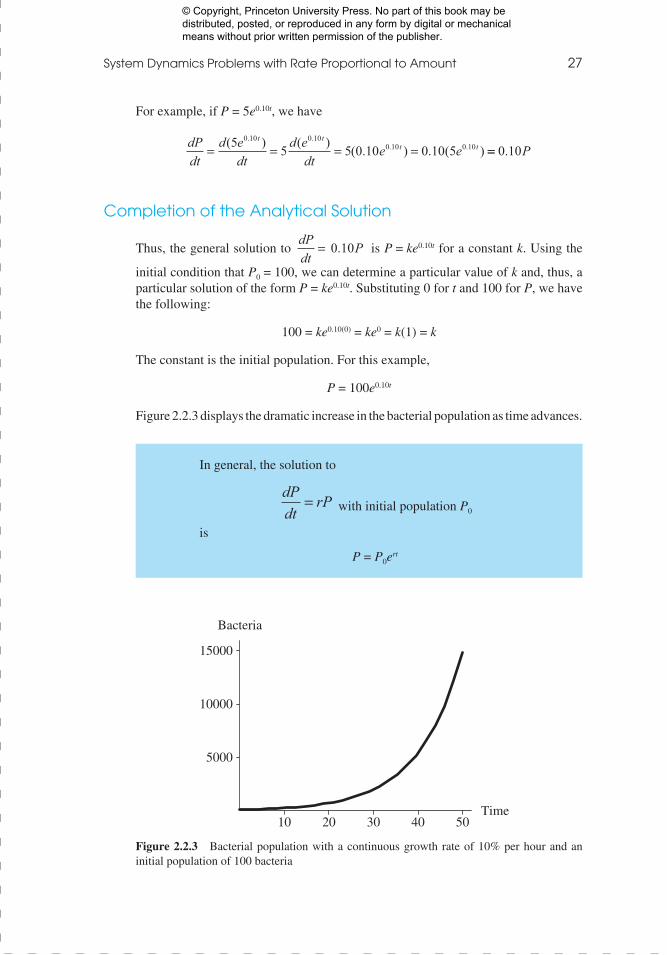
Figure 2.2.3 displays the dramatic increase in the bacterial population as time advances.
In general, the solution to
dPdt
rP= with initial population P0
is
P = P0ert
10 20 30 40 50Time
Bacteria
5000
10000
15000
Figure 2.2.3 Bacterial population with a continuous growth rate of 10% per hour and an initial population of 100 bacteria
In order to view this proof accurately, the Overprint Preview Option must be checked in Acrobat Professional or Adobe Reader. Please contact your Customer Service Rep-
resentative if you have questions about finding the option.
Job Name: Cyan = PMS 300/356585t
© Copyright, Princeton University Press. No part of this book may be distributed, posted, or reproduced in any form by digital or mechanical means without prior written permission of the publisher.
28 Module 2.2
Quick Review Question 4
Give the solution of the differential equation
dPdt
P= 0 03. , where P0 = 57
The simulated values for the bacterial population are slightly less than those the model P = 100e0.10t determines. For example, after 20 h, a simulation may display, to two decimal places, a population of 738.54. However, 100e0.10(20), expressed to two decimal places, is 738.91. The simulation compounds the population every step, and, in this case, the step size is ∆t = 0.005 h. The analytic model compounds the popula-tion continuously; that is, as the step size goes to zero and the number of steps goes to infinity approaches, the simulated values approach the analytic solution.
Both the analytic model and simulation produce valid estimates of the population of bacteria. After 20 h, the number of bacteria will be an integer, not a decimal num-ber, such as 738.54 or 738.91. Moreover, the population probably does not grow in an ideal fashion with a 10%-per-hour growth rate at every instant. Both the analytic model and the simulation produce estimates of the population at various times.
Further Refinement
We can refine the model further by having separate parameters for birth rate and death rate instead of the combined growth rate. Thus,
growth_rate = birth_rate – death_rate
Unconstrained Decay
The rate of change of the mass of a radioactive substance is proportional to the mass of the substance, and the constant of proportionality is negative. Thus, the mass de-cays with time. For example, the constant of proportionality for radioactive car-bon-14 is approximately –0.000120968. The continuous decay rate is about 0.0120968% per year, and the differential equation is as follows, where Q is the quantity (mass) of carbon-14:
dQdt
Q= −0.000120968
As indicated in the section “Completion of the Analytical Solution,” the analytical solution to this equation is
Q = Q0e-0.000120968t
After 10,000 yr, only about 29.8% of the original quantity of carbon-14 remains, as the following shows:
Q = Q0e-0.000120968(10,000) = 0.298292Q0
In order to view this proof accurately, the Overprint Preview Option must be checked in Acrobat Professional or Adobe Reader. Please contact your Customer Service Rep-
resentative if you have questions about finding the option.
Job Name: Cyan = PMS 300/356585t
© Copyright, Princeton University Press. No part of this book may be distributed, posted, or reproduced in any form by digital or mechanical means without prior written permission of the publisher.
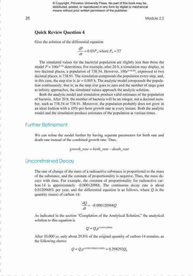
System Dynamics Problems with Rate Proportional to Amount 29
Figure 2.2.4 displays the decay of carbon-14 with time.Carbon dating uses the amount of carbon-14 in an object to estimate the age of
an object. All living organisms accumulate small quantities of carbon-14, but accu-mulation stops when the organism dies. For example, we can compare the proportion of carbon-14 in living bone to that in the bone of a mummy and estimate the age of the mummy using the model.
Example 1
Suppose the proportion of carbon-14 in a mummy is only about 20% of that in a liv-ing human. To estimate the age of the mummy, we use the preceding model with the information that Q = 0.20Q0. Substituting into the analytical model, we have
0.20Q0 = Q0e-0.000120968t
After canceling Q0, we solve for t by taking the natural logarithm of both sides of the equation. Because the natural logarithm and the exponential functions are inverses of each other, we have the following:
ln(0.20) = ln( e-0.000120968t) = –0.000120968t
t = ln(0.20)/(–0.000120968) ≈ 13,305 yr
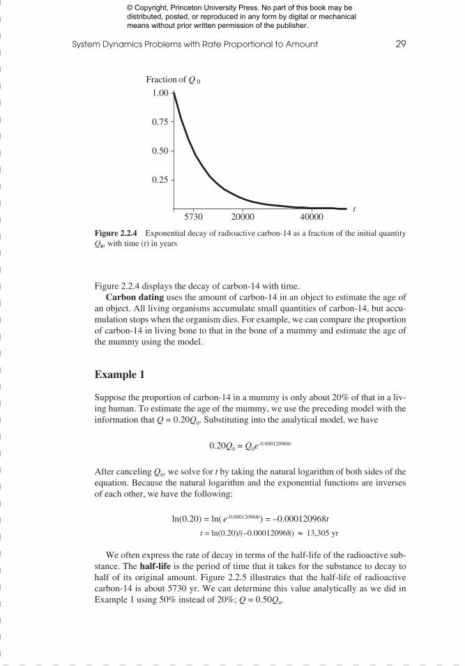
We often express the rate of decay in terms of the half-life of the radioactive sub-stance. The half-life is the period of time that it takes for the substance to decay to half of its original amount. Figure 2.2.5 illustrates that the half-life of radioactive carbon-14 is about 5730 yr. We can determine this value analytically as we did in Example 1 using 50% instead of 20%; Q = 0.50Q0.
5730 20000 40000t
Fraction of Q 0
0.25
0.50
0.75
1.00
Figure 2.2.4 Exponential decay of radioactive carbon-14 as a fraction of the initial quantity Q0, with time (t) in years
In order to view this proof accurately, the Overprint Preview Option must be checked in Acrobat Professional or Adobe Reader. Please contact your Customer Service Rep-
resentative if you have questions about finding the option.
Job Name: Cyan = PMS 300/356585t
© Copyright, Princeton University Press. No part of this book may be distributed, posted, or reproduced in any form by digital or mechanical means without prior written permission of the publisher.
30 Module 2.2
Quick Review Question 5
Radium-226 has a continuous decay rate of about 0.0427869% per year. Determine its half-life in whole years.
Reports for System Dynamics Models
The fifth step of the modeling process discussed in Module 1.2 is to “Report on the model.” The following summarizes the items that would be included in a report for a system dynamics model:
a. Analysis of the problem: We begin by describing the problem, such as to model the growth of bacteria in media.
b. Model design: In this section, we should list simplifying assumptions, such
as those in the section “Differential Equation”; equations, such as dPdt
P= 0 10.
with P0 = 100; reasoning for choices of constants, such as an instantaneous growth rate of 10%; the basic time step, such as hour; and other units. A dia-gram of the model, such as in Figure 2.2.1, is also appropriate to include.
c. Model solution: This part should contain the analytical solution or an algo-rithm, such as Algorithm 1.
d. Results and conclusions: Part d should include simulation tables, such as Table 2.2.2, and graphs, such as Figure 2.2.2. Moreover, the section should contain an explanation of verification accomplished by comparing the results to real data when available, descriptions of the outcomes of various scenar-
Definition The half-life is the period of time that it takes for a radioactive substance to decay to half of its original amount.
5730 20000 40000t
Fraction of Q 0
0.25
0.50
0.75
1.00
Figure 2.2.5 The half-life of radioactive carbon-14 indicated as 5730 yr
In order to view this proof accurately, the Overprint Preview Option must be checked in Acrobat Professional or Adobe Reader. Please contact your Customer Service Rep-
resentative if you have questions about finding the option.
Job Name: Cyan = PMS 300/356585t
© Copyright, Princeton University Press. No part of this book may be distributed, posted, or reproduced in any form by digital or mechanical means without prior written permission of the publisher.
System Dynamics Problems with Rate Proportional to Amount 31
ios, a discussion of our conclusions with support from the results, and sug-gestions for model refinement.
e. Appendices: Usually, a copy of the file created with a system dynamics tool should be submitted with this report. Besides the model, this file should con-tain appropriate documentation, such as a text box with the authors’ names, date, module and problem number, and problem description.
Exercises
Answers to marked exercises appear in the appendix “Answers to Selected Exercises.”
1. a. For an initial population of 100 bacteria and a continuous growth rate of 10% per hour, determine the number of bacteria at the end of one week.
b. How long will it take the population to double?2. a. Suppose the initial population of a certain animal is 15,000 and its con-
tinuous growth rate is 2% per year. Determine the population at the end of 20 yr.
b. Suppose we are performing a simulation of the population using a step size of 0.083 yr. Determine the growth and the population at the end of the first three time steps.
3. Adjust the model in Figure 2.2.1 to accommodate birth rate and death rate instead of just growth rate.
4. a. Newton’s Law of Heating and Cooling states that the rate of change of the temperature (T) with respect to time (t) of an object is proportional to the difference between the temperatures of the object and of its surround-ings. Suppose the temperature of the surroundings is 25 ̊ C. Write the dif-ferential equation that models Newton’s Law.
b. Solve this equation for T as a function of time t. c. Suppose cold water at 6 ̊ C is placed in a room that has temperature 25 ̊ C.
After 1 h, the temperature of the water is 20 ̊ C. Determine all constants in the equation for T.
d. What is the temperature of the water after 15 minutes (min)? e. How long will it take for the water to warm to room temperature?5. a. Suppose someone, whose temperature is originally 37 ̊ C, is murdered in a
room that has constant temperature 25 ̊ C. The temperature is measured as 28 ̊ C when the body is found and at 27 ̊ C 1 h later. How long ago was the murder committed from discovery of the body? See Exercise 4 for New-ton’s Law of Heating and Cooling.
b. Suppose we are performing a simulation using a step size of 0.004 h. Using the decay rate from Part a, determine the temperature at the end of the first three time steps after discovery of the body.
6. a. What proportion of the original quantity of carbon-14 is left after 30,000 yr?
b. If 60% is left, how old is the item?7. a. The half-life of radioactive strontium-90 is 29 yr. Give the model for the
quantity present as a function of time. b. What proportion of strontium-90 is present after 10 yr?
In order to view this proof accurately, the Overprint Preview Option must be checked in Acrobat Professional or Adobe Reader. Please contact your Customer Service Rep-
resentative if you have questions about finding the option.
Job Name: Cyan = PMS 300/356585t
© Copyright, Princeton University Press. No part of this book may be distributed, posted, or reproduced in any form by digital or mechanical means without prior written permission of the publisher.
32 Module 2.2
c. After 50 yr? d. How long will it take for the quantity to be 15% of the original amount?8. Suppose an investment has approximately a continuous growth rate of 9.3%.
Calculate analytically the value of an initial investment of $500 after a. 10 yr b. 20 yr c. 30 yr d. 40 yr d. How long will it take for the value to double? e. How long to quadruple?9. Suppose the amount of deposited ash, A, in millimeters (mm) is a function of
time t in days. Suppose the model states that the rate of change of ash with respect to time is 4 mm/day and the initial quantity is 3 mm.
a. Using a step size of 0.5 days (da), estimate the amount of ash when t = 1 da.
b. Repeat Part a using a step size of 0.25 da. c. Does the smaller step size change the result? d. Solve the model for A. e. What kind of function do you obtain?
Projects
For additional projects, see Module 7.1, “Radioactive Chains—Never the Same Again”; Module 7.2, “Turnover and Turmoil—Blood Cell Populations”; Module 7.3, “Deep Trouble—Ideal Gas Laws and Scuba Diving”; Module 7.4, “What Goes Around Comes Around—The Carbon Cycle”; after completion of “System Dynam-ics Tool: Tutorial 2,” Module 7.9, “Transmission of Nerve Impulses: Learning from the Action Potential Heroes”; Module 7.12 “Mercury Pollution—Getting on Our Nerves.”
1. Develop a model for Newton’s Law of Heating and Cooling (see Exercise 4). Using this model, answer the questions of Exercises 4 and 5.
2. In 1854, Dr. John Snow, the father of epidemiology, identified a particular London water pump as the point source of the Broad Street cholera epidemic, which spread in a radial fashion from the pump. Model such a spread of dis-ease assuming that the rate of change of the number of cases of cholera is proportional to the square root of the number of cases.
3. Develop a model for Exercise 8. 4. A young professional would like to save enough money to pay cash for a new
car. Develop a model to determine when such a purchase will be possible. Take into account the following issues: The price of a new car is rising due to inflation. The buyer plans to trade in a car, which is depreciating. This person already has some savings and plans to make regular monthly payments. Thus, use a ∆t value of 1 mo. Assume appropriate rates and values.
Develop a spreadsheet for each of Projects 5–8.
5. Exercise 26. Exercise 47. Exercise 58. Exercise 8
In order to view this proof accurately, the Overprint Preview Option must be checked in Acrobat Professional or Adobe Reader. Please contact your Customer Service Rep-
resentative if you have questions about finding the option.
Job Name: Cyan = PMS 300/356585t
© Copyright, Princeton University Press. No part of this book may be distributed, posted, or reproduced in any form by digital or mechanical means without prior written permission of the publisher.
System Dynamics Problems with Rate Proportional to Amount 33
Answers to Quick Review Questions
1. a. Average velocity from 1 to 2 s =
s s( ) ( ) . .3 13 1
11 9 21 12
−−
= −
= 0.3 m/s
b. Average velocity from 1 to 3 s =
s s( ) ( ) . .2 12 1
21 4 21 11
−−
= −
= –4.6 m/s
c. b = 3 s, s(b) = 11.9 m, ∆t = 2 s, b – ∆t = 1 s, s(b – ∆t) = 21.1 m, ∆s = 11.9 – 21.1 = –9.2 m
2. a. Q(t) = Q(t – ∆t) + ∆Q, where ∆Q = –0.0004Q(t – ∆t)∆t and Q(0) = 200 b. t – ∆t = 9.0 – 0.5 = 8.5 s c. ∆Q = 199.28 – 199.32 = –0.043. 100.450901 growth = 100.400701 * 0.10 = 10.040070 Thus, population(0.045) = 100.400701 + 10.040070 * 0.005 = 100.4509014. P = 57e0.03t
5. 1620. Reasoning:
Q = Q0 e -0.000427869t
For Q = 0.50Q0, 0.50Q0 = Q0 e -0.000427869t or 0.50 = e -0.000427869t
ln(0.50) = –0.000427869tt = ln(0.50)/(–0.000427869) = 1620
Reference
Zill, Dennis G. 2013. A First Course in Differential Equations with Modeling Ap-plications, 10th ed. Belmont, CA. Brooks-Cole Publishing (Cengage Learning).
In order to view this proof accurately, the Overprint Preview Option must be checked in Acrobat Professional or Adobe Reader. Please contact your Customer Service Rep-
resentative if you have questions about finding the option.
Job Name: Cyan = PMS 300/356585t
© Copyright, Princeton University Press. No part of this book may be distributed, posted, or reproduced in any form by digital or mechanical means without prior written permission of the publisher.
System Dynamics Problems with Rate Proportional to Amount 35
tential in their new environments because they are very adaptable to habitat and food sources, they have few or less-fit competitors, and few to no predators.
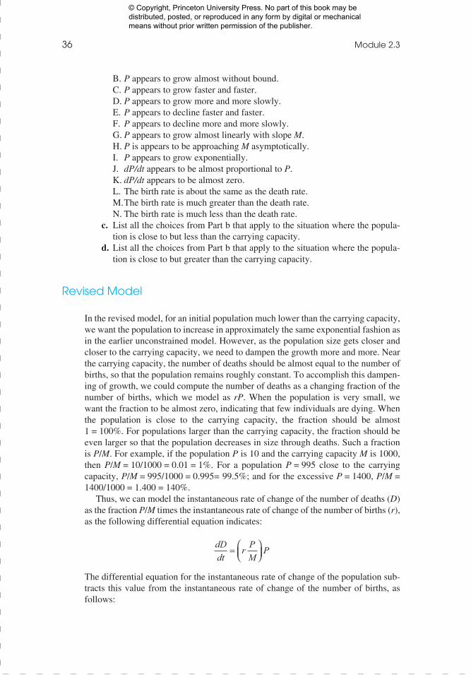
Carrying Capacity
In Module 2.2, “Unconstrained Growth and Decay,” we considered a population growing without constraints, such as competition for limited resources. For such a population, P, with instantaneous growth rate, r, the rate of change of the population has the following differential equation model:
dPdt
rP=
With initial population P0, we saw that the analytical solution is P = P0ert. In that
module, we also developed the following finite difference equation for the change in P from one time to the next, which we used in simulations:
∆P = P(t) – P(t – ∆t) = (r P(t – ∆t)) ∆t
Simulation and analytical solution graphs in Figures 2.2.2 and 2.2.3, respectively, of Module 2.2 display the exponential growth of unconstrained growth.
After developing such a model in Step 2 of the modeling process and solving the model (Step 3) as before, we should verify that the solution (Step 4) agrees with real data. However, as the introduction indicates, no confined population can grow with-out bound. Competition for food, shelter, and other resources eventually limits the possible growth. For example, suppose a deer refuge can support at most 1000 deer. We say that the carrying capacity (M) for the deer in the refuge is 1000.
Quick Review Question 1
Cycling back to Step 2 of the modeling process, this question begins refinement of the population model to accommodate descriptions of population growth from the “Introduction” of this module.
a. Determine any additional variable and its units. b. Consider the relationship between the number of individuals (P) and carry-
ing capacity (M) as time (t) increases. List all the statements below that apply to the situation where the population is much smaller than the carrying capacity.
A. P appears to grow almost proportionally to t.
Definition The carrying capacity for an organism in an area is the maxi-mum number of organisms that the area can support.
In order to view this proof accurately, the Overprint Preview Option must be checked in Acrobat Professional or Adobe Reader. Please contact your Customer Service Rep-
resentative if you have questions about finding the option.
Job Name: Cyan = PMS 300/356585t
© Copyright, Princeton University Press. No part of this book may be distributed, posted, or reproduced in any form by digital or mechanical means without prior written permission of the publisher.
36 Module 2.3
B. P appears to grow almost without bound. C. P appears to grow faster and faster. D. P appears to grow more and more slowly. E. P appears to decline faster and faster. F. P appears to decline more and more slowly. G. P appears to grow almost linearly with slope M. H. P is appears to be approaching M asymptotically. I. P appears to grow exponentially. J. dP/dt appears to be almost proportional to P. K. dP/dt appears to be almost zero. L. The birth rate is about the same as the death rate. M. The birth rate is much greater than the death rate. N. The birth rate is much less than the death rate.c. List all the choices from Part b that apply to the situation where the popula-
tion is close to but less than the carrying capacity.d. List all the choices from Part b that apply to the situation where the popula-
tion is close to but greater than the carrying capacity.
Revised Model
In the revised model, for an initial population much lower than the carrying capacity, we want the population to increase in approximately the same exponential fashion as in the earlier unconstrained model. However, as the population size gets closer and closer to the carrying capacity, we need to dampen the growth more and more. Near the carrying capacity, the number of deaths should be almost equal to the number of births, so that the population remains roughly constant. To accomplish this dampen-ing of growth, we could compute the number of deaths as a changing fraction of the number of births, which we model as rP. When the population is very small, we want the fraction to be almost zero, indicating that few individuals are dying. When the population is close to the carrying capacity, the fraction should be almost 1 = 100%. For populations larger than the carrying capacity, the fraction should be even larger so that the population decreases in size through deaths. Such a fraction is P/M. For example, if the population P is 10 and the carrying capacity M is 1000, then P/M = 10/1000 = 0.01 = 1%. For a population P = 995 close to the carrying capacity, P/M = 995/1000 = 0.995= 99.5%; and for the excessive P = 1400, P/M = 1400/1000 = 1.400 = 140%.
Thus, we can model the instantaneous rate of change of the number of deaths (D) as the fraction P/M times the instantaneous rate of change of the number of births (r), as the following differential equation indicates:
dDdt
r PM
P=
The differential equation for the instantaneous rate of change of the population sub-tracts this value from the instantaneous rate of change of the number of births, as follows:
In order to view this proof accurately, the Overprint Preview Option must be checked in Acrobat Professional or Adobe Reader. Please contact your Customer Service Rep-
resentative if you have questions about finding the option.
Job Name: Cyan = PMS 300/356585t
© Copyright, Princeton University Press. No part of this book may be distributed, posted, or reproduced in any form by digital or mechanical means without prior written permission of the publisher.
System Dynamics Problems with Rate Proportional to Amount 37
dPdt
rP r PM
P
births deaths
= −
( )��� � �� ��
or
dPdt
r PM
P= −
1 (1)
For the discrete simulation, where P(t – 1) is the population estimate at time t – 1, the number of deaths from time t – 1 to time t is
∆ ∆D rP tM
P t t=−( )
−( ) =1
1 1 for
In general, we approximate the number of deaths from time (t – ∆t) to time t by mul-tiplying the corresponding value by ∆t, as follows:
∆∆
∆ ∆D rP t tM
P t t t=−( )
−( )
where P(t – ∆t) is the population estimate at (t – ∆t). Thus, the change in population from time (t – ∆t) to time t is the difference of the number of births and the number of deaths over that period:
∆P = births – deaths
∆ ∆ ∆∆
∆ ∆P rP t t t rP t tM
P t t t= −( )( ) −−( )
−( )births
death
� ��� ���ss
� ����� �����
= ( ) −−( )
−( )r tP t tM
P t t∆∆
∆1
or
∆∆
∆ ∆P kP t tM
P t t k r t= −−( )
−( )1 , where = (2)
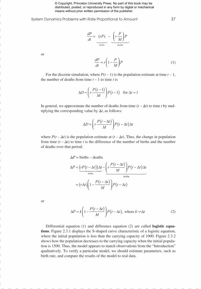
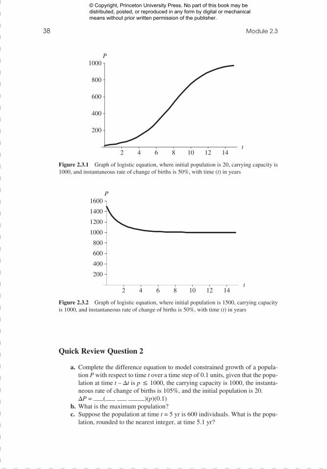
Differential equation (1) and difference equation (2) are called logistic equa-tions. Figure 2.3.1 displays the S-shaped curve characteristic of a logistic equation, where the initial population is less than the carrying capacity of 1000. Figure 2.3.2 shows how the population decreases to the carrying capacity when the initial popula-tion is 1500. Thus, the model appears to match observations from the “Introduction” qualitatively. To verify a particular model, we should estimate parameters, such as birth rate, and compare the results of the model to real data.
In order to view this proof accurately, the Overprint Preview Option must be checked in Acrobat Professional or Adobe Reader. Please contact your Customer Service Rep-
resentative if you have questions about finding the option.
Job Name: Cyan = PMS 300/356585t
© Copyright, Princeton University Press. No part of this book may be distributed, posted, or reproduced in any form by digital or mechanical means without prior written permission of the publisher.
38 Module 2.3
Quick Review Question 2
a. Complete the difference equation to model constrained growth of a popula-tion P with respect to time t over a time step of 0.1 units, given that the popu-lation at time t – ∆t is p ≤ 1000, the carrying capacity is 1000, the instanta-neous rate of change of births is 105%, and the initial population is 20.
∆P = ___(___ ___ _____)(p)(0.1)b. What is the maximum population?c. Suppose the population at time t = 5 yr is 600 individuals. What is the popu-
lation, rounded to the nearest integer, at time 5.1 yr?
2 4 6 8 10 12 14t
200
400
600
800
1000P
Figure 2.3.1 Graph of logistic equation, where initial population is 20, carrying capacity is 1000, and instantaneous rate of change of births is 50%, with time (t) in years
2 4 6 8 10 12 14t
200
400
600
800
1000
1200
1400
1600P
Figure 2.3.2 Graph of logistic equation, where initial population is 1500, carrying capacity is 1000, and instantaneous rate of change of births is 50%, with time (t) in years
In order to view this proof accurately, the Overprint Preview Option must be checked in Acrobat Professional or Adobe Reader. Please contact your Customer Service Rep-
resentative if you have questions about finding the option.
Job Name: Cyan = PMS 300/356585t
© Copyright, Princeton University Press. No part of this book may be distributed, posted, or reproduced in any form by digital or mechanical means without prior written permission of the publisher.
System Dynamics Problems with Rate Proportional to Amount 39
Equilibrium and Stability
The logistic equation with carrying capacity M = 1000 has an interesting property. If the initial population is less than 1000, as in Figure 2.3.1, the population increases to a limit of 1000. If the initial population is greater than 1000, as in Figure 2.3.2, the population decreases to the limit of 1000. Moreover, if the initial population is 1000, we see from Equation (1) that P/M = 1000/1000 = 1 and dP/dt = r(1 – 1)P = 0. In discrete terms, ∆P = 0. A population starting at the carrying capacity remains there. We say that M = 1000 is an equilibrium size for the population because the popula-tion remains steady at that value or P(t) = P(t – ∆t) = 1000 for all t > 0.
Quick Review Question 3
Give another equilibrium size for the logistic differential equation (1) or logistic dif-ference equation (2).
Even if an initial positive population does not equal the carrying capacity M = 1000, eventually, the population size tends to that value. We say that the solution P = 1000 to the logistic equation (1) or (2) is stable. By contrast, for a positive carry-ing capacity, the solution P = 0 is unstable. If the initial population is close to but not equal to zero, the population does not tend to that solution over time. For the logistic equation, any displacement of the initial population from the carrying capacity exhib-its the limiting behavior of Figure 2.3.1 or 2.3.2. In general, we say that a solution is stable if for a small displacement from the solution, P tends to the solution.
Exercises
1. Using calculus, solve the following: a. The differential equation (1), dP
dtr P
MP= −
1
Definitions An equilibrium solution for a differential equation is a solution where the derivative is always zero. An equilibrium solution for a difference equation is a solution where the change is always zero.
Definition Suppose that q is an equilibrium solution for a differential equa-tion dP/dt or a difference equation ∆P. The solution q is stable if there is an interval (a, b) containing q, such that if the initial pop-ulation P(0) is in that interval, then
1. P(t) is finite for all t > 0;2. As time, t, becomes larger and larger, P(t) approaches q.
The solution q is unstable if no such interval exists.
In order to view this proof accurately, the Overprint Preview Option must be checked in Acrobat Professional or Adobe Reader. Please contact your Customer Service Rep-
resentative if you have questions about finding the option.
Job Name: Cyan = PMS 300/356585t
© Copyright, Princeton University Press. No part of this book may be distributed, posted, or reproduced in any form by digital or mechanical means without prior written permission of the publisher.
40 Module 2.3
where the carrying capacity, M, is 1000, P0 = 20, and the instantaneous rate of change of the number of births, r, is 50%
b. The differential equation (1) in general2. Consider dy/dt = cos(t). a. Give all the equilibrium solutions. b. Using calculus, find a function y(t) that is a solution. c. Give the most general function y that is a solution.3. It has been reported that a mallard must eat 3.2 ounces (oz) of rice each day
to remain healthy. On the average, an acre of rice in a certain area yields 110 bushels (bu) per year; and a bushel of rice weighs 45 lb. Assuming that in the area 100 acres (ac) of rice are available for mallard consumption and mal-lards eat only rice, determine the carrying capacity for mallards in the area (Reinecke).
4. The Gompertz differential equation, which follows, is one of the best mod-els for predicting the growth of cancer tumors:
dNdt
kN MN
N N=
=ln , ( )0 0
where N is the number of cancer cells and k and M are constants. a. As N approaches M, what does dN/dt approach? b. Make the substitution u = ln(M/N) in the Gompertz equation to eliminate
N and convert the equation to be in terms of u. c. Using calculus, solve the transformed differential equation for u. d. Using the relationship between u and N from Part b, convert your answer
from Part c to be in terms of N. The result is the solution to the Gompertz differential equation.
e. Using calculus, verify that N(t) = MeNM
e ktln 0
−
is the solution to the Gom p -ertz differential equation.
f. Using the solution in Part e, what does N approach as t goes to infinity?5. a. Graph y = e-t. Match each of the following scenarios to a differential equation that might
model it. A. dP/dt = 0.05P B. dP/dt = 0.05P + e-t
C. dP/dt = 0.05(1 – e-t)P D. dP/dt = 0.05P – 0.0003P2 – 400 E. dP/dt = 0.05e-tP F. dP/dt = 0.05P – 0.0003P2
b. At first, a bacteria colony appears to grow without bound; but because of limited nutrients and space, the population eventually approaches a limit.
c. Because of degradation of nutrients, the growth of a bacterial colony be-comes dampened.
d. A bacterial colony has unlimited nutrients and space and grows without bound.
e. Because of adjustment to its new setting, a bacterial colony grows slowly at first before appearing to grow without bound.
f. Each day, a scientist removes a constant amount from the colony.6. Write an algorithm for simulation of constrained growth similar to Algo-
rithm 1 for simulation of unconstrained growth in Module 2.2.
In order to view this proof accurately, the Overprint Preview Option must be checked in Acrobat Professional or Adobe Reader. Please contact your Customer Service Rep-
resentative if you have questions about finding the option.
Job Name: Cyan = PMS 300/356585t
© Copyright, Princeton University Press. No part of this book may be distributed, posted, or reproduced in any form by digital or mechanical means without prior written permission of the publisher.
System Dynamics Problems with Rate Proportional to Amount 41
Projects
For additional projects, see Module 7.4, “What Goes Around Comes Around—The Carbon Cycle”; Module 7.5, “A Heated Debate—Global Warming”; and Module 7.6, “Plotting the Future: How Will the Garden Grow.”
1. Develop a model for constrained growth.2. Develop a model for the mallard population in Exercise 3. Have a converter
or variable for the number of acres of rice available for mallard consumption, and from this value, have the model compute the carrying capacity. Report on the effect of decreasing the number of acres of rice available (Reinecke).
3. In some situations, the carrying capacity itself is dynamic. For example, the performance of airplanes had one carrying capacity with piston engines and a higher limit with the advent of jet engines. Many think that human popula-tion growth over a limited period of time follows such a pattern as techno-logical changes enable more people to live on the available resources. In such cases, we might be able to model the carrying capacity itself as a logis-tic. Suppose M1 is the first carrying capacity, and M1 + M2 is the second. The differential equation for the carrying capacity M(t) as a function of time t would be as follows:
dM tdt
a M t M M t MM
( ) ( ( ) ) ( )= − −
−
1
1
2
1 for some constant a > 0
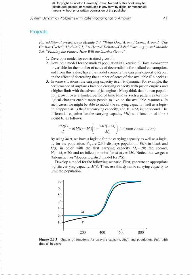
By using M(t), we have a logistic for the carrying capacity as well as a logis-tic for the population. Figure 2.3.3 displays population, P(t), in black and M(t) in color with the first carrying capacity M1 = 20; the second, M1 + M2 = 70; and an inflection point for M at t = 450. Notice that we get a “bilogistic,” or “doubly logistic,” model for P(t).
Develop a model for the following scenario. First, generate an appropriate logistic carrying capacity, M(t). Then, use this dynamic carrying capacity to limit the population.
200 400 600 800t
10
20
30
40
50
60
70
M
P
Figure 2.3.3 Graphs of functions for carrying capacity, M(t), and population, P(t), with time (t) in years
In order to view this proof accurately, the Overprint Preview Option must be checked in Acrobat Professional or Adobe Reader. Please contact your Customer Service Rep-
resentative if you have questions about finding the option.
Job Name: Cyan = PMS 300/356585t
© Copyright, Princeton University Press. No part of this book may be distributed, posted, or reproduced in any form by digital or mechanical means without prior written permission of the publisher.
42 Module 2.3
In a population study of England from 1541 to 1975, starting with a popu-lation of about 1 million, early islanders appear to have a carrying capacity of around 5 million people. However, beginning about 1800 with the advent of the Industrial Revolution, the carrying capacity appears to have increased to about 50 million people. The change in the concavity from concave up to concave down for this new logistic appears to occur in about 1850 (Meyer and Ausubel 1999).
4. Refer to Project 3 for a description of a logistic carrying-capacity function. Using that information, develop a model for the Japanese population from the year 1100 to 2000. With an initial population of 5 million, the island population was mainly a feudal society that leveled off to about 35 million. The industrial revolution came to Japan in the latter part of the nineteenth century, and the population rose rapidly over a 77-yr period, with the inflec-tion point occurring about 1908 (Meyer and Ausubel 1999).
5. Develop a model for the number of trout in a lake initially stocked with 400 trout. These fish increase at a rate of 15%, and the lake has a carrying capac-ity of 5000 trout. However, vacationers catch trout at a rate of 8%.
6. It has been estimated that for the Antarctic fin whale, r = 0.08, M = 400,000, and P0 = 70,000 in 1976. Model this population. Then, revise the model to consider harvesting the whales as a percentage of rM. Give various values for this percentage that lead to extinction and other values that lead to in-creases in the population. Estimate the maximum sustainable yield, or the percentage of rM that gives a constant population in the long term (Zill 2013).
7. Army ants on a 17-km2 island forage at a rate of 1500 m2/day, clearing the area almost completely of other insects. Once the ants have departed, it takes about 150 days for the number of other insects to recover in the area. Assume an initial number of 1million army ants and a growth rate of 3.6%, where the unit of time is a week. Model the population.
Answers to Quick Review Questions
1. a. carrying capacity, say M, in units of the population, such as deer or bacteria
b. B. P appears to grow almost without bound. C. P appears to grow faster and faster. I. P appears to grow exponentially. J. dP/dt appears to be almost proportional to P. M. The birth rate is much greater than the death rate. c. D. P appears to grow more and more slowly. H. P is appears to be approaching M asymptotically. K. dP/dt appears to be almost zero. L. The birth rate is about the same as the death rate. d. F. P appears to decline more and more slowly. H. P is appears to be approaching M asymptotically. K. dP/dt appears to be almost zero.
In order to view this proof accurately, the Overprint Preview Option must be checked in Acrobat Professional or Adobe Reader. Please contact your Customer Service Rep-
resentative if you have questions about finding the option.
Job Name: Cyan = PMS 300/356585t
© Copyright, Princeton University Press. No part of this book may be distributed, posted, or reproduced in any form by digital or mechanical means without prior written permission of the publisher.
System Dynamics Problems with Rate Proportional to Amount 43
L. The birth rate is about the same as the death rate.2. a. ∆P = 1.05(1 – p/1000)(p)(0.1) b. 1000 individuals c. 625 individuals because P + ∆P = 600 + 1.05(1 – 600/1000) 600(0.1) =
625.2 individuals 3. 0 because dP/dt = r(1 – P/M)P = r(1 – 0)0 = 0
References
Adams, C. E., and P. S. Maitland. 1998. “The Ruffe Population in Loch Lomond, Scotland: Its Introduction, Population Expansion, and Interaction with Native Species.” Journal of Great Lakes Research, 24: 249–262.
Fuller, P. G., J. Jacobs, J. Larson, and A. Fusaro. 2012. “Gymnocephalus cernuus.” USGS Nonindigenous Aquatic Species Database. Gainesville, FL. http://nas.er .usgs.gov/queries/FactSheet.aspx?speciesID=7 (accessed November 11, 2012)
Hajjar, R. 2002. “Introduced Species Summary Project: Ruffe (Gymnocephalus cer-nuus).” Columbia University. http://www.columbia.edu/itc/cerc/danoffburg/inva sion_bio/inv_spp_summ/Gymnocephalus cernuus.html (accessed November 11, 2012)
McLean, M. 1993. “Ruffe (Gymnocephalus cernuus) Fact Sheet.” Minnesota Sea Grant Program, Great Lakes Sea Grant Network, Duluth, MN. http://www.dnr .state.mn.us/invasives/aquaticanimals/ruffe/index.html (accessed January 7, 2013)
Meyer, Perrin S., and Jesse H. Ausubel. 1999. “Carrying Capacity: A Model with Logistically Varying Limits.” Technological Forecasting and Social Change, 61(3): 209–214.
Reinecke, Kenneth J. Personal communication. USGS, Pantuxent Wildlife Research Center. Beltsville Laboratory, 308-10300 Baltimore Avenue, Beltsville, MD 20705.
Sea Grant Pennsylvania. “Eurasian Ruffe: Gymnocephalus cernuus.” http://www .paseagrant.org/wp-content/uploads/2012/09/Ruffe2012.pdf (accessed January 7, 2013)
Zill, Dennis G. 2013. A First Course in Differential Equations with Modeling Ap-plications, 10th ed. Belmont, CA. Brooks-Cole Publishing (Cengage Learning).
In order to view this proof accurately, the Overprint Preview Option must be checked in Acrobat Professional or Adobe Reader. Please contact your Customer Service Rep-
resentative if you have questions about finding the option.
Job Name: Cyan = PMS 300/356585t
© Copyright, Princeton University Press. No part of this book may be distributed, posted, or reproduced in any form by digital or mechanical means without prior written permission of the publisher.
MODULE 2.4
System Dynamics Tool: Tutorial 2
Prerequisite: Module 2.1,“System Dynamics Tool: Tutorial 1”
Download
From the textbook’s website, download Tutorial 2 in PDF format and the uncon-strained file for your system dynamics tool. We recommend that you work through the tutorial and answer all Quick Review Questions using the corresponding software.
Introduction
This tutorial introduces the following functions and concepts, which subsequent modules employ for model formulation and solution using your system dynamics tool:
• Built-in functions and constants, such as the if-then-else construct, absolute value, initial value, exponential function, sine, pulse function, time, time step, and π
• Relational and logical operators• Comparative graphs• Graphical input• Conveyors, an optional topic useful for some of the later projects
In order to view this proof accurately, the Overprint Preview Option must be checked in Acrobat Professional or Adobe Reader. Please contact your Customer Service Rep-
resentative if you have questions about finding the option.
Job Name: Cyan = PMS 300/356585t
© Copyright, Princeton University Press. No part of this book may be distributed, posted, or reproduced in any form by digital or mechanical means without prior written permission of the publisher.
MODULE 2.5
Drug Dosage
Downloads
The text’s website has OneCompartAspirin and OneCompartDilantin files, which contain models for examples in this module, available for download in various sys-tem dynamics systems.
Introduction
Errors in the dispensing and administration of medications occur frequently. Although most do not result in great harm, some do. For instance, a Florida pharmacy dispensed 10 times the prescribed dose of a blood thinner to a mother of four, which resulted in her suffering a cerebral hemorrhage (Patel and Ross 2010). In other tragedies, a 10-mo-old infant died after receiving a 10-fold overdose of the chemotherapy agent Cisplatin (Fitzgerald and Wilson 1998), and three nurses were prosecuted for adminis-tering a 10-fold (fatal) overdose of penicillin to an infant (Ellis and Hartley 2004).
The National Quality Forum, a nonprofit whose mission involves enabling “pri-vate- and public-sector stakeholders to work together to craft and implement cross-cutting solutions to drive continuous quality improvement in the American health-care system,” has estimated that medication errors account for a conservative estimate of $21 billion in costs. This financial expenditure corresponds to serious preventable medication errors for 3.8 million hospital inpatients and 3.3 million out-patients per year (NQF 2010). These cases comprise an extraordinary amount of human suffering and, in some cases, death.
How do these errors occur? According to the Institute of Medicine, medication errors can be classified as errors in
ordering—incorrect drug or dosage;transcribing—incorrect frequency of administration or missed dosages;dispensing—incorrect drug, dosage, or timing;
In order to view this proof accurately, the Overprint Preview Option must be checked in Acrobat Professional or Adobe Reader. Please contact your Customer Service Rep-
resentative if you have questions about finding the option.
Job Name: Cyan = PMS 300/356585t
© Copyright, Princeton University Press. No part of this book may be distributed, posted, or reproduced in any form by digital or mechanical means without prior written permission of the publisher.
46 Module 2.5
administering—wrong dosage, technique;monitoring—not observing effects of medication.
Whether these errors result from poor communication of orders, poor product label-ing, or some other cause, the patients and their families suffer the consequences (IOM 2007).
It is not only health-care professionals who make mistakes in drug administra-tion. On June 28, 2003, an Oklahoma teenager died from an overdose of Tylenol (acetaminophen). Suffering from a migraine headache, she took twenty 500-mg cap-sules, two and one-half times the maximum dosage recommended in 24 h. Appar-ently, the quantity was enough of the drug to cause liver and kidney failure. Assum-ing that an over-the-counter analgesic was safe, she apparently did not read the label and made a fatal dosage error (Robert 2004).
There are prescribed dosages for various drugs, but how do we determine what the correct/effective dosage is? There are quite a number of factors that are consid-ered, including drug absorption, distribution, metabolism, and elimination. These factors are components of the quantitative science of pharmacokinetics.
One-Compartment Model of Single Dose
Metabolism of a drug in the human body is a complex system to represent in a model. Thus, in Step 2 of the modeling process, particularly for our first attempt, we should make simplifying assumptions about the drug and the body. A one-compart-ment model is a simplified representation of how a body processes a drug. In this model, we consider the body to be one homogeneous compartment, where distribu-tion is instantaneous, the concentration of the drug in the system (amount of drug/volume of blood) is proportional to the drug dosage, and the rate of elimination is proportional to the amount of drug in the system. The concentration of a drug instead of the absolute quantity is important because a quantity that might be appropriate for a small child could be ineffective for a large adult. A drug has a minimum effective concentration (MEC), which is the least amount of drug that is helpful, and a maxi-mum therapeutic concentration, or minimum toxic concentration (MTC), which is the largest amount that is helpful without having dangerous or intolerable side ef-fects. The therapeutic range for a drug consists of concentrations between the MEC and MTC. A drug’s half-life, or the amount of time for half the drug to be eliminated from the system, is useful for modeling as well as patient treatment. Often concen-trations and half-life are expressed in relationship to the drug in the plasma or blood serum. The total amount of blood in an adult’s body is approximately 5 liters (L), while the amount of plasma, or fluid that contains the blood cells, is about 3 L. Blood serum is the clear fluid that separates from blood when it clots, and an adult human has about 3 L of blood serum.
We begin by modeling the concentration in the body of aspirin (acetylsalicylic acid). For adults and children over the age of 12, the dosage for a headache is one or two 325-mg tablets every 4 h as necessary, up to 12 tablets/da. Analgesic effective-ness occurs at plasma levels of about 150 to 300 micrograms/milliliter (µg/mL), while toxicity may occur at plasma concentrations of 350 µg/mL. The plasma half-life of a dose from 300 to 650 mg is 3.1 to 3.2 h, with a larger dose having a longer half-life.
In order to view this proof accurately, the Overprint Preview Option must be checked in Acrobat Professional or Adobe Reader. Please contact your Customer Service Rep-
resentative if you have questions about finding the option.
Job Name: Cyan = PMS 300/356585t
© Copyright, Princeton University Press. No part of this book may be distributed, posted, or reproduced in any form by digital or mechanical means without prior written permission of the publisher.
System Dynamics Problems with Rate Proportional to Amount 47
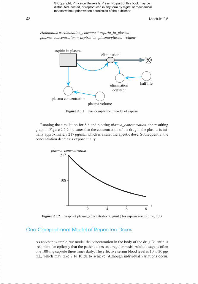
For simplicity, we assume a one-compartment model with the aspirin immedi-ately available in the plasma. A stock (box variable), aspirin_in_plasma, represents the mass of aspirin in the compartment, which is the person’s system, and has an ini-tial value of the mass of two aspirin, (2)(325 mg)(1000 µg/mg), where 1 milligram (mg) is equivalent to 1000 µg.
The flow from aspirin_in_plasma (elimination) is proportional to the amount pre-sent in the system, aspirin_in_plasma. Thus, the rate of change of the drug leaving the system is proportional to the quantity of drug in the system (aspirin_in_plasma, or Q in the following equation):
dQ/dt = –KQ
As Module 2.2, “Unconstrained Growth and Decay,” shows, the solution to this dif-ferential equation is as follows:
Q = Q0e-Kt
Using this solution, as Exercise 1 shows, the constant of proportionality K given earlier and elimination_constant in the system dynamics software model have the following relationship to the drug’s half-life (t1/2):
K = –ln(0.5)/t1/2
Pharmaceutical sources widely report a drug’s half-life.
Quick Review Question 1
Determine the elimination constant with units for aspirin, assuming a half-life of 3.2 h.
To compute aspirin’s plasma concentration (plasma_concentration) in a con-verter (variable), we have another converter for the volume of the system (plasma_volume) with a value of 3000 mL and appropriate connectors and equation. Figure 2.5.1 contains a one-compartment model for one dose of a drug, where the initial value of plasma_concentration is the dosage; and Equation Set 2.5.1 gives the cor-responding equations and values explicitly entered for the model of aspirin.
Quick Review Question 2
In terms of the variables in the model of Figure 2.5.1, give the equation for plasma_ concentration.
Equation Set 2.5.1
Explicitly entered equations and values for one-compartment model of aspirin:
half_life = 3.2 hplasma_volume = 3000 mLaspirin_in_plasma(0) = 2 * 325 * 1000 µgelimination_constant = –ln(0.5)/half_life
In order to view this proof accurately, the Overprint Preview Option must be checked in Acrobat Professional or Adobe Reader. Please contact your Customer Service Rep-
resentative if you have questions about finding the option.
Job Name: Cyan = PMS 300/356585t
© Copyright, Princeton University Press. No part of this book may be distributed, posted, or reproduced in any form by digital or mechanical means without prior written permission of the publisher.
48 Module 2.5
elimination = elimination_constant * aspirin_in_plasmaplasma_concentration = aspirin_in_plasma/plasma_volume
Running the simulation for 8 h and plotting plasma_concentration, the resulting graph in Figure 2.5.2 indicates that the concentration of the drug in the plasma is ini-tially approximately 217 µg/mL, which is a safe, therapeutic dose. Subsequently, the concentration decreases exponentially.
One-Compartment Model of Repeated Doses
As another example, we model the concentration in the body of the drug Dilantin, a treatment for epilepsy that the patient takes on a regular basis. Adult dosage is often one 100-mg capsule three times daily. The effective serum blood level is 10 to 20 µg/mL, which may take 7 to 10 da to achieve. Although individual variations occur,
eliminationaspirin in plasma
plasma volumeplasma concentration
eliminationconstant
half life
Figure 2.5.1 One-compartment model of aspirin
2 4 6 8t
108
217plasma concentration
Figure 2.5.2 Graph of plasma_concentration (µg/mL) for aspirin versus time, t (h)
In order to view this proof accurately, the Overprint Preview Option must be checked in Acrobat Professional or Adobe Reader. Please contact your Customer Service Rep-
resentative if you have questions about finding the option.
Job Name: Cyan = PMS 300/356585t
© Copyright, Princeton University Press. No part of this book may be distributed, posted, or reproduced in any form by digital or mechanical means without prior written permission of the publisher.
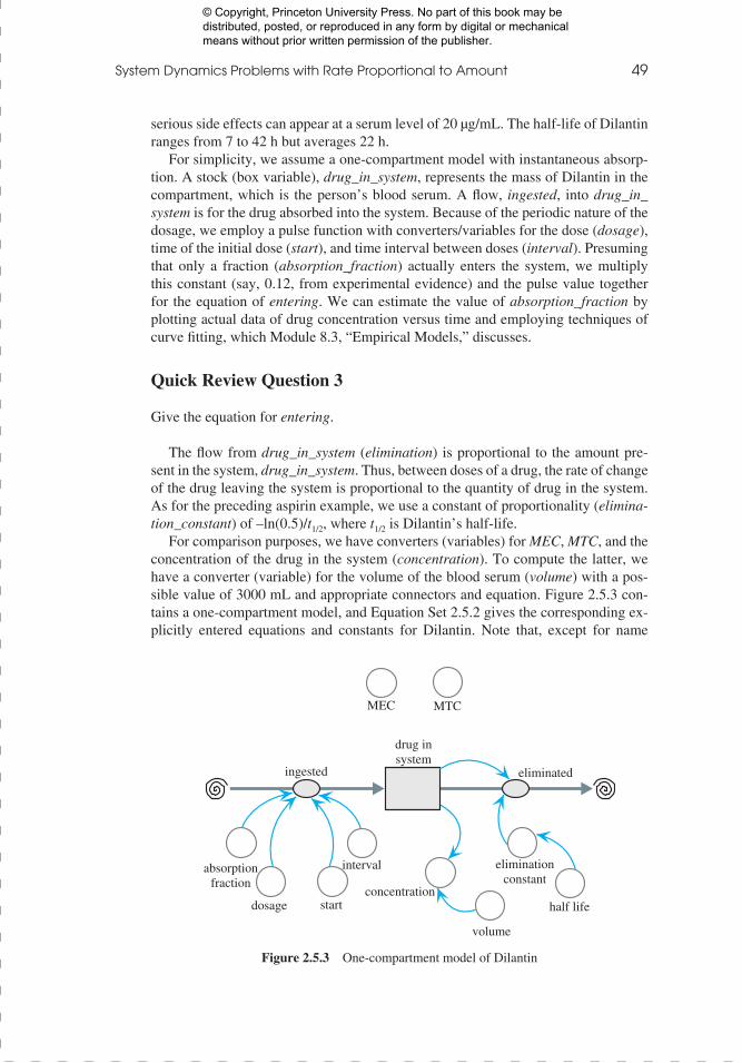
System Dynamics Problems with Rate Proportional to Amount 49
serious side effects can appear at a serum level of 20 µg/mL. The half-life of Dilantin ranges from 7 to 42 h but averages 22 h.
For simplicity, we assume a one-compartment model with instantaneous absorp-tion. A stock (box variable), drug_in_system, represents the mass of Dilantin in the compartment, which is the person’s blood serum. A flow, ingested, into drug_in_system is for the drug absorbed into the system. Because of the periodic nature of the dosage, we employ a pulse function with converters/variables for the dose (dosage), time of the initial dose (start), and time interval between doses (interval). Presuming that only a fraction (absorption_fraction) actually enters the system, we multiply this constant (say, 0.12, from experimental evidence) and the pulse value together for the equation of entering. We can estimate the value of absorption_fraction by plotting actual data of drug concentration versus time and employing techniques of curve fitting, which Module 8.3, “Empirical Models,” discusses.
Quick Review Question 3
Give the equation for entering.
The flow from drug_in_system (elimination) is proportional to the amount pre-sent in the system, drug_in_system. Thus, between doses of a drug, the rate of change of the drug leaving the system is proportional to the quantity of drug in the system. As for the preceding aspirin example, we use a constant of proportionality (elimina-tion_constant) of –ln(0.5)/t1/2, where t1/2 is Dilantin’s half-life.
For comparison purposes, we have converters (variables) for MEC, MTC, and the concentration of the drug in the system (concentration). To compute the latter, we have a converter (variable) for the volume of the blood serum (volume) with a pos-sible value of 3000 mL and appropriate connectors and equation. Figure 2.5.3 con-tains a one-compartment model, and Equation Set 2.5.2 gives the corresponding ex-plicitly entered equations and constants for Dilantin. Note that, except for name
Figure 2.5.3 One-compartment model of Dilantin
MEC MTC
dosage start
intervalabsorptionfraction
drug insystem
concentration
volume
eliminationconstant
half life
ingested eliminated
In order to view this proof accurately, the Overprint Preview Option must be checked in Acrobat Professional or Adobe Reader. Please contact your Customer Service Rep-
resentative if you have questions about finding the option.
Job Name: Cyan = PMS 300/356585t
© Copyright, Princeton University Press. No part of this book may be distributed, posted, or reproduced in any form by digital or mechanical means without prior written permission of the publisher.
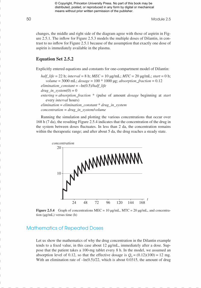
50 Module 2.5
changes, the middle and right side of the diagram agree with those of aspirin in Fig-ure 2.5.1. The inflow for Figure 2.5.3 models the multiple doses of Dilantin, in con-trast to no inflow for Figure 2.5.1 because of the assumption that exactly one dose of aspirin is immediately available in the plasma.
Equation Set 2.5.2
Explicitly entered equations and constants for one-compartment model of Dilantin:
half_life = 22 h; interval = 8 h; MEC = 10 µg/mL; MTC = 20 µg/mL; start = 0 h; volume = 3000 mL; dosage = 100 * 1000 µg; absorption_fraction = 0.12
elimination_constant = –ln(0.5)/half_lifedrug_in_system(0) = 0entering = absorption_fraction * (pulse of amount dosage beginning at start
every interval hours) elimination = elimination_constant * drug_in_systemconcentration = drug_in_system/volume
Running the simulation and plotting the various concentrations that occur over 168 h (7 da), the resulting Figure 2.5.4 indicates that the concentration of the drug in the system between doses fluctuates. In less than 2 da, the concentration remains within the therapeutic range; and after about 5 da, the drug reaches a steady state.
Mathematics of Repeated Doses
Let us show the mathematics of why the drug concentration in the Dilantin example tends to a fixed value, in this case about 12 µg/mL, immediately after a dose. Sup-pose that the patient takes a 100-mg tablet every 8 h. In the model, we assumed an absorption level of 0.12, so that the effective dosage is Q0 = (0.12)(100) = 12 mg. With an elimination rate of –ln(0.5)/22, which is about 0.0315, the amount of drug
24 48 72 96 120 144 168t
10
20concentration
Figure 2.5.4 Graph of concentrations MEC = 10 µg/mL, MTC = 20 µg/mL, and concentra-tion (µg/mL) versus time (h)
In order to view this proof accurately, the Overprint Preview Option must be checked in Acrobat Professional or Adobe Reader. Please contact your Customer Service Rep-
resentative if you have questions about finding the option.
Job Name: Cyan = PMS 300/356585t
© Copyright, Princeton University Press. No part of this book may be distributed, posted, or reproduced in any form by digital or mechanical means without prior written permission of the publisher.
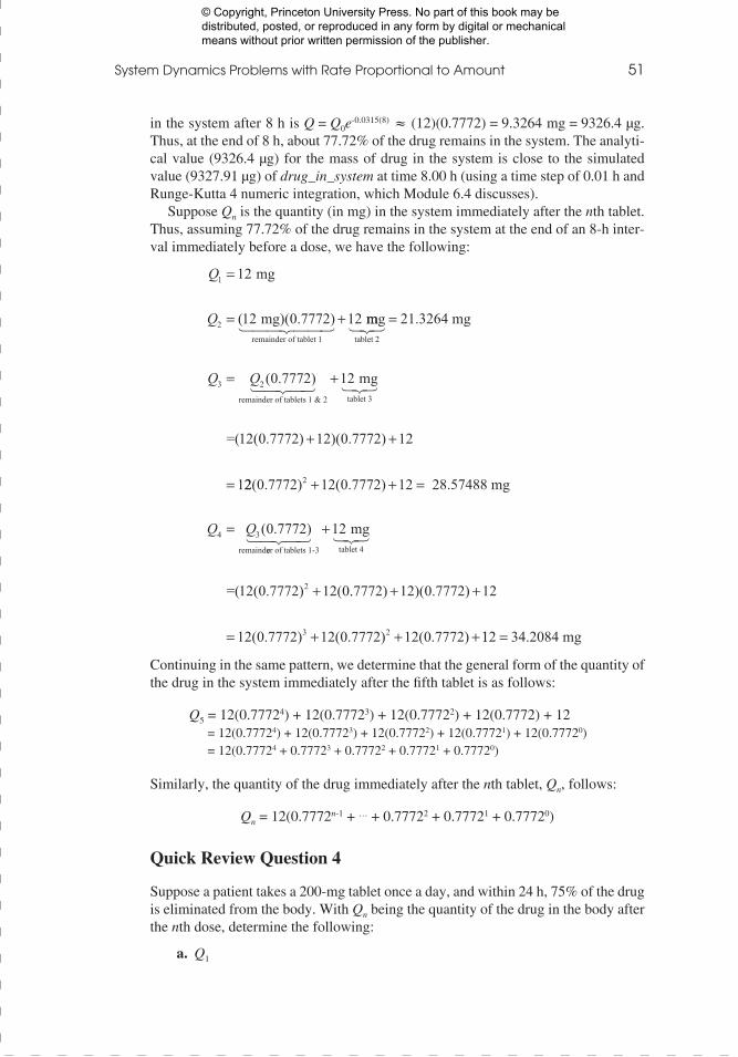
System Dynamics Problems with Rate Proportional to Amount 51
in the system after 8 h is Q = Q0e-0.0315(8) ≈ (12)(0.7772) = 9.3264 mg = 9326.4 µg.
Thus, at the end of 8 h, about 77.72% of the drug remains in the system. The analyti-cal value (9326.4 µg) for the mass of drug in the system is close to the simulated value (9327.91 µg) of drug_in_system at time 8.00 h (using a time step of 0.01 h and Runge-Kutta 4 numeric integration, which Module 6.4 discusses).
Suppose Qn is the quantity (in mg) in the system immediately after the nth tablet. Thus, assuming 77.72% of the drug remains in the system at the end of an 8-h inter-val immediately before a dose, we have the following:
Continuing in the same pattern, we determine that the general form of the quantity of the drug in the system immediately after the fifth tablet is as follows:
Q5 = 12(0.77724) + 12(0.77723) + 12(0.77722) + 12(0.7772) + 12 = 12(0.77724) + 12(0.77723) + 12(0.77722) + 12(0.77721) + 12(0.77720) = 12(0.77724 + 0.77723 + 0.77722 + 0.77721 + 0.77720)
Similarly, the quantity of the drug immediately after the nth tablet, Qn, follows:
Qn = 12(0.7772n-1 + … + 0.77722 + 0.77721 + 0.77720)
Quick Review Question 4
Suppose a patient takes a 200-mg tablet once a day, and within 24 h, 75% of the drug is eliminated from the body. With Qn being the quantity of the drug in the body after the nth dose, determine the following:
a. Q1
Q
Q
1
2
12
12 0 7772 12
=
= +
mg
mg) remainder of tablet 1
( ( . )� ��� ��� mmg 21.3264 mgtablet 2
remainder of tablets
��� =
=Q Q3 2 0 7772( . ) 1 & 2 tablet 3
mg
=( 2
� �� �� ���+
+ +
=
12
1 0 7772 12 0 7772 12
1
( . ) )( . )
22 0 7772 12 0 7772 12
0 7772
2
4 3
( . ) ( . )
( . )
+ + =
=
28.57488 mg
remaind
Q Qeer of tablets 1-3 tablet 4
mg
=( 2
� �� �� ���+
+
12
1 0 7772 12 02( . ) ( .. ) )( . )
( . ) ( . ) ( . )
7772 12 0 7772 12
12 0 7772 12 0 7772 12 0 77723 2
+ +
= + + +112 = 34.2084 mg
In order to view this proof accurately, the Overprint Preview Option must be checked in Acrobat Professional or Adobe Reader. Please contact your Customer Service Rep-
resentative if you have questions about finding the option.
Job Name: Cyan = PMS 300/356585t
© Copyright, Princeton University Press. No part of this book may be distributed, posted, or reproduced in any form by digital or mechanical means without prior written permission of the publisher.
52 Module 2.5
b. Q2 expressed as a sumc. Q3 expressed as a sumd. Q4 expressed as a sume. Qn expressed as a sum
We would like to determine what happens to the quantity of the drug in the sys-tem over a long period of time. To do so, we need a formula for the sum 0.7772n–1 + ∙ ∙ ∙ + 0.77722 + 0.77721 + 0.77720 for positive integer n. This sum is a finite geo-metric series, and its general form is as follows:
an–1 + ∙ ∙ ∙ + a2 + a1 + a0 for a ≠ 1 and positive integer n
As we verify in the next section, this sum is the following ratio:
an–1 + ∙ ∙ ∙ + a2 + a1 + a0 = 11−( )−( )aa
n
for a ≠ 1
Thus, for a = 0.7772 and n = 5, we can compute the value of Q5:
Q5 = 12(0.77724 + 0.77723 + 0.77722 + 0.77721 + 0.77720)
= 12 ⋅ −−
1 0 77721 0 7772
5..
= 38.5868 mg = 38,586.8 µg
Within simulation error, this value agrees with drug_in_system (38,580.92) after the fifth dose, at time 32.01 h. In general, the quantity of the drug immediately after the nth tablet, Qn, is as follows:
Qn = 12(0.7772n–1 + ∙ ∙ ∙ + 0.77722 + 0.77721 + 0.77720)
= 12 ⋅− ( )
−1 0 7772
1 0 7772..
n
Quick Review Question 5
Using the drug of Quick Review Question 4 and the formula for the sum of a finite geometric series, evaluate the following:
a. Q10
b. Qn
Using the formula for the sum of a finite geometric series, we can compute the quantity of drug after the nth tablet. To determine the long-range affect, we let n go to infinity and see that Qn approaches 53.8599 mg, as follows:
Definition an–1 + ∙ ∙ ∙ + a2 + a1 + a0 for a ≠ 1 and positive integer n is a fi-nite geometric series with base a.
In order to view this proof accurately, the Overprint Preview Option must be checked in Acrobat Professional or Adobe Reader. Please contact your Customer Service Rep-
resentative if you have questions about finding the option.
Job Name: Cyan = PMS 300/356585t
© Copyright, Princeton University Press. No part of this book may be distributed, posted, or reproduced in any form by digital or mechanical means without prior written permission of the publisher.
System Dynamics Problems with Rate Proportional to Amount 53
Qn = 121 0 7772
1 0 777212 1 0
1 0 7772⋅
− ( )−
→ ⋅ −−
≈.. .
n
53.8599 mg
Thus, the serum concentration is about (53.8599 mg)/(3000 mL) = 0.0179533 mg/mL = 17.95 µg/mL, which agrees closely with the peak value of the concentration in Figure 2.5.4.
Quick Review Question 6
Using the drug of Quick Review Questions 4 and 5, determine the quantity of drug after the nth tablet when the patient has been taking the drug for a long time.
Sum of Finite Geometric Series
To derive the formula for the sum of a finite geometric series, we start by consider-ing a particular example, Q5 as before. Let s be equal to the sum of the powers from 0 through 4 of 0.7772, as follows:
s = 0.77724 + 0.77723 + 0.77722 + 0.77721 + 0.77720 (1)
Multiplying both sides by 0.7772, we have the following:
0.7772s = (0.7772) (0.77724 + 0.77723 + 0.77722 + 0.77721 + 0.77720) 0.7772s = 0.77725 + 0.77724 + 0.77723 + 0.77722 + 0.77721 (2)
Subtracting Equation 2 from Equation 1, we subtract off all but two terms on the right:
s = 0.77724 + 0.77723 + 0.77722 + 0.77721 + 0.77720
−0.7772s = − 0.77725 − 0.77724 − 0.77723 − 0.77722 − 0.77721
s − 0.7772s = − 0.77725 + 0.77720
With 0.77720 being 1, we factor out s on the left as follows:
s(1 – 0.7772) = –0.77725 + 1
or
s(1 – 0.7772) = 1 – 0.77725
Dividing both sides by the factor (1 – 0.7772), we obtain the following formula:
s = 1 0 77721 0 7772
5−−
..
By the same reasoning, we have the general formula for the sum of a finite geometric series.
In order to view this proof accurately, the Overprint Preview Option must be checked in Acrobat Professional or Adobe Reader. Please contact your Customer Service Rep-
resentative if you have questions about finding the option.
Job Name: Cyan = PMS 300/356585t
© Copyright, Princeton University Press. No part of this book may be distributed, posted, or reproduced in any form by digital or mechanical means without prior written permission of the publisher.
54 Module 2.5
Two-Compartment Model
The one-compartment model is more appropriate for an injection of a drug into the system than for a pill, which takes time to dissolve, be absorbed, and be distributed within the system. In such cases, a two-compartment model might yield better re-sults. The first compartment represents the digestive system (stomach and/or intes-tines), while the second might indicate the blood, plasma, serum, or a particular organ that the drug targets. A flow pumps the drug from one compartment to the other in the model. One option for modeling the rate of change of absorption from the intestines to blood serum has the rate proportional to the amount of drug in the intestines. Probably a more accurate representation has the rate of change of absorp-tion from the intestines to blood serum be proportional to the volume of the intes-tines and to the difference of the drug concentrations in the intestines and serum.
Although the one- or two-compartment model is appropriate for most situations, a drug dosage problem could benefit from more compartments in a multicompart-ment model. Various projects employ more than one compartment.
Quick Review Question 7
This question applies to the rate of change of absorption of a drug from the intestines to blood serum in a two-compartment model. Suppose k is a constant of proportion-ality; i and b are the masses of the drug in the intestines and blood serum, respec-tively; vi and vb are the volumes of the intestines and blood serum, respectively; ci and cb are the drug concentrations in the stomach and blood serum, respectively; and time t is in hours.
a. Give the differential equation for this rate if the rate of absorption is propor-tional to the mass of drug in the intestines.
b. In this case, give the units of k.c. Give the differential equation for this rate if the rate of absorption is propor-
tional to the volume of the intestines and to the difference of the drug con-centrations in the intestines and blood serum.
d. In this case, give the units of k.
Exercises
1. Assuming that a quantity of a drug (Q) is Q = Q0eKt, show that K = –ln(0.5)/
t1/2, where t1/2 is the drug’s half-life.2. a. In Figure 2.5.4, what are the units for MEC and MTC?
The formula for the sum of a finite geometric series is as follows:
an–1 + ∙ ∙ ∙ + a2 + a1 + a0 = 11−( )−( )aa
n
for a ≠ 1
In order to view this proof accurately, the Overprint Preview Option must be checked in Acrobat Professional or Adobe Reader. Please contact your Customer Service Rep-
resentative if you have questions about finding the option.
Job Name: Cyan = PMS 300/356585t
© Copyright, Princeton University Press. No part of this book may be distributed, posted, or reproduced in any form by digital or mechanical means without prior written permission of the publisher.
System Dynamics Problems with Rate Proportional to Amount 55
b. What are the units for dosage? c. With a dosage of Dilantin being 100 mg, why is the value of dosage 100 *
1000?3. Prove the general formula for the sum of a finite geometric series.4. a. In Dilantin example, describe the effect a longer half-life has on
elimination_constant. b. Evaluate elimination_constant for t1/2 = 7 h. c. Evaluate elimination_constant for t1/2 = 22 h. d. Evaluate elimination_constant for t1/2 = 42 h.5. a. Suppose a patient taking Dilantin decides for convenience to take 300 mg
once a day instead of 100 mg every 8 h. Adjusting the model in OneCom-partDilantin, determine the results of such a decision. Is the decision advisable?
b. Mathematically, determine the long-term value of Qn, the quantity of Di-lantin in the system immediately after the nth dose, assuming absorption of only (0.09)(300 mg).
6. a. Determine mathematically the quantity of Dilantin in the system immedi-ately before the fifth dose. Use the same assumptions as in the section “Mathematics of Repeated Doses.”
b. Determine mathematically the long-term value of the quantity of Dilantin in the system immediately before the nth dose.
c. Compare your answers to the values in OneCompartDilantin.7. How should the one-dose aspirin example be adjusted to incorporate the
weight of a male patient? About 65% to 70% of a male’s body is liquid. As-sume that 1 kilogram (kg) of body liquid has a volume of 1 L. Assume the patient has a mass of 90 kg (comparable to about 198 lb).
Projects
For additional projects, see Module 7.7, “Cardiovascular System—A Pressure-Filled Model.”
1. Develop a two-compartment model for one dose of aspirin. 2. Develop a two-compartment model for aspirin, where someone with a
headache takes three aspirin tablets and 2 h later takes two more aspirin tablets.
3. In attempt to raise the concentration of a drug in the system to the minimum effective concentration quickly, sometimes doctors give a patient a loading dose, which is an initial dosage that is much higher than the maintenance dosage. A loading dose for Dilantin is three doses—400 mg, 300 mg, and 300 mg 2 h apart. Twenty-four hours after the loading dose, normal dosage of 100 mg every 8 h begins. Develop a model for this dosage regime.
4. Develop a two-compartment model for Dilantin, where the rate of change of absorption from the stomach to the blood serum is proportional to the amount of drug in the stomach.
5. Develop a two-compartment model for Dilantin, where the rate of change of absorption from the stomach to the blood serum is proportional to the
In order to view this proof accurately, the Overprint Preview Option must be checked in Acrobat Professional or Adobe Reader. Please contact your Customer Service Rep-
resentative if you have questions about finding the option.
Job Name: Cyan = PMS 300/356585t
© Copyright, Princeton University Press. No part of this book may be distributed, posted, or reproduced in any form by digital or mechanical means without prior written permission of the publisher.
56 Module 2.5
volume of the stomach and to the difference of the drug concentrations in the stomach and serum. Assume the volume of the stomach is 500 mL.
6. Develop a two-compartment model for a pediatric dosage of Dilantin that includes the mass of the patient. The initial dose is 5 mg/kg per day in two or three equally divided doses. The maintenance dosage is usually 4 to 8 mg/kg per day.
7. Develop a model for vancomycin HCI, which is a treatment for serious in-fections by susceptible strains of methicillin-resistant staphylococci in pen-icillin-allergic patients. The drug is administered by IV infusion. The intra-venous dose is usually 2 g divided either as 500 mg every 6 h or 1 g every 12 h, and the rate is no more than 10 mg/min or over a period of at least 50 min, whichever is longer. When kidney function is normal, multiple intra-venous dosing of 1 g results in mean plasma concentrations of about 63 µg/mL immediately after infusion, 23 µg/mL in 2 h, and 8 µg/mL 11 h after infusion. In such patients, the mean elimination half-life from plasma is 4 to 6 h. The mean plasma clearance is approximately 0.058 L/kg/h (liter of drug per kilogram of patient mass each hour), while the mean renal clear-ance is about 0.048 L/kg/h (Hospira 2010). Thus, include the mass of the patient in the model.
8. Repeat Project 7 for patients with renal dysfunction in which the average half-life of elimination is 7.5 da (Hospira 2010).
9. Develop a model for Vancocin HCI in which the patient initially has nor-mal kidney function (see Project 7). However, at the start of the third day, one of the patient’s kidneys stops functioning; and the elimination rate be-comes half its previous value. Consider using a step function.
10. Do Project 7 for children, where the dosage is 10 mg/kg every 6 h, and the rate of administration is over a period of at least 60 min (Hospira 2010).
11. Do Project 7 for neonates and young infants. The initial dose is 15 mg/kg. Thereafter, the dosage is 10 mg/kg every 12 h for neonates in their first week of life and afterward, up to age of 1 mo, every 8 h. Administration is more than 60 min (Hospira 2010).
12. Model drug dosage of aspirin for arthritis, where the initial dose is 3 g/da in divided doses. The dosage can be increased. Relief usually occurs at plasma levels of 20 to 30 mg per 100 mL. The plasma half-life of aspirin increases with dosage, so that a dose of 1 g has a half-life of about 5 h and a dose of 2 g has a half-life of about 9 h.
13. Considering the information about mass in Project 7, do any of the previous projects except one involving children or infants, accounting for the mass of a male patient.
14. By consulting a pharmacy reference or website, such as http://www.nlm.nih.gov/medlineplus/druginformation.html, obtain relevant information about some drug. Model the dosage of this drug.
Answers to Quick Review Questions
1. K = –ln(0.5)/3.2 per hour = 0.22/h2. plasma_concentration = aspirin_in_plasma / plasma_volume
In order to view this proof accurately, the Overprint Preview Option must be checked in Acrobat Professional or Adobe Reader. Please contact your Customer Service Rep-
resentative if you have questions about finding the option.
Job Name: Cyan = PMS 300/356585t
© Copyright, Princeton University Press. No part of this book may be distributed, posted, or reproduced in any form by digital or mechanical means without prior written permission of the publisher.
System Dynamics Problems with Rate Proportional to Amount 57
3. absorption_fraction * (pulse of amount dosage beginning at start every in-terval hours), where the pulse function depends on the particular system dy-namics tool
4. a. 200 mg b. (200 mg)(0.25) + 200 mg c. (200 mg)(0.25)2 + (200 mg)(0.25) + 200 mg d. (200 mg)(0.25)3 + (200 mg)(0.25)2 + (200 mg)(0.25) + 200 mg e. (200 mg)(0.25)n-1 + ∙ ∙ ∙ + (200 mg)(0.25)2 + (200 mg)(0.25) + 200 mg5. a. (200 mg)(1 – (0.25)10)/(1 – 0.25) = 266.67 mg b. (200 mg)(1 – (0.25)n)/(1 – 0.25) = (200 mg)(1 – (0.25)n)/(0.75) 6. (200 mg)(1 – 0)/(0.75) = 266.67 mg 7. a. db/dt = ki b. 1/h c. db/dt = k(vi)(ci – cb) d. 1/h
References
Ellis, Janice Rider, and Celia Love Hartley. 2004. Nursing in Today’s World: Trends, Issues & Management. Philadelphia: Lippincott, Williams and Wilkins.
Fitzgerald, Walter L., Jr., and Dennis B. Wilson. 1998. “Medication Errors: Lessons in Law.” Drug Topics, January 19, 1998. Hospital Pharmacy Reporter. February 1998.
Hospira. 2010. “Vancomycin Hydrochloride for Injection, USP.” Package insert. http://www.hospira.com/Images/EN-2613_32-5771_1.pdf (accessed December 30, 2012)
IOM (Institute of Medicine). 2007. Committee on Identifying and Preventing Medi-cation Errors. Preventing Medication Errors: Quality Chasm Series. Philip Asp-den, Julie Wolcott, J. Lyle Bootman, Linda R. Cronenwett, eds.
Khorasheh, Farhad, Amir Mahbod Ahmadi, and Abbas Gerayeli. 1999. “Application of Direct Search Optimization for Pharmacokinetic Parameter Estimation.” J Pharm Pharmaceutical Science 2(3): 92–98. http://www.ualberta.ca/~csps/JPPS2(3) /F.Khorasheh/application.htm (accessed December 18, 2012)
NQF (National Quality Forum). 2010. “Preventing Medication Errors: A $21 Bil-lion Opportunity.” http://www.qualityforum.org/Publications/2010/12/Prevent ing_Medication_Errors_CAB.aspx
Patel, A., and B. Ross. 2010. “Walgreens Told to Pay $25.8 Million Over Teen Phar-macy Tech’s Error.” The Blotter. ABC News. http://abcnews.go.com/Blotter/walgreens-told-pay-285-mil-teen-pharmacy-techs/story?id=9977262# .UJXKrI7et38 (accessed October 20, 2012)
Pharmacy Network Group. “Pharmacy Network Group Home Page.” http://www .pharmacynetworkgroup.com/ (accessed December 18, 2012)
Robert, Teri. 2004. “Teenager Dies from Acetaminophen Overdose.” Your Guide to Headaches/Migraine, About, Inc. http://headaches.about.com/cs/medication susage/a/acet_death.htm. (accessed December 18, 2012) Source for this Web ar-ticle: “Teenager Accidentally Overdoses on Over-the-Counter Analgesic,” July 2, 2003. http://TheAssociatedPress.ChannelOklahoma.com
In order to view this proof accurately, the Overprint Preview Option must be checked in Acrobat Professional or Adobe Reader. Please contact your Customer Service Rep-
resentative if you have questions about finding the option.
Job Name: Cyan = PMS 300/356585t
© Copyright, Princeton University Press. No part of this book may be distributed, posted, or reproduced in any form by digital or mechanical means without prior written permission of the publisher.