Technical Model DY Vortex Information Flowmeter

Yokogawa Electric Corporation

TechnicalInformation

<Int> <Ind> <Rev>

Model DY VortexFlowmeter

TI 01F06A00-01E

TI 01F06A00-01E© Copyright May 20011st Edition May 2001

Blank Page

Toc-1<Int> <Ind> <Rev>

TI 01F06A00-01E

Model DY Vortex Flowmeter

CONTENTS

1st Edition : May 30, 2001-00

TI 01F06A00-01E 1st Edition

1. PREFACE .................................................................................................... 1-1

2. FEATURES .................................................................................................. 2-12.1 Features of Vortex Flowmeter ................................................................................. 2-1

2.2 Unique Features of digitalYEWFLO........................................................................ 2-1

2.2.1 Features of Sensor Section ..................................................................... 2-1

2.2.2 Features of Converters ............................................................................ 2-2

3. PRINCPLE OF MEASUREMENT ................................................................. 3-1

4. METHOD OF DETECTING VORTEX-SHEDDING FREQUENCY ................. 4-14.1 Principle of Frequency Detection .......................................................................... 4-2

4.2 Principle of Operation ............................................................................................. 4-3

4.2.1 Detector Construction .............................................................................. 4-3

4.2.2 Spectral Signal Processing (SSP) ........................................................... 4-4

5. FLOW RATE CALCULATION ...................................................................... 5-1

6. CORRECTION FUNCTIONS........................................................................ 6-16.1 Reynolds Number Correction ................................................................................. 6-1

6.2 Compressibility Coefficient Correction ................................................................. 6-1

7. SELF-DIAGNOSIS FUNCTION .................................................................... 7-1

8. BASIC DATA ................................................................................................ 8-18.1 Effects of Spectral Adaptive Filter .......................................................................... 8-1

8.2 Effects of Adaptive Noise Suppression ................................................................. 8-3

8.3 Measurement in Low Flow Rate .............................................................................. 8-5

9. SIZING ......................................................................................................... 9-1

10. FLUID DATA .............................................................................................. 10-1

../../index.htm

Blank Page

<Toc> <Ind> <1. PREFACE> 1-1

TI 01F06A00-01E 1st Edition : May 30, 2001-00

1. PREFACEGenerally, a blunt body (vortex shedder) submerged in a flowing fluid sheds theboundary-layer from its surface and generates alternating-whirl in the backwardstream called the Karman vortex street. The frequency of this vortex street isdirectly proportional to the flow velocity within a given range of Reynolds num-ber. Therefore, the flow velocity or flow rate can be measured by measuring thevortex-shedding frequency. Vortex flowmeters work on this principle.

Based on the sales of 200,000 flowmeters around the world and years of experi-ence since developing the world's first commercial vortex flowmeter in 1968,Yokogawa has now developed the digitalYEWFLO.

In addition to the reliability and endurance of former models, the digitalYEWFLOhas an on-board SSP amplifier based on the state-of-the-art digital circuit tech-nology to provide high-level stability and accuracy.

■ New Feature, Spectral Signal Processing (SSP) Amplifier

● Spectral Adaptive Filter (Key technology)

The spectral adaptive filter integrated in the DSP amplifier analyzes vortex signals so that theoptimum measuring condition can be obtained without any interaction.

● Adaptive noise Suppression (ANS)

Eliminates all possible effects from vibrations, allowing vortex signals to be received preciselyand ensuring stable signals, even under environments where piping vibrations inevitably occur.

● Multi-function display

The two-column display allows monitoring of the instantaneous flow rate and sum together. Italso displays piping vibrations or fluid fluctuations from the self-diagnostic, allowing for early-stage judgement and/or remedies in the field.

../submenu.htm

../../index.htm

Blank Page

<Toc> <Ind> <2. FEATURES> 2-1


2. FEATURESThe digital YEWFLO has many unique features in addition to the usual featuresof conventional vortex flowmeters.

2.1 Features of Vortex Flowmeter● High accuracy

The accuracy of the vortex flowmeter is ±1% (pulse output) of the indicated value for bothliquids and gases and is higher compared to orifice flowmeters. For liquids, an accuracy of±0.75% is available depending on the fluid types and their conditions.

● Wide rangeability

Rangeability is defined as the ratio of the maximum value to the minimum value of the measur-able range. Its broad rangeability allows YEWFLO to operate in processes where the measuringpoint may fluctuate greatly.

● Output is proportional to flow rate

Since the output is directly proportional to the flow rate (flow velocity), no square root calcula-tion is needed, while orifice flowmeters require square root calculation.

● No zero-point fluctuation

Since frequency is output from the sensor, zero-point shift does not occur.

● Minimal pressure loss

Since only the vortex shedder is placed in the pipe of the vortex flowmeter, the fluid pressureloss due to the small restriction in the flow piping is small compared with flowmeters having anorifice plate.

2.2 Unique Features of digitalYEWFLO

2.2.1 Features of Sensor Section

● Sensor is not exposed to process fluid

The digital YEWFLO uses piezoelectric elements for the sensor; these are embedded inside thevortex shedder and are not exposed to the process fluid.

● Simple construction with no moving parts

Only the vortex shedder with a trapezoidal cross section and no moving parts are placed in theflow piping. This gives the digital YEWFLO a solid and simple construction.

● Operable at high-temperature and high-pressure without any problem

The digital YEWFLO measures hot fluids up to 450°C (25 to 200 mm, HT remote convertertype for high temperature) and high-pressure fluids up to ANSI class 900 flange rating (15 MPaat ambient temperature) as standard.

../submenu.htm

../../index.htm

2-2<Toc> <Ind> <2. FEATURES>


● Low cost of ownership

Compared with other flowmeters, the total cost for YEWFLO (including installation and main-tenance cost) is very economical.

2.2.2 Features of Converters

■ New Functions with SSP (Spectral Signal Processing) TechnologySSP is built into the powerful electronics of digitalYEWFLO. SSP analyses the fluid conditionsinside digitalYEWFLO and uses the data to automatically select the optimum adjustment for theapplication, providing features never before seen in a vortex flowmeter.

SSP accurately senses vortices in the low flow range, providing outstanding flow stability.

● Adaptive noise suppression (ANS) technology

The full automation of adaptive noise suppression allows for the provision of optimal measure-ment conditions immediately after turning on the system. Even under environments wherepiping vibrations are inevitable, it can capture vortex signals without being influenced byvibrations to ensure stable output signals.

● Improved self-diagnosis

Improved self-diagnosis enables the detection and displaying of the influences from excessivepiping vibrations or fluid fluctuations at an early stage. This allows early determination of theline status.

● Improved operability for setting parameters

Frequently used parameters are grouped into one block to significantly improve the operability.

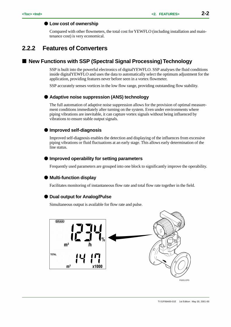
● Multi-function display

Facilitates monitoring of instantaneous flow rate and total flow rate together in the field.

● Dual output for Analog/Pulse

Simultaneous output is available for flow rate and pulse.

F0201.EPS

../submenu.htm

../../index.htm

<Toc> <Ind> <3. PRINCPLE OF MEASUREMENT> 3-1


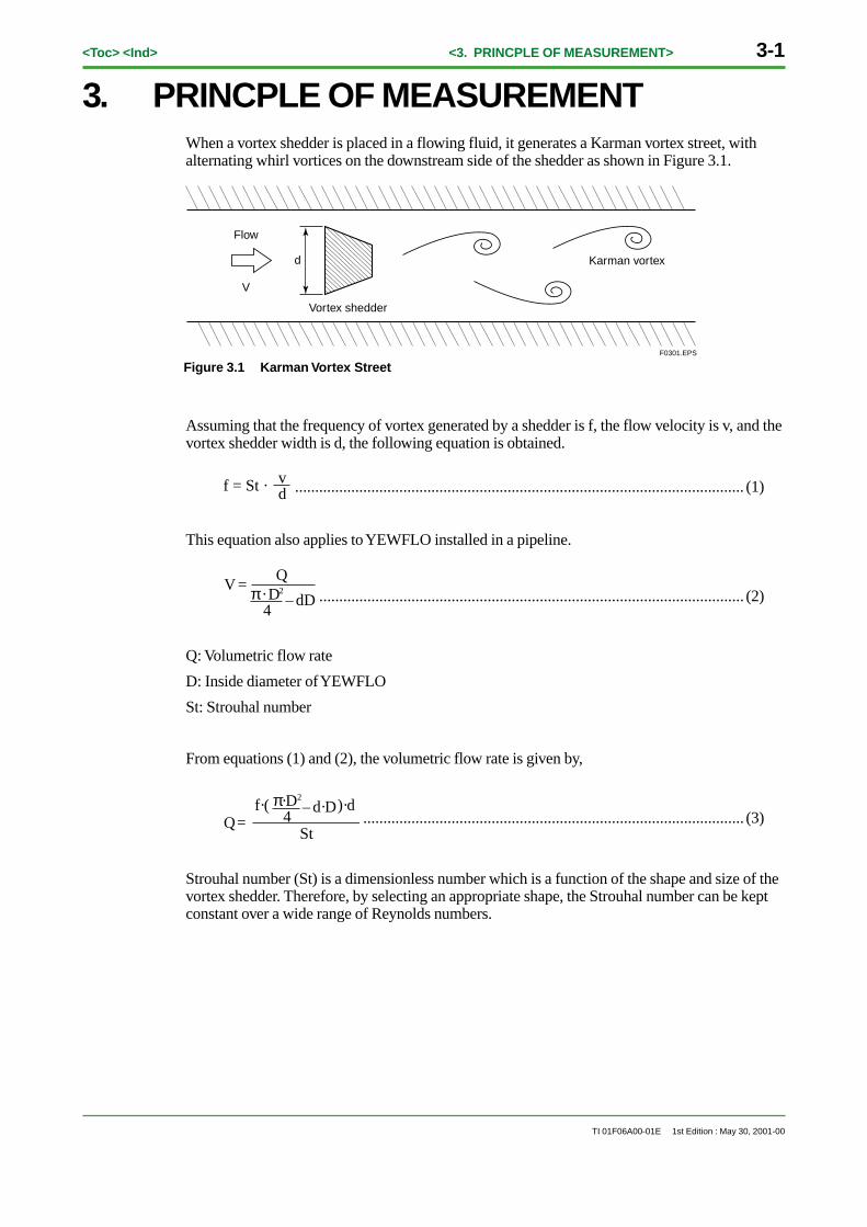
3. PRINCPLE OF MEASUREMENTWhen a vortex shedder is placed in a flowing fluid, it generates a Karman vortex street, withalternating whirl vortices on the downstream side of the shedder as shown in Figure 3.1.

Vortex shedder

Karman vortex

Flow

V

d

F0301.EPS

Figure 3.1 Karman Vortex Street

Assuming that the frequency of vortex generated by a shedder is f, the flow velocity is v, and thevortex shedder width is d, the following equation is obtained.

f = St · vd ................................................................................................................ (1)

This equation also applies to YEWFLO installed in a pipeline.

– dDV = π · D2

4

Q.......................................................................................................... (2)

Q: Volumetric flow rate

D: Inside diameter of YEWFLO

St: Strouhal number

From equations (1) and (2), the volumetric flow rate is given by,

– d·DQ=

f·( )·d

St

π·D2

4 ............................................................................................... (3)

Strouhal number (St) is a dimensionless number which is a function of the shape and size of thevortex shedder. Therefore, by selecting an appropriate shape, the Strouhal number can be keptconstant over a wide range of Reynolds numbers.

../submenu.htm

../../index.htm

3-2<Toc> <Ind> <3. PRINCPLE OF MEASUREMENT>


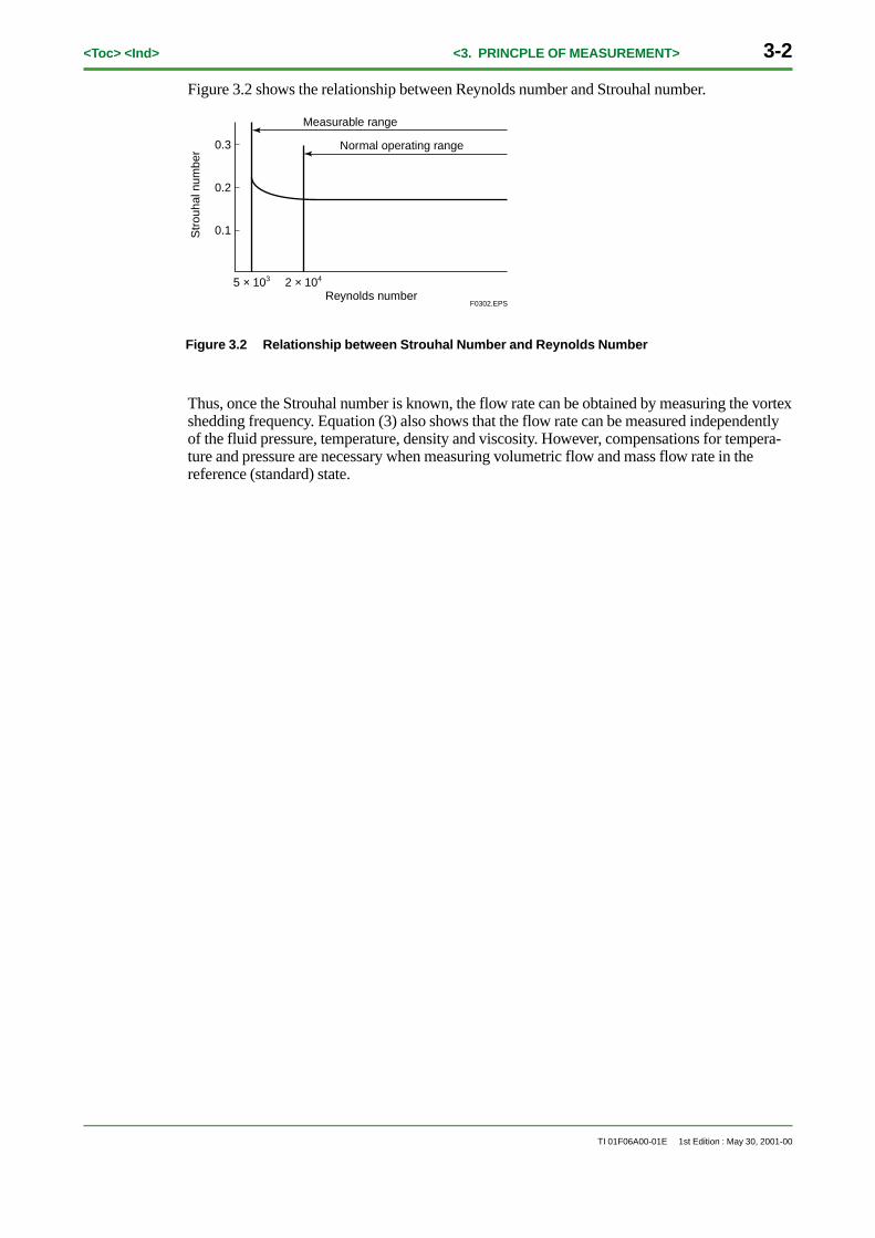
Figure 3.2 shows the relationship between Reynolds number and Strouhal number.

5 × 103 2 × 104

0.3

0.2

0.1Str

ouha

l num

ber

Reynolds number

Measurable range

Normal operating range

F0302.EPS

Figure 3.2 Relationship between Strouhal Number and Reynolds Number

Thus, once the Strouhal number is known, the flow rate can be obtained by measuring the vortexshedding frequency. Equation (3) also shows that the flow rate can be measured independentlyof the fluid pressure, temperature, density and viscosity. However, compensations for tempera-ture and pressure are necessary when measuring volumetric flow and mass flow rate in thereference (standard) state.

../submenu.htm

../../index.htm

<Toc> <Ind> <4. METHOD OF DETECTING VORTEX-SHEDDING FREQUENCY> 4-1


4. METHOD OF DETECTING VORTEX-SHEDDING FREQUENCY

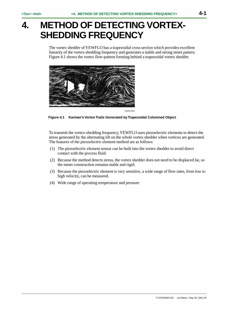
The vortex shedder of YEWFLO has a trapezoidal cross section which provides excellentlinearity of the vortex-shedding frequency and generates a stable and strong street pattern.Figure 4.1 shows the vortex flow-pattern forming behind a trapezoidal vortex shedder.

Figure 4.1 Karman’s Vortex Trails Generated by Trapezoidal Columned Object

To transmit the vortex-shedding frequency, YEWFLO uses piezoelectric elements to detect thestress generated by the alternating lift on the whole vortex shedder when vortices are generated.The features of the piezoelectric element method are as follows:

(1) The piezoelectric element sensor can be built into the vortex shedder to avoid directcontact with the process fluid.

(2) Because the method detects stress, the vortex shedder does not need to be displaced far, sothe meter construction remains stable and rigid.

(3) Because the piezoelectric element is very sensitive, a wide range of flow rates, from low tohigh velocity, can be measured.

(4) Wide range of operating temperature and pressure

F0401.EPS

../submenu.htm

../../index.htm

4-2<Toc> <Ind> <4. METHOD OF DETECTING VORTEX-SHEDDING FREQUENCY>


4.1 Principle of Frequency Detection

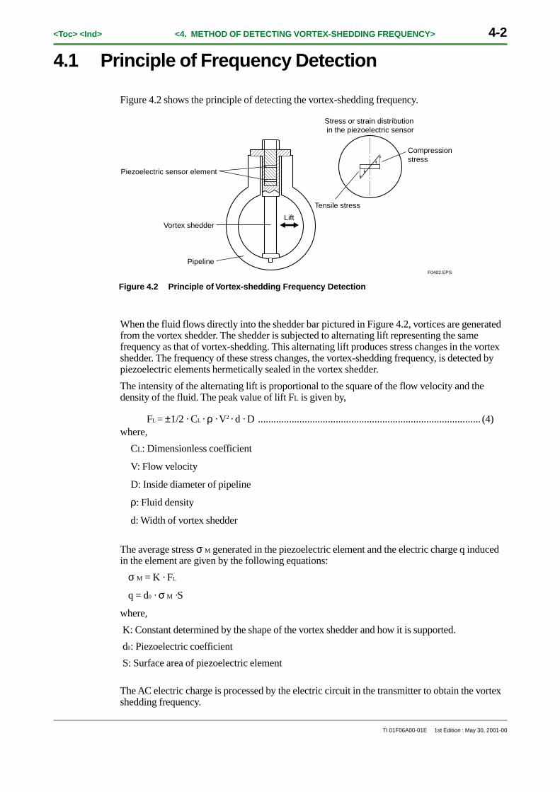
Figure 4.2 shows the principle of detecting the vortex-shedding frequency.

Stress or strain distribution in the piezoelectric sensor

Piezoelectric sensor element

Vortex shedder

Pipeline

Compression stress

Tensile stress

Lift

F0402.EPS

Figure 4.2 Principle of Vortex-shedding Frequency Detection

When the fluid flows directly into the shedder bar pictured in Figure 4.2, vortices are generatedfrom the vortex shedder. The shedder is subjected to alternating lift representing the samefrequency as that of vortex-shedding. This alternating lift produces stress changes in the vortexshedder. The frequency of these stress changes, the vortex-shedding frequency, is detected bypiezoelectric elements hermetically sealed in the vortex shedder.

The intensity of the alternating lift is proportional to the square of the flow velocity and thedensity of the fluid. The peak value of lift FL is given by,

FL = ±1/2 · CL · ρ · V2 · d · D ...................................................................................... (4)where,

CL: Dimensionless coefficient

V: Flow velocity

D: Inside diameter of pipeline

ρ: Fluid density

d: Width of vortex shedder

The average stress σ M generated in the piezoelectric element and the electric charge q inducedin the element are given by the following equations:

σ M = K · FL

q = d0 · σ M ·S

where,

K: Constant determined by the shape of the vortex shedder and how it is supported.

d0: Piezoelectric coefficient

S: Surface area of piezoelectric element

The AC electric charge is processed by the electric circuit in the transmitter to obtain the vortexshedding frequency.

../submenu.htm

../../index.htm



4.2 Principle of Operation

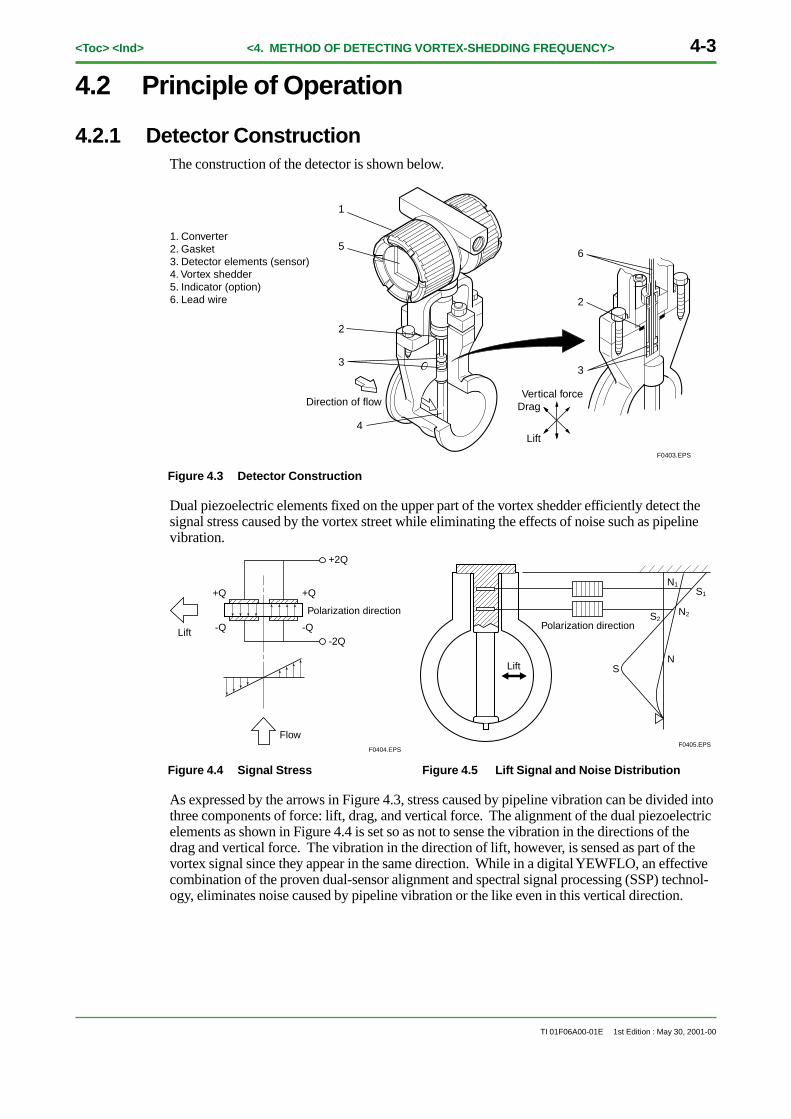
4.2.1 Detector ConstructionThe construction of the detector is shown below.

6

1

5

2

3

4

2

3

1. Converter2. Gasket3. Detector elements (sensor)4. Vortex shedder5. Indicator (option)6. Lead wire

Direction of flow

F0403.EPS

Vertical forceDrag

Lift

Figure 4.3 Detector Construction

Dual piezoelectric elements fixed on the upper part of the vortex shedder efficiently detect thesignal stress caused by the vortex street while eliminating the effects of noise such as pipelinevibration.

Lift

+Q

-Q

+Q

-Q

+2Q

-2Q

Polarization direction

FlowF0404.EPS

Lift

N1

N2

S1

S2

SN

Polarization direction

F0405.EPS

Figure 4.4 Signal Stress Figure 4.5 Lift Signal and Noise Distribution

As expressed by the arrows in Figure 4.3, stress caused by pipeline vibration can be divided intothree components of force: lift, drag, and vertical force. The alignment of the dual piezoelectricelements as shown in Figure 4.4 is set so as not to sense the vibration in the directions of thedrag and vertical force. The vibration in the direction of lift, however, is sensed as part of thevortex signal since they appear in the same direction. While in a digital YEWFLO, an effectivecombination of the proven dual-sensor alignment and spectral signal processing (SSP) technol-ogy, eliminates noise caused by pipeline vibration or the like even in this vertical direction.

../submenu.htm

../../index.htm



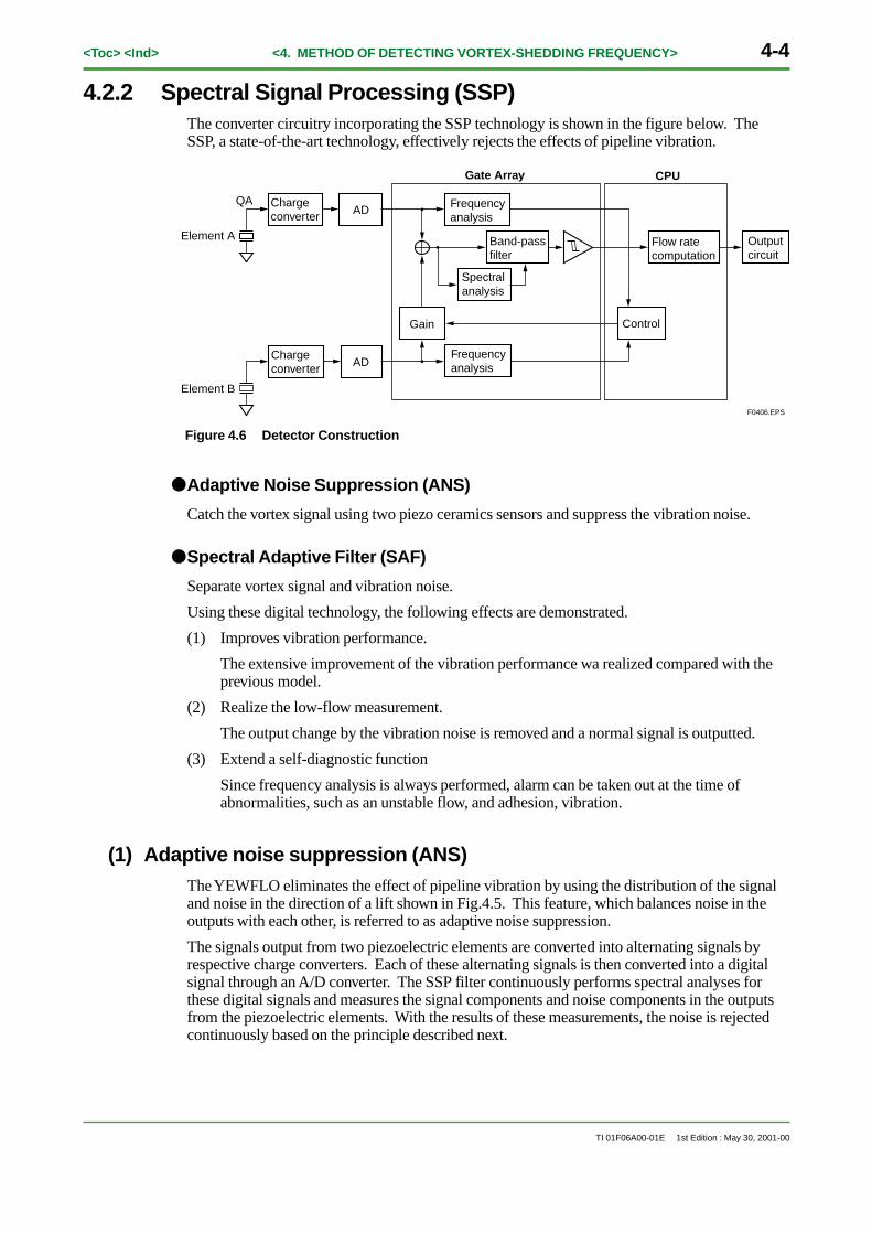
4.2.2 Spectral Signal Processing (SSP)The converter circuitry incorporating the SSP technology is shown in the figure below. TheSSP, a state-of-the-art technology, effectively rejects the effects of pipeline vibration.

Frequencyanalysis

F0406.EPS

Element A

Chargeconverter AD

QA

Control

Flow ratecomputation

Outputcircuit

AD

Gain

Band-passfilter

Element B

Gate Array CPU

Chargeconverter

Frequencyanalysis

Spectralanalysis

Figure 4.6 Detector Construction

● Adaptive Noise Suppression (ANS)

Catch the vortex signal using two piezo ceramics sensors and suppress the vibration noise.

● Spectral Adaptive Filter (SAF)

Separate vortex signal and vibration noise.

Using these digital technology, the following effects are demonstrated.

(1) Improves vibration performance.

The extensive improvement of the vibration performance wa realized compared with theprevious model.

(2) Realize the low-flow measurement.

The output change by the vibration noise is removed and a normal signal is outputted.

(3) Extend a self-diagnostic function

Since frequency analysis is always performed, alarm can be taken out at the time ofabnormalities, such as an unstable flow, and adhesion, vibration.

(1) Adaptive noise suppression (ANS)The YEWFLO eliminates the effect of pipeline vibration by using the distribution of the signaland noise in the direction of a lift shown in Fig.4.5. This feature, which balances noise in theoutputs with each other, is referred to as adaptive noise suppression.

The signals output from two piezoelectric elements are converted into alternating signals byrespective charge converters. Each of these alternating signals is then converted into a digitalsignal through an A/D converter. The SSP filter continuously performs spectral analyses forthese digital signals and measures the signal components and noise components in the outputsfrom the piezoelectric elements. With the results of these measurements, the noise is rejectedcontinuously based on the principle described next.

../submenu.htm

../../index.htm



QA QB

N1

QA = S1+N1

–QB = –S2–N2

QA–λQB = S1–λS2To SAF

FrequencyAnalysis

From the frequency analysis of QA and QB, it always calculates in CPU so that it may be set to N1 = λN2

From CPUVarying λ

Perform frequency analysis of a signal and a noise in each frequency band.

F0407.EPS

y6 y5 y4 y3 y2 y1

S1S1

N1 N1

S2

N2

Since the two piezoelectric elements, elements A and B, are so aligned as to be polarized inopposite directions, their outputs QA and QB can be expressed by the respective signal compo-nents S1 and S2, and noise components N1 and N2 as:

QA = S1 + N1 ............................................................................................................. (1)

–QB = –S2 – N2 .......................................................................................................... (2)

Multiplying the output of element B by a value (from 0.5 to 1.2), λ, obtains:

–λQB = –λS2 – λN2 .................................................................................................... (3)

Then, adding this multiplied signal to the output of element A, namely, adding equation (2) toequation (3) obtains:

QA – λQB = S1 – λS2 + N1 – λN2 ................................................................................ (4)

When N1 is equal to λN2, equation (4) becomes as follows and only the signal components canbe detected:

QA – λQB = S1 – λS2 .................................................................................................................................................................................... (5)

Hence, if the detector can measure the amplitudes of noise components, N1 and N2 and candetermine the value of λ to offset them, the noise in the direction of lift can be eliminated.

For earlier models, the N1 and N2 levels were measured and the value of λ was adjusted duringshipment preparations. Therefore, if the noise ratio has changed from the factory-set λ after theflowmeter in question is installed on site, the intended noise rejection result cannot be obtained.While in a digital YEWFLO, the CPU automatically computes the optimum value at all timesand sets it in λ, so the signal components can always be extracted no matter if the noise ratiochanges.

../submenu.htm

../../index.htm



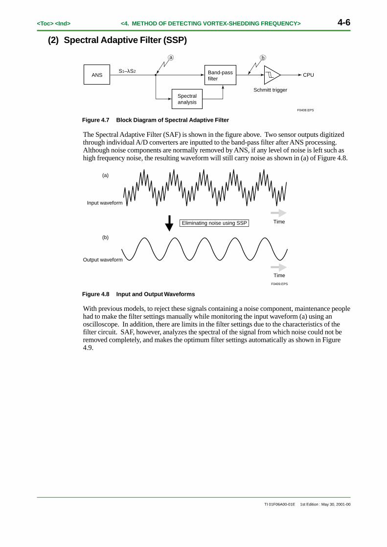
(2) Spectral Adaptive Filter (SSP)

Spectralanalysis

Band-passfilter

a b

Schmitt trigger

CPU

F0408.EPS

ANSS1–λS2

Figure 4.7 Block Diagram of Spectral Adaptive Filter

The Spectral Adaptive Filter (SAF) is shown in the figure above. Two sensor outputs digitizedthrough individual A/D converters are inputted to the band-pass filter after ANS processing.Although noise components are normally removed by ANS, if any level of noise is left such ashigh frequency noise, the resulting waveform will still carry noise as shown in (a) of Figure 4.8.

F0409.EPS

Input waveform

Output waveform

Eliminating noise using SSP Time

Time

(a)

(b)

Figure 4.8 Input and Output Waveforms

With previous models, to reject these signals containing a noise component, maintenance peoplehad to make the filter settings manually while monitoring the input waveform (a) using anoscilloscope. In addition, there are limits in the filter settings due to the characteristics of thefilter circuit. SAF, however, analyzes the spectral of the signal from which noise could not beremoved completely, and makes the optimum filter settings automatically as shown in Figure4.9.

../submenu.htm

../../index.htm



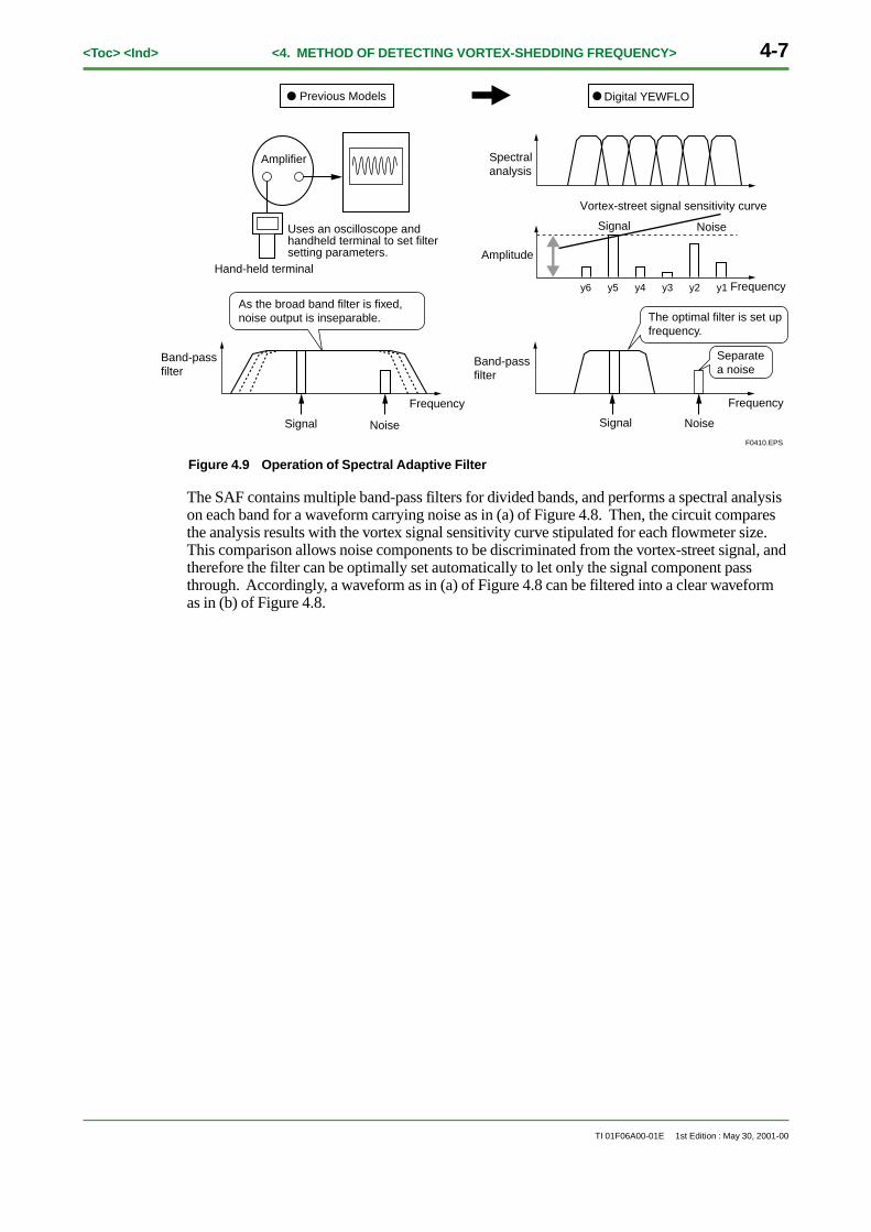
Previous Models Digital YEWFLO

Amplifier

Uses an oscilloscope and handheld terminal to set filter setting parameters.

Hand-held terminal

Band-pass filter

Signal Noise

Frequency

Band-passfilter

Amplitude

Spectral analysis

Signal Noise

Signal Noise

Frequency

Frequency

Vortex-street signal sensitivity curve

y6 y5 y4 y3 y2 y1

The optimal filter is set upfrequency.

As the broad band filter is fixed,noise output is inseparable.

F0410.EPS

Separate a noise

Figure 4.9 Operation of Spectral Adaptive Filter

The SAF contains multiple band-pass filters for divided bands, and performs a spectral analysison each band for a waveform carrying noise as in (a) of Figure 4.8. Then, the circuit comparesthe analysis results with the vortex signal sensitivity curve stipulated for each flowmeter size.This comparison allows noise components to be discriminated from the vortex-street signal, andtherefore the filter can be optimally set automatically to let only the signal component passthrough. Accordingly, a waveform as in (a) of Figure 4.8 can be filtered into a clear waveformas in (b) of Figure 4.8.

../submenu.htm

../../index.htm

Blank Page

<Toc> <Ind> <5. FLOW RATE CALCULATION> 5-1


5. FLOW RATE CALCULATIONThe flow rate is calculated based on the count number N of generated vortices as follows:

a) Flow rate (actual flow rate unit)

RATE = N• • UKT • UK • UTM • • εf • εe • εr • εp•1∆t

1KT

1SE

.................................... (8)

KT = KM • {1– 4.81×(Tf –15)×10-5} ........................................................................ (9)

b) Flow rate (%)

RATE (%) = RATE • 1FS

...................................................................................... (10)

c) Integrated value

For a scaled pulse

TOTAL = N • εf • εe • εr • εp • • UKT • UK • 1

KT1TE

.................................................. (11)

For an unscaled pulse

TOTAL = εf • εe • εr • εp • N ..................................................................................... (12)

d) Flow velocity

1∆t

1KT

4π•D2• UKT ••V= N• ............................................................................... (13)

e) Reynolds number

µpf

Red =V•D ×106

×1000 ....................................................................................... (14)

where,

N : Input pulse number (pulse)

εf : Correction coefficient of instrument error

εr : Correction coefficient of Reynolds number

εe : Correction coefficient of expansion for compressible fluid

εp : Correction coefficient of adjacent pipe

KM : K factor in 15°C (p/l)

KT : K factor for operating temperature (P/l)

UKT : Unit conversion coefficient of K factor

UTM : Coefficient for flow rate unit time (e.g.: /m (min) = 60)

SE : Span factor (ex.: E + 3 = 103)

../submenu.htm

../../index.htm

5-2<Toc> <Ind> <5. FLOW RATE CALCULATION>


FS : Flow rate span

µ : Viscosity coefficient (cP)

D : Internal diameter (m)

∆t : Time corresponding to N (second)

Uk : Flow conversion coefficient

Tf : Operating temperature (°C)

TE : Total factor

pf : Operating density (kg/m3)

The flow conversion coefficient Uk is automatically calculated just by setting parameters(temperature, pressure and density).

The parameters to be set are sequentially displayed on a hand held BT200 (BRAIN terminal)when the fluid type is specified.

../submenu.htm

../../index.htm

<Toc> <Ind> <6. CORRECTION FUNCTIONS> 6-1


6. CORRECTION FUNCTIONSThe digitalYEWFLO has extensive correction functions to support various appli-cations. These correction functions are outlined below.

6.1 Reynolds Number CorrectionIn a 3-dimensional flow inside a pipeline, as Reynolds number (≤20000) decreases, the Strouhalnumber (K factor) gradually increases. The curve of this K factor is corrected using a 5-pointline segment approximation.

0.17

0.160.5 1 2 5 10 20 50 × 104

0.18

0.19

0.20 Water

Fuel oil (specific gravity: 0.85)

0.2 MPa abs. Air

0.4 MPa abs. Air

0.6 MPa abs. Air

Air

Water

Fuel oil

Reynolds number (Re)F0601.EPS

Str

ouha

l num

ber

(St)

Figure 6.1 Strouhal Number for Low Reynolds Number

6.2 Compressibility Coefficient CorrectionPressure changes and errors are generated, as the compressible fluid flow becomes faster.Assuming that the fluid changes state adiabatically, the vortex-shedding frequency of thecompressible fluid is given by the following equation.

( )f = A · · St ·P1P2

V2

d

1/K.............................................................................................. (15)

where

V2 : Local average flow velocity at position 2.5D downstream of the vortex shedder

P1 : Pressure at position 1D upstream of the vortex shedder

κ : Ratio of specific heat of gas

A : Coefficient indicating the influence of flow velocity distribution and area ratio

P2 : Pressure at position 2.5D down stream of the vortex shedder

St : Strouhal number

d : Internal diameter

../submenu.htm

../../index.htm

6-2<Toc> <Ind> <6. CORRECTION FUNCTIONS>


P = 2.6MPa

P = 1.2MPa

P = 0.4MPa

5

±1%

1.434

1.448

1.462

1.476

10 20 50

Velocity (m/s)

K fa

ctor

(p/

)

An example of air flow in a 100mm diameter pipe

F0602.EPS

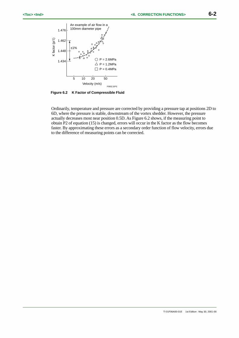
Figure 6.2 K Factor of Compressible Fluid

Ordinarily, temperature and pressure are corrected by providing a pressure tap at positions 2D to6D, where the pressure is stable, downstream of the vortex shedder. However, the pressureactually decreases most near position 0.5D. As Figure 6.2 shows, if the measuring point toobtain P2 of equation (15) is changed, errors will occur in the K factor as the flow becomesfaster. By approximating these errors as a secondary order function of flow velocity, errors dueto the difference of measuring points can be corrected.

../submenu.htm

../../index.htm

<Toc> <Ind> <7. SELF-DIAGNOSIS FUNCTION> 7-1


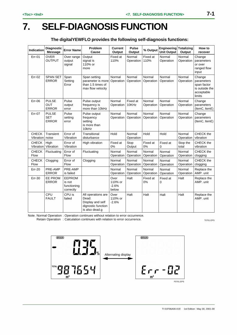
7. SELF-DIAGNOSIS FUNCTIONThe digitalYEWFLO provides the following self-diagnosis functions:

T0701.EPS

EngineeringUnit Output% Output

PulseOutput

CurrentOutput

ProblemCauseError Name

DiagnosticMessageIndication

Err-01

Err-02

Err-06

Err-07

CHECK Vibration CHECK Vibration CHECK Flow CHECK Flow Err-20

Err-30

OVER OUTPUT

SPAN SET ERROR

PULSE OUT ERROR PULSE SET ERROR

Transient noise High Vibration Fluctuating

Clogging

PRE-AMPERROR EE PROM ERROR

CPU FAULT

Over range output signal

Span Setting Error

Pulse output error Pulse setting error

Error of Vibration Error of Vibration Error of Flow Error of Flow PRE-AMPis failed EEPROM is not functioning correctly CPU is failed

Output signal is 110% or more

Span setting parameter is morethan 1.5 times of max flow velocity

Pulse output frequency is more than 10kHz Pulse output frequency setting is more than 10kHz Transitional disturbance High vibration

Fluctuating

Clogging

All operations are Dead.Display and self dignostic function is also dead.g

Fixed at 110%

Normal Operation

Normal Operation

Normal Operation

Hold

Fixed at 0% Normal Operation Normal Operation Normal Operation

Over 110% or -2.6% below Over110% or -2.6%

Normal Operation

Normal Operation

Fixed at 10KHz

Normal Operation

Normal Operation Stop Output Normal Operation Normal Operation Normal Operation Halt

Halt

Fixed at 110%

Normal Operation

Normal Operation

Normal Operation

Hold

Fixed at 0% Normal Operation Normal Operation Normal Operation Fixed at 0%

Halt

Normal Operation

Normal Operation

Normal Operation

Normal Operation

Hold

Fixed at 0 Normal Operation Normal Operation Normal Operation Fixed at 0

Halt

Normal Operation

Normal Operation

Normal Operation

Normal Operation

Normal Operation Stop the total Normal Operation Normal Operation Normal Operation Halt

Halt

Change parameters or over ranged flow input Change parameters span factor is outside the acceptable limits Change parameters(ItemC, ItemE) Change parameters(ItemC, ItemE)

CHECK the vibration CHECK the vibration CHECK the clogging CHECK the clogging Replace theAMP. unit Replace theAMP. unit

Replace theAMP. unit

TotalizingOutput

How torecover

Note. Normal Operation : Operation continues without relation to error occurrence.Retain Operation : Calculation continues with relation to error occurrence.

F0701.EPS

Alternating display

../submenu.htm

../../index.htm

Blank Page

<Toc> <Ind> <8. BASIC DATA> 8-1


8. BASIC DATA

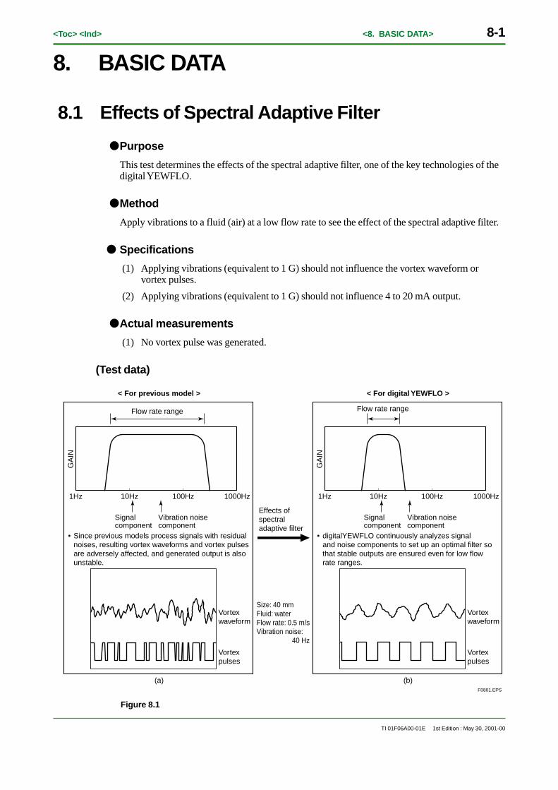
8.1 Effects of Spectral Adaptive Filter

● Purpose

This test determines the effects of the spectral adaptive filter, one of the key technologies of thedigital YEWFLO.

● Method

Apply vibrations to a fluid (air) at a low flow rate to see the effect of the spectral adaptive filter.

● Specifications

(1) Applying vibrations (equivalent to 1 G) should not influence the vortex waveform orvortex pulses.

(2) Applying vibrations (equivalent to 1 G) should not influence 4 to 20 mA output.

● Actual measurements

(1) No vortex pulse was generated.

(Test data)

Effects of spectral adaptive filter

Size: 40 mmFluid: waterFlow rate: 0.5 m/sVibration noise:

40 Hz

Flow rate range

1Hz 10Hz 100Hz 1000Hz

GA

IN

Signal component

Vibration noise component

Vortex waveform

Vortex pulses

• Since previous models process signals with residual noises, resulting vortex waveforms and vortex pulses are adversely affected, and generated output is also unstable.

Flow rate range

1Hz 10Hz 100Hz 1000Hz

GA

IN

Signal component

Vibration noise component

Vortex waveform

Vortex pulses

• digitalYEWFLO continuously analyzes signal and noise components to set up an optimal filter so that stable outputs are ensured even for low flow rate ranges.

< For previous model > < For digital YEWFLO >

(a) (b)F0801.EPS

Figure 8.1

../submenu.htm

../../index.htm

8-2<Toc> <Ind> <8. BASIC DATA>


(Description)

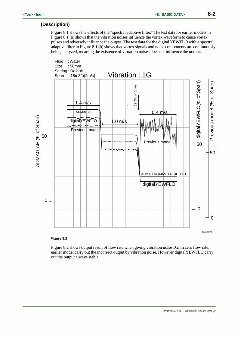
Figure 8.1 shows the effects of the “spectral adaptive filter.” The test data for earlier models inFigure 8.1 (a) shows that the vibration noises influence the vortex waveform to cause vortexpulses and adversely influence the output. The test data for the digital YEWFLO with a spectraladaptive filter in Figure 8.1 (b) shows that vortex signals and noise components are continuouslybeing analyzed, meaning the existence of vibration noises does not influence the output.

1.4 m/s

1.0 m/s

0.4 m/s

0

50

0

50

50

0

digi

talY

EW

FLO

(% o

f Spa

n)

Pre

viou

s m

odel

(%

of S

pan)

AD

MA

G A

E (

% o

f Spa

n)

ADMAG AE(MASTER METER)

digitalYEWFLO

ADMAG AE

digitalYEWFLO

Previous model

Fluid : WaterSize : 50mmSetting : DefaultSpan : 15m3/h(2m/s) Vibration : 1G

12.5

% o

f Spa

n

Previous model

F0802.EPS

Figure 8.2

Figure 8.2 shows output result of flow rate when giving vibration noise 1G. In zero flow rate,earlier model carry out the incorrect output by vibration noise. However digitalYEWFLO carryout the output always stable.

../submenu.htm

../../index.htm



8.2 Effects of Adaptive Noise Suppression

● Purpose

This test determines the effects of “auto noise balancing,” one of the key technologies of digitalYEWFLO.

● Method

Apply vibrations to a fluid (air) at zero flow rate to compare the auto noise balancing features ofan previous model and the digital YEWFLO.

● Specifications

(1) Applying vibrations (equivalent to 1 G) should not cause vortex pulses.

(2) Applying vibrations (equivalent to 1 G) should not influence 4 to 20 mA output.

● Actual measurements

(1) No vortex pulse was generated.

(2) No effect on the output was found.

(Test data)

Vortex waveform

Vortex pulses

100

200

300

400

Auto noise balance OFF(a)

Auto noise balance ON(b)

Error output: 25 m3/h Stable output: 0 m3/h

Vibration being applied

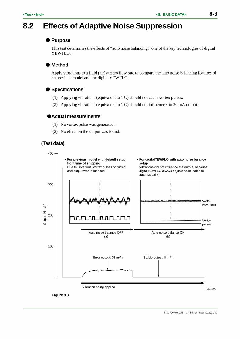
• For previous model with default setup from time of shippingDue to vibrations, vortex pulses occurred and output was influenced.

• For digitalYEWFLO with auto noise balance setupVibrations did not influence the output, because digitalYEWFLO always adjusts noise balance automatically.

Out

put [

Nm

3 /h]

F0803.EPS

Figure 8.3

../submenu.htm

../../index.htm

8-4<Toc> <Ind> <8. BASIC DATA>


(Description)

Figure 8.3 shows the effect of the auto noise balance. For the previous model in Figure 8.3 (a),the influences from vibration noises appeared on the vortex waveform, vortex pulses occurredand the output was influenced. Figure 8.3 (b) shows the effect of digitalYEWFLO with the autonoise balance turned on. The same noises which were applied to the previous model wereautomatically canceled, and no vortex pulse was generated. This means the vibrations did notinfluence the output.

../submenu.htm

../../index.htm



8.3 Measurement in Low Flow Rate

● Purpose

This test determines the effects of Low flow measurement comparing with previous model.

● Method

As compared with Magnetic Flowmeter (ADMAG AE), measurement of low flow rate isperformed conventionally.

(Test data)

0.2m/s0.22m/s0.24m/s0.26m/s0.28m/s0.3m/s0.32m/s

0.34m/s

ADMAG AE(MASTER METER)

digitalYEWFLO

Previous model

0

0

0

digi

talY

EW

FLO

(% o

f S

pan)

AD

MA

G A

E (

% o

f S

pan)

Fluid : WaterSize :50mm Setting : Default

2min

Pre

viou

s m

odel

(%

of

Spa

n)

25

25

25

F0804.EPS

Figure8.4

(Description)

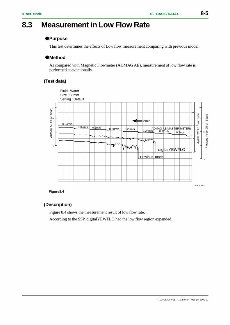
Figure 8.4 shows the measurement result of low flow rate.

According to the SSP, digitalYEWFLO had the low flow region expanded.

../submenu.htm

../../index.htm

Blank Page

<Toc> <Ind> <9. SIZING> 9-1


9. SIZINGThis section outlines the sizing for various fluids for check purposes. For detailson sizing, refer to GS 01F6A00-01E.

(1) Liquid

● Maximum measurable flow rate check

Table 9.1 Maximum Measurable Flow Rate Range for Each Flowmeter Size

Nominal diameter

Maximum measurable range [m3/h]

1/2 in. (15 mm)

6

1 in. (25 mm)

18

1.5 in. (40 mm)

44

2 in. (50 mm)

73

3 in. (80 mm)

142

4 in. (100 mm)

248

6 in. (150 mm)

544

8 in. (200 mm)

973

10 in. (250 mm)

1506

12 in. (300 mm)

2156

T0901.EPS

Maximum measurable range [m3/h]

(1) With reference to 15°C, except for ammonia which references to -40°C

(2) Maximum flow rate was calculated from a flow rate of 10 m/s.

● Minimum measurable flow rate check

Table 9.2 Minimum Measurable Flow Rate Ranges for Various Liquids

Water (H2O)

Methanol (CH3OH)

Ethanol (C2H5O)

Aniline (C6H5N)

Acetone (CH3)

Carbon bisulfide (CS2)

Carbon tetrachloride (CCl4)

Ammonia (NH3)

0.3

0.4

0.5

0.8

0.34

0.26

0.24

0.34

0.65

0.7

0.9

1.5

0.73

0.58

0.51

0.74

1.3

1.5

1.5

2.4

1.5

1.2

1.1

1.5

2.2

2.5

2.5

3.1

2.5

2.0

1.8

2.5

4.3

4.8

4.8

4.3

4.7

3.8

3.4

4.8

7.5

8.4

8.4

7.3

8.3

6.6

5.9

8.4

17

18

18

16

18

15

13

18

34

38

38

33

38

30

27

37

60

67

67

59

67

54

48

65

86

97

97

85

96

77

68

93

Nominal diameter 1/2 in. (15 mm)Fluid type

1 in. (25 mm)

1.5 in. (40 mm)

2 in. (50 mm)

3 in. (80 mm)

Minimum measurable range [m3/h]

4 in. (100 mm)

6 in. (150 mm)

8 in. (200 mm)

10 in. (250 mm)

12 in. (300 mm)

T0902.EPS

(1) For sizes of 2 inches or less, the above table shows the lower limit of the normal operationrange.

● Cavitation check

When using a YEWFLO with the same nominal diameter as the process piping and the mini-mum flow rate during operation becomes lower than the lower limit of the measurable range,perform a cavitation check for a YEWFLO one or two sizes smaller than the process pipe. If it isconfirmed that this smaller YEWFLO may not cause cavitation, install it to the piping usingreducers.

Cavitation occurs when the flow line pressure is low and flow verosity is high during measure-ment, preventing correct measurement of flow rate. Please be sure to perform a cavitation check.

../submenu.htm

../../index.htm

9-2<Toc> <Ind> <9. SIZING>


(2) Pressure Loss and Cavitation

● Pressure loss

For water with a flow velocity of 10 m/sec, use 108 kPa (1.1 kgf/cm2)

For atmospheric pressure with a flow velocity of 80 m/sec, use 9 kPa (910 mmH2O)

The pressure loss can be obtained from the following equation:

∆P =108×10-5×ρ×V2 ........................................................................................... (1)

or

∆P =135× ρ × Q2

D4 .................................................................................................. (2)

where

∆P : Pressure loss (kgf/cm2)

ρ : Fluid density at operating conditions (kg/m3)

V : Flow velocity (m/s)

Q : Volumetric flow rate at operating conditions (m3/h)

D : Flowmeter tube inner dia. (mm)

Figure 9.1 shows a graph based on the above equation.

When the nominal size is within 15mm to 50mm and the adjacent pipe is Sch40, and when thenominal size is within 80mm to 300mm and the adjacent pipe is Sch80, pressure loss will beapprox. 10% smaller than the calculated value.

● Cavitation (minimum line pressure)

In liquid measurement, a low line pressure and high flow velocity condition can cause cavitationand measuring flow velocities may fail. Minimum line pressure causing no cavitation can beobtained from the following equation:

P = 2.7 × ∆P+1.3 × PO ............................................................................................... (3)

P : Downstream 2 to 7 D line pressure, from the flowmeter downstream side end surface[kPa abs {kgf/cm2 abs}]

∆P : Pressure loss [kPa{kgf/cm2}]

Po : Saturate vapor pressure of liquid at operating conditions [kPa abs {kgf/cm2 abs}]

../submenu.htm

../../index.htm



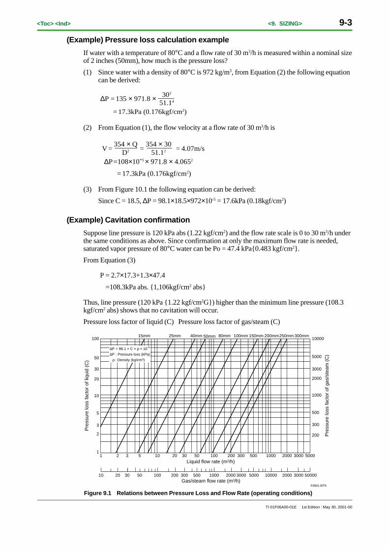
(Example) Pressure loss calculation example

If water with a temperature of 80°C and a flow rate of 30 m3/h is measured within a nominal sizeof 2 inches (50mm), how much is the pressure loss?

(1) Since water with a density of 80°C is 972 kg/m3, from Equation (2) the following equationcan be derived:

302

51.14∆P = 135 × 971.8 ×

= 17.3kPa (0.176kgf/cm2)

(2) From Equation (1), the flow velocity at a flow rate of 30 m3/h is

354 × QD2

354 × 3051.12V = = 4.07m/s =

= 17.3kPa (0.176kgf/cm2)

∆P=108×10-5 × 971.8 × 4.0652

(3) From Figure 10.1 the following equation can be derived:

Since C = 18.5, ∆P = 98.1×18.5×972×10-5 = 17.6kPa (0.18kgf/cm2)

(Example) Cavitation confirmation

Suppose line pressure is 120 kPa abs (1.22 kgf/cm2) and the flow rate scale is 0 to 30 m3/h underthe same conditions as above. Since confirmation at only the maximum flow rate is needed,saturated vapor pressure of 80°C water can be Po = 47.4 kPa{0.483 kgf/cm2}.

From Equation (3)

P = 2.7×17.3+1.3×47.4

=108.3kPa abs. {1,106kgf/cm2 abs}

Thus, line pressure (120 kPa {1.22 kgf/cm2G}) higher than the minimum line pressure (108.3kgf/cm2 abs) shows that no cavitation will occur.

Pressure loss factor of liquid (C) Pressure loss factor of gas/steam (C)

1 2 3 5 10 20 30 50 100 200 300 500 1000 2000 3000 5000

10 20 30 50 100 200 300 500 1000 2000 3000 5000 10000 2000 3000 50000

100

50

30

20

10

5

3

2

1

10000

5000

3000

2000

1000

500

300

200

Pre

ssur

e lo

ss fa

ctor

of l

iqui

d (C

)

Pre

ssur

e lo

ss fa

ctor

of g

as/s

team

(C

)

Gas/steam flow rate (m3/h)

Liquid flow rate (m3/h)

15mm 25mm 40mm 50mm 80mm 100mm 150mm 200mm250mm 300mm

∆P = 98.1 × C × ρ × 10-5

∆P : Pressure loss (kPa)

ρ : Density (kg/cm3)

F0901.EPS

Figure 9.1 Relations between Pressure Loss and Flow Rate (operating conditions)

../submenu.htm

../../index.htm



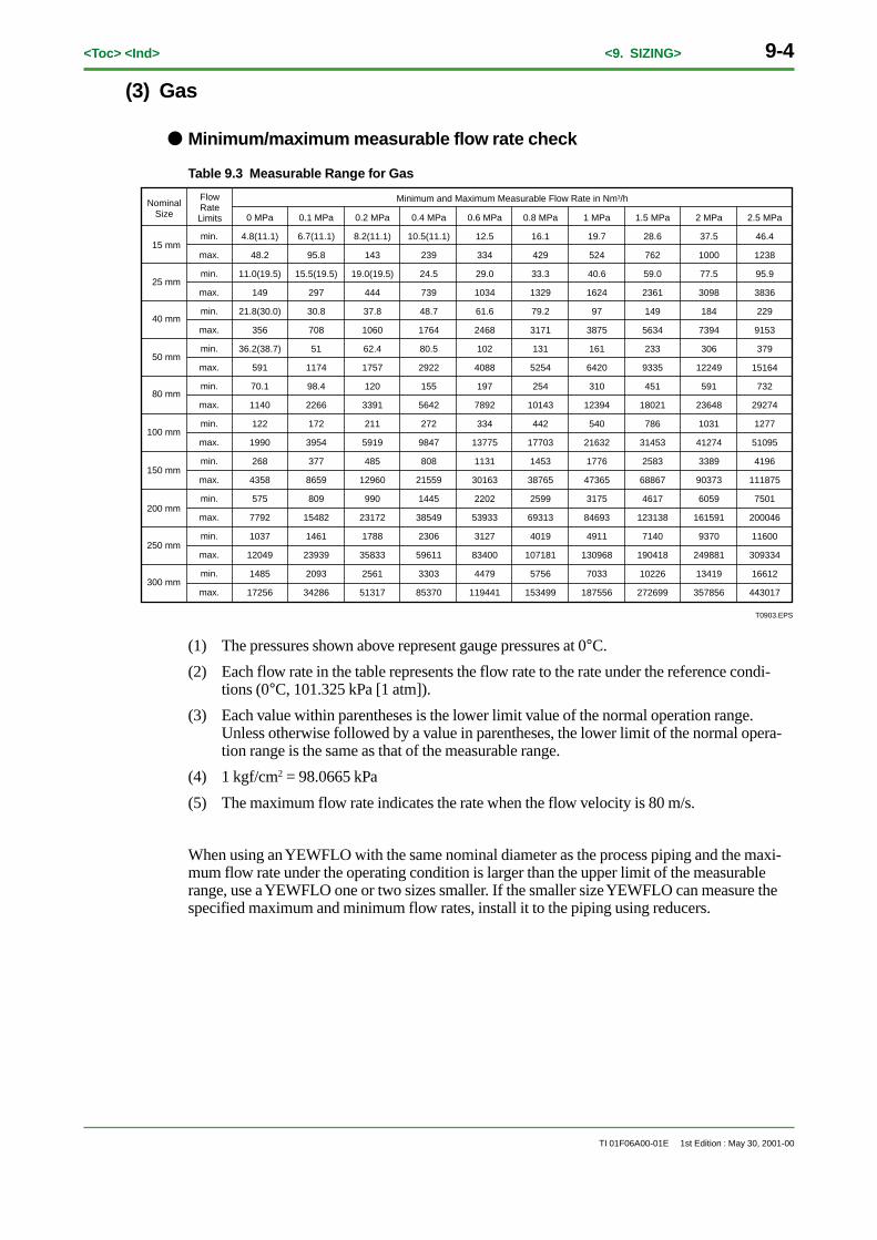
(3) Gas

● Minimum/maximum measurable flow rate check

Table 9.3 Measurable Range for Gas

min.

max.

min.

max.

min.

max.

min.

max.

min.

max.

min.

max.

min.

max.

min.

max.

min.

max.

min.

max.

15 mm

25 mm

40 mm

50 mm

80 mm

100 mm

150 mm

200 mm

250 mm

300 mm

NominalSize

FlowRateLimits

Minimum and Maximum Measurable Flow Rate in Nm3/h

0 MPa

4.8(11.1)

48.2

11.0(19.5)

149

21.8(30.0)

356

36.2(38.7)

591

70.1

1140

122

1990

268

4358

575

7792

1037

12049

1485

17256

0.1 MPa

6.7(11.1)

95.8

15.5(19.5)

297

30.8

708

51

1174

98.4

2266

172

3954

377

8659

809

15482

1461

23939

2093

34286

0.2 MPa

8.2(11.1)

143

19.0(19.5)

444

37.8

1060

62.4

1757

120

3391

211

5919

485

12960

990

23172

1788

35833

2561

51317

0.4 MPa

10.5(11.1)

239

24.5

739

48.7

1764

80.5

2922

155

5642

272

9847

808

21559

1445

38549

2306

59611

3303

85370

0.6 MPa

12.5

334

29.0

1034

61.6

2468

102

4088

197

7892

334

13775

1131

30163

2202

53933

3127

83400

4479

119441

0.8 MPa

16.1

429

33.3

1329

79.2

3171

131

5254

254

10143

442

17703

1453

38765

2599

69313

4019

107181

5756

153499

1 MPa

19.7

524

40.6

1624

97

3875

161

6420

310

12394

540

21632

1776

47365

3175

84693

4911

130968

7033

187556

1.5 MPa

28.6

762

59.0

2361

149

5634

233

9335

451

18021

786

31453

2583

68867

4617

123138

7140

190418

10226

272699

2 MPa

37.5

1000

77.5

3098

184

7394

306

12249

591

23648

1031

41274

3389

90373

6059

161591

9370

249881

13419

357856

2.5 MPa

46.4

1238

95.9

3836

229

9153

379

15164

732

29274

1277

51095

4196

111875

7501

200046

11600

309334

16612

443017

T0903.EPS

(1) The pressures shown above represent gauge pressures at 0°C.

(2) Each flow rate in the table represents the flow rate to the rate under the reference condi-tions (0°C, 101.325 kPa [1 atm]).

(3) Each value within parentheses is the lower limit value of the normal operation range.Unless otherwise followed by a value in parentheses, the lower limit of the normal opera-tion range is the same as that of the measurable range.

(4) 1 kgf/cm2 = 98.0665 kPa

(5) The maximum flow rate indicates the rate when the flow velocity is 80 m/s.

When using an YEWFLO with the same nominal diameter as the process piping and the maxi-mum flow rate under the operating condition is larger than the upper limit of the measurablerange, use a YEWFLO one or two sizes smaller. If the smaller size YEWFLO can measure thespecified maximum and minimum flow rates, install it to the piping using reducers.

../submenu.htm

../../index.htm



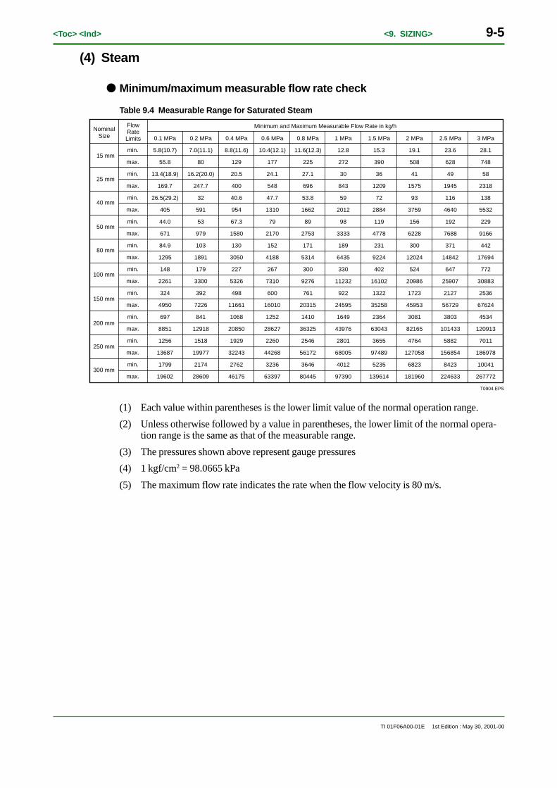
(4) Steam

● Minimum/maximum measurable flow rate check

Table 9.4 Measurable Range for Saturated Steam

min.

max.

min.

max.

min.

max.

min.

max.

min.

max.

min.

max.

min.

max.

min.

max.

min.

max.

min.

max.

15 mm

25 mm

40 mm

50 mm

80 mm

100 mm

150 mm

200 mm

250 mm

300 mm

NominalSize

FlowRateLimits

Minimum and Maximum Measurable Flow Rate in kg/h

0.1 MPa

5.8(10.7)

55.8

13.4(18.9)

169.7

26.5(29.2)

405

44.0

671

84.9

1295

148

2261

324

4950

697

8851

1256

13687

1799

19602

0.2 MPa

7.0(11.1)

80

16.2(20.0)

247.7

32

591

53

979

103

1891

179

3300

392

7226

841

12918

1518

19977

2174

28609

0.4 MPa

8.8(11.6)

129

20.5

400

40.6

954

67.3

1580

130

3050

227

5326

498

11661

1068

20850

1929

32243

2762

46175

0.6 MPa

10.4(12.1)

177

24.1

548

47.7

1310

79

2170

152

4188

267

7310

600

16010

1252

28627

2260

44268

3236

63397

0.8 MPa

11.6(12.3)

225

27.1

696

53.8

1662

89

2753

171

5314

300

9276

761

20315

1410

36325

2546

56172

3646

80445

1 MPa

12.8

272

30

843

59

2012

98

3333

189

6435

330

11232

922

24595

1649

43976

2801

68005

4012

97390

1.5 MPa

15.3

390

36

1209

72

2884

119

4778

231

9224

402

16102

1322

35258

2364

63043

3655

97489

5235

139614

2 MPa

19.1

508

41

1575

93

3759

156

6228

300

12024

524

20986

1723

45953

3081

82165

4764

127058

6823

181960

2.5 MPa

23.6

628

49

1945

116

4640

192

7688

371

14842

647

25907

2127

56729

3803

101433

5882

156854

8423

224633

3 MPa

28.1

748

58

2318

138

5532

229

9166

442

17694

772

30883

2536

67624

4534

120913

7011

186978

10041

267772

T0904.EPS

(1) Each value within parentheses is the lower limit value of the normal operation range.

(2) Unless otherwise followed by a value in parentheses, the lower limit of the normal opera-tion range is the same as that of the measurable range.

(3) The pressures shown above represent gauge pressures

(4) 1 kgf/cm2 = 98.0665 kPa

(5) The maximum flow rate indicates the rate when the flow velocity is 80 m/s.

../submenu.htm

../../index.htm



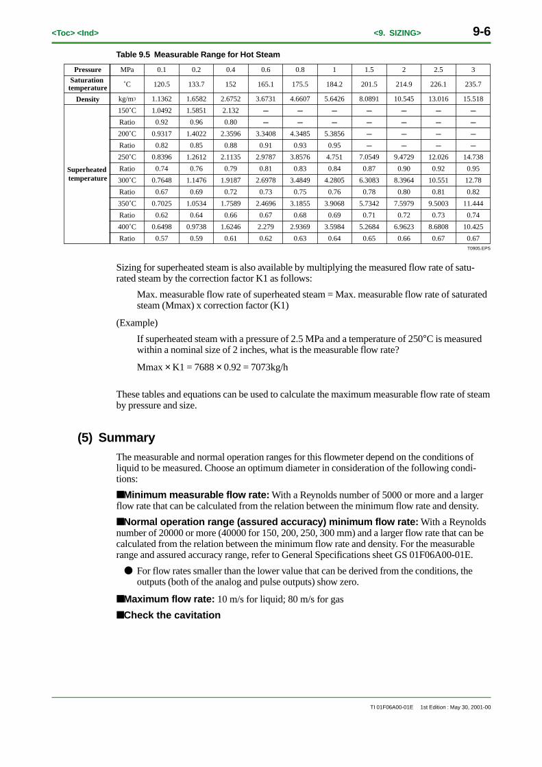
Table 9.5 Measurable Range for Hot Steam

Pressure Saturation

temperature Density

Superheated temperature

MPa

˚C

kg/m3

150˚C

Ratio

200˚C

Ratio

250˚C

Ratio

300˚C

Ratio

350˚C

Ratio

400˚C

Ratio

0.1

120.5

1.1362

1.0492

0.92

0.9317

0.82

0.8396

0.74

0.7648

0.67

0.7025

0.62

0.6498

0.57

0.2

133.7

1.6582

1.5851

0.96

1.4022

0.85

1.2612

0.76

1.1476

0.69

1.0534

0.64

0.9738

0.59

0.4

152

2.6752

2.132

0.80

2.3596

0.88

2.1135

0.79

1.9187

0.72

1.7589

0.66

1.6246

0.61

0.6

165.1

3.6731

---

---

3.3408

0.91

2.9787

0.81

2.6978

0.73

2.4696

0.67

2.279

0.62

0.8

175.5

4.6607

---

---

4.3485

0.93

3.8576

0.83

3.4849

0.75

3.1855

0.68

2.9369

0.63

1

184.2

5.6426

---

---

5.3856

0.95

4.751

0.84

4.2805

0.76

3.9068

0.69

3.5984

0.64

1.5

201.5

8.0891

---

---

---

---

7.0549

0.87

6.3083

0.78

5.7342

0.71

5.2684

0.65

2

214.9

10.545

---

---

---

---

9.4729

0.90

8.3964

0.80

7.5979

0.72

6.9623

0.66

2.5

226.1

13.016

---

---

---

---

12.026

0.92

10.551

0.81

9.5003

0.73

8.6808

0.67

3

235.7

15.518

---

---

---

---

14.738

0.95

12.78

0.82

11.444

0.74

10.425

0.67T0905.EPS

Sizing for superheated steam is also available by multiplying the measured flow rate of satu-rated steam by the correction factor K1 as follows:

Max. measurable flow rate of superheated steam = Max. measurable flow rate of saturatedsteam (Mmax) x correction factor (K1)

(Example)

If superheated steam with a pressure of 2.5 MPa and a temperature of 250°C is measuredwithin a nominal size of 2 inches, what is the measurable flow rate?

Mmax × K1 = 7688 × 0.92 = 7073kg/h

These tables and equations can be used to calculate the maximum measurable flow rate of steamby pressure and size.

(5) SummaryThe measurable and normal operation ranges for this flowmeter depend on the conditions ofliquid to be measured. Choose an optimum diameter in consideration of the following condi-tions:

■ Minimum measurable flow rate: With a Reynolds number of 5000 or more and a largerflow rate that can be calculated from the relation between the minimum flow rate and density.

■ Normal operation range (assured accuracy) minimum flow rate: With a Reynoldsnumber of 20000 or more (40000 for 150, 200, 250, 300 mm) and a larger flow rate that can becalculated from the relation between the minimum flow rate and density. For the measurablerange and assured accuracy range, refer to General Specifications sheet GS 01F06A00-01E.

● For flow rates smaller than the lower value that can be derived from the conditions, theoutputs (both of the analog and pulse outputs) show zero.

■ Maximum flow rate: 10 m/s for liquid; 80 m/s for gas

■ Check the cavitation

../submenu.htm

../../index.htm

<Toc> <Ind> <10. FLUID DATA> 10-1


10. FLUID DATA

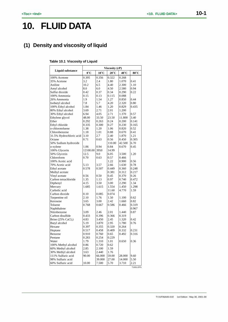
(1) Density and viscosity of liquid

Table 10.1 Viscosity of Liquid

Liquid substanceViscosity (cP)

0˚C

100% Acetone 35% Acetone AnilineAmyl alcoholSulfur dioxide100% Ammonia 26% Ammonia Isobutyl alcohol100% Ethyl alcohol 80% Ethyl alcohol 30% Ethyl alcohol Ethylene glycolEtherEthyl chlorideo-chlorotolueneChlorobenzene31.5% Hydrochloric acid Octane50% Sodium hydroxide o-xylene100% Glycerin50% Glycerin Chloroform 100% Acetic acid 70% Acetic acid Ethyl acetate Methyl acetateVinyl acetateCarbon tetrachlorideDiphenyl MercuryCarbolic acid Carbon dioxideTurpentine oil KeroseneTolueneNaphthaleneNitrobenzeneCarbon disulfideBrine (25% CaCl2)Butyl alcoholHexaneHeptaneBenzenePentaneWater100% Methyl alcohol 60% Methyl alcohol 30% Methyl alcohol 111% Sulfuric acid 98% Sulfuric acid 60% Sulfuric acid

0.3953.210.28.00.420.151.97.81.843.696.9448.000.2920.3351.381.183.100.71

1.0612100.0012.50.70

5.130.578

0.561.354.151.685

0.102.103.650.768

3.090.4334.835.190.3970.5170.9100.2831.790.862.853.6390.00

10.00

0.3562.46.56.00.370.131.545.71.462.714.0533.500.2630.3001.201.012.70.63

0.9439509.00.63

3.570.507

0.501.133.501.615

0.0851.763.000.667

2.460.3963.4503.8700.3550.4580.7600.2541.3100.7202.1002.44066.00039.0007.500

0.3221.804.404.500.340.1151.274.201.202.012.7123.500.240.271.060.882.400.56110.000.8414.996.050.571.222.660.4490.3810.450.973.001.55411.600.0741.502.420.586

2.010.3662.452.950.3200.4090.650.2291.010.621.591.7659.0027.005.70

0.2681.0702.3002.5800.2900.0880.8502.3200.8291.2001.37011.8000.2000.2300.8200.6701.8700.45042.5000.670

3.5000.4660.9001.6300.3600.3120.3700.7402.2901.4504.770

1.1001.6600.466

1.4400.3191.3201.7800.2640.3320.492

0.650

28.00014.0003.710

0.411.100.940.22

0.440.800.435

0.573.400.1410.1650.520.411.210.3056.700.45

1.20

0.560.780.2480.2170.260.4721.341.2981.59

0.620.820.3190.9670.87

0.420.76

0.2310.316

0.36

9.605.502.21

10˚C 20˚C 40˚C 80˚C

T1001.EPS

../submenu.htm

../../index.htm

10-2<Toc> <Ind> <10. FLUID DATA>


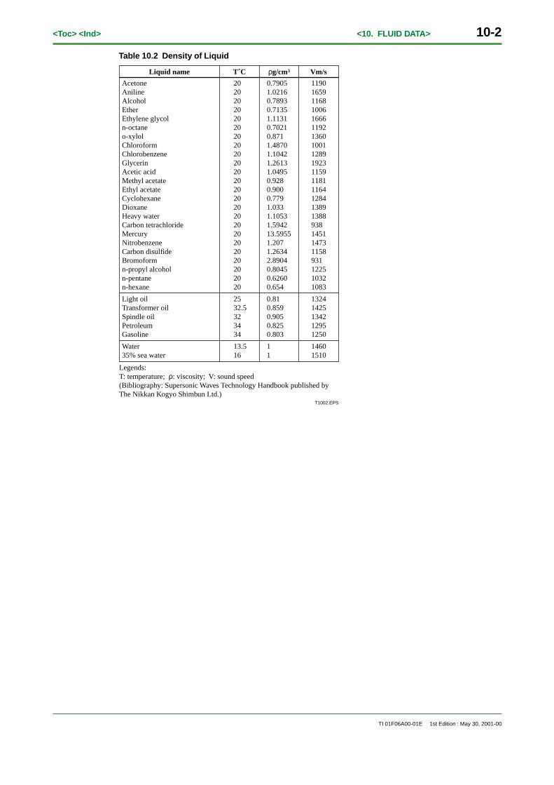
Table 10.2 Density of Liquid

Acetone AnilineAlcoholEtherEthylene glycoln-octaneo-xylolChloroform Chlorobenzene GlycerinAcetic acidMethyl acetate Ethyl acetateCyclohexaneDioxaneHeavy waterCarbon tetrachlorideMercuryNitrobenzeneCarbon disulfideBromoformn-propyl alcoholn-pentanen-hexane Light oilTransformer oilSpindle oilPetroleumGasoline Water35% sea water

202020202020202020202020202020202020202020202020 2532.5323434 13.516

0.79051.02160.78930.71351.11310.70210.8711.48701.10421.26131.04950.9280.9000.7791.0331.10531.594213.59551.2071.26342.89040.80450.62600.654 0.810.8590.9050.8250.803 11

1190165911681006166611921360100112891923115911811164128413891388938145114731158931122510321083 13241425134212951250 14601510

T˚CLiquid name ρg/cm3 Vm/s

T1002.EPS

Legends:T: temperature; ρ: viscosity; V: sound speed(Bibliography: Supersonic Waves Technology Handbook published by The Nikkan Kogyo Shimbun Ltd.)

../submenu.htm

../../index.htm

<Toc> <Ind> <10. FLUID DATA> 10-3


(2) Density and viscosity of gas

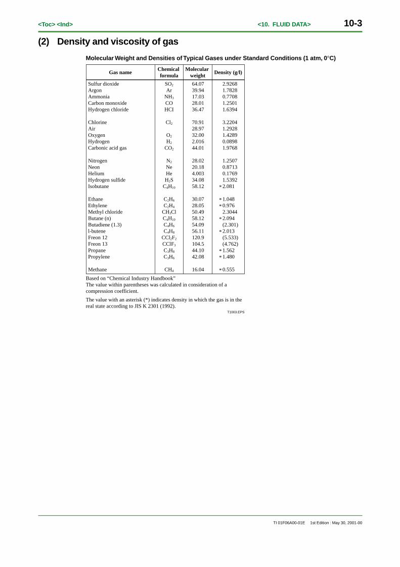
Molecular Weight and Densities of Typical Gases under Standard Conditions (1 atm, 0°C)

Sulfur dioxideArgonAmmoniaCarbon monoxideHydrogen chloride

ChlorineAirOxygenHydrogenCarbonic acid gas

NitrogenNeonHeliumHydrogen sulfideIsobutane

EthaneEthyleneMethyl chlorideButane (n)Butadiene (1.3)l-buteneFreon 12Freon 13PropanePropylene

Methane

SO2

ArNH3

COHCI

Cl2

O2

H2

CO2

N2

NeHeH2S

C4H10

C2H6

C2H4

CH3ClC4H10

C4H6

C4H8

CCl2F2

CClF3

C3H8

C3H6

CH4

64.0739.9417.0328.0136.47

70.9128.9732.002.01644.01

28.0220.184.00334.0858.12

30.0728.0550.4958.1254.0956.11120.9104.544.1042.08

16.04

2.92681.78280.77081.25011.6394

3.22041.29281.42890.08981.9768

1.25070.87130.17691.53922.081

1.0480.9762.30442.094(2.301)2.013(5.533)(4.762)1.5621.480

0.555

*

**

*

*

**

*

Chemical formula

Gas nameMolecular

weightDensity (g/l)

T1003.EPS

Based on “Chemical Industry Handbook”The value within parentheses was calculated in consideration of a compression coefficient. The value with an asterisk (*) indicates density in which the gas is in the real state according to JIS K 2301 (1992).

../submenu.htm

../../index.htm

10-4<Toc> <Ind> <10. FLUID DATA>


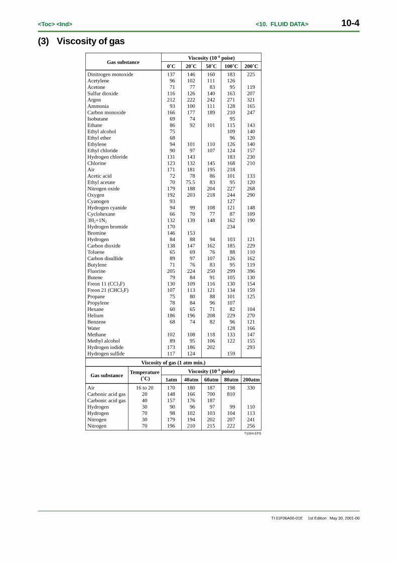
(3) Viscosity of gas

Gas substanceViscosity (10-6 poise)

0˚C

Dinitrogen monoxideAcetyleneAcetoneSulfur dioxideArgonAmmoniaCarbon monoxideIsobutaneEthaneEthyl alcoholEthyl etherEthyleneEthyl chlorideHydrogen chlorideChlorineAirAcetic acidEthyl acetateNitrogen oxideOxygenCyanogenHydrogen cyanideCyclohexane3H2+1N2

Hydrogen bromideBromineHydrogenCarbon dioxideTolueneCarbon disulfideButyleneFluorineButeneFreon 11 (CCl3F)Freon 21 (CHCl2F)PropanePropyleneHexaneHeliumBenzeneWaterMethaneMethyl alcoholHydrogen iodideHydrogen sulfide

1379671

116212

93166

698675689490

131123171

7270

179192

939466

132170146

84138

658971

20579

130107

757860

18668

10289

173117

146102

77126222100177

7492

10197

143132181

7875.5188203

9970

139

15388

147699776

22484

109113

808465

19674

10895

186124

160111

83140242111189

101

110107

145195

8683

204218

10877

148

94162

76107

83250

91116121

889671

20882

118106202

183126

95163271128210

95115109

96126124183168218101

95227244127121

87162234

103185

88126

95299105130134101107

82229

96128133122

159

225

119207321165247

143140120140157230210

133120268290

148109190

121229110162119396130154159125

104270121166147155293

20˚C 50˚C 100˚C 200˚C

Gas substance

Viscosity of gas (1 atm min.)

Viscosity (10-6 poise)Temperature (˚C) 1atm

AirCarbonic acid gasCarbonic acid gasHydrogenHydrogenNitrogenNitrogen

16 to 20204030703070

170148157

9098

179196

180166176

96102194210

187700187

97103202215

198810

99104207222

330

110113241256

40atm 60atm 80atm 200atm

T1004.EPS

../submenu.htm

../../index.htm

i<Int> <Toc> <Ind>

TI 01F06A00-01E

Revision Information● Title : Model DY Vortex Flowmeter

● Manual No. : TI 01F06A00-01E

May 2001/1st Edition/R1.02*Newly published

* : Denotes the release number of the software corresponding to the contents of this technical information.The revised contents are valid until the next edition is issued.

Written by Product Marketing Dept.Process Control Systems CenterIndustrial Automation Systems Business Div.Yokogawa Electric Corporation

Published by Yokogawa Electric Corporation2-9-32 Nakacho, Musashino-shi, Tokyo 180, JAPAN

Printed by Yokogawa Graphic Arts Co., Ltd.

1st Edition : May 30, 2001-00

../submenu.htm

../../index.htm

Blank Page

Documents

Technical Model DY Vortex Information Flowmeter