Embed Size (px)
Citation preview
Technical Support Document shyTechnical Update of the Social Cost of Carbon for Regulatory Impact Analysis shy
Under Executive Order 12866 shy
Interagency Working Group on Social Cost of Carbon United States Government
With participation by
Council of Economic Advisers Council on Environmental Quality
Department of Agriculture Department of Commerce
Department of Energy Department of Transportation
Environmental Protection Agency National Economic Council
Office of Management and Budget Office of Science and Technology Policy
Department of the Treasury
May 2013
Revised July 2015
See Appendix B for Details on Revision
1
Executive Summary
Under Executive Order 12866 agencies are θηϡΉθ φΩ φΆ ϲφφ εθΡΉφφ ϳ Λϭ φΩ μμμμ ΩφΆ
the costs and the benefits of the intended regulation and recognizing that some costs and benefits are
difficult to quantify propose or adopt a regulation only upon a reasoned determination that the
Ήφμ Ω φΆ Ήφ θͼϡΛφΉΩ ΕϡμφΉϳ Ήφμ Ωμφμ΄ ΐΆ εϡθεΩμ Ω φΆ μΩΉΛ Ωμφ Ω θΩ (ΊCC)
estimates presented here is to allow agencies to incorporate the social benefits of reducing carbon
dioxide (CO2) emissions into cost-benefit analyses of regulatory actions that impact cumulative global
emissions The SCC is an estimate of the monetized damages associated with an incremental increase in
carbon emissions in a given year It is intended to include (but is not limited to) changes in net
agricultural productivity human health property damages from increased flood risk and the value of
ecosystem services due to climate change
ΐΆ Ήφθͼϳ εθΩμμ φΆφ ϬΛΩε φΆ ΩθΉͼΉΛ Δ΄Ί΄ ͼΩϬθΡφμ ΊCC μφΉΡφμ Ήμ μθΉ Ή φΆ
2010 interagency technical support document (TSD) (Interagency Working Group on Social Cost of Carbon
2010) Through that process the interagency group selected four SCC values for use in regulatory analyses
Three values are based on the average SCC from three integrated assessment models (IAMs) at discount
rates of 25 3 and 5 percent The fourth value which represents the 95th percentile SCC estimate across
all three models at a 3 percent discount rate is included to represent higher-than-expected impacts from
temperature change further out in the tails of the SCC distribution
While acknowledging the continued limitations of the approach taken by the interagency group in 2010
this document provides an update of the SCC estimates based on new versions of each IAM (DICE PAGE
and FUND) It does not revisit other interagency modeling decisions (eg with regard to the discount rate
reference case socioeconomic and emission scenarios or equilibrium climate sensitivity) Improvements
in the way damages are modeled are confined to those that have been incorporated into the latest
versions of the models by the developers themselves in the peer-reviewed literature
The SCC estimates using the updated versions of the models are higher than those reported in the 2010
TSD By way of comparison the four 2020 SCC estimates reported in the 2010 TSD were $7 $26 $42 and
$81 (2007$) The corresponding four updated SCC estimates for 2020 are $12 $43 $64 and $128 (2007$)
The model updates that are relevant to the SCC estimates include an explicit representation of sea level
rise damages in the DICE and PAGE models updated adaptation assumptions revisions to ensure
damages are constrained by GDP updated regional scaling of damages and a revised treatment of
potentially abrupt shifts in climate damages in the PAGE model an updated carbon cycle in the DICE
model and updated damage functions for sea level rise impacts the agricultural sector and reduced
space heating requirements as well as changes to the transient response of temperature to the buildup
of GHG concentrations and the inclusion of indirect effects of methane emissions in the FUND model
The SCC estimates vary by year and the following table summarizes the revised SCC estimates from 2010
through 2050
2
Revised Social Cost of CO2 2010 ndash 2050 (in 2007 dollars per metric ton of CO2)
Discount Rate 50 30 25 30 Year Avg Avg Avg 95th 2010 10 31 50 86 2015 11 36 56 105 2020 12 42 62 123 2025 14 46 68 138 2030 16 50 73 152 2035 18 55 78 168 2040 21 60 84 183 2045 23 64 89 197 2050 26 69 95 212
3
I Purpose
The purpose of this document is to update the schedule of social cost of carbon (SCC) estimates from the
2010 interagency technical support document (TSD) (Interagency Working Group on Social Cost of Carbon
2010)1 E΄ͷ΄ 13563 ΩΡΡΉφμ φΆ ΡΉΉμφθφΉΩ φΩ θͼϡΛφΩθϳ ΉμΉΩ ΡΘΉͼ μ Ω φΆ μφ ϬΉΛΛ
science2 Additionally the interagency group recommended in 2010 that the SCC estimates be revisited
on a regular basis or as model updates that reflect the growing body of scientific and economic knowledge
become available3 New versions of the three integrated assessment models used by the US government
to estimate the SCC (DICE FUND and PAGE) are now available and have been published in the peer
reviewed literature While acknowledging the continued limitations of the approach taken by the
interagency group in 2010 (documented in the original 2010 TSD) this document provides an update of
the SCC estimates based on the latest peer-reviewed version of the models replacing model versions that
were developed up to ten years ago in a rapidly evolving field It does not revisit other assumptions with
regard to the discount rate reference case socioeconomic and emission scenarios or equilibrium climate
sensitivity Improvements in the way damages are modeled are confined to those that have been
incorporated into the latest versions of the models by the developers themselves in the peer-reviewed
literature The agencies participating in the interagency working group continue to investigate potential
improvements to the way in which economic damages associated with changes in CO2 emissions are
quantified
Section II summarizes the major updates relevant to SCC estimation that are contained in the new versions
of the integrated assessment models released since the 2010 interagency report Section III presents the
updated schedule of SCC estimates for 2010 ndash 2050 based on these versions of the models Section IV
provides a discussion of other model limitations and research gaps
II Summary of Model Updates
This section briefly summarizes changes to the most recent versions of the three integrated assessment
models (IAMs) used by the interagency group in 2010 We focus on describing those model updates that
are relevant to estimating the social cost of carbon as summarized in Table 1 For example both the DICE
and PAGE models now include an explicit representation of sea level rise damages Other revisions to
PAGE include updated adaptation assumptions revisions to ensure damages are constrained by GDP
updated regional scaling of damages and a revised treatment of potentially abrupt shifts in climate
damages The DICE ΡΩΛμ μΉΡεΛ θΩ ϳΛ Άμ ϡεφ φΩ more consistent with a more
complex climate model The FUND model includes updated damage functions for sea level rise impacts
the agricultural sector and reduced space heating requirements as well as changes to the transient
response of temperature to the buildup of GHG concentrations and the inclusion of indirect effects of
1 In this document we present all values of the SCC as the cost per metric ton of CO2 emissions Alternatively one could report the SCC as the cost per metric ton of carbon emissions The multiplier for translating between mass of CO2 and the mass of carbon is 367 (the molecular weight of CO2 divided by the molecular weight of carbon = 4412 = 367) 2 httpwwwwhitehousegovsitesdefaultfilesombinforegeo12866eo13563_01182011pdf 3 See p 1 3 4 29 and 33 (Interagency Working Group on Social Cost of Carbon 2010)
4
methane emissions Changes made to parts of the models that are superseded by the interagency working
ͼθΩϡεμ ΡΩΛΉͼ μμϡΡεφΉΩs ndash regarding equilibrium climate sensitivity discounting and
socioeconomic variables ndash are not discussed here but can be found in the references provided in each
section below
Table 1 Summary of Key Model Revisions Relevant to the Interagency SCC
IAM Version used in 2010 Interagency
Analysis
New Version
Key changes relevant to interagency SCC
DICE 2007 2010 Updated calibration of the carbon cycle model and explicit representation of sea level rise (SLR) and associated damages
FUND 35 (2009)
38 (2012)
Updated damage functions for space heating SLR agricultural impacts changes to transient response of temperature to buildup of GHG concentrations and inclusion of indirect climate effects of methane
PAGE 2002 2009 Explicit representation of SLR damages revisions to damage function to ensure damages do not exceed 100 of GDP change in regional scaling of damages revised treatment of potential abrupt damages and updated adaptation assumptions
A DICE
DICE 2010 includes a number of changes over the previous 2007 version used in the 2010 interagency
report The model changes that are relevant for the SCC estimates developed by the interagency working
group include 1) updated parameter values for the carbon cycle model 2) an explicit representation of
sea level dynamics and 3) a re-calibrated damage function that includes an explicit representation of
economic damages from sea level rise Changes were also made to other parts of the DICE modelmdash
including the equilibrium climate sensitivity parameter the rate of change of total factor productivity and
the elasticity of the marginal utility of consumptionmdashbut these components of DICE are superseded by
the interagency working groupμ assumptions and so will not be discussed here More details on DICE2007
can be found in Nordhaus (2008) and on DICE2010 in Nordhaus (2010) The DICE2010 model and
documentation is also available for download from the homepage of William Nordhaus
Carbon Cycle Parameters
DICE uses a three-box model of carbon stocks and flows to represent the accumulation and transfer of
carbon among the atmosphere the shallow ocean and terrestrial biosphere and the deep ocean These
εθΡφθμ θ ΛΉθφ φΩ ΡφΆ φΆ θΩ ϳΛ Ή φΆ Ͱodel for the Assessment of Greenhouse
Gμ ϡ CΛΉΡφ CΆͼ (ͰGCC) (ͱΩθΆϡμ 2008 ε 44)4 Carbon cycle transfer coefficient values
4 MAGICC is a simple climate model initially developed by the US National Center for Atmospheric Research that has been used heavily by the Intergovernmental Panel on Climate Change (IPCC) to emulate projections from more sophisticated state of the art earth system simulation models (Randall et al 2007)
5
in DICE2010 are based on re-calibration of the model to match the newer 2009 version of MAGICC
(Nordhaus 2010 p 2) For example in DICE2010 in each decade 12 percent of the carbon in the
atmosphere is transferred to the shallow ocean 47 percent of the carbon in the shallow ocean is
transferred to the atmosphere 948 percent remains in the shallow ocean and 05 percent is transferred
to the deep ocean For comparison in DICE 2007 189 percent of the carbon in the atmosphere is
transferred to the shallow ocean each decade 97 percent of the carbon in the shallow ocean is
transferred to the atmosphere 853 percent remains in the shallow ocean and 5 percent is transferred
to the deep ocean
The implication of these changes for DICE2010 is in general a weakening of the ocean as a carbon sink and
therefore a higher concentration of carbon in the atmosphere than in DICE2007 for a given path of
emissions All else equal these changes will generally increase the level of warming and therefore the SCC
estimates in DICE2010 relative to those from DICE2007
Sea Level Dynamics
A new feature of DICE2010 is an explicit representation of the dynamics of the global average sea level
anomaly to be used in the updated damage function (discussed below) This section contains a brief
description of the sea level rise (SLR) module a more detailed description can be found on the model
ϬΛΩεθμ ϭμΉφ΄5 The average global sea level anomaly is modeled as the sum of four terms that
represent contributions from 1) thermal expansion of the oceans 2) melting of glaciers and small ice
caps 3) melting of the Greenland ice sheet and 4) melting of the Antarctic ice sheet
The parameters of the four components of the SLR module are calibrated to match consensus results from
φΆ CCμ FΩϡθφΆ μμμμΡφ ΆεΩθφ (AR4)6 The rise in sea level from thermal expansion in each time
period (decade) is 2 percent of the difference between the sea level in the previous period and the long
run equilibrium sea level which is 05 meters per degree Celsius (degC) above the average global
temperature in 1900 The rise in sea level from the melting of glaciers and small ice caps occurs at a rate
of 0008 meters per decade per degC above the average global temperature in 1900
The contribution to sea level rise from melting of the Greenland ice sheet is more complex The
equilibrium contribution to SLR is 0 meters for temperature anomalies less than 1 oC and increases linearly
from 0 meters to a maximum of 73 meters for temperature anomalies between 1 oC and 35 degC The
contribution to SLR in each period is proportional to the difference between the previΩϡμ εθΉΩμ μ
level anomaly and the equilibrium sea level anomaly where the constant of proportionality increases with
the temperature anomaly in the current period
5 Documentation on the new sea level rise module of DICE is available on William NordΆϡμ ϭμΉφ φ httpnordhauseconyaleedudocumentsSLR_021910pdf 6 For a review of post-IPCC AR4 research on sea level rise see Nicholls et al (2011) and NAS (2011)
6
The contribution to SLR from the melting of the Antarctic ice sheet is -0001 meters per decade when the
temperature anomaly is below 3 degC and increases linearly between 3 degC and 6 degC to a maximum rate of
0025 meters per decade at a temperature anomaly of 6 degC
Re-calibrated Damage Function
Economic damages from climate change in the DICE model are represented by a fractional loss of gross
economic output in each period A portion of the remaining economic output in each period (net of
climate change damages) is consumed and the remainder is invested in the physical capital stock to
support future economic εθΩϡφΉΩ μΩ Ά εθΉΩμ ΛΉΡφ Ρͼμ ϭΉΛΛ θϡ ΩμϡΡεφΉΩ Ή φΆφ
period and in all future periods due to the lost investment The fraction of output in each period that is
lost due to climate change impacts is represented as one minus a fraction which is one divided by a
ηϡθφΉ ϡφΉΩ Ω φΆ φΡεθφϡθ ΩΡΛϳ εθΩϡΉͼ μΉͼΡΩΉ (Ί-shaped) function7 The loss
function in DICE2010 has been expanded by adding a quadratic function of SLR to the quadratic function
of temperature In DICE2010 the temperature anomaly coefficients have been recalibrated to avoid
double-counting damages from sea level rise that were implicitly included in these parameters in
DICE2007
ΐΆ ͼͼθͼφ Ρͼμ Ή DCE2010 θ ΉΛΛϡμφθφ ϳ ͱΩθΆϡμ (2010 ε 3) ϭΆΩ Ωφμ φΆφ ΅Ρͼμ
in the uncontrolled (baseline) [ie reference] case ΅ Ή 2095 θ $12 φθΉΛΛΉΩ Ωθ 2΄8 εθφ Ω ͼΛΩΛ
output for a global temperature increase of 34 oC ΩϬ 1900 ΛϬΛμ΄ ΐΆΉμ ΩΡεθμ φΩ ΛΩμμ Ω 3΄2
percent of global output at 34 oC in DICE2007 However in DICE2010 annual damages are lower in most
of the early periods of the modeling horizon but higher in later periods than would be calculated using
the DICE2007 damage function Specifically the percent difference between damages in the base run of
DICE2010 and those that would be calculated using the DICE2007 damage function starts at +7 percent in
2005 decreases to a low of -14 percent in 2065 then continuously increases to +20 percent by 2300 (the
end of the interagency analysis time horizon) and to +160 percent by the end of the model time horizon
in 2595 The large increases in the far future years of the time horizon are due to the permanence
associated with damages from sea level rise along with the assumption that the sea level is projected to
continue to rise long after the global average temperature begins to decrease The changes to the loss
function generally decrease the interagency working group SCC estimates slightly given that relative
increases in damages in later periods are discounted more heavily all else equal
B FUND
FUND version 38 includes a number of changes over the previous version 35 (Narita et al 2010) used in
the 2010 interagency report Documentation supporting FUND φΆ ΡΩΛμ μΩϡθ Ω for all
versions of the model is available from the model authors8 Notable changes due to their impact on the
7 The model and documentation including formulas are available on the authorμ webpage at httpwwweconyaleedu~nordhaushomepageRICEmodelshtm 8 httpwwwfund-modelorg This report uses version 38 of the FUND model which represents a modest update to the most recent version of the model to appear in the literature (version 37) (Anthoff and Tol 2013) For the purpose of computing the SCC the relevant changes (between 37 to 38) are associated with improving
7
SCC estimates are adjustments to the space heating agriculture and sea level rise damage functions in
addition to changes to the temperature response function and the inclusion of indirect effects from
methane emissions9 We discuss each of these in turn
Space Heating
In FUND the damages associated with the change in energy needs for space heating are based on the
estimated impact due to one degree of warming These baseline damages are scaled based on the
Ωθμφ φΡεθφϡθ ΩΡΛϳμ ϬΉφΉΩ θΩΡ φΆ Ω ͼθ ΆΡθΘ and adjusted for changes
in vulnerability due to economic and energy efficiency growth In FUND 35 the function that scales the
base year damages adjusted for vulnerability allows for the possibility that in some simulations the
benefits associated with reduced heating needs may be an unbounded convex function of the
temperature anomaly In FUND 38 the form of the scaling has been modified to ensure that the function
is everywhere concave and that there will exist an upper bound on the benefits a region may receive from
reduced space heating needs The new formulation approaches a value of two in the limit of large
temperature anomalies or in other words assuming no decrease in vulnerability the reduced
expenditures on space heating at any level of warming will not exceed two times the reductions
experienced at one degree of warming Since the reduced need for space heating represents a benefit of
climate change in the model or a negative damage this change will increase the estimated SCC This
update accounts for a significant portion of the difference in the expected SCC estimates reported by the
two versions of the model when run probabilistically
Sea Level Rise and Land Loss
The FUND model explicitly includes damages associated with the inundation of dry land due to sea level
rise The amount of land lost within a region is dependent upon the proportion of the coastline being
protected by adequate sea walls and the amount of sea level rise In FUND 35 the function defining the
potential land lost in a given year due to sea level rise is linear in the rate of sea level rise for that year
This assumption implicitly assumes that all regions are well represented by a homogeneous coastline in
length and a constant uniform slope moving inland In FUND 38 the function defining the potential land
lost has been changed to be a convex function of sea level rise thereby assuming that the slope of the
shore line increases moving inland The effect of this change is to typically reduce the vulnerability of
some regions to sea level rise based land loss thereby lowering the expected SCC estimate 10
consistency with IPCC AR4 by adjusting the atmospheric lifetimes of CH4 and N2O and incorporating the indirect forcing effects of CH4 along with making minor stability improvements in the sea wall construction algorithm 9 The other damage sectors (water resources space cooling land loss migration ecosystems human health and extreme weather) were not significantly updated 10 For stability purposes this report also uses an update to the model which assumes that regional coastal protection measures will be built to protect the most valuable land first such that the marginal benefits of coastal protection is decreasing in the level of protection following Fankhauser (1995)
8
Agriculture
In FUND φΆ Ρͼμ μμΩΉφ ϭΉφΆ φΆ ͼθΉϡΛφϡθΛ μφΩθ θ Ρμϡθ μ εθΩεΩθφΉΩΛ φΩ φΆ μφΩθμ
value The fraction is bounded from above by one and is made up of three additive components that
represent the effects from carbon fertilization the rate of temperature change and the level of the
temperature anomaly In both FUND 35 and FUND 38 the θφΉΩ Ω φΆ μφΩθμ ϬΛϡ ΛΩμφ ϡ φΩ φΆ
level of the temperature anomaly is modeled as a quadratic function with an intercept of zero In FUND
35 the coefficients of this loss function are modeled as the ratio of two random normal variables This
specification had the potential for unintended extreme behavior as draws from the parameter in the
denominator approached zero or went negative In FUND 38 the coefficients are drawn directly from
truncated normal distributions so that they remain in the range [0 ) and ( 0] respectively ensuring
the correct sign and eliminating the potential for divide by zero errors The means for the new
distributions are set equal to the ratio of the means from the normal distributions used in the previous
version In general the impact of this change has been to decrease the range of the distribution while
spreading out the dΉμφθΉϡφΉΩμ Ρμμ ΩϬθ φΆ θΡΉΉͼ θͼ relative to the previous version The net
effect of this change on the SCC estimates is difficult to predict
Transient Temperature Response
The temperature response model translates changes in global levels of radiative forcing into the current
expected temperature anomaly In FUND a given years increase in the temperature anomaly is based on
a mean reverting function where the mean equals the equilibrium temperature anomaly that would
eventually be reached i φΆφ ϳθμ ΛϬΛ Ω θΉφΉϬ ΩθΉͼ were sustained The rate of mean reversion
defines the rate at which the transient temperature approaches the equilibrium In FUND 35 the rate of
temperature response is defined as a decreasing linear function of equilibrium climate sensitivity to
capture the fact that the progressive heat uptake of the deep ocean causes the rate to slow at higher
values of the equilibrium climate sensitivity In FUND 38 the rate of temperature response has been
updated to a quadratic function of the equilibrium climate sensitivity This change reduces the sensitivity
of the rate of temperature response to the level of the equilibrium climate sensitivity a relationship first
noted by Hansen et al (1985) based on the heat uptake of the deep ocean Therefore in FUND 38 the
temperature response will typically be faster than in the previous version The overall effect of this change
is likely to increase estimates of the SCC as higher temperatures are reached during the timeframe
analyzed and as the same damages experienced in the previous version of the model are now experienced
earlier and therefore discounted less
Methane
The IPCC AR4 notes a series of indirect effects of methane emissions and has developed methods for
proxying such effects when computing the global warming potential of methane (Forster et al 2007)
FUND 38 now includes the same methods for incorporating the indirect effects of methane emissions
Specifically the average atmospheric lifetime of methane has been set to 12 years to account for the
feedback of methane emissions on its own lifetime The radiative forcing associated with atmospheric
methane has also been increased by 40 to account for its net impact on ozone production and
9
stratospheric water vapor All else equal the effect of this increased radiative forcing will be to increase
the estimated SCC values due to greater projected temperature anomaly
C PAGE
PAGE09 (Hope 2013) includes a number of changes from PAGE2002 the version used in the 2010 SCC
interagency report The changes that most directly affect the SCC estimates include explicitly modeling
the impacts from sea level rise revisions to the damage function to ensure damages are constrained by
GDP a change in the regional scaling of damages a revised treatment for the probability of a discontinuity
within the damage function and revised assumptions on adaptation The model also includes revisions to
the carbon cycle feedback and the calculation of regional temperatures11 More details on PAGE09 can be
found in Hope (2011a 2011b 2011c) A description of PAGE2002 can be found in Hope (2006)
Sea Level Rise
While PAGE2002 aggregates all damages into two categories ndash economic and non-economic impacts -
PAGE09 adds a third explicit category damages from sea level rise In the previous version of the model
damages from sea level rise were subsumed by the other damage categories In PAGE09 sea level damages
increase less than linearly with sea level under the assumption that land people and GDP are more
concentrated in low-lying shoreline areas Damages from the economic and non-economic sector were
adjusted to account for the introduction of this new category
Revised Damage Function to Account for Saturation
In PAGE09 small initial economic and non-economic benefits (negative damages) are modeled for small
temperature increases but all regions eventually experience economic damages from climate change
where damages are the sum of additively separable polynomial functions of temperature and sea level
rise Damages transition from this polynomial function to a logistic path once they exceed a certain
proportion of remaining Gross Domestic Product (GDP) to ensure that damages do not exceed 100 percent
of GDP This differs from PAGE2002 which allowed Eastern Europe to potentially experience large
benefits from temperature increases and which also did not bound the possible damages that could be
experienced
Regional Scaling Factors
As in the previous version of PAGE the PAGE09 model calculates the damages for the European Union
(EU) and then assumes that damages for other regions are proportional based on a given scaling factor
The scaling factor in PAGE09 is based on the ΛͼφΆ Ω θͼΉΩμ ΩμφΛΉ θΛφΉϬ φΩ φΆ EΔ (Hope 2011b)
Because of the long coastline in the EU other regions are on average less vulnerable than the EU for the
same sea level and temperature increase but all regions have a positive scaling factor PAGE2002 based
Ήφμ μΛΉͼ φΩθμ Ω Ωϡθ μφϡΉμ θεΩθφ Ή φΆ CCμ φΆΉθ μμμμΡφ report and allowed for benefits
11 Because several changes in the PAGE model are structural (eg the addition of sea level rise and treatment of discontinuity) it is not possible to assess the direct impact of each change on the SCC in isolation as done for the other two models above
10
from temperature increase in Eastern Europe smaller impacts in developed countries and higher
damages in developing countries
Probability of a Discontinuity
GE2002 φΆ Ρͼμ μμΩΉφ ϭΉφΆ ΉμΩφΉϡΉφϳ (nonlinear extreme event) were modeled
as an expected value Specifically a stochastic probability of a discontinuity was multiplied by the
damages associated with a discontinuity to obtain an expected value and this was added to the
economic and non-economic impacts That is additional damages from an extreme event such as
extreme melting of the Greenland ice sheet were multiplied by the probability of the event occurring
and added to the damage estimate In PAGE09 the probability of discontinuity is treated as a discrete
event for each year in the model The damages for each model run are estimated either with or without
a discontinuity occurring rather than as an expected value A large‐scale discontinuity becomes possible
when the temperature rises beyond some threshold value between 2 and 4degC The probability that a
discontinuity will occur beyond this threshold then increases by between 10 and 30 percent for every
1degC rise in temperature beyond the threshold If a discontinuity occurs the EU loses an additional 5 to
25 percent of its GDP (drawn from a triangular distribution with a mean of 15 percent) in addition to
other damages and other regions lose an amount determined by the regional scaling factor The
threshold value for a possible discontinuity is lower than in PAGE2002 while the rate at which the
probability of a discontinuity increases with the temperature anomaly and the damages that result from
a discontinuity are both higher than in PAGE2002 The model assumes that only one discontinuity can
occur and that the impact is phased in over a period of time but once it occurs its effect is permanent
Adaptation
As in PAGE2002 adaptation is available to help mitigate any climate change impacts that occur In PAGE
this adaptation is the same regardless of the temperature change or sea level rise and is therefore akin to
what is more commonly considered a reduction in vulnerability It is modeled by reducing the damages
by some percentage PAGE09 assumes a smaller decrease in vulnerability than the previous version of the
model and assumes that it will take longer for this change in vulnerability to be realized In the aggregated
economic sector at the time of full implementation this adaptation will mitigate all damages up to a
temperature increase of 1degC and for temperature anomalies between 1degC and 2degC it will reduce damages
by 15-30 percent (depending on the region) However it takes 20 years to fully implement this adaptation
In PAGE2002 adaptation was assumed to reduce economic sector damages up to 2degC by 50-90 percent
after 20 years Beyond 2degC no adaptation is assumed to be available to mitigate the impacts of climate
change For the non-economic sector in PAGE09 adaptation is available to reduce 15 percent of the
damages due to a temperature increase between 0degC and 2degC and is assumed to take 40 years to fully
implement instead of 25 percent of the damages over 20 years assumed in PAGE2002 Similarly
adaptation is assumed to alleviate 25-50 percent of the damages from the first 020 to 025 meters of sea
level rise but is assumed to be ineffective thereafter Hope (2011c) estimates that the less optimistic
assumptions regarding the ability to offset impacts of temperature and sea level rise via adaptation
increase the SCC by approximately 30 percent
11
Other Noteworthy Changes
Two other changes in the model are worth noting There is a change in the way the model accounts for
decreased CO2 absorption on land and in the ocean as temperature rises PAGE09 introduces a linear
feedback from global mean temperature to the percentage gain in the excess concentration of CO2
capped at a maximum level In PAGE2002 an additional amount was added to the CO2 emissions each
period to account for a decrease in ocean absorption and a loss of soil carbon Also updated is the method
by which the average global and annual temperature anomaly is downscaled to determine annual average
regional temperature anomalies to be used in the regional damage functions In PAGE2002 the scaling
was determined solely based on regional difference in emissions of sulfate aerosols In PAGE09 this
regional temperature anomaly is further adjusted using an additive factor that is based on the average
absolute latitude of a region relative to the area weighted average absolute laφΉφϡ Ω φΆ EθφΆμ
landmass to capture relatively greater changes in temperature forecast to be experienced at higher
latitudes
III Revised SCC Estimates
The updated versions of the three integrated assessment models were run using the same methodology
detailed in the 2010 TSD (Interagency Working Group on Social Cost of Carbon 2010) The approach along
with the inputs for the socioeconomic emissions scenarios equilibrium climate sensitivity distribution
and discount rate remains the same This includes the five reference scenarios based on the EMF-22
modeling exercise the Roe and Baker equilibrium climate sensitivity distribution calibrated to the IPCC
AR4 and three constant discount rates of 25 3 and 5 percent
As was previously the case the use of three models three discount rates and five scenarios produces 45
separate distributions for the global SCC The approach laid out in the 2010 TSD applied equal weight to
each model and socioeconomic scenario in order to reduce the dimensionality down to three separate
distributions representative of the three discount rates The interagency group selected four values from
these distributions for use in regulatory analysis Three values are based on the average SCC across models
and socio-economic-emissions scenarios at the 25 3 and 5 percent discount rates respectively The
fourth value was chosen to represent the higher-than-expected economic impacts from climate change
further out in the tails of the SCC distribution For this purpose the 95th percentile of the SCC estimates
at a 3 percent discount rate was chosen (A detailed set of percentiles by model and scenario combination
and additional summary statistics for the 2020 values is available in the Appendix) As noted in the 2010
TSD the 3 percent discount rate is the central value and so the central value that emerges is the average
SCC across models at the 3 percent discount rate (Interagency Working Group on Social Cost of Carbon
2010 p 25) However for purposes of capturing the uncertainties involved in regulatory impact analysis
the interagency group emphasizes the importance and value of including all four SCC values
Table 2 shows the four selected SCC estimates in five year increments from 2010 to 2050 Values for 2010
2020 2030 2040 and 2050 are calculated by first combining all outputs (10000 estimates per model run)
from all scenarios and models for a given discount rate Values for the years in between are calculated
12
using linear interpolation The full set of revised annual SCC estimates between 2010 and 2050 is reported
in the Appendix
Table 2 Revised Social Cost of CO2 2010 ndash 2050 (in 2007 dollars per metric ton of CO2)
Discount Rate 50 30 25 30 Year Avg Avg Avg 95th 2010 10 31 50 86 2015 11 36 56 105 2020 12 42 62 123 2025 14 46 68 138 2030 16 50 73 152 2035 18 55 78 168 2040 21 60 84 183 2045 23 64 89 197 2050 26 69 95 212
The SCC estimates using the updated versions of the models are higher than those reported in the 2010
TSD due to the changes to the models outlined in the previous section By way of comparison the 2020
SCC estimates reported in the original TSD were $7 $26 $42 and $81 (2007$) (Interagency Working Group
on Social Cost of Carbon 2010) Figure 1 illustrates where the four SCC values for 2020 fall within the full
distribution for each discount rate based on the combined set of runs for each model and scenario
(150000 estimates in total for each discount rate) In general the distributions are skewed to the right
and have long tails The Figure also shows that the lower the discount rate the longer the right tail of the
distribution
Figure 1 Distribution of SCC Estimates for 2020 (in 2007$ per metric ton CO2)
As was the case in the 2010 TSD the SCC increases over time because future emissions are expected to
produce larger incremental damages as physical and economic systems become more stressed in
13
response to greater climatic change The approach taken by the interagency group is to compute the cost
of a marginal ton emitted in the future by running the models for a set of perturbation years out to 2050
Table 3 illustrates how the growth rate for these four SCC estimates varies over time
Table 3 Average Annual Growth Rates of SCC Estimates between 2010 and 2050
Average Annual Growth Rate ()
50 Avg
30 Avg
25 Avg
30 95th
2010-2020 2020-2030 2030-2040 2040-2050
12 34 30 26
32 21 19 16
24 17 15 13
44 23 20 16
The future monetized value of emission reductions in each year (the SCC in year t multiplied by the change
in emissions in year t) must be discounted to the present to determine its total net present value for use
in regulatory analysis As previously discussed in the 2010 TSD damages from future emissions should be
discounted at the same rate as that used to calculate the SCC estimates themselves to ensure internal
consistency ndash ie future damages from climate change whether they result from emissions today or
emissions in a later year should be discounted using the same rate
Under current OMB guidance contained in Circular A-4 analysis of economically significant proposed
and final regulations from the domestic perspective is required while analysis from the international
perspective is optional However the climate change problem is highly unusual in at least two respects
First it involves a global externality emissions of most greenhouse gases contribute to damages around
the world even when they are emitted in the United States Consequently to address the global nature
of the problem the SCC must incorporate the full (global) damages caused by GHG emissions Second
climate change presents a problem that the United States alone cannot solve Even if the United States
were to reduce its greenhouse gas emissions to zero that step would be far from enough to avoid
substantial climate change Other countries would also need to take action to reduce emissions if
significant changes in the global climate are to be avoided Emphasizing the need for a global solution to
a global problem the United States has been actively involved in seeking international agreements to
reduce emissions and in encouraging other nations including emerging major economies to take
significant steps to reduce emissions When these considerations are taken as a whole the interagency
group concluded that a global measure of the benefits from reducing US emissions is preferable For
additional discussion see the 2010 TSD
IV Other Model Limitations and Research Gaps
The 2010 interagency SCC TSD discusses a number of important limitations for which additional research
is needed In particular the document highlights the need to improve the quantification of both non-
catastrophic and catastrophic damages the treatment of adaptation and technological change and the
way in which inter-regional and inter-sectoral linkages are modeled While the new version of the models
discussed above offer some improvements in these areas further work remains warranted The 2010 TSD
also discusses the need to more carefully assess the implications of risk aversion for SCC estimation as
14
well as the inability to perfectly substitute between climate and non-climate goods at higher temperature
increases both of which have implications for the discount rate used EPA DOE and other agencies
continue to engage in research on modeling and valuation of climate impacts that can potentially improve
SCC estimation in the future
References
Anthoff D and Tol RSJ 2013 The uncertainty about the social cost of carbon a decomposition analysis using FUND Climatic Change 117 515ndash530
Anthoff D and Tol RSJ 2013 Erratum to The uncertainty about the social cost of carbon A decomposition analysis using FUND Climatic Change Advance online publication doi 101007s10584shy013-0959-1
Fankhauser S 1995 Valuing climate change The economics of the greenhouse London England Earthscan
Forster P V Ramaswamy P Artaxo T Berntsen R Betts DW Fahey J Haywood J Lean DC Lowe
G Myhre J Nganga R Prinn G Raga M Schulz and R Van Dorland 2007 Changes in Atmospheric
Constituents and in Radiative Forcing In Climate Change 2007 The Physical Science Basis Contribution
of Working Group I to the Fourth Assessment Report of the Intergovernmental Panel on Climate Change
[Solomon S D Qin M Manning Z Chen M Marquis KB Averyt MTignor and HL Miller (eds)]
Cambridge University Press Cambridge United Kingdom and New York NY USA
HΩε CΆθΉμ΄ 2006΄ ΐΆ ͰθͼΉΛ Ρεφ Ω Cͷ2 from PAGE2002 An Integrated Assessment Model
ΩθεΩθφΉͼ φΆ CCμ FΉϬ ΆμΩμ Ωθ CΩθ΄ The Integrated Assessment Journal 6(1) 19ndash56
HΩε CΆθΉμ΄ 2011 The PAGE09 Integrated Assessment Model A Technical Description Cambridge
Judge Business School Working Paper No 42011 (April) Accessed November 23 2011
httpwwwjbscamacukresearchworking_papers2011wp1104pdf
HΩε CΆθΉμ΄ 2011 The Social Cost of CO2 from the PAGE09 Model Cambridge Judge Business School
Working Paper No 52011 (June) Accessed November 23 2011
httpwwwjbscamacukresearchworking_papers2011wp1105pdf
HΩε CΆθΉμ΄ 2011 New Insights from the PAGE09 Model The Social Cost of CO2 Cambridge Judge
Business School Working Paper No 82011 (July) Accessed November 23 2011
httpwwwjbscamacukresearchworking_papers2011wp1108pdf
Hope C 2013 Critical issues for the calculation of the social cost of CO2 why the estimates from PAGE09 are higher than those from PAGE2002 Climatic Change 117 531ndash543
Interagency Working Group on Social Cost of Carbon 2010 Social Cost of Carbon for Regulatory Impact Analysis under Executive Order 12866 February United States Government httpwwwwhitehousegovsitesdefaultfilesombinforegfor-agenciesSocial-Cost-of-Carbon-forshyRIApdf
15
Meehl GA TF Stocker WD Collins P Friedlingstein AT Gaye JM Gregory A Kitoh R Knutti JM Murphy A Noda SCB Raper IG Watterson AJ Weaver and Z-C Zhao 2007 Global Climate Projections In Climate Change 2007 The Physical Science Basis Contribution of Working Group I to the Fourth Assessment Report of the Intergovernmental Panel on Climate Change [Solomon S D Qin M Manning Z Chen M Marquis KB Averyt M Tignor and HL Miller (eds)] Cambridge University Press Cambridge United Kingdom and New York NY USA
Narita D R S J Tol and D Anthoff 2010 Economic costs of extratropical storms under climate change an application of FUND Journal of Environmental Planning and Management 53(3) 371-384
National Academy of Sciences 2011 Climate Stabilization Targets Emissions Concentrations and Impacts over Decades to Millennia Washington DC National Academies Press Inc
Nicholls RJ N Marinova JA Lowe S Brown P Vellinga D de Gusmatildeo J Hinkel and RSJ Tol 2011 Sea-ΛϬΛ θΉμ Ήφμ εΩμμΉΛ ΉΡεφμ ͼΉϬ ΆϳΩ 4degC ϭΩθΛ Ή φΆ φϭφϳ-first century Phil Trans R Soc A 369(1934) 161-181
Nordhaus W 2010 Economic aspects of global warming in a post-Copenhagen environment Proceedings of the National Academy of Sciences 107(26) 11721-11726
Nordhaus W 2008 A Question of Balance Weighing the Options on Global Warming Policies New Haven CT Yale University Press
Randall DA RA Wood S Bony R Colman T Fichefet J Fyfe V Kattsov A Pitman J Shukla J Srinivasan RJ Stouffer A Sumi and KE Taylor 2007 Climate Models and Their Evaluation In Climate Change 2007 The Physical Science Basis Contribution of Working Group I to the Fourth Assessment Report of the Intergovernmental Panel on Climate Change [Solomon S D Qin M Manning Z Chen M Marquis KB Averyt MTignor and HL Miller (eds)] Cambridge University Press Cambridge United Kingdom and New York NY USA
16
Appendix A
Table A1 Annual SCC Values 2010-2050 (2007$metric ton CO2)
Discount Rate 50 30 25 30 Year Avg Avg Avg 95th 2010 10 31 50 86 2011 11 32 51 90 2012 11 33 53 93 2013 11 34 54 97 2014 11 35 55 101 2015 11 36 56 105 2016 11 38 57 108 2017 11 39 59 112 2018 12 40 60 116 2019 12 41 61 120 2020 12 42 62 123 2021 12 42 63 126 2022 13 43 64 129 2023 13 44 65 132 2024 13 45 66 135 2025 14 46 68 138 2026 14 47 69 141 2027 15 48 70 143 2028 15 49 71 146 2029 15 49 72 149 2030 16 50 73 152 2031 16 51 74 155 2032 17 52 75 158 2033 17 53 76 161 2034 18 54 77 164 2035 18 55 78 168 2036 19 56 79 171 2037 19 57 81 174 2038 20 58 82 177 2039 20 59 83 180 2040 21 60 84 183 2041 21 61 85 186 2042 22 61 86 189 2043 22 62 87 192 2044 23 63 88 194 2045 23 64 89 197 2046 24 65 90 200 2047 24 66 92 203 2048 25 67 93 206 2049 25 68 94 209 2050 26 69 95 212
17
Table A2 2020 Global SCC Estimates at 25 Percent Discount Rate (2007$metric ton CO2)
Percentile 1st 5th 10th 25th 50th Avg 75th 90th 95th 99th Scenario12 PAGE IMAGE 6 10 15 26 55 123 133 313 493 949 MERGE Optimistic 4 6 8 15 32 75 79 188 304 621 MESSAGE 4 7 10 19 41 104 103 266 463 879 MiniCAM Base 5 8 12 21 45 102 108 255 412 835 5th Scenario 2 4 6 11 24 81 66 192 371 915
Scenario DICE IMAGE 25 31 37 47 64 72 92 123 139 161 MERGE Optimistic 14 18 20 26 36 40 50 65 74 85 MESSAGE 20 24 28 37 51 58 71 95 109 221 MiniCAM Base 20 25 29 38 53 61 76 102 117 135 5th Scenario 17 22 25 33 45 52 65 91 106 126
Scenario FUND IMAGE -14 -2 4 15 31 39 55 86 107 157 MERGE Optimistic -6 1 6 14 27 35 46 70 87 141 MESSAGE -16 -5 1 11 24 31 43 67 83 126 MiniCAM Base -7 2 7 16 32 39 55 83 103 158 5th Scenario -29 -13 -6 4 16 21 32 53 69 103
Table A3 2020 Global SCC Estimates at 3 Percent Discount Rate (2007$metric ton CO2)
Percentile 1st 5th 10th 25th 50th Avg 75th 90th 95th 99th Scenario PAGE IMAGE 4 7 9 17 36 87 91 228 369 696 MERGE Optimistic 2 4 6 10 22 54 55 136 222 461 MESSAGE 3 5 7 13 28 72 71 188 316 614 MiniCAM Base 3 5 7 13 29 70 72 177 288 597 5th Scenario 1 3 4 7 16 55 46 130 252 632
Scenario DICE IMAGE 16 21 24 32 43 48 60 79 90 102 MERGE Optimistic 10 13 15 19 25 28 35 44 50 58 MESSAGE 14 18 20 26 35 40 49 64 73 83 MiniCAM Base 13 17 20 26 35 39 49 65 73 85 5th Scenario 12 15 17 22 30 34 43 58 67 79
Scenario FUND IMAGE -13 -4 0 8 18 23 33 51 65 99 MERGE Optimistic -7 -1 2 8 17 21 29 45 57 95 MESSAGE -14 -6 -2 5 14 18 26 41 52 82 MiniCAM Base -7 -1 3 9 19 23 33 50 63 101 5th Scenario -22 -11 -6 1 8 11 18 31 40 62
12 See 2010 TSD for a description of these scenarios
18
Table A4 2020 Global SCC Estimates at 5 Percent Discount Rate (2007$metric ton CO2)
Percentile 1st 5th 10th 25th 50th Avg 75th 90th 95th 99th Scenario PAGE IMAGE 1 2 2 4 10 27 26 68 118 234 MERGE Optimistic 1 1 2 3 6 17 17 43 72 146 MESSAGE 1 1 2 4 8 23 22 58 102 207 MiniCAM Base 1 1 2 3 8 20 20 52 90 182 5th Scenario 0 1 1 2 5 17 14 39 75 199
Scenario DICE IMAGE 6 8 9 11 14 15 18 22 25 27 MERGE Optimistic 4 5 6 7 9 10 12 15 16 18 MESSAGE 6 7 8 10 12 13 16 20 22 25 MiniCAM Base 5 6 7 8 11 12 14 18 20 22 5th Scenario 5 6 6 8 10 11 14 17 19 21
Scenario FUND IMAGE -9 -5 -4 -1 2 3 6 10 14 24 MERGE Optimistic -6 -4 -2 0 3 4 6 11 15 26 MESSAGE -10 -6 -4 -1 1 2 5 9 12 21 MiniCAM Base -7 -4 -2 0 3 4 6 11 14 25 5th Scenario -11 -7 -5 -3 0 0 3 5 7 13
19
Table A5 Additional Summary Statistics of 2020 Global SCC Estimates
Discount rate 50 30 25 Statistic Mean Variance Skewness Kurtosis Mean Variance Skewness Kurtosis Mean Variance Skewness Kurtosis
DICE 12 26 2 15 38 409 3 24 57 1097 3 30 PAGE 21 1481 5 32 68 13712 4 22 97 26878 4 23 FUND 3 41 5 179 19 1452 -42 8727 33 6154 -73 14931
20
Appendix B
The November 2013 revision of this technical support document is based on two corrections to the runs
based on the FUND model First the potential dry land loss in the algorithm that estimates regional coastal
protections was misμεΉΉ Ή φΆ ΡΩΛμ ΩΡεϡφθ Ω΄ This correction is covered in an erratum to
Anthoff and Tol (2013) published in the same journal (Climatic Change) in October 2013 (Anthoff and Tol
(2013b)) Second the equilibrium climate sensitivity distribution was inadvertently specified as a
truncated Gamma distribution (the default in FUND) as opposed to the truncated Roe and Baker
distribution as was intended The truncated Gamma distribution used in the FUND runs had approximately
the same mean and upper truncation point but lower variance and faster decay of the upper tail as
compared to the intended specification based on the Roe and Baker distribution The difference between
the original estimates reported in the May 2013 version of this technical support document and this
revision are generally one dollar or less
The July 2015 revision of this technical support document is based on two corrections First the DICE
model had been run up to 2300 rather than through 2300 as was intended thereby leaving out the
marginal damages in the last year of the time horizon Second due to an indexing error the results from
the PAGE model were in 2008 US dollars rather than 2007 US dollars as was intended In the current
revision all models have been run through 2300 and all estimates are in 2007 US dollars On average
the revised SCC estimates are one dollar less than the mean SCC estimates reported in the November
2013 version of this technical support document The difference between the 95th percentile estimates
with a 3 discount rate is slightly larger as those estimates are heavily influenced by results from the
PAGE model
21
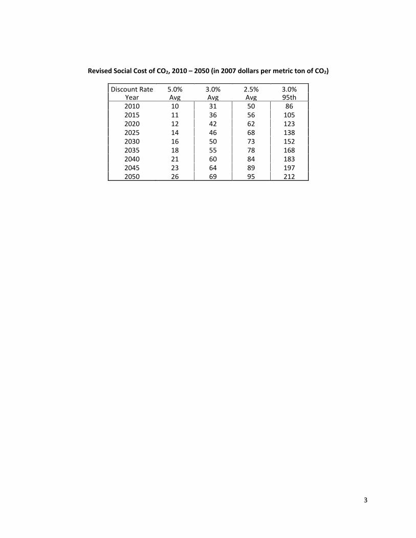
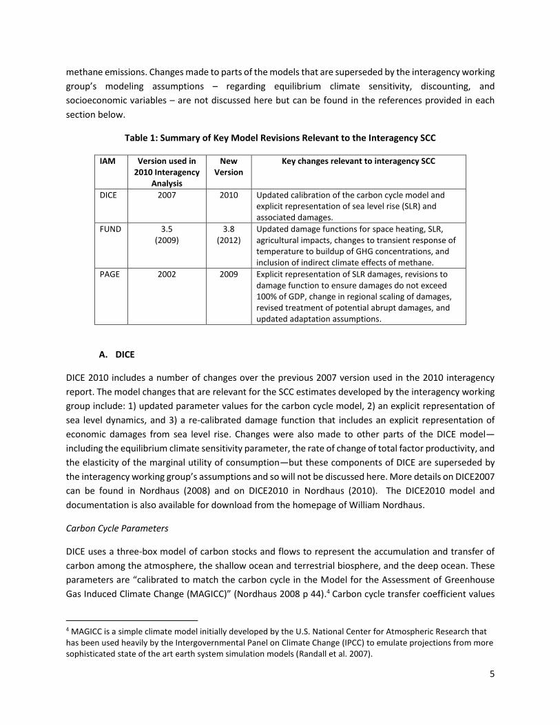
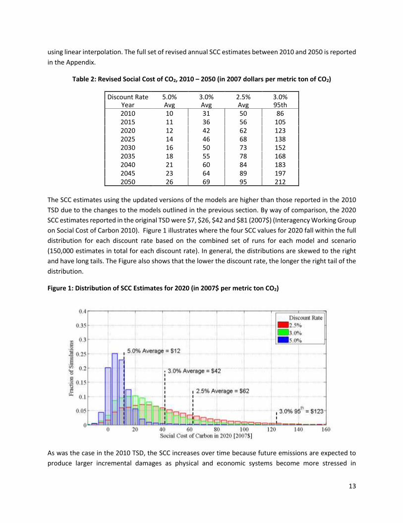
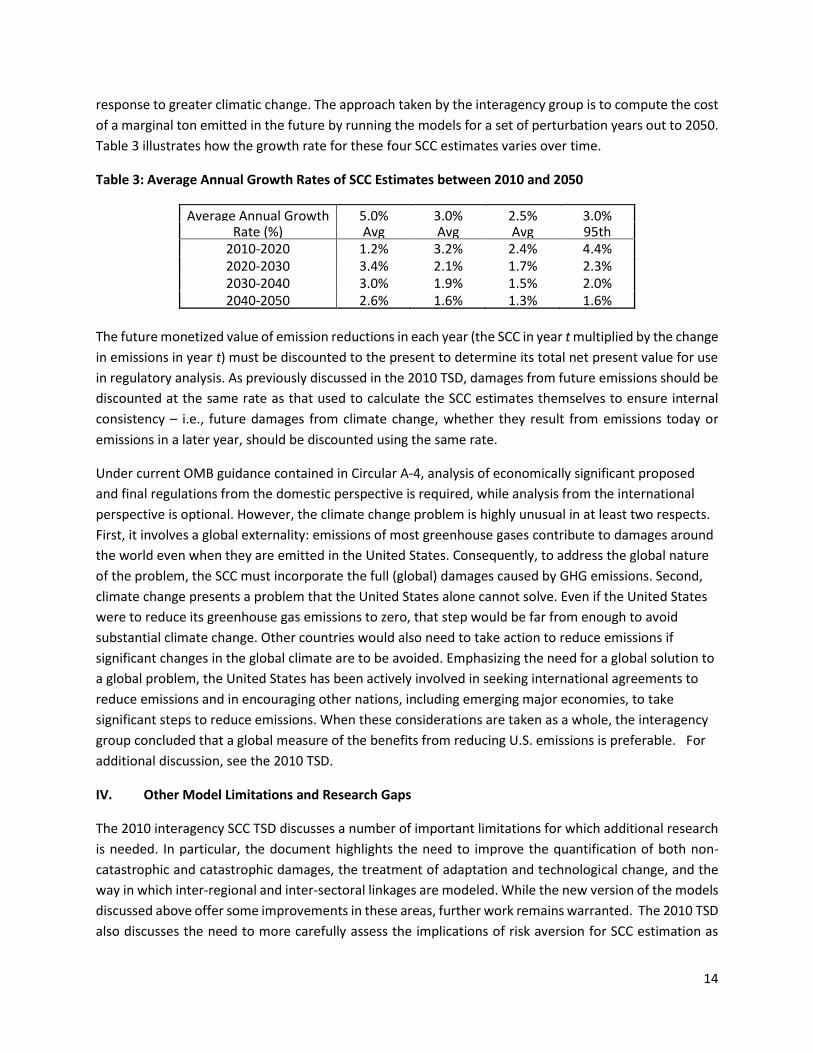
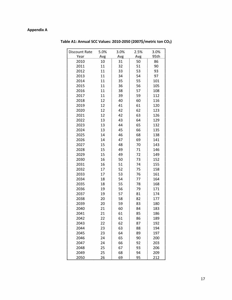
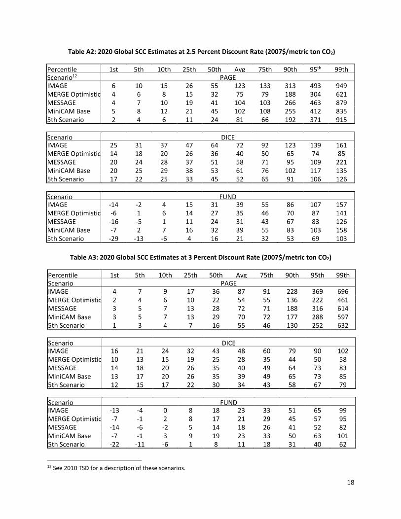
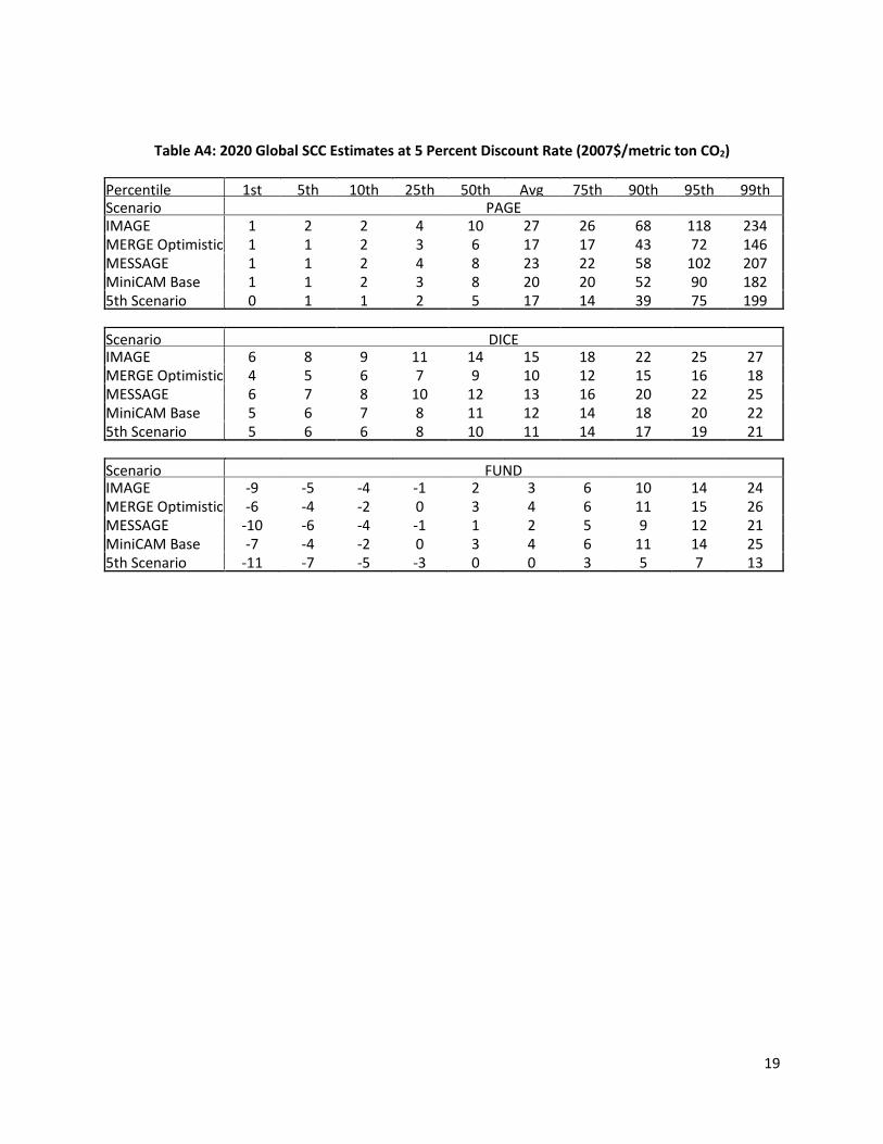
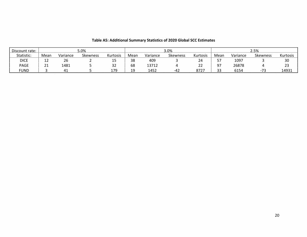