Technoeconomic Modeling of Battery Energy … lead-acid and lithium-ion battery models have been integrated with photovoltaic models giving System Advisor Model (SAM) the ability to

NREL is a national laboratory of the U.S. Department of Energy Office of Energy Efficiency & Renewable Energy Operated by the Alliance for Sustainable Energy, LLC This report is available at no cost from the National Renewable Energy Laboratory (NREL) at www.nrel.gov/publications.

Contract No. DE-AC36-08GO28308

Technoeconomic Modeling of Battery Energy Storage in SAM Nicholas DiOrio, Aron Dobos, Steven Janzou, Austin Nelson, and Blake Lundstrom National Renewable Energy Laboratory

Technical Report NREL/TP-6A20-64641 September 2015

NREL is a national laboratory of the U.S. Department of Energy Office of Energy Efficiency & Renewable Energy Operated by the Alliance for Sustainable Energy, LLC This report is available at no cost from the National Renewable Energy Laboratory (NREL) at www.nrel.gov/publications.

Contract No. DE-AC36-08GO28308

National Renewable Energy Laboratory 15013 Denver West Parkway Golden, CO 80401 303-275-

Technoeconomic Modeling of Battery Energy Storage in SAM Nicholas DiOrio, Aron Dobos, Steven Janzou, Austin Nelson, and Blake Lundstrom National Renewable Energy Laboratory

Prepared under Task No. SS13.9001

Technical Report NREL/TP-6A20-64641 September 2015

NOTICE

This report was prepared as an account of work sponsored by an agency of the United States government. Neither the United States government nor any agency thereof, nor any of their employees, makes any warranty, express or implied, or assumes any legal liability or responsibility for the accuracy, completeness, or usefulness of any information, apparatus, product, or process disclosed, or represents that its use would not infringe privately owned rights. Reference herein to any specific commercial product, process, or service by trade name, trademark, manufacturer, or otherwise does not necessarily constitute or imply its endorsement, recommendation, or favoring by the United States government or any agency thereof. The views and opinions of authors expressed herein do not necessarily state or reflect those of the United States government or any agency thereof.

This report is available at no cost from the National Renewable Energy Laboratory (NREL) at www.nrel.gov/publications.

Available electronically at SciTech Connect http:/www.osti.gov/scitech

Available for a processing fee to U.S. Department of Energy and its contractors, in paper, from:

U.S. Department of Energy Office of Scientific and Technical Information P.O. Box 62 Oak Ridge, TN 37831-0062 OSTI http://www.osti.gov Phone: 865.576.8401 Fax: 865.576.5728 Email: [email protected]

Available for sale to the public, in paper, from:

U.S. Department of Commerce National Technical Information Service 5301 Shawnee Road Alexandria, VA 22312 NTIS http://www.ntis.gov Phone: 800.553.6847 or 703.605.6000 Fax: 703.605.6900 Email: [email protected]

Cover Photos by Dennis Schroeder: (left to right) NREL 26173, NREL 18302, NREL 19758, NREL 29642, NREL 19795.

NREL prints on paper that contains recycled content.

http://www.osti.gov/scitech

http://www.osti.gov/

mailto:[email protected]

http://www.ntis.gov/

mailto:[email protected]

iii


Executive Summary Comprehensive lead-acid and lithium-ion battery models have been integrated with photovoltaic models giving System Advisor Model (SAM) the ability to predict the performance and economic benefit of behind the meter energy storage. In a system with storage, excess PV energy can be saved until later in the day when PV production has fallen, or until times of peak demand when it is more valuable. Complex dispatch strategies can be developed to leverage storage to reduce energy consumption or power demand based on the utility rate structure. This document describes the details of the battery performance and economic models in SAM.

1


1 Introduction SAM [1] links a high temporal resolution quasi-steady state PV-coupled battery energy storage performance model to detailed financial models to predict the economic performance of a system. The model was validated against existing models as well as physical testing of off-the-shelf battery equipment. A future paper will present case studies of systems with high penetrations of PV with and without distributed energy storage (DES) to evaluate the economic benefit of adding storage. Several performance sub-models of battery behavior had to be coherently integrated to provide a sufficiently realistic yet general interface for users of any type of lead-acid and lithium-ion battery. These models include a capacity model, voltage model, thermal model, and a lifetime model. Sensible dispatch strategies also had to be accommodated to allow users sufficient latitude in selecting how to use stored energy. Of primary importance is that users of the tool can find input parameters to the models on typical battery datasheets. The combined storage performance and dispatch models offer significant new capabilities to SAM which will assist interested parties with planning and evaluation of PV coupled with storage systems.

Ample literature is available describing mathematical battery models of varying complexity and scope. Battery models can be classified depending on the modeling approach. Bulk electrochemical models are well-suited to the purposes of SAM and typically can be characterized from the information on battery data sheets. These models seek only to describe aggregate quantities such as terminal voltage and battery charge.

Before describing the models chosen, it is worth commenting briefly on other types of battery models that were considered. Molecular level physics based electrochemical models provide a high level of fidelity but are unsuitable for the application due to their highly detailed input and runtime requirements. Empirical models, such as that developed for lead-acid batteries by Copetti [1] were not used due to their lack of generality. Other high level model types have been developed to characterize battery performance but suffer from requiring inputs not typically available on data sheets. Multiple types of battery chemistry beyond lithium-ion and lead-acid are under development or active in the market place [2], but are not considered here.

Common bulk electrochemical models are often based on work of Peukert [3], who modeled the relation between discharge current and capacity; and Shepard [4], who described the terminal voltage as a function of current, capacity, and charge state. For SAM the phenomenological approach of Manwell [5] was chosen to model the transient capacity and charge-transfer process in lead-acid systems. Lithium-ion batteries can charge and discharge more rapidly than lead-acid systems, and to model capacity in these batteries a simple tank-of-charge model was derived. Tremblay [6] extended the work of Shepard to provide a general dynamic voltage model across multiple battery chemistries, and was chosen to characterize terminal voltage for both chemistry types in SAM. The rainflow counting method described by Downing [7] is used to count battery charge/discharge cycles and coupled with manufacturer provided degradation curves permits an estimation of cycling capacity fade. Neubauer [8] described a thermal model for electric-vehicle batteries considering thermal radiation and cabin heat-transfer, which informed derivation of a simple heat-transfer model to predict battery temperature. Finally, a simple dispatch model was developed to provide a user with several options for how to effectively leverage their battery system.

2


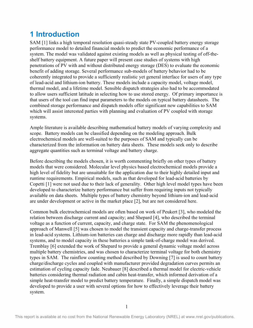
SAM currently assumes the battery is AC connected through a power converter, that is, it is in parallel with the load, grid, and PV system. The power conversion is approximated by two single point efficiencies, one upon power entering the battery for charging, and one as power leaves the battery for discharging. The efficiencies are applied to the current as in equation (1). = (1) = The charging efficiency is referred to as AC to DC efficiency, with the assumption that power is coming from an AC source. The discharging efficiency is referred to as DC to AC efficiency, with the assumption that DC power must be reinverted to meet an AC load. Other configurations exist, such as where power flows to the battery from a DC source (PV array) through one or two charge controllers, or power comes from an AC source, is inverted, and then sent through a charge controller to the battery. Figure 1 illustrates the modeled configuration.

Figure 1: Modeled configuration

Battery bank sizing can be done automatically by specifying desired bank capacity, voltage, cell capacity and voltage. Alternatively, a user can build a custom bank by defining how many cells should be connected in series and how many additional cells should be added in parallel. Cells added in parallel must be added in strings to maintain bank voltage. Figure 2 shows a battery with three parallel strings of four cells in series. As cells are added in series, bank voltage increases; as strings are added in parallel, capacity increases.

Figure 2: Example cell configuration

3


2 Generic Performance Models This section will describe performance models that are common to lead-acid and lithium-ion battery chemistries. Specifically, a general voltage model, thermal model and cycle counting method will be detailed.

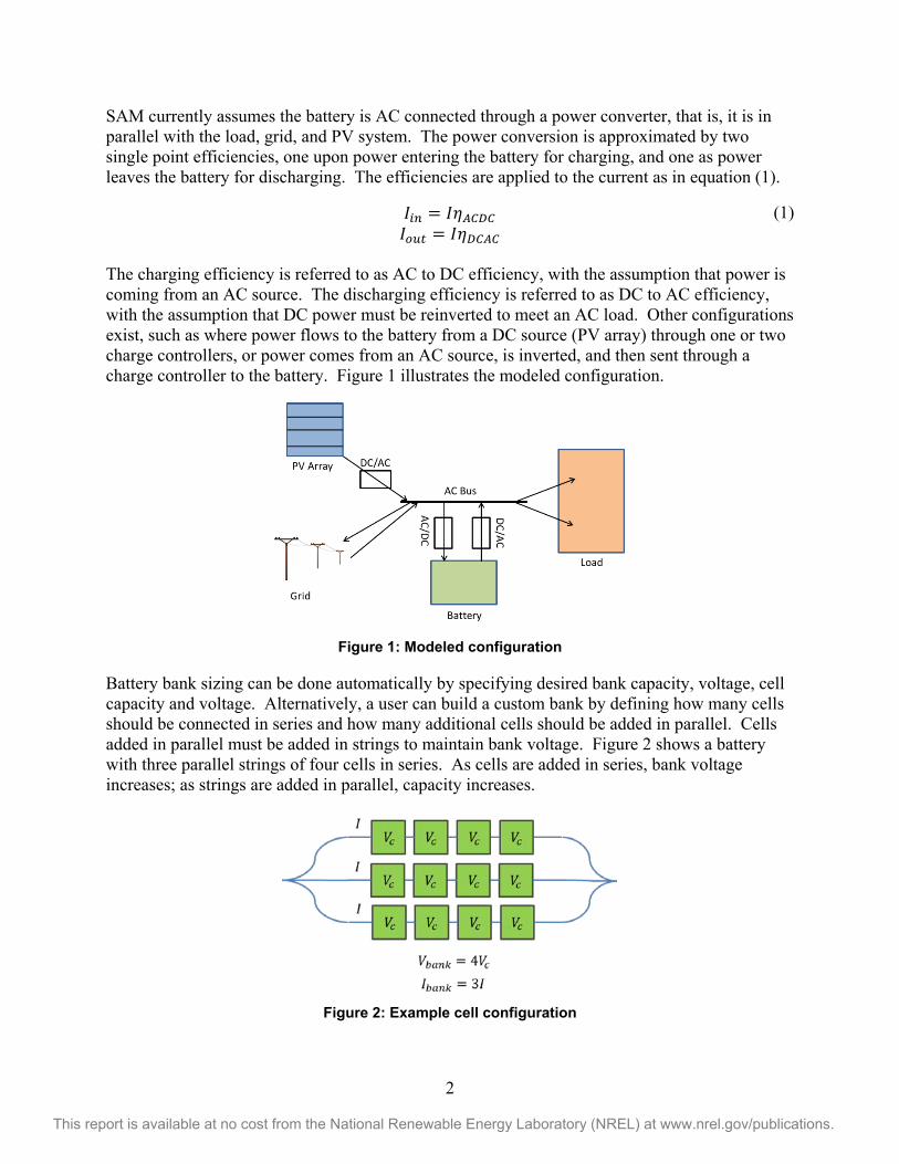
2. 1 Voltage Model Battery terminal voltage varies as a function of current, capacity, state-of-charge, and other factors requiring a dynamic model to characterize the voltage at a given time. The voltage model does not consider temperature effects as manufacturer data sheets do not commonly list voltage-vs-temperature information. The voltage model indirectly incorporates temperature effects through the battery capacity, which is coupled with the thermal model. The model treats charging and discharging modes in the same way. The dynamic voltage model is a generic electrochemical model based on [6]. Model parameters are based on extracted parameters from battery datasheets. The voltage model is given by Equation (1) and Table 1.

= +

(2)

Table 1: Voltage model variables

Variable Description Terminal voltage (V) Battery constant voltage (V) Polarization voltage (V)

Battery capacity (Ah) Actual battery charge (Ah) Exponential zone amplitude (V) Exponential zone time constant inverse (Ah)-1

Internal resistance ( ) Battery current (A) Time step (hr)

is an expression for how much capacity has been removed and can be computed as in

Equation (2). = (3)

V0, K, a, and B are parameters from manufacturer voltage vs. charge-removed curves. 2.1.1 Parameter determination A voltage discharge curve for a battery cell must be used to determine the constants required by the voltage model as described in [6].

4


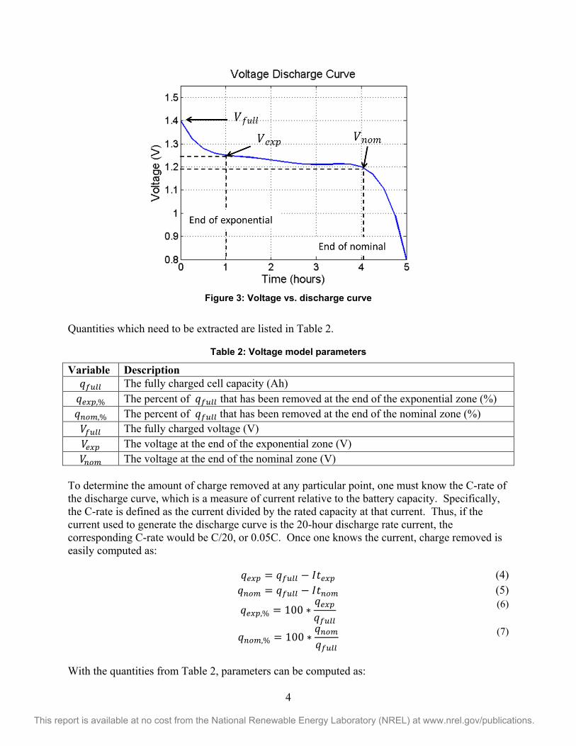
Figure 3: Voltage vs. discharge curve

Quantities which need to be extracted are listed in Table 2.

Table 2: Voltage model parameters

Variable Description The fully charged cell capacity (Ah)

,% The percent of that has been removed at the end of the exponential zone (%) ,% The percent of that has been removed at the end of the nominal zone (%) The fully charged voltage (V) The voltage at the end of the exponential zone (V) The voltage at the end of the nominal zone (V)

To determine the amount of charge removed at any particular point, one must know the C-rate of the discharge curve, which is a measure of current relative to the battery capacity. Specifically, the C-rate is defined as the current divided by the rated capacity at that current. Thus, if the current used to generate the discharge curve is the 20-hour discharge rate current, the corresponding C-rate would be C/20, or 0.05C. Once one knows the current, charge removed is easily computed as:

= (4) = (5)

,% = 100 (6)

,% = 100 (7)

With the quantities from Table 2, parameters can be computed as:

5


= (8)

=3

(9)

=+ ( 1) ( )

(10)

= + + (11) 2.1.2 Model limitations The voltage model attempts to describe a voltage discharge curve over a wide range of charge states, including the portion of the voltage curve which is highly non-linear. At regions of very low state-of-charge (less than 1%), the model becomes undefined. If the battery is simulated allowing extremely low states-of-charge and the voltage becomes negative or undefined the model will return the voltage value as half the nominal voltage. Furthermore, if the battery is overcharged and terminal voltage exceeds the full cell voltage by more than 125%, the voltage will be limited to the full cell voltage. These limits are arbitrary and exist solely to avoid undefined behavior.

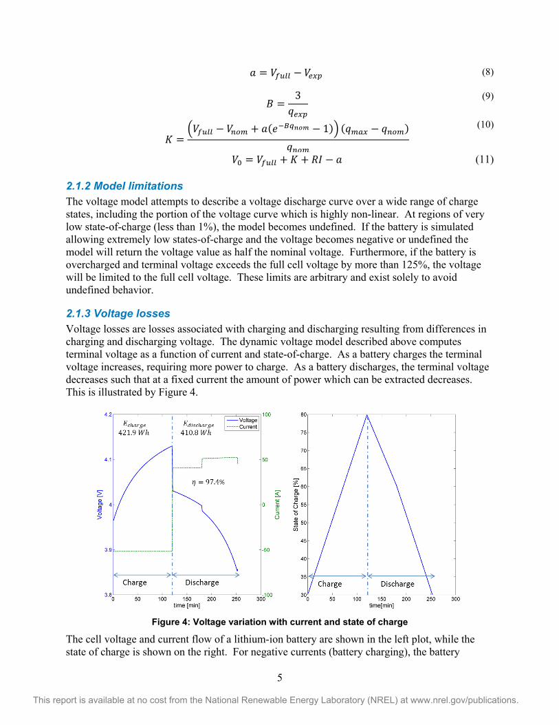
2.1.3 Voltage losses Voltage losses are losses associated with charging and discharging resulting from differences in charging and discharging voltage. The dynamic voltage model described above computes terminal voltage as a function of current and state-of-charge. As a battery charges the terminal voltage increases, requiring more power to charge. As a battery discharges, the terminal voltage decreases such that at a fixed current the amount of power which can be extracted decreases. This is illustrated by Figure 4.

Figure 4: Voltage variation with current and state of charge

The cell voltage and current flow of a lithium-ion battery are shown in the left plot, while the state of charge is shown on the right. For negative currents (battery charging), the battery

6


voltage increases. For positive currents (battery discharging), the cell voltage decreases. As the figure demonstrates, more energy is required to charge from 30% SOC to 80% SOC than can be extracted over the same range. This leads to the concept of round-trip efficiency.

2.1.4 Round-trip efficiency At every time step, the energy sent to charge the battery or energy discharged from the battery is recorded. The efficiency is the total amount of energy discharged over all timesteps divided by the total amount of energy required to charge over all timesteps. The energy is computed after all losses are applied by computing:

= 0.5 ( + ) (12) Where I is the current, is the voltage at the end of the timestep, and is the voltage at the beginning of the timestep. If E is greater than 0, the energy over the timestep is added to , the accumulated energy discharged. If E is less than 0, the energy over the timestep is added to , the accumulated energy charged. At the end of the simulation, the round-trip efficiency is computed as in Equation (12).

= 100 ( ) (13)

This efficiency is sensitive to the average charging and discharging current. As this average increases, thermal losses increase and reduce the efficiency.

2.2 Thermal Model Thermal effects are important to battery performance, because the battery temperature directly affects its capacity and lifetime. Typically, battery capacity drops as the temperature decreases and increases as temperature increases. Excessively high temperatures result in corrosion and a significant reduction in lifetime. Therefore accurate representation of quantities of economic importance requires effective modeling of battery temperature. Many system configurations are possible; however, only a simple scenario where the battery is placed in a conditioned room of fixed temperature is considered. More general scenarios involve configurations exposing the battery to ambient weather conditions, which may result in suboptimal performance and lifetime. The system configuration studied is seen in Figure 5 .

7


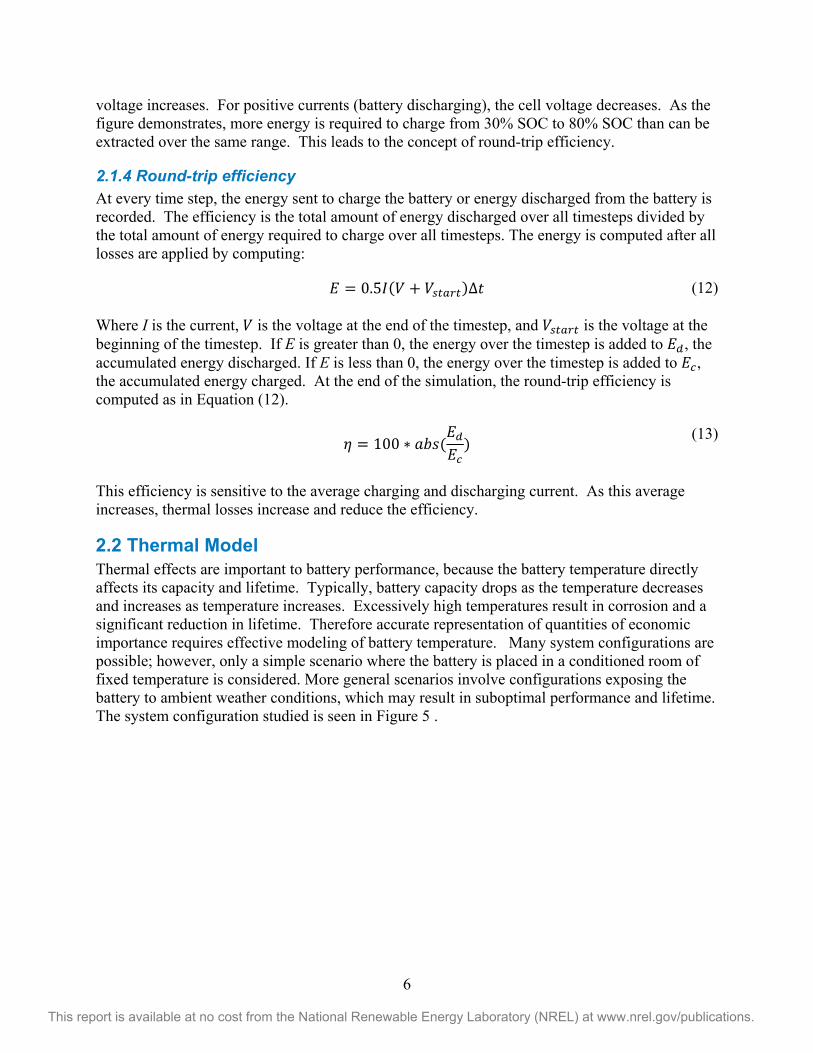
Figure 5: Thermal model system configuration

The user can specify several properties describing the thermal characteristics of the battery. The model is an energy balance of thermal storage within the battery, heat transfer to and from the room, and heat generation due to internal resistance. The differential equation describing the heat transfer was derived from an energy balance on the battery system. The quantity of interest is the battery temperature. No incident radiation is considered.

( ) = =

( ) +

(14)

To mitigate stability issues, the second-order, unconditionally stable trapezoidal method is used to numerically step the temperature forward in time. The implicit method takes the form:

, = , +

2[ , + ( , )] (15)

The output of the thermal model is the bulk average temperature of the battery, which is then used to compute the relative capacity based on a lookup table of relative capacity with temperature. Thermal effects on battery lifetime are not considered. The current discharge and charge rate are the primary terms influencing thermal losses and battery efficiency. To improve battery efficiency, the user can tailor the maximum current rates to reduce thermal losses. Without limiting current discharge battery efficiency will noticeably decrease, particularly at sub-hourly time-steps. Battery mass and surface area are input as units per energy, so that adjusting the size of the battery bank results in dynamic scaling of mass and area.

The user enters information about capacity versus temperature to apply thermal losses. Losses are applied to the amount of charge in the battery. The capacity modifier is a percent of how much loss applies at a given temperature. The loss is applied to the capacity as:

= 0.01 (16)

8


2.3 Lifetime Model Lithium-ion and lead-acid batteries have calendar and cycle-dependent characteristics. Lead-acid battery data sheets typically report capacity degradation, depending on how many cycles have elapsed at an average depth-of-discharge (DoD), whereas lithium-ion battery data sheets often report the capacity degradation at a given number of cycles. To track the number of cycles that a battery has undergone, a rainflow counting algorithm [7] is applied. This provides a means to distill a complex, irregular discharge history into a series of constant amplitude events.

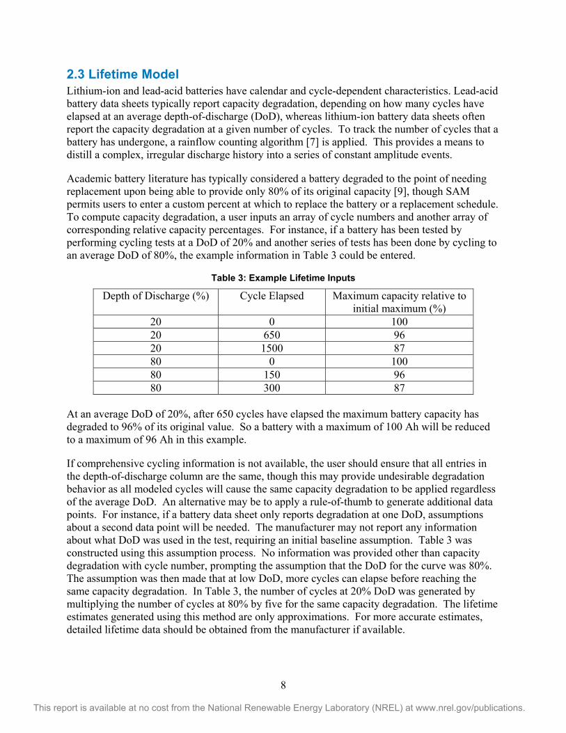
Academic battery literature has typically considered a battery degraded to the point of needing replacement upon being able to provide only 80% of its original capacity [9], though SAM permits users to enter a custom percent at which to replace the battery or a replacement schedule. To compute capacity degradation, a user inputs an array of cycle numbers and another array of corresponding relative capacity percentages. For instance, if a battery has been tested by performing cycling tests at a DoD of 20% and another series of tests has been done by cycling to an average DoD of 80%, the example information in Table 3 could be entered.

Table 3: Example Lifetime Inputs

Depth of Discharge (%) Cycle Elapsed Maximum capacity relative to initial maximum (%)

20 0 100 20 650 96 20 1500 87 80 0 100 80 150 96 80 300 87

At an average DoD of 20%, after 650 cycles have elapsed the maximum battery capacity has degraded to 96% of its original value. So a battery with a maximum of 100 Ah will be reduced to a maximum of 96 Ah in this example.

If comprehensive cycling information is not available, the user should ensure that all entries in the depth-of-discharge column are the same, though this may provide undesirable degradation behavior as all modeled cycles will cause the same capacity degradation to be applied regardless of the average DoD. An alternative may be to apply a rule-of-thumb to generate additional data points. For instance, if a battery data sheet only reports degradation at one DoD, assumptions about a second data point will be needed. The manufacturer may not report any information about what DoD was used in the test, requiring an initial baseline assumption. Table 3 was constructed using this assumption process. No information was provided other than capacity degradation with cycle number, prompting the assumption that the DoD for the curve was 80%. The assumption was then made that at low DoD, more cycles can elapse before reaching the same capacity degradation. In Table 3, the number of cycles at 20% DoD was generated by multiplying the number of cycles at 80% by five for the same capacity degradation. The lifetime estimates generated using this method are only approximations. For more accurate estimates, detailed lifetime data should be obtained from the manufacturer if available.

9


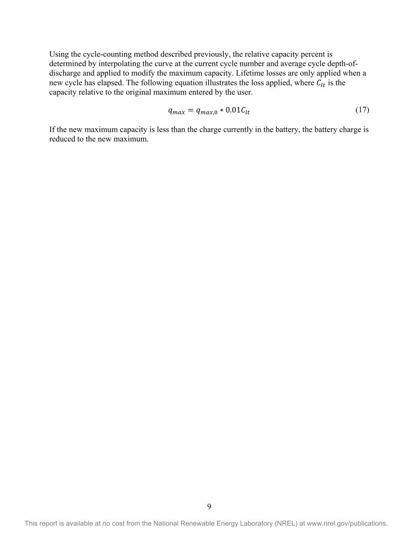
Using the cycle-counting method described previously, the relative capacity percent is determined by interpolating the curve at the current cycle number and average cycle depth-of-discharge and applied to modify the maximum capacity. Lifetime losses are only applied when a new cycle has elapsed. The following equation illustrates the loss applied, where is the capacity relative to the original maximum entered by the user.

= , 0.01 (17) If the new maximum capacity is less than the charge currently in the battery, the battery charge is reduced to the new maximum.

10


3 Lead Acid Performance Models 3. 1 Capacity Model Lead-acid batteries exhibit certain characteristics which distinguish them from other batteries.

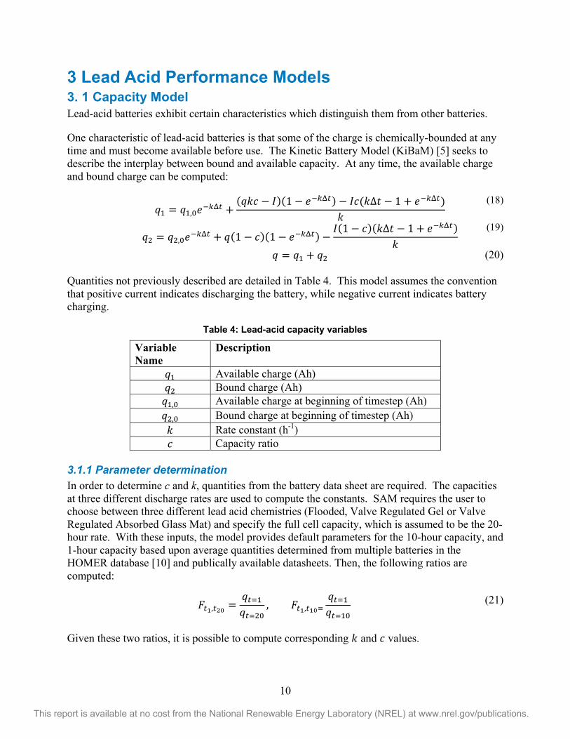
One characteristic of lead-acid batteries is that some of the charge is chemically-bounded at any time and must become available before use. The Kinetic Battery Model (KiBaM) [5] seeks to describe the interplay between bound and available capacity. At any time, the available charge and bound charge can be computed:

= , +

( )(1 ) ( 1 + )

(18)

= , + (1 )(1 )

(1 )( 1 + )

(19)

= + (20) Quantities not previously described are detailed in Table 4. This model assumes the convention that positive current indicates discharging the battery, while negative current indicates battery charging.

Table 4: Lead-acid capacity variables

Variable Name

Description

Available charge (Ah) Bound charge (Ah)

, Available charge at beginning of timestep (Ah) , Bound charge at beginning of timestep (Ah) Rate constant (h-1) Capacity ratio

3.1.1 Parameter determination In order to determine c and k, quantities from the battery data sheet are required. The capacities at three different discharge rates are used to compute the constants. SAM requires the user to choose between three different lead acid chemistries (Flooded, Valve Regulated Gel or Valve Regulated Absorbed Glass Mat) and specify the full cell capacity, which is assumed to be the 20-hour rate. With these inputs, the model provides default parameters for the 10-hour capacity, and 1-hour capacity based upon average quantities determined from multiple batteries in the HOMER database [10] and publically available datasheets. Then, the following ratios are computed:

, = , , (21)

Given these two ratios, it is possible to compute corresponding and values.

11


=

(1 ) (1 )(1 ) (1 ) +

(22)

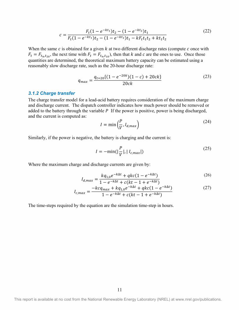
When the same is obtained for a given at two different discharge rates (compute once with

= , , the next time with = , ), then that and are the ones to use. Once those quantities are determined, the theoretical maximum battery capacity can be estimated using a reasonably slow discharge rate, such as the 20-hour discharge rate:

={(1 )(1 ) + 20 }

20

(23)

3.1.2 Charge transfer The charge transfer model for a lead-acid battery requires consideration of the maximum charge and discharge current. The dispatch controller indicates how much power should be removed or added to the battery through the variable If the power is positive, power is being discharged, and the current is computed as: = min , , (24)

Similarly, if the power is negative, the battery is charging and the current is: = min (| |, | , |) (25)

Where the maximum charge and discharge currents are given by:

, = , + (1 )1 + ( 1 + )

(26)

, =+ , + (1 )

1 + ( 1 + )

(27)

The time-steps required by the equation are the simulation time-step in hours.

12


4 Lithium-ion Performance Models Lithium-ion batteries are capable of discharging more rapidly and deeply than lead-acid batteries, making the capacity model substantially different. 4.1 Default Chemistries A set of lithium-ion cell types are included to populate typical voltage curve and lifetime degradation defaults. [2] Default values are provided for the following lithium-ion cathodes coupled with a graphite or hard carbon anode: Nickel Manganese Cobalt Oxide (NMC), Nickel Cobalt Aluminum Oxide (NCA), Lithium Manganese Oxide (LMO), Lithium Iron Phosphate (LFP), Lithium Cobalt Oxide (LCO). Defaults are also provided for LMO as a cathode and Lithium Titanate (LTO) as an anode. Changing between lithium-ion chemistry types simply changes default values in the user interface and does not change underlying equations. Cells properties can vary markedly between manufacturers and product lines such that the default values do not capture the properties of a particular cell. The user is encouraged to use the defaults as a starting point and tailor model inputs as needed. 4.2 Capacity Model The lithium-ion capacity model treats the battery as a tank of charge, removing and adding charge as needed according to the following relation, again assuming that positive current implies discharging from the battery. = (28) The battery is only allowed to discharge to the user-specified minimum state-of-charge and stays within user-specified rates of current charge and discharge. Capacity relates to battery energy through the voltage. = (29) Power relates to battery energy by calculating how much energy is transferred over a period of time. = = =

(30)

The model computes voltage according to (2), which utilizes a static resistance.

13


5 Storage Dispatch SAM currently allows for a manual dispatch strategy, where the user can set up custom profiles and then schedule those profiles on a month by month, hour by hour schedule throughout the year. This tool allows the user to specify detailed characteristics, such as when to allow discharging, how much of the capacity to discharge, and the minimum state-of-charge. With these detailed options, the user can choose how to dispatch storage in the hours offering the most benefit.

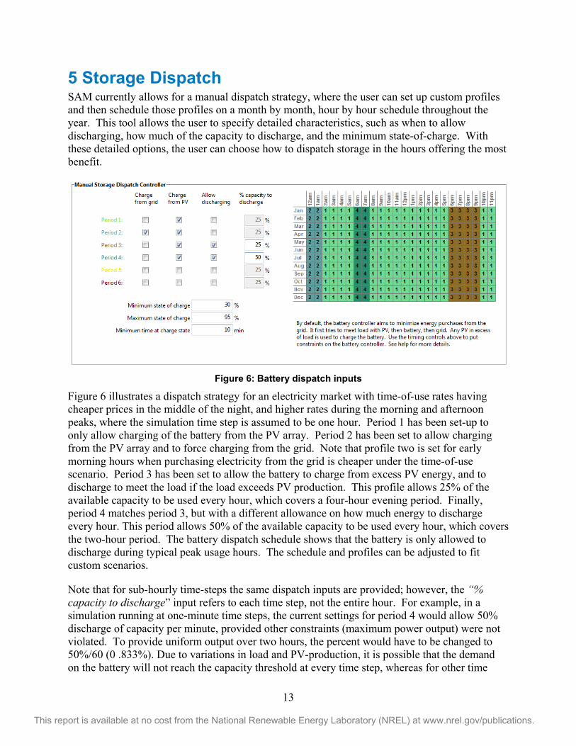
Figure 6: Battery dispatch inputs

Figure 6 illustrates a dispatch strategy for an electricity market with time-of-use rates having cheaper prices in the middle of the night, and higher rates during the morning and afternoon peaks, where the simulation time step is assumed to be one hour. Period 1 has been set-up to only allow charging of the battery from the PV array. Period 2 has been set to allow charging from the PV array and to force charging from the grid. Note that profile two is set for early morning hours when purchasing electricity from the grid is cheaper under the time-of-use scenario. Period 3 has been set to allow the battery to charge from excess PV energy, and to discharge to meet the load if the load exceeds PV production. This profile allows 25% of the available capacity to be used every hour, which covers a four-hour evening period. Finally, period 4 matches period 3, but with a different allowance on how much energy to discharge every hour. This period allows 50% of the available capacity to be used every hour, which covers the two-hour period. The battery dispatch schedule shows that the battery is only allowed to discharge during typical peak usage hours. The schedule and profiles can be adjusted to fit custom scenarios.

Note that for sub-hourly time-steps the same dispatch inputs are provided; however, the “% capacity to discharge” input refers to each time step, not the entire hour. For example, in a simulation running at one-minute time steps, the current settings for period 4 would allow 50% discharge of capacity per minute, provided other constraints (maximum power output) were not violated. To provide uniform output over two hours, the percent would have to be changed to 50%/60 (0 .833%). Due to variations in load and PV-production, it is possible that the demand on the battery will not reach the capacity threshold at every time step, whereas for other time

14


steps the demand may exceed the threshold, leading to under-utilization of the battery. At sub-hourly time steps it may thus be desirable to double or quadruple the discharge percent to allow for variations in battery demand with the understanding that this will allow more of the battery capacity to be used (up to the minimum state-of-charge), but may also result in the battery not contributing energy during later portions of the period.

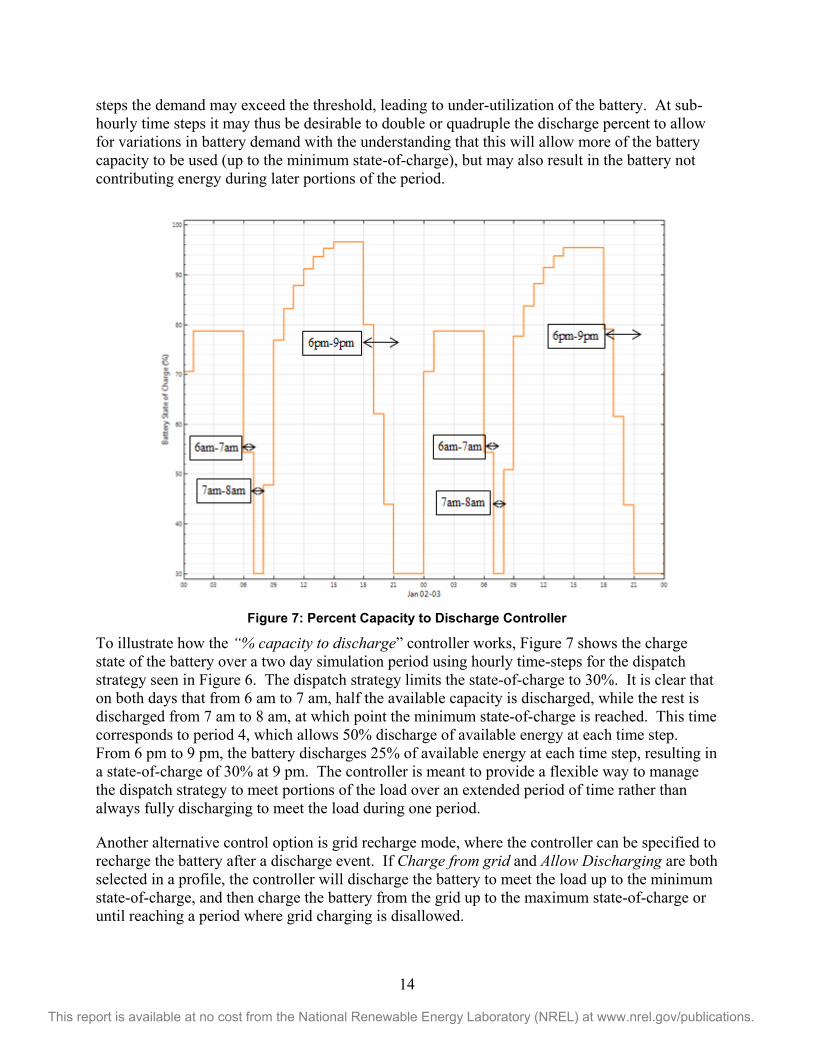
Figure 7: Percent Capacity to Discharge Controller

To illustrate how the “% capacity to discharge” controller works, Figure 7 shows the charge state of the battery over a two day simulation period using hourly time-steps for the dispatch strategy seen in Figure 6. The dispatch strategy limits the state-of-charge to 30%. It is clear that on both days that from 6 am to 7 am, half the available capacity is discharged, while the rest is discharged from 7 am to 8 am, at which point the minimum state-of-charge is reached. This time corresponds to period 4, which allows 50% discharge of available energy at each time step. From 6 pm to 9 pm, the battery discharges 25% of available energy at each time step, resulting in a state-of-charge of 30% at 9 pm. The controller is meant to provide a flexible way to manage the dispatch strategy to meet portions of the load over an extended period of time rather than always fully discharging to meet the load during one period.

Another alternative control option is grid recharge mode, where the controller can be specified to recharge the battery after a discharge event. If Charge from grid and Allow Discharging are both selected in a profile, the controller will discharge the battery to meet the load up to the minimum state-of-charge, and then charge the battery from the grid up to the maximum state-of-charge or until reaching a period where grid charging is disallowed.

15


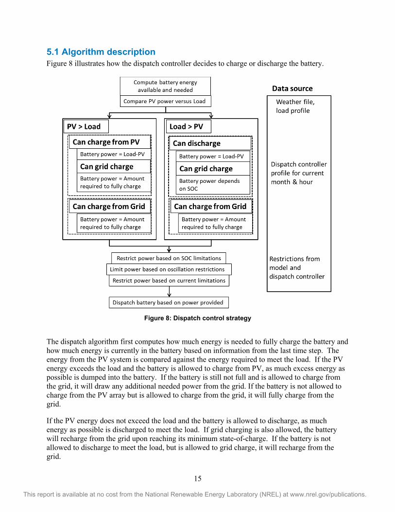
5.1 Algorithm description Figure 8 illustrates how the dispatch controller decides to charge or discharge the battery.

Figure 8: Dispatch control strategy

The dispatch algorithm first computes how much energy is needed to fully charge the battery and how much energy is currently in the battery based on information from the last time step. The energy from the PV system is compared against the energy required to meet the load. If the PV energy exceeds the load and the battery is allowed to charge from PV, as much excess energy as possible is dumped into the battery. If the battery is still not full and is allowed to charge from the grid, it will draw any additional needed power from the grid. If the battery is not allowed to charge from the PV array but is allowed to charge from the grid, it will fully charge from the grid.

If the PV energy does not exceed the load and the battery is allowed to discharge, as much energy as possible is discharged to meet the load. If grid charging is also allowed, the battery will recharge from the grid upon reaching its minimum state-of-charge. If the battery is not allowed to discharge to meet the load, but is allowed to grid charge, it will recharge from the grid.

16


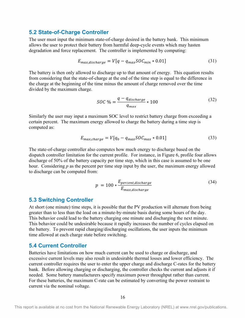
5.2 State-of-Charge Controller The user must input the minimum state-of-charge desired in the battery bank. This minimum allows the user to protect their battery from harmful deep-cycle events which may hasten degradation and force replacement. The controller is implemented by computing:

, = [ 0.01]

(31)

The battery is then only allowed to discharge up to that amount of energy. This equation results from considering that the state-of-charge at the end of the time step is equal to the difference in the charge at the beginning of the time minus the amount of charge removed over the time divided by the maximum charge.

% = 100 (32)

Similarly the user may input a maximum SOC level to restrict battery charge from exceeding a certain percent. The maximum energy allowed to charge the battery during a time step is computed as:

, = [ 0.01]

(33)

The state-of-charge controller also computes how much energy to discharge based on the dispatch controller limitation for the current profile. For instance, in Figure 6, profile four allows discharge of 50% of the battery capacity per time step, which in this case is assumed to be one hour. Considering p as the percent per time step input by the user, the maximum energy allowed to discharge can be computed from:

= 100 ,

,

(34)

5.3 Switching Controller At short (one minute) time steps, it is possible that the PV production will alternate from being greater than to less than the load on a minute-by-minute basis during some hours of the day. This behavior could lead to the battery charging one minute and discharging the next minute. This behavior could be undesirable because it rapidly increases the number of cycles elapsed on the battery. To prevent rapid charging/discharging oscillations, the user inputs the minimum time allowed at each charge state before switching.

5.4 Current Controller Batteries have limitations on how much current can be used to charge or discharge, and excessive current levels may also result in undesirable thermal losses and lower efficiency. The current controller requires the user to enter the upper charge and discharge C-rates for the battery bank. Before allowing charging or discharging, the controller checks the current and adjusts it if needed. Some battery manufacturers specify maximum power throughput rather than current. For these batteries, the maximum C-rate can be estimated by converting the power restraint to current via the nominal voltage.

17


6 Battery Economics SAM includes a powerful new feature which allows simulation over the entire analysis period rather than extending the first-year analysis to future years. The feature was introduced to capture the variable nature of battery replacements, which depend heavily on their cycling behavior. As a battery degrades beyond a certain point, its use as a stationary storage device becomes limited and the battery must be replaced. This introduces potentially large capital replacement costs into the financial analysis which must be considered to evaluate the economic impact of adding batteries to a system over the system lifetime.

Users can specify whether to replace the battery and at what capacity degradation percent the battery should be replaced. Alternatively a user can enter a replacement schedule which details in which years the battery bank should be replaced. In addition, battery bank replacement costs can be entered either as a fixed $/kWh value, or as a schedule over time. Escalation costs can be input to explore increasing or decreasing battery costs relative to inflation over time.

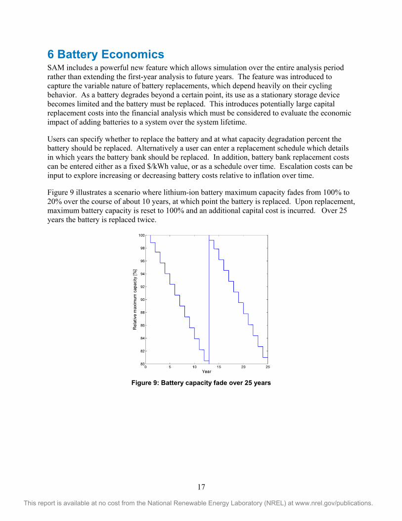
Figure 9 illustrates a scenario where lithium-ion battery maximum capacity fades from 100% to 20% over the course of about 10 years, at which point the battery is replaced. Upon replacement, maximum battery capacity is reset to 100% and an additional capital cost is incurred. Over 25 years the battery is replaced twice.

Figure 9: Battery capacity fade over 25 years

18


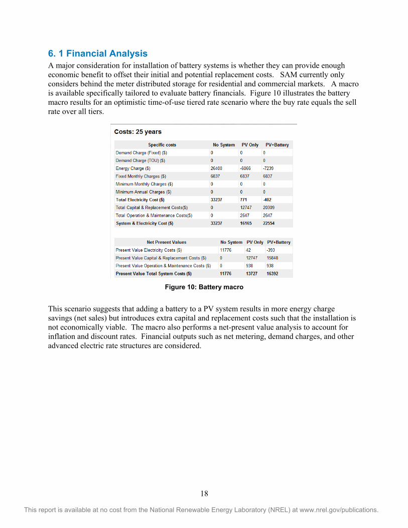
6. 1 Financial Analysis A major consideration for installation of battery systems is whether they can provide enough economic benefit to offset their initial and potential replacement costs. SAM currently only considers behind the meter distributed storage for residential and commercial markets. A macro is available specifically tailored to evaluate battery financials. Figure 10 illustrates the battery macro results for an optimistic time-of-use tiered rate scenario where the buy rate equals the sell rate over all tiers.

Figure 10: Battery macro

This scenario suggests that adding a battery to a PV system results in more energy charge savings (net sales) but introduces extra capital and replacement costs such that the installation is not economically viable. The macro also performs a net-present value analysis to account for inflation and discount rates. Financial outputs such as net metering, demand charges, and other advanced electric rate structures are considered.

19


7 Model Validation Several validation approaches were taken to ensure the component-level models behave as anticipated. These approaches include comparing results with other software packages using similar models and comparing against experimental data. The software packages considered do not provide thermal or lifetime modeling capabilities. Experimental lifetime validation was not performed due to the prohibitive expense in performing lifetime cycling tests. It is the user’s responsibility to specify the capacity fade with cycling at various depths of discharge, which the model then applies.

7.1 HOMER comparison The HOMER Legacy tool (v2.28 beta) developed by HOMER Energy LLC provides the ability to model grid-connected renewable energy systems including lead-acid batteries and was used for comparison. Newer versions of HOMER have since been developed and released, and this comparison refers only to results obtained by HOMER Legacy. The HOMER Legacy lead-acid capacity model also uses KIBAM.

The simulated system was placed in Phoenix, AZ. Each model used the same load profile. A Universal Power Group UBGC2 sealed lead-acid AGM battery was used for comparison. There was difficulty in perfectly matching the dispatch profiles between models, as HOMER performs optimized dispatch based on specified criteria, whereas SAM dispatches based on user-specified schedules. Despite these differences, the dispatch strategies were tailored to match as closely as possible. The first comparison done used the full SAM battery model, including lifetime capacity fade, voltage, and thermal effects. The HOMER model appears to incorporate terminal voltage variation via an efficiency input within the battery, which was specified as 88%. HOMER does not include thermal modeling and does not appear to include lifetime capacity fade with cycling.

Of particular interest for the comparison was how much energy each model predicted being sent to the battery from the PV system, and how much energy went from the battery to meet the electric load. Of further interest was the charge state of the battery over time. Table 5 shows the battery energy quantities for each model, including a model of SAM where some features have been turned off.

Table 5: SAM vs. HOMER battery energy

SAM (Full Model)

SAM (Reduced Model)

HOMER

Energy to charge battery (kWh) 297.20 393.17 383.59 Energy discharged to load (kWh) 260.90 347.88 338.56 Battery efficiency (%) 87.79 88.48 88.26

The full SAM model predicts that less about 23% less energy goes to and from the battery compared to HOMER yet closely approximates the battery efficiency, computed from Eq. (12). The root-mean-square error (RMSE) for the battery SOC between the two models was 8.62%. The root mean square error was computed from Eq. (34).

20


= , ,

(35)

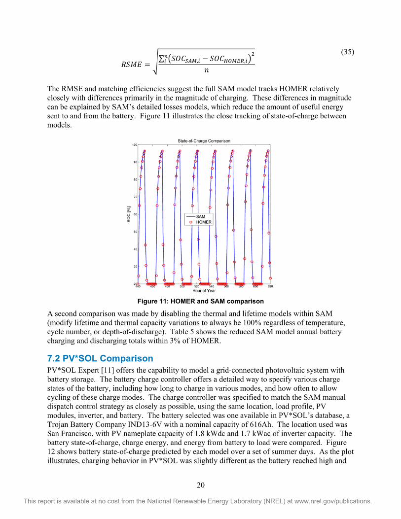
The RMSE and matching efficiencies suggest the full SAM model tracks HOMER relatively closely with differences primarily in the magnitude of charging. These differences in magnitude can be explained by SAM’s detailed losses models, which reduce the amount of useful energy sent to and from the battery. Figure 11 illustrates the close tracking of state-of-charge between models.

Figure 11: HOMER and SAM comparison

A second comparison was made by disabling the thermal and lifetime models within SAM (modify lifetime and thermal capacity variations to always be 100% regardless of temperature, cycle number, or depth-of-discharge). Table 5 shows the reduced SAM model annual battery charging and discharging totals within 3% of HOMER.

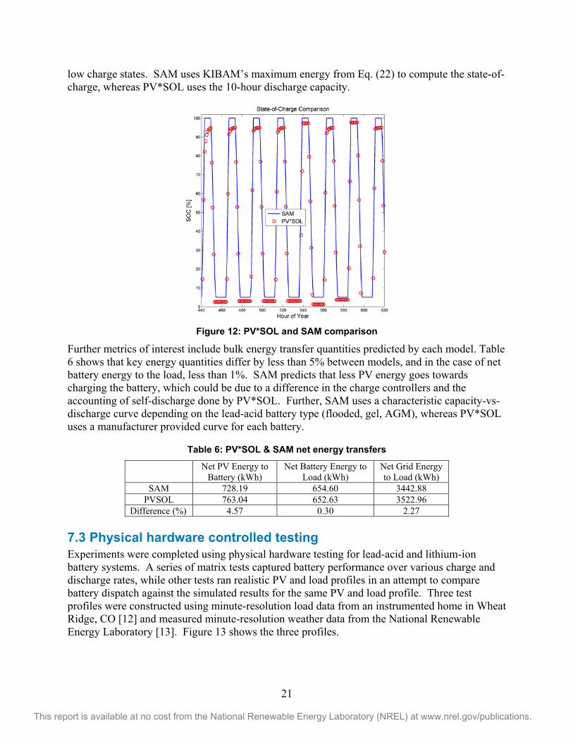
7.2 PV*SOL Comparison PV*SOL Expert [11] offers the capability to model a grid-connected photovoltaic system with battery storage. The battery charge controller offers a detailed way to specify various charge states of the battery, including how long to charge in various modes, and how often to allow cycling of these charge modes. The charge controller was specified to match the SAM manual dispatch control strategy as closely as possible, using the same location, load profile, PV modules, inverter, and battery. The battery selected was one available in PV*SOL’s database, a Trojan Battery Company IND13-6V with a nominal capacity of 616Ah. The location used was San Francisco, with PV nameplate capacity of 1.8 kWdc and 1.7 kWac of inverter capacity. The battery state-of-charge, charge energy, and energy from battery to load were compared. Figure 12 shows battery state-of-charge predicted by each model over a set of summer days. As the plot illustrates, charging behavior in PV*SOL was slightly different as the battery reached high and

21


low charge states. SAM uses KIBAM’s maximum energy from Eq. (22) to compute the state-of-charge, whereas PV*SOL uses the 10-hour discharge capacity.

Figure 12: PV*SOL and SAM comparison

Further metrics of interest include bulk energy transfer quantities predicted by each model. Table 6 shows that key energy quantities differ by less than 5% between models, and in the case of net battery energy to the load, less than 1%. SAM predicts that less PV energy goes towards charging the battery, which could be due to a difference in the charge controllers and the accounting of self-discharge done by PV*SOL. Further, SAM uses a characteristic capacity-vs-discharge curve depending on the lead-acid battery type (flooded, gel, AGM), whereas PV*SOL uses a manufacturer provided curve for each battery.

Table 6: PV*SOL & SAM net energy transfers

Net PV Energy to Battery (kWh)

Net Battery Energy to Load (kWh)

Net Grid Energy to Load (kWh)

SAM 728.19 654.60 3442.88 PVSOL 763.04 652.63 3522.96

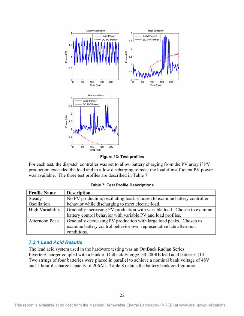
Difference (%) 4.57 0.30 2.27 7.3 Physical hardware controlled testing Experiments were completed using physical hardware testing for lead-acid and lithium-ion battery systems. A series of matrix tests captured battery performance over various charge and discharge rates, while other tests ran realistic PV and load profiles in an attempt to compare battery dispatch against the simulated results for the same PV and load profile. Three test profiles were constructed using minute-resolution load data from an instrumented home in Wheat Ridge, CO [12] and measured minute-resolution weather data from the National Renewable Energy Laboratory [13]. Figure 13 shows the three profiles.

22


Figure 13: Test profiles

For each test, the dispatch controller was set to allow battery charging from the PV array if PV production exceeded the load and to allow discharging to meet the load if insufficient PV power was available. The three test profiles are described in Table 7.

Table 7: Test Profile Descriptions

Profile Name Description Steady Oscillation

No PV production, oscillating load. Chosen to examine battery controller behavior while discharging to meet electric load.

High Variability Gradually increasing PV production with variable load. Chosen to examine battery control behavior with variable PV and load profiles.

Afternoon Peak Gradually decreasing PV production with large load peaks. Chosen to examine battery control behavior over representative late afternoon conditions.

7.3.1 Lead Acid Results The lead acid system used in the hardware testing was an OutBack Radian Series Inverter/Charger coupled with a bank of Outback EnergyCell 200RE lead acid batteries [14]. Two strings of four batteries were placed in parallel to achieve a nominal bank voltage of 48V and 1-hour discharge capacity of 206Ah. Table 8 details the battery bank configuration.

23


Table 8: Lead Acid System

Battery OutBack EnergyCell 200RE Chemistry Valve Regulated Lead Acid (VRLA)

Absorbed Glass Mat (AGM) Cells per unit 6

Number of batteries 2 strings, 4 series per string (8 total) Nominal voltage 4 x 12 V (48V nominal) Bank Capacity 206 Ah (1 hour discharge rate) Bank Energy 9.888 kWh (1 hour discharge rate)

Preset dispatch modes were chosen on the Outback system. While the modes have general descriptions on their behavior, the precise algorithms underlying the implementation are unknown. Hence, the simulation dispatch controller was tailored as closely as possible to match the descriptions and the test output. Further, battery state-of-charge reported by Outback system over time was inconsistent with the battery size and current flow to/from the battery. It is assumed that the state of charge reporting in the hardware is offset or adjusted such that reported 0% to 100% SOC is over the cycle limits of the battery, protected on the low and high end from under or overcharging. To make the SOC metric comparable to the simulation, the test SOC output was modified according to the following equations: = 100

+ (36)

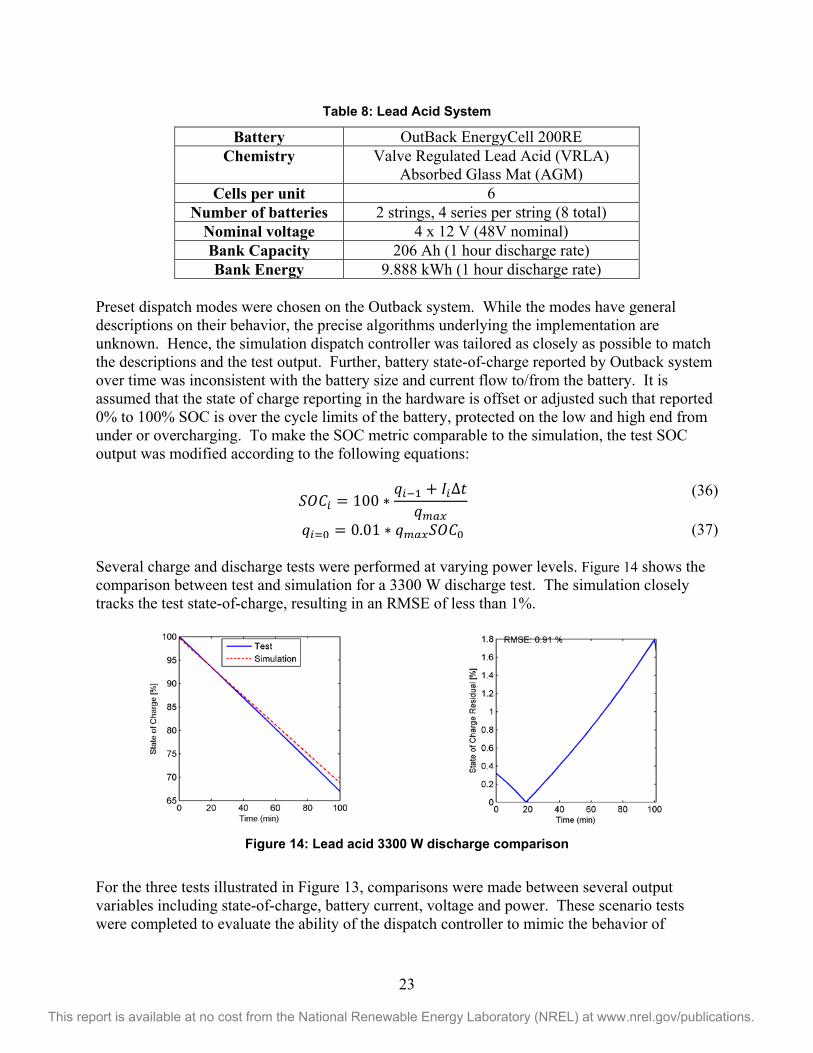
= 0.01 (37) Several charge and discharge tests were performed at varying power levels. Figure 14 shows the comparison between test and simulation for a 3300 W discharge test. The simulation closely tracks the test state-of-charge, resulting in an RMSE of less than 1%.

Figure 14: Lead acid 3300 W discharge comparison

For the three tests illustrated in Figure 13, comparisons were made between several output variables including state-of-charge, battery current, voltage and power. These scenario tests were completed to evaluate the ability of the dispatch controller to mimic the behavior of

24


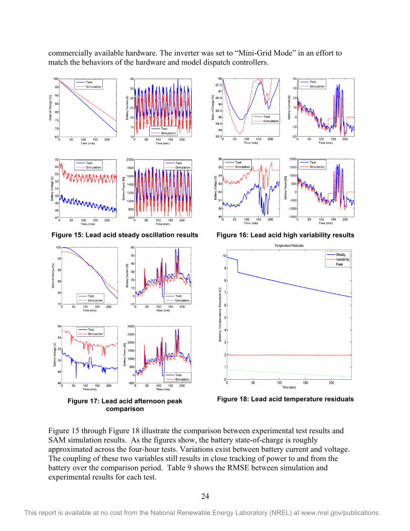
commercially available hardware. The inverter was set to “Mini-Grid Mode” in an effort to match the behaviors of the hardware and model dispatch controllers.

Figure 15: Lead acid steady oscillation results

Figure 16: Lead acid high variability results

Figure 17: Lead acid afternoon peak

comparison

Figure 18: Lead acid temperature residuals

Figure 15 through Figure 18 illustrate the comparison between experimental test results and SAM simulation results. As the figures show, the battery state-of-charge is roughly approximated across the four-hour tests. Variations exist between battery current and voltage. The coupling of these two variables still results in close tracking of power to and from the battery over the comparison period. Table 9 shows the RMSE between simulation and experimental results for each test.

25


Table 9: Root Mean Square Errors

State of Charge (%)

Current (A)

Voltage (V)

Power (W)

Temperature ( C)

Steady 3.76 6.12 3.78 249.86 7.85 Variability 0.82 7.74 2.65 397.53 1.97 Afternoon 1.47 7.05 3.76 325.36 0.52

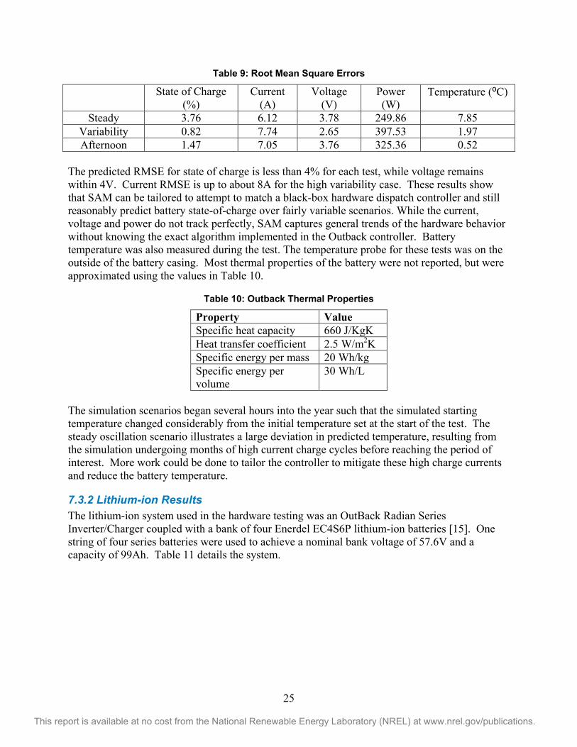
The predicted RMSE for state of charge is less than 4% for each test, while voltage remains within 4V. Current RMSE is up to about 8A for the high variability case. These results show that SAM can be tailored to attempt to match a black-box hardware dispatch controller and still reasonably predict battery state-of-charge over fairly variable scenarios. While the current, voltage and power do not track perfectly, SAM captures general trends of the hardware behavior without knowing the exact algorithm implemented in the Outback controller. Battery temperature was also measured during the test. The temperature probe for these tests was on the outside of the battery casing. Most thermal properties of the battery were not reported, but were approximated using the values in Table 10.

Table 10: Outback Thermal Properties

Property Value Specific heat capacity 660 J/KgK Heat transfer coefficient 2.5 W/m2K Specific energy per mass 20 Wh/kg Specific energy per volume

30 Wh/L

The simulation scenarios began several hours into the year such that the simulated starting temperature changed considerably from the initial temperature set at the start of the test. The steady oscillation scenario illustrates a large deviation in predicted temperature, resulting from the simulation undergoing months of high current charge cycles before reaching the period of interest. More work could be done to tailor the controller to mitigate these high charge currents and reduce the battery temperature.

7.3.2 Lithium-ion Results The lithium-ion system used in the hardware testing was an OutBack Radian Series Inverter/Charger coupled with a bank of four Enerdel EC4S6P lithium-ion batteries [15]. One string of four series batteries were used to achieve a nominal bank voltage of 57.6V and a capacity of 99Ah. Table 11 details the system.

26


Table 11: Lithium-ion System

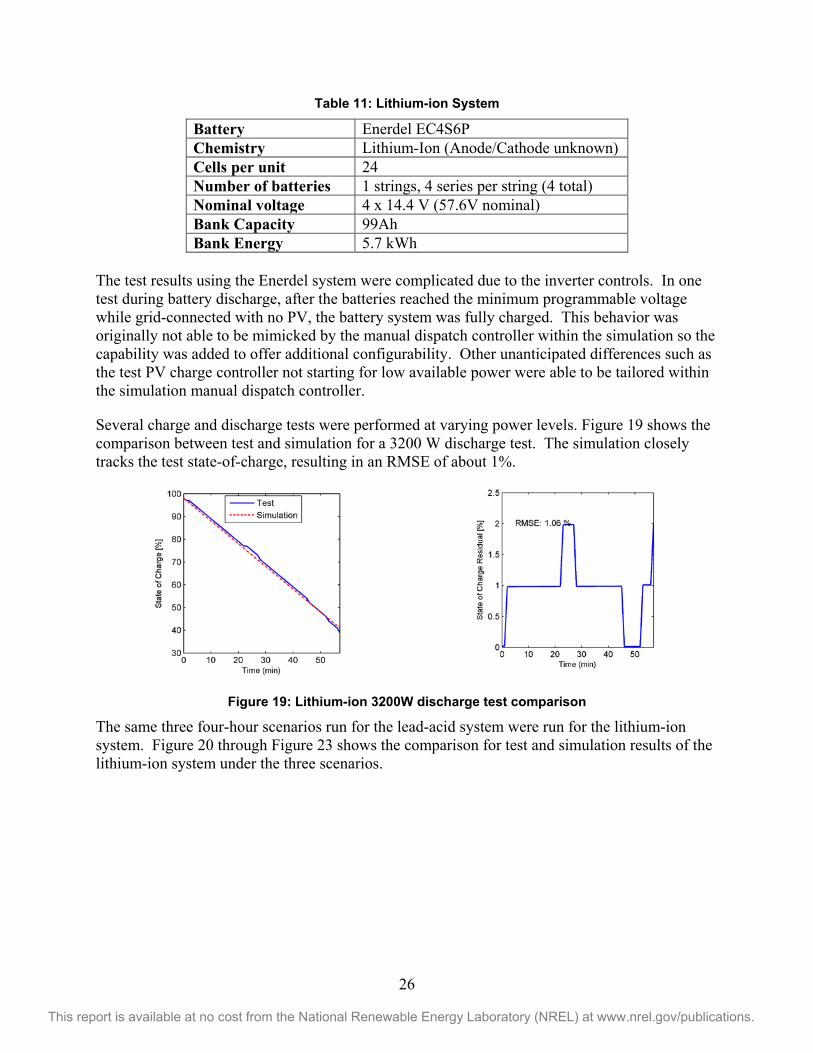
Battery Enerdel EC4S6P Chemistry Lithium-Ion (Anode/Cathode unknown) Cells per unit 24 Number of batteries 1 strings, 4 series per string (4 total) Nominal voltage 4 x 14.4 V (57.6V nominal) Bank Capacity 99Ah Bank Energy 5.7 kWh

The test results using the Enerdel system were complicated due to the inverter controls. In one test during battery discharge, after the batteries reached the minimum programmable voltage while grid-connected with no PV, the battery system was fully charged. This behavior was originally not able to be mimicked by the manual dispatch controller within the simulation so the capability was added to offer additional configurability. Other unanticipated differences such as the test PV charge controller not starting for low available power were able to be tailored within the simulation manual dispatch controller.

Several charge and discharge tests were performed at varying power levels. Figure 19 shows the comparison between test and simulation for a 3200 W discharge test. The simulation closely tracks the test state-of-charge, resulting in an RMSE of about 1%.

Figure 19: Lithium-ion 3200W discharge test comparison

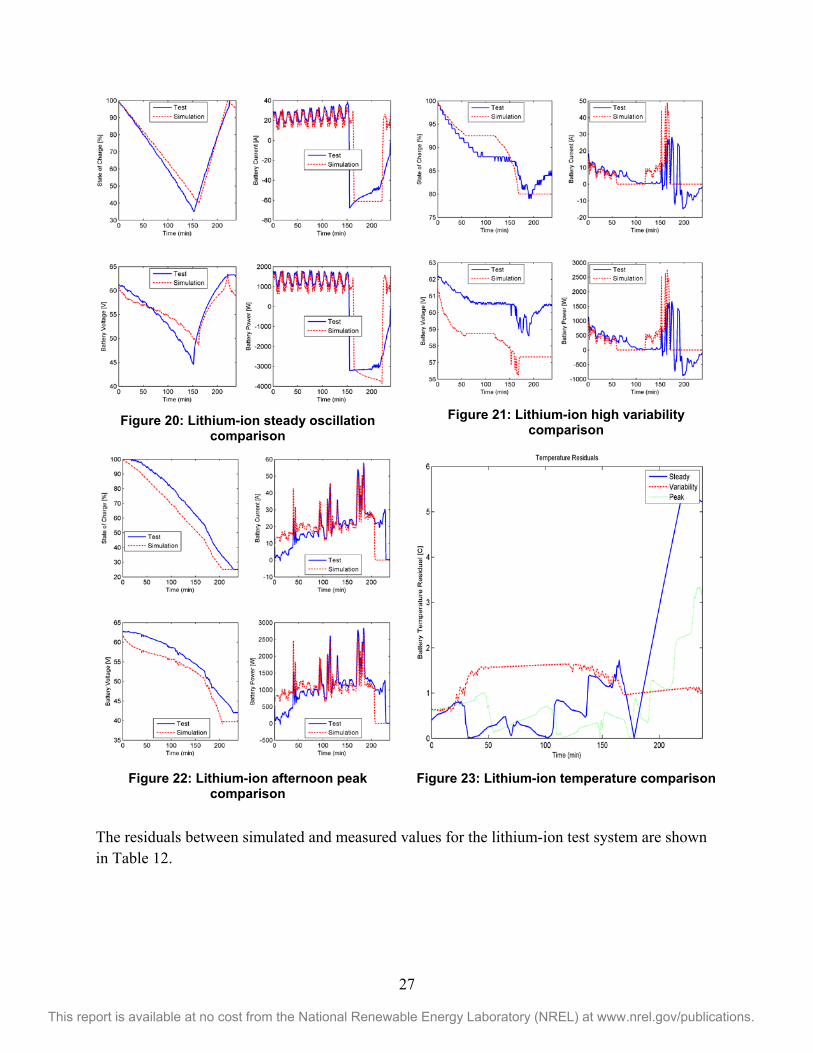
The same three four-hour scenarios run for the lead-acid system were run for the lithium-ion system. Figure 20 through Figure 23 shows the comparison for test and simulation results of the lithium-ion system under the three scenarios.

27


Figure 20: Lithium-ion steady oscillation

comparison

Figure 21: Lithium-ion high variability

comparison

Figure 22: Lithium-ion afternoon peak

comparison

Figure 23: Lithium-ion temperature comparison

The residuals between simulated and measured values for the lithium-ion test system are shown in Table 12.

28


Table 12: Lithium-ion Residuals

State of Charge (%)

Current (A) Voltage (V)

Power (W)

Temperature ( C)

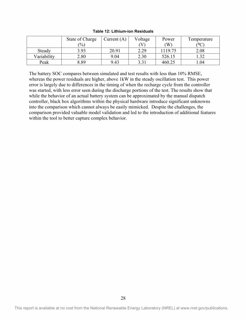
Steady 3.93 20.91 2.29 1119.75 2.08 Variability 2.80 9.04 2.30 526.15 1.32

Peak 8.89 9.43 3.31 460.25 1.04 The battery SOC compares between simulated and test results with less than 10% RMSE, whereas the power residuals are higher, above 1kW in the steady oscillation test. This power error is largely due to differences in the timing of when the recharge cycle from the controller was started, with less error seen during the discharge portions of the test. The results show that while the behavior of an actual battery system can be approximated by the manual dispatch controller, black box algorithms within the physical hardware introduce significant unknowns into the comparison which cannot always be easily mimicked. Despite the challenges, the comparison provided valuable model validation and led to the introduction of additional features within the tool to better capture complex behavior.

29


8 Conclusion A generic battery model has been added to the free, publically available System Advisor Model, which allows users to consider lead-acid or lithium-ion batteries added to PV system. The model predicts detailed parameters such as battery state-of-charge, terminal voltage, and capacity fade due to cycling and temperature. A new lifetime simulation mode allows a user to run a simulation over the entire analysis period to predict variable capital costs associated with battery bank replacements. Validations of the model against commercially available software packages showed key metrics within 5%. Comparisons against data obtained from controlled hardware testing with multiple commercially available battery systems showed the SAM model was able to predict battery state of charge within 9% RMSE over six four-hour tests across lead-acid and lithium-ion systems. This powerful new feature of SAM will enable further investigation into the important topic of the economic performance of PV coupled with battery storage.

30


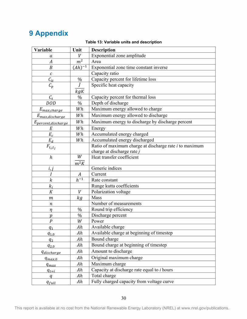
9 Appendix Table 13: Variable units and description

Variable Unit Description Exponential zone amplitude Area ( ) Exponential zone time constant inverse Capacity ratio % Capacity percent for lifetime loss Specific heat capacity

% Capacity percent for thermal loss % Depth of discharge

, Maximum energy allowed to charge , Maximum energy allowed to discharge

, Maximum energy to discharge by discharge percent Energy Accumulated energy charged Accumulated energy discharged

, Ratio of maximum charge at discharge rate i to maximum charge at discharge rate j

Heat transfer coefficient

, Generic indices Current Rate constant Runge kutta coefficients Polarization voltage Mass Number of measurements % Round trip efficiency % Discharge percent Power Available charge

, Available charge at beginning of timestep Bound charge

, Bound charge at beginning of timestep Amount to discharge

, Original maximum charge Maximum charge Capacity at discharge rate equal to i hours

Total charge Fully charged capacity from voltage curve

31


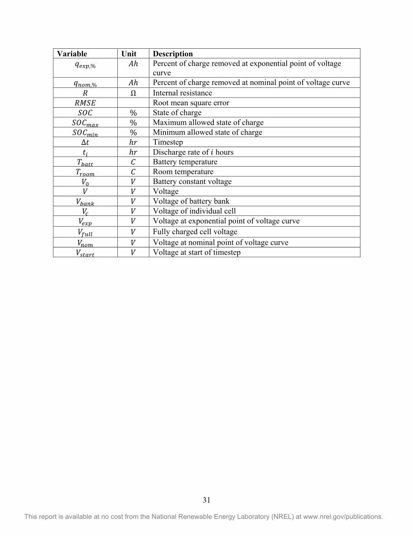
Variable Unit Description ,% Percent of charge removed at exponential point of voltage

curve ,% Percent of charge removed at nominal point of voltage curve

Internal resistance Root mean square error

% State of charge % Maximum allowed state of charge % Minimum allowed state of charge

Timestep Discharge rate of hours

Battery temperature Room temperature

Battery constant voltage Voltage

Voltage of battery bank Voltage of individual cell Voltage at exponential point of voltage curve Fully charged cell voltage Voltage at nominal point of voltage curve Voltage at start of timestep

32


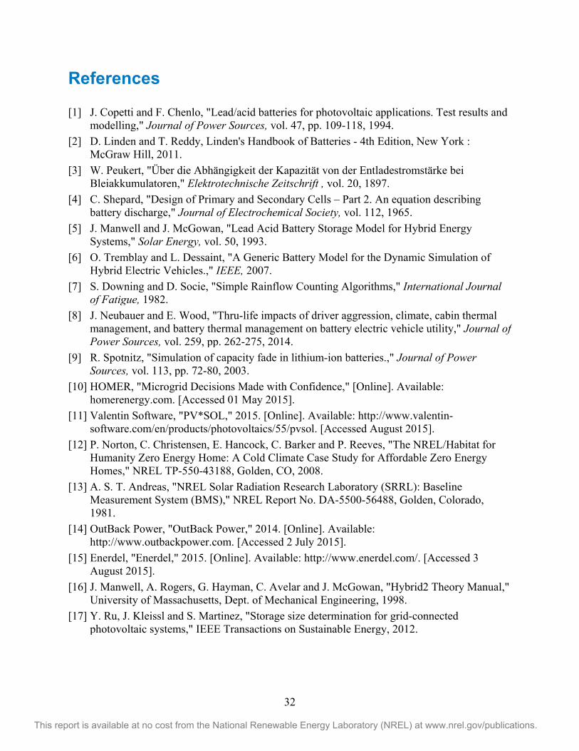
References [1] J. Copetti and F. Chenlo, "Lead/acid batteries for photovoltaic applications. Test results and

modelling," Journal of Power Sources, vol. 47, pp. 109-118, 1994. [2] D. Linden and T. Reddy, Linden's Handbook of Batteries - 4th Edition, New York :

McGraw Hill, 2011. [3] W. Peukert, "Über die Abhängigkeit der Kapazität von der Entladestromstärke bei

Bleiakkumulatoren," Elektrotechnische Zeitschrift , vol. 20, 1897. [4] C. Shepard, "Design of Primary and Secondary Cells – Part 2. An equation describing

battery discharge," Journal of Electrochemical Society, vol. 112, 1965. [5] J. Manwell and J. McGowan, "Lead Acid Battery Storage Model for Hybrid Energy

Systems," Solar Energy, vol. 50, 1993. [6] O. Tremblay and L. Dessaint, "A Generic Battery Model for the Dynamic Simulation of

Hybrid Electric Vehicles.," IEEE, 2007. [7] S. Downing and D. Socie, "Simple Rainflow Counting Algorithms," International Journal

of Fatigue, 1982. [8] J. Neubauer and E. Wood, "Thru-life impacts of driver aggression, climate, cabin thermal

management, and battery thermal management on battery electric vehicle utility," Journal of Power Sources, vol. 259, pp. 262-275, 2014.

[9] R. Spotnitz, "Simulation of capacity fade in lithium-ion batteries.," Journal of Power Sources, vol. 113, pp. 72-80, 2003.

[10] HOMER, "Microgrid Decisions Made with Confidence," [Online]. Available: homerenergy.com. [Accessed 01 May 2015].

[11] Valentin Software, "PV*SOL," 2015. [Online]. Available: http://www.valentin-software.com/en/products/photovoltaics/55/pvsol. [Accessed August 2015].

[12] P. Norton, C. Christensen, E. Hancock, C. Barker and P. Reeves, "The NREL/Habitat for Humanity Zero Energy Home: A Cold Climate Case Study for Affordable Zero Energy Homes," NREL TP-550-43188, Golden, CO, 2008.

[13] A. S. T. Andreas, "NREL Solar Radiation Research Laboratory (SRRL): Baseline Measurement System (BMS)," NREL Report No. DA-5500-56488, Golden, Colorado, 1981.

[14] OutBack Power, "OutBack Power," 2014. [Online]. Available: http://www.outbackpower.com. [Accessed 2 July 2015].

[15] Enerdel, "Enerdel," 2015. [Online]. Available: http://www.enerdel.com/. [Accessed 3 August 2015].

[16] J. Manwell, A. Rogers, G. Hayman, C. Avelar and J. McGowan, "Hybrid2 Theory Manual," University of Massachusetts, Dept. of Mechanical Engineering, 1998.

[17] Y. Ru, J. Kleissl and S. Martinez, "Storage size determination for grid-connected photovoltaic systems," IEEE Transactions on Sustainable Energy, 2012.

Documents

Technoeconomic Modeling of Battery Energy … lead-acid and lithium-ion battery models have been integrated with photovoltaic models giving System Advisor Model (SAM) the ability to