Ten things you should know about quadrature

Nick Trefethen, Vanderbilt, Wed. 28 May 2014 @ 8:35 PM

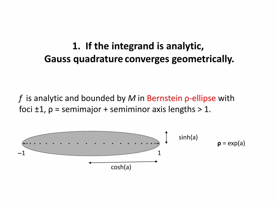
f is analytic and bounded by M in Bernstein ρ-ellipse with foci ±1, ρ = semimajor + semiminor axis lengths > 1.

cosh(a)

sinh(a)

1 1

ρ = exp(a)

1. If the integrand is analytic, Gauss quadrature converges geometrically.

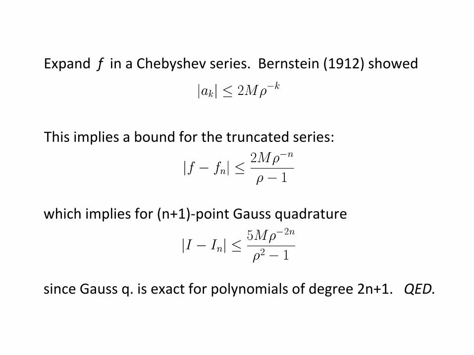
Expand f in a Chebyshev series. Bernstein (1912) showed

This implies a bound for the truncated series:

which implies for (n+1)-point Gauss quadrature

since Gauss q. is exact for polynomials of degree 2n+1. QED.

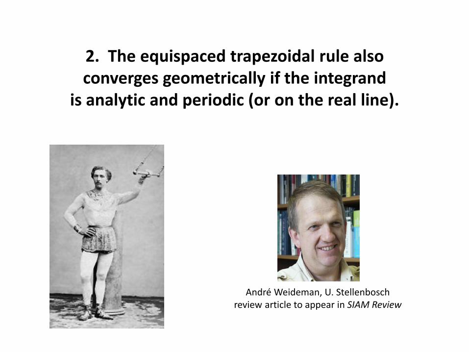
2. The equispaced trapezoidal rule also converges geometrically if the integrand

is analytic and periodic (or on the real line).

André Weideman, U. Stellenbosch review article to appear in SIAM Review

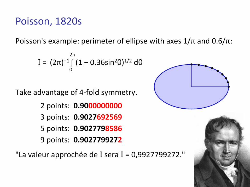
Poisson, 1820s

0

2π

Poisson's example: perimeter of ellipse with axes 1/π and 0.6/π:

I = (2π)−1 ∫ (1 − 0.36sin2θ)1/2 dθ Take advantage of 4-fold symmetry.

2 points: 0.9000000000

3 points: 0.9027692569

5 points: 0.9027798586

9 points: 0.9027799272

"La valeur approchée de I sera I = 0,9927799272."

2/20

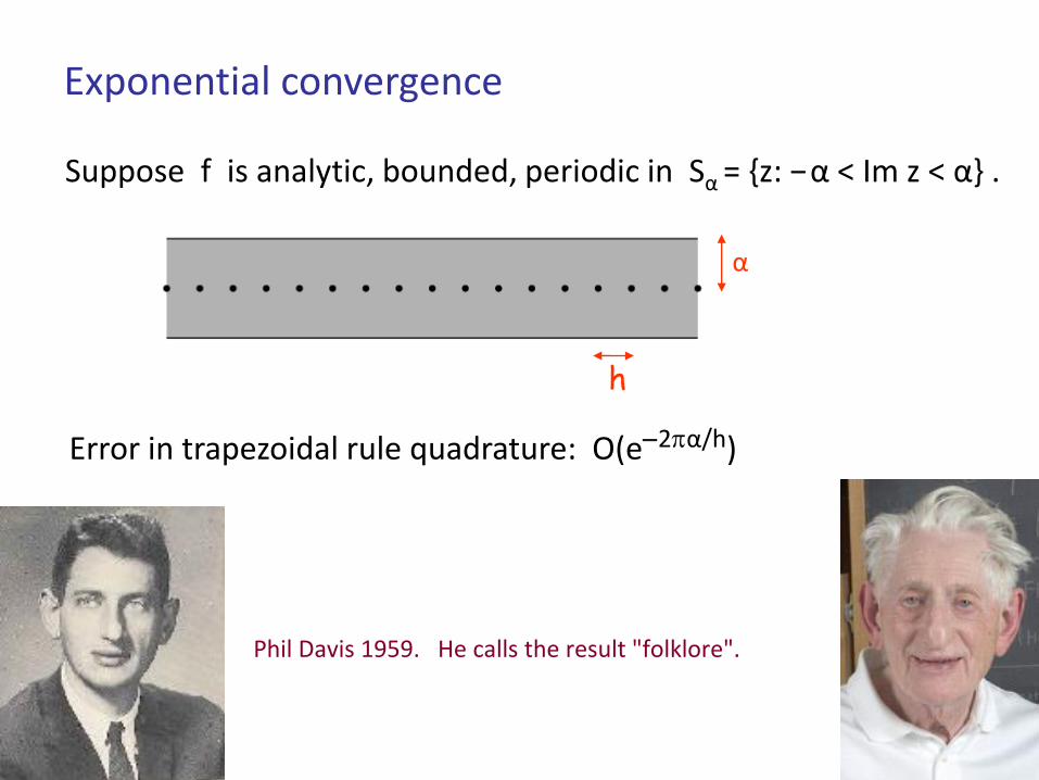
Suppose f is analytic, bounded, periodic in Sα = {z: −α < Im z < α} .

h

α

Exponential convergence

Phil Davis 1959. He calls the result "folklore".

Error in trapezoidal rule quadrature: O(e2α/h)

3/20

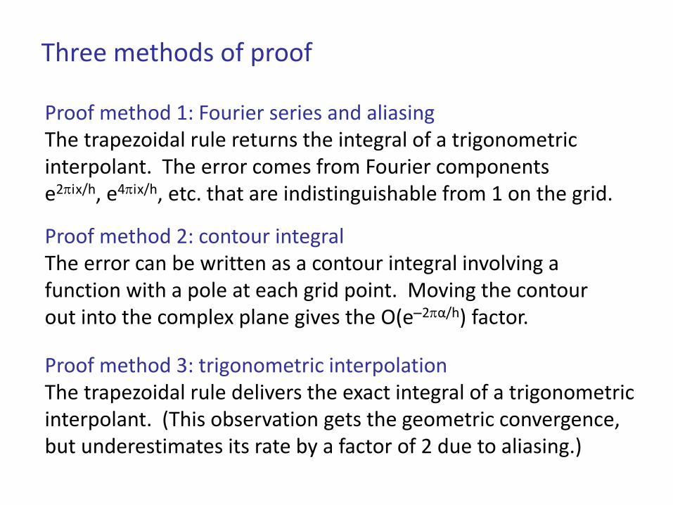
Three methods of proof

Proof method 1: Fourier series and aliasing The trapezoidal rule returns the integral of a trigonometric interpolant. The error comes from Fourier components e2ix/h, e4ix/h, etc. that are indistinguishable from 1 on the grid.

Proof method 2: contour integral The error can be written as a contour integral involving a function with a pole at each grid point. Moving the contour out into the complex plane gives the O(e2α/h) factor.

Proof method 3: trigonometric interpolation The trapezoidal rule delivers the exact integral of a trigonometric interpolant. (This observation gets the geometric convergence, but underestimates its rate by a factor of 2 due to aliasing.)

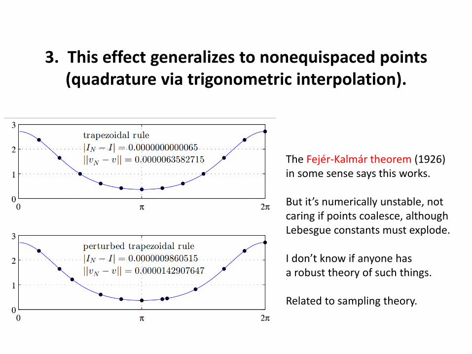
3. This effect generalizes to nonequispaced points (quadrature via trigonometric interpolation).

The Fejér-Kalmár theorem (1926) in some sense says this works. But it’s numerically unstable, not caring if points coalesce, although Lebesgue constants must explode. I don’t know if anyone has a robust theory of such things. Related to sampling theory.

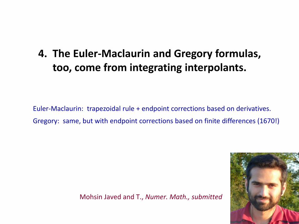
4. The Euler-Maclaurin and Gregory formulas, too, come from integrating interpolants.

Mohsin Javed and T., Numer. Math., submitted

Euler-Maclaurin: trapezoidal rule + endpoint corrections based on derivatives.

Gregory: same, but with endpoint corrections based on finite differences (1670!)

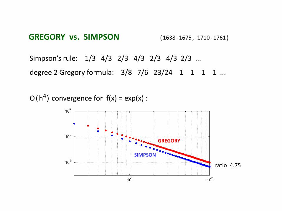
GREGORY vs. SIMPSON

Simpson’s rule: 1/3 4/3 2/3 4/3 2/3 4/3 2/3 ...

degree 2 Gregory formula: 3/8 7/6 23/24 1 1 1 1 ...

O(h4) convergence for f(x) = exp(x) :

SIMPSON

GREGORY

ratio 4.75

( 1638 - 1675 , 1710 - 1761 )

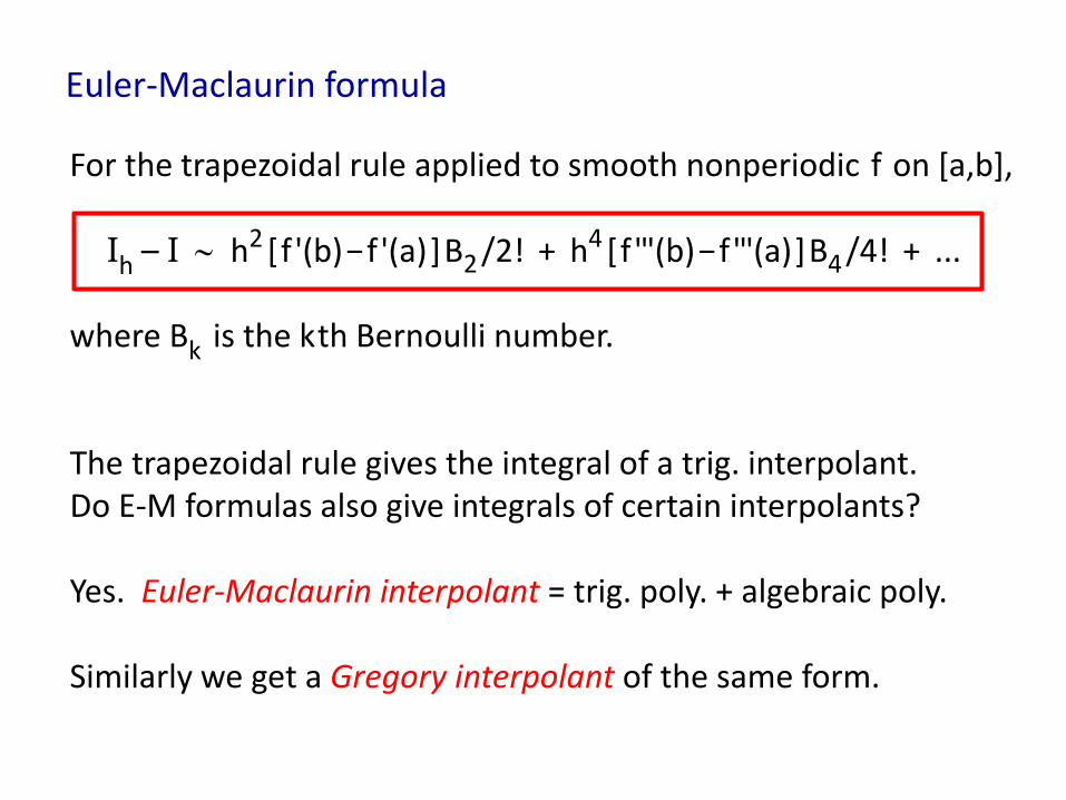
Euler-Maclaurin formula

For the trapezoidal rule applied to smooth nonperiodic f on [a,b], Ih – I h2 [f '(b)−f '(a)]B2 /2! + h4 [f '''(b)−f '''(a)]B4 /4! + ... where Bk is the kth Bernoulli number.

The trapezoidal rule gives the integral of a trig. interpolant. Do E-M formulas also give integrals of certain interpolants? Yes. Euler-Maclaurin interpolant = trig. poly. + algebraic poly. Similarly we get a Gregory interpolant of the same form.

5. Gauss nodes and weights can be computed in O(n) time.

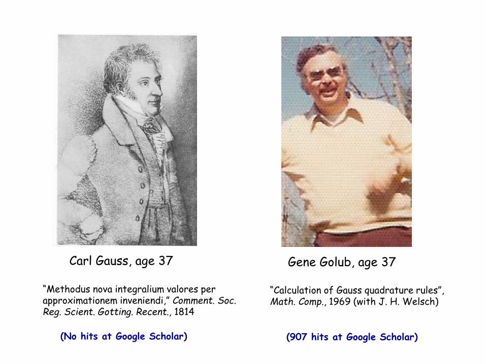
Gene Golub, age 37

“Calculation of Gauss quadrature rules”, Math. Comp., 1969 (with J. H. Welsch)

Carl Gauss, age 37

“Methodus nova integralium valores per approximationem inveniendi,” Comment. Soc. Reg. Scient. Gotting. Recent., 1814

(907 hits at Google Scholar) (No hits at Google Scholar)

Nodes and weights in O(n) time

Nick Hale, Oxford → Stellenbosch Alex Townsend, Oxford → MIT

Glaser, Liu + Rokhlin 2007 Bogaert, Michiels + Fostier 2012 Hale + Townsend 2013 all in SIAM J Sci Comp

[s,w] = legpts(n)

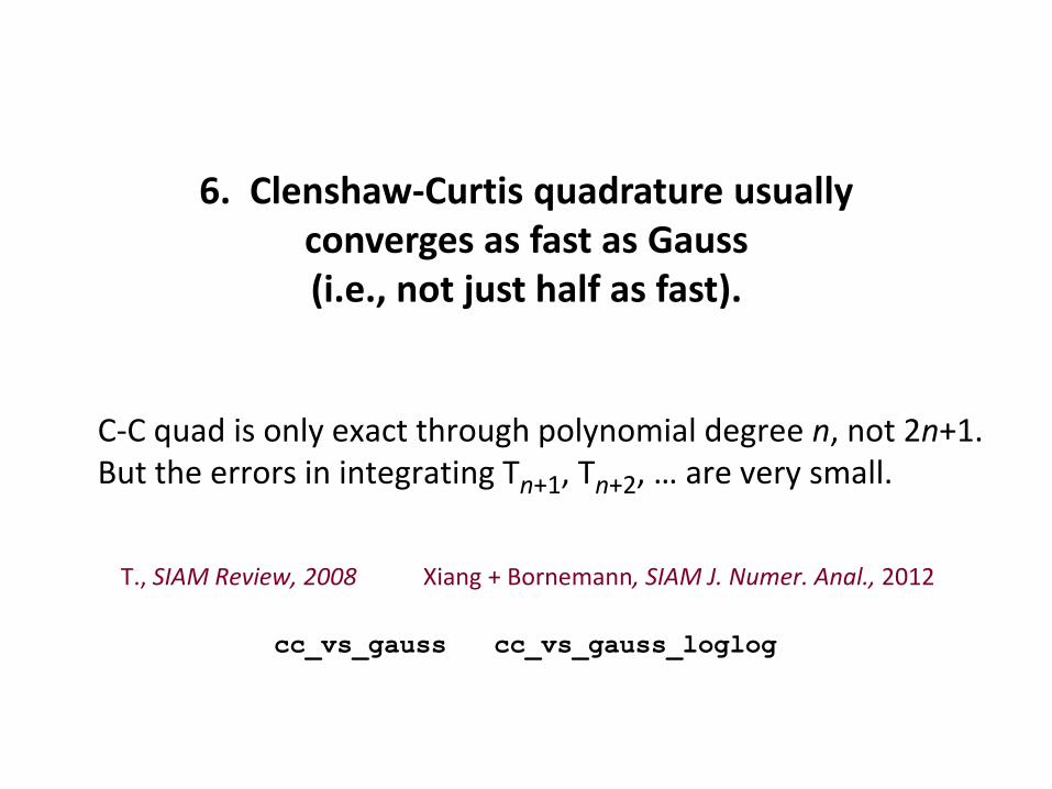
6. Clenshaw-Curtis quadrature usually converges as fast as Gauss (i.e., not just half as fast).

cc_vs_gauss cc_vs_gauss_loglog

T., SIAM Review, 2008 Xiang + Bornemann, SIAM J. Numer. Anal., 2012

C-C quad is only exact through polynomial degree n, not 2n+1. But the errors in integrating Tn+1, Tn+2, … are very small.

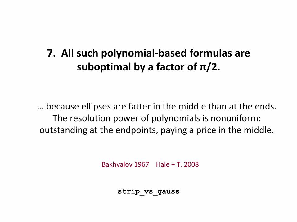
7. All such polynomial-based formulas are suboptimal by a factor of π/2.

strip_vs_gauss

Bakhvalov 1967 Hale + T. 2008

… because ellipses are fatter in the middle than at the ends. The resolution power of polynomials is nonuniform:

outstanding at the endpoints, paying a price in the middle.

8. Bending around the negative real axis evaluates inverse Laplace transforms and

special functions.

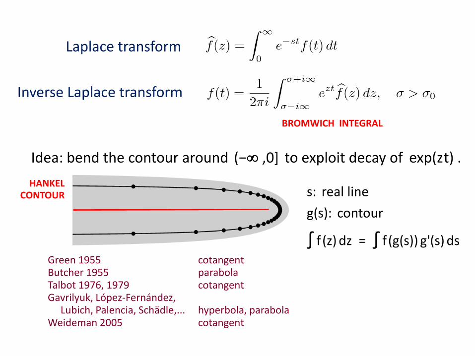
Laplace transform

Inverse Laplace transform

BROMWICH INTEGRAL

Idea: bend the contour around (− ,0] to exploit decay of exp(zt) .

HANKEL CONTOUR

Green 1955 cotangent Butcher 1955 parabola Talbot 1976, 1979 cotangent Gavrilyuk, López-Fernández, Lubich, Palencia, Schädle,... hyperbola, parabola Weideman 2005 cotangent

s: real line

g(s): contour

∫ f (z) dz = ∫ f (g(s)) g'(s) ds

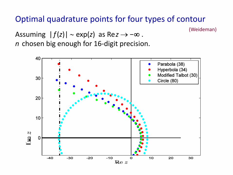
Optimal quadrature points for four types of contour

Assuming | f (z)| exp(z) as Rez − . n chosen big enough for 16-digit precision.

(Weideman)

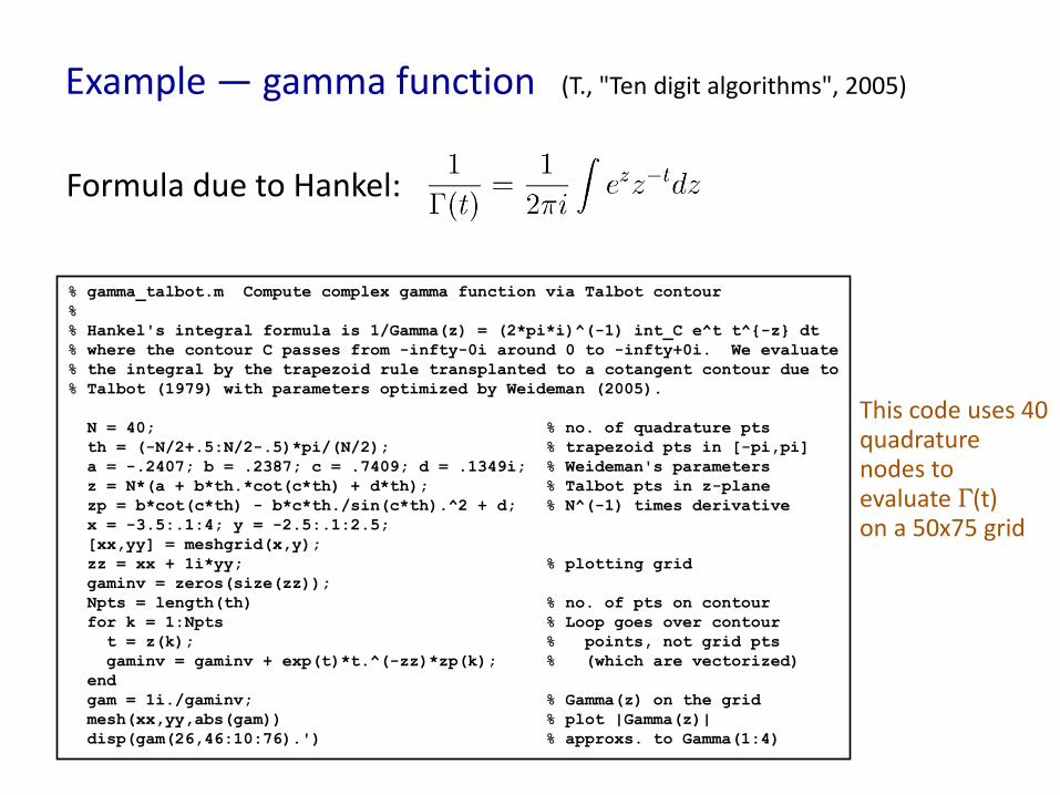
Example — gamma function (T., "Ten digit algorithms", 2005)

% gamma_talbot.m Compute complex gamma function via Talbot contour

%

% Hankel's integral formula is 1/Gamma(z) = (2*pi*i)^(-1) int_C e^t t^{-z} dt

% where the contour C passes from -infty-0i around 0 to -infty+0i. We evaluate

% the integral by the trapezoid rule transplanted to a cotangent contour due to

% Talbot (1979) with parameters optimized by Weideman (2005).

N = 40; % no. of quadrature pts

th = (-N/2+.5:N/2-.5)*pi/(N/2); % trapezoid pts in [-pi,pi]

a = -.2407; b = .2387; c = .7409; d = .1349i; % Weideman's parameters

z = N*(a + b*th.*cot(c*th) + d*th); % Talbot pts in z-plane

zp = b*cot(c*th) - b*c*th./sin(c*th).^2 + d; % N^(-1) times derivative

x = -3.5:.1:4; y = -2.5:.1:2.5;

[xx,yy] = meshgrid(x,y);

zz = xx + 1i*yy; % plotting grid

gaminv = zeros(size(zz));

Npts = length(th) % no. of pts on contour

for k = 1:Npts % Loop goes over contour

t = z(k); % points, not grid pts

gaminv = gaminv + exp(t)*t.^(-zz)*zp(k); % (which are vectorized)

end

gam = 1i./gaminv; % Gamma(z) on the grid

mesh(xx,yy,abs(gam)) % plot |Gamma(z)|

disp(gam(26,46:10:76).') % approxs. to Gamma(1:4)

Formula due to Hankel:

This code uses 40 quadrature nodes to evaluate Γ(t) on a 50x75 grid

9. Taking the integrand to be a matrix or operator gives methods for computing f (A).

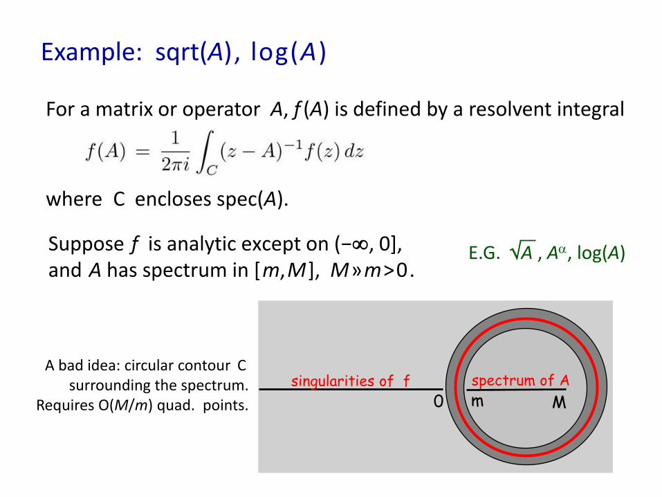
Example: sqrt(A), log(A)

where C encloses spec(A).

For a matrix or operator A, f (A) is defined by a resolvent integral

Suppose f is analytic except on (−, 0], and A has spectrum in [m,M], M»m>0.

E.G. A , A, log(A)

0 singularities of f spectrum of A

m M

A bad idea: circular contour C surrounding the spectrum.

Requires O(M/m) quad. points.

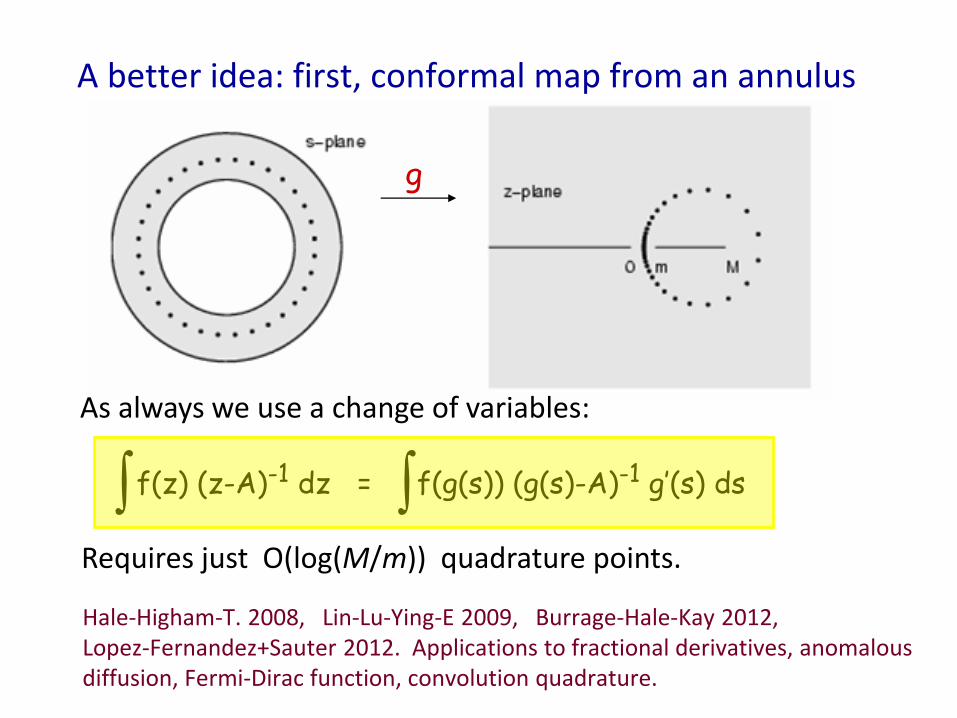
A better idea: first, conformal map from an annulus

g

f(z) (z-A)-1 dz = f(g(s)) (g(s)-A)-1 g’(s) ds

As always we use a change of variables:

Requires just O(log(M/m)) quadrature points.

Hale-Higham-T. 2008, Lin-Lu-Ying-E 2009, Burrage-Hale-Kay 2012, Lopez-Fernandez+Sauter 2012. Applications to fractional derivatives, anomalous diffusion, Fermi-Dirac function, convolution quadrature.

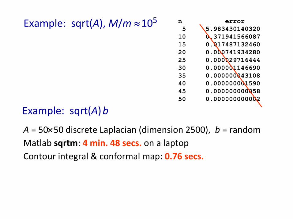
n error

5 5.983430140320

10 0.371941566087

15 0.017487132460

20 0.000741934280

25 0.000029716444

30 0.000001146690

35 0.000000043108

40 0.000000001590

45 0.000000000058

50 0.000000000002

Example: sqrt(A), M/m 105

Example: sqrt(A)b

A = 5050 discrete Laplacian (dimension 2500), b = random

Matlab sqrtm: 4 min. 48 secs. on a laptop

Contour integral & conformal map: 0.76 secs.

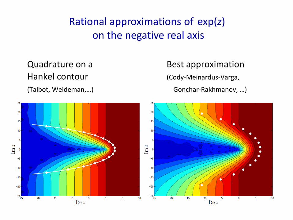
10. Every quadrature formula is a rational or meromorphic approximation.

We use the approximations to estimate accuracy of quadrature formulas for analytic integrands. Conversely, we can use the quadrature formulas to generate approximations.

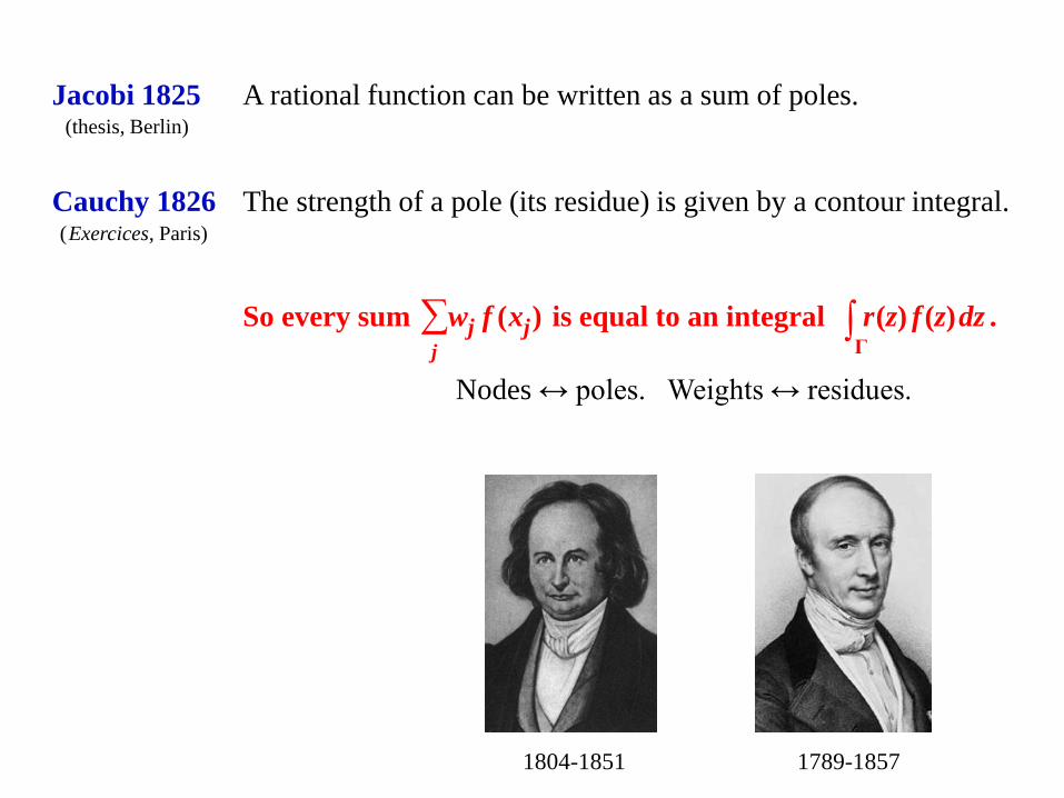
Jacobi 1825 A rational function can be written as a sum of poles.

Cauchy 1826 The strength of a pole (its residue) is given by a contour integral.

So every sum ∑wj f (xj) is equal to an integral r(z) f (z)dz .

Nodes ↔ poles. Weights ↔ residues.

j ∫ Γ

(Exercices, Paris)

(thesis, Berlin)

1804-1851 1789-1857

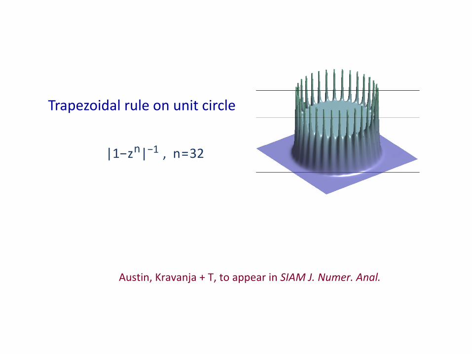
|1−zn|−1 , n=32

Trapezoidal rule on unit circle

Austin, Kravanja + T, to appear in SIAM J. Numer. Anal.

Quadrature on a Hankel contour

(Talbot, Weideman,…)

Rational approximations of exp(z) on the negative real axis

Best approximation (Cody-Meinardus-Varga,

Gonchar-Rakhmanov, …)