Testing Alternative Ground Water Models Using Cross-Validation and Other Methods

Testing Alternative Ground Water ModelsUsing Cross-Validation and Other Methodsby L. Foglia1, S.W. Mehl2, M.C. Hill2, P. Perona3, and P. Burlando3

AbstractMany methods can be used to test alternative ground water models. Of concern in this work are methods able

to (1) rank alternative models (also called model discrimination) and (2) identify observations important to param-eter estimates and predictions (equivalent to the purpose served by some types of sensitivity analysis). Some ofthe measures investigated are computationally efficient; others are computationally demanding. The latter are gen-erally needed to account for model nonlinearity. The efficient model discrimination methods investigated includethe information criteria: the corrected Akaike information criterion, Bayesian information criterion, and general-ized cross-validation. The efficient sensitivity analysis measures used are dimensionless scaled sensitivity (DSS),composite scaled sensitivity, and parameter correlation coefficient (PCC); the other statistics are DFBETAS,Cook’s D, and observation-prediction statistic. Acronyms are explained in the introduction. Cross-validation (CV)is a computationally intensive nonlinear method that is used for both model discrimination and sensitivity analy-sis. The methods are tested using up to five alternative parsimoniously constructed models of the ground watersystem of the Maggia Valley in southern Switzerland. The alternative models differ in their representation ofhydraulic conductivity. A new method for graphically representing CV and sensitivity analysis results for complexmodels is presented and used to evaluate the utility of the efficient statistics. The results indicate that for modelselection, the information criteria produce similar results at much smaller computational cost than CV. For identi-fying important observations, the only obviously inferior linear measure is DSS; the poor performance was ex-pected because DSS does not include the effects of parameter correlation and PCC reveals large parametercorrelations.

IntroductionAn important goal of most models is to provide real-

istic predictions over a range of real space-time condi-tions. Ground water models usually deal with a smallamount of uncertain data and potentially many parame-ters for which values need to be determined. Values mea-sured at the laboratory scale or even the small field scale

generally do not directly apply to a regional scale model(Brooks et al. 1994). This commonly results in groundwater models being calibrated and often leads to thedevelopment of many candidate models that can differ inthe processes included, representation of boundary condi-tion, distribution of system characteristics, and parametervalues. Given a set of candidate models, statistical techni-ques often are used to discriminate between and evaluatevarious aspects of the different models.

There have been substantial efforts to developmodel discrimination statistics (Akaike 1974; Carrera andNeumann 1986; Burnham and Anderson 2002), cross-validation (CV) methods (Efron 1982), and sensitivityanalysis methods (Saltelli et al. 2000). In this work,model discrimination is pursued using information crite-ria: the corrected Akaike information criterion (AICc),Bayesian information criterion (BIC), and generalizedcross-validation (GCV), and using CV (e.g., Jackknife,

1Corresponding author: IfU, ETH Zurich, Switzerland.Current address: University of California, Davis, Department of

Civil and Environmental Engineering, One Shields Ave., Davis, CA95616; (530) 752-0586; fax (530) 752-7872; [email protected]

2Ifu, ETH, Zurich, Switzerland.3U.S. Geological Survey, Boulder, CO 80301.Received January 2006, accepted March 2007.Copyright ª 2007 The Author(s)Journal compilationª 2007 National GroundWater AssociationNo claim to original US government works.doi: 10.1111/j.1745-6584.2007.00341.x

Vol. 45, No. 5—GROUND WATER—September–October 2007 (pages 627–641) 627

Bootstrapping; see, for instance, Efron 1982; Wu 1986;Good 2001). Sensitivity analysis is conducted using CVand the linear statistical measures dimensionless scaledsensitivity (DSS), composite scaled sensitivity (CSS),parameter correlation coefficient (PCC), observation-pre-diction (OPR) statistic, Cook’s D, and DFBETAS. Whileother methods and statistics exist, the group studied inthis work includes a set that is often used.

Model discrimination has long been studied, but theformulation of a general rule to evaluate the differentmodels is still difficult to identify (Akaike 1974; Efron1982; Burnham and Anderson 2002, 2004; Poeter andAnderson 2005). In this work, we analyze the model dis-crimination and selection techniques in the context ofalternative models implemented for the ground water sys-tem of Maggia Valley in southern Switzerland.

A novelty of this work is the use of CV for modelselection and identification of the observations used inthe context of ground water models. CV requires applica-tions with short computational time, for example, thetime series analysis of Regonda et al. (2005) and the krig-ing analysis of Isaaks and Srivastava (1989). Because ofthe computational requirements, the use of CV for groundwater models has been limited. Christensen and Cooley(1999) used CV to compare linear and nonlinear pre-diction intervals but not the purposes addressed in thiswork. To our knowledge, the present work is one of thefirst uses of CV for model selection and identification ofimportant observations in a practical ground water model.In addition, this work presents a new graphical method ofportraying CV results. Though developed independently,the graphical method has some similarity to a techniquepresented by Perona et al. (2000).

The principal purpose of this paper is to addressthree questions: (1) How does CV compare to informa-tion criteria for model discrimination, given nonlinearmodels? (2) When identifying important observations ofnonlinear models, how well do statistics based on lineartheory perform compared to CV? and (3) Can we use CVto evaluate the dependence of model fit on each observa-tion? The insights gained from answering these questionscan be used to guide application of the computationallyefficient methods to the vast majority of ground watermodels for which computational times make CV imprac-tical. The model we are using is well suited for the statis-tical experiments needed to address these questionsbecause its degree of nonlinearity is similar to many con-structed ground water models. While other ground watermodels may include other or additional system compo-nents such as areal recharge, springs, evapotranspiration,or transport, the results of this work hopefully provideinsight into other models that have a similar degree ofnonlinearity. For less nonlinear models, it is expected thatthe linear statistics would perform better than the resultsof this work suggest; for more nonlinear models, it is ex-pected that they would perform worse.

These questions are addressed using five nonlinear,fast, and stable ground water/surface water models of theMaggia Valley in southern Switzerland. The groundwater/surface water model was constructed using MOD-FLOW-2000 and its River Package, and it was developed

parsimoniously to guarantee numerical stability, compu-tational efficiency, and conceptual transparency. In thiswork, we focus on a parameterization of the K field basedon geological and hydrological information. Highlyparameterized methods such as those used by Moore andDoherty (2005) and others were not considered in partbecause the computational requirements make a CV anal-ysis impractical.

This work is organized as follows: first, the methodsused and their role within this work are described, thegeneral features of the ground water model are examined,results are presented in three thematic subsectionstogether with a discussion, and conclusions based onthese results are given.

MethodsIn this section, we present the statistical methods for

model discrimination and evaluation used in this study;some of their basic features are listed in Table 1. Moredetails, including the equations used to calculate theinformation criteria and linear sensitivity analysis statis-tics, are presented in Appendix 1. The equations pre-sented assume a diagonal weight matrix, but extension toa full weight matrix is straightforward (see, e.g., Hill andTiedeman 2007, 27–28, 34–35).

Some of the statistics considered are best classifiedas measures of leverage, and some as measures of influ-ence, as shown in Table 1. Measures of leverage identifyobservations that are sensitive in a way that causes the ob-served value to potentially have a profound effect on theregression results. For a linear model, measures of lever-age depend only on the independent variables associatedwith an observation, such as type, location, and time (Helseland Hirsch 2002, 247). For a nonlinear model, measuresof leverage can change with the parameters values.

Measures of influence reflect the actual effect of anobservation on the regression. Observations with high in-fluence more strongly affect the estimated parameter val-ues than other observations. Observations generally need tohave high leverage to have high influence. An observationwith high leverage tends to have high influence if theobserved value in some way contradicts other observations.Influence is generally considered in linear regression anal-ysis (Cook and Weisberg 1982; Tonkin and Larson 2002)and rarely in nonlinear regression analysis, as it is here.

Observations and predictions are considered in thispaper. There are 32 heads and 6 discharge measurements.In this work, all predictions are coincident with observa-tions. Thus, predictions are used in two ways: (1) as sim-ulated values associated with observations in modelcalibration (these are also called simulated equivalents toobservations) and (2) as simulated values for which asso-ciated measurements are omitted from model calibrationin CV experiments.

Information Criteria: AIC, AICc, BIC, and GCV StatisticsCV is computationally demanding, so it is not ap-

plied to all five models developed for the Maggia Valley.Instead, model complexity as measured by the number ofestimated hydraulic conductivity parameters and model

628 L. Foglia et al. GROUND WATER 45, no. 5: 627–641

probability as determined based on information criteriaare used in this work to identify models to be analyzedusing CV.

We consider three information criteria: AICc, BIC,and GCV; equations are presented in Appendix 1. Theinformation criteria provide a penalty for adding parame-ters that has to be overcome by improved model fit forthe model with the added parameter(s) to be competitive.The information criteria values are computed for eachmodel and smaller criterion values indicate more proba-ble models. Commonly, the criteria values are equallysmall for different models, and multiple models arehighly probable. For the AICc criteria, we also presentmodel weights and inverted evidence ratios, which arepart of the Kullback-Leibler analysis described by Burnhamand Anderson (2002) and Poeter and Hill (2007).

Among the numerous information criteria for modeldiscrimination, we can distinguish two principal groups(Burnham and Anderson 2004; Poeter and Anderson2005): (1) information criteria based on the idea that allmodels only approximate reality, such as AIC and AICc,and (2) information criteria based on the idea that withinour ensemble of models, we can find the ‘‘true’’ model,such as BIC. AIC and BIC are the most widely usedmethods for model selection (Carrera and Neumann1986; Hill 1998; Burnham and Anderson 2002, 2004).Here, we use the second-order information criterion forAIC, which is AICc. AICc performs better than AICwhen the number of parameters increases relative to thesize of the sample (Burnham and Anderson 2002; Poeterand Anderson 2005).

GCV also is used to guide model selection (Regondaet al. 2005). The GCV statistic presented here is an infor-mation criterion similar to AICc and BIC and should notbe confused with the CV, which is applied later in thepaper. GCV estimates the predictive error rather than fit-ting error and therefore predictive error sum of squares isa precursor to GCV (Craven and Whaba 1979). The pen-alty assessed by GCV as parameters are added is similarto that of BIC, as shown in Appendix 1.

Cross-ValidationThe goal of CV is to evaluate the dependence of the

model fit and estimated parameter values on each obser-vation. Such evaluation can be used for model selection(Chernick 1999, 105–106; Burnham and Anderson 2002,36). During the past decade, CV techniques have beenextensively developed in the statistical literature (Shao1993; Chernick 1999; Good 2001).

In our work, we apply CV techniques by omittingone observation (leave-one-out) or a group of observa-tions, and we recalibrate the model using nonlinearregression. The CV technique produces a measure ofinfluence equal to how much the estimated parameter val-ues and the simulated values change when observationsare omitted. Influence measures are generally used toassess the importance of the observations to parametersand simulated values: relative to linear methods that mea-sure leverage, an actual and not potential effect is mea-sured; relative to linear methods that measure influence,the CV results account for all types of nonlinearity. Asalready explained, a major problem with CV is the

Table 1Summary of the Methods Used in This Work

StatisticLeverage

of Influence

Measures effect on

Does itAddressModel

Discrimination?Equation inThis Paper

Parameters(each or all)

CummulativeModel Fit

SimulatedValue orPrediction(each or all)

Information criteria used for model discriminationAICc — — — — Yes 6BIC — — — — Yes 7GCV — — — — Yes 8

Nonlinear measures: statistics from CVParameter influence statistic Influence Each — Each — 1Adjusted SSWR Influence — 3 All Yes 2Simulated value influence statistic Influence — — All Yes 3CV weighted residual Influence — — Each Yes 4CVobjective function Influence — 3 All Yes 5

Linear measuresDSS Leverage Each — Each — 10CSS Leverage Each — All — 11Cook’s D1 Influence All — Each — 12DFBETAS Influence Each — Each — 13Leverage statistics Leverage — — Each — 14OPR Leverage2 Each — Each — 16

Note: —, statistics not applicable.1Linear measure but also valid for large total nonlinearity if intrinsic nonlinearity is small (Yager 1998).2Specifically, OPR measures the effect on prediction standard deviation of omitting or adding one or more observations.

L. Foglia et al. GROUND WATER 45, no. 5: 627–641 629

computational demand. In our work, the forward execu-tion time of the ground water model is just a few secondsand regression runs are only a few minutes, which allowsus to investigate CV.

ProcedureCV is composed of six steps: (1) omit one or more

observations; (2) use the new observation set to estimatea new set of parameter values using nonlinear regression;(3) calculate simulated equivalents to all of the observa-tions using the new parameter values; (4) calculate statis-tics that measure model fit; (5) evaluate the influence ofthe omission on estimated parameters; and (6) evaluatethe influence of the omission on simulated values asso-ciated with the omitted observations. CV accounts formodel nonlinearity because the model is recalibrated foreach modified set of observations.

StatisticsStatistics used to quantify influence as described by

Cook and Weisberg (1982), among others, are applicableto linear problems. Here, we present a set of relativelysimple statistics to quantify the CV results for the non-linear problem considered in this work. The statistics arelisted in Table 1 and described in the following sections.The first three statistics measure changes from regressionresults obtained using all the observations; the last twomeasure the model fit obtained for observations omittedfrom the regression. The second statistic is used to quan-tify changes in parameter values; the other four are usedto quantify changes in simulated values.

Influence of Observations on Parameter Estimates

For each parameter and for each omitted observationor set of observations, the parameter influence statistic iscalculated as follows:

�bij ¼jbj 2 bijj

jbjjð1Þ

where �bij is the fractional change in the jth parameterestimate when observation(s) i is omitted, bj is the jthparameter estimate obtained with all the observations, andbij is the jth parameter estimate obtained with the ob-servation(s) i omitted.

Influence of Observations on Model Fit

For each omitted observation or set of observations,the adjusted sum of squared weighted residuals (SSWR)is calculated as (Cook and Weisberg 1982) follows:

�SðiÞ ¼

SðbÞ 2

Pnl

xiðhobsi 2hsimi Þ2!

2 SðbðiÞÞ

SðbÞ 2Pnl

xiðhobsi 2hsimi Þ2ð2Þ

where �S(i) is the fractional change in the SSWR whenobservation(s) i is removed, nl is the number of ob-servations omitted, SðbÞis the optimized SSWR with allthe observations, SðbðiÞÞ is the optimized sum of SSWR

without the i observations, and xiðhobsi 2hsimi Þ2is the con-tribution of the single observation i to the SðbÞ. �S(i) pro-vides a quick method of finding influential observations.

Influence of Observations on Model Predictions

We analyze the influence of observations on modelpredictions using the simulated value influence statistic,which is calculated as follows:

�piðmÞ ¼jpðmÞ 2 piðmÞj

jpðmÞjð3Þ

where �pi(m) is the fractional change in the mth predictedvalue when observation(s) i is omitted, p(m) is the simu-lated equivalent for prediction m produced with parametervalues estimated using all observations, and pi(m) isthe simulated equivalent for prediction m producedwith parameter values estimated when observation(s) i isomitted.

Model Fit Obtained with One or More Observations Omitted

The last analysis based on the leave-one-out CVmeasures the effect of omitting a single observation onthe simulated values at the observation locations whenwe are not using the associated observation during cali-bration. For each observation, this is expressed by the CVweighted residuals as follows:

WRCVi¼ x1=2

i ðyobsi 2 ysimi ji omittedÞ ð4Þ

where WRCViis the weighted residual evaluated for obser-

vation i by a model calibrated with observation i omitted,ysimi��i omitted

is the value predicted for observation i bya model calibrated with observation i omitted, and xi isthe weight of the observation i. WRCVi

significantly largerthan the weighted residuals calculated with all ob-servations indicate potentially influential observations.The WRCVi

can be summed over all omitted observationsto obtain SSWRCV to define the leave-one-out CV objec-tive function as follows:

SSWRCV ¼Xi

hxiðyobsi 2ysimi Þ2ji omitted

ið5Þ

The results of Equations 4 and 5 are compared to theWRi and SSWR obtained from the calibration using allthe observations. Large differences between the WRCVi

and WRi indicate that the predictive capability of themodel is poor for those observations. Small WRCVi

indi-cate that the predictive capability of the model is goodfor those observations. Differences between SSWRCV andSSWR provide an overall measure of model predictivecapability: large values indicate poor predictive capabilityfor at least some observed quantities; small values indi-cate good predictive capability.

Linear Statistics for Measuring the Importance ofObservations to Parameter Estimates

Linear statistics that are intended to measure theimportance of observations to parameter estimates areDSS, CSS, and PCC (Hill 1998; Hill and Tiedeman


2007); leverage statistics (Helsel and Hirsch 2002); Cook’sD statistic (Cook and Weisberg 1982); and DFBETAS(Belsey et al. 1980; Yager 1998). These statistics are com-pared with the CV results of Equation 3. DSS and CSS donot directly include the effects of parameter correlation,which is why PCC needs to be included in the analysis.Leverage includes the effects of parameter correlation.Cook’s D and DFBETAS include the effects of parametercorrelation and account for the observed values (the latteris what makes them influence statistics).

DSS, CSS, PCC, and leverage statistics are classifiedas fit-independent statistics by Hill and Tiedeman (2007)because residuals are not used in their calculation. Fit-independent statistics can provide useful results at thebeginning of model development, which is importantwhen model execution times are long.

The subsequent text describes the six linear statisticsconsidered in this work. The equations are presented inAppendix 1.

Dimensionless and Composite Scaled Sensitivities andParameter Correlation Coefficient

DSS can be used to compare the importance of dif-ferent observations to the estimation of a single parame-ter and to compare the importance of different parametersto the calculation of a single simulated value. Observa-tions with large dssij are likely to provide more infor-mation about the parameter; parameters that are moreimportant to the simulated value have larger dssij. CSS isa measure of the information provided by all the ob-servations for a single parameter and is calculated usingall of the DSS for one parameter. PCC are calculated asthe covariance between two parameters divided by theproduct of their standard deviations.

DSS and CSS and PCC can be used to revealwhether issues of sensitivity or parameter correlationmake observations important.

Leverage Statistics

The leverage statistic identifies observations that aresensitive in a way that causes the observed values topotentially have a profound effect on the regression re-sults. The actual effect depends on the observed value,which is not accounted for by the leverage statistics.Leverage statistics include the effects of parameter corre-lation, as indicated by how they are calculated (seeAppendix).

Cook’s D and DFBETAS Statistics

The Cook’s D statistic measures the effect of a singleobservation on the set of model parameters. It is a linearmeasure but applies to models with large total nonlinear-ity if the intrinsic nonlinearity is sufficiently small (Yager1998; Cooley 2004; Christensen and Cooley 2005). Incontrast, CV is a fully nonlinear measure. Observationstend to be identified as being more influential by theCook’s D statistic if they have higher leverage and largerresiduals. Yager (1998) and Hunt et al. (2006) demon-strate its utility for analyzing data used by ground watermodels.

DFBETAS is a method developed to quantify theinfluence of an observation on each parameter (Belseyet al. 1980). It is based on the deletion of a row of thematrix of the weighted model sensitivities, X. Each rowcorresponds to one observation; large values identifyinfluential observations. In the presence of total modelnonlinearity, DFBETAS can be used only as a qualitativeindication of the influence (Yager 1998; Cooley 2004).

Linear Statistic for Measuring the Importance ofObservations to Predictions: OPR

OPR statistic (Tiedeman et al. 2004; Hill and Tiedeman2007; Tonkin et al. 2007) is used to evaluate the relativeimportance of observations to prediction uncertainty.OPR and CV differ in several ways. OPR is a linear mea-sure, while CV accounts for nonlinearity through recali-bration. OPR measures the change in the predictioninterval, while CV measures the change in the prediction.OPR is much less computationally intensive than CV andproduces a measure of leverage; it does not account forthe value of the observations and, therefore, is not a mea-sure of influence. The set of observations with large influ-ence as determined by CV is, in general, a subset of theobservations with large leverage identified by the OPRstatistic.

Effect of NonlinearityUse of the statistics presented in this section assumes

that the model in question is linear, that is, that for thecurrent (calibrated) parameters, the sensitivities X accu-rately represent the action of the model. Tests of modellinearity can be made to evaluate this assumption usingvariants of Beale’s measure (Cooley and Naff 1990; Cooley2004; Tiedeman et al. 2004; Christensen and Cooley2005; Hill and Tiedeman 2007). Yager (2004) presentsmeasures of total and intrinsic nonlinearity for severalpractical ground water models. Comparison of thesemeasures to our case study (Foglia 2006) showed thatmost of the developed alternative models lie in the middleof the range of nonlinearity of those presented by Yager(2004). Therefore, the utility of the linear statistics in theproblems tested is expected to be applicable to manyground water models. As will be seen, the results of thispaper suggest that most of these linear statistics performquite well, suggesting that the linear statistics are likely tobe useful in practice.

New Graphical MethodWhen there are many observations, display of CV re-

sults and the results of other statistics is problematic. Aspart of this work, we developed a new graphical methodto facilitate these comparisons. A new method wasneeded because existing methods were not graphicallyoriented to clearly represent mutual interactions betweenobservations and parameters and to allow the evaluationof the importance of the different parts of the study area.

The new method plots the observations on a horizon-tal axis, the affected quantity on the vertical axis, anduses a grid of colors to convey the effects of each obser-vation. Example graphs are shown with the results of thisarticle.


The Ground Water ModelThe ground water model used in this study represents

flow through the valley-fill deposits of the Maggia Valley,southern Switzerland, and is described in detail by Foglia(2006). The simulated system is about 20 km long and upto 1.3 km wide, is oriented approximately northwest-southeast, and is bordered by highlands typical of thispart of the Swiss Alps. Flow in the associated drainagebasin is highly controlled for use by hydropower andwater supply. The model is being developed to evaluateenvironmental flow requirements.

The model was developed and calibrated usingMODFLOW-2000 (Harbaugh et al. 2000; Hill et al.2000). The interaction between the river and the groundwater system is simulated using the River Package toavoid the longer execution times of alternatives such asthe Streamflow-Routing Package (Prudic et al. 2004).

The simulation has recharge set to zero and is steadystate because the time selected for simulation is at theend of a 3-month drought when areal recharge and tem-poral changes are insignificant. Under these conditions,streamflow gain and loss measurements indicate thatground water flow is dominated by leakage from the riverto the ground water system in the upper reaches of thesystem and from the ground water system to the river inthe downstream reaches. Streamflow recession is limitedbecause inflows at the upstream end of the system arecontrolled by releases from surface water reservoirs.Hydrographs show that the system responds to changesover times much shorter than the length of the drought.

Discretization, Parameters, and ObservationsThe row and column grid resolution is 25 m to match

that of the Swiss digital elevation model. Two modellayers are used to allow for vertical flow. To promotenumerical stability, both layers are defined as being con-fined even though the system is unconfined. When themodel is calibrated, the simulated heads in the top layerare close to the estimated water table, so this approxima-tion is not expected to adversely affect model accuracy(see also Hill 2006). The hydraulic conductivity values ofthe upper and lower layers are equal because there are nodata to support a difference.

In all models, we estimated parameters that representone to six hydraulic conductivities (K), the conductivityof the river bed (Kriv), and the flow into the aquifer at thenorthern end of the domain (Qin). The parameterizationof hydraulic conductivity is discussed in the followingsection on alternative models. The parsimonious parame-terization used appears to produce models capable of sim-ulating basic features of the system while maintaining thefrugal inverse model execution times required to conductthe CVexperiments.

The observations include 32 hydraulic heads and sixstreamflow gain and loss observations. The head observa-tions are distributed fairly evenly over the length of the val-ley, and many form lines of two to four measurements acrossthe valley. The flow observations are distributed along thenorthern two-thirds of the reach involved. During the droughtperiod considered, inflow from tributaries is negligible.

The Alternative ModelsA significant issue of concern in the Maggia Valley

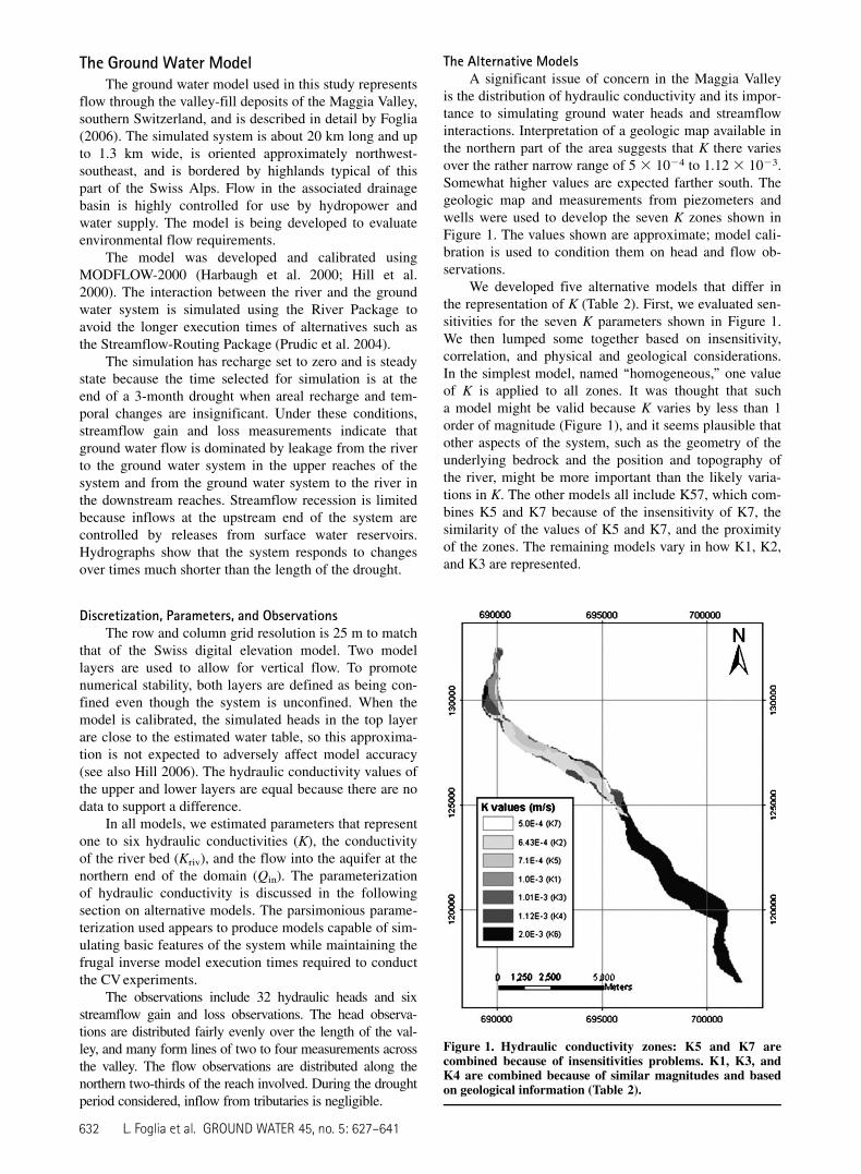
is the distribution of hydraulic conductivity and its impor-tance to simulating ground water heads and streamflowinteractions. Interpretation of a geologic map available inthe northern part of the area suggests that K there variesover the rather narrow range of 5 3 1024 to 1.12 3 1023.Somewhat higher values are expected farther south. Thegeologic map and measurements from piezometers andwells were used to develop the seven K zones shown inFigure 1. The values shown are approximate; model cali-bration is used to condition them on head and flow ob-servations.

We developed five alternative models that differ inthe representation of K (Table 2). First, we evaluated sen-sitivities for the seven K parameters shown in Figure 1.We then lumped some together based on insensitivity,correlation, and physical and geological considerations.In the simplest model, named ‘‘homogeneous,’’ one valueof K is applied to all zones. It was thought that sucha model might be valid because K varies by less than 1order of magnitude (Figure 1), and it seems plausible thatother aspects of the system, such as the geometry of theunderlying bedrock and the position and topography ofthe river, might be more important than the likely varia-tions in K. The other models all include K57, which com-bines K5 and K7 because of the insensitivity of K7, thesimilarity of the values of K5 and K7, and the proximityof the zones. The remaining models vary in how K1, K2,and K3 are represented.

Figure 1. Hydraulic conductivity zones: K5 and K7 arecombined because of insensitivities problems. K1, K3, andK4 are combined because of similar magnitudes and basedon geological information (Table 2).


ResultsWe present results obtained from the following steps:

1. Evaluate the five models using information criteria.

2. Identify 3HK (Table 2) as the best model.

3. Use the 3HK model to compare the linear statistics and

nonlinear CV statistics presented in the Methods. Con-

sider statistics that measure the importance of obser-

vations to parameter estimates and to simulated heads and

flows.

4. Apply CV for model selection and compare to the results

of step 1. Use models that are most complex (allK), sim-

plest (homogeneous), and best (3HK).

In steps 3 and 4, the CV experiments include (1)omitting individual observations and (2) omitting groupsof observations, where five groups are defined based ontheir location. Group 1 is close to the northern boundary;group 2 is within a wide, braided stream area locatedabout 7.5 km south of the northern end of the modeledarea; and groups 3, 4, and 5 form transects across the val-ley in its southern half (Figure 5-2 in Foglia 2006). Theleave-one-out CV method improves in accuracy if theprocedure is repeated for many observations or groups ofobservations (Chernick 1999, 105–106). We repeat theprocedure 43 times for all observations and groups of ob-servations (32 heads 1 6 flows 1 5 groups).

Model Selection Using AICc, BIC, and GCVTable 2 shows the AICc, BIC, and GCV information

criteria, and the model weight and the inverted evidenceratio. The values of the AICc, BIC, and GCV statisticssuggest that only the homogeneous model is clearly infe-rior, suggesting that variations in K are important. The3HK model is the ‘‘best’’ model in that it has the smallestvalues for AICc, BIC, and GCV. The inverted evidenceratio indicates that no other model is even half as proba-ble as the best 3HK model (all other inverted evidenceratios are less than 0.5).

Importance of Observations to Parameter Values

Nonlinear CV

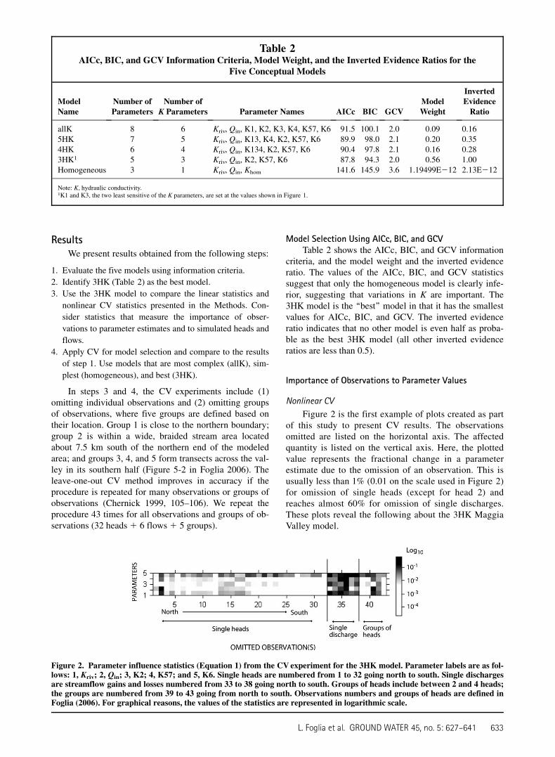
Figure 2 is the first example of plots created as partof this study to present CV results. The observationsomitted are listed on the horizontal axis. The affectedquantity is listed on the vertical axis. Here, the plottedvalue represents the fractional change in a parameterestimate due to the omission of an observation. This isusually less than 1% (0.01 on the scale used in Figure 2)for omission of single heads (except for head 2) andreaches almost 60% for omission of single discharges.These plots reveal the following about the 3HK MaggiaValley model.

Figure 2. Parameter influence statistics (Equation 1) from the CV experiment for the 3HK model. Parameter labels are as fol-lows: 1, Kriv; 2, Qin; 3, K2; 4, K57; and 5, K6. Single heads are numbered from 1 to 32 going north to south. Single dischargesare streamflow gains and losses numbered from 33 to 38 going north to south. Groups of heads include between 2 and 4 heads;the groups are numbered from 39 to 43 going from north to south. Observations numbers and groups of heads are defined inFoglia (2006). For graphical reasons, the values of the statistics are represented in logarithmic scale.

Table 2AICc, BIC, and GCV Information Criteria, Model Weight, and the Inverted Evidence Ratios for the

Five Conceptual Models

ModelName

Number ofParameters

Number ofK Parameters Parameter Names AICc BIC GCV

ModelWeight

InvertedEvidenceRatio

allK 8 6 Kriv, Qin, K1, K2, K3, K4, K57, K6 91.5 100.1 2.0 0.09 0.165HK 7 5 Kriv, Qin, K13, K4, K2, K57, K6 89.9 98.0 2.1 0.20 0.354HK 6 4 Kriv, Qin, K134, K2, K57, K6 90.4 97.8 2.1 0.16 0.283HK1 5 3 Kriv, Qin, K2, K57, K6 87.8 94.3 2.0 0.56 1.00Homogeneous 3 1 Kriv, Qin, Khom 141.6 145.9 3.6 1.19499E212 2.13E212

Note: K, hydraulic conductivity.1K1 and K3, the two least sensitive of the K parameters, are set at the values shown in Figure 1.


1. Unexpectedly, the observations tend to be most important to

hydraulic conductivity K6 (parameter 5 in Figure 2). We ex-

pected the observations to be most important to Kriv (param-

eter 1) because of the strong river-aquifer interactions in this

system. K6 is important because (1) K6 equals the hydraulic

conductivity of the entire downstream half of the domain

(downstream from head 18) and, therefore, controls flow

leaving the system through the river in the downstream half

of the system and (2) the last flow observation available (38

in Figure 2) is located at the upstream end of the zone char-

acterized by K6, so that the distribution of flow leaving the

system is poorly constrained. A test not presented here

shows that adding a new flow observation at the southern

end of the ground water domain makes head observations in

the south more important to Kriv.

2. The only head observation clearly important to most pa-

rameters is number 2. Head 2 is close to the northern flow

boundary condition and only a few meters from the river;

Figure 2 shows that it is important to parameters Kriv, Qin,

K57, and K6. In general, it exerts considerable control

over the water table in the north and the distribution of

flow into the system.

3. The discharge measurements are more important than

heads.

4. The most important groups of head observations omitted

are groups 3 and 4, which are located centrally within the

K6 zone.

The first three are used as comparison criteria for thelinear statistics. The fourth is not used because the linearstatistics are not used to test groups of observations.

Linear Statistics

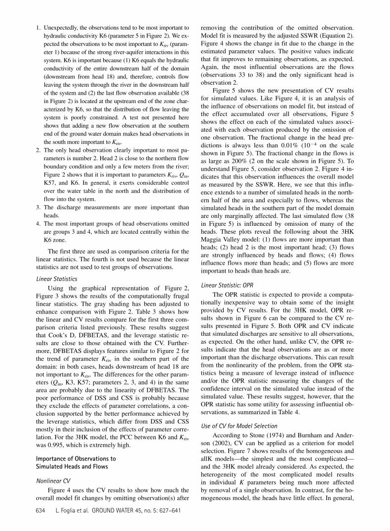
Using the graphical representation of Figure 2,Figure 3 shows the results of the computationally frugallinear statistics. The gray shading has been adjusted toenhance comparison with Figure 2. Table 3 shows howthe linear and CV results compare for the first three com-parison criteria listed previously. These results suggestthat Cook’s D, DFBETAS, and the leverage statistic re-sults are close to those obtained with the CV. Further-more, DFBETAS displays features similar to Figure 2 forthe trend of parameter Kriv in the southern part of thedomain: in both cases, heads downstream of head 18 arenot important to Kriv. The differences for the other param-eters (Qin, K3, K57; parameters 2, 3, and 4) in the samearea are probably due to the linearity of DFBETAS. Thepoor performance of DSS and CSS is probably becausethey exclude the effects of parameter correlations, a con-clusion supported by the better performance achieved bythe leverage statistics, which differ from DSS and CSSmostly in their inclusion of the effects of parameter corre-lation. For the 3HK model, the PCC between K6 and Kriv

was 0.995, which is extremely high.

Importance of Observations toSimulated Heads and Flows

Nonlinear CV

Figure 4 uses the CV results to show how much theoverall model fit changes by omitting observation(s) after

removing the contribution of the omitted observation.Model fit is measured by the adjusted SSWR (Equation 2).Figure 4 shows the change in fit due to the change in theestimated parameter values. The positive values indicatethat fit improves to remaining observations, as expected.Again, the most influential observations are the flows(observations 33 to 38) and the only significant head isobservation 2.

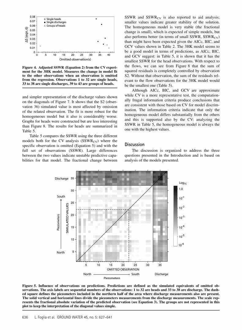
Figure 5 shows the new presentation of CV resultsfor simulated values. Like Figure 4, it is an analysis ofthe influence of observations on model fit, but instead ofthe effect accumulated over all observations, Figure 5shows the effect on each of the simulated values associ-ated with each observation produced by the omission ofone observation. The fractional change in the head pre-dictions is always less than 0.01% (1024 on the scaleshown in Figure 5). The fractional change in the flows isas large as 200% (2 on the scale shown in Figure 5). Tounderstand Figure 5, consider observation 2. Figure 4 in-dicates that this observation influences the overall modelas measured by the SSWR. Here, we see that this influ-ence extends to a number of simulated heads in the north-ern half of the area and especially to flows, whereas thesimulated heads in the southern part of the model domainare only marginally affected. The last simulated flow (38in Figure 5) is influenced by omission of many of theheads. These plots reveal the following about the 3HKMaggia Valley model: (1) flows are more important thanheads; (2) head 2 is the most important head; (3) flowsare strongly influenced by heads and flows; (4) flowsinfluence flows more than heads; and (5) flows are moreimportant to heads than heads are.

Linear Statistic: OPR

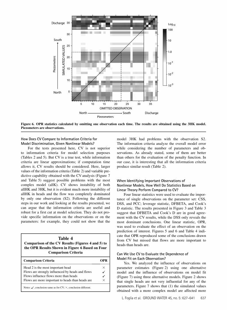
The OPR statistic is expected to provide a computa-tionally inexpensive way to obtain some of the insightprovided by CV results. For the 3HK model, OPR re-sults shown in Figure 6 can be compared to the CV re-sults presented in Figure 5. Both OPR and CV indicatethat simulated discharges are sensitive to all observations,as expected. On the other hand, unlike CV, the OPR re-sults indicate that the head observations are as or moreimportant than the discharge observations. This can resultfrom the nonlinearity of the problem, from the OPR sta-tistics being a measure of leverage instead of influenceand/or the OPR statistic measuring the changes of theconfidence interval on the simulated value instead of thesimulated value. These results suggest, however, that theOPR statistic has some utility for assessing influential ob-servations, as summarized in Table 4.

Use of CV for Model Selection

According to Stone (1974) and Burnham and Ander-son (2002), CV can be applied as a criterion for modelselection. Figure 7 shows results of the homogeneous andallK models—the simplest and the most complicated—and the 3HK model already considered. As expected, theheterogeneity of the most complicated model resultsin individual K parameters being much more affectedby removal of a single observation. In contrast, for the ho-mogeneous model, the heads have little effect. In general,


heads have less effect than flows, and this is consistent forthe three models and with what is shown in Figure 4. Thehead observations in the downstream part of the domain(observations 18 to 32) are not affected as much bychanging the hydraulic conductivity distribution because

in the 3HK and allK models the local hydraulic conduc-tivity, K6, is applied to the same extensive part of themodel.

Figure 8 shows the CV weighted residuals (Equation 4)for the streamflow observations. Figure 8 is a different

Figure 3. Linear statistics that measure the importance of observations to parameters. (a) DSS (Equation A5), (a1) CSS(Equation A6), (b) DFBETAS (Equation A8), (c) Cook’s D (Equation A7), and (d) leverage statistics (Equation A9). Parameterlabels are as follows: 1, Kriv; 2, Qin; 3, K2; 4, K57; and 5, K6. Omitted observations are numbered as for Figure 2.

Table 3Comparison of the CV Results (Figure 2) to the Linear Statistic Results (Figure 3) Based on

Three Comparison Criteria

Linear Statistics

Comparison Criteria DSS DFBETAS Cook’s D Leverage CSS

Observations most important to K6 3 — — 3

Head 2 most important head 3 —Flows more important than heads —

Notes: conclusion same as for CV; 3 conclusion different; — not applicable.


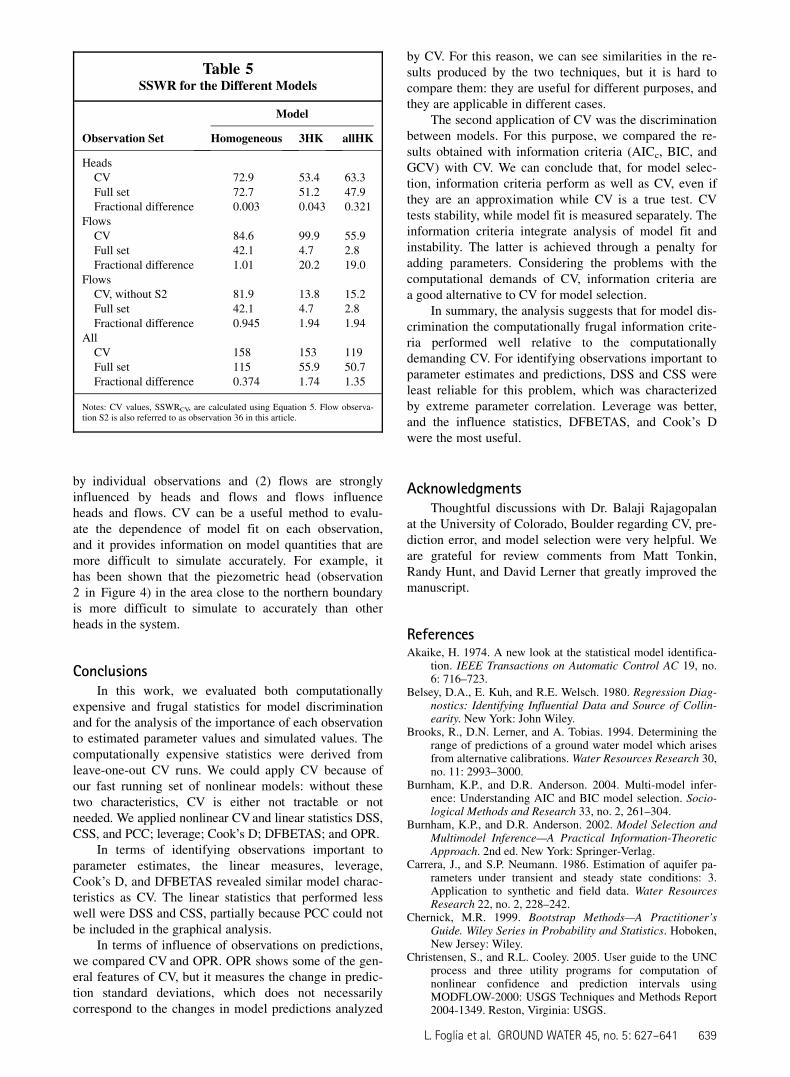
and simpler representation of the discharge values shownon the diagonals of Figure 7. It shows that the S2 (obser-vation 36) simulated value is most affected by omissionof the related observation. The fit is more robust for thehomogeneous model but it also is considerably worse.Graphs for heads were constructed but are less interestingthan Figure 8. The results for heads are summarized inTable 5.

Table 5 compares the SSWR using the three differentmodels both for the CV analysis (SSWRCV) where thespecific observation is omitted (Equation 5) and with thefull set of observations (SSWR). Large differencesbetween the two values indicate unstable predictive capa-bilities for that model. The fractional change between

SSWR and SSWRCV is also reported to aid analysis;smaller values indicate greater stability of the solution.The homogeneous model is very stable (the fractionalchange is small), which is expected of simple models, butalso performs better (in terms of small SSWR, SSWRCV)than might have been expected given the AICc, BIC, andGCV values shown in Table 2. The 3HK model seems tobe a good model in terms of predictions, as AICc, BIC,and GCV suggest: in Table 5, it is shown that it has thesmallest SSWR for the head observations. With respect tothe flows, we can see from Figure 8 that the sum ofsquared residuals is completely controlled by observationS2. Without that observation, the sum of the residuals rel-evant to the flow observations for the 3HK model wouldbe the smallest one (Table 5).

Although AICc, BIC, and GCV are approximatewhile CV is a more representative test, the computation-ally frugal information criteria produce conclusions thatare consistent with those based on CV for model discrim-ination. The information criteria indicate that only thehomogeneous model differs substantially from the othersand this is supported also by the CV: analyzing theSSWR in Table 5, the homogeneous model is always theone with the highest values.

DiscussionThe discussion is organized to address the three

questions presented in the Introduction and is based onanalysis of the models presented.

Figure 5. Influence of observations on predictions. Predictions are defined as the simulated equivalents of omitted ob-servations. The axis labels are sequential numbers of the observations: 1 to 32 are heads and 33 to 38 are discharge. The dash-ed square defines the piezometers included in the northern half of the area where discharge measurements also are present.The solid vertical and horizontal lines divide the piezometers measurements from the discharge measurements. The scale rep-resents the fractional absolute variation of the predicted observation (see Equation 3). The groups are not represented in thisplot to keep the interpretation of the diagonal values simple.

Figure 4. Adjusted SSWR (Equation 2) from the CV experi-ment for the 3HK model. Measures the change in model fitto the other observations when an observation is omittedfrom the regression. Observations 1 to 32 are single heads,33 to 38 are single discharges, 39 to 43 are groups of heads.


How Does CV Compare to Information Criteria forModel Discrimination, Given Nonlinear Models?

For the tests presented here, CV is not superiorto information criteria for model selection purposes(Tables 2 and 5). But CV is a true test, while informationcriteria are linear approximations; if computation timeallows it, CV results should be considered. Here, largervalues of the information criteria (Table 2) and variable pre-dictive capability obtained with the CV analysis (Figure 7and Table 5) suggest possible problems with the mostcomplex model (allK). CV shows instability of bothallHK and 3HK, but it is evident much more instability ofallHK in heads and the flow was completely dominatedby only one observation (S2). Following the differentsteps in our work and looking at the results presented, wecan argue that the information criteria are useful androbust for a first cut at model selection. They do not pro-vide specific information on the observations or on theparameters: for example, they could not show that the

model 3HK had problems with the observation S2.The information criteria analyze the overall model errorwhile considering the number of parameters and ob-servations. As already stated, some of them are betterthan others for the evaluation of the penalty function. Inour case, it is interesting that all the information criteriaproduce similar result (Table 2).

When Identifying Important Observations ofNonlinear Models, How Well Do Statistics Based onLinear Theory Perform Compared to CV?

Four linear statistics were used to evaluate the impor-tance of single observations on the parameter set: CSS,DSS, and PCC; leverage statistic, DFBETA, and Cook’sD statistic. The results presented in Figure 3 and Table 3suggest that DFBETA and Cook’s D are in good agree-ment with the CV results, while the DSS only reveals themost dominant conclusions. One linear statistic, OPR,was used to evaluate the effect of an observation on theprediction of interest. Figures 5 and 6 and Table 4 indi-cate that OPR reproduced some of the conclusions drawnfrom CV but missed that flows are more important toheads than heads are.

Can We Use CV to Evaluate the Dependence ofModel Fit on Each Observation?

Yes. We analyzed the influence of observations onparameter estimates (Figure 2) using one alternativemodel and the influence of observations on model fit(Figure 7) using three alternative models. Figure 2 showsthat single heads are not very influential for any of theparameters. Figure 7 shows that (1) the simulated valuesobtained with a more complex model are affected more

Figure 6. OPR statistics calculated by omitting one observation each time. The results are obtained using the 3HK model.Piezometers are observations.

Table 4Comparison of the CV Results (Figures 4 and 5) tothe OPR Results Shown in Figure 6 Based on Four

Comparison Criteria

Comparison Criteria OPR

Head 2 is the most important head 3

Flows are strongly influenced by heads and flowsFlows influence flows more than headsFlows are more important to heads than heads are 3

Notes: , conclusion same as for CV;3, conclusion different.


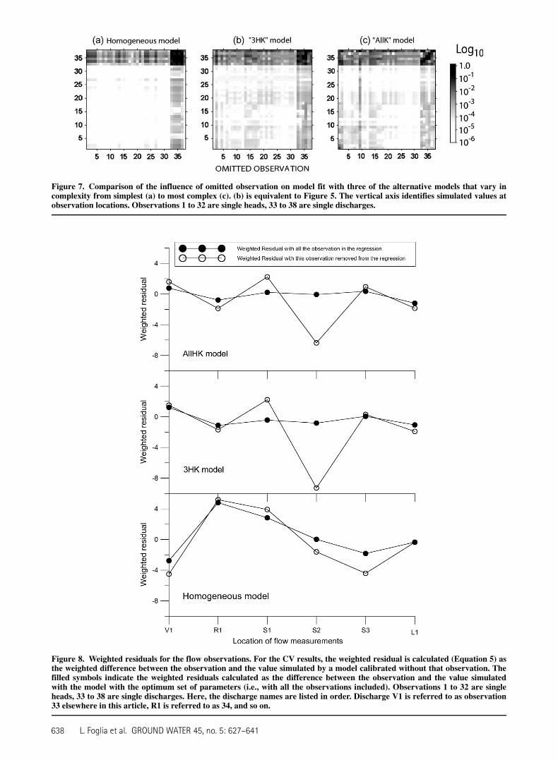
Figure 7. Comparison of the influence of omitted observation on model fit with three of the alternative models that vary incomplexity from simplest (a) to most complex (c). (b) is equivalent to Figure 5. The vertical axis identifies simulated values atobservation locations. Observations 1 to 32 are single heads, 33 to 38 are single discharges.

Figure 8. Weighted residuals for the flow observations. For the CV results, the weighted residual is calculated (Equation 5) asthe weighted difference between the observation and the value simulated by a model calibrated without that observation. Thefilled symbols indicate the weighted residuals calculated as the difference between the observation and the value simulatedwith the model with the optimum set of parameters (i.e., with all the observations included). Observations 1 to 32 are singleheads, 33 to 38 are single discharges. Here, the discharge names are listed in order. Discharge V1 is referred to as observation33 elsewhere in this article, R1 is referred to as 34, and so on.


by individual observations and (2) flows are stronglyinfluenced by heads and flows and flows influenceheads and flows. CV can be a useful method to evalu-ate the dependence of model fit on each observation,and it provides information on model quantities that aremore difficult to simulate accurately. For example, ithas been shown that the piezometric head (observation2 in Figure 4) in the area close to the northern boundaryis more difficult to simulate to accurately than otherheads in the system.

ConclusionsIn this work, we evaluated both computationally

expensive and frugal statistics for model discriminationand for the analysis of the importance of each observationto estimated parameter values and simulated values. Thecomputationally expensive statistics were derived fromleave-one-out CV runs. We could apply CV because ofour fast running set of nonlinear models: without thesetwo characteristics, CV is either not tractable or notneeded. We applied nonlinear CVand linear statistics DSS,CSS, and PCC; leverage; Cook’s D; DFBETAS; and OPR.

In terms of identifying observations important toparameter estimates, the linear measures, leverage,Cook’s D, and DFBETAS revealed similar model charac-teristics as CV. The linear statistics that performed lesswell were DSS and CSS, partially because PCC could notbe included in the graphical analysis.

In terms of influence of observations on predictions,we compared CV and OPR. OPR shows some of the gen-eral features of CV, but it measures the change in predic-tion standard deviations, which does not necessarilycorrespond to the changes in model predictions analyzed

by CV. For this reason, we can see similarities in the re-sults produced by the two techniques, but it is hard tocompare them: they are useful for different purposes, andthey are applicable in different cases.

The second application of CV was the discriminationbetween models. For this purpose, we compared the re-sults obtained with information criteria (AICc, BIC, andGCV) with CV. We can conclude that, for model selec-tion, information criteria perform as well as CV, even ifthey are an approximation while CV is a true test. CVtests stability, while model fit is measured separately. Theinformation criteria integrate analysis of model fit andinstability. The latter is achieved through a penalty foradding parameters. Considering the problems with thecomputational demands of CV, information criteria area good alternative to CV for model selection.

In summary, the analysis suggests that for model dis-crimination the computationally frugal information crite-ria performed well relative to the computationallydemanding CV. For identifying observations important toparameter estimates and predictions, DSS and CSS wereleast reliable for this problem, which was characterizedby extreme parameter correlation. Leverage was better,and the influence statistics, DFBETAS, and Cook’s Dwere the most useful.

AcknowledgmentsThoughtful discussions with Dr. Balaji Rajagopalan

at the University of Colorado, Boulder regarding CV, pre-diction error, and model selection were very helpful. Weare grateful for review comments from Matt Tonkin,Randy Hunt, and David Lerner that greatly improved themanuscript.

ReferencesAkaike, H. 1974. A new look at the statistical model identifica-

tion. IEEE Transactions on Automatic Control AC 19, no.6: 716–723.

Belsey, D.A., E. Kuh, and R.E. Welsch. 1980. Regression Diag-nostics: Identifying Influential Data and Source of Collin-earity. New York: John Wiley.

Brooks, R., D.N. Lerner, and A. Tobias. 1994. Determining therange of predictions of a ground water model which arisesfrom alternative calibrations. Water Resources Research 30,no. 11: 2993–3000.

Burnham, K.P., and D.R. Anderson. 2004. Multi-model infer-ence: Understanding AIC and BIC model selection. Socio-logical Methods and Research 33, no. 2, 261–304.

Burnham, K.P., and D.R. Anderson. 2002. Model Selection andMultimodel Inference—A Practical Information-TheoreticApproach. 2nd ed. New York: Springer-Verlag.

Carrera, J., and S.P. Neumann. 1986. Estimation of aquifer pa-rameters under transient and steady state conditions: 3.Application to synthetic and field data. Water ResourcesResearch 22, no. 2, 228–242.

Chernick, M.R. 1999. Bootstrap Methods—A Practitioner’sGuide. Wiley Series in Probability and Statistics. Hoboken,New Jersey: Wiley.

Christensen, S., and R.L. Cooley. 2005. User guide to the UNCprocess and three utility programs for computation ofnonlinear confidence and prediction intervals usingMODFLOW-2000: USGS Techniques and Methods Report2004-1349. Reston, Virginia: USGS.

Table 5SSWR for the Different Models

Model

Observation Set Homogeneous 3HK allHK

HeadsCV 72.9 53.4 63.3Full set 72.7 51.2 47.9Fractional difference 0.003 0.043 0.321

FlowsCV 84.6 99.9 55.9Full set 42.1 4.7 2.8Fractional difference 1.01 20.2 19.0

FlowsCV, without S2 81.9 13.8 15.2Full set 42.1 4.7 2.8Fractional difference 0.945 1.94 1.94

AllCV 158 153 119Full set 115 55.9 50.7Fractional difference 0.374 1.74 1.35

Notes: CV values, SSWRCV, are calculated using Equation 5. Flow observa-tion S2 is also referred to as observation 36 in this article.


Christensen, S., and R.L. Cooley. 1999. Evaluation of predictionintervals for expressing uncertainties in ground water flowmodel predictions. Water Resources Research 35, no. 9:2627–2639.

Cook, R.D., and S. Weisberg. 1982. Residuals and influence inregression. Monogr. Stat. Appl. Probability 18. New York:Chapman and Hall.

Cooley, R.L. 2004. A theory for modeling ground-water flow inheterogeneous media. USGS Professional Paper 1679.Reston, Virginia: USGS.

Cooley, R.L., and R.L. Naff. 1990. Regression modelingof ground-water flow. USGS Techniques in Water-Resources Investigations, book 3, chap. B4. Reston,Virginia: USGS.

Craven, P., and G. Whaba. 1979. Smoothing noisy data withspline functions: Estimating the correct degree of smooth-ing by the method of generalized cross-validation. Numeri-sche Mathematik 31, 377–403.

Draper, N.R., and H. Smith. 1998. Applied Regression Analysis,3rd ed. New York: John Wiley and Sons.

Efron, B. 1982. The Jackknife, the Bootstrap, and other resam-pling plans. Monograph No. 38. Philadelphia, Pennsyl-vania: SIAM NSF-CBMS.

Foglia, L. 2006. Alternative groundwater models to investigateriver-aquifer interactions in an environmentally activealpine floodplain. PhD dissertation. Institute for Environ-mental Engineering, ETH Zurich, Switzerland.

Good, P.I. 2001. Resampling Methods—A Practical Guide toData Analysis. Boston, Massachusetts: Birkhauser.

Harbaugh, A.W., E.R. Banta, M.C. Hill, and M.G. McDonald.2000. MODFLOW-2000, The U.S. Geological Surveymodular ground-water model—Users guide to modulariza-tion concepts and the ground-water flow process. USGSOpen-File Report 00-92. Reston, Virginia: USGS.

Helsel, D.R., and R.M. Hirsh. 2002. Statistical methods in waterresources. U.S. Geological Survey Techniques in Water Re-sources, Book 4, Chapter A3. Available at: http://pubs.water.usgs.gov/twri4a3.

Hill, M.C. 2006. The practical use of simplicity in de-veloping ground water models. Ground Water 44, no. 6:775–781.

Hill, M.C. 1998. Methods and guidelines for groundwater modelcalibration. USGS Water-Resources Investigations Report98-4005. Reston, Virginia: USGS.

Hill, M.C., and C.R. Tiedeman. 2007. Effective Calibration ofGroundwater Models, with Analysis of Data, Sensitivities, Pre-dictions, and Uncertainty. New York: John Wiley and Sons.

Hill, M.C., E.R. Banta, A.W. Harbaugh, and E.R. Anderman.2000. MODFLOW-2000, The U.S. Geological Surveymodular ground-water model, User’s guide to the observa-tion, sensitivity, and parameter-estimation processes. USGSOpen-File Report 00-184. Reston, Virginia: USGS.

Hunt, R.J., D.T. Feinstein, C.D. Pint, and M.P. Anderson, 2006.The importance of diverse data types to calibrate a water-shed model of the Trout Lake Basin, Northern Wisconsin,USA. Journal of Hydrology 321, no. 1–4: 286–296.

Isaaks, E., and R. Srivastava. 1989. An Introduction to AppliedGeostatistics. New York: Oxford University Press.

Moore, C., and J. Doherty. 2005. Role of the calibration processin reducing model predictive error. Water ResourcesResearch 41, W05020, doi: 10.1029/2004WR003501.

Perona, P., A. Porporato, and L. Ridolfi. 2000. On the trajectorymethod for the reconstruction of differential equations fromtime series. Nonlinear Dynamics 23, no. 1: 13–33.

Poeter, E.P., and D.R. Anderson. 2005. Multi-model ranking andinference in ground water modeling. Ground Water 43, no.4: 597–605.

Poeter, E.P., and M.C. Hill. 2007. MMA-computer code for multi-model analysis. USGS Techniques and Methods TM6E-3.Reston, Virginia: USGS.

Prudic, D.E., L.F. Konikow, and E.R. Banta, 2004. A newstreamflow-routing (SFR1) package to simulate stream-

aquifer interaction with MODFLOW-2000. USGS Open-File Report 2004-1042. Reston, Virginia: USGS.

Regonda, S.K., B. Rajagopalan, U. Lall, M. Clark, and Y.I.Moon. 2005. Local polynomial method for ensemble fore-cast of time series. Nonlinear Processes in Geophysics 12,no. 3: 397–406.

Saltelli, A., S.K.P.-S. Chan, and E.M. Scott. 2000. SensitivityAnalysis. Hoboken, New Jersey: John Wiley and Sons.

Schwarz, G. 1978. Estimating the dimension of a model. Annalsof Statistics 6, 461–464.

Shao, J. 1993. Linear model selection by cross-validation.Journal of the American Statistical Association 88, no. 422:486–494.

Stone, M. 1974. Cross-validatory choice and assessment of sta-tistical predictions. Journal of the Royal Statistical Society,Series B (Methodological) 36, no. 2: 111–147.

Tiedeman, C.R., D.M. Ely, M.C. Hill, and G.M. O’Brien. 2004.A method for evaluating the importance of system stateobservations to model predictions, with application to theDeath Valley regional groundwater flow system. WaterResources Research, no. 40, 1–17.

Tonkin, M.J., and S.P. Larson. 2002. Kriging water levels witha regional-linear and point-logarithmic drift. Ground Water40, no. 2: 185–193.

Tonkin, M.J., C.R. Tiedeman, D.M. Ely, and M.C. Hill. 2007.Documentation of OPR-PPR, a computer program for as-sessing data importance to model predictions using linearstatistics. USGS Techniques and Methods TM6-E2. Reston,Virginia: USGS.

Wu, C.F.J. 1986. Jackknife, Bootstrap and other resamplingmethods in regression analysis. The Annals of Statistics 14,no. 4: 1261–1295.

Yager, R.M. 2004. Effects of model sensitivity and nonlinearityon nonlinear regression of ground water flow. GroundWater 42, no. 3: 390–400.

Yager, R.M. 1998. Detecting influential observations in non-linear regression modeling of ground water flow. WaterResources Research 34, no. 7: 1623–1633.

Appendix 1

Information CriteriaAIC and AICc are defined as:

AIC ¼ nlogðr2Þ 1 2k k ffi n ðA1Þ

AICc ¼ nlogðr2Þ 1 2k 1

�2kðk 1 1Þn 2 k 2 1

�n

k,40 ðA2Þ

where r2 is the maximum likelihood estimate of theresidual variance, calculated as SSWR/n; SSWR is theweighted residual sum of squares (Poeter and Anderson2005; Burnham and Anderson 2002, 12); n is the numberof observations; k is the number of estimated parametersfor the model; if for any model n/k < 40, Burnham andAnderson (2002) suggest AICc be used.

BIC was derived by Schwarz (1978), as follows:

BIC ¼ nlogðr2Þ 1 klogðnÞ ðA3Þ

where the symbols are defined as for Equation 6. UnlikeBIC, AIC and AICc are not aimed at finding the ‘‘true’’model and provide a greater penalty as parameters areadded.

GCV is defined as follows:


GCV ¼Pni¼1

e2in =�1 2 k

n

�2nlogðGCVÞ ¼ nlogðr2Þ 2 2n½logðn 2 kÞ 2 logðnÞ�

ðA4Þ

where ei is the residual for the observation i (here, theweighted residual). This measure is widely used forensemble forecast of time series (Regonda et al. 2005).

Linear Statistics

DSS, CSS, and PCCAssuming a diagonal weight matrix, DSS is calcu-

lated as follows:

dssij ¼ ð@y9i=@bjÞjbbjx1=2ii ðA5Þ

where y9 is a simulated value; bj is the jth estimatedparameter; (@y9i/@bj) is the derivative, or sensitivity, of thesimulated value associated with the ith observation withrespect to the jth parameter, and is evaluated at the set ofparameter values in b; b is a vector of the parameter val-ues; xii is the weight for the ith observation, assuminga diagonal weight matrix as in the previous equations(Hill and Tiedeman 2007).

The CSS for each parameter is calculated as follows:

cssj ¼Xni¼1

h�dssij

�2jb=ni1=2

ðA6Þ

where n is the number of observations.

Cook’s D and DFBETASCook’s D is calculated as (Cook and Weisberg 1982;

Yager 1998) follows:

Di ¼ðbðiÞ2b9ÞT

hr2ðXTxXÞ21

i21

ðbðiÞ 2 b9Þp

¼ 1

pr2i

hii1 2 hii ðA7Þ

where p is the actual number of parameters, b(i) is the setof parameter values optimized with the observation iomitted, b9 is the set of parameter values optimized usingall observations, r2 is the variance of the regression, X isthe sensitivity matrix, (XTxX)21 is the square symmetricparameter variance-covariance matrix, x is the matrix ofweights on observations used in the calibration, ri is theweighted standardized residual corresponding to observa-tion i, hii is a diagonal element of the hat matrix (Hill andTiedeman 2007).

Belsey et al. (1980) define DFBETAS as follows:

DFBETASij ¼ðb9i 2 b9jðiÞÞ

sðiÞffiffiffiffiffiffiffiffiffiffiffiffiffiffiffiffiffiffiffiffiffi½XTxX�21

jj

q¼ cji�PND

k¼1

c2jk

�1=2

fisðiÞð1 2 hiiÞ

ðA8Þ

where b9j is the optimized value of the jth estimatedparameter using all observations, b9j(i) is the optimizedvalue of the jth estimated parameter when observation i isremoved, s(i) is the estimate of r chosen to make thedenominator statistically independent of the numeratorunder normal theory, cji is an entry of the matrix productC ¼ (XTxX)21x1/2XT (Helsel and Hirsch 2002; Hill andTiedeman 2007), and fi is the ith weighted residual of theregression with all observations.

All the other symbols were already defined afterEquation 12.

Leverage StatisticsIt is measured using the following equation (Hill and

Tiedeman 2007):

hii ¼ xTi ðXTxXÞ21xi ðA9Þ

where hii is the leverage for observation i and xTi is the ithrow of the X matrix

OPRThe OPR statistic is based on the equation for linear

statistical inference for calculating standard deviations onpredictions (Draper and Smith 1998; Hill and Tiedeman2007):

sz9‘ ¼hs2�ZðXTxXÞ21

ZT�‘‘

i1=2ðA10Þ

where sz9‘ is the standard deviation of the ‘th prediction,z9‘; s2 is the calculated error variance; and Z is the matrixof sensitivities of the predictions with respect to themodel parameters, with elements equal to @z9‘=@bj.

OPR measures the effect of an observation on thestandard deviation of a prediction. Like DFBETAS, thisis done by deleting a row of the X matrix correspondingto a particular observation and calculating the resultingchange in the prediction interval. To produce a convenientmeasure of relative observation importance that can beeasily evaluated and mapped or plotted, the percentchange in prediction uncertainty is calculated as follows:

ðsz9‘ðiÞ=sz9‘Þ 2 1:03 100 ðA11Þ

where sz9‘ðiÞis the standard deviation of the ‘th simulatedvalue, z9‘, with the ith observation removed.


Documents

Testing Alternative Ground Water Models Using Cross-Validation and Other Methods