Texas AgriLife Research golden-cheeked warbler surveys

979.845-1851 irnr@tamu.edu

irnr.tamu.edu

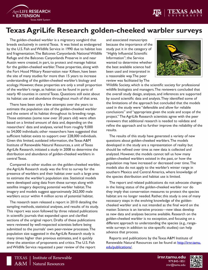
The golden-cheeked warbler is a migratory songbird that breeds exclusively in central Texas. It was listed as endangered by the U.S. Fish and Wildlife Service in 1990 due to habitat loss and fragmentation. The Balcones Canyonlands National Wildlife Refuge and the Balcones Canyonlands Preserve in and near Austin were created, in part, to protect and manage habitat for the golden-cheeked warbler. These properties, along with the Fort Hood Military Reservation near Killeen, have been the site of many studies for more than 15 years to increase understanding of the golden-cheeked warbler’s biology and ecology. However, these properties are only a small proportion of the warbler’s range, as habitat can be found in parts of nearly 40 counties in central Texas. Questions still exist about its habitat use and abundance throughout much of that area.

There have been only a few attempts over the years to estimate the population size of the golden-cheeked warbler and the extent of its habitat throughout its breeding range. Those estimates (some now over 20 years old) were often based on a limited amount of data and, depending on the researchers’ data and analyses, varied from roughly 9,000 to 54,000 individuals; other researchers have suggested that sufficient habitat exists to support over 228,000 individuals. Given this limited, outdated information, the Texas A&M Institute of Renewable Natural Resources, a unit of Texas AgriLife Research, initiated a study in 2008 to determine the distribution and abundance of golden-cheeked warblers in central Texas.

Compared to other studies on the golden-cheeked warbler, the AgriLife Research study was the first to survey for the presence of warblers and their habitat over such a large area to estimate the warbler’s population size. Statistical models were developed using data from these surveys along with satellite imagery depicting potential warbler habitat. The imagery and models suggest approximately 262,000 male warblers occur within 4 million acres of potential habitat.

The research team released a report in 2010 detailing the sampling methods, statistical analyses, and results of its study. This report was soon followed by three related publications in scientific journals that expanded upon and clarified sections of the original report. Drafts of these publications were reviewed by well-respected scientists before being submitted to the journals’ own peer-review processes. The population size suggested in the AgriLife Research study is many times higher than previous estimates, and it quickly drew the attention of proponents and critics. The U.S. Fish and Wildlife Service requested a peer review of the report

and associated manuscripts because the importance of the study put it in the category of “Highly Influential Scientific Information”; the Service wanted to determine whether the best available science had been used and interpreted in a reasonable way. The peer review was facilitated by The Wildlife Society, which is the scientific society for professional wildlife biologists and managers. The reviewers concluded that the overall study design, analyses, and inferences are supported by sound scientific data and analysis. They identified some of the limitations of the approach but concluded that the models used in the study were “defensible and allow for reliable conclusions” and “appropriate given the scale and scope of the project.” The AgriLife Research scientists agree with the peer reviewers that additional research is needed to validate and refine the approach and to further improve the reliability of the results.

The results of this study have generated a variety of new questions about golden-cheeked warblers. The models developed in the study are a representation of reality but should be refined over time as new data is collected and analyzed. However, the models cannot tell us how many golden-cheeked warblers existed in the past, or how the population may have increased or decreased over time. The models also do not apply to the warbler’s winter range in southern Mexico and Central America, where knowledge of the species distribution and habitat use is limited.

The report and related publications do not advocate changes in the listing status of the golden-cheeked warbler nor do they imply that conservation measures to protect the species habitat are no longer needed. Rather, this study is one of many necessary steps in the evolving knowledge of the golden-cheeked warbler and is not intended as the final word on the matter. Science is an iterative process—new ideas develop as new data and analyses become available. Research on the golden-cheeked warbler is no exception, and focusing on a different approach to understanding the species (e.g., range-wide surveys in addition to site-specific studies) can help advance that process.

Reports and publications by the Texas A&M Institute of Renewable Natural Resources can be found at http://irnr.tamu.edu/publications/.

Research Article

Estimating Breeding Season Abundance ofGolden-Cheeked Warblers in Texas, USA

HEATHER A. MATHEWSON,1 Texas A&M Institute of Renewable Natural Resources, 1500 Research Parkway, Suite 110, Texas A&MUniversity, College Station, TX 77843, USA

JULIE E. GROCE, Texas A&M Institute of Renewable Natural Resources, 2632 Broadway, Suite 301 S., Texas A&M University, San Antonio,TX 78215, USA

TIFFANY M. MCFARLAND, Texas A&M Institute of Renewable Natural Resources, 1500 Research Parkway, Suite 110, Texas A&M University,College Station, TX 77843, USA

MICHAEL L. MORRISON, Department of Wildlife and Fisheries Sciences, 210 Nagle Hall, Texas A&M University, CollegeStation, TX 77843, USA

J. CAL NEWNAM, Texas Department of Transportation, P.O. Box 15426, Austin, TX 78761, USA

R. TODD SNELGROVE, Texas A&M Institute of Renewable Natural Resources, 1500 Research Parkway, Suite 110, Texas A&M University,College Station, TX 77843, USA

BRET A. COLLIER, Texas A&M Institute of Renewable Natural Resources, 1500 Research Parkway, Suite 110, Texas A&M University, CollegeStation, TX 77843, USA

R. NEAL WILKINS, Texas A&M Institute of Renewable Natural Resources, 1500 Research Parkway, Suite 110, Texas A&M University, CollegeStation, TX 77843, USA

ABSTRACT Population abundance estimates using predictive models are important for describing habitatuse and responses to population-level impacts, evaluating conservation status of a species, and for establishingmonitoring programs. The golden-cheeked warbler (Setophaga chrysoparia) is a neotropical migratory birdthat was listed as federally endangered in 1990 because of threats related to loss and fragmentation of itswoodland habitat. Since listing, abundance estimates for the species have mainly relied on localizedpopulation studies on public lands and qualitative-based methods. Our goal was to estimate breedingpopulation size of male warblers using a predictive model based on metrics for patches of woodland habitatthroughout the species’ breeding range. We first conducted occupancy surveys to determine range-widedistribution.We then conducted standard point-count surveys on a subset of the initial sampling locations toestimate density of males. Mean observed patch-specific density was 0.23 males/ha (95% CI ¼ 0.197–0.252,n ¼ 301). We modeled the relationship between patch-specific density of males and woodland patchcharacteristics (size and landscape composition) and predicted patch occupancy. The probability of patchoccupancy, derived from a model that used patch size and landscape composition as predictor variables whileaddressing effects of spatial relatedness, best predicted patch-specific density. We predicted patch-specificdensities as a function of occupancy probability and estimated abundance of male warblers across 63,616woodland patches accounting for 1.678 million ha of potential warbler habitat. Using a Monte Carlosimulation, our approach yielded a range-wide male warbler population estimate of 263,339 (95% CI:223,927–302,620). Our results provide the first abundance estimate using habitat and count data from asampling design focused on range-wide inference. Managers can use the resulting model as a tool to supportconservation planning and guide recovery efforts. � 2012 The Wildlife Society.

KEY WORDS abundance, density, endangered species, golden-cheeked warbler, point count, population estimate,Setophaga chrysoparia, Texas.

Abundance estimates are of particular importance for evalu-ating conservation status and determining recovery goals,establishing monitoring programs, describing habitat usepatterns, and assessing population-level impacts driven byanthropogenic and natural factors (Campbell et al. 2002,Scott et al. 2005, Fitzgerald et al. 2009, Sirami et al. 2010).Population size estimation is a challenge for most species, butapproaches integrating remotely sensed data with predictive

models can assist in predicting abundance at large spatialscales (Thompson 2002a, Fitzgerald et al. 2009). The gold-en-cheeked warbler (Setophaga chrysoparia) is a neotropicalmigratory songbird that breeds only in central Texas andwinters in the highlands of southern Mexico and CentralAmerica (Pulich 1976, Groce et al. 2010). In 1990, theUnited States Fish and Wildlife Service (USFWS) listedthe golden-cheeked warbler (hereafter warbler) as endan-gered and cited habitat loss and fragmentation as primarythreats (USFWS 1990, 1992). Warbler occurrence, density,and recruitment rates appear to decrease as the size ofhabitat patches and the amount of habitat in the surrounding

Received: 25 March 2011; Accepted: 28 November 2011

1E-mail: hamathewson@tamu.edu

The Journal of Wildlife Management; DOI: 10.1002/jwmg.352

Mathewson et al. �Warbler Population Abundance 1

landscape decline (DeBoer and Diamond 2006, Magnesset al. 2006, Peak 2007, Butcher et al. 2010, Collier et al.2010).Previously, approximations of golden-cheeked warbler

abundance within the breeding range were based on esti-mates of warbler density collected at a few (<20) study sitesand extrapolated based on projected extents of breedinghabitat (Pulich 1976, Wahl et al. 1990, Rowell et al.1995, Rappole et al. 2003; Table 1). Population estimateshave ranged between 9,644 and 32,032 individuals (Pulich1976, Wahl et al. 1990), whereas estimates of carryingcapacity have ranged from 64,520 to 228,426 individuals(Rowell et al. 1995, Rappole et al. 2003). Variation inpopulation estimates results from the methods used to esti-mate the extent of habitat, and assumptions regarding whatcharacteristics are representative of warbler habitat (Table 1).Our objective was to develop a range-wide estimate of

abundance for male warblers. We relied on a range-widemodel predicting patch level occupancy (Collier et al. 2012)to serve as our sampling frame. We then used point countsurveys to estimate patch-specific density of male warblers.We evaluated predictive relationships between patch-specificdensity and remotely sensedmetrics of habitat patches. Usingthese relationships, we combined our density estimates withthe range-wide occupancy model to yield estimates of malewarbler abundance across the species’ breeding range.

STUDY AREA

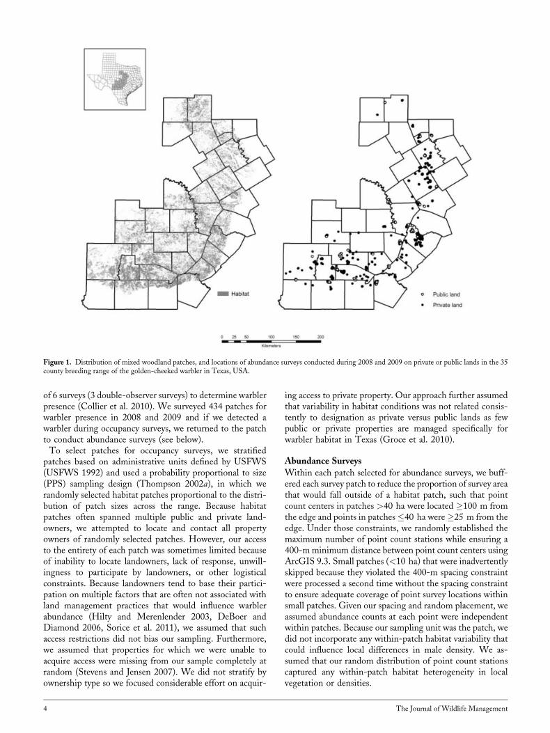
The golden-cheeked warbler breeding range is confined tocentral Texas, USA, on the eastern half of the EdwardsPlateau and the southern half of the Cross Timbers ecor-egions (Hatch et al. 1990).We conducted our research acrossthe breeding range on public and private properties in 35counties (USFWS 1992; Fig. 1). Our sampling units werepatches of potential warbler habitat, characterized as oak-juniper woodlands (Collier et al. 2010, 2012), and we defineda patch as a relatively homogenous unit of vegetation distinctfrom its surroundings (Kotliar and Wiens 1990). To guideus in determining survey locations in 2008, we used ahabitat classification developed by SWCA EnvironmentalConsultants (SWCA 2007) that delineated potential warblerhabitat as those patches having >50% canopy closure by amixture of mature or second-growth Ashe juniper (Juniperusashei) and deciduous hardwood trees based on 2004 NationalAgricultural Imagery Program color infrared digital imagery(1-m resolution). SWCA (2007) excluded patches <4 haunless immediately adjacent (unspecified distance) to otherpatches of potential habitat. SWCA’s restricted definition ofhabitat yielded 7,865 patches (approx. 552,000 ha) of po-tential habitat across the breeding range. Based on our fieldsurveys during 2008, as well as previous work within thissystem (Butcher et al. 2010, Collier et al. 2010), we found theSWCA (2007) classification narrowly defined warbler habi-tat; thus, we developed a broader classification of warblerhabitat patches for selecting survey sites in 2009 and forevaluating relationships between patch-specific densities andpatch metrics.

We delineated potential habitat using an unsupervisedclassification of woodlands from 2007 and 2008 cloud-freeLandsat 5 imagery collected during late spring (Morrisonet al. 2010). Using the ISODATA clustering algorithm inLeica ERDAS Imagine 9.3 (Intergraph Corporation,Norcross, GA), we grouped imagery spectral response pat-terns into 20 statistically different clusters. Using high reso-lution aerial photography from the National AgricultureImagery Program (NAIP; 2004 and 2006) and data collectedin the field, we identified those clusters that corresponded towoodland land cover, grouping all other land cover types asnon-habitat (e.g., wetlands, cropland, urban areas, water,barren, impervious surfaces, grassland). Several woodlandclusters were based on characteristics such as slope, aspect,shadows, and composition (e.g., evergreen or deciduous);however, because classification accuracy of these woodlandswas low and our intent was to sample woodland cover, weaggregated these clusters into 1 class. To further refine ourwoodland classification, we used the 2001 National LandCover Data set (NLCD; Homer et al. 2007) to eliminate anymisclassified non-woodland land cover types from our initialclassification. We also removed those pixels classified aswoodland but with canopy cover <30% using the 2001NLCD canopy cover layer. Using road data from theTexas Strategic Mapping Program (STRATMAP), we de-fined breaks between patches by removing pixels that inter-sected paved or public roads. We thus delineated 63,616patches (mean patch size ¼ 26.39 ha, range ¼ 2.8–26,967 ha) or approximately 1.678 million ha of potentialwarbler habitat (Fig. 1). We used ArcGIS 9.3.1(Environmental Systems Research Institute, Inc.,Redlands, CA) and calculated patch size (ha), landscapecomposition (% woodland within a 400-m radius of a givenpixel; Magness et al. 2006), patch core area, and edge-to-arearatio for each of the 63,616 patches of mixed woodlandidentified within the study area. We calculated the landscapecomposition value for patches as the mean value for all pixelswithin the patch.We calculated patch core habitat area as theinternal portion of the patch after buffering the exterior edgeof the patch internally by 30 m. The distribution of patchesused to determine 2008 survey points was biased towardlarge, contiguous patches, but combined with survey pointsfrom 2009 the distribution of surveyed patches included awider range of patch sizes, shapes, and amount of edgehabitat. Thus, we re-projected point count survey locationsfrom 2008 sampling to those patches identified in our habitatdelineation for analysis.

METHODS

Occupancy SurveysWe used a 2-phase sampling approach (Conroy et al. 2008)whereby we first conducted occupancy (i.e., detection or non-detection) surveys at the patch scale to determine areas thatlikely supported warblers (Collier et al. 2012). For occupancysurveys, we used a double-observer, removal approach(MacKenzie et al. 2006) in which 2 observers simultaneouslyyet independently surveyed a habitat patch up to a maximum

2 The Journal of Wildlife Management

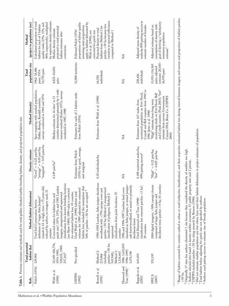
Table

1.Previousestimates

andmethodsusedfortotalgolden-cheeked

warblerbreedinghabitat,density,andprojected

populationsize.

Refs.

Totalpotential

habitat

(ha)

Method(habitat

delineation)

Den

sity

estimate

Method(den

sity)

Total

populationsize

Method

(project

topopulationsize)

Pulich

(1976)

129,904

UsedSoilConservationService

definitionof‘‘virginAsheJuniper’’

(stands6–12m

high,trees>75yearsold),

reducedbyauthor;noim

ageryused;31

counties

‘‘Good’’¼

0.125

pair/ha;

‘‘average’’¼

0.05pair/ha;

‘‘marginal’’¼

0.03pairs/ha

Spot-mappingwithmarked

pop

ulation;

Dallas,Bosque,Kendallcounties;

surveysconducted

in1962and1974

1962:

18,486

pairs;1974:

14,750pairs

Calculatedproportionoftotal

habitat

foreach

of3habitat

qualityranks(23%,31%,and

46%,respectively),multiplied

byrespective

density

estimates

Wahlet

al.

(1990)

32,149–106,776,

1974–1981;

338,035,1989:

237,163a

Correctedvalues

forhabitat

lossand

patch

size

a ;1974,1976,

and1981Landsat

imagery,unsupervisedandsupervised

classificationfrom

know

nbreedinglocations

(see

Shaw

1989);1989valueiscorrected

forestimated

habitat

loss;43counties

0.149

pair/hab

Medianestimatefor16sitescin

11

counties

determined

primarilyby1-m

ile

transect

method(E

mlen1971);surveys

conducted

in1987,

1988

4,822–16,016

pairs

Mediandensity

estimate

projected

tototalpotential

habitat

estimates

after

corrections

USFW

S(1992)

Notspecified

UsedW

ahlet

al.(1990)

habitat

total

estimatefor1989adjusted

forestimated

habitat

loss;included

theassumptionthat

34%

ofpatches<50haareoccupied

d

Estim

ates

from

Pulich

(1976)forgood,average,

andmarginal

Estim

ates

foreach

of3habitat

ranks

from

Pulich

(1976)

13,800territories

Follow

edPulich

(1976)

proportionsofhabitat

quality

assumingsameproportions

applyto

habitat

delineatedby

Wahlet

al.(1990);not

correctedforpatch

size

Rowellet

al.

(1995)

Method2:

215,066

(including

patches<50ha:

545,948);

Method1:

1,116,665

1990–1992Landsat,Ashejuniper-deciduous

woodlandswith>75%

canop

ycoverand

patches>50ha;Method1:unsupervised

classificationofpolygons;Method2:

supervised

classificationfrom

pointlocations;35

counties

0.30individuals/ha

Estim

ates

from

Wahlet

al.(1990)

64,520

individuals

Projected

density

tototal

habitat

from

Method2for

patches>50habecause

less

variationin

spectralreflectance

compared

toMethod1

Diamondand

True(1998)

e1986:

1,652,035

1996–1997:

1,676,140

1986and1996–1997

Landsat;landcover

classified

asAshejuniper,ormixed

juniper-

oak

forest/w

oodland,ormixed

orprimarily

deciduousforest

NA

NA

NA

NA

Rappoleet

al.

(2003)

643,454

UsedDiamondandTrue(1998)

classificationbutremovedpatches<5haf;

29counties

0.188

territorialmales/ha;

89%

pairingsuccessg

Estim

ates

from

167males

from

monitoredpopulationonFortHood,

CoryellandBellcounties

from

1992to

1996(Jette

etal.1998)

228,426

individuals

Adjusted

meandensity

of

malesby89%pairingsuccessto

estimatenumber

offemales

SW

CA

(2007)

552,195

2004digitalim

agery;>50%

canopyclosure

composed

oflargeAshejuniper

and

deciduoustrees;patches>4ha;43counties

‘‘High’’¼

0.22pair/ha;

‘‘low’’¼

0.025pair/ha

‘‘High’’estimatefrom

long-term

monitoringstudyonFortHood,Bell

andCoryellcounties

(Peak2003);‘‘low’’

estimatefrom

surveysGovernment

CanyonSNA,Bexar

Co.(U

SFW

S2004)

13,931–116,565

pairs;adjusted

estimate:20,445–

26,978pairs

Adjusted

estimatebased

on

assumptionsofdensity

with

goalofderivinga‘‘satisfactory

minim

um

population

estimate’’

aRange

ofhabitat

correctedforcounties

ranked

asurban

orrural(subjectiveclassification),andtheirrespective

estimated

habitat

loss

duringintervalbetweenim

ageryandsurveysandproportionofhabitat

patches

>50ha.

bOriginally

17sitesbutauthors

elim

inated

1site

because

they

considered

thedensity

ofwarblers

toohigh.

cAuthors

selected

sitesbased

onknow

nwarbleroccurrence;15publicproperty

sitesand2private.

dUSFW

Sincluded

patches<50hacitingresearch

byBenson(1990).

eDid

notestimatewarblerpopulationsize

butothershaveusedtheirhabitat

delineationto

project

estimates

ofpop

ulation.

fTotalhabitat

before

adjustingforpatch

size

notspecified

byauthors.

gAuthors

usedpairingsuccessto

estimatesize

offemalepopulation.

Mathewson et al. �Warbler Population Abundance 3

of 6 surveys (3 double-observer surveys) to determine warblerpresence (Collier et al. 2010). We surveyed 434 patches forwarbler presence in 2008 and 2009 and if we detected awarbler during occupancy surveys, we returned to the patchto conduct abundance surveys (see below).To select patches for occupancy surveys, we stratified

patches based on administrative units defined by USFWS(USFWS 1992) and used a probability proportional to size(PPS) sampling design (Thompson 2002a), in which werandomly selected habitat patches proportional to the distri-bution of patch sizes across the range. Because habitatpatches often spanned multiple public and private land-owners, we attempted to locate and contact all propertyowners of randomly selected patches. However, our accessto the entirety of each patch was sometimes limited becauseof inability to locate landowners, lack of response, unwill-ingness to participate by landowners, or other logisticalconstraints. Because landowners tend to base their partici-pation on multiple factors that are often not associated withland management practices that would influence warblerabundance (Hilty and Merenlender 2003, DeBoer andDiamond 2006, Sorice et al. 2011), we assumed that suchaccess restrictions did not bias our sampling. Furthermore,we assumed that properties for which we were unable toacquire access were missing from our sample completely atrandom (Stevens and Jensen 2007). We did not stratify byownership type so we focused considerable effort on acquir-

ing access to private property. Our approach further assumedthat variability in habitat conditions was not related consis-tently to designation as private versus public lands as fewpublic or private properties are managed specifically forwarbler habitat in Texas (Groce et al. 2010).

Abundance Surveys

Within each patch selected for abundance surveys, we buff-ered each survey patch to reduce the proportion of survey areathat would fall outside of a habitat patch, such that pointcount centers in patches >40 ha were located �100 m fromthe edge and points in patches�40 ha were�25 m from theedge. Under those constraints, we randomly established themaximum number of point count stations while ensuring a400-mminimum distance between point count centers usingArcGIS 9.3. Small patches (<10 ha) that were inadvertentlyskipped because they violated the 400-m spacing constraintwere processed a second time without the spacing constraintto ensure adequate coverage of point survey locations withinsmall patches. Given our spacing and random placement, weassumed abundance counts at each point were independentwithin patches. Because our sampling unit was the patch, wedid not incorporate any within-patch habitat variability thatcould influence local differences in male density. We as-sumed that our random distribution of point count stationscaptured any within-patch habitat heterogeneity in localvegetation or densities.

Figure 1. Distribution of mixed woodland patches, and locations of abundance surveys conducted during 2008 and 2009 on private or public lands in the 35county breeding range of the golden-cheeked warbler in Texas, USA.

4 The Journal of Wildlife Management

Patches selected for point count surveys were conditionalon positive detections of warblers during occupancy surveys,but we conducted point count surveys independent of theoccupancy sampling process. As such, a zero patch-levelabundance estimate was a recordable result when we detectedno warblers during point count surveys. During mid-Marchto mid-May 2008 and 2009, we conducted abundance sur-veys for warblers using 100-m fixed-radius point countsfollowing methods detailed by Laake et al. (2011).Surveys began at sunrise and ended no later than 13:00.When surveyors detected a bird during occupancy surveys,they immediately initiated point count surveys at the pre-determined point count locations. However, if sufficient timewas not available to conduct the surveys within the same day,we returned within a week of the occupancy survey. We useda dependent double-observer sampling approach (Cook andJacobson 1979, Nichols et al. 2000). At each survey point, werandomly assigned primary or secondary observer status.During the 5-minute survey, the primary observer commu-nicated visual and auditory detections of male warblers to thesecondary observer, noting the direction and classifying theapproximate distance into a distance bin (0–50 m or 50–100 m). Concurrently, the secondary observer recordeddetections of any individuals missed by the primary observer(Laake et al. 2011). The combined data from the primary andsecondary observers represents a 2-sample capture history.To maximize the spatial distribution of sample locations, wevisited each patch on 1 occasion for abundance surveys(Thompson 2002b).We did not conduct point counts duringinclement weather or periods of high wind. We followed thestandard assumptions for point count surveys: 1) populationclosure, 2) observers correctly identified birds, 3) no doublecounting, and 4) observers correctly estimated distances tobirds (Buckland 2006, Johnson 2008).

Analysis

Tomodel male warbler abundance across the breeding range,we first estimated observed patch-specific density using ourpoint count survey data. Next, using an information-theo-retic approach to select the best fitting model given the data(Burnham and Anderson 2002); we regressed patch-specificpredictor variables against the observed patch-specific den-sity estimates and developed a predictive equation relatingbiological metrics to density at the patch scale. Using thepredictive equation, we predicted densities (as well as lowerand upper 95% CL) for each patch of potential habitat fromour delineation across the range and converted those topatch-specific abundance. Finally, we used a Monte Carlosimulation to randomly identify occupied patches based ontheir predicted occupancy probability (Collier et al. 2012)and summed the resultant abundance estimates for eachrandomly selected patch to generate a population abundanceestimate with lower and upper 95% confidence limits for each1,000 realizations.We combined point count data collected during 2008

and 2009 because we independently selected point countlocations for each study year and we assumed minimal annualvariation of patch-level warbler densities. We examined our

assumption using the patches randomly selected for abun-dance surveys in both study years. We estimated observedpatch-specific density using the count of male warblers stan-dardized to the total surveyed area (i.e., 3.14 ha for 100-mfixed-radius sample area) within each patch. We assumedthat the effect of 100-m radius point count locations thatincluded non-woodland vegetation based on our patch de-lineation was minimal. We used counts of abundance un-corrected for detection probability because a preliminaryevaluation revealed estimated double observer detection ratesfor warblers using our survey design were high (probability ofdetection ¼ 0.97; Laake et al. 2011). Furthermore, our un-corrected density estimates will be comparable to previousresearch on warbler densities and abundance that have notincluded detection corrections in their estimates (Table 1).We acknowledge that by implicitly assuming a detectionprobability of 1.0 we likely underestimated density; thus,our estimates may be conservative (Pollock et al. 2002,Thompson 2002b). We assumed that density was constantacross patches and that the random distribution of oursampling points captured any within-patch vegetationheterogeneity.To evaluate the relationships between observed density of

male warblers and our predictor variables, we used general-ized linear modeling (GLM) with a negative binomial dis-tribution of the raw count data (McCullagh and Nelder1989, White and Bennets 1996). We included total areasurveyed at the patch scale as an offset term to standardizeour count data to a density estimate for comparison acrosspatches. We used a negative binomial distribution of ourcount data instead of the Poisson distribution commonlyused for count data because the negative binomial provides aflexible approach to addressing overdispersion (White andBennets 1996).We assembled 8 competing models (Table 2) for predicting

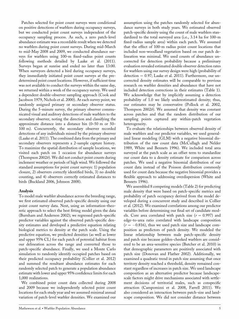
male density that were based on patch-specific metrics andprobability of patch occupancy derived from the model de-veloped during a concurrent study and described in Collieret al. (2012). We examined correlations among our predictorvariables before determining our final set of candidate mod-els. Core area correlated with patch size (r ¼ 0.997) andedge-to-area ratio correlated with landscape composition(r ¼ �0.816), thus we used patch size and landscape com-position as predictors of patch density. We modeled thelinear relationship between male patch-specific densityand patch size because golden-cheeked warblers are consid-ered to be an area-sensitive species (Butcher et al. 2010) inthat demographic parameters are positively associated withpatch size (Donovan and Flather 2002). Additionally, weexamined a quadratic trend in patch size assuming that onceterritory density reached a threshold, density remained con-stant regardless of increases in patch size. We used landscapecomposition as an alternative predictor because landscape-scale factors might drive mechanisms associated with settle-ment decisions of territorial males, such as conspecificattraction (Campomizzi et al. 2008, Farrell 2011). Wealso considered an interaction between patch-size and land-scape composition. We did not consider distance between

Mathewson et al. �Warbler Population Abundance 5

patches because our landscape composition metric capturedthis variability and previous research on warbler occurrenceat the point-scale indicated that these variables were notas predictive as is landscape composition (DeBoer andDiamond 2006, Magness et al. 2006).We also used the patch occupancy prediction from Collier

et al. (2012) as a predictor variable of abundance. The geo-additive semiparametric approach detailed in Collier et al.(2012) predicted occupancy probability (ci) as a function ofcovariate data (patch size and landscape composition) andspatial location within the warbler’s range expressed as

logitðciÞ ¼ b0 þ blXl þX20

k¼1ukðLocationi � kkÞ þ "i

where the bl Xl represents a vector of l predictor variables(patch size, landscape composition, patch size-landscapecomposition interaction, and patch-specific UniversalTransverseMercator [UTM] coordinates) entering the mod-el linearly and ðLocation� kkÞ represents the effect of spatiallocation for each surveyed habitat patch (Gimenez et al.2009). Collier et al. (2012) used a temporal covariate rep-resenting sample survey date for detection modeling becausedate of survey has been shown to adequately predict detectionrates of warblers at the patch scale (Collier et al. 2010).We used an information-theoretic approach (Burnham and

Anderson 2002) to evaluate competing models. We rankedmodels using Akaike’s Information Criterion (AICc) cor-rected for small sample sizes. We calculated Akaike weights(wi) to indicate relative likelihood of each model as the bestapproximating model given the data for our set of candidatemodels. We considered models �4 DAIC units to be com-petitive. We judged model adequacy by performing a 10-foldcross-validation. We performed a likelihood ratio test of asaturated model that included occupancy and an interactionbetween patch size and landscape composition compared to aconstant model to examine over-dispersion (Venables andRipley 2002).We used the best fitting model given our model set and

predicted patch-specific density of male warblers for eachhabitat patch that we delineated across the range

(n ¼ 63,616 patches). We converted predicted density topredicted patch-specific abundance and ran Monte Carlosimulations using the equation

N ¼Xn

i¼1ðyi � area� kiÞ

where yi is the predicted patch-specific density estimate andarea (ha) is the size of each patch. The covariate k representeda random assignment of occupancy (0 or 1) based on randomdraws from a Bernoulli distribution using the predicted patchoccupancy rates from Collier et al. (2012). We generated adistribution of abundance estimates and associated upper andlower bounds using 1,000 replicates of the above simulationwhere the summed abundance values for those patches wherek ¼ 1 represented the predicted population.When surveying avian species, counting a single bird mul-

tiple times is possible, which would bias point survey data(Buckland 2006). Given our short point count period(5 min), we concluded that double counting was unlikely;however, we were interested in exploring the potentialimpacts of being wrong in reaching such a conclusion.Thus, we estimated minimum density and population sizebased on 2 possible scenarios of double counting. First, giventhat double counting could not occur if observers detected 0or 1 warbler at a point during a survey, and that the likelihoodof observers having over counted when reporting 2 birds isunlikely given our survey design, we re-examined our data bylimiting total counts at a point to a maximum of 2 (Table 3).Second, to exclude potential bias of double counting warblersbetween the 2 observers, we used the number of birdscounted only by the primary observer, representing the min-imum count that would be obtained from a single-visitstandard point count (Nichols et al. 2000).

RESULTS

Abundance Counts and Density EstimationWe conducted 1,057 point count surveys in 301 mixedwoodland patches (2008: n ¼ 151 patches; 2009: n ¼ 150)across the warbler’s breeding range (Fig. 1). Survey points per

Table 2. Model selection statistics formodels using negative binomial regression explaining patch-specific density of golden-cheekedwarblers in Texas, in 2008and 2009.

Modelsa Kb Log likelihood AICcc DAICc

d wie

Occ 2 �515.78 1035.57 0 0.799Size þ LS 3 �516.86 1039.71 4.20 0.098Size � LS 4 �516.10 1040.20 4.75 0.074Size2 3 �518.47 1042.94 7.43 0.019logSize 2 �520.30 1044.60 9.04 0.009LS 2 �522.87 1049.74 14.17 0.001Size 2 �522.92 1049.85 14.28 0.001Null 1 �535.35 1072.71 37.10 0.000

a Occ ¼ estimated occupancy from semiparametric model of Collier et al. (2012), Size ¼ size of habitat patch (ha), Size2 ¼ size of habitat patch quadratictrend, LS ¼ landscape composition.

b K ¼ no. of parameters.c AICc ¼ Akaike’s Information Criterion corrected for small sample sizes.d DAICc ¼ AICc relative to the most parsimonious model.e wi ¼ AICc model weight.

6 The Journal of Wildlife Management

patch ranged from 1 to 35 (mean ¼ 3.5, SD ¼ 4.11). Wedetected 796 warblers during both years of our surveys. Forpatches surveyed for abundance estimation, patch size rangedfrom 2.8 to 26,967 ha (mean ¼ 743.7, 95% CI ¼ 497.2–990.2, median ¼ 141.2, n ¼ 301). Mean patch size forpatches primarily in private ownership ranged from 3.2 to26,970 ha (mean ¼ 740.1, 95% CI ¼ 388.3–1,093.5,median ¼ 147.3, n ¼ 178) and for public properties rangedfrom 2.8 to 11,880 ha (mean ¼ 747.8, 95% CI ¼ 420.3–1,075, median ¼ 119.2, n ¼ 123). Mean landscape compo-sition (% woodland vegetation within 400-m radius) rangedfrom 15% to 92% (mean ¼ 65.4, 95% CI ¼ 63.7–67.0,median ¼ 67.1, n ¼ 301). Mean landscape compositionfor patches primarily in private ownership ranged from15% to 91% (mean ¼ 64, 95%CI ¼ 62–66, median ¼ 65.7,n ¼ 178) and for public properties ranged from 26% to 92%(mean ¼ 67.2, 95% CI ¼ 64.3–70.1, median ¼ 72.8,n ¼ 123). For the sub-sample of patches surveyed in bothyears (n ¼ 34), density estimates were similar (2008:0.25 males/ha, 95% CI ¼ 0.18–0.32; 2009: 0.23 males/ha,95% CI ¼ 0.15–0.29), supporting our assumption of mini-mal annual variation between our survey years.Thirty-four percent (n ¼ 301) of patches in which we

conducted abundance point counts had no warbler detec-tions. Mean observed patch-specific density of male warblersfor both years, was 0.23 males/ha (95% CI ¼ 0.197–0.252,n ¼ 301 patches). Density varied between USFWS recoveryregions (USFWS 1992); mean observed density in the northregion was 0.15 males/ha (95% CI ¼ 0.10–0.17, n ¼ 86patches), the central region equaled 0.19 males/ha (95%CI ¼ 0.15–23, n ¼ 106), and the south region equaled0.32 males/ha (95% CI ¼ 0.26–37, n ¼ 109).

Model Results and Abundance Estimation

The goodness-of-fit test indicated that the saturated modelfit the data (x24 ¼ 52.1, P < 0.001). Based on our modelselection results, patch-specific occupancy probability bestpredicted male warbler density (Table 2). The standardizedmodel parameter estimates for the fitted model indicated thatfor every 0.25 increase in predicted patch occupancy proba-bility (i.e., 1-unit increase for scaled data), the density ofmales increased by 61% (b ¼ 0.478, 95% CI: 0.326–0.636).Using our predicted patch-specific density estimates as a

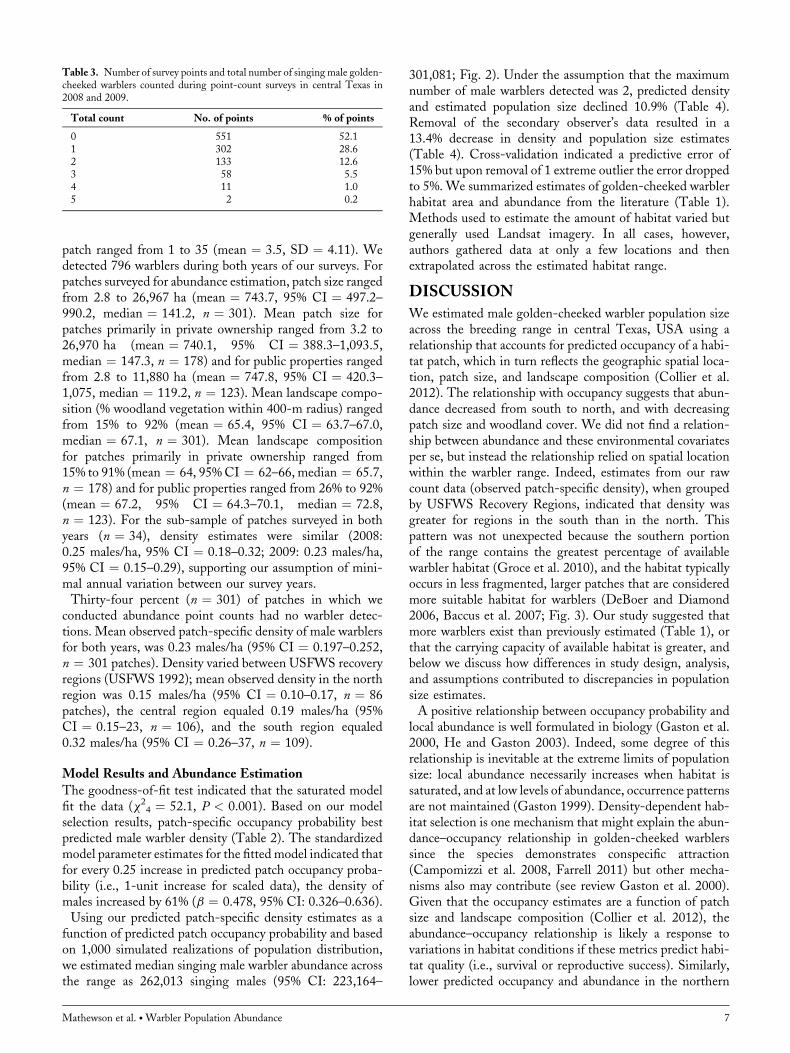
function of predicted patch occupancy probability and basedon 1,000 simulated realizations of population distribution,we estimated median singing male warbler abundance acrossthe range as 262,013 singing males (95% CI: 223,164–

301,081; Fig. 2). Under the assumption that the maximumnumber of male warblers detected was 2, predicted densityand estimated population size declined 10.9% (Table 4).Removal of the secondary observer’s data resulted in a13.4% decrease in density and population size estimates(Table 4). Cross-validation indicated a predictive error of15% but upon removal of 1 extreme outlier the error droppedto 5%. We summarized estimates of golden-cheeked warblerhabitat area and abundance from the literature (Table 1).Methods used to estimate the amount of habitat varied butgenerally used Landsat imagery. In all cases, however,authors gathered data at only a few locations and thenextrapolated across the estimated habitat range.

DISCUSSION

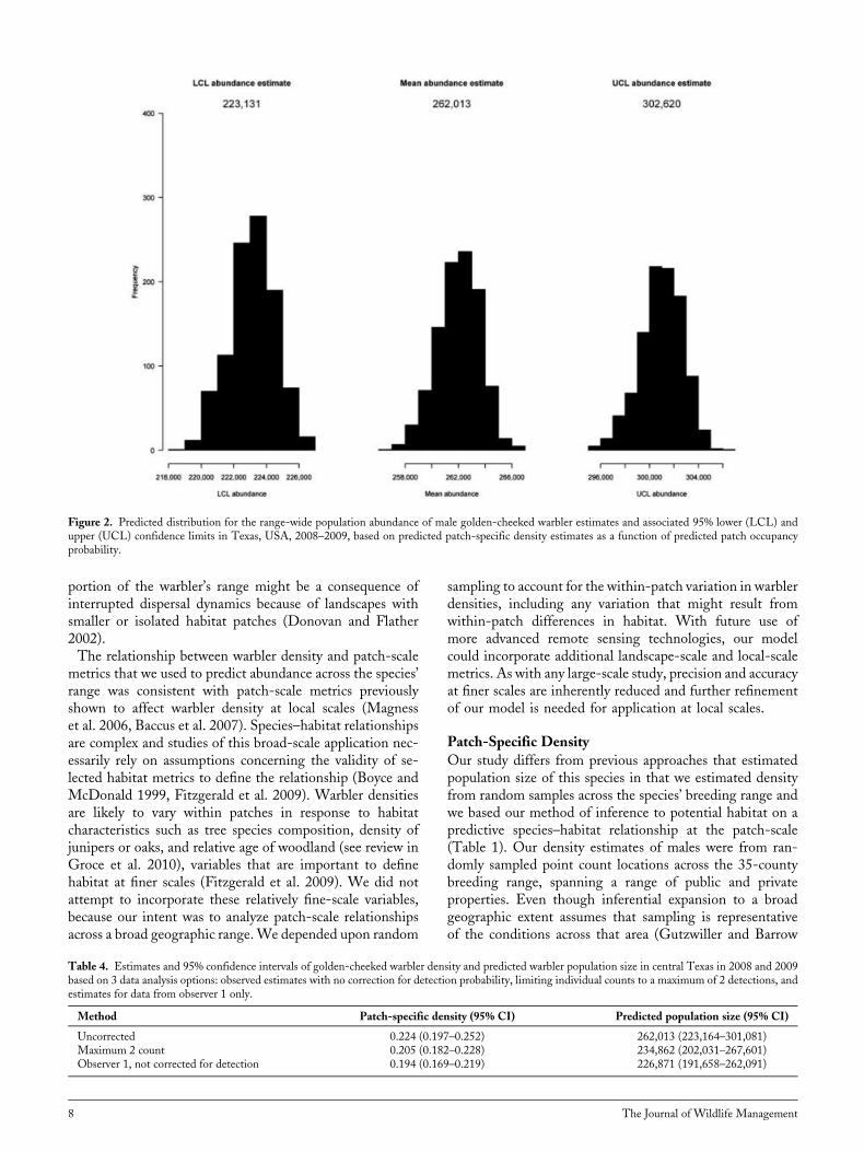
We estimated male golden-cheeked warbler population sizeacross the breeding range in central Texas, USA using arelationship that accounts for predicted occupancy of a habi-tat patch, which in turn reflects the geographic spatial loca-tion, patch size, and landscape composition (Collier et al.2012). The relationship with occupancy suggests that abun-dance decreased from south to north, and with decreasingpatch size and woodland cover. We did not find a relation-ship between abundance and these environmental covariatesper se, but instead the relationship relied on spatial locationwithin the warbler range. Indeed, estimates from our rawcount data (observed patch-specific density), when groupedby USFWS Recovery Regions, indicated that density wasgreater for regions in the south than in the north. Thispattern was not unexpected because the southern portionof the range contains the greatest percentage of availablewarbler habitat (Groce et al. 2010), and the habitat typicallyoccurs in less fragmented, larger patches that are consideredmore suitable habitat for warblers (DeBoer and Diamond2006, Baccus et al. 2007; Fig. 3). Our study suggested thatmore warblers exist than previously estimated (Table 1), orthat the carrying capacity of available habitat is greater, andbelow we discuss how differences in study design, analysis,and assumptions contributed to discrepancies in populationsize estimates.A positive relationship between occupancy probability and

local abundance is well formulated in biology (Gaston et al.2000, He and Gaston 2003). Indeed, some degree of thisrelationship is inevitable at the extreme limits of populationsize: local abundance necessarily increases when habitat issaturated, and at low levels of abundance, occurrence patternsare not maintained (Gaston 1999). Density-dependent hab-itat selection is one mechanism that might explain the abun-dance–occupancy relationship in golden-cheeked warblerssince the species demonstrates conspecific attraction(Campomizzi et al. 2008, Farrell 2011) but other mecha-nisms also may contribute (see review Gaston et al. 2000).Given that the occupancy estimates are a function of patchsize and landscape composition (Collier et al. 2012), theabundance–occupancy relationship is likely a response tovariations in habitat conditions if these metrics predict habi-tat quality (i.e., survival or reproductive success). Similarly,lower predicted occupancy and abundance in the northern

Table 3. Number of survey points and total number of singingmale golden-cheeked warblers counted during point-count surveys in central Texas in2008 and 2009.

Total count No. of points % of points

0 551 52.11 302 28.62 133 12.63 58 5.54 11 1.05 2 0.2

Mathewson et al. �Warbler Population Abundance 7

portion of the warbler’s range might be a consequence ofinterrupted dispersal dynamics because of landscapes withsmaller or isolated habitat patches (Donovan and Flather2002).The relationship between warbler density and patch-scale

metrics that we used to predict abundance across the species’range was consistent with patch-scale metrics previouslyshown to affect warbler density at local scales (Magnesset al. 2006, Baccus et al. 2007). Species–habitat relationshipsare complex and studies of this broad-scale application nec-essarily rely on assumptions concerning the validity of se-lected habitat metrics to define the relationship (Boyce andMcDonald 1999, Fitzgerald et al. 2009). Warbler densitiesare likely to vary within patches in response to habitatcharacteristics such as tree species composition, density ofjunipers or oaks, and relative age of woodland (see review inGroce et al. 2010), variables that are important to definehabitat at finer scales (Fitzgerald et al. 2009). We did notattempt to incorporate these relatively fine-scale variables,because our intent was to analyze patch-scale relationshipsacross a broad geographic range.We depended upon random

sampling to account for the within-patch variation in warblerdensities, including any variation that might result fromwithin-patch differences in habitat. With future use ofmore advanced remote sensing technologies, our modelcould incorporate additional landscape-scale and local-scalemetrics. As with any large-scale study, precision and accuracyat finer scales are inherently reduced and further refinementof our model is needed for application at local scales.

Patch-Specific Density

Our study differs from previous approaches that estimatedpopulation size of this species in that we estimated densityfrom random samples across the species’ breeding range andwe based our method of inference to potential habitat on apredictive species–habitat relationship at the patch-scale(Table 1). Our density estimates of males were from ran-domly sampled point count locations across the 35-countybreeding range, spanning a range of public and privateproperties. Even though inferential expansion to a broadgeographic extent assumes that sampling is representativeof the conditions across that area (Gutzwiller and Barrow

Table 4. Estimates and 95% confidence intervals of golden-cheeked warbler density and predicted warbler population size in central Texas in 2008 and 2009based on 3 data analysis options: observed estimates with no correction for detection probability, limiting individual counts to a maximum of 2 detections, andestimates for data from observer 1 only.

Method Patch-specific density (95% CI) Predicted population size (95% CI)

Uncorrected 0.224 (0.197–0.252) 262,013 (223,164–301,081)Maximum 2 count 0.205 (0.182–0.228) 234,862 (202,031–267,601)Observer 1, not corrected for detection 0.194 (0.169–0.219) 226,871 (191,658–262,091)

Figure 2. Predicted distribution for the range-wide population abundance of male golden-cheeked warbler estimates and associated 95% lower (LCL) andupper (UCL) confidence limits in Texas, USA, 2008–2009, based on predicted patch-specific density estimates as a function of predicted patch occupancyprobability.

8 The Journal of Wildlife Management

2001) no previous study reporting population sizes of gold-en-cheeked warblers has used density estimates from ran-domly located study sites. Previous calculations of warblerabundance used density estimates primarily from study sitesin the north or central portions of the breeding range (e.g.,Pulich 1976, Rappole et al. 2003). Furthermore, some pop-ulation size estimates were based on a mean or mediandensity estimate from a few locations (Wahl et al. 1990,Rowell et al. 1995, Rappole et al. 2003), implying a constantdensity and thus failing to address variation in densitiesamong habitat patches and across the range (Royle andNichols 2003). Although Wahl et al. (1990) estimatedsite-specific densities at 17 sites in 11 counties, they didnot incorporate variation in abundance in their populationsize estimate because they used the median density estimate,assuming constant density across the range. Pulich (1976)addressed regional variation in density by deriving estimatesfrom 3 study sites across the range; however, for projection topotential habitat he assumed a constant density within 3habitat assessment ranks (Table 1). We addressed regionaland among-patch heterogeneity in density by defining habi-tat patches as our sampling unit and projecting patch-specific

densities to our potential habitat delineation. Although ourapproach requires the assumption of constant density withinpatches, we suggest that this is an improvement from previ-ous estimates of golden-cheeked warbler abundance.We used standard methods for avian point count surveys

and we assumed a detection probability of 1.0. It is widelyrecognized that assuming a constant detection probabilityresults in biased estimates because failing to account fordetection typically produces underestimates of abundance(Pollock et al. 2002, Thompson 2002b, Johnson 2008).We accepted the potential for a negative bias because evi-dence that the use of a dependent double-observer closecapture model resulted in a high probability (>0.97) ofdetecting a male warbler by at least 1 of the 2 observers(Laake et al. 2011). Multiple factors influence detectability,including skills of observers, habitat, ambient noise, weather,distance, and temporal effects (Johnson 2008). Correctingfor detectability requires additional assumptions concerningthese sources of heterogeneity in detection.Johnson (2008) warned against making additional assump-

tions concerning detection heterogeneity until further inves-tigations identify these sources because it could result in the

Figure 3. Predicted patch-specific occupancy probability for male golden-cheeked warblers in Texas, USA, 2008–2009. Figure from Collier et al. (2012).

Mathewson et al. �Warbler Population Abundance 9

application of an inadequate correction factor and, subse-quently, a false confidence in accuracy. Several factors incombination likely affected detectability of warblers differ-ently across the range in this study and by not systematicallycorrecting for detection we eliminated any concerns regard-ing which sources of variability should be controlled statisti-cally (Diefenbach et al. 2007, Johnson 2008). However, wecollected our data in a manner conducive to future evaluationof some these effects on detection heterogeneity. For exam-ple, the assumption of constant detection could be relaxed byapplying a distance-based or double-observer approach toour data (Nichols et al. 2000, Laake et al. 2011). We furtheraccepted the potential for negative bias from our uncorrecteddensity estimates to produce more conservative estimatesgiven the endangered status of the warbler.We attempted to reduce variation in detectability and to

minimize bias associated with standard avian point countsthrough our study design (Pollock et al. 2002, Johnson2008). We used 5-minute point count periods to minimizedouble counting of birds within the survey area or by count-ing birds that have moved through the area (Buckland 2006).We used a dependent double-observer method because it isrobust to violations of the closure assumption (Moore et al.2004). Although we consistently use well-trained observers,another benefit of the double-observer approach is that itreduces the prospect of species misidentification (Mooreet al. 2004). We assumed a closed population because weconducted single-occasion point counts in each patch. Giventhe distribution of our survey patches, individuals did notlikely move among our survey patches. By conducting single-occasion point counts, we were unable to detect and controlfor any temporal variation, but this was a trade-off to increaseour survey efforts across a greater spatial extent (Thompsonet al. 2002). To minimize temporal variation, we limited oursurveys to the peak of the warbler breeding season, but werecognize that detection probability decreases across thisperiod and we likely negative biased counts as the seasonprogressed (Collier et al. 2010).We report an estimate of the population size of male

warblers during the breeding season, making no assumptionsregarding breeding status of males. In other words, ourcounts included males that were territorial and paired, terri-torial and unpaired, or non-territorial floaters. Previous stud-ies have reported population sizes of total breedingindividuals that required assumptions associated with popu-lation-level pairing success to obtain an estimate of femalepopulation size (Table 1). The bias associated with assump-tions of male breeding status, and consequently pairingsuccess, depends on the study design, survey or monitoringeffort, or adjustments to male-based detections. Becausemany songbird populations, including the golden-cheekedwarbler, consist of territorial but unpaired males (Newton1992), assuming that each male detected during a surveyrepresents a breeding pair overestimates the female propor-tion of the population. Nevertheless, even with informationgarnered from monitoring protocols concerning pairing suc-cess, these studies tend to overlook non-territorial males thatcan constitute a substantial proportion of a population. For

many songbirds, particularly those in fragmented habitats,male breeding status varies with habitat condition and de-mographic factors, such as densities or age structure (Newton1992, Jette et al. 1998, Bayne and Hobson 2001). Althoughstudies that monitor territories can capture variability in malebreeding status at a local scale, these methods are impracticalfor broad-scale application (Buckland 2006). Until furtherassessment of how male breeding success varies across therange, we are unable to determine the degree of precision andbias in reported population sizes adjusted by pairing successestimates from a few locations. In our study, we eliminatedthe need for uninformed adjustments to calculate femalepopulation size and instead we present an approach thatcan incorporate future consideration of male breeding statusacross the range.

Other Habitat Delineations

Population size estimates necessarily depend on the habitatdelineation used to project a local density estimate to therange of potential habitat. Thus, the underlying question ofall attempts to estimate population size is how habitat isdefined and what habitat characteristics can be estimatedusing remotely sensed techniques. Much of the variation inestimated population sizes for the golden-cheeked warblerare created because of differences in data sources used toidentify potential habitat (e.g., Landsat imagery, NLCD),each having differing resolutions and classification accuracies(Table 1). In addition, studies use different characterizationsof the landscape to define habitat, oftentimes assuming aminimum threshold for warbler occurrence or other restric-tions based on evaluations of habitat quality (Table 1). Theseapproaches are inherently conservative, producing negativelybiased habitat and population size estimates. Given theuncertainties in identifying warbler habitat in terms of habi-tat quality, we made no assumption regarding habitat qualityin our broadly defined habitat delineation and provided anestimate of available potential habitat. Indeed, our totalhabitat estimate is similar to other recent studies whenassumptions regarding habitat quality are removed(Diamond and True 1998, Diamond 2007). There may beconcern that overestimating habitat would inflate our popu-lation size estimates, but the additional woodland included inour liberal estimation of habitat was primarily small patchesand edge habitat (Fig. 3; Morrison et al. 2010, Collier et al.2012). Occupancy probability was �0.10 for 59% of thepatches in our habitat delineation (Collier et al. 2012) result-ing in low predicted density estimates for a large portion ofthe habitat; thus, including habitat often assumed as lowerquality contributed little to our total population sizeestimates.Previous population size estimates are from data acquired

on primarily public properties, whereas over half of thehabitat patches in our study were private properties acrossthe warbler’s range. Given the differences in land uses ob-served on our private properties and that there was nosignificant difference in our habitat metrics between privateand public lands, we assumed that warbler density andhabitat conditions did not vary from properties for which

10 The Journal of Wildlife Management

we did not acquire access. Similarly, habitat patches withinwhich landowners actively managed for golden-cheekedwarblers did not bias our sample of public properties. Ofpublic lands, TPWD state parks dominated our sample andfew of these implement management plans for warblers(Groce et al. 2010). Only 5% of our survey patches wereon properties managed specifically for warblers (e.g.,Balcones Canyonland Preserve, Travis County).Our study is an example of how researchers and land

managers can use predictive models to estimate populationabundance. Application of this model is at the range-widescale but implementation of our approach at the regionalscale is possible by incorporating additional information torefine abundance relationships. As remote-sensing technol-ogy evolves, we can examine additional habitat variables thatmight inform within-patch heterogeneity. Furthermore, ourframework provides the opportunity to include detectionprobability to move beyond an index of warbler abundance(Johnson 2008).

MANAGEMENT IMPLICATIONS

Our results indicate that warblers were more abundant inlarger woodland patches of which most occur in the southernportion of the breeding range. Having this knowledge willhelp direct limited resources to the most effective areas forconservation of the species and will help guide managementdecisions (Fitzgerald et al. 2009). The population abundanceestimate we generated can also inform recovery planning forthe warbler. A better understanding of the influence of patchsize and landscape composition on the occupancy and abun-dance of golden-cheeked warblers will provide a tool forrecovery planning. If recovery planning is to involve thedesignation of focal areas for prioritizing conservationefforts, then the model developed here could provide avaluable planning aid in the process. As future habitat con-servation plans and biological assessments are developed, theresults of this work could inform impact assessments forestimating incidental take as well as supporting the develop-ment of more accurate metrics for crediting and mitigationprograms. By providing a framework for more reliably pre-dicting abundance and changes in abundance, our resultsprovide the basis for assessment of this species’ status. Withfurther refinement of the model to account for differences inwithin-patch habitat quality, our results form the basis foradvancing a system for monitoring of the warbler’s abun-dance patterns, ultimately supporting decisions leading torecovery.

ACKNOWLEDGMENTS

The Texas Department of Transportation provided supportfor our work. Additionally, we acknowledge Texas Parks andWildlife Department (TPWD) for support. We appreciatethe private landowners who graciously allowed us access totheir property, as well as TPWD, the U. S. Fish andWildlifeService, The Nature Conservancy, City of Austin, TravisCounty, and the Lower Colorado River Authority. Wethank J. Dunk, P. Hamel, R. Peak, W. Thogmartin, and

F. Thompson III for helpful discussions regarding our re-search. We also thank J. Sedinger, B. Block, C. Farquhar,D. Wolfe, and numerous anonymous referees for insightfulreviews on previous versions of this manuscript. We grate-fully acknowledge A. Snelgrove, K. Skow, B. Stevener, andA. Dube for logistical support, as well as the many techni-cians and graduate students from Texas A&M University.B. A. Collier acknowledges partial support from Award No.KUS-C1-016-04 given by the King Abdullah University ofScience and Technology (KAUST).

LITERATURE CITEDBaccus, J. T., M. E. Tolle, and J. D. Cornelius. 2007. Response of golden-cheeked warblers (Dendroica chrysoparia) to wildfires at Fort Hood, Texas.Texas Ornithological Society. Occasional Publication 7:1–37.

Bayne, E. M., and K. A. Hobson. 2001. Effects of habitat fragmentation onpairing success of ovenbirds: importance of male age and floater behavior.Auk 118:380–388.

Benson, R. H. 1990. Habitat area requirements of the golden-cheekedwarbler on the Edwards Plateau. Texas Parks and WildfireDepartment, Austin, USA.

Boyce, M. S., and L. L. McDonald. 1999. Relating populations to habitatsusing resource selection functions. Trends in Ecology & Evolution14:268–272.

Buckland, S. T. 2006. Point transect surveys for songbirds: robust method-ologies. Auk 123:345–357.

Burnham, K. P., and D. R. Anderson. 2002. Model selection and multi-model inference: a pratical information-theoretic approach. Springer, NewYork, New York, USA.

Butcher, J. A., M. L. Morrison, D. Ransom, Jr., R. D. Slack, and R. N.Wilkins. 2010. Evidence of a minimum patch size threshold of reproduc-tive success in an endangered songbird. Journal of Wildlife Management74:133–139.

Campbell, S. P., J. A. Clark, L. H. Crampton, A. D. Guerry, L. T. Hatch,P. R. Hosseini, J. J. Lawler, and R. J. O’Connor. 2002. An assessment ofmonitoring efforts in endangered species recovery plans. EcologicalApplications 12:674–681.

Campomizzi, A. J., J. A. Butcher, S. L. Farrell, A. G. Snelgrove, B. A.Collier, K. J. Gutzwiller, M. L. Morrison, and R. N. Wilkins. 2008.Conspecific attractions is a missing component in wildlife habitat model-ing. Journal of Wildlife Management 72:331–336.

Collier, B. A., J. E. Groce, M. L.Morrison, C. Newnam, A. J. Campomizzi,S. L. Farrell, H. A. Mathewson, R. T. Snelgrove, R. J. Carroll, and R. N.Wilkins. 2012. Predicted patch occupancy in fragmented landscapes at therangewide scale for an endangered species: an example of an Americanwarbler. Diversity and Distributions 18:158–167.

Collier, B. A., M. L. Morrison, S. L. Farrell, A. J. Campomizzi, J. A.Butcher, K. B. Hays, D. I. MacKenzie, and R. N. Wilkins. 2010.Monitoring endangered species occupying private lands: case study usingthe golden-cheeked warbler. Journal of Wildlife Management 74:140–147.

Conroy, M. J., J. P. Runge, R. J. Barker, M. R. Schofield, and C. J.Fonnesbeck. 2008. Efficient estimation of abundance for patchily distrib-uted populations via two-phase, adaptive sampling. Ecology 89:3362–3370.

Cook, R. D., and J. O. Jacobson. 1979. A design for estimating visibility biasin aerial surveys. Biometrics 35:735–742.

DeBoer, T. S., and D. D. Diamond. 2006. Predicting presence-absenceof the endangered golden-cheeked warbler (Dendroica chrysoparia).Southwestern Naturalist 51:181–190.

Diamond, D. D. 2007. Range-wide modeling of golden-cheeked warblerhabitat. Project Final Report to Texas Parks & Wildlife, Austin, Texas,USA.

Diamond, D. D., and C. D. True. 1998. Golden-cheeked warbler nestinghabitat area, habitat distribution, and change. Project Final Report toUSFWS, Region 2, Albuquerque, New Mexico, USA.

Diefenbach, D. R., M. R. Marshall, J. A. Mattice, and D. W. Brauning.2007. Incorporating availability for detection in estimates of bird abun-dance. Auk 124:96–106.

Mathewson et al. �Warbler Population Abundance 11

Original Article

Utilization of a Species Occupancy Model forManagement and Conservation

TIFFANY M. MCFARLAND,1 Institute of Renewable Natural Resources, Texas A&M University, College Station, TX 77843, USA

HEATHER A. MATHEWSON, Institute of Renewable Natural Resources, Texas A&M University, College Station, TX 77843, USA

JULIE E. GROCE, Institute of Renewable Natural Resources, Texas A&M University, San Antonio, TX 78215, USA

MICHAEL L. MORRISON, Department of Wildlife and Fisheries Sciences, Texas A&M University, College Station, TX 77843, USA

J. CAL NEWNAM, Texas Department of Transportation, P.O. Box 15426, Austin, TX 78761, USA

R. TODD SNELGROVE, Institute of Renewable Natural Resources, Texas A&M University, College Station, TX 77843, USA

KEVIN L. SKOW, Institute of Renewable Natural Resources, Texas A&M University, College Station, TX 77843, USA

BRET A. COLLIER, Institute of Renewable Natural Resources, Texas A&M University, College Station, TX 77843, USA

R. NEAL WILKINS, Institute of Renewable Natural Resources, Texas A&M University, College Station, TX 77843, USA

ABSTRACT Conserving habitat is increasingly challenging as human populations grow. Remote-sensingtechnology has provided a means to delineate species’ habitat on large spatial scales. However, by combininghabitat delineations with predictions of species’ occurrence, habitat models can provide additional utilityapplications for conservation by allowing us to forecast how changing environmental and landscape con-ditions affect species’ occurrence and distribution.We demonstrate how a spatially explicit habitat occupancymodel for the golden-cheeked warbler (Setophaga chrysoparia) can be used as an impact assessment andconservation planning tool. We used predictions of patch-level occupancy rates and created several scenariosthat simulated the removal or protection of warbler habitats. Resulting changes to habitat structure andavailability were used to assess the resulting impacts of removal or protection on the occurrence probability forremaining habitat patches. By recalculating occupancy based on changes to habitat, our approach provides theability to assess and compare impacts of location and orientation of development so that the least harmfuloption relative to predicted occurrence can be chosen. Potential applications of our modeling approach aremany because our methods provide a useful tool for identifying potential impacts and assisting withmitigation efforts focused on the conservation and management of a species. � 2012 The Wildlife Society.

KEY WORDS conservation planning, golden-cheeked warbler, habitat, landscape management, mitigation, Setophagachrysoparia, species distribution.

Implementation of successful management strategies requireknowledge of animal distribution relative to environmentalconditions and predictions of how animal populations willrespond to direct and indirect environmental impacts(Kantrud and Stewart 1984, Wiens and Rotenberry 1985,Debinski and Brussard 1994, Colwell and Dodd 1995).Spatially explicit habitat models that predict the probabilityof species occurrence on broad spatial scales are useful toolsfor assessing potential impacts of land use or environmentalchanges, or for forecasting the outcome of managementactions (Sagarin et al. 2006, Brotons et al. 2007). For speciesof conservation concern, the implications of habitat loss areoften significant and loss can have long-term implications onpopulation sustainability.The golden-cheeked warbler (Setophaga chrysoparia; here-

after, ‘‘warbler’’) is a Neotropical migratory songbird thatbreeds exclusively in central Texas, USA, in mixed wood-

lands of mature Ashe juniper (Juniperus ashei), oak (Quercusspp.), and other deciduous species (Pulich 1976, Wahl et al.1990). In 1990, the U.S. Fish andWildlife Service (USFWS)listed the warbler as endangered, citing habitat loss andfragmentation as the primary threats to the species(USFWS 1990). Increasing infrastructure development(e.g., roads, utilities) within the warbler’s limited breedingrange creates networks of corridors that can deterioratewoodland habitat due to fragmentation (Peak 2007) andpotentially inhibit exchange and dispersal of individualsbetween patches (Gobeil and Villard 2002, Goodwin andFahrig 2002, Haynes and Cronin 2006, Richard andArmstrong 2010). However, the impacts of environmentalor anthropogenic activities that could fragment potentialhabitat have typically been limited by our knowledge ofthe likelihood of warbler occurrence within those habitats.Any loss of habitat, either from natural phenomena (i.e., fire)or human activities, has the potential to impact the warblerdue to the species’ limited range.Several warbler habitat classifications created in the past

20 years have provided estimates of range-wide habitat

Received: 10 August 2011; Accepted: 14 November 2011

1E-mail: tiffany.mcfarland@agnet.tamu.edu

Wildlife Society Bulletin; DOI: 10.1002/wsb.106

McFarland et al. � Utilization of a Species Occupancy Model 1

distribution (Wahl et al. 1990, Rowell et al. 1995, Rappoleet al. 2003, DeBoer and Diamond 2006, Loomis-Austin,Inc. 2008) based on remotely sensed metrics and researcher-defined descriptions of warbler habitat. Several previoussurveys also evaluated warbler occurrence and habitat asso-ciations, but these studies focused on a few public propertieswith known populations of warblers (Anders and Dearborn2004, Peak 2007, Reidy et al. 2008), reducing the ability ofthe authors to extrapolate avian–habitat relationships acrossthe breeding range. Two studies classified habitat qualityacross the range. DeBoer and Diamond (2006) used sampledata from across the range to model habitat quality.However, their sample size was small (n ¼ 50 patches),and several habitat metrics identified as relevant cannot beassessed remotely and, therefore, cannot be modeled ormapped at the range-wide scale. Diamond (2007) modeledhabitat quality across the range, but estimates of quality werebased on researchers’ evaluation of quality, rather than usingwarbler occurrence data collected in the field to drive thedevelopment of a habitat model.Here we demonstrate how a spatially explicit habitat model

can be utilized as a tool for conservation planning and impactassessment. We used a patch-level habitat occupancy modelfor the warbler built on survey data collected on public andprivate properties across the warbler’s breeding range inTexas (Collier et al. 2012). These patch occupancy predic-tions provided high accuracy in predicting warbler occur-rence at the patch scale and were based on patch size andlandscape composition (hereafter, ‘‘woodland composition’’)metrics combined with a north to south spatial gradient.Unlike previous models, which only delineate potential hab-itat, Collier et al. (2012) can categorize a habitat patch basedon the probability of occupancy and, thus, can be used topredict the impacts of habitat loss or modification on warbleroccupancy, rather than simply calculating the amount ofhabitat change. Herein, we illustrate the use of such a modelby first showing the changes in predicted warbler occupancybased on simulated fragmentation or removal of habitatpatches, and then showing how these effects can provideguidance for warbler conservation and management.Although we were able to sample across the entirety ofthe warbler’s breeding range, occupancy models such asours could also be developed for subsets of the range ofmost species.

METHODS

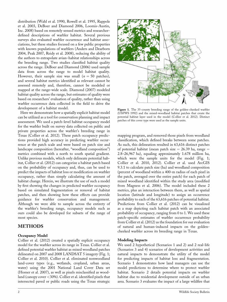
Occupancy ModelCollier et al. (2012) created a spatially explicit occupancymodel for the warbler across its range in Texas. Collier et al.defined potential warbler habitat as mixed woodland patchesdelineated on 2007 and 2008 LANDSAT 5 imagery (Fig. 1;Collier et al. 2010). Collier et al. eliminated nonwoodlandland-cover types (e.g., wetlands, cropland, urban areas,water) using the 2001 National Land Cover Data set(Homer et al. 2007), as well as pixels misclassified as wood-land (canopy cover<30%). Collier et al. identified pixels thatintersected paved or public roads using the Texas strategic

mapping program, and removed those pixels from woodlandclassification, which defined breaks between some patches.As such, this delineation resulted in 63,616 distinct patchesof potential habitat (mean patch size ¼ 26.39 ha, range ¼2.8–26,967 ha), equaling approximately 1.678 million ha,which were the sample units for the model (Fig. 1;Collier et al. 2010, 2012). Collier et al. used ArcGIS9.3.1 to calculate patch size (ha) and woodland composition(percent of woodland within a 400-m radius of each pixel inthe patch, averaged over the entire patch) for each patch ofmixed woodland identified within the study area (modifiedfrom Magness et al. 2006). The model included these 2metrics, plus an interaction between them, as well as spatiallocation (latitude and longitude) to assign an occurrenceprobability to each of the 63,616 patches of potential habitat.Predictions from Collier et al. (2012) can be visualizedas a map depicting each habitat patch with an associatedprobability of occupancy, ranging from 0 to 1. We used thesepatch-specific estimates of warbler occurrence probabilityfromCollier et al. (2012) as the foundation for our evaluationof natural and human-induced impacts on the golden-cheeked warbler across its breeding range in Texas.

Modeling Impacts

We used 2 hypothetical (Scenarios 1 and 2) and 2 real-life(Scenarios 3 and 4) scenarios of development activities andnatural impacts to demonstrate the utility of the modelfor predicting impacts of habitat loss and fragmentation.Scenario 1 demonstrates how land managers can use themodel predictions to determine where to protect warblerhabitat. Scenario 2 details potential impacts on warblerhabitat due to residential development outside of an urbanarea. Scenario 3 evaluates the impact of a large wildfire that

Figure 1. The 35-county breeding range of the golden-cheeked warbler(USFWS 1992) and the mixed-woodland habitat patches that create thepotential habitat layer used in the model (Collier et al. 2012). Distinctpatches of this cover type were used as the sample units.

2 Wildlife Society Bulletin

occurred in April 2011 within the northern range of thewarbler, while Scenario 4 demonstrates how model predic-tions can support selection of the best route for a powertransmission corridor that minimizes impacts on habitatpatches.We used ArcGIS 9.3.1 to remove habitat from our delin-

eation of habitat specific to Scenarios 2–4 and to evaluate thearea of patches occurring within given boundaries. ForScenario 2, we deleted habitat patches that mimicked actualsizes and shapes of other developments in the region but donot represent actual locations of planned developments. ForScenarios 3 and 4 we obtained location information from anApril 2011 wildfire and for a transmission corridor proposedby a utility company in Texas (Lower Colorado RiverAuthority 2010). After removing habitat, we recalculatedpatch area and woodland composition for each scenario usingthe methods detailed in Collier et al. (2012). We thenrecalculated patch-specific occupancy probabilities for allpatches using the new patch area and woodland compositionvalues to evaluate the indirect impacts of habitat loss. Wedid not consider patch fragments �2 ha as potential habitatbased on the approximate mean territory size of warblers(2.9 ha; Pulich 1976) and assigned them an occupancyprobability of zero.

MODEL UTILITY

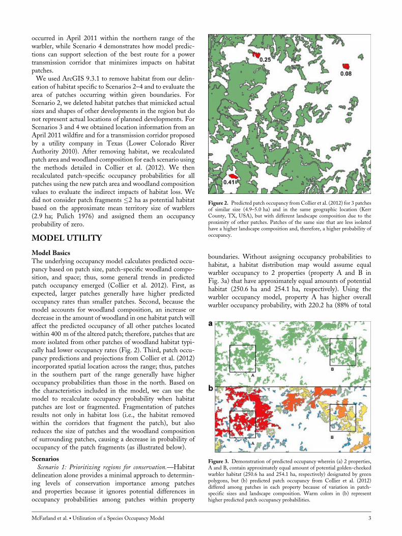
Model BasicsThe underlying occupancy model calculates predicted occu-pancy based on patch size, patch-specific woodland compo-sition, and space; thus, some general trends in predictedpatch occupancy emerged (Collier et al. 2012). First, asexpected, larger patches generally have higher predictedoccupancy rates than smaller patches. Second, because themodel accounts for woodland composition, an increase ordecrease in the amount of woodland in one habitat patch willaffect the predicted occupancy of all other patches locatedwithin 400 m of the altered patch; therefore, patches that aremore isolated from other patches of woodland habitat typi-cally had lower occupancy rates (Fig. 2). Third, patch occu-pancy predictions and projections from Collier et al. (2012)incorporated spatial location across the range; thus, patchesin the southern part of the range generally have higheroccupancy probabilities than those in the north. Based onthe characteristics included in the model, we can use themodel to recalculate occupancy probability when habitatpatches are lost or fragmented. Fragmentation of patchesresults not only in habitat loss (i.e., the habitat removedwithin the corridors that fragment the patch), but alsoreduces the size of patches and the woodland compositionof surrounding patches, causing a decrease in probability ofoccupancy of the patch fragments (as illustrated below).

ScenariosScenario 1: Prioritizing regions for conservation.—Habitat

delineation alone provides a minimal approach to determin-ing levels of conservation importance among patchesand properties because it ignores potential differences inoccupancy probabilities among patches within property

boundaries. Without assigning occupancy probabilities tohabitat, a habitat distribution map would assume equalwarbler occupancy to 2 properties (property A and B inFig. 3a) that have approximately equal amounts of potentialhabitat (250.6 ha and 254.1 ha, respectively). Using thewarbler occupancy model, property A has higher overallwarbler occupancy probability, with 220.2 ha (88% of total

Figure 2. Predicted patch occupancy from Collier et al. (2012) for 3 patchesof similar size (4.9–5.0 ha) and in the same geographic location (KerrCounty, TX, USA), but with different landscape composition due to theproximity of other patches. Patches of the same size that are less isolatedhave a higher landscape composition and, therefore, a higher probability ofoccupancy.

Figure 3. Demonstration of predicted occupancy wherein (a) 2 properties,A and B, contain approximately equal amount of potential golden-cheekedwarbler habitat (250.6 ha and 254.1 ha, respectively) designated by greenpolygons, but (b) predicted patch occupancy from Collier et al. (2012)differed among patches in each property because of variation in patch-specific sizes and landscape composition. Warm colors in (b) representhigher predicted patch occupancy probabilities.

McFarland et al. � Utilization of a Species Occupancy Model 3

area) above 93% occupancy probability, than does property B(Fig. 3b). Property B only has 75.7 ha (30% of total area)above 70% probability of occupancy, and 176.8 ha above 50%probability of occupancy.Scenario 2: Urban expansion.—Urban expansion is one of

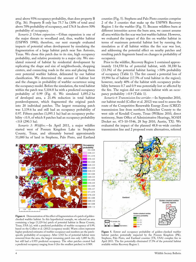
the major threats to woodland and, thus, warbler habitat(USFWS 1990); therefore, our next example evaluatedimpacts of potential urban development by simulating thefragmentation of a large habitat patch near San Antonio,Texas. We chose this patch due to its size, high occupancyprobability, and relative proximity to a major city. We sim-ulated removal of habitat by residential development byreplicating the shape and size of neighborhoods, shoppingcenters, and connecting roads in the area and placing themover potential warbler habitat, delineated by our habitatclassification. We determined the amount of habitat lostand the changes in probability of warbler occurrence usingthe occupancy model. Before the simulation, the total habitatwithin the patch was 5,104.8 ha with a predicted occupancyprobability of 0.99 (Fig. 4). We simulated 1,093.2 haof developed area, a 21.4% reduction in total habitatpostdevelopment, which fragmented the original patchinto 20 individual patches. The largest remaining patchwas 1,139.6 ha and still had an occupancy probability of0.97. Fifteen patches (1,095.1 ha) had an occupancy proba-bility <0.9, of which 8 patches had an occupancy probability<0.8 (290.3 ha).Scenario 3: Wildfire.—In April 2011, a major wildfire

started west of Possum Kingdom Lake in StephensCounty, Texas, and ultimately burned approximately51,000 ha of land in Stephens, Palo Pinto, and Eastland

counties (Fig. 5). Stephens and Palo Pinto counties comprise2 of the 3 counties that make up the USFWS RecoveryRegion 1 for the warbler (Fig. 5). Because wildfires burn atdifferent intensities across the burn area, we cannot assumeall area within the fire scar was lost warbler habitat. However,we evaluated the impact of this fire on warbler habitat interms of maximum potential habitat lost by running thesimulation as if all habitat within the fire scar was lost,and addressing the potential effect on nearby patches andresulting patch fragments based on changes in probability ofoccupancy.Prior to the wildfire, Recovery Region 1 contained approx-

imately 114,550 ha of potential habitat, with 38,180 ha(33.3%) of the potential habitat having >50% probabilityof occupancy (Table 1). The fire caused a potential loss of19,994 ha of habitat (17.5% of total habitat in the region);however, nearly 40% of the habitat with occupancy proba-bility between 0.7 and 0.9 was potentially lost or affected bythe fire. The region did not contain habitat with an occu-pancy probability >0.9 (Table 1).Scenario 4: Transmission line corridor.—In September 2010,

our habitat model (Collier et al. 2012) was used to assess theroute of the Competitive Renewable Energy Zone (CREZ)transmission line from northern Schleicher County to thewest side of Kendall County, Texas (Wilkins 2010, directtestimony, State Office of Administrative Hearings, SOAHDocket no. 473-10-5546, 28 Sep 2010, Austin, TX). Weevaluated the impact of the planned 48.8-m-wide corridortransmission line and 2 proposed route alternatives, referred

Figure 4. Demonstration of the effect of fragmentation of a patch of golden-cheeked warbler habitat. In this hypothetical example, we selected an areacontaining a large (5,129-ha) patch of potential habitat in Bexar County,Texas, USA (a), with a predicted probability of warbler occupancy of 0.99,based on the Collier et al. (2012) occupancy model. Warm colors representhigher predicted estimates of warbler occupancy and numbers are the patch-specific probability of occupancy. After 3,923 ha of potential habitat wereremoved from the area, the largest remaining patch was only 1,085 ha (b),but still had a 0.955 predicted occupancy. The other patches created hada predicted occupancy ranging from 0 (for the smallest patches) to 0.909.

Figure 5. Extent and occupancy probability of golden-cheeked warblerhabitat patches potentially impacted by the Possum Kingdom (PK),Stephens, Palo Pinto, and Eastland counties (TX, USA) complex fire inApril 2011. The fire potentially eliminated 17.5% of the potential habitatavailable within Recovery Region 1.

4 Wildlife Society Bulletin

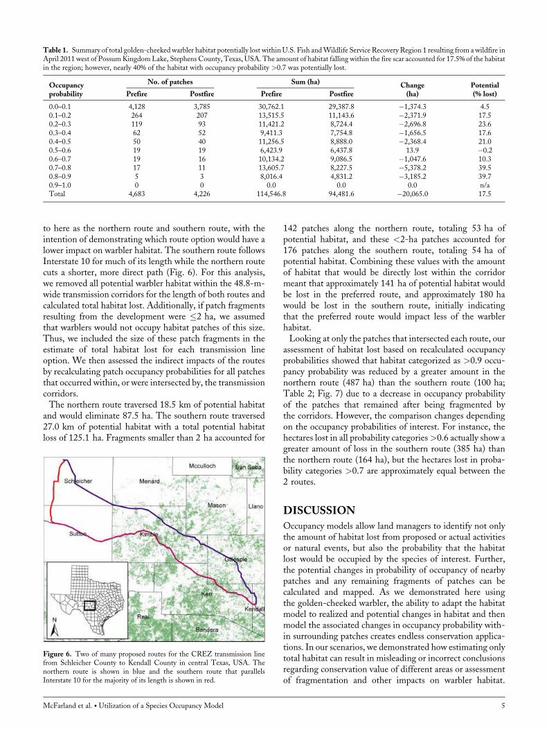
to here as the northern route and southern route, with theintention of demonstrating which route option would have alower impact on warbler habitat. The southern route followsInterstate 10 for much of its length while the northern routecuts a shorter, more direct path (Fig. 6). For this analysis,we removed all potential warbler habitat within the 48.8-m-wide transmission corridors for the length of both routes andcalculated total habitat lost. Additionally, if patch fragmentsresulting from the development were �2 ha, we assumedthat warblers would not occupy habitat patches of this size.Thus, we included the size of these patch fragments in theestimate of total habitat lost for each transmission lineoption. We then assessed the indirect impacts of the routesby recalculating patch occupancy probabilities for all patchesthat occurred within, or were intersected by, the transmissioncorridors.The northern route traversed 18.5 km of potential habitat

and would eliminate 87.5 ha. The southern route traversed27.0 km of potential habitat with a total potential habitatloss of 125.1 ha. Fragments smaller than 2 ha accounted for

142 patches along the northern route, totaling 53 ha ofpotential habitat, and these <2-ha patches accounted for176 patches along the southern route, totaling 54 ha ofpotential habitat. Combining these values with the amountof habitat that would be directly lost within the corridormeant that approximately 141 ha of potential habitat wouldbe lost in the preferred route, and approximately 180 hawould be lost in the southern route, initially indicatingthat the preferred route would impact less of the warblerhabitat.Looking at only the patches that intersected each route, our

assessment of habitat lost based on recalculated occupancyprobabilities showed that habitat categorized as >0.9 occu-pancy probability was reduced by a greater amount in thenorthern route (487 ha) than the southern route (100 ha;Table 2; Fig. 7) due to a decrease in occupancy probabilityof the patches that remained after being fragmented bythe corridors. However, the comparison changes dependingon the occupancy probabilities of interest. For instance, thehectares lost in all probability categories>0.6 actually show agreater amount of loss in the southern route (385 ha) thanthe northern route (164 ha), but the hectares lost in proba-bility categories >0.7 are approximately equal between the2 routes.

DISCUSSION

Occupancy models allow land managers to identify not onlythe amount of habitat lost from proposed or actual activitiesor natural events, but also the probability that the habitatlost would be occupied by the species of interest. Further,the potential changes in probability of occupancy of nearbypatches and any remaining fragments of patches can becalculated and mapped. As we demonstrated here usingthe golden-cheeked warbler, the ability to adapt the habitatmodel to realized and potential changes in habitat and thenmodel the associated changes in occupancy probability with-in surrounding patches creates endless conservation applica-tions. In our scenarios, we demonstrated how estimating onlytotal habitat can result in misleading or incorrect conclusionsregarding conservation value of different areas or assessmentof fragmentation and other impacts on warbler habitat.

Table 1. Summary of total golden-cheeked warbler habitat potentially lost within U.S. Fish andWildlife Service Recovery Region 1 resulting from a wildfire inApril 2011 west of PossumKingdomLake, Stephens County, Texas, USA. The amount of habitat falling within the fire scar accounted for 17.5% of the habitatin the region; however, nearly 40% of the habitat with occupancy probability >0.7 was potentially lost.

Occupancyprobability

No. of patches Sum (ha) Change(ha)

Potential(% lost)Prefire Postfire Prefire Postfire

0.0–0.1 4,128 3,785 30,762.1 29,387.8 �1,374.3 4.50.1–0.2 264 207 13,515.5 11,143.6 �2,371.9 17.50.2–0.3 119 93 11,421.2 8,724.4 �2,696.8 23.60.3–0.4 62 52 9,411.3 7,754.8 �1,656.5 17.60.4–0.5 50 40 11,256.5 8,888.0 �2,368.4 21.00.5–0.6 19 19 6,423.9 6,437.8 13.9 �0.20.6–0.7 19 16 10,134.2 9,086.5 �1,047.6 10.30.7–0.8 17 11 13,605.7 8,227.5 �5,378.2 39.50.8–0.9 5 3 8,016.4 4,831.2 �3,185.2 39.70.9–1.0 0 0 0.0 0.0 0.0 n/aTotal 4,683 4,226 114,546.8 94,481.6 �20,065.0 17.5

Figure 6. Two of many proposed routes for the CREZ transmission linefrom Schleicher County to Kendall County in central Texas, USA. Thenorthern route is shown in blue and the southern route that parallelsInterstate 10 for the majority of its length is shown in red.

McFarland et al. � Utilization of a Species Occupancy Model 5

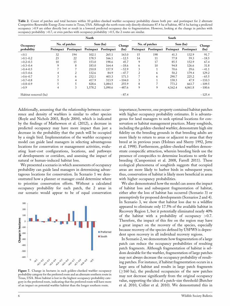
Additionally, assuming that the relationship between occur-rence and density of warblers is similar to other species(Royle and Nichols 2003, Royle 2004), which is indicatedby the findings of Mathewson et al. (2012), a decrease inpredicted occupancy may have more impact than just adecrease in the probability that the patch will be occupiedby a single bird. Implementation of the warbler occupancymodel can guide land managers in selecting advantageouslocations for conservation or management activities, evalu-ating least-cost configurations, locations, and pathwaysof developments or corridors, and assessing the impact ofnatural or human-induced habitat loss.We presented a scenario in which assessments of occupancy

probability can guide land managers in determining advan-tageous locations for conservation. In Scenario 1 we dem-onstrated how a planner or manager could determine whereto prioritize conservation efforts. Without a calculatedoccupancy probability for each patch, the 2 areas inour scenario would appear to be of equal conservation

importance; however, one property contained habitat patcheswith higher occupancy probability estimates. It is advanta-geous for land managers to seek optimal locations for con-servation or habitat management practices. Many songbirds,including the golden-cheeked warbler, demonstrate high sitefidelity on the breeding grounds in that breeding adults aremore likely to return to areas or adjacent to areas that theybreed at in previous years (Holmes and Sherry 1992, Jetteet al. 1998). Furthermore, golden-cheeked warblers demon-strate conspecific attraction, wherein breeding birds use thepresence of conspecifics to determine locations to settle forbreeding (Campomizzi et al. 2008, Farrell 2011). Theseecological phenomena of songbirds suggests that occupiedareas are more likely to harbor birds in subsequent years;thus, conservation of habitat is likely more beneficial in areaswith higher occupancy probabilities.We also demonstrated how the model can assess the impact

of habitat loss and subsequent fragmentation of habitat,either after the loss of habitat has occurred (Scenario 3) orpreemptively for proposed developments (Scenarios 2 and 4).In Scenario 3, we show that habitat loss due to a wildfireappeared to eliminate only 17.5% of the available habitat inRecovery Region 1, but it potentially eliminated nearly 40%of the habitat with a probability of occupancy >0.7.Therefore, the impact of this fire on the region may havea great impact on the recovery of the species, especiallybecause recovery of the species defined by USFWS is depen-dent upon recovery in all individual recovery regions.In Scenario 2, we demonstrate how fragmentation of a large

patch can reduce the occupancy probabilities of resultingpatch fragments. Although fragmentation of habitat is sel-dom desirable for the warbler, fragmentation of large patchesmay not always decrease the occupancy probability of result-ing patches. For instance, if habitat fragmentation occurs in alarge area of habitat and results in large patch fragments(�160 ha), the predicted occupancies of the new patchesmay not decrease significantly from the original occupancyvalue, supporting the idea of a patch-size threshold (Butcheret al. 2010, Collier et al. 2010). We demonstrated this in

Table 2. Count of patches and total hectares within 10 golden-cheeked warbler occupancy probability classes both pre- and postimpact for 2 alternateCompetitive Renewable Energy Zone routes in Texas, USA. Although the north route only directly eliminates 87.4 ha of habitat, 487.6 ha having a predictedoccupancy >0.9 are either directly lost or result in a lowered predicted occupancy due to fragmentation. However, looking at the change in patches withoccupancy probability >0.7, or even patches with occupancy probability >0.5, the 2 routes are similar.

Occupancyprobability

North South

No. of patches Sum (ha) Change(ha)

No. of patches Sum (ha) Change(ha)Preimpact Postimpact Preimpact Postimpact Preimpact Postimpact Preimpact Postimpact

<0.1 32 194 102.1 265.1 163.0 15 198 41.3 132.9 91.7>0.1–0.2 23 22 178.5 166.1 �12.5 14 11 77.8 59.3 �18.5>0.2–0.3 10 15 153.0 198.6 45.7 9 17 85.5 152.9 67.4>0.3–0.4 9 8 183.0 164.4 �18.6 6 10 94.8 126.6 31.8>0.4–0.5 7 7 210.8 157.9 �52.9 3 1 70.6 29.6 �41.1>0.5–0.6 4 2 132.6 84.9 �47.7 2 6 50.2 179.4 129.2>0.6–0.7 3 6 232.1 403.3 171.3 7 6 290.7 225.2 �65.5>0.7–0.8 5 4 417.9 313.9 �104.0 3 1 158.3 47.9 �110.3>0.8–0.9 5 5 828.6 1,084.5 255.9 8 7 773.2 663.7 �109.5>0.9 4 3 1,578.2 1,090.6 �487.6 9 9 4,162.4 4,061.8 �100.6

Habitat removed (ha) �87.4 �125.4

Figure 7. Change in hectares in each golden-cheeked warbler occupancyprobability category for the preferred route and an alternate southern route inTexas, USA. More habitat is lost in the highest occupancy-probability cate-gory in the preferred route, indicating that the preferred route will have moreof an impact on potential warbler habitat than the longer southern route.

6 Wildlife Society Bulletin

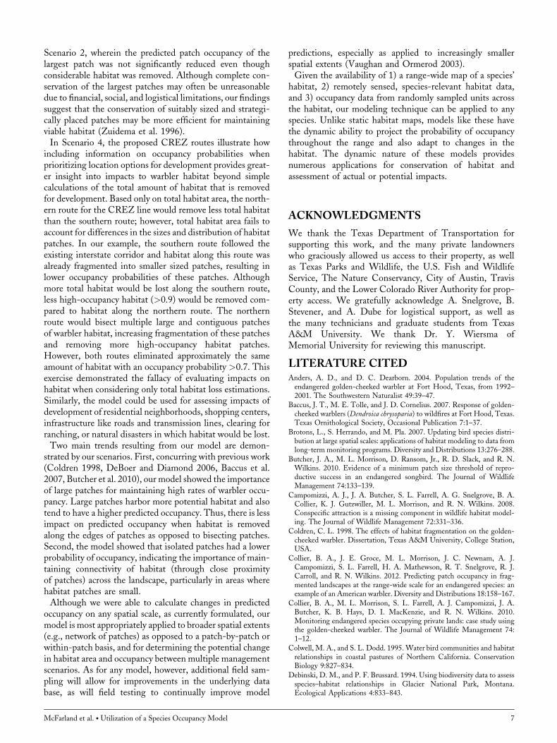
Scenario 2, wherein the predicted patch occupancy of thelargest patch was not significantly reduced even thoughconsiderable habitat was removed. Although complete con-servation of the largest patches may often be unreasonabledue to financial, social, and logistical limitations, our findingssuggest that the conservation of suitably sized and strategi-cally placed patches may be more efficient for maintainingviable habitat (Zuidema et al. 1996).In Scenario 4, the proposed CREZ routes illustrate how

including information on occupancy probabilities whenprioritizing location options for development provides great-er insight into impacts to warbler habitat beyond simplecalculations of the total amount of habitat that is removedfor development. Based only on total habitat area, the north-ern route for the CREZ line would remove less total habitatthan the southern route; however, total habitat area fails toaccount for differences in the sizes and distribution of habitatpatches. In our example, the southern route followed theexisting interstate corridor and habitat along this route wasalready fragmented into smaller sized patches, resulting inlower occupancy probabilities of these patches. Althoughmore total habitat would be lost along the southern route,less high-occupancy habitat (>0.9) would be removed com-pared to habitat along the northern route. The northernroute would bisect multiple large and contiguous patchesof warbler habitat, increasing fragmentation of these patchesand removing more high-occupancy habitat patches.However, both routes eliminated approximately the sameamount of habitat with an occupancy probability >0.7. Thisexercise demonstrated the fallacy of evaluating impacts onhabitat when considering only total habitat loss estimations.Similarly, the model could be used for assessing impacts ofdevelopment of residential neighborhoods, shopping centers,infrastructure like roads and transmission lines, clearing forranching, or natural disasters in which habitat would be lost.Two main trends resulting from our model are demon-

strated by our scenarios. First, concurring with previous work(Coldren 1998, DeBoer and Diamond 2006, Baccus et al.2007, Butcher et al. 2010), our model showed the importanceof large patches for maintaining high rates of warbler occu-pancy. Large patches harbor more potential habitat and alsotend to have a higher predicted occupancy. Thus, there is lessimpact on predicted occupancy when habitat is removedalong the edges of patches as opposed to bisecting patches.Second, the model showed that isolated patches had a lowerprobability of occupancy, indicating the importance of main-taining connectivity of habitat (through close proximityof patches) across the landscape, particularly in areas wherehabitat patches are small.Although we were able to calculate changes in predicted

occupancy on any spatial scale, as currently formulated, ourmodel is most appropriately applied to broader spatial extents(e.g., network of patches) as opposed to a patch-by-patch orwithin-patch basis, and for determining the potential changein habitat area and occupancy between multiple managementscenarios. As for any model, however, additional field sam-pling will allow for improvements in the underlying database, as will field testing to continually improve model

predictions, especially as applied to increasingly smallerspatial extents (Vaughan and Ormerod 2003).Given the availability of 1) a range-wide map of a species’

habitat, 2) remotely sensed, species-relevant habitat data,and 3) occupancy data from randomly sampled units acrossthe habitat, our modeling technique can be applied to anyspecies. Unlike static habitat maps, models like these havethe dynamic ability to project the probability of occupancythroughout the range and also adapt to changes in thehabitat. The dynamic nature of these models providesnumerous applications for conservation of habitat andassessment of actual or potential impacts.

ACKNOWLEDGMENTS

We thank the Texas Department of Transportation forsupporting this work, and the many private landownerswho graciously allowed us access to their property, as wellas Texas Parks and Wildlife, the U.S. Fish and WildlifeService, The Nature Conservancy, City of Austin, TravisCounty, and the Lower Colorado River Authority for prop-erty access. We gratefully acknowledge A. Snelgrove, B.Stevener, and A. Dube for logistical support, as well asthe many technicians and graduate students from TexasA&M University. We thank Dr. Y. Wiersma ofMemorial University for reviewing this manuscript.

LITERATURE CITEDAnders, A. D., and D. C. Dearborn. 2004. Population trends of theendangered golden-cheeked warbler at Fort Hood, Texas, from 1992–2001. The Southwestern Naturalist 49:39–47.

Baccus, J. T., M. E. Tolle, and J. D. Cornelius. 2007. Response of golden-cheeked warblers (Dendroica chrysoparia) to wildfires at Fort Hood, Texas.Texas Ornithological Society, Occasional Publication 7:1–37.

Brotons, L., S. Herrando, and M. Pla. 2007. Updating bird species distri-bution at large spatial scales: applications of habitat modeling to data fromlong-term monitoring programs. Diversity and Distributions 13:276–288.

Butcher, J. A., M. L. Morrison, D. Ransom, Jr., R. D. Slack, and R. N.Wilkins. 2010. Evidence of a minimum patch size threshold of repro-ductive success in an endangered songbird. The Journal of WildlifeManagement 74:133–139.

Campomizzi, A. J., J. A. Butcher, S. L. Farrell, A. G. Snelgrove, B. A.Collier, K. J. Gutzwiller, M. L. Morrison, and R. N. Wilkins. 2008.Conspecific attraction is a missing component in wildlife habitat model-ing. The Journal of Wildlife Management 72:331–336.

Coldren, C. L. 1998. The effects of habitat fragmentation on the golden-cheeked warbler. Dissertation, Texas A&M University, College Station,USA.

Collier, B. A., J. E. Groce, M. L. Morrison, J. C. Newnam, A. J.Campomizzi, S. L. Farrell, H. A. Mathewson, R. T. Snelgrove, R. J.Carroll, and R. N. Wilkins. 2012. Predicting patch occupancy in frag-mented landscapes at the range-wide scale for an endangered species: anexample of an American warbler. Diversity and Distributions 18:158–167.

Collier, B. A., M. L. Morrison, S. L. Farrell, A. J. Campomizzi, J. A.Butcher, K. B. Hays, D. I. MacKenzie, and R. N. Wilkins. 2010.Monitoring endangered species occupying private lands: case study usingthe golden-cheeked warbler. The Journal of Wildlife Management 74:1–12.

Colwell, M. A., and S. L. Dodd. 1995. Water bird communities and habitatrelationships in coastal pastures of Northern California. ConservationBiology 9:827–834.

Debinski, D. M., and P. F. Brussard. 1994. Using biodiversity data to assessspecies–habitat relationships in Glacier National Park, Montana.Ecological Applications 4:833–843.

McFarland et al. � Utilization of a Species Occupancy Model 7

DeBoer, T. S., and D. D. Diamond. 2006. Predicting presence–absenceof the endangered golden-cheeked warbler (Dendroica chrysoparia). TheSouthwestern Naturalist 51:181–190.

Diamond, D. D. 2007. Range-wide modeling of golden-cheeked warblerhabitat. Technical report, Texas Parks and Wildlife Department, Austin,Texas, USA.

Farrell, S. L. 2011. Use of social information for habitat selectionin songbirds. Dissertation, Texas A&M University, College Station,USA.

Gobeil, J.-F., and M.-A. Villard. 2002. Permeability of three boreal forestlandscape types to bird movements as determined from experimentaltranslocations. Oikos 98:447–458.

Goodwin, B. J., and L. Fahrig. 2002.How does landscape structure influencelandscape connectivity? Oikos 99:552–570.

Haynes, K. J., and J. T. Cronin. 2006. Inter-patch movement and edgeeffects: the role of behavioral responses to the landscape matrix. Oikos113:43–54.

Holmes, R. T., and T.W. Sherry. 1992. Site fidelity of migratory warblers intemperate breeding and Neotropical wintering areas: implications forpopulation dynamics, habitat selection, and conservation. Pages 563–575 in J. M. Hagan and D. W. Johnston, editors. Ecology and conserva-tion of Neotropical migrant land birds. Smithsonian Institution Press,Washington, D.C., USA.

Homer, C., J. Dewitz, J. Fry, M. Coan, N. Hossain, C. Larson, N. Herold,A. McKerrow, J. N. VanDriel, and J. Wickham. 2007. Completion of the2001 national land cover database for the conterminous United States.Photogrammetric Engineering and Remote Sensing 73:337–341.

Jette, L. A., T. J. Hayden, and J. D. Cornelius. 1998. Demographics of thegolden-cheeked warbler (Dendroica chrysoparia) on FortHood, Texas. U.S.ArmyCorps of Engineers, U.S. ArmyConstruction Engineering ResearchLaboratory Technical Report 98/52, Fort Hood, Texas, USA.

Kantrud, H. A., and R. E. Stewart. 1984. Ecological distribution and crudedensity of breeding birds on prairie wetlands. The Journal of WildlifeManagement 48:426–437.

Lower Colorado River Authority. 2010. Lower Colorado River Authorityand Competitive Renewable Energy Zones. <www.lcra.org/CREZ>Accessed 1 Sep 2010.

Loomis-Austin, Inc. 2008. Mapping potential golden-cheeked warblerbreeding habitat using remotely sensed forest canopy cover data.County of Hays, San Marcos, Texas, USA.

Magness, D. R., R. N. Wilkins, and S. J. Hejl. 2006. Quantitative relation-ships among golden-cheeked warbler occurrence and landscape size,composition, and structure. Wildlife Society Bulletin 34:473–479.

Mathewson, H. A., J. E. Groce, T. M. McFarland, M. L. Morrison, J. C.Newnam, R. T. Snelgrove, B. A. Collier, and R. N. Wilkins. 2012.Estimating breeding season abundance of golden-cheeked warblers inTexas. Journal of Wildlife Management 76:in press.

Peak, R. G. 2007. Forest edges negatively affect golden-cheeked warblernest survival. The Condor 109:628–637.

Pulich, W. M. 1976. The golden-cheeked warbler: a bioecological study.Texas Parks and Wildlife Department, Austin, USA.

Rappole, J. H., D. I. King, and J. Diez. 2003. Winter- vs. breeding-habitatlimitation for an endangered avian migrant. Ecological Applications13:735–742.

Reidy, J. L., M. M. Stake, and F. R. Thompson, III. 2008. Golden-cheekedwarbler nest mortality and predators in urban and rural landscapes. TheCondor 110:458–466.

Richard, Y., and D. Armstrong. 2010. The importance of integratinglandscape ecology in habitat models: isolation-driven occurrence of northisland robins in a fragmented landscape. Landscape Ecology 25:1363–1374.

Rowell, G. A., D. P. Keddy-Hector, D. D. Diamond, J. Lloyd, B.McKinney, R. C. Maggio, and T. L. Cook. 1995. Remote sensing andGIS of golden-cheeked warbler breeding habitat and vegetation types onthe Edwards Plateau. Texas Parks and Wildlife Department, Austin,USA.

Royle, J. A. 2004. Modeling abundance index data from anuran callingsurveys. Conservation Biology 18:1378–1385.

Royle, J. A., and J. D. Nichols. 2003. Estimating abundance from repeatedpresence–absence data or point counts. Ecology 84:777–790.

Sagarin, R. D., S. D. Gaines, and B. Gaylord. 2006. Moving beyondassumptions to understand abundance distributions across the ranges ofspecies. Trends in Ecology & Evolution 21:524–530.

United States Fish and Wildlife Service [USFWS]. 1990. Endangered andthreatened wildlife and plants; final rule to list the golden-cheeked warbleras endangered. Federal Register 55:53153–53160.

United States Fish and Wildlife Service [USFWS]. 1992. Golden-cheekedwarbler (Dendroica chrysoparia) recovery plan. U.S. Fish and WildlifeService, Austin, Texas, USA.

Vaughan, I. P., and S. J. Ormerod. 2003. Improving the quality of distribu-tion models for conservation by addressing shortcomings in the fieldcollection of training data. Conservation Biology 17:1601–1611.

Wahl, R., D. D. Diamond, and D. Shaw. 1990. The golden-cheekedwarbler: a status review. Texas Parks and Wildlife Department, Austin,USA.

Wiens, J. A., and J. T. Rotenberry. 1985. Response of breeding passerinebirds to rangeland alteration in a North American shrub steppe locality.Journal of Applied Ecology 22:655–668.

Zuidema, P. A., J. A. Sayer, and W. Dijkman. 1996. Forest fragmentationand biodiversity: the case for intermediate-sized conservation areas.Environmental Conservation 23:290–297.

Associate Editor: White.

8 Wildlife Society Bulletin

BIODIVERSITYRESEARCH

Predicting patch occupancy in fragmentedlandscapes at the rangewide scale for anendangered species: an example of anAmerican warbler

Bret A. Collier1*, Julie E. Groce2, Michael L. Morrison3, John C. Newnam4,

Andrew J. Campomizzi3, Shannon L. Farrell3, Heather A. Mathewson1,

Robert T. Snelgrove1, Raymond J. Carroll5 and Robert N. Wilkins1

INTRODUCTION

Species inhabiting human-dominated environments often exist

in locations where habitat loss and fragmentation have reduced

patch contiguity, patch size, and increased edge and isolation

effects (Marzluff, 2001; Bolger, 2002). Such changes in

structural features at the local scale also influence dynamics

in surrounding areas (Forman, 1995; Saab, 1999). Moreover,

1Institute of Renewable Natural Resources,

Texas A and M University, College Station,

TX 77843, USA, 2Institute of Renewable

Natural Resources, Texas A and M University,

San Antonio, TX 77843, USA, 3Department of

Wildlife and Fisheries Sciences, Texas A and

M University, College Station, TX 77843,

USA, 4Texas Department of Transportation,

PO Box 15426, Austin, TX 78761, USA,5Department of Statistics, Texas A and M

University, College Station, TX 77843, USA

*Correspondence: Bret A. Collier, Institute of

Renewable Natural Resources, Texas A&M

University, College Station, TX 77843, USA.

E-mail: bret@tamu.edu

ABSTRACT

Aim Our objective was to identify the distribution of the endangered golden-

cheeked warbler (Setophaga chrysoparia) in fragmented oak–juniper woodlands by

applying a geoadditive semiparametric occupancy model to better assist decision-

makers in identifying suitable habitat across the species breeding range on which

conservation or mitigation activities can be focused and thus prioritize

management and conservation planning.

Location Texas, USA.

Methods We used repeated double-observer detection/non-detection surveys of

randomly selected (n = 287) patches of potential habitat to evaluate warbler

patch-scale presence across the species breeding range. We used a geoadditive

semiparametric occupancy model with remotely sensed habitat metrics (patch size

and landscape composition) to predict patch-scale occupancy of golden-cheeked

warblers in the fragmented oak–juniper woodlands of central Texas, USA.

Results Our spatially explicit model indicated that golden-cheeked warbler patch

occupancy declined from south to north within the breeding range concomitant

with reductions in the availability of large habitat patches. We found that 59% of

woodland patches, primarily in the northern and central portions of the warbler’s

range, were predicted to have occupancy probabilities £0.10 with only 3% of

patches predicted to have occupancy probabilities >0.90. Our model exhibited

high prediction accuracy (area under curve = 0.91) when validated using

independently collected warbler occurrence data.

Main conclusions We have identified a distinct spatial occurrence gradient for

golden-cheeked warblers as well as a relationship between two measurable

landscape characteristics. Because habitat-occupancy relationships were key

drivers of our model, our results can be used to identify potential areas where

conservation actions supporting habitat mitigation can occur and identify areas

where conservation of future potential habitat is possible. Additionally, our results

can be used to focus resources on maintenance and creation of patches that are

more likely to harbour viable local warbler populations.

Keywords

Bayesian inference, golden-cheeked warbler, habitat conservation, occupancy,

semiparametric regression, Setophaga chrysoparia.

Diversity and Distributions, (Diversity Distrib.) (2012) 18, 158–167

DOI:10.1111/j.1472-4642.2011.00831.x158 http://wileyonlinelibrary.com/journal/ddi ª 2011 Blackwell Publishing Ltd

A J

ourn

al o

f Co

nser

vati

on B

ioge

ogra

phy

Div

ersi

ty a

nd D

istr

ibut

ions

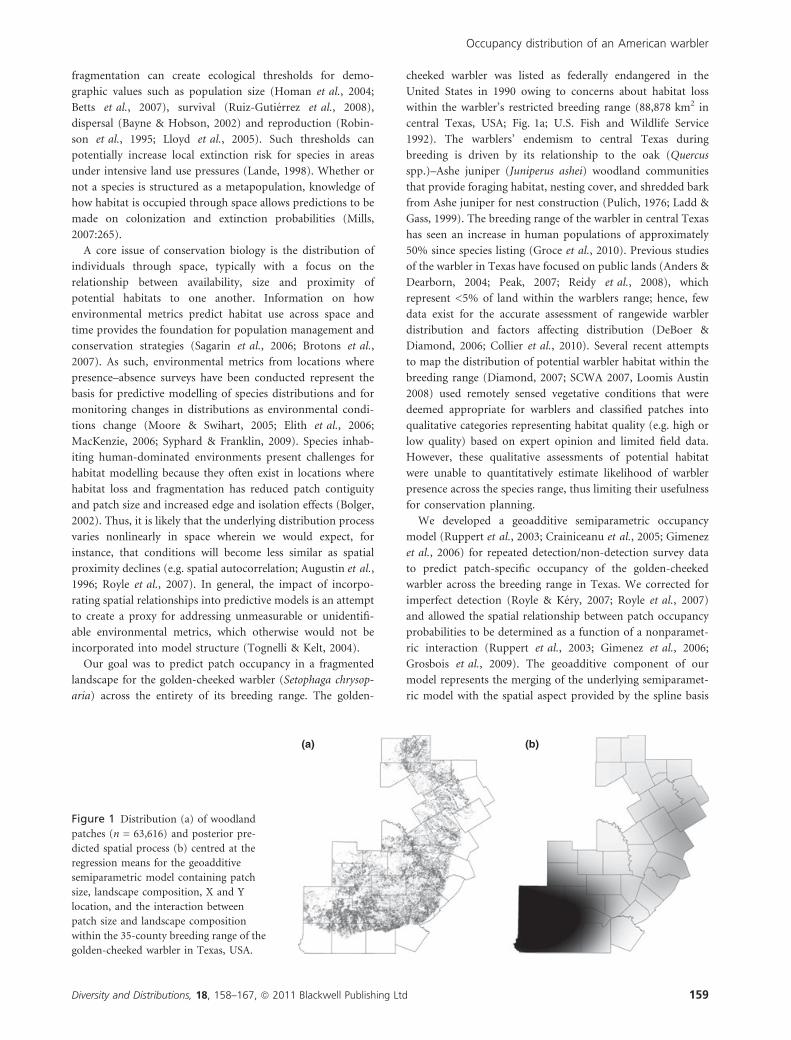
fragmentation can create ecological thresholds for demo-

graphic values such as population size (Homan et al., 2004;

Betts et al., 2007), survival (Ruiz-Gutierrez et al., 2008),

dispersal (Bayne & Hobson, 2002) and reproduction (Robin-

son et al., 1995; Lloyd et al., 2005). Such thresholds can

potentially increase local extinction risk for species in areas

under intensive land use pressures (Lande, 1998). Whether or

not a species is structured as a metapopulation, knowledge of

how habitat is occupied through space allows predictions to be

made on colonization and extinction probabilities (Mills,

2007:265).

A core issue of conservation biology is the distribution of

individuals through space, typically with a focus on the

relationship between availability, size and proximity of

potential habitats to one another. Information on how

environmental metrics predict habitat use across space and

time provides the foundation for population management and

conservation strategies (Sagarin et al., 2006; Brotons et al.,

2007). As such, environmental metrics from locations where

presence–absence surveys have been conducted represent the

basis for predictive modelling of species distributions and for

monitoring changes in distributions as environmental condi-

tions change (Moore & Swihart, 2005; Elith et al., 2006;

MacKenzie, 2006; Syphard & Franklin, 2009). Species inhab-

iting human-dominated environments present challenges for

habitat modelling because they often exist in locations where

habitat loss and fragmentation has reduced patch contiguity

and patch size and increased edge and isolation effects (Bolger,

2002). Thus, it is likely that the underlying distribution process

varies nonlinearly in space wherein we would expect, for

instance, that conditions will become less similar as spatial

proximity declines (e.g. spatial autocorrelation; Augustin et al.,

1996; Royle et al., 2007). In general, the impact of incorpo-

rating spatial relationships into predictive models is an attempt

to create a proxy for addressing unmeasurable or unidentifi-

able environmental metrics, which otherwise would not be

incorporated into model structure (Tognelli & Kelt, 2004).

Our goal was to predict patch occupancy in a fragmented

landscape for the golden-cheeked warbler (Setophaga chrysop-

aria) across the entirety of its breeding range. The golden-

cheeked warbler was listed as federally endangered in the

United States in 1990 owing to concerns about habitat loss

within the warbler’s restricted breeding range (88,878 km2 in

central Texas, USA; Fig. 1a; U.S. Fish and Wildlife Service

1992). The warblers’ endemism to central Texas during

breeding is driven by its relationship to the oak (Quercus

spp.)–Ashe juniper (Juniperus ashei) woodland communities

that provide foraging habitat, nesting cover, and shredded bark

from Ashe juniper for nest construction (Pulich, 1976; Ladd &

Gass, 1999). The breeding range of the warbler in central Texas

has seen an increase in human populations of approximately

50% since species listing (Groce et al., 2010). Previous studies

of the warbler in Texas have focused on public lands (Anders &

Dearborn, 2004; Peak, 2007; Reidy et al., 2008), which

represent <5% of land within the warblers range; hence, few

data exist for the accurate assessment of rangewide warbler

distribution and factors affecting distribution (DeBoer &

Diamond, 2006; Collier et al., 2010). Several recent attempts

to map the distribution of potential warbler habitat within the

breeding range (Diamond, 2007; SCWA 2007, Loomis Austin

2008) used remotely sensed vegetative conditions that were

deemed appropriate for warblers and classified patches into

qualitative categories representing habitat quality (e.g. high or

low quality) based on expert opinion and limited field data.

However, these qualitative assessments of potential habitat

were unable to quantitatively estimate likelihood of warbler

presence across the species range, thus limiting their usefulness

for conservation planning.

We developed a geoadditive semiparametric occupancy

model (Ruppert et al., 2003; Crainiceanu et al., 2005; Gimenez

et al., 2006) for repeated detection/non-detection survey data

to predict patch-specific occupancy of the golden-cheeked

warbler across the breeding range in Texas. We corrected for

imperfect detection (Royle & Kery, 2007; Royle et al., 2007)

and allowed the spatial relationship between patch occupancy

probabilities to be determined as a function of a nonparamet-

ric interaction (Ruppert et al., 2003; Gimenez et al., 2006;

Grosbois et al., 2009). The geoadditive component of our

model represents the merging of the underlying semiparamet-

ric model with the spatial aspect provided by the spline basis

(a) (b)

Figure 1 Distribution (a) of woodland

patches (n = 63,616) and posterior pre-

dicted spatial process (b) centred at the

regression means for the geoadditive

semiparametric model containing patch

size, landscape composition, X and Y

location, and the interaction between

patch size and landscape composition

within the 35-county breeding range of the

golden-cheeked warbler in Texas, USA.

Occupancy distribution of an American warbler

Diversity and Distributions, 18, 158–167, ª 2011 Blackwell Publishing Ltd 159

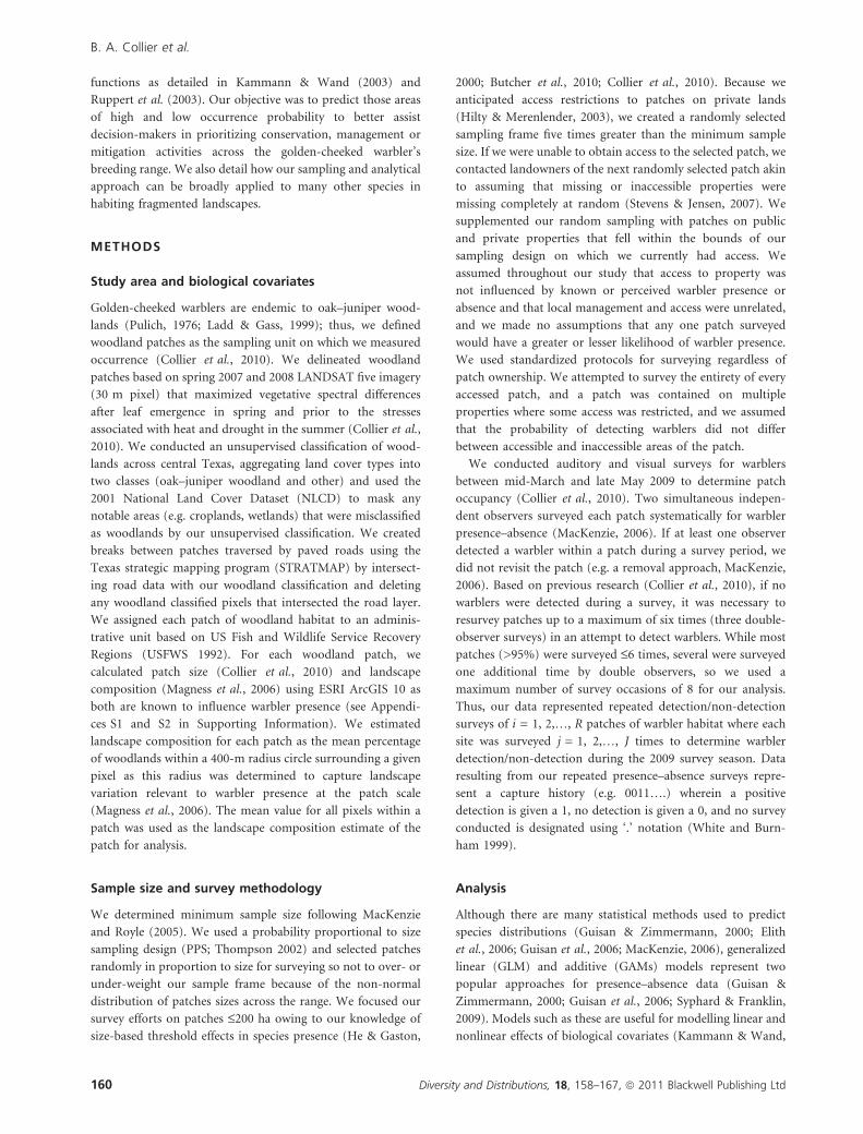
functions as detailed in Kammann & Wand (2003) and

Ruppert et al. (2003). Our objective was to predict those areas

of high and low occurrence probability to better assist

decision-makers in prioritizing conservation, management or

mitigation activities across the golden-cheeked warbler’s

breeding range. We also detail how our sampling and analytical

approach can be broadly applied to many other species in

habiting fragmented landscapes.

METHODS

Study area and biological covariates

Golden-cheeked warblers are endemic to oak–juniper wood-

lands (Pulich, 1976; Ladd & Gass, 1999); thus, we defined

woodland patches as the sampling unit on which we measured

occurrence (Collier et al., 2010). We delineated woodland

patches based on spring 2007 and 2008 LANDSAT five imagery

(30 m pixel) that maximized vegetative spectral differences

after leaf emergence in spring and prior to the stresses

associated with heat and drought in the summer (Collier et al.,

2010). We conducted an unsupervised classification of wood-

lands across central Texas, aggregating land cover types into

two classes (oak–juniper woodland and other) and used the

2001 National Land Cover Dataset (NLCD) to mask any

notable areas (e.g. croplands, wetlands) that were misclassified

as woodlands by our unsupervised classification. We created

breaks between patches traversed by paved roads using the

Texas strategic mapping program (STRATMAP) by intersect-

ing road data with our woodland classification and deleting

any woodland classified pixels that intersected the road layer.

We assigned each patch of woodland habitat to an adminis-

trative unit based on US Fish and Wildlife Service Recovery

Regions (USFWS 1992). For each woodland patch, we

calculated patch size (Collier et al., 2010) and landscape

composition (Magness et al., 2006) using ESRI ArcGIS 10 as

both are known to influence warbler presence (see Appendi-

ces S1 and S2 in Supporting Information). We estimated

landscape composition for each patch as the mean percentage

of woodlands within a 400-m radius circle surrounding a given

pixel as this radius was determined to capture landscape

variation relevant to warbler presence at the patch scale

(Magness et al., 2006). The mean value for all pixels within a

patch was used as the landscape composition estimate of the

patch for analysis.

Sample size and survey methodology

We determined minimum sample size following MacKenzie

and Royle (2005). We used a probability proportional to size

sampling design (PPS; Thompson 2002) and selected patches

randomly in proportion to size for surveying so not to over- or

under-weight our sample frame because of the non-normal

distribution of patches sizes across the range. We focused our

survey efforts on patches £200 ha owing to our knowledge of

size-based threshold effects in species presence (He & Gaston,

2000; Butcher et al., 2010; Collier et al., 2010). Because we

anticipated access restrictions to patches on private lands

(Hilty & Merenlender, 2003), we created a randomly selected

sampling frame five times greater than the minimum sample

size. If we were unable to obtain access to the selected patch, we

contacted landowners of the next randomly selected patch akin

to assuming that missing or inaccessible properties were

missing completely at random (Stevens & Jensen, 2007). We

supplemented our random sampling with patches on public

and private properties that fell within the bounds of our

sampling design on which we currently had access. We

assumed throughout our study that access to property was

not influenced by known or perceived warbler presence or

absence and that local management and access were unrelated,

and we made no assumptions that any one patch surveyed

would have a greater or lesser likelihood of warbler presence.

We used standardized protocols for surveying regardless of

patch ownership. We attempted to survey the entirety of every

accessed patch, and a patch was contained on multiple

properties where some access was restricted, and we assumed

that the probability of detecting warblers did not differ

between accessible and inaccessible areas of the patch.

We conducted auditory and visual surveys for warblers

between mid-March and late May 2009 to determine patch

occupancy (Collier et al., 2010). Two simultaneous indepen-

dent observers surveyed each patch systematically for warbler

presence–absence (MacKenzie, 2006). If at least one observer

detected a warbler within a patch during a survey period, we

did not revisit the patch (e.g. a removal approach, MacKenzie,

2006). Based on previous research (Collier et al., 2010), if no

warblers were detected during a survey, it was necessary to

resurvey patches up to a maximum of six times (three double-

observer surveys) in an attempt to detect warblers. While most

patches (>95%) were surveyed £6 times, several were surveyed

one additional time by double observers, so we used a

maximum number of survey occasions of 8 for our analysis.

Thus, our data represented repeated detection/non-detection

surveys of i = 1, 2,…, R patches of warbler habitat where each

site was surveyed j = 1, 2,…, J times to determine warbler

detection/non-detection during the 2009 survey season. Data

resulting from our repeated presence–absence surveys repre-

sent a capture history (e.g. 0011….) wherein a positive

detection is given a 1, no detection is given a 0, and no survey

conducted is designated using ‘.’ notation (White and Burn-

ham 1999).

Analysis

Although there are many statistical methods used to predict

species distributions (Guisan & Zimmermann, 2000; Elith

et al., 2006; Guisan et al., 2006; MacKenzie, 2006), generalized

linear (GLM) and additive (GAMs) models represent two

popular approaches for presence–absence data (Guisan &

Zimmermann, 2000; Guisan et al., 2006; Syphard & Franklin,

2009). Models such as these are useful for modelling linear and

nonlinear effects of biological covariates (Kammann & Wand,

B. A. Collier et al.

160 Diversity and Distributions, 18, 158–167, ª 2011 Blackwell Publishing Ltd

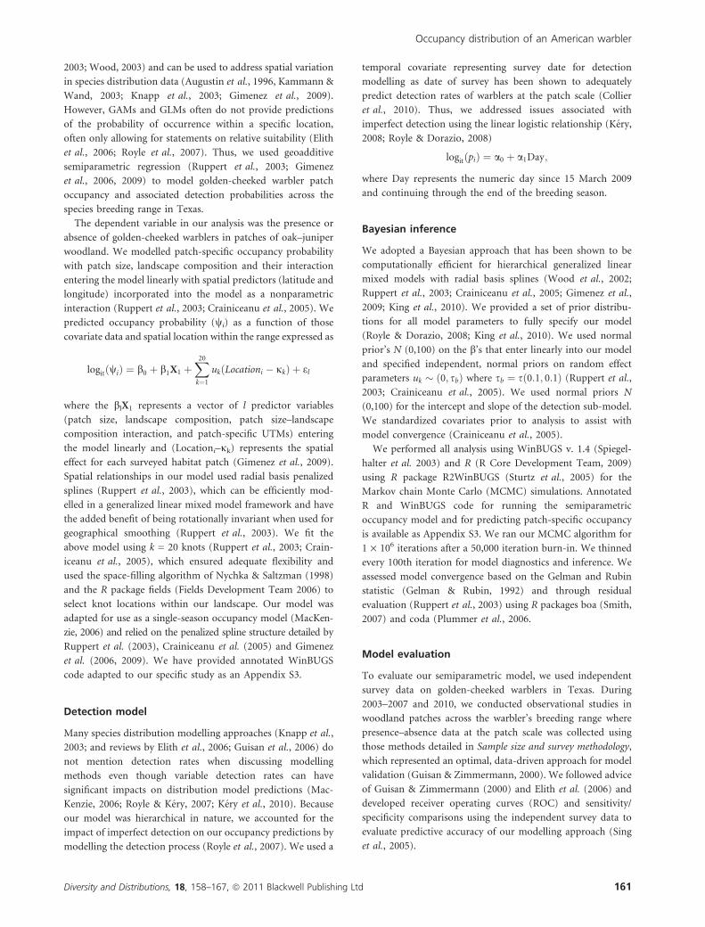
2003; Wood, 2003) and can be used to address spatial variation

in species distribution data (Augustin et al., 1996, Kammann &

Wand, 2003; Knapp et al., 2003; Gimenez et al., 2009).

However, GAMs and GLMs often do not provide predictions

of the probability of occurrence within a specific location,

often only allowing for statements on relative suitability (Elith

et al., 2006; Royle et al., 2007). Thus, we used geoadditive

semiparametric regression (Ruppert et al., 2003; Gimenez

et al., 2006, 2009) to model golden-cheeked warbler patch

occupancy and associated detection probabilities across the

species breeding range in Texas.

The dependent variable in our analysis was the presence or

absence of golden-cheeked warblers in patches of oak–juniper

woodland. We modelled patch-specific occupancy probability

with patch size, landscape composition and their interaction

entering the model linearly with spatial predictors (latitude and

longitude) incorporated into the model as a nonparametric

interaction (Ruppert et al., 2003; Crainiceanu et al., 2005). We

predicted occupancy probability (wi) as a function of those

covariate data and spatial location within the range expressed as

logitðwiÞ ¼ b0 þ b1X1 þX20

k¼1

ukðLocationi � jkÞ þ el

where the blX1 represents a vector of l predictor variables

(patch size, landscape composition, patch size–landscape

composition interaction, and patch-specific UTMs) entering

the model linearly and (Locationi–jk) represents the spatial

effect for each surveyed habitat patch (Gimenez et al., 2009).

Spatial relationships in our model used radial basis penalized

splines (Ruppert et al., 2003), which can be efficiently mod-

elled in a generalized linear mixed model framework and have

the added benefit of being rotationally invariant when used for

geographical smoothing (Ruppert et al., 2003). We fit the

above model using k = 20 knots (Ruppert et al., 2003; Crain-

iceanu et al., 2005), which ensured adequate flexibility and

used the space-filling algorithm of Nychka & Saltzman (1998)

and the R package fields (Fields Development Team 2006) to

select knot locations within our landscape. Our model was

adapted for use as a single-season occupancy model (MacKen-

zie, 2006) and relied on the penalized spline structure detailed by

Ruppert et al. (2003), Crainiceanu et al. (2005) and Gimenez

et al. (2006, 2009). We have provided annotated WinBUGS

code adapted to our specific study as an Appendix S3.

Detection model

Many species distribution modelling approaches (Knapp et al.,

2003; and reviews by Elith et al., 2006; Guisan et al., 2006) do

not mention detection rates when discussing modelling

methods even though variable detection rates can have

significant impacts on distribution model predictions (Mac-

Kenzie, 2006; Royle & Kery, 2007; Kery et al., 2010). Because

our model was hierarchical in nature, we accounted for the

impact of imperfect detection on our occupancy predictions by

modelling the detection process (Royle et al., 2007). We used a

temporal covariate representing survey date for detection

modelling as date of survey has been shown to adequately

predict detection rates of warblers at the patch scale (Collier

et al., 2010). Thus, we addressed issues associated with

imperfect detection using the linear logistic relationship (Kery,

2008; Royle & Dorazio, 2008)

logitðpiÞ ¼ a0 þ a1Day;

where Day represents the numeric day since 15 March 2009

and continuing through the end of the breeding season.

Bayesian inference

We adopted a Bayesian approach that has been shown to be

computationally efficient for hierarchical generalized linear

mixed models with radial basis splines (Wood et al., 2002;

Ruppert et al., 2003; Crainiceanu et al., 2005; Gimenez et al.,

2009; King et al., 2010). We provided a set of prior distribu-

tions for all model parameters to fully specify our model

(Royle & Dorazio, 2008; King et al., 2010). We used normal

prior’s N (0,100) on the b’s that enter linearly into our model

and specified independent, normal priors on random effect

parameters uk � ð0; sbÞ where sb ¼ sð0:1; 0:1Þ (Ruppert et al.,

2003; Crainiceanu et al., 2005). We used normal priors N

(0,100) for the intercept and slope of the detection sub-model.

We standardized covariates prior to analysis to assist with

model convergence (Crainiceanu et al., 2005).

We performed all analysis using WinBUGS v. 1.4 (Spiegel-

halter et al. 2003) and R (R Core Development Team, 2009)

using R package R2WinBUGS (Sturtz et al., 2005) for the

Markov chain Monte Carlo (MCMC) simulations. Annotated

R and WinBUGS code for running the semiparametric

occupancy model and for predicting patch-specific occupancy

is available as Appendix S3. We ran our MCMC algorithm for

1 · 106 iterations after a 50,000 iteration burn-in. We thinned

every 100th iteration for model diagnostics and inference. We

assessed model convergence based on the Gelman and Rubin

statistic (Gelman & Rubin, 1992) and through residual

evaluation (Ruppert et al., 2003) using R packages boa (Smith,

2007) and coda (Plummer et al., 2006.

Model evaluation

To evaluate our semiparametric model, we used independent

survey data on golden-cheeked warblers in Texas. During

2003–2007 and 2010, we conducted observational studies in

woodland patches across the warbler’s breeding range where

presence–absence data at the patch scale was collected using

those methods detailed in Sample size and survey methodology,

which represented an optimal, data-driven approach for model

validation (Guisan & Zimmermann, 2000). We followed advice

of Guisan & Zimmermann (2000) and Elith et al. (2006) and

developed receiver operating curves (ROC) and sensitivity/

specificity comparisons using the independent survey data to

evaluate predictive accuracy of our modelling approach (Sing

et al., 2005).

Occupancy distribution of an American warbler

Diversity and Distributions, 18, 158–167, ª 2011 Blackwell Publishing Ltd 161

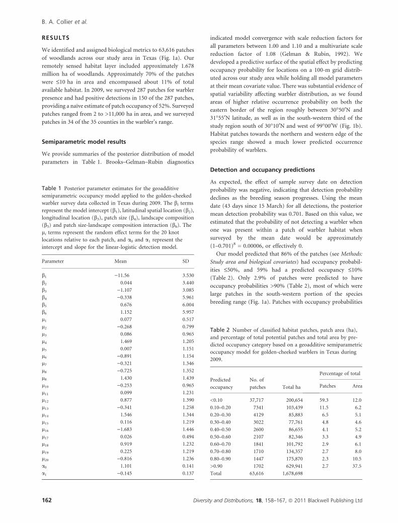
RESULTS

We identified and assigned biological metrics to 63,616 patches

of woodlands across our study area in Texas (Fig. 1a). Our

remotely sensed habitat layer included approximately 1.678

million ha of woodlands. Approximately 70% of the patches

were £10 ha in area and encompassed about 11% of total

available habitat. In 2009, we surveyed 287 patches for warbler

presence and had positive detections in 150 of the 287 patches,

providing a naıve estimate of patch occupancy of 52%. Surveyed

patches ranged from 2 to >11,000 ha in area, and we surveyed

patches in 34 of the 35 counties in the warbler’s range.

Semiparametric model results

We provide summaries of the posterior distribution of model

parameters in Table 1. Brooks–Gelman–Rubin diagnostics

indicated model convergence with scale reduction factors for

all parameters between 1.00 and 1.10 and a multivariate scale

reduction factor of 1.08 (Gelman & Rubin, 1992). We

developed a predictive surface of the spatial effect by predicting

occupancy probability for locations on a 100-m grid distrib-

uted across our study area while holding all model parameters

at their mean covariate value. There was substantial evidence of

spatial variability affecting warbler distribution, as we found

areas of higher relative occurrence probability on both the

eastern border of the region roughly between 30�50¢N and

31�55¢N latitude, as well as in the south-western third of the

study region south of 30�10¢N and west of 99�00¢W (Fig. 1b).

Habitat patches towards the northern and western edge of the

species range showed a much lower predicted occurrence

probability of warblers.

Detection and occupancy predictions

As expected, the effect of sample survey date on detection

probability was negative, indicating that detection probability

declines as the breeding season progresses. Using the mean

date (43 days since 15 March) for all detections, the posterior

mean detection probability was 0.701. Based on this value, we

estimated that the probability of not detecting a warbler when

one was present within a patch of warbler habitat when

surveyed by the mean date would be approximately

(1–0.701)8 = 0.00006, or effectively 0.

Our model predicted that 86% of the patches (see Methods:

Study area and biological covariates) had occupancy probabil-

ities £50%, and 59% had a predicted occupancy £10%

(Table 2). Only 2.9% of patches were predicted to have

occupancy probabilities >90% (Table 2), most of which were

large patches in the south-western portion of the species

breeding range (Fig. 1a). Patches with occupancy probabilities

Table 1 Posterior parameter estimates for the geoadditive

semiparametric occupancy model applied to the golden-cheeked

warbler survey data collected in Texas during 2009. The bi terms

represent the model intercept (b1), latitudinal spatial location (b2),

longitudinal location (b3), patch size (b4), landscape composition

(b5) and patch size-landscape composition interaction (b6). The

li terms represent the random effect terms for the 20 knot

locations relative to each patch, and a0 and a1 represent the

intercept and slope for the linear-logistic detection model.

Parameter Mean SD

b1 )11.56 3.530

b2 0.044 3.440

b3 )1.107 3.085

b4 )0.338 5.961

b5 0.676 6.004

b6 1.152 5.957

l1 0.077 0.517

l2 )0.268 0.799

l3 0.086 0.965

l4 1.469 1.205

l5 0.007 1.151

l6 )0.891 1.154

l7 )0.321 1.346

l8 )0.725 1.352

l8 1.430 1.439

l10 )0.253 0.965

l11 0.099 1.231

l12 0.877 1.390

l13 )0.341 1.258

l14 1.546 1.344

l15 0.116 1.219

l16 )1.683 1.446

l17 0.026 0.494

l18 0.919 1.232

l19 0.225 1.219

l20 )0.816 1.236

a0 1.101 0.141

a1 )0.145 0.137

Table 2 Number of classified habitat patches, patch area (ha),

and percentage of total potential patches and total area by pre-

dicted occupancy category based on a geoadditive semiparametric

occupancy model for golden-cheeked warblers in Texas during

2009.

Predicted

occupancy

No. of

patches Total ha

Percentage of total

Patches Area

<0.10 37,717 200,654 59.3 12.0

0.10–0.20 7341 103,439 11.5 6.2

0.20–0.30 4129 85,883 6.5 5.1

0.30–0.40 3022 77,761 4.8 4.6

0.40–0.50 2600 86,655 4.1 5.2

0.50–0.60 2107 82,346 3.3 4.9

0.60–0.70 1841 101,792 2.9 6.1

0.70–0.80 1710 134,357 2.7 8.0

0.80–0.90 1447 175,870 2.3 10.5

>0.90 1702 629,941 2.7 37.5

Total 63,616 1,678,698

B. A. Collier et al.

162 Diversity and Distributions, 18, 158–167, ª 2011 Blackwell Publishing Ltd

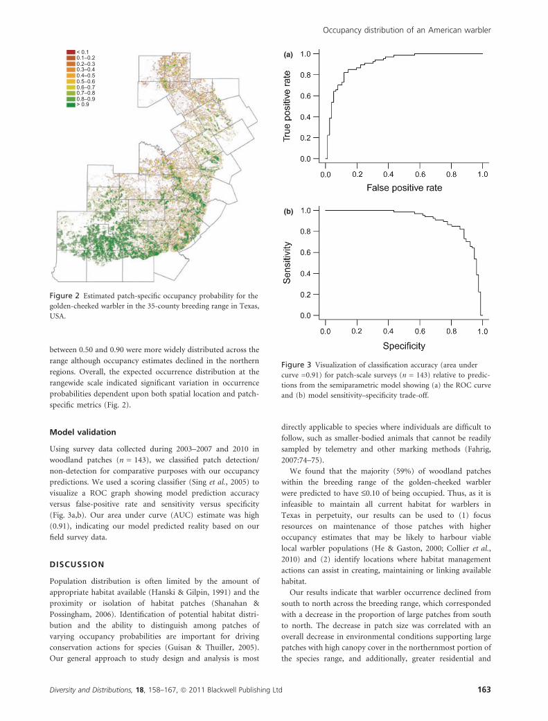
between 0.50 and 0.90 were more widely distributed across the

range although occupancy estimates declined in the northern

regions. Overall, the expected occurrence distribution at the

rangewide scale indicated significant variation in occurrence

probabilities dependent upon both spatial location and patch-

specific metrics (Fig. 2).

Model validation

Using survey data collected during 2003–2007 and 2010 in

woodland patches (n = 143), we classified patch detection/

non-detection for comparative purposes with our occupancy

predictions. We used a scoring classifier (Sing et al., 2005) to

visualize a ROC graph showing model prediction accuracy

versus false-positive rate and sensitivity versus specificity

(Fig. 3a,b). Our area under curve (AUC) estimate was high

(0.91), indicating our model predicted reality based on our

field survey data.

DISCUSSION

Population distribution is often limited by the amount of

appropriate habitat available (Hanski & Gilpin, 1991) and the

proximity or isolation of habitat patches (Shanahan &

Possingham, 2006). Identification of potential habitat distri-

bution and the ability to distinguish among patches of

varying occupancy probabilities are important for driving

conservation actions for species (Guisan & Thuiller, 2005).

Our general approach to study design and analysis is most

directly applicable to species where individuals are difficult to

follow, such as smaller-bodied animals that cannot be readily

sampled by telemetry and other marking methods (Fahrig,

2007:74–75).

We found that the majority (59%) of woodland patches

within the breeding range of the golden-cheeked warbler

were predicted to have £0.10 of being occupied. Thus, as it is

infeasible to maintain all current habitat for warblers in

Texas in perpetuity, our results can be used to (1) focus

resources on maintenance of those patches with higher

occupancy estimates that may be likely to harbour viable

local warbler populations (He & Gaston, 2000; Collier et al.,

2010) and (2) identify locations where habitat management

actions can assist in creating, maintaining or linking available

habitat.

Our results indicate that warbler occurrence declined from

south to north across the breeding range, which corresponded

with a decrease in the proportion of large patches from south

to north. The decrease in patch size was correlated with an

overall decrease in environmental conditions supporting large

patches with high canopy cover in the northernmost portion of

the species range, and additionally, greater residential and

< 0.10.1–0.20.2–0.30.3–0.40.4–0.50.5–0.60.6–0.70.7–0.80.8–0.9> 0.9

Figure 2 Estimated patch-specific occupancy probability for the

golden-cheeked warbler in the 35-county breeding range in Texas,

USA.

(a)

(b)

Figure 3 Visualization of classification accuracy (area under

curve =0.91) for patch-scale surveys (n = 143) relative to predic-

tions from the semiparametric model showing (a) the ROC curve

and (b) model sensitivity–specificity trade-off.

Occupancy distribution of an American warbler

Diversity and Distributions, 18, 158–167, ª 2011 Blackwell Publishing Ltd 163

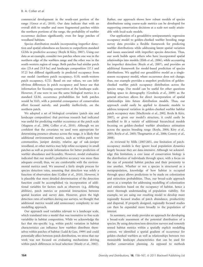
commercial development in the south-east portion of the

range (Groce et al., 2010). Our data indicate that with an

overall shift to smaller and more fragmented patches within

the northern portions of the range, the probability of warbler

occurrence declines significantly, even for large patches of

woodland habitats.

Species distribution models incorporating imperfect detec-

tion and spatial relatedness are known to outperform standard

GLMs in predictive accuracy (Royle & Kery, 2007). Using our

data as an example, consider two patches where one was in the

northern edge of the warblers range and the other was in the

south-western region of range. Both patches had similar patch

size (25.4 and 25.9 ha) and landscape composition (57.1 and

57.2) but differed significantly in predicted occupancy from

our model (northern patch occupancy, 0.10; south-western

patch occupancy, 0.72). Based on our values, we can infer

obvious differences in patch occupancy and hence use that

information for focusing conservation at the landscape scale.

However, if one were to use the same biological metrics in a

standard GLM, occurrence probabilities for both patches

would be 0.63, with a potential consequence of conservation

effort focused naıvely, and possibly ineffectively, on the

northern patch.

We adopted a set of biological covariates (patch size and

landscape composition) that previous research had indicated

was useful for predicting warbler occurrence at the patch scale

(Magness et al., 2006; Collier et al., 2010). Although we are

confident that the covariates we used were appropriate for

determining presence–absence across the range, it is likely that

additional environmental metrics, such as within-patch tree

communities, juniper density, relative age of oak–juniper

woodland, or other metrics may help refine occupancy in small

patches as well as provide information for better prediction of

warbler abundance and fecundity. However, model evaluation

indicated that our model’s predictive accuracy was more than

adequate overall; thus, we are comfortable with the environ-

mental metrics used. We assumed a fairly simple process for

species detection rates, assuming that detection was solely a

function of observation date (Collier et al., 2010). However, it

is plausible that more detailed determination of the detection

function could be accomplished via incorporation of addi-

tional variables for factors such as observers (e.g. differing

abilities), patch metrics or potential interactions between

spatial location and survey date. However, given the high

detection rates of warblers during our surveys, we thought that

additional metrics would add unnecessary complexity to our

modelling approach.

Our approach used variables relevant to a landscape scale,

which translated into a model that was insensitive to fine-scale

variability in habitat composition. While we acknowledge the

fact that site-specific (e.g. within patch) variation in habitat

characteristics can influence how warblers distribute them-

selves within patches of habitat (Ladd & Gass, 1999) and could

potentially affect between-patch distribution, we stress that our

work was not focused on evaluating mechanisms driving

within-patch differences in local selection (Manly et al., 2002).

Rather, our approach shows how robust models of species

distributions using coarse-scale metrics can be developed for

supporting conservation decisions at a scale not easily attain-

able with local-scale models.

Our application of a geoadditive semiparametric regression

occupancy model to golden-cheeked warbler breeding range

survey data provides a flexible framework for predicting

warbler distributions while addressing latent spatial variation

and issues associated with imperfect species detection. Thus,

our work builds upon others who have incorporated spatial

relationships into models (Elith et al., 2006), while accounting

for imperfect detection (Royle et al., 2007), and provides an

additional framework for model-based prediction of species

distributions. We applied our geoadditive model as a single-

season occupancy model, where occurrence does not change;

thus, our example provides a snapshot prediction of golden-

cheeked warbler patch occupancy distribution across the

species range. Our model can be useful for other questions

linking space to demography (Grosbois et al., 2009) as the

general structure allows for direct incorporation of spatial

relationships into future distribution models. Thus, our

approach could easily be applied to dynamic models to

address temporal variation in golden-cheeked warbler habitat

patch occupancy state (MacKenzie et al., 2002, Royle & Kery,

2007), or given our model’s structure, it could easily be

modified to fit a variety of additional hierarchical models

focusing on golden-cheeked warbler abundance estimation

across the species breeding range (Royle, 2004; Kery et al.,

2005; Royle et al., 2005; Thogmartin et al., 2006; Conroy et al.,

2008).

As reviewed by Mills (2007:265), one limitation of patch-

occupancy models is they ignore local population dynamics

largely because they are data-intensive. Although we acknowl-

edge this limitation, a core issue of conservation biology is

the distribution of individuals through space, with a focus on

the size of potential habitat patches and their proximity to

one another. Whether or not a species is structured as a

metapopulation, knowledge of how habitat is occupied

through space allows predictions to be made on colonization

and extinction probabilities. Thus, our broad-scale approach

serves as a template for addressing modelling of colonization

and extinction based on the occupancy of habitat, hence a

more thorough understanding of population viability. For

example, we are using our resulting model to develop more

regionally focused studies of patch abundance, productivity

and dispersal. If properly designed, regionally focused studies

can then be expanded more broadly to the population of

interest.

In summary, our study provides an approach for developing

a broad-scale assessment of the potential distribution of a

species. By using detection/non-detection surveys and remotely

sensed habitat metrics within a spatially explicit modelling

context, we identified a spatial gradient of occurrence for

golden-cheeked warblers as well as relationships between two

measurable landscape characteristics that can be used for

further conservation planning. As opposed to methods

B. A. Collier et al.

164 Diversity and Distributions, 18, 158–167, ª 2011 Blackwell Publishing Ltd

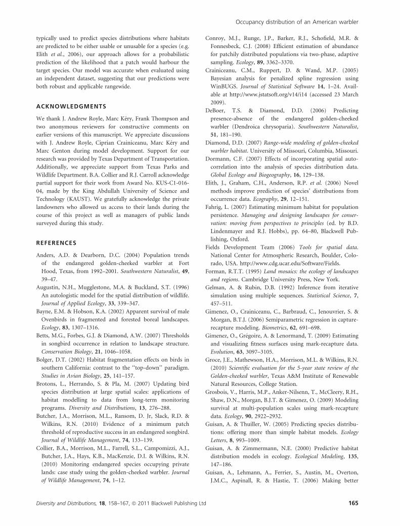
typically used to predict species distributions where habitats

are predicted to be either usable or unusable for a species (e.g.

Elith et al., 2006), our approach allows for a probabilistic

prediction of the likelihood that a patch would harbour the

target species. Our model was accurate when evaluated using

an independent dataset, suggesting that our predictions were

both robust and applicable rangewide.

ACKNOWLEDGMENTS

We thank J. Andrew Royle, Marc Kery, Frank Thompson and

two anonymous reviewers for constructive comments on

earlier versions of this manuscript. We appreciate discussions

with J. Andrew Royle, Ciprian Crainiceanu, Marc Kery and

Marc Genton during model development. Support for our

research was provided by Texas Department of Transportation.

Additionally, we appreciate support from Texas Parks and

Wildlife Department. B.A. Collier and R.J. Carroll acknowledge

partial support for their work from Award No. KUS-C1-016-

04, made by the King Abdullah University of Science and

Technology (KAUST). We gratefully acknowledge the private

landowners who allowed us access to their lands during the

course of this project as well as managers of public lands

surveyed during this study.

REFERENCES

Anders, A.D. & Dearborn, D.C. (2004) Population trends

of the endangered golden-cheeked warbler at Fort

Hood, Texas, from 1992–2001. Southwestern Naturalist, 49,

39–47.

Augustin, N.H., Mugglestone, M.A. & Buckland, S.T. (1996)

An autologistic model for the spatial distribution of wildlife.

Journal of Applied Ecology, 33, 339–347.

Bayne, E.M. & Hobson, K.A. (2002) Apparent survival of male

Ovenbirds in fragmented and forested boreal landscapes.

Ecology, 83, 1307–1316.

Betts, M.G., Forbes, G.J. & Diamond, A.W. (2007) Thresholds

in songbird occurrence in relation to landscape structure.

Conservation Biology, 21, 1046–1058.

Bolger, D.T. (2002) Habitat fragmentation effects on birds in

southern California: contrast to the ‘‘top-down’’ paradigm.

Studies in Avian Biology, 25, 141–157.

Brotons, L., Herrando, S. & Pla, M. (2007) Updating bird

species distribution at large spatial scales: applications of

habitat modelling to data from long-term monitoring

programs. Diversity and Distributions, 13, 276–288.

Butcher, J.A., Morrison, M.L., Ransom, D. Jr, Slack, R.D. &

Wilkins, R.N. (2010) Evidence of a minimum patch

threshold of reproductive success in an endangered songbird.

Journal of Wildlife Management, 74, 133–139.

Collier, B.A., Morrison, M.L., Farrell, S.L., Campomizzi, A.J.,

Butcher, J.A., Hays, K.B., MacKenzie, D.I. & Wilkins, R.N.

(2010) Monitoring endangered species occupying private

lands: case study using the golden-cheeked warbler. Journal

of Wildlife Management, 74, 1–12.

Conroy, M.J., Runge, J.P., Barker, R.J., Schofield, M.R. &

Fonnesbeck, C.J. (2008) Efficient estimation of abundance

for patchily distributed populations via two-phase, adaptive

sampling. Ecology, 89, 3362–3370.

Crainiceanu, C.M., Ruppert, D. & Wand, M.P. (2005)

Bayesian analysis for penalized spline regression using

WinBUGS. Journal of Statistical Software 14, 1–24. Avail-

able at http://www.jstatsoft.org/v14/i14 (accessed 23 March

2009).

DeBoer, T.S. & Diamond, D.D. (2006) Predicting

presence-absence of the endangered golden-cheeked

warbler (Dendroica chrysoparia). Southwestern Naturalist,

51, 181–190.

Diamond, D.D. (2007) Range-wide modeling of golden-cheeked

warbler habitat. University of Missouri, Columbia, Missouri.

Dormann, C.F. (2007) Effects of incorporating spatial auto-

correlation into the analysis of species distribution data.

Global Ecology and Biogeography, 16, 129–138.

Elith, J., Graham, C.H., Anderson, R.P. et al. (2006) Novel

methods improve prediction of species’ distributions from

occurrence data. Ecography, 29, 12–151.

Fahrig, L. (2007) Estimating minimum habitat for population

persistence. Managing and designing landscapes for conser-

vation: moving from perspectives to principles (ed. by B.D.

Lindenmayer and R.J. Hobbs), pp. 64–80, Blackwell Pub-

lishing, Oxford.

Fields Development Team (2006) Tools for spatial data.

National Center for Atmospheric Research, Boulder, Colo-

rado, USA. http://www.cdg.ucar.edu/Software/Fields.

Forman, R.T.T. (1995) Land mosaics: the ecology of landscapes

and regions. Cambridge University Press, New York.

Gelman, A. & Rubin, D.B. (1992) Inference from iterative

simulation using multiple sequences. Statistical Science, 7,

457–511.

Gimenez, O., Crainiceanu, C., Barbraud, C., Jenouvrier, S. &

Morgan, B.T.J. (2006) Semiparametric regression in capture-

recapture modeling. Biometrics, 62, 691–698.

Gimenez, O., Gregoire, A. & Lenormand, T. (2009) Estimating

and visualizing fitness surfaces using mark-recapture data.

Evolution, 63, 3097–3105.

Groce, J.E., Mathewson, H.A., Morrison, M.L. & Wilkins, R.N.

(2010) Scientific evaluation for the 5-year state review of the

Golden-cheeked warbler, Texas A&M Institute of Renewable

Natural Resources, College Station.

Grosbois, V., Harris, M.P., Anker-Nilsenn, T., McCleery, R.H.,

Shaw, D.N., Morgan, B.J.T. & Gimenez, O. (2009) Modeling

survival at multi-population scales using mark-recapture

data. Ecology, 90, 2922–2932.

Guisan, A. & Thuiller, W. (2005) Predicting species distribu-

tions: offering more than simple habitat models. Ecology

Letters, 8, 993–1009.

Guisan, A. & Zimmermann, N.E. (2000) Predictive habitat

distribution models in ecology. Ecological Modeling, 135,

147–186.

Guisan, A., Lehmann, A., Ferrier, S., Austin, M., Overton,

J.M.C., Aspinall, R. & Hastie, T. (2006) Making better

Occupancy distribution of an American warbler

Diversity and Distributions, 18, 158–167, ª 2011 Blackwell Publishing Ltd 165

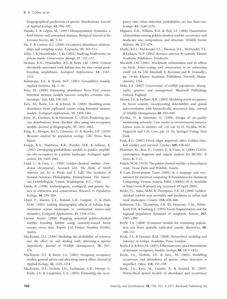
biogeographical predictions of species’ distributions. Journal

of Applied Ecology, 43, 386–392.

Hanski, I. & Gilpin, M. (1991) Metapopulation dynamics: a

brief history and conceptual domain. Biological Journal of the

Linnean Society, 42, 3–16.

He, F. & Gaston, K.J. (2000) Occupancy-abundance relation-

ships and sampling scales. Ecography, 23, 503–511.

Hilty, J. & Merenlender, A.M. (2003) Studying biodiversity on

private lands. Conservation Biology, 17, 132–137.

Homan, R.N., Windmiller, B.S. & Reed, J.M. (2004) Critical

thresholds associated with habitat loss for two vernal pool-

breeding amphibians. Ecological Applications, 14, 1547–

1553.

Kammann, E.E. & Wand, M.P. (2003) Geoadditive models.

Applied Statistics, 52, 1–18.

Kery, M. (2008) Estimating abundance form bird counts:

binomial mixture models uncover complex covariate rela-

tionships. Auk, 125, 336–345.

Kery, M., Royle, J.A. & Schmid, H. (2005) Modeling avian

abundance from replicated counts using binomial mixture

models. Ecological Applications, 15, 1450–1461.

Kery, M., Gardner, B. & Monnerat, C. (2010) Predicting spe-

cies distributions from checklist data using site-occupancy

models. Journal of Biogeography, 37, 1851–1862.

King, R., Morgan, B.J.T., Gimenez, O. & Brooks, S.P. (2010)

Bayesian analysis for population ecology. CRC Press, Boca

Raton.

Knapp, R.A., Matthews, K.R., Preisler, H.K. & Jellison, R.

(2003) Developing probabilistic models to predict amphib-

ian site occupancy in a patchy landscape. Ecological Appli-

cations, 13, 1069–1082.

Ladd, C. & Gass, L. (1999) Golden-cheeked warbler (Den-

droica chrysoparia). Account 420. The Birds of North

America (ed. by A. Poole and F. Gill) The Academy of

Natural Sciences, Philadelphia, Pennsylvania, The Ameri-

can Ornithologists’ Union, Washington, D.C., USA.

Lande, R. (1998) Anthropogenic, ecological, and genetic fac-

tors in extinction and conservation. Research in Population

Ecology, 40, 259–269.

Lloyd, P., Martin, T.E., Roland, L.R., Langner, U. & Hart,

M.M. (2005) Linking demographic effects of habitat frag-

mentation across landscapes to continental source-sink

dynamics. Ecological Applications, 15, 1504–1514.

Loomis Austin (2008) Mapping potential golden-cheeked

warbler breeding habitat using remotely-sensed forest

canopy cover data. Report LAI Project Number 051001,

Austin.

MacKenzie, D.I. (2006) Modeling the probability of resource

use: the effect of, and dealing with, detecting a species

imperfectly. Journal of Wildlife Management, 70, 367–

374.

MacKenzie, D.I. & Royle, J.A. (2005) Designing occupancy

studies: general advice and allocating survey effort. Journal of

Applied Ecology, 42, 1105–1114.

MacKenzie, D.I., Nichols, J.D., Lachmann, G.B., Droege, S.,

Royle, J.A. & Langtimm, C.A. (2002) Estimating site occu-

pancy rates when detection probabilities are less than one.

Ecology, 83, 2248–2255.

Magness, D.R., Wilkins, R.N. & Hejl, S.J. (2006) Quantitative

relationships among golden-cheeked warbler occurrence and

landscape size, composition, and structure. Wildlife Society

Bulletin, 34, 473–479.

Manly, B.F.J., McDonald, L.L., Thomas, D.L., McDonald, T.L.

& Erikson, W.P. (2002) Resource selection by animals. Kluwer

Academic Publishers, Dordrecht.

Marzluff, J.M. (2001) Worldwide urbanization and its effects

on birds. Avian ecology and conservation in an urbanizing

world (ed. by J.M. Marzluff, R. Bowman and R. Donnelly),

pp. 19–48, Kluwer Academic Publishers, Norwell, Massa-

chusetts, USA.

Mills, L.S. (2007) Conservation of wildlife populations: demog-

raphy, genetics, and management. Blackwell Publishing,

Oxford, England.

Moore, J.E. & Swihart, R.K. (2005) Modeling patch occupancy

by forest rodents: incorporating detectability and spatial

autocorrelation with hierarchically structured data. Journal

of Wildlife Management, 69, 933–949.

Nychka, D. & Saltzman, N. (1998) Design of air-quality

monitoring networks. Case studies in environmental statistics.

Lecture notes in statistics vol. 132 (ed. by D. Nychka, W.W.

Piegorsch and L.H. Cox), pp. 51–76, Springer-Verlag, New

York.

Peak, R.G. (2007) Forest edges negatively affect Golden-chee-

ked warbler nest survival. Condor, 109, 628–637.

Plummer, M., Best, N., Cowles, K. & Vines, K. (2006) CODA:

convergence diagnosis and output analysis for MCMC. R

News, 6, 7–11.

Pulich, W.M. (1976) The golden-cheeked warbler: a bioecological

study. Texas Parks and Wildlife, Austin.

R Core Development Team (2009) R: a language and envi-

ronment for statistical computing. R Foundation for Statistical

Computing, Vienna, Austria. ISBN 3-900051-07-0, Available

at http://www.R-project.org (accessed 19 April 2009).

Reidy, J.L., Stake, M.M. & Thompson, F.R. III (2008) Golden-

cheeked warbler nest mortality and predators in urban and

rural landscapes. Condor, 110, 458–466.

Robinson, S.K., Thompson, F.R. III, Donovan, T.M., White-

head, D.R. & Faaborg, J. (1995) Forest fragmentation and the

regional population dynamics of songbirds. Science, 267,

1987–1990.

Royle, J.A. (2004) N-mixture models for estimating popula-

tion size from spatially replicated counts. Biometrics, 60,

108–115.

Royle, J.A. & Dorazio, R.M. (2008) Hierarchical modeling and

inference in ecology. Academic Press, London.

Royle, J.A. & Kery, M. (2007) A Bayesian state-space formulation

of dynamic occupancy models. Ecology, 88, 1813–1823.

Royle, J.A., Nichols, J.D. & Kery, M. (2005) Modelling

occurrence and abundance of species when detection is

imperfect. Oikos, 110, 353–359.

Royle, J.A., Kery, M., Gautier, R. & Schmid, H. (2007)

Hierarchical spatial models of abundance and occurrence

B. A. Collier et al.

166 Diversity and Distributions, 18, 158–167, ª 2011 Blackwell Publishing Ltd

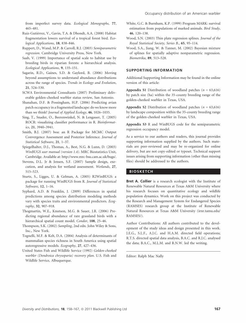
from imperfect survey data. Ecological Monographs, 77,

465–481.

Ruiz-Gutierrez, V., Gavin, T.A. & Dhondt, A.A. (2008) Habitat

fragmentation lowers survival of a tropical forest bird. Eco-

logical Applications, 18, 838–846.

Ruppert, D., Wand, M.P. & Carroll, R.J. (2003) Semiparametric

regression. Cambridge University Press, New York.

Saab, V. (1999) Importance of spatial scale to habitat use by

breeding birds in riparian forests: a hierarchical analysis.

Ecological Applications, 9, 135–151.

Sagarin, R.D., Gaines, S.D. & Gaylord, B. (2006) Moving

beyond assumptions to understand abundance distributions

across the range of species. Trends in Ecology and Evolution,

21, 524–530.

SCWA Environmental Consultants (2007) Preliminary deliv-

erable golden-cheeked warbler status review, San Antonio.

Shanahan, D.F. & Possingham, H.P. (2006) Predicting avian

patch occupancy in a fragmented landscape: do we know more

than we think? Journal of Applied Ecology, 46, 1026–1035.

Sing, T., Snader, O., Beerenwinkel, N. & Lengauer, T. (2005)

ROCR: visualizing classifier performance in R. Bioinformat-

ics, 21, 3940–3941.

Smith, B.J. (2007) boa: an R Package for MCMC Output

Convergence Assessment and Posterior Inference. Journal of

Statistical Software, 21, 1–37.

Spiegelhalter, D.J., Thomas, A., Best, N.G. & Lunn, D. (2003)

WinBUGS user manual (version 1.4). MRC Biostatistics Unit,

Cambridge. Available at: http://www.mrc-bsu.cam.ac.uk/bugs/.

Stevens, D.L. Jr & Jensen, S.F. (2007) Sample design, exe-

cution, and analysis for wetland assessment. Wetlands, 27,

515–523.

Sturtz, S., Ligges, U. & Gelman, A. (2005) R2WinBUGS: a

package for running WinBUGS from R. Journal of Statistical

Software, 12, 1–16.

Syphard, A.D. & Franklin, J. (2009) Differences in spatial

predictions among species distribution modeling methods

vary with species traits and environmental predictors. Ecog-

raphy, 32, 907–918.

Thogmartin, W.E., Knutson, M.G. & Sauer, J.R. (2006) Pre-

dicting regional abundance of rare grassland birds with a

hierarchical spatial count model. Condor, 108, 25–46.

Thompson, S.K. (2002) Sampling, 2nd edn. John Wiley & Sons,

Inc., New York.

Tognelli, M.F. & Kelt, D.A. (2004) Analysis of determinants of

mammalian species richness in South America using spatial

autoregressive models. Ecography, 27, 427–436.

United States Fish and Wildlife Service (1992) Golden-cheeked

warbler (Dendroica chrysoparia) recovery plan. U.S. Fish and

Wildlife Service, Albuquerque.

White, G.C. & Burnham, K.P. (1999) Program MARK: survival

estimation from populations of marked animals. Bird Study,

46, 120–138.

Wood, S.N. (2003) Thin plate regression splines. Journal of the

Royal Statistical Society, Series B., 65, 95–114.

Wood, S.A., Jiang, W. & Tanner, M. (2002) Bayesian mixture

of splines for spatially adaptive nonparametric regression.

Biometrika, 89, 513–528.

SUPPORTING INFORMATION

Additional Supporting Information may be found in the online

version of this article:

Appendix S1 Distribution of woodland patches (n = 63,616)

by patch size (ha) within the 35-county breeding range of the

golden-cheeked warbler in Texas, USA.

Appendix S2 Distribution of woodland patches (n = 63,616)

by landscape composition within the 35-county breeding range

of the golden-cheeked warbler in Texas, USA.

Appendix S3 R and WinBUGS code for the semiparametric

regression occupancy model.

As a service to our authors and readers, this journal provides

supporting information supplied by the authors. Such mate-

rials are peer-reviewed and may be re-organized for online

delivery, but are not copy-edited or typeset. Technical support

issues arising from supporting information (other than missing

files) should be addressed to the authors.

BIOSKETCH

Bret A. Collier is a research ecologist with the Institute of

Renewable Natural Resources at Texas A&M University where

his research focuses on quantitative ecology and wildlife

population dynamics. Work on this project was conducted by

the Research and Management System for Endangered Species

(RAMSES) research group at the Institute of Renewable

Natural Resources at Texas A&M University (irnr.tamu.edu/

RAMSES/).

Author Contributions: All authors contributed to the devel-

opment of the study ideas and design presented in this work.

J.E.G., S.L.F., A.J.C. and H.A.M. directed field operations;

R.T.S. directed spatial data analysis, B.A.C. and R.J.C. analysed

the data; B.A.C., M.L.M. and R.N.W. led the writing.

Editor: Ralph Mac Nally

Occupancy distribution of an American warbler

Diversity and Distributions, 18, 158–167, ª 2011 Blackwell Publishing Ltd 167

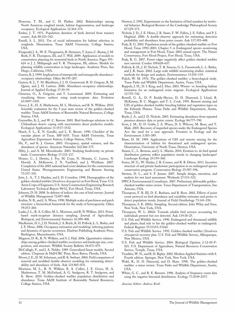
Donovan, T. M., and C. H. Flather. 2002. Relationships amongNorth American songbird trends, habitat fragmentation, and landscapeoccupancy. Ecological Applications 12:364–374.

Emlen, J. T. 1971. Population densities of birds derived from transectcounts. Auk 88:323–342.

Farrell, S. L. 2011. Use of social information for habitat selection insongbirds. Dissertation, Texas A&M University, College Station,USA.

Fitzgerald, J. A.,W. E. Thogmartin, R. Dettmers, T. Jones, C. Rustay, J. M.Ruth, F. R. Thompson, III, and T. Will. 2009. Application of models toconservation planning for terrestrial birds in North America. Pages 593–624 in J. J. Millspaugh and F. R. Thompson, III, editors. Models forplanning wildlife conservation in large landscapes. Academic Press, SanDiego, California, USA.

Gaston, K. J. 1999. Implications of interspecific and intraspecific abundance-occupancy relationships. Oikos 86:195–207.

Gaston, K. J., T. M. Blackburn, J. J. D. Greenwood, R. D. Gregory, R. M.Quinn, and J. H. Lawton. 2000. Abundance-occupancy relationships.Journal of Applied Ecology 37:39–59.

Gimenez, O., A. Gregoire, and T. Lenormand. 2009. Estimating andvisualizing fitness surfaces using mark-recapture data. Evolution63:3097–3105.

Groce, J. E., H. A. Mathewson, M. L. Morrison, and R. N. Wilkins. 2010.Scientific evaluation for the 5-year state review of the golden-cheekedwarbler. Texas A&M Institute of Renewable Natural Resources, CollegeStation, USA.

Gutzwiller, K. J., and W. C. Barrow. 2001. Bird-landscape relations in theChihuahuan desert: coping with uncertainties about predictive models.Ecological Applications 11:1517–1532.

Hatch, S. L., K. N. Gandhi, and L. E. Brown. 1990. Checklist of thevascular plants of Texas. MP-1655. Texas A&M University, TexasAgriculture Experiment Station, College Station, USA.

He, F., and K. J. Gaston. 2003. Occupancy, spatial variance, and theabundance of species. American Naturalist 162:366–375.

Hilty, J., and A. M. Merenlender. 2003. Studying biodiversity on privatelands. Conservation Biology 17:132–137.

Homer, C., J. Dewitz, J. Fry, M. Coan, N. Hossain, C. Larson, N.Herold, A. McKerrow, J. N. VanDriel, and J. Wickham. 2007.Completion of the 2001 national land cover database for the conterminousUnited States. Photogrammetric Engineering and Remote Sensing73:337–341.

Jette, L. A., T. J. Hayden, and J. D. Cornelius. 1998. Demographics of thegolden-cheeked warbler (Dendroica chrysoparia) on FortHood, Texas. U.S.ArmyCorps of Engineers, U.S. ArmyConstruction Engineering ResearchLaboratory Technical Report 98/52, Fort Hood, Texas, USA.

Johnson, D. H. 2008. In defense of indices: the case of bird surveys. Journalof Wildlife Management 72:857–868.

Kotliar, N. B., and J. A.Wiens. 1990.Multiple scales of patchiness and patchstructure: a hierarchical framework for the study of heterogeneity. Oikos59:253–260.

Laake, J. L., B. A. Collier, M. L. Morrison, and R. N.Wilkins. 2011. Point-based mark-recapture distance sampling. Journal of Agricultural,Biological, and Environmental Statistics 16:389–408.

MacKenzie, D. I., J. D. Nichols, J. A. Royle, K. H. Pollock, L. L. Bailey, andJ. E. Hines. 2006. Occupancy estimation and modeling: inferring patternsand dynamics of species occurrence. Elselvier Publishing Academic Press,Burlington, Massachusetts, USA.

Magness, D. R., R. N. Wilkins, and S. J. Hejl. 2006. Quantitative relation-ships among golden-cheeked warbler occurrence and landscape size, com-position, and structure. Wildlife Society Bulletin 34:473–479.

McCullagh, P., and J. A. Nelder. 1989. Generalized linear models. Secondedition. Chapman & Hall/CRC Press, Boca Raton, Florida, USA.

Moore, J. E., D.M. Scheiman, and R. K. Swihart. 2004. Field comparison ofremoval and modified double-observer modeling for estimating detect-ability and abundance of birds. Auk 121:865–876.

Morrison, M. L., R. N. Wilkins, B. A. Collier, J. E. Groce, H. A.Mathewson, T. M. McFarland, A. G. Snelgrove, R. T. Snelgrove, andK. Skow. 2010. Golden-cheeked warbler population distribution andabundance. Texas A&M Institute of Renewable Natural Resources,College Station, USA.

Newton, I. 1992. Experiments on the limitation of bird numbers by territo-rial behavior. Biological Reviews of the Cambridge Philosophical Society67:129–173.

Nichols, J. D., J. E. Hines, J. R. Sauer, F. W. Fallon, J. E. Fallon, and P. J.Heglund. 2000. A double-observer approach for estimating detectionprobability and abundance from point counts. Auk 117:393–408.

Peak, R. G. 2003. Population trends of the golden-cheeked warbler on FortHood, Texas 1992–2003. Chapter 5 in Endangered species monitoringand management at Fort Hood, Texas: 2003 annual report. The NatureConservancy, Fort Hood Project, Fort Hood, Texas, USA.

Peak, R. G. 2007. Forest edges negatively affect golden-cheeked warblernest survival. Condor 109:628–637.

Pollock, K. H., J. D. Nichols, T. R. Simons, G. L. Farnsworth, L. L. Bailey,and J. R. Sauer. 2002. Large scale wildlife monitoring studies: statisticalmethods for design and analysis. Environmetrics 13:105–119.

Pulich, W. M. 1976. The golden-cheeked warbler: a bioecological study.Texas Parks and Wildlife Department, Austin, Texas, USA.

Rappole, J. H., D. I. King, and J. Diez. 2003. Winter- vs. breeding-habitatlimitation for an endangered avian migrant. Ecological Applications13:735–742.

Rowell, G. A., D. P. Keddy-Hector, D. D. Diamond, J. Lloyd, B.McKinney, R. C. Maggio, and T. L. Cook. 1995. Remote sensing andGIS of golden-cheeked warbler breeding habitat and vegetation types onthe Edwards Plateau. Texas Parks and Wildlife Department, Austin,Texas, USA.

Royle, J. A., and J. D. Nichols. 2003. Estimating abundance from repeatedpresence-absence data or point counts. Ecology 84:777–790.

Scott, J. M., D. D. Goble, J. A. Wiens, D. S. Wilcove, M. Bean, and T.Male. 2005. Recovery of imperiled species under the Endangered SpeciesAct: the need for a new approach. Frontiers in Ecology and theEnvironment 3:383–389.

Shaw, D. M. 1989. Applications of GIS and remote sensing for thecharacterization of habitat for threatened and endangered species.Dissertation, University of North Texas, Denton, USA.

Sirami, C., L. Brotons, and J.-L. Martin. 2010. Erratum to: do bird spatialdistribution patterns reflect population trends in changing landscapes?Landscape Ecology 25:159–160.

Sorice, M. G., W. Haider, J. R. Conner, and R. B. Ditton. 2011. Incentivestructure of and private landowner participation in an endangered speciesconservation program. Conservation Biology 25:587–596.

Stevens, D. L., and S. F. Jensen. 2007. Sample design, execution, andanalysis for wet land assessment. Wetlands 27:515–523.

SWCA Environmental Consultants. 2007. Preliminary deliverable golden-cheeked warbler status review. Texas Department of Transportation, SanAntonio, USA.

Thompson, F. R. III, D. E. Burhans, and B. Root. 2002. Effects of pointcount protocol on bird abundance and variability estimates and power todetect population trends. Journal of Field Ornithology 73:141–150.

Thompson, S. K. 2002a. Sampling. Second edition. John Wiley and Sons,New York, New York, USA.

Thompson, W. L. 2002b. Towards reliable bird surveys: accounting forindividuals present but not detected. Auk 119:18–25.

U.S. Fish and Wildlife Service. 1990. Endangered and threatened wildlifeand plants; final rule to list the golden-cheeked warbler as endangered.Federal Register 55:53153–53160.

U.S. Fish and Wildlife Service. 1992. Golden-cheeked warbler (Dendroicachrysoparia) recovery plan. U.S. Fish and Wildlife Service, Albuquerque,New Mexico, USA.

U.S. Fish and Wildlife Service. 2004. Biological Opinion 2-12-05-F-021. U.S. Department of Agriculture, Natural Resources ConservationService, Temple, Texas, USA.

Venables,W. N., and B. D. Ripley. 2002. Modern Applied Statistics with S.Fourth edition. Springer, New York, New York, USA.

Wahl, R., D. D. Diamond, and D. Shaw. 1990. The golden-cheekedwarbler: a status review. Texas Parks and Wildlife Department, Austin,USA.

White, G. C., and R. E. Bennets. 1996. Analysis of frequency count datausing the negative binomial distribution. Ecology 77:2549–2557.

Associate Editor: Andrew Kroll.

12 The Journal of Wildlife Management