Embed Size (px)
Citation preview

Text Databases
Outline
Spatial Databases Temporal Databases Spatio-temporal Databases Data Mining Multimedia Databases
Text databases Image and video databases Time Series databases
Text - Detailed outline
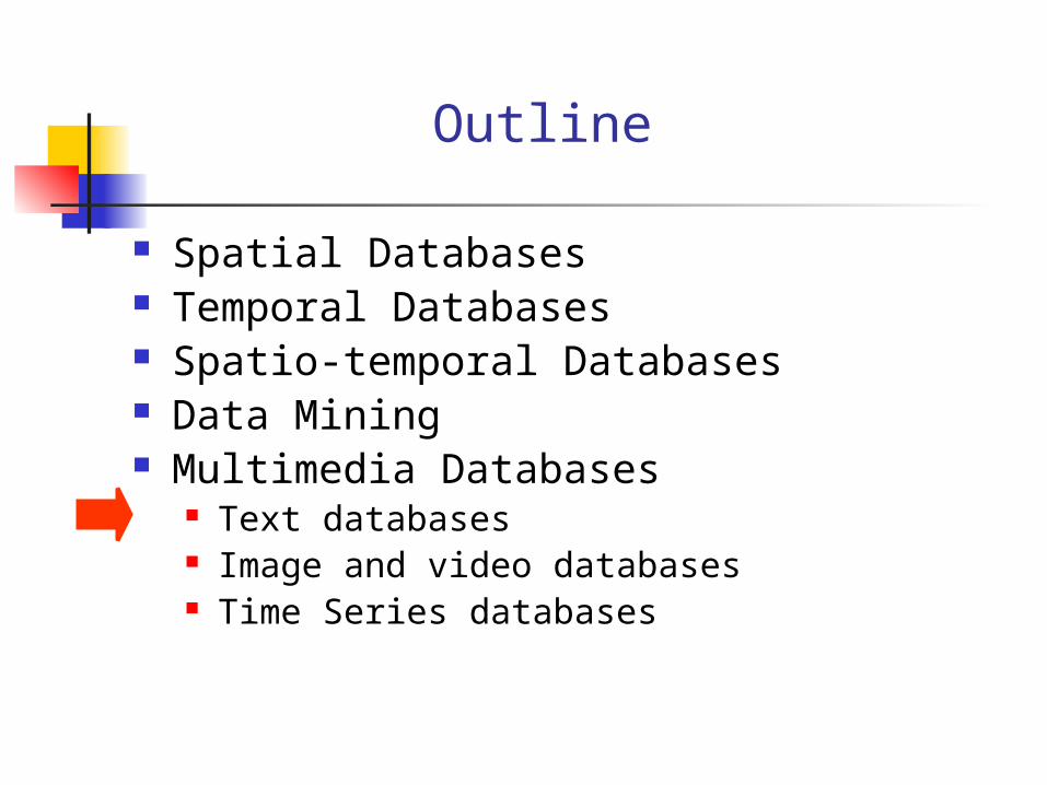
Text databases problem full text scanning inversion signature files (a.k.a. Bloom Filters) Vector model and clustering information filtering and LSI
Vector Space Model and Clustering
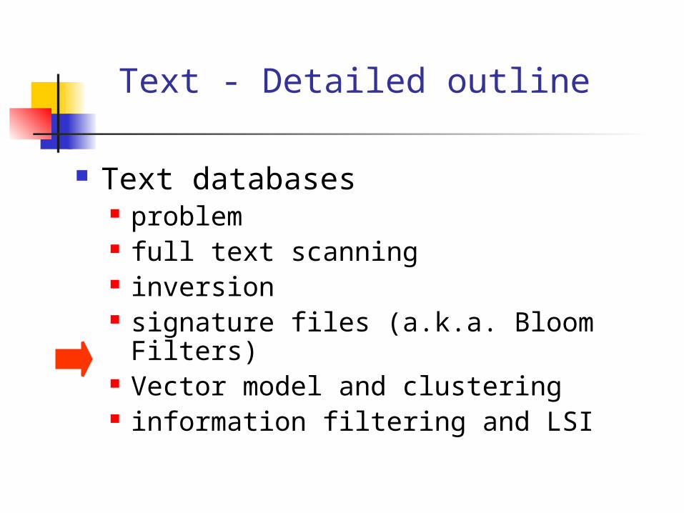
Keyword (free-text) queries (vs Boolean) each document: -> vector (HOW?) each query: -> vector search for ‘similar’ vectors
Vector Space Model and Clustering
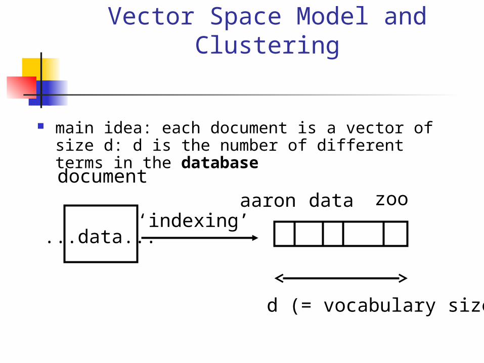
main idea: each document is a vector of size d: d is the number of different terms in the database
document
...data...
aaron zoodata
d (= vocabulary size)
‘indexing’
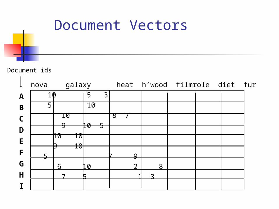
Document Vectors
Documents are represented as “bags of words”
Represented as vectors when used computationally A vector is like an array of floating points Has direction and magnitude Each vector holds a place for every term in the
collection Therefore, most vectors are sparse
Document VectorsOne location for each word.
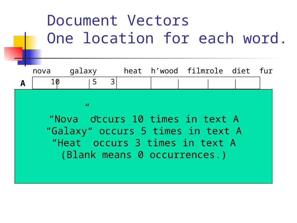
nova galaxy heat h’wood film rolediet fur
10 5 3 5 10
10 8 7 9 10 5
10 10 9 10
5 7 9 6 10 2 8
7 5 1 3
ABCDEFGHI
“Nova” occurs 10 times in text A“Galaxy” occurs 5 times in text A“Heat” occurs 3 times in text A(Blank means 0 occurrences.)
Document VectorsOne location for each word.
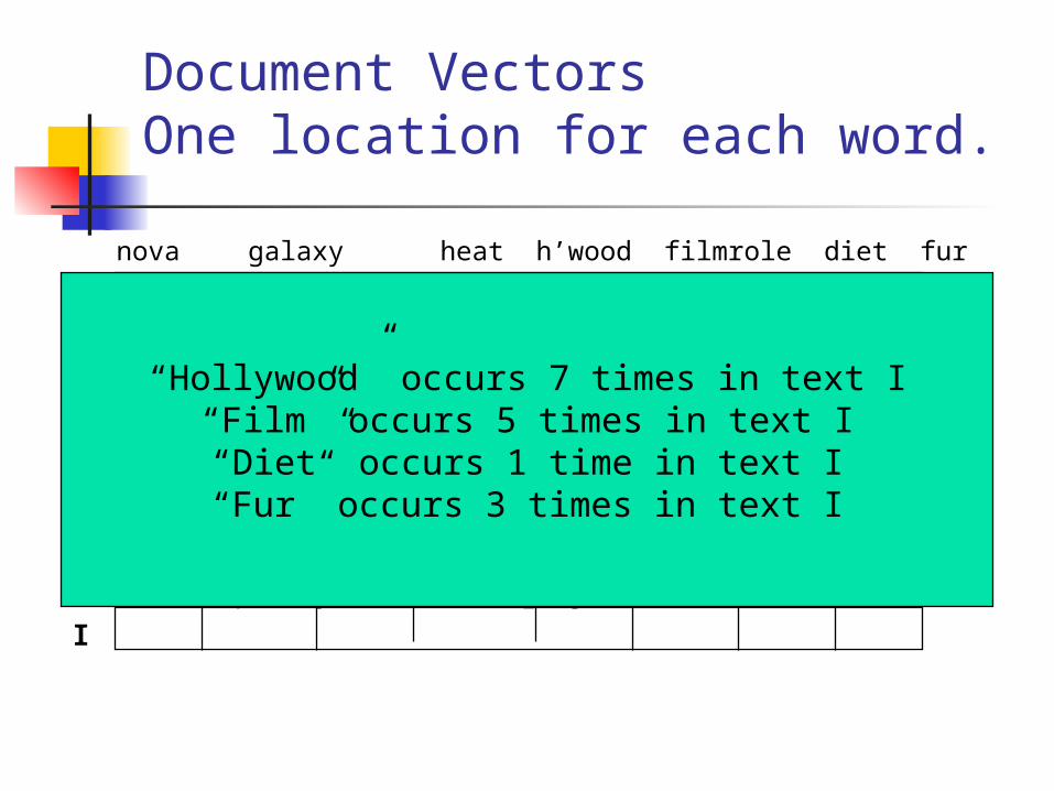
nova galaxy heat h’wood film rolediet fur
10 5 3 5 10
10 8 7 9 10 5
10 10 9 10
5 7 9 6 10 2 8
7 5 1 3
ABCDEFGHI
“Hollywood” occurs 7 times in text I“Film” occurs 5 times in text I“Diet” occurs 1 time in text I“Fur” occurs 3 times in text I
Document Vectors
nova galaxy heat h’wood film rolediet fur
10 5 3 5 10
10 8 7 9 10 5
10 10 9 10
5 7 9 6 10 2 8
7 5 1 3
ABCDEFGHI
Document ids
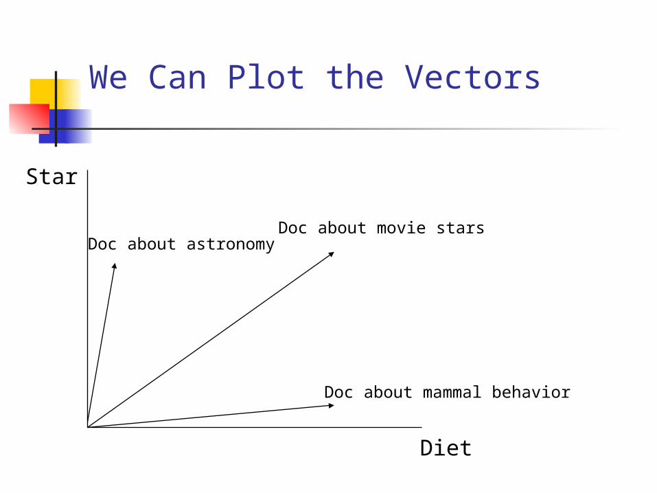
We Can Plot the Vectors
Star
Diet
Doc about astronomyDoc about movie stars
Doc about mammal behavior
Vector Space Model and Clustering
Then, group nearby vectors together Q1: cluster search? Q2: cluster generation?
Two significant contributions ranked output relevance feedback
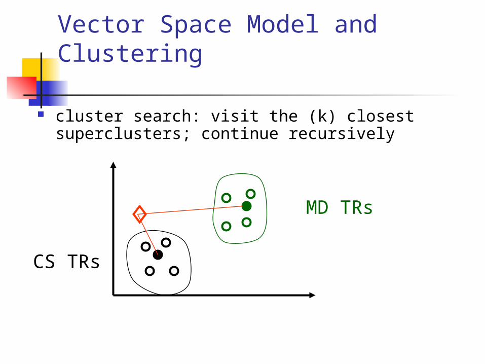
Vector Space Model and Clustering
cluster search: visit the (k) closest superclusters; continue recursively
CS TRs
MD TRs
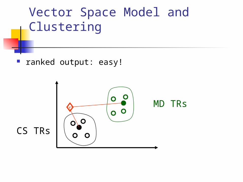
Vector Space Model and Clustering
ranked output: easy!
CS TRs
MD TRs
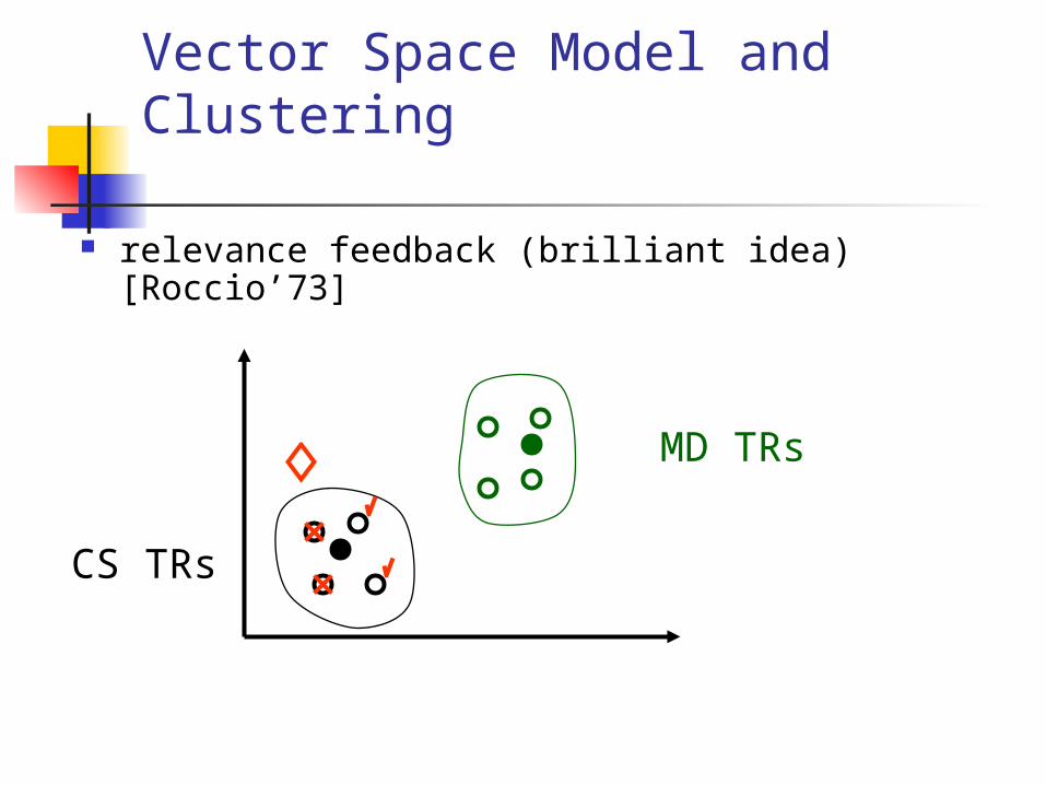
Vector Space Model and Clustering
relevance feedback (brilliant idea) [Roccio’73]
CS TRs
MD TRs
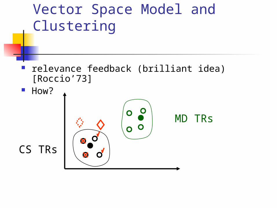
Vector Space Model and Clustering
relevance feedback (brilliant idea) [Roccio’73] How?
CS TRs
MD TRs
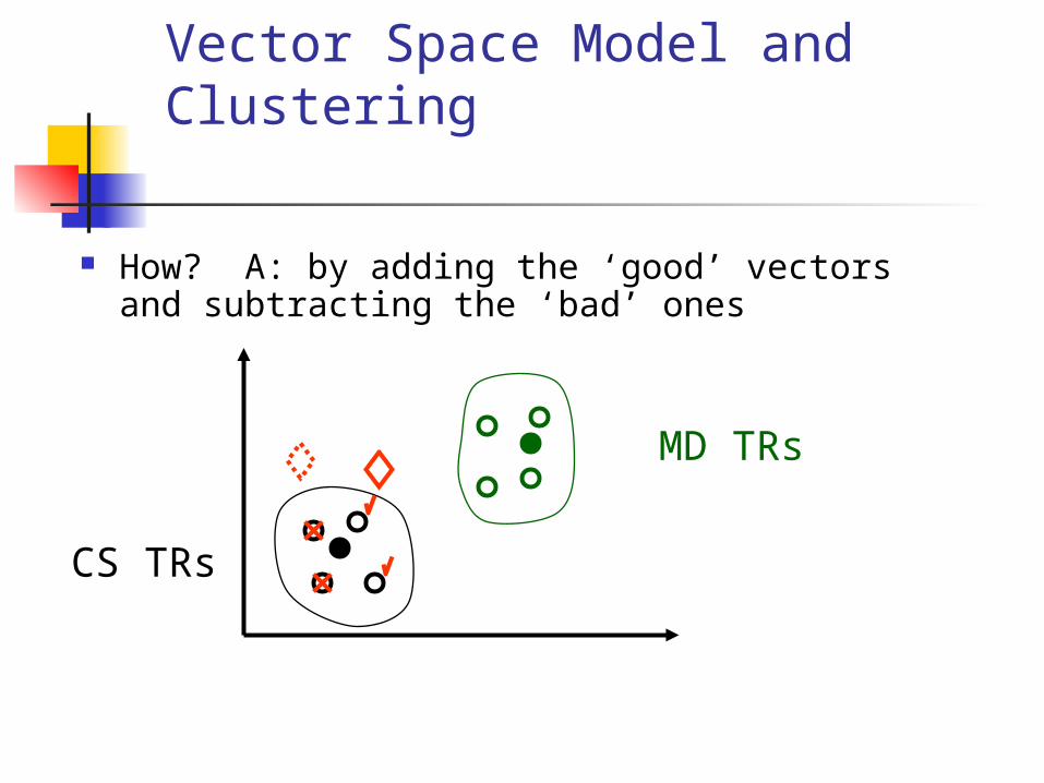
Vector Space Model and Clustering
How? A: by adding the ‘good’ vectors and subtracting the ‘bad’ ones
CS TRs
MD TRs
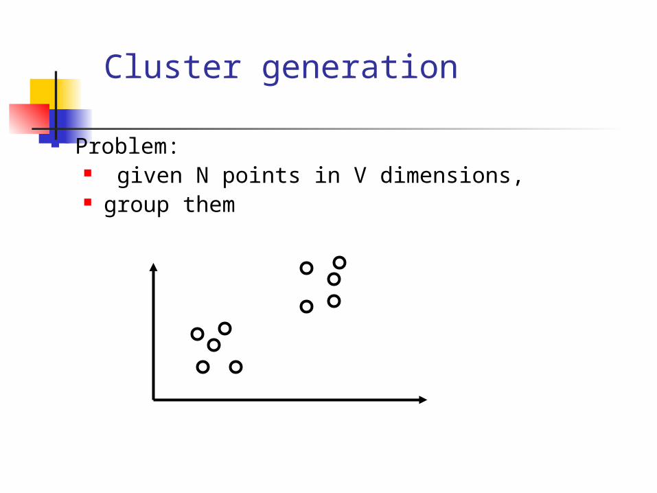
Cluster generation
Problem: given N points in V dimensions, group them
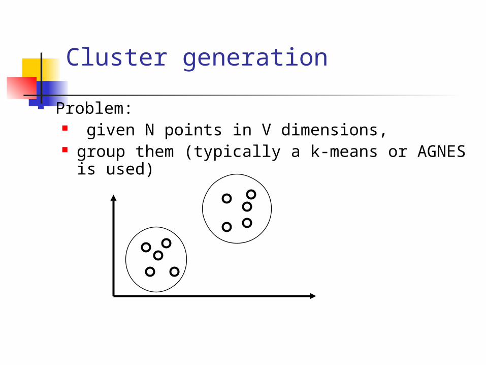
Cluster generation
Problem: given N points in V dimensions, group them (typically a k-means or AGNES is
used)
Assigning Weights to Terms
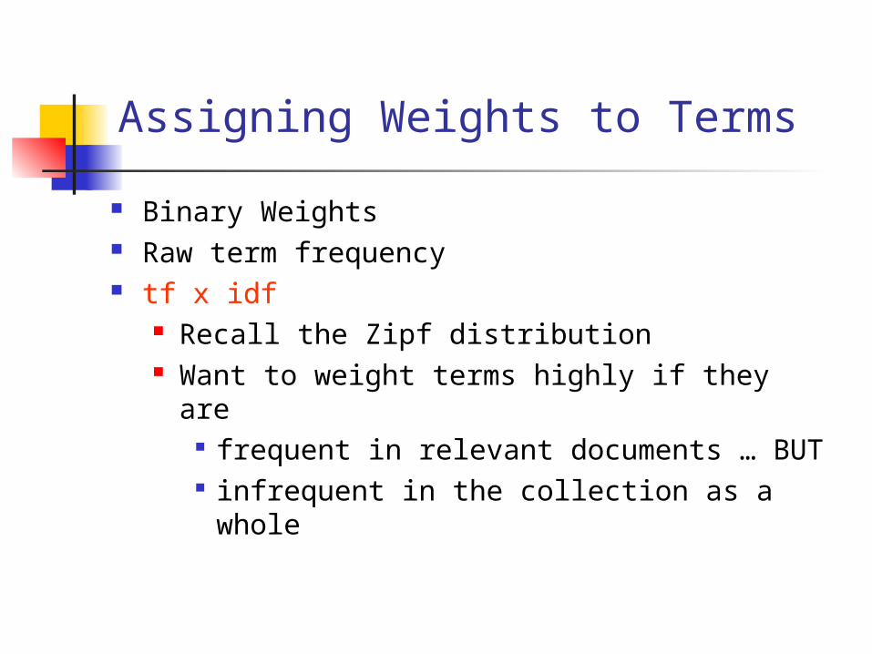
Binary Weights Raw term frequency tf x idf
Recall the Zipf distribution Want to weight terms highly if they are
frequent in relevant documents … BUT infrequent in the collection as a whole
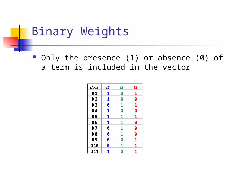
Binary Weights
Only the presence (1) or absence (0) of a term is included in the vector
docs t1 t2 t3D1 1 0 1D2 1 0 0D3 0 1 1D4 1 0 0D5 1 1 1D6 1 1 0D7 0 1 0D8 0 1 0D9 0 0 1D10 0 1 1D11 1 0 1
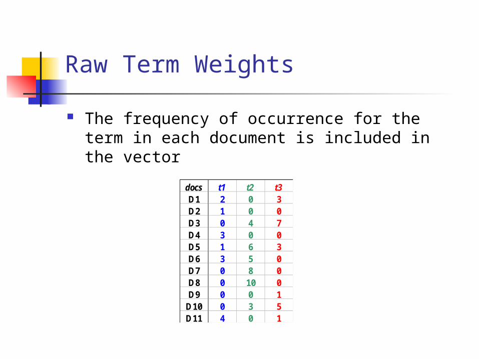
Raw Term Weights
The frequency of occurrence for the term in each document is included in the vector
docs t1 t2 t3D1 2 0 3D2 1 0 0D3 0 4 7D4 3 0 0D5 1 6 3D6 3 5 0D7 0 8 0D8 0 10 0D9 0 0 1D10 0 3 5D11 4 0 1
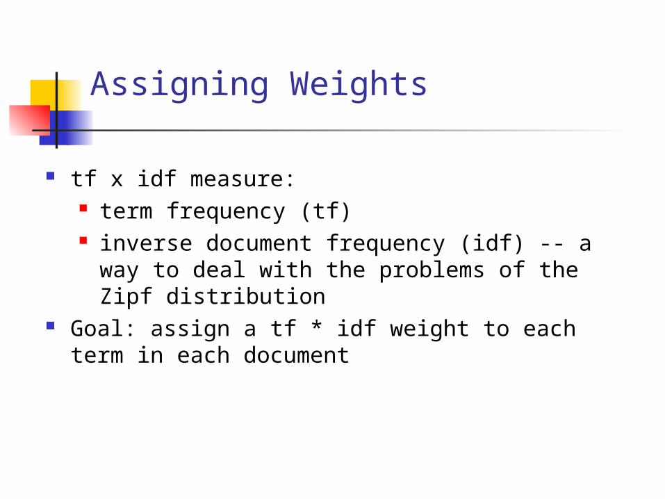
Assigning Weights
tf x idf measure: term frequency (tf) inverse document frequency (idf) -- a way to
deal with the problems of the Zipf distribution
Goal: assign a tf * idf weight to each term in each document
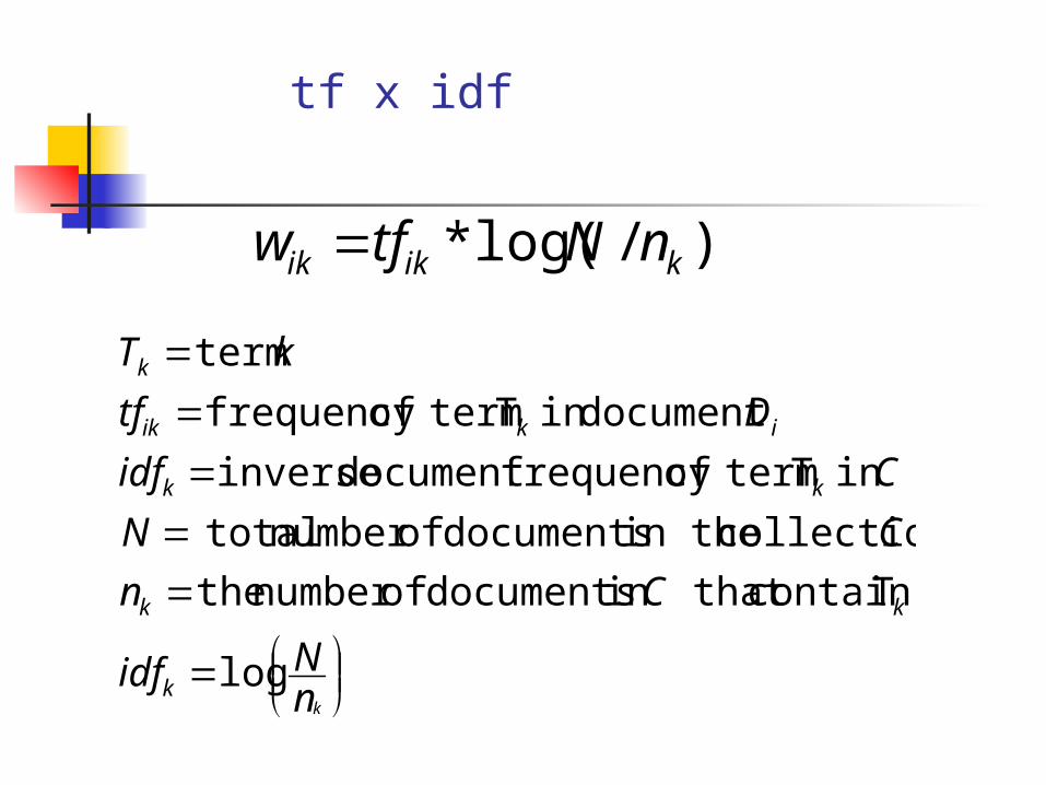
tf x idf
)/log(* kikik nNtfw
log
Tcontain that in documents ofnumber the
collection in the documents ofnumber total
in T termoffrequency document inverse
document in T termoffrequency
term
nNidf
Cn
CN
Cidf
Dtf
kT
kk
kk
kk
ikik
k
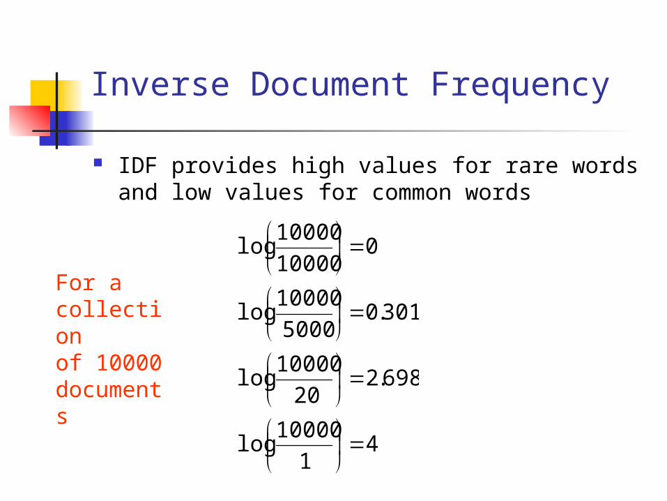
Inverse Document Frequency
IDF provides high values for rare words and low values for common words
41
10000log
698.220
10000log
301.05000
10000log
010000
10000log
For a collectionof 10000 documents
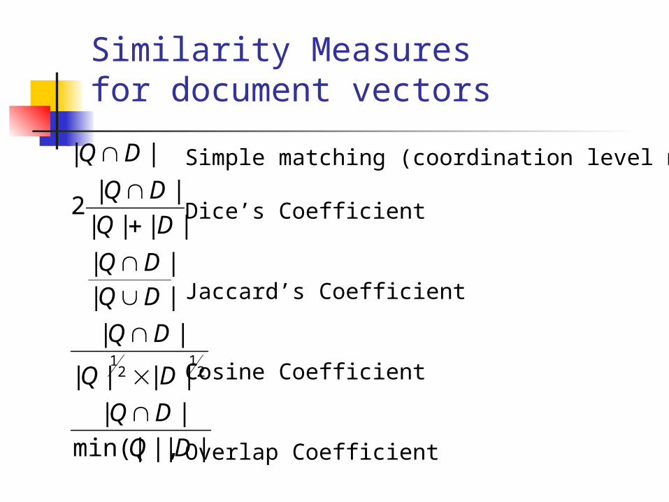
Similarity Measures for document vectors
|)||,min(|
||
||||
||
||||
||||
||2
||
21
21
DQ
DQ
DQ
DQ
DQDQ
DQ
DQ
DQ
Simple matching (coordination level match)
Dice’s Coefficient
Jaccard’s Coefficient
Cosine Coefficient
Overlap Coefficient
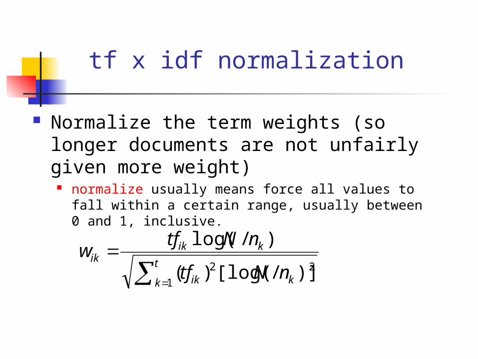
tf x idf normalization
Normalize the term weights (so longer documents are not unfairly given more weight)
normalize usually means force all values to fall within a certain range, usually between 0 and 1, inclusive.
t
k kik
kikik
nNtf
nNtfw
1
22 )]/[log()(
)/log(
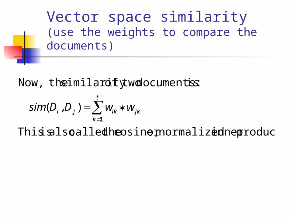
Vector space similarity(use the weights to compare the documents)
product.inner normalizedor cosine, thecalled also is This
),(
:is documents twoof similarity theNow,
1
t
kjkikji wwDDsim
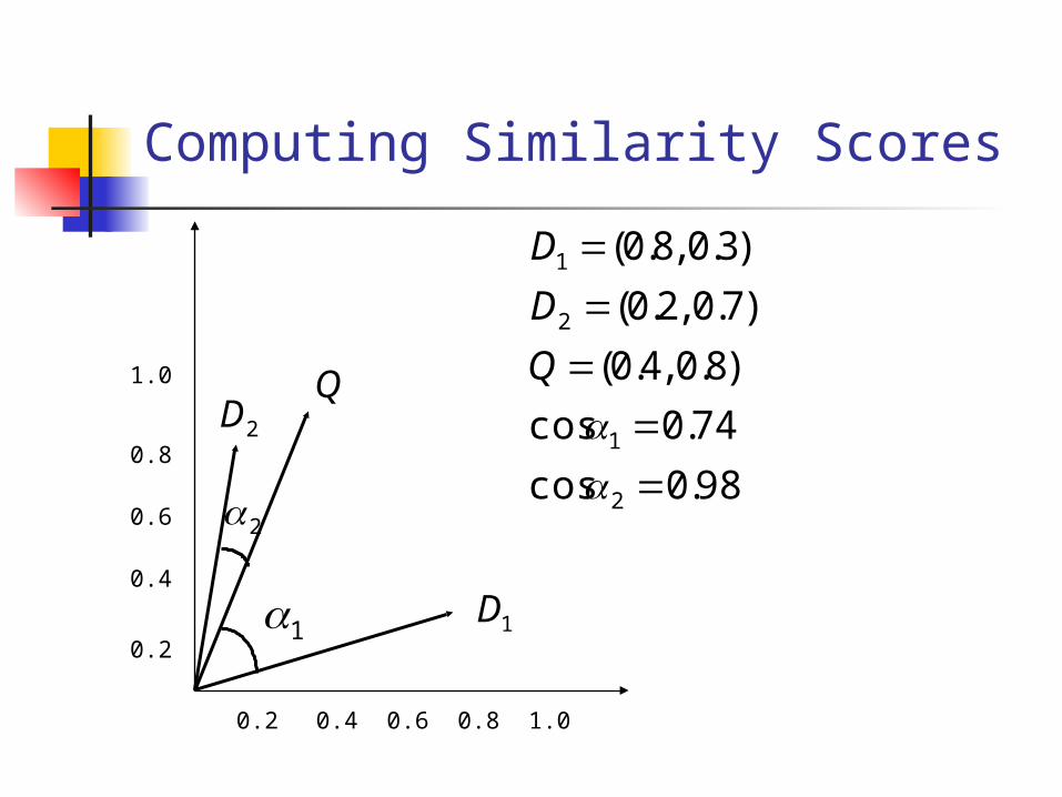
Computing Similarity Scores
2
1 1D
Q2D
98.0cos
74.0cos
)8.0 ,4.0(
)7.0 ,2.0(
)3.0 ,8.0(
2
1
2
1
Q
D
D
1.0
0.8
0.6
0.8
0.4
0.60.4 1.00.2
0.2
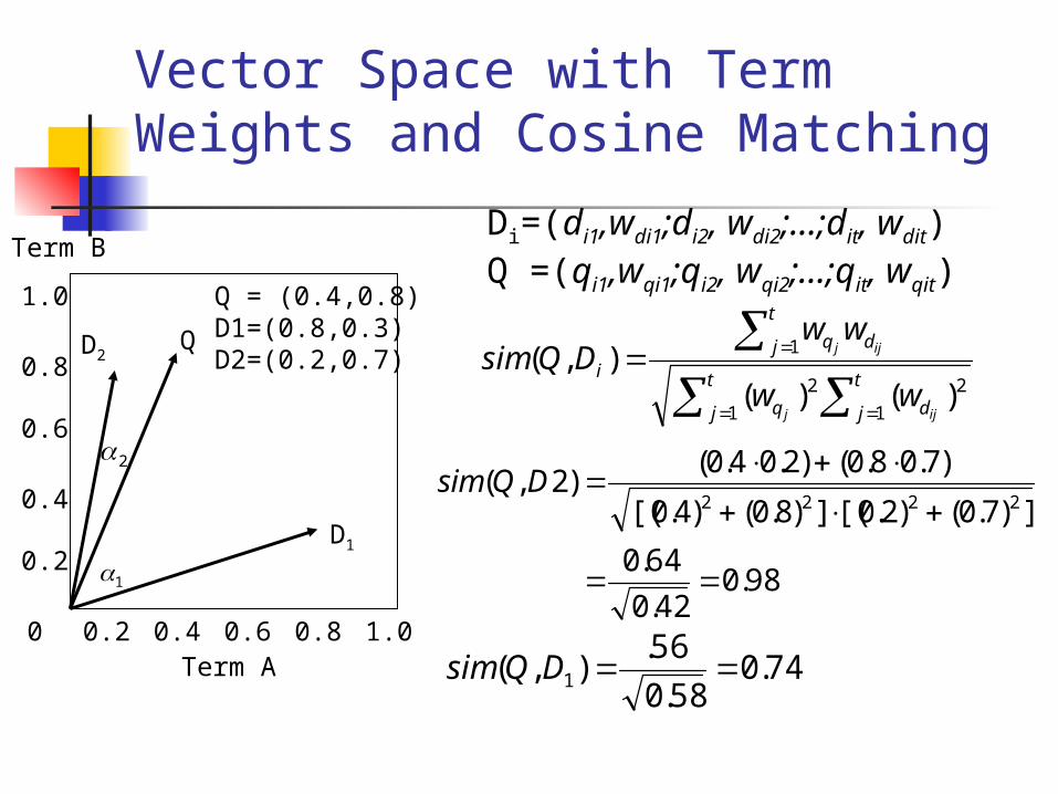
Vector Space with Term Weights and Cosine Matching
1.0
0.8
0.6
0.4
0.2
0.80.60.40.20 1.0
D2
D1
Q
1
2
Term B
Term A
Di=(di1,wdi1;di2, wdi2;…;dit, wdit)Q =(qi1,wqi1;qi2, wqi2;…;qit, wqit)
t
j
t
j dq
t
j dq
i
ijj
ijj
ww
wwDQsim
1 1
22
1
)()(),(
Q = (0.4,0.8)D1=(0.8,0.3)D2=(0.2,0.7)
98.042.0
64.0
])7.0()2.0[(])8.0()4.0[(
)7.08.0()2.04.0()2,(
2222
DQsim
74.058.0
56.),( 1 DQsim
Text - Detailed outline
Text databases problem full text scanning inversion signature files (a.k.a. Bloom Filters) Vector model and clustering information filtering and LSI
Information Filtering + LSI [Foltz+,’92] Goal:
users specify interests (= keywords) system alerts them, on suitable news-
documents Major contribution: LSI = Latent
Semantic Indexing latent (‘hidden’) concepts
Information Filtering + LSI
Main idea map each document into some
‘concepts’ map each term into some ‘concepts’
‘Concept’:~ a set of terms, with weights, e.g. “data” (0.8), “system” (0.5), “retrieval”
(0.6) -> DBMS_concept
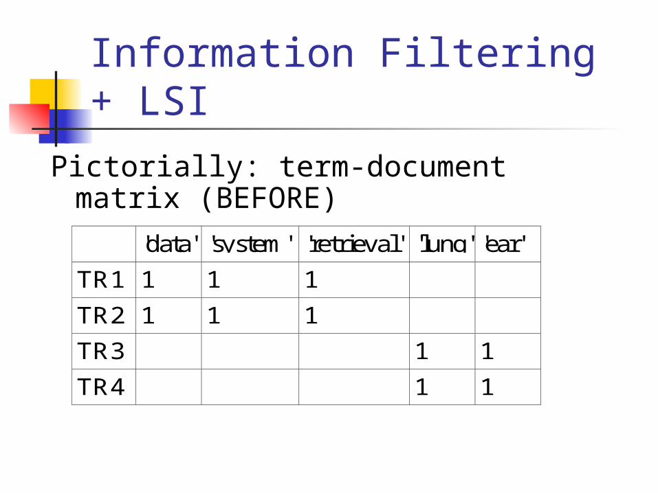
Information Filtering + LSI
Pictorially: term-document matrix (BEFORE)
'data' 'system' 'retrieval' 'lung' 'ear'
TR1 1 1 1
TR2 1 1 1
TR3 1 1
TR4 1 1
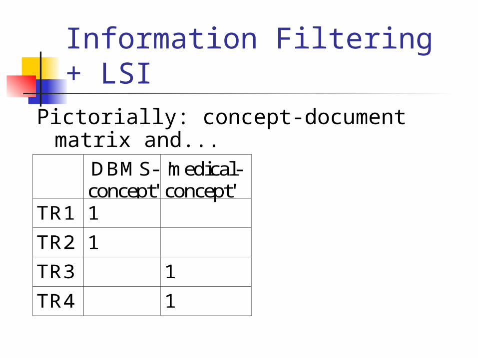
Information Filtering + LSIPictorially: concept-document matrix
and...'DBMS-concept'
'medical-concept'
TR1 1
TR2 1
TR3 1
TR4 1
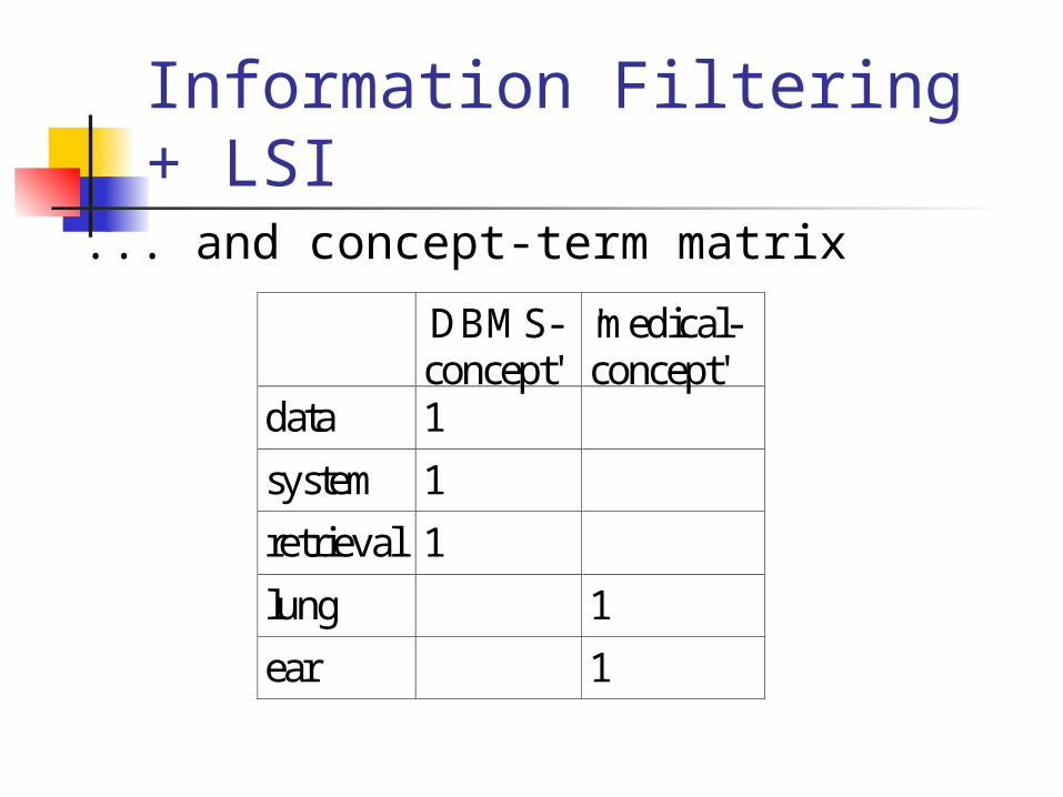
Information Filtering + LSI... and concept-term matrix
'DBMS-concept'
'medical-concept'
data 1
system 1
retrieval 1
lung 1
ear 1
Information Filtering + LSI
Q: How to search, eg., for ‘system’?
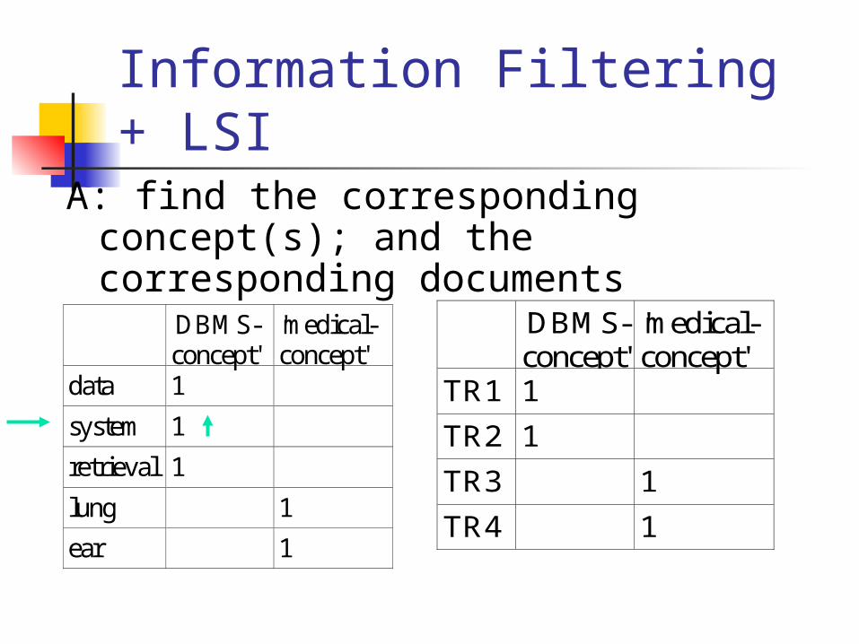
Information Filtering + LSIA: find the corresponding concept(s);
and the corresponding documents
'DBMS-concept'
'medical-concept'
data 1
system 1
retrieval 1
lung 1
ear 1
'DBMS-concept'
'medical-concept'
TR1 1
TR2 1
TR3 1
TR4 1
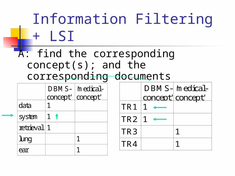
Information Filtering + LSIA: find the corresponding concept(s);
and the corresponding documents
'DBMS-concept'
'medical-concept'
data 1
system 1
retrieval 1
lung 1
ear 1
'DBMS-concept'
'medical-concept'
TR1 1
TR2 1
TR3 1
TR4 1
Information Filtering + LSI
Thus it works like an (automatically constructed) thesaurus:
we may retrieve documents that DON’T have the term ‘system’, but they contain almost everything else (‘data’, ‘retrieval’)
SVD - Detailed outline Motivation Definition - properties Interpretation Complexity Case studies Additional properties
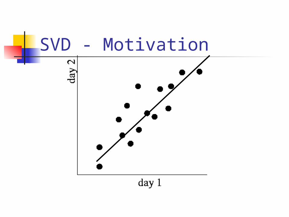
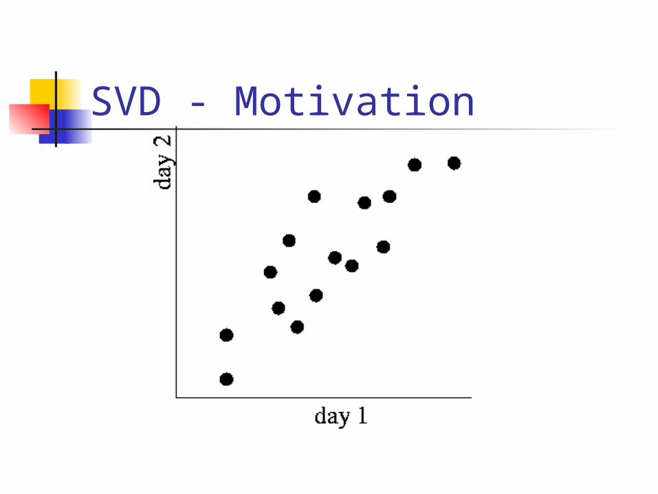
SVD - Motivation problem #1: text - LSI: find
‘concepts’ problem #2: compression / dim.
reduction
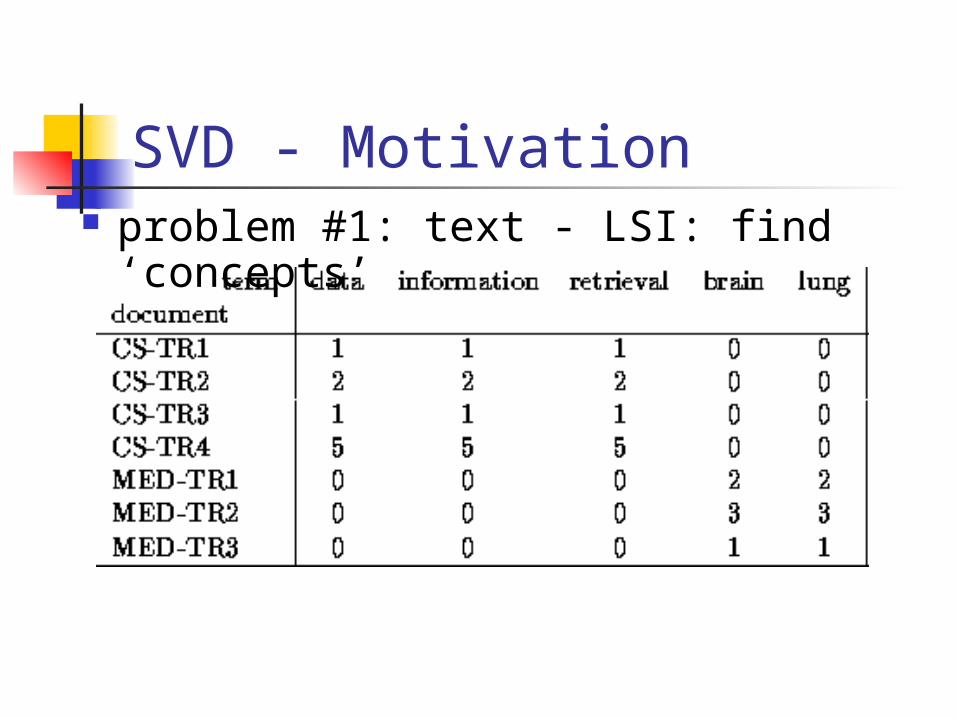
SVD - Motivation problem #1: text - LSI: find
‘concepts’
SVD - Motivation problem #2: compress / reduce
dimensionality
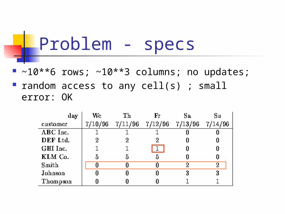
Problem - specs ~10**6 rows; ~10**3 columns; no updates; random access to any cell(s) ; small error: OK

SVD - Motivation
SVD - Motivation
SVD - Detailed outline Motivation Definition - properties Interpretation Complexity Case studies Additional properties
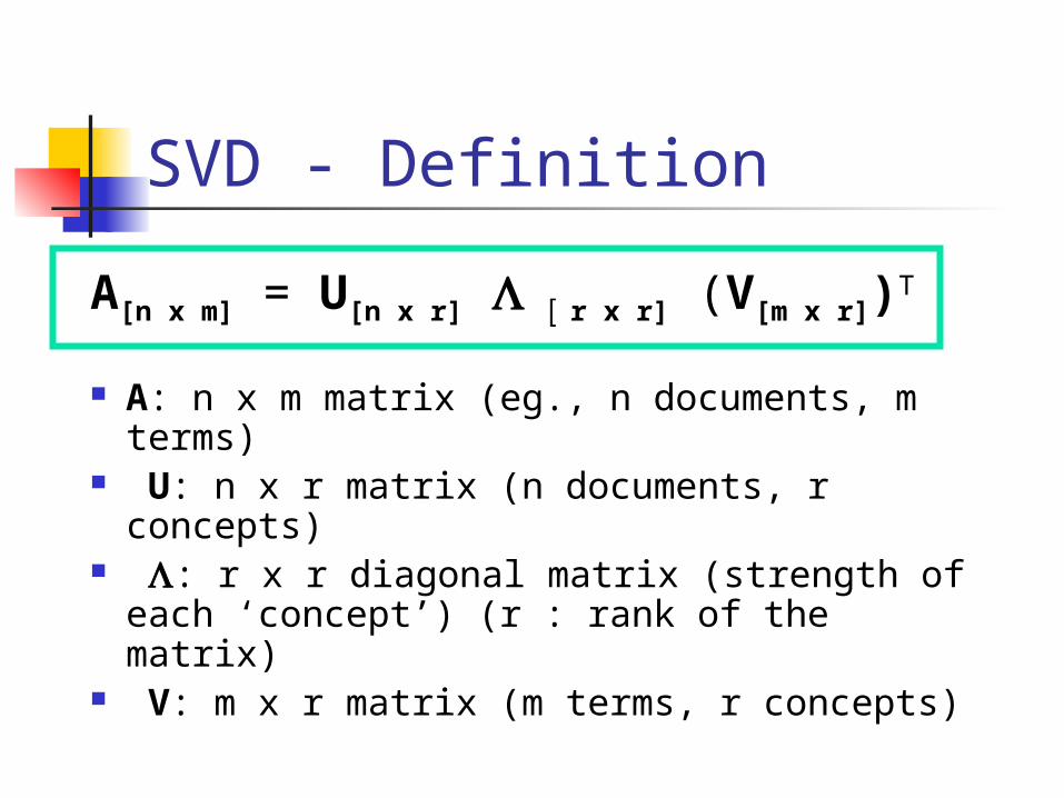
SVD - Definition
A[n x m] = U[n x r] r x r] (V[m x r])T
A: n x m matrix (eg., n documents, m terms)
U: n x r matrix (n documents, r concepts)
: r x r diagonal matrix (strength of each ‘concept’) (r : rank of the matrix)
V: m x r matrix (m terms, r concepts)
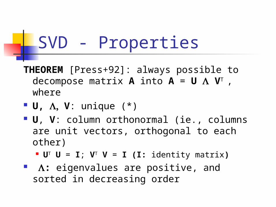
SVD - Properties
THEOREM [Press+92]: always possible to decompose matrix A into A = U VT , where
U, V: unique (*) U, V: column orthonormal (ie., columns
are unit vectors, orthogonal to each other) UT U = I; VT V = I (I: identity matrix)
: eigenvalues are positive, and sorted in decreasing order
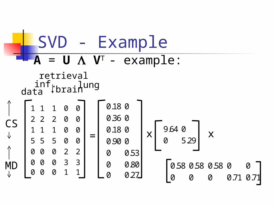
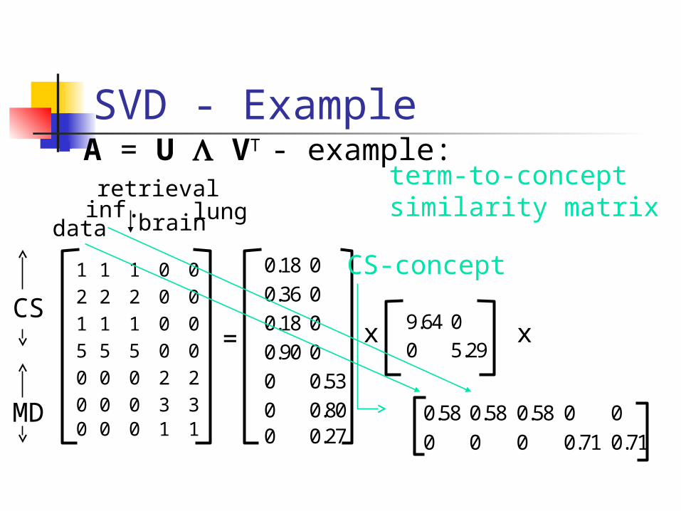
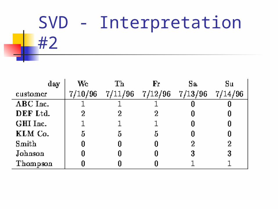
SVD - Example A = U VT - example:
1 1 1 0 0
2 2 2 0 0
1 1 1 0 0
5 5 5 0 0
0 0 0 2 2
0 0 0 3 30 0 0 1 1
datainf.
retrieval
brain lung
0.18 0
0.36 0
0.18 0
0.90 0
0 0.53
0 0.800 0.27
=CS
MD
9.64 0
0 5.29x
0.58 0.58 0.58 0 0
0 0 0 0.71 0.71
x
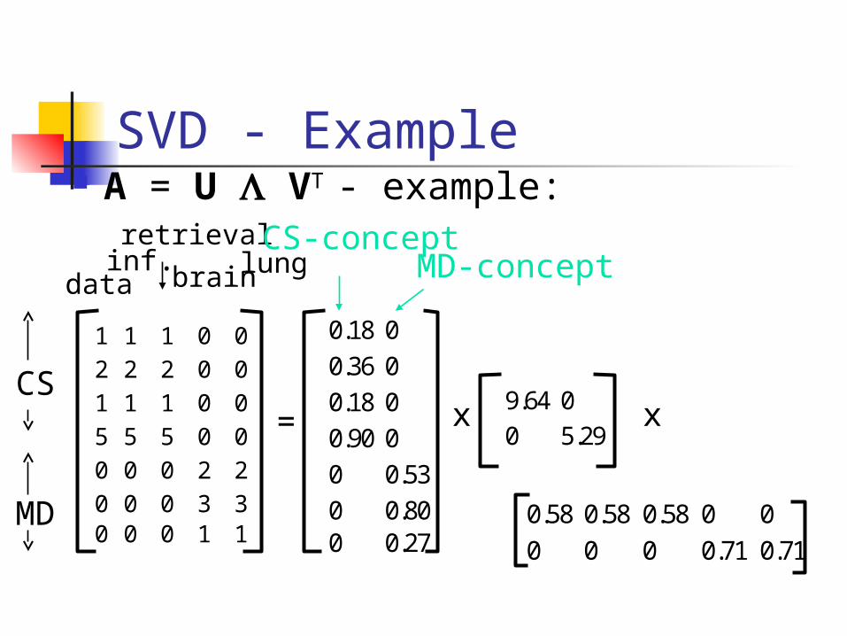
SVD - Example A = U VT - example:
1 1 1 0 0
2 2 2 0 0
1 1 1 0 0
5 5 5 0 0
0 0 0 2 2
0 0 0 3 30 0 0 1 1
datainf.
retrieval
brain lung
0.18 0
0.36 0
0.18 0
0.90 0
0 0.53
0 0.800 0.27
=CS
MD
9.64 0
0 5.29x
0.58 0.58 0.58 0 0
0 0 0 0.71 0.71
x
CS-conceptMD-concept
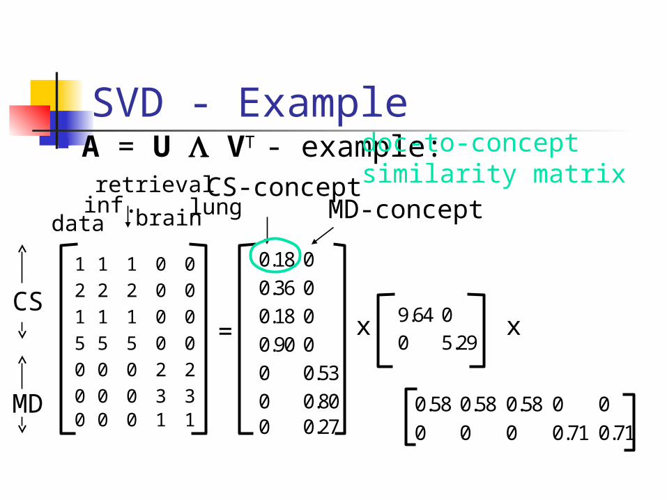
SVD - Example A = U VT - example:
1 1 1 0 0
2 2 2 0 0
1 1 1 0 0
5 5 5 0 0
0 0 0 2 2
0 0 0 3 30 0 0 1 1
datainf.
retrieval
brain lung
0.18 0
0.36 0
0.18 0
0.90 0
0 0.53
0 0.800 0.27
=CS
MD
9.64 0
0 5.29x
0.58 0.58 0.58 0 0
0 0 0 0.71 0.71
x
CS-conceptMD-concept
doc-to-concept similarity matrix
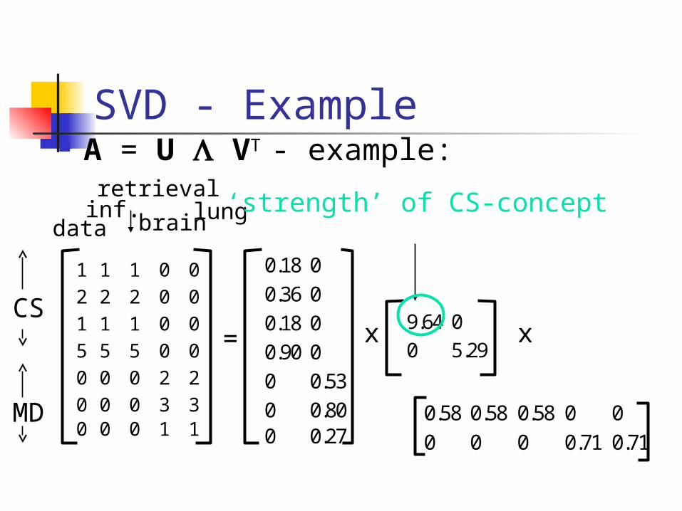
SVD - Example A = U VT - example:
1 1 1 0 0
2 2 2 0 0
1 1 1 0 0
5 5 5 0 0
0 0 0 2 2
0 0 0 3 30 0 0 1 1
datainf.
retrieval
brain lung
0.18 0
0.36 0
0.18 0
0.90 0
0 0.53
0 0.800 0.27
=CS
MD
9.64 0
0 5.29x
0.58 0.58 0.58 0 0
0 0 0 0.71 0.71
x
‘strength’ of CS-concept
SVD - Example A = U VT - example:
1 1 1 0 0
2 2 2 0 0
1 1 1 0 0
5 5 5 0 0
0 0 0 2 2
0 0 0 3 30 0 0 1 1
datainf.
retrieval
brain lung
0.18 0
0.36 0
0.18 0
0.90 0
0 0.53
0 0.800 0.27
=CS
MD
9.64 0
0 5.29x
0.58 0.58 0.58 0 0
0 0 0 0.71 0.71
x
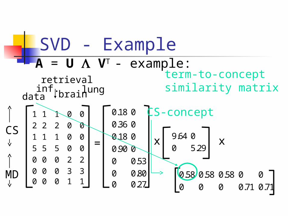
term-to-conceptsimilarity matrix
CS-concept
SVD - Example A = U VT - example:
1 1 1 0 0
2 2 2 0 0
1 1 1 0 0
5 5 5 0 0
0 0 0 2 2
0 0 0 3 30 0 0 1 1
datainf.
retrieval
brain lung
0.18 0
0.36 0
0.18 0
0.90 0
0 0.53
0 0.800 0.27
=CS
MD
9.64 0
0 5.29x
0.58 0.58 0.58 0 0
0 0 0 0.71 0.71
x
term-to-conceptsimilarity matrix
CS-concept
SVD - Detailed outline Motivation Definition - properties Interpretation Complexity Case studies Additional properties
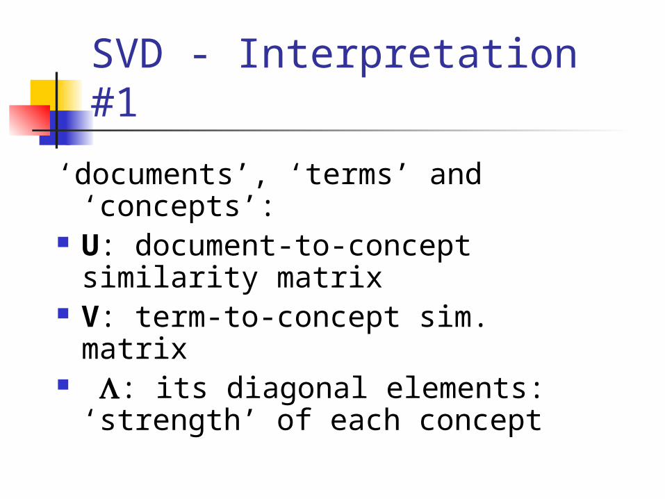
SVD - Interpretation #1
‘documents’, ‘terms’ and ‘concepts’: U: document-to-concept similarity
matrix V: term-to-concept sim. matrix : its diagonal elements:
‘strength’ of each concept
SVD - Interpretation #2 best axis to project on: (‘best’ =
min sum of squares of projection errors)
SVD - Motivation
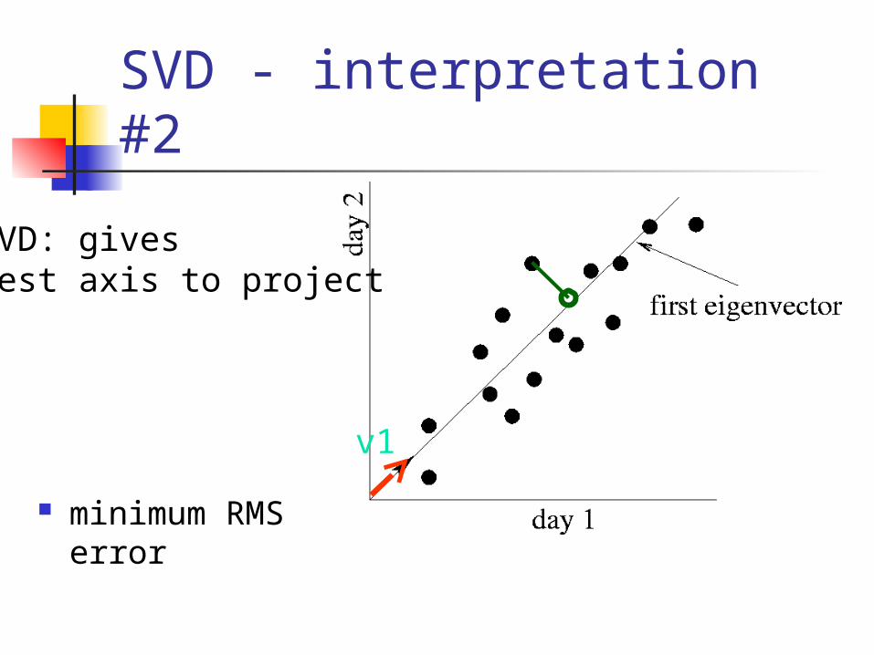
SVD - interpretation #2
minimum RMS error
SVD: givesbest axis to project
v1
SVD - Interpretation #2
SVD - Interpretation #2
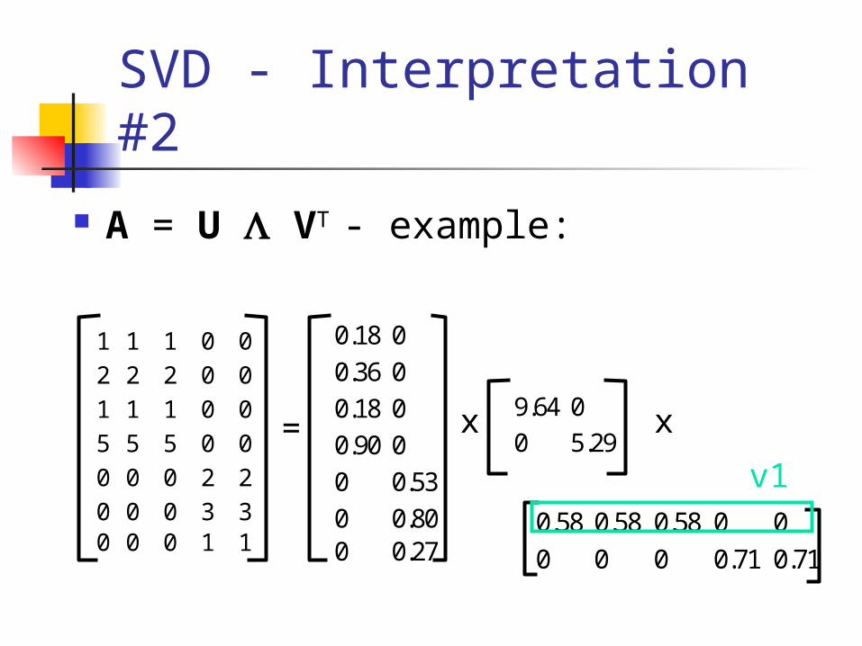
A = U VT - example:
1 1 1 0 0
2 2 2 0 0
1 1 1 0 0
5 5 5 0 0
0 0 0 2 2
0 0 0 3 30 0 0 1 1
0.18 0
0.36 0
0.18 0
0.90 0
0 0.53
0 0.800 0.27
=9.64 0
0 5.29x
0.58 0.58 0.58 0 0
0 0 0 0.71 0.71
x
v1
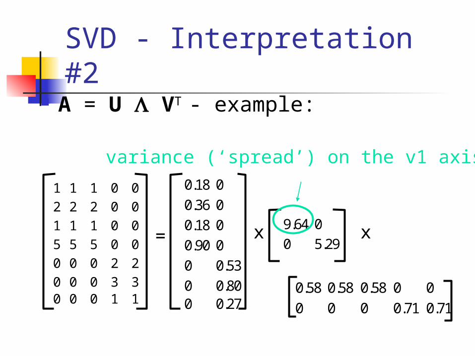
SVD - Interpretation #2 A = U VT - example:
1 1 1 0 0
2 2 2 0 0
1 1 1 0 0
5 5 5 0 0
0 0 0 2 2
0 0 0 3 30 0 0 1 1
0.18 0
0.36 0
0.18 0
0.90 0
0 0.53
0 0.800 0.27
=9.64 0
0 5.29x
0.58 0.58 0.58 0 0
0 0 0 0.71 0.71
x
variance (‘spread’) on the v1 axis
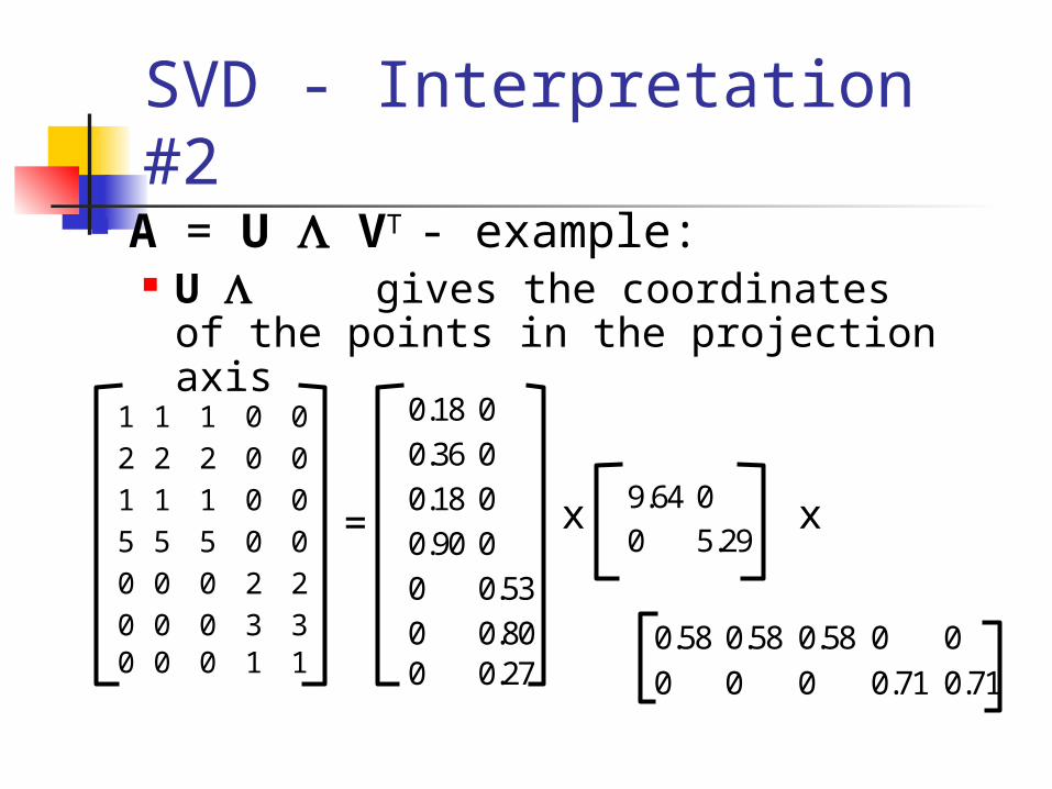
SVD - Interpretation #2 A = U VT - example:
U gives the coordinates of the points in the projection axis
1 1 1 0 0
2 2 2 0 0
1 1 1 0 0
5 5 5 0 0
0 0 0 2 2
0 0 0 3 30 0 0 1 1
0.18 0
0.36 0
0.18 0
0.90 0
0 0.53
0 0.800 0.27
=9.64 0
0 5.29x
0.58 0.58 0.58 0 0
0 0 0 0.71 0.71
x
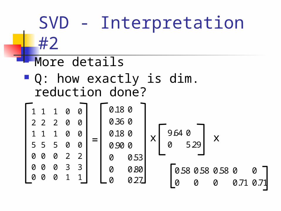
SVD - Interpretation #2 More details Q: how exactly is dim. reduction
done?1 1 1 0 0
2 2 2 0 0
1 1 1 0 0
5 5 5 0 0
0 0 0 2 2
0 0 0 3 30 0 0 1 1
0.18 0
0.36 0
0.18 0
0.90 0
0 0.53
0 0.800 0.27
=9.64 0
0 5.29x
0.58 0.58 0.58 0 0
0 0 0 0.71 0.71
x
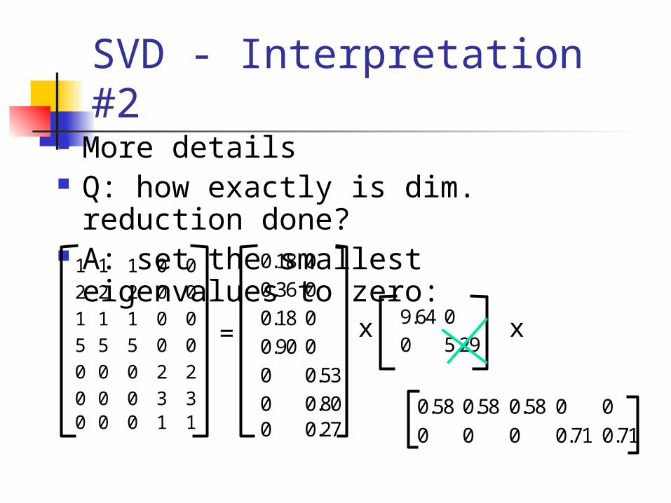
SVD - Interpretation #2 More details Q: how exactly is dim. reduction
done? A: set the smallest eigenvalues to
zero:1 1 1 0 0
2 2 2 0 0
1 1 1 0 0
5 5 5 0 0
0 0 0 2 2
0 0 0 3 30 0 0 1 1
0.18 0
0.36 0
0.18 0
0.90 0
0 0.53
0 0.800 0.27
=9.64 0
0 5.29x
0.58 0.58 0.58 0 0
0 0 0 0.71 0.71
x
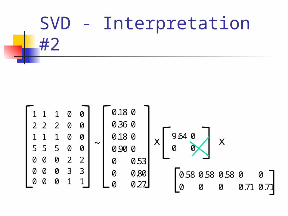
SVD - Interpretation #2
1 1 1 0 0
2 2 2 0 0
1 1 1 0 0
5 5 5 0 0
0 0 0 2 2
0 0 0 3 30 0 0 1 1
0.18 0
0.36 0
0.18 0
0.90 0
0 0.53
0 0.800 0.27
~9.64 0
0 0x
0.58 0.58 0.58 0 0
0 0 0 0.71 0.71
x
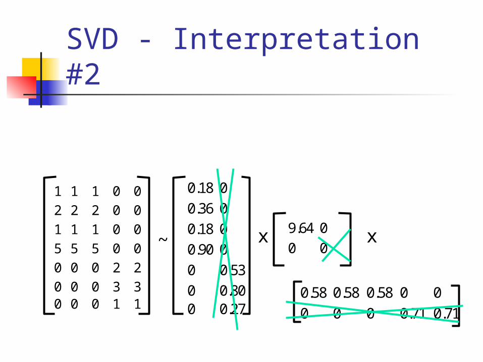
SVD - Interpretation #2
1 1 1 0 0
2 2 2 0 0
1 1 1 0 0
5 5 5 0 0
0 0 0 2 2
0 0 0 3 30 0 0 1 1
0.18 0
0.36 0
0.18 0
0.90 0
0 0.53
0 0.800 0.27
~9.64 0
0 0x
0.58 0.58 0.58 0 0
0 0 0 0.71 0.71
x
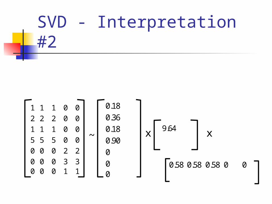
SVD - Interpretation #2
1 1 1 0 0
2 2 2 0 0
1 1 1 0 0
5 5 5 0 0
0 0 0 2 2
0 0 0 3 30 0 0 1 1
0.18
0.36
0.18
0.90
0
00
~9.64
x
0.58 0.58 0.58 0 0
x
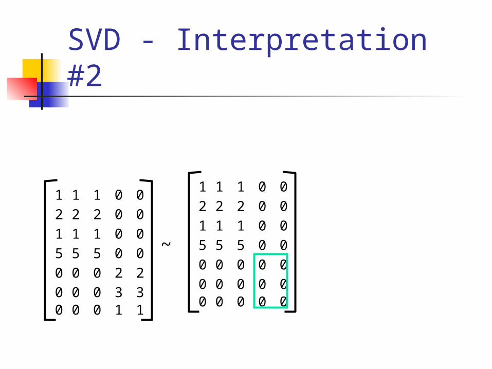
SVD - Interpretation #2
1 1 1 0 0
2 2 2 0 0
1 1 1 0 0
5 5 5 0 0
0 0 0 2 2
0 0 0 3 30 0 0 1 1
~
1 1 1 0 0
2 2 2 0 0
1 1 1 0 0
5 5 5 0 0
0 0 0 0 0
0 0 0 0 00 0 0 0 0
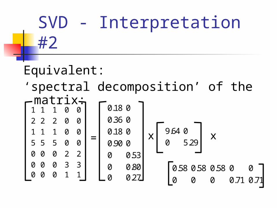
SVD - Interpretation #2
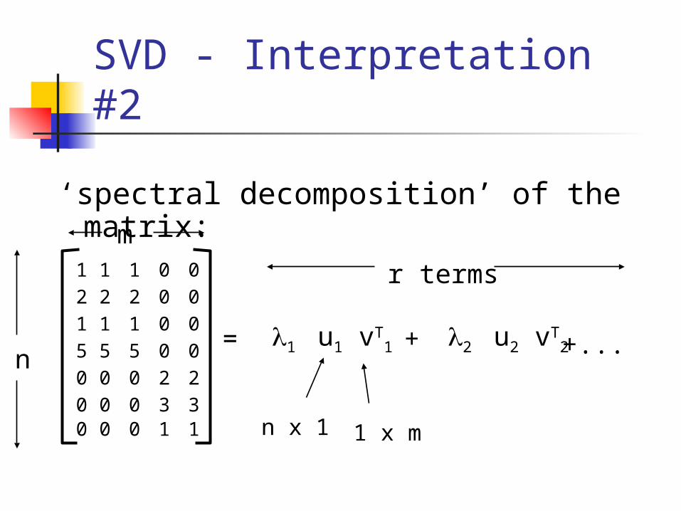
Equivalent:‘spectral decomposition’ of the
matrix:1 1 1 0 0
2 2 2 0 0
1 1 1 0 0
5 5 5 0 0
0 0 0 2 2
0 0 0 3 30 0 0 1 1
0.18 0
0.36 0
0.18 0
0.90 0
0 0.53
0 0.800 0.27
=9.64 0
0 5.29x
0.58 0.58 0.58 0 0
0 0 0 0.71 0.71
x
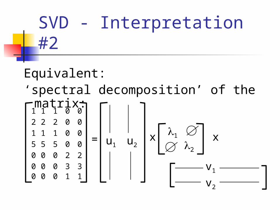
SVD - Interpretation #2
Equivalent:‘spectral decomposition’ of the
matrix:1 1 1 0 0
2 2 2 0 0
1 1 1 0 0
5 5 5 0 0
0 0 0 2 2
0 0 0 3 30 0 0 1 1
= x xu1 u2
1
2
v1
v2
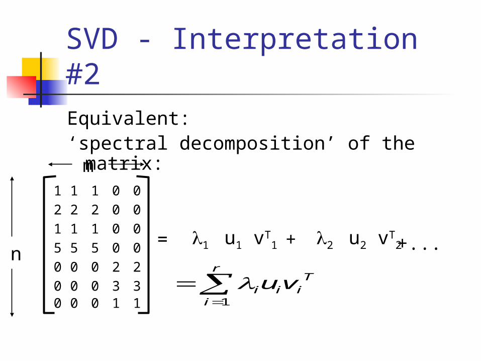
SVD - Interpretation #2Equivalent:‘spectral decomposition’ of the
matrix:1 1 1 0 0
2 2 2 0 0
1 1 1 0 0
5 5 5 0 0
0 0 0 2 2
0 0 0 3 30 0 0 1 1
= u11 vT1 u22 vT
2+ +...n
m
r
i
Tiii vu
1
SVD - Interpretation #2
‘spectral decomposition’ of the matrix:
1 1 1 0 0
2 2 2 0 0
1 1 1 0 0
5 5 5 0 0
0 0 0 2 2
0 0 0 3 30 0 0 1 1
= u11 vT1 u22 vT
2+ +...n
m
n x 1 1 x m
r terms
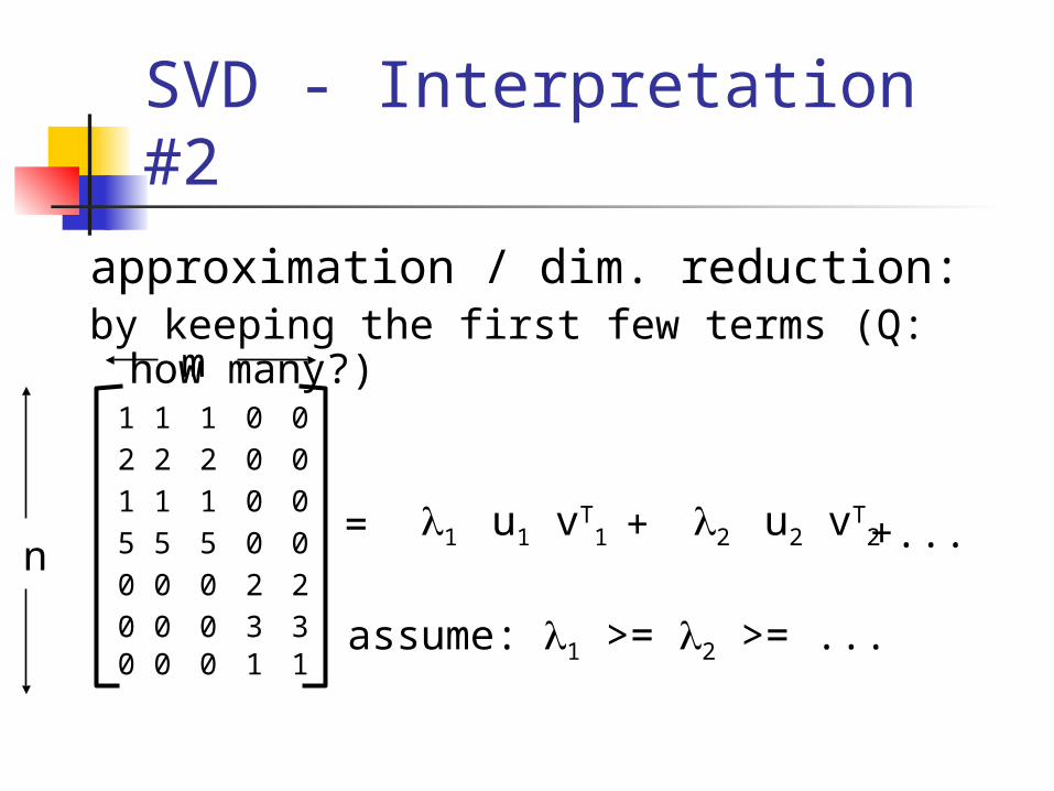
SVD - Interpretation #2
approximation / dim. reduction:by keeping the first few terms (Q: how
many?)1 1 1 0 0
2 2 2 0 0
1 1 1 0 0
5 5 5 0 0
0 0 0 2 2
0 0 0 3 30 0 0 1 1
= u11 vT1 u22 vT
2+ +...n
m
assume: 1 >= 2 >= ...
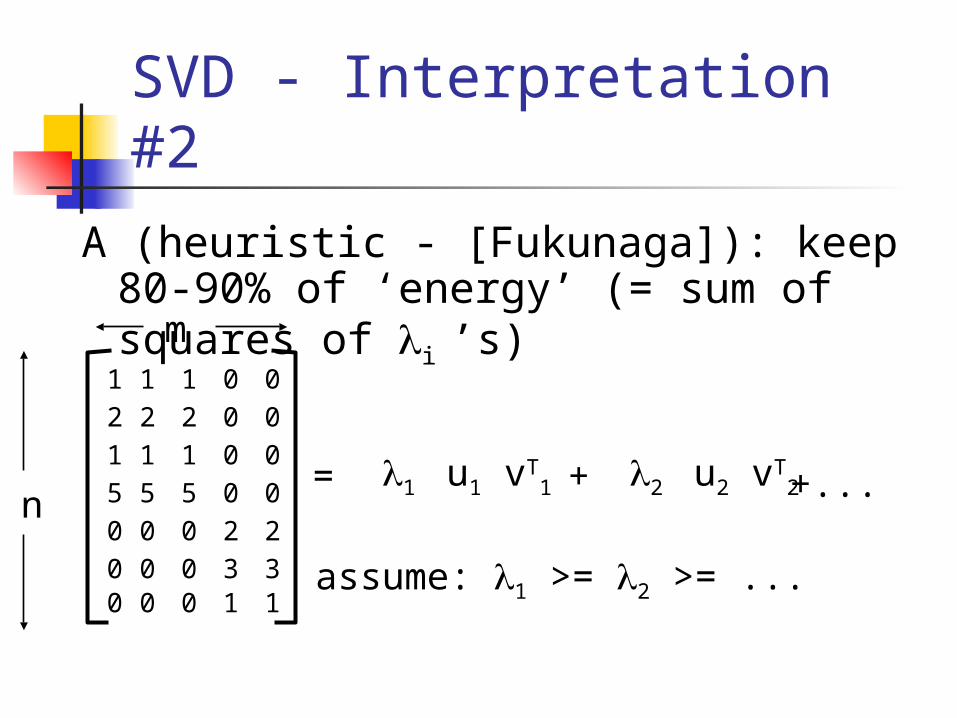
SVD - Interpretation #2
A (heuristic - [Fukunaga]): keep 80-90% of ‘energy’ (= sum of squares of i ’s)
1 1 1 0 0
2 2 2 0 0
1 1 1 0 0
5 5 5 0 0
0 0 0 2 2
0 0 0 3 30 0 0 1 1
= u11 vT1 u22 vT
2+ +...n
m
assume: 1 >= 2 >= ...
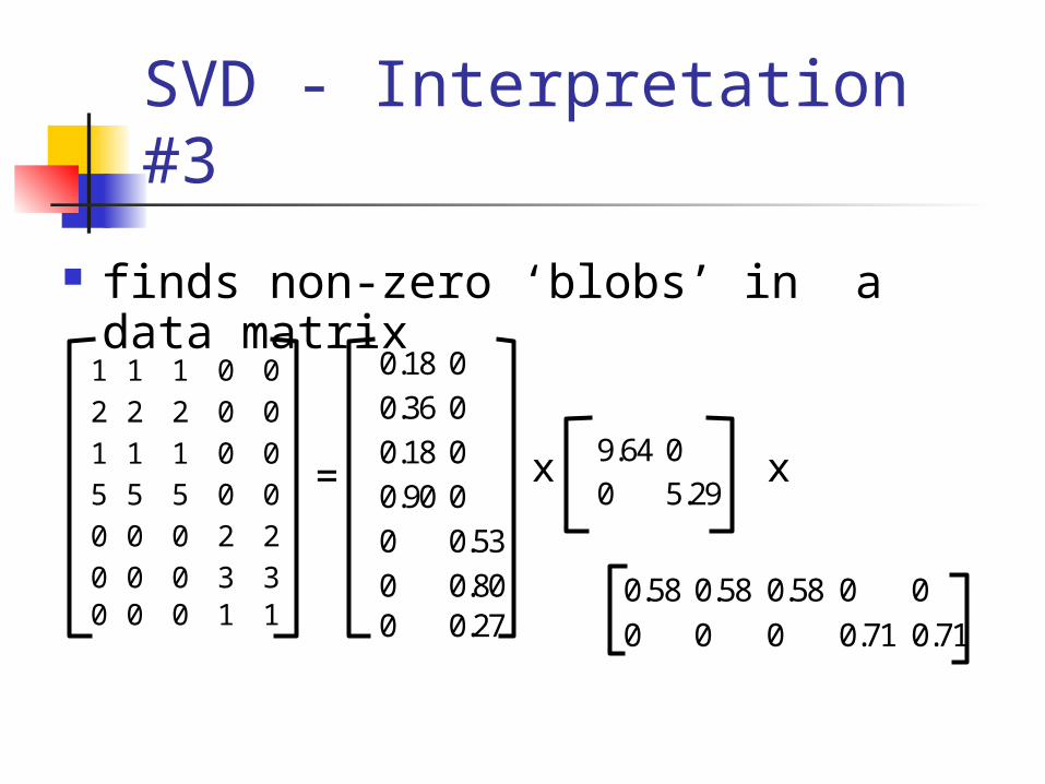
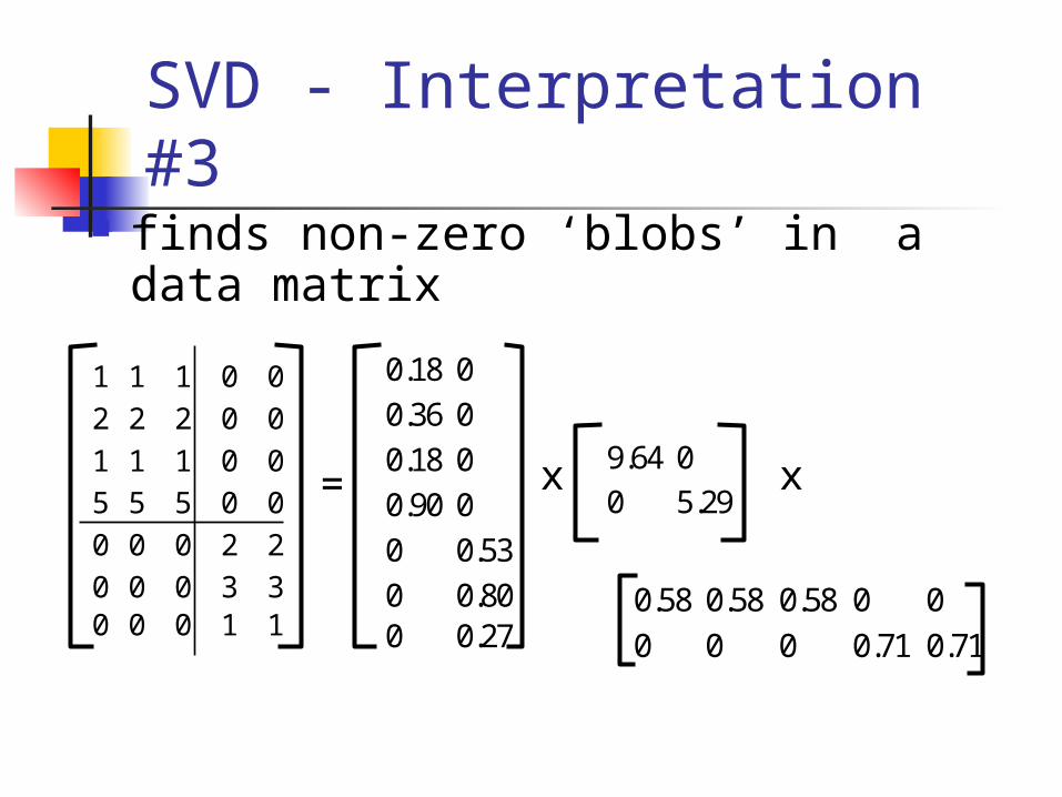
SVD - Interpretation #3
finds non-zero ‘blobs’ in a data matrix
1 1 1 0 0
2 2 2 0 0
1 1 1 0 0
5 5 5 0 0
0 0 0 2 2
0 0 0 3 30 0 0 1 1
0.18 0
0.36 0
0.18 0
0.90 0
0 0.53
0 0.800 0.27
=9.64 0
0 5.29x
0.58 0.58 0.58 0 0
0 0 0 0.71 0.71
x
SVD - Interpretation #3 finds non-zero ‘blobs’ in a data
matrix
1 1 1 0 0
2 2 2 0 0
1 1 1 0 0
5 5 5 0 0
0 0 0 2 2
0 0 0 3 30 0 0 1 1
0.18 0
0.36 0
0.18 0
0.90 0
0 0.53
0 0.800 0.27
=9.64 0
0 5.29x
0.58 0.58 0.58 0 0
0 0 0 0.71 0.71
x
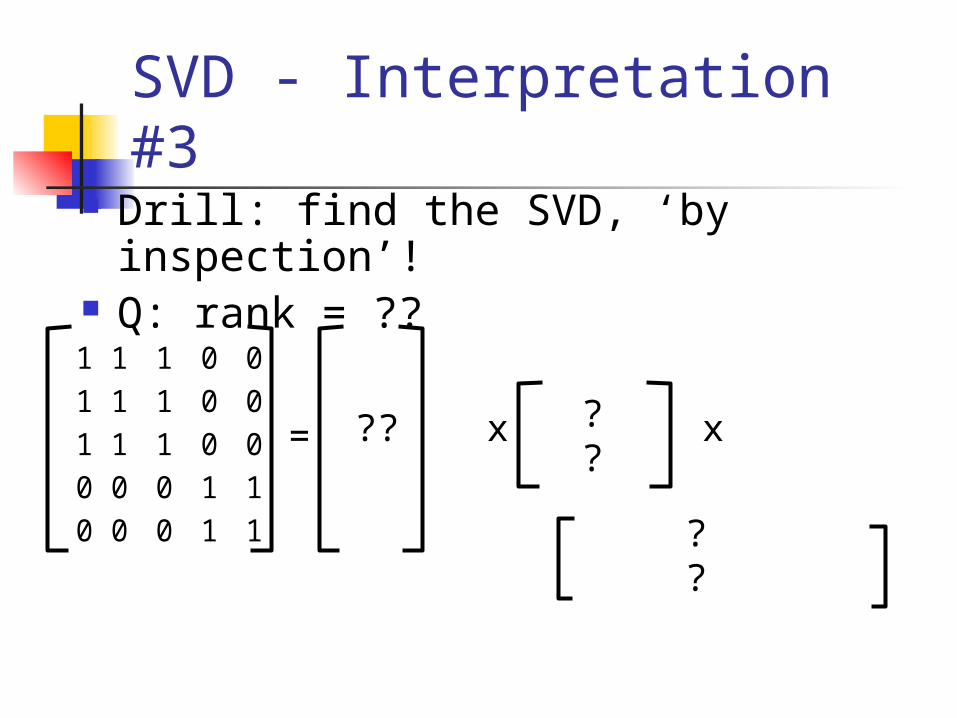
SVD - Interpretation #3 Drill: find the SVD, ‘by inspection’! Q: rank = ??
1 1 1 0 0
1 1 1 0 0
1 1 1 0 0
0 0 0 1 1
0 0 0 1 1
= x x?? ??
??
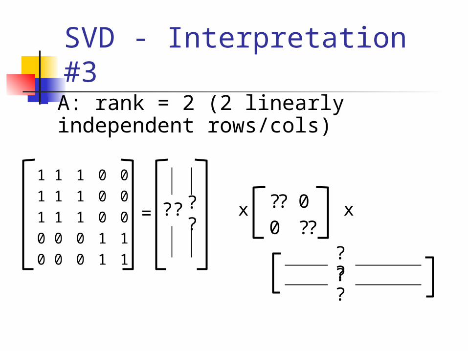
SVD - Interpretation #3 A: rank = 2 (2 linearly independent
rows/cols)
1 1 1 0 0
1 1 1 0 0
1 1 1 0 0
0 0 0 1 1
0 0 0 1 1
= x x??
??
?? 0
0 ??
??
??
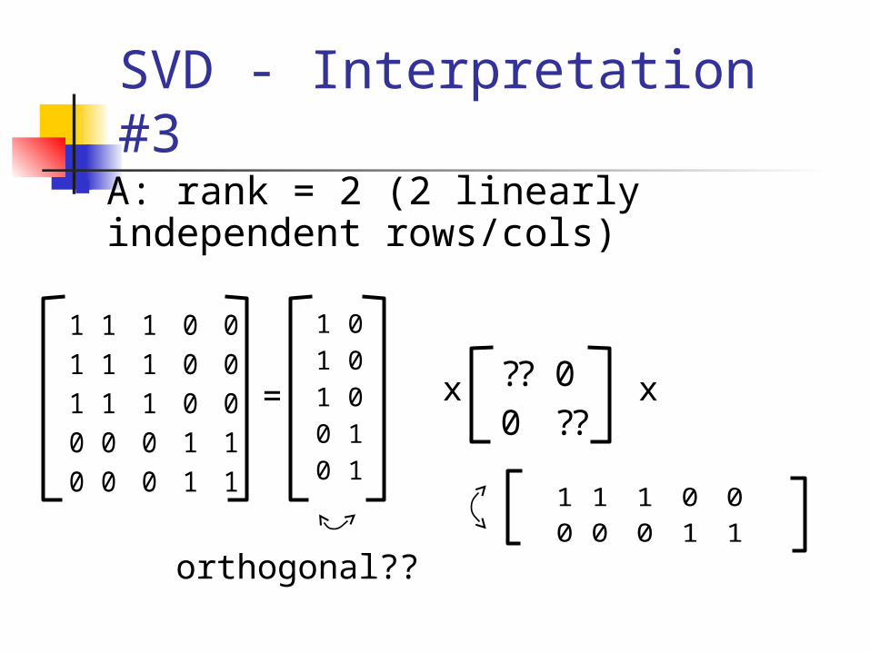
SVD - Interpretation #3 A: rank = 2 (2 linearly independent
rows/cols)
1 1 1 0 0
1 1 1 0 0
1 1 1 0 0
0 0 0 1 1
0 0 0 1 1
= x x?? 0
0 ??
1 0
1 0
1 0
0 1
0 11 1 1 0 0
0 0 0 1 1
orthogonal??
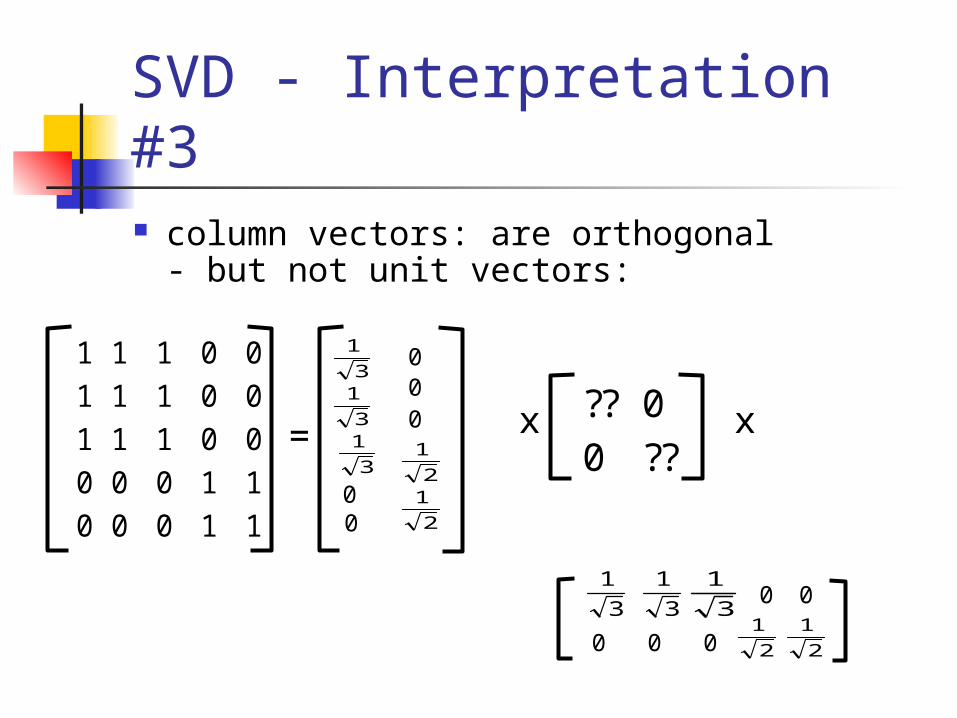
SVD - Interpretation #3 column vectors: are orthogonal -
but not unit vectors:
3
1
1 1 1 0 0
1 1 1 0 0
1 1 1 0 0
0 0 0 1 1
0 0 0 1 1
= x x?? 0
0 ??
3
1
3
1
3
1
3
1
3
1
00
000
2
1
2
1
0 0
0 0 0 2
1
2
1
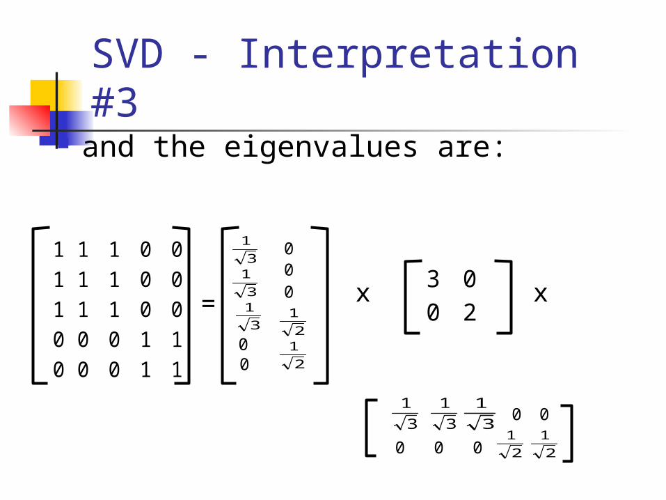
SVD - Interpretation #3 and the eigenvalues are:
1 1 1 0 0
1 1 1 0 0
1 1 1 0 0
0 0 0 1 1
0 0 0 1 1
= x x3 0
0 2
3
1
3
1
3
1
00
000
2
1
2
1
3
1
3
1
3
10 0
0 0 0 2
1
2
1
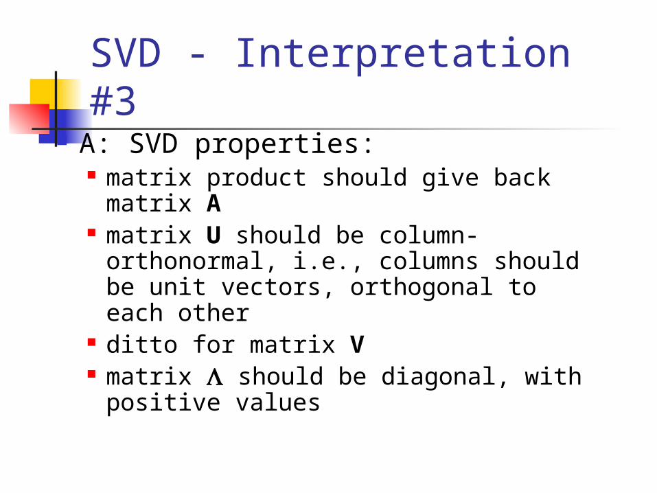
SVD - Interpretation #3 A: SVD properties:
matrix product should give back matrix A
matrix U should be column-orthonormal, i.e., columns should be unit vectors, orthogonal to each other
ditto for matrix V matrix should be diagonal, with
positive values
SVD - Detailed outline Motivation Definition - properties Interpretation Complexity Case studies Additional properties
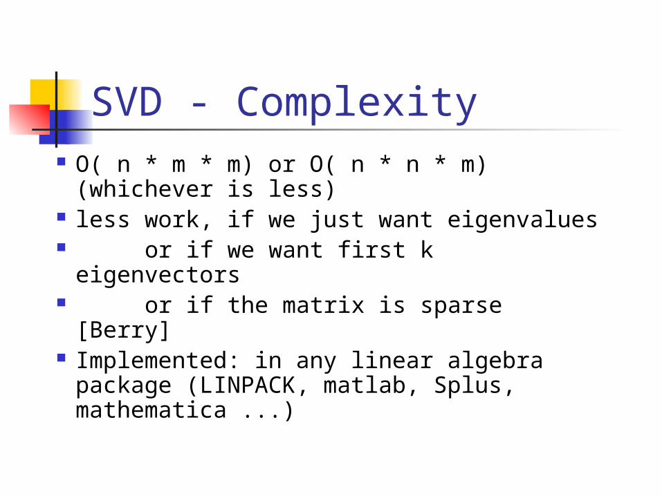
SVD - Complexity O( n * m * m) or O( n * n * m)
(whichever is less) less work, if we just want
eigenvalues or if we want first k eigenvectors or if the matrix is sparse [Berry] Implemented: in any linear algebra
package (LINPACK, matlab, Splus, mathematica ...)
SVD - Complexity Faster algorithms for approximate
eigenvector computations exist: Alan Frieze, Ravi Kannan, Santosh Vempala: Fast Monte-
Carlo Algorithms for finding low-rank approximations, Proceedings of the 39th FOCS, p.370, November 08-11, 1998
Sudipto Guha, Dimitrios Gunopulos, Nick Koudas: Correlating synchronous and asynchronous data streams. KDD 2003: 529-534
SVD - conclusions so far SVD: A= U VT : unique (*) U: document-to-concept similarities V: term-to-concept similarities : strength of each concept dim. reduction: keep the first few
strongest eigenvalues (80-90% of ‘energy’) SVD: picks up linear correlations
SVD: picks up non-zero ‘blobs’
References
Berry, Michael: http://www.cs.utk.edu/~lsi/ Fukunaga, K. (1990). Introduction to Statistical
Pattern Recognition, Academic Press. Press, W. H., S. A. Teukolsky, et al. (1992).
Numerical Recipes in C, Cambridge University Press.


![Spatio-Temporal Data Modelling for 4D -Databases · temporal data [13],[15]. Within the last years a range of temporal models were also developed in the field of object-oriented databases](https://img.pdfslide.net/doc/110x75/5f50ed9e55eedd603937e6c6/spatio-temporal-data-modelling-for-4d-temporal-data-1315-within-the-last.jpg)