The Binomial and Geometric DistributionsChapter 8

8.1 The Binomial Distribution A binomial experiment is statistical experiment

that has the following properties: The experiment consists of n repeated trials. Each trial can result in just two possible outcomes.

We call one of these outcomes a success and the other, a failure.

The probability of success, denoted by P, is the same on every trial.

The trials are independent; that is, the outcome on one trial does not affect the outcome on other trials.

*discrete random variables only

Consider the following statistical experiment. You flip a coin 2 times and count the number of times the coin lands on heads. This is a binomial experiment because: The experiment consists of repeated trials. We flip a coin

2 times. Each trial can result in just two possible outcomes -

heads or tails. The probability of success is constant - 0.5 on every trial. The trials are independent; that is, getting heads on one

trial does not affect whether we get heads on other trials.

Example

Notation x: The number of successes that result from the

binomial experiment. n: The number of trials in the binomial experiment. P: The probability of success on an individual trial. Q: The probability of failure on an individual trial.

(This is equal to 1 - P.) b(x; n, P): Binomial probability - the probability that

an n-trial binomial experiment results in exactly x successes, when the probability of success on an individual trial is P.

Binomial or not? Tossing 20 coins and counting the number of heads.

Yes-1. Success is a heads, failure is a tails. 2. n = 20. 3. Independence is true – coins have no influence on each other. 4. p = .5. So X is B(20, .5). The possible values of X are the integers from 0 to 20.

Picking 5 cards from a standard deck and counting the number of hearts. We replace the card each time and reshuffle. Yes- Success is a heart, failure is anything but a heart. 2. n

= 5. 3. Independence is true. 4. p =.25. So X is B(5, .25). The possible values of X are the integers from 0 to 5.

Picking 5 cards from a standard deck and counting the number of hearts without replacing after each pick. No, b/c of independence issue

Choosing a card from a standard deck until you get a heart. No, b/c there are not a fixed number of observations

It is estimated that 87% of computers users use Explorer as their default web browser. We choose 50 computer users and ask their default browser. Success is Explorer, failure is anything else. 2. n

=50. 3. Independence seems logical. 4. p = .87. So X is B(50, .87). The possible values of X are the integers from 0 to 50.

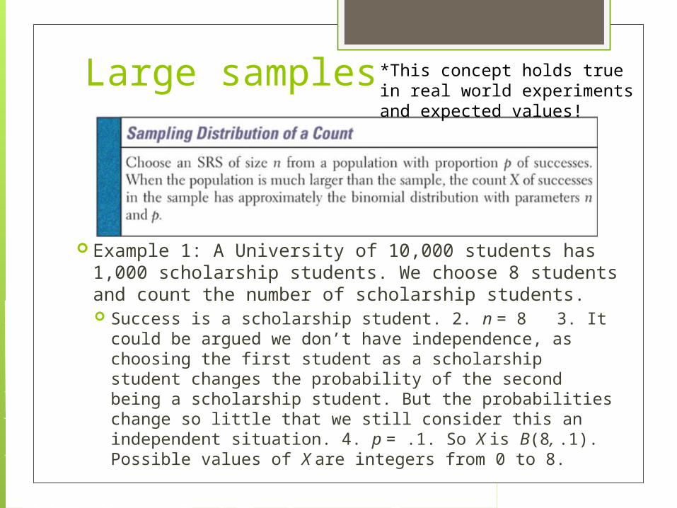
Large samples

Example 1: A University of 10,000 students has 1,000 scholarship students. We choose 8 students and count the number of scholarship students. Success is a scholarship student. 2. n = 8 3. It could

be argued we don’t have independence, as choosing the first student as a scholarship student changes the probability of the second being a scholarship student. But the probabilities change so little that we still consider this an independent situation. 4. p = .1. So X is B(8, .1). Possible values of X are integers from 0 to 8.

*This concept holds true in real world experiments and expected values!

Example 2: An engineer chooses a SRS of 10 switches from a shipment of 10,000 switches. Suppose that (unknown to the engineer) 10% of the switches in the shipment are bad. The engineer counts the number X of bad switches in the sample. This is not quite a binomial setting- just as

removing one card in changes the makeup of the deck, removing one switch changes the proportion of bad switches remaining in the shipment. So the state of the second switch chosen is not independent of the first. BUT removing one switch from a shipment of 10,000 changes the makeup of the remaining 9999 switches very little. In practice, the distribution of X is very close to the binomial distribution with n = 10 and p = .1

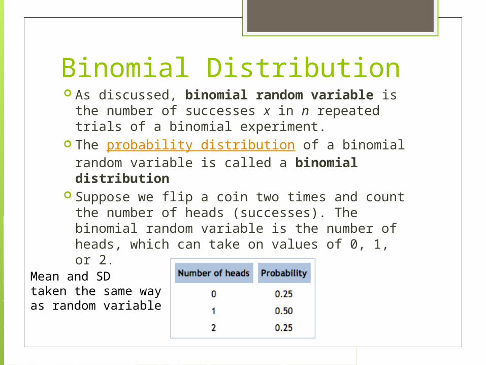
Binomial Distribution As discussed, binomial random variable is

the number of successes x in n repeated trials of a binomial experiment.

The probability distribution of a binomial random variable is called a binomial distribution

Suppose we flip a coin two times and count the number of heads (successes). The binomial random variable is the number of heads, which can take on values of 0, 1, or 2.

Mean and SDtaken the same way as random variable

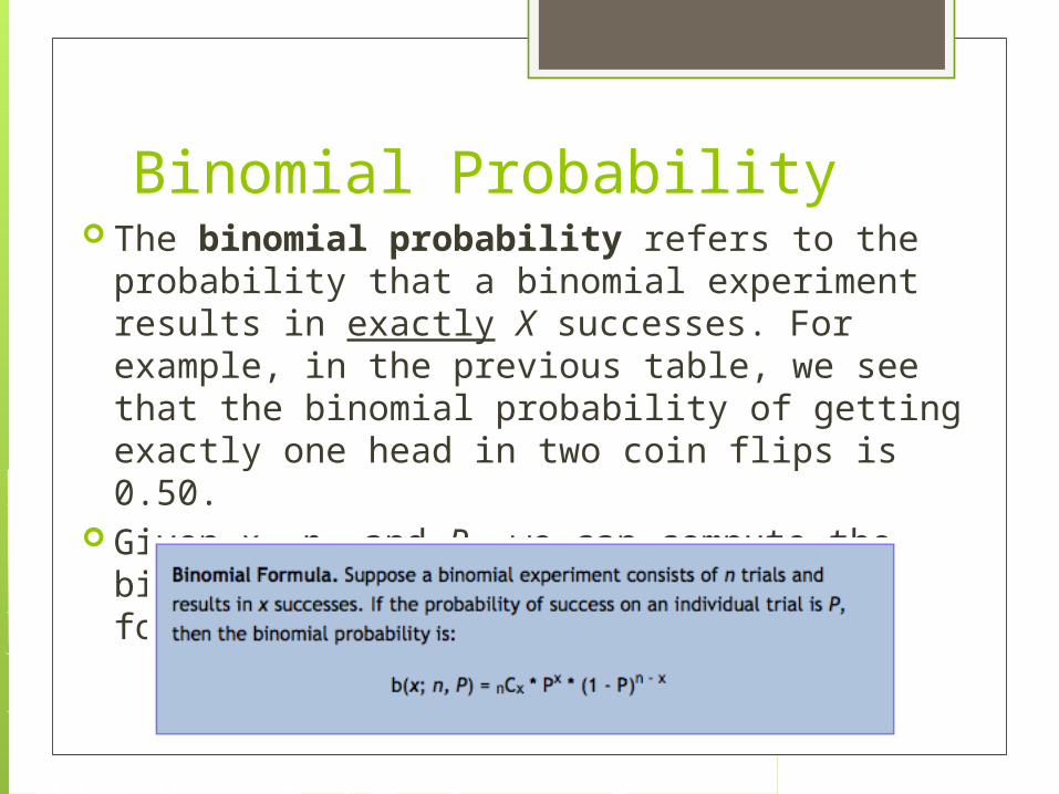
Binomial Probability The binomial probability refers to the

probability that a binomial experiment results in exactly X successes. For example, in the previous table, we see that the binomial probability of getting exactly one head in two coin flips is 0.50.

Given x, n, and P, we can compute the binomial probability based on the following formula (ick!):

Calculator! A Binomial PDF (Probability Density function)

allows you to find the probability that X is any value in a binomial distribution. It is found in the Distribution Menu: 2nd VARS A: binompdf( . Its form is: Binompdf(n, p, X). (There are 3

important variables: n is the number of observations, p is the probability of success, and X is the number of successes you want.

If you don’t specify X, it will give you the probability for all values of X, from 0 to n as a list.

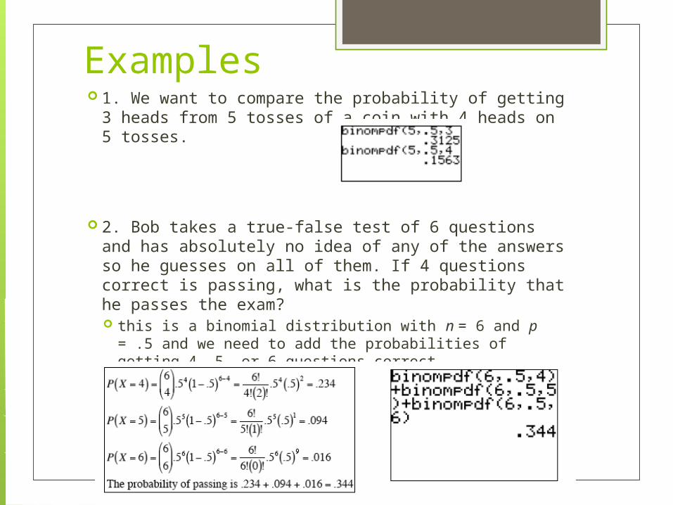
Examples 1. We want to compare the probability of getting 3

heads from 5 tosses of a coin with 4 heads on 5 tosses.

2. Bob takes a true-false test of 6 questions and has absolutely no idea of any of the answers so he guesses on all of them. If 4 questions correct is passing, what is the probability that he passes the exam? this is a binomial distribution with n = 6 and p = .5 and

we need to add the probabilities of getting 4, 5, or 6 questions correct.

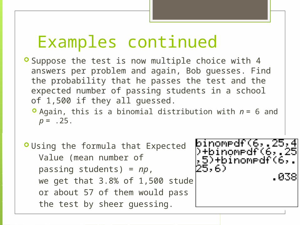
Examples continued Suppose the test is now multiple choice with 4 answers

per problem and again, Bob guesses. Find the probability that he passes the test and the expected number of passing students in a school of 1,500 if they all guessed. Again, this is a binomial distribution with n = 6 and p = .25.

Using the formula that Expected Value (mean number of passing students) = np, we get that 3.8% of 1,500 students or about 57 of them would pass the test by sheer guessing.

Cumulative Binomial Probability A cumulative binomial probability refers to the

probability that the binomial random variable falls within a specified range (e.g., is greater than or equal to a stated lower limit and less than or equal to a stated upper limit).

Ex: In a particular city, 63% of the adults own their home and 37% rent. A sample of 20 adults is taken. Find the probability that the sample will have at least half home-owners. This is binomial with n = 20 and p = .63. We want the value

of X = 10, 11, 12, 13, 14, 15, 16, 17, 18, 19, 20. That is a lot of work, even with the Binompdf function!

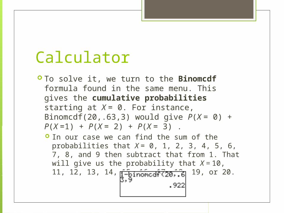
Calculator To solve it, we turn to the Binomcdf formula

found in the same menu. This gives the cumulative probabilities starting at X = 0. For instance, Binomcdf(20,.63,3) would give P(X = 0) + P(X =1) + P(X = 2) + P(X = 3) . In our case we can find the sum of the

probabilities that X = 0, 1, 2, 3, 4, 5, 6, 7, 8, and 9 then subtract that from 1. That will give us the probability that X = 10, 11, 12, 13, 14, 15, 16, 17, 18, 19, or 20.

More Examples 1. What is the probability of obtaining 45 or fewer

heads in 100 tosses of a coin? The sum of all these probabilities is the answer we seek:

b(x = 0; 100, 0.5) + b(x = 1; 100, 0.5) + . . . + b(x = 45; 100, 0.5)

b(x < 45; 100, 0.5) = 0.184 *try on calc!

2. The probability that a student is accepted to a prestigious college is 0.3. If 5 students from the same school apply, what is the probability that at most 2 are accepted? b(x < 2; 5, 0.3) = 0.8369 on calc: binomcdf(5, .3, 2)

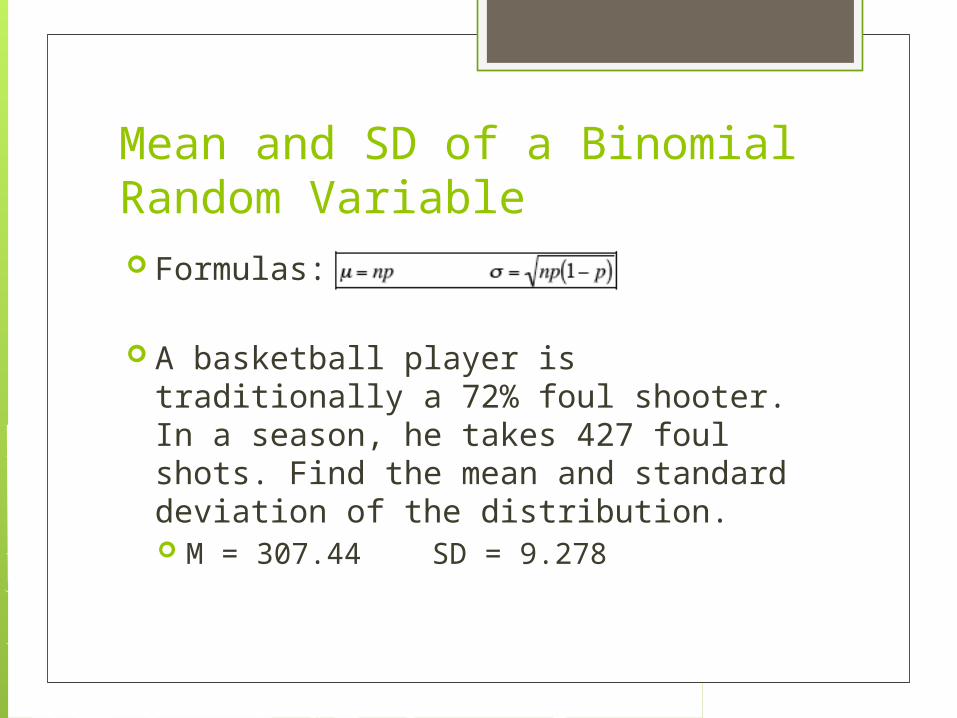
Mean and SD of a Binomial Random Variable Formulas:

A basketball player is traditionally a 72% foul shooter. In a season, he takes 427 foul shots. Find the mean and standard deviation of the distribution. M = 307.44 SD = 9.278

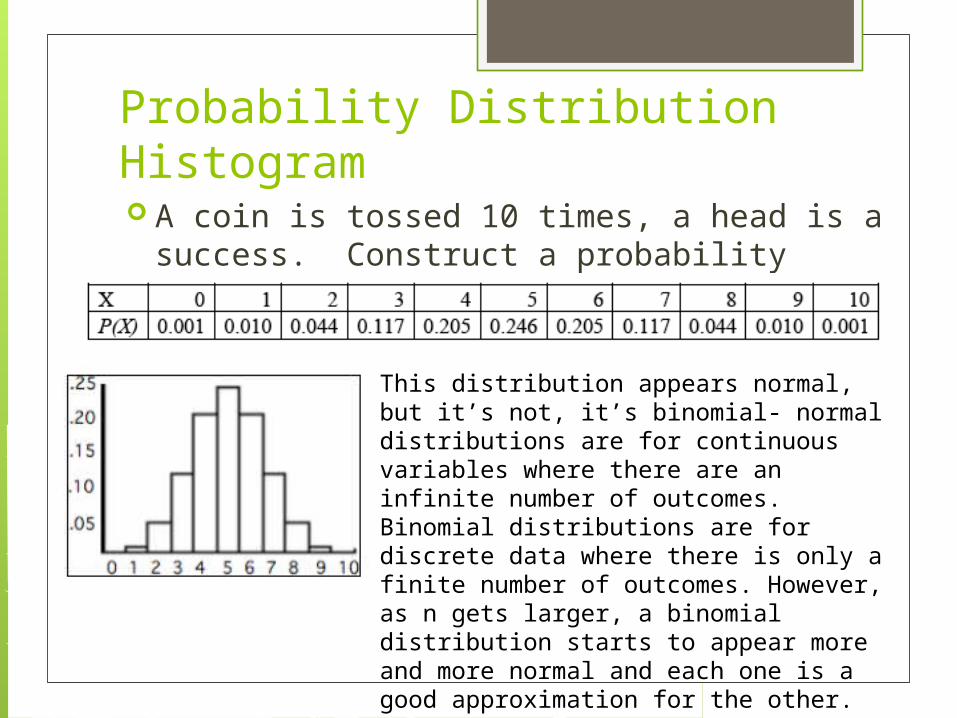
Probability Distribution Histogram A coin is tossed 10 times, a head is a success.

Construct a probability distribution histogram

This distribution appears normal, but it’s not, it’s binomial- normal distributions are for continuous variables where there are an infinite number of outcomes. Binomial distributions are for discrete data where there is only a finite number of outcomes. However, as n gets larger, a binomial distribution starts to appear more and more normal and each one is a good approximation for the other.

Binomial distribution histograms To do this on your calculator:

Enter the values of X in L1 Enter the binomial probabilities into list L2:

Highlight L2 and press 2nd VARS(DISTR) – binompdf(n, p, L1) and hit enter. L2 should populate

Define Plot1 to be a histogram with Xlist: L1 and Freq: L2

Set your X and Y viewing window to cover all your values of X and the probabilities: X(0,10,1) Y(0,.4,.1)

Histograms cont. To do a cumulative histogram on your

calc, make L3 your cumulative probabilities by highlighting L3 and defining it as binomcdf(n, p, L1) ENTER and it will populate.

Make a histogram with Xlist: L1 and Ylist: L3 and adjust viewing window.

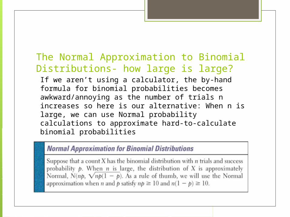
The Normal Approximation to Binomial Distributions- how large is large?If we aren’t using a calculator, the by-hand formula for binomial probabilities becomes awkward/annoying as the number of trials n increases so here is our alternative: When n is large, we can use Normal probability calculations to approximate hard-to-calculate binomial probabilities

Example: Are attitudes toward shopping changing?

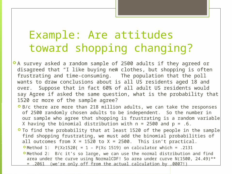
A survey asked a random sample of 2500 adults if they agreed or disagreed that “I like buying new clothes, but shopping is often frustrating and time-consuming.” The population that the poll wants to draw conclusions about is all US residents aged 18 and over. Suppose that in fact 60% of all adult US residents would say Agree if asked the same question, what is the probability that 1520 or more of the sample agree? B/c there are more than 218 million adults, we can take the responses of

2500 randomly chosen adults to be independent. So the number in our sample who agree that shopping is frustrating is a random variable X having the binomial distribution with n = 2500 and p = .6.

To find the probability that at least 1520 of the people in the sample find shopping frustrating, we must add the binomial probabilities of all outcomes from X = 1520 to X = 2500. This isn’t practical. Method 1: P(X≥1520( = 1 – P(X≤ 1519) on calculator which = .2131 Method 2: B/c it’s so large, we can use the normal distribution and find area

under the curve using NormalCDF! So area under curve N(1500, 24.49)** = .2061 (we’re only off from the actual calculation by .0007!)

Geometric Distributions The geometric distribution is a special case

of the binomial distribution. It deals with the number of trials required to obtain your first success.

An example of a geometric distribution would be tossing a coin until it lands on heads. We might ask: What is the probability that the first head occurs on the third flip? That probability is referred to as a geometric probability and is denoted by g(x; P).

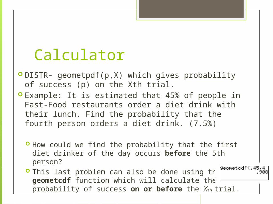
Calculator DISTR- geometpdf(p,X) which gives probability of

success (p) on the Xth trial. Example: It is estimated that 45% of people in

Fast-Food restaurants order a diet drink with their lunch. Find the probability that the fourth person orders a diet drink. (7.5%)

How could we find the probability that the first diet drinker of the day occurs before the 5th person?

This last problem can also be done using the geometcdf function which will calculate the probability of success on or before the Xth trial.

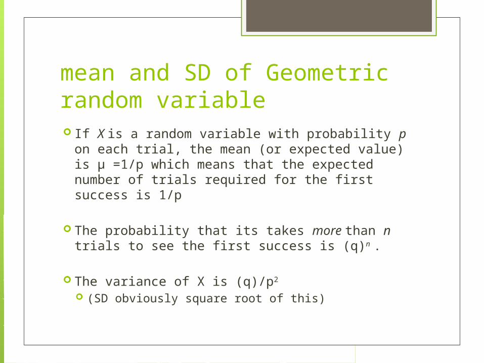
mean and SD of Geometric random variable If X is a random variable with probability p on

each trial, the mean (or expected value) is μ =1/p which means that the expected number of trials required for the first success is 1/p

The probability that its takes more than n trials to see the first success is (q)n .

The variance of X is (q)/p2 (SD obviously square root of this)

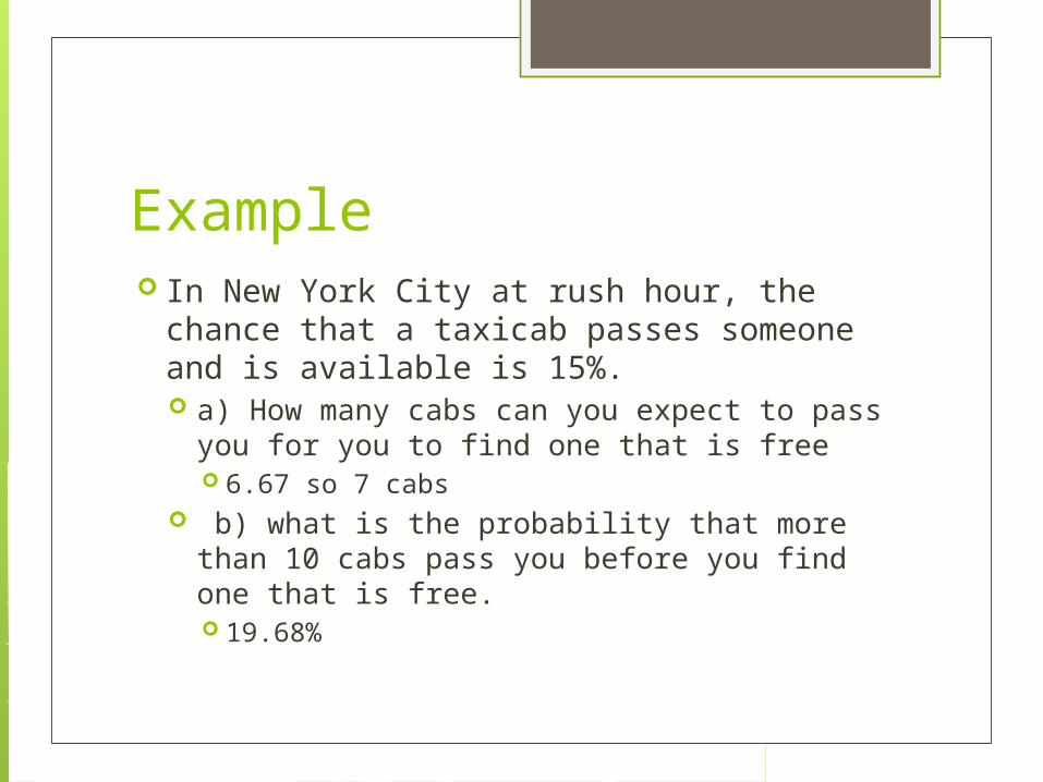
Example In New York City at rush hour, the chance

that a taxicab passes someone and is available is 15%. a) How many cabs can you expect to pass

you for you to find one that is free 6.67 so 7 cabs

b) what is the probability that more than 10 cabs pass you before you find one that is free. 19.68%

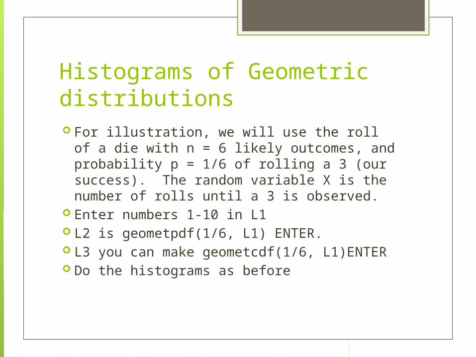
Histograms of Geometric distributions For illustration, we will use the roll of a die

with n = 6 likely outcomes, and probability p = 1/6 of rolling a 3 (our success). The random variable X is the number of rolls until a 3 is observed.

Enter numbers 1-10 in L1 L2 is geometpdf(1/6, L1) ENTER. L3 you can make geometcdf(1/6, L1)ENTER Do the histograms as before