The Concave-Convex Procedure (CCCP)

The Concave-Convex Procedure (CCCP).

Alan YuilleDepartment of Statistics

University of California at Los AngelesLos Angeles, CA 90095

[email protected]

Anand RangarajanDepartment of Computer Science

University of Florida

In Neural Computation. Vol. 15. No. 4. pp 915-936. April. 2003.

1

The Concave-Convex Procedure (CCCP)

A. L. Yuille and Anand Rangarajan ∗

Smith-Kettlewell Eye Research Institute,

2318 Fillmore Street,

San Francisco, CA 94115, USA.

Tel. (415) 345-2144. Fax. (415) 345-8455.

Email [email protected]

December 23, 2002

∗ Prof. Anand Rangarajan. Dept. of CISE, Univ. of Florida Room 301, CSE

Building Gainesville, FL 32611-6120 Phone: (352) 392 1507 Fax: (352) 392 1220

e-mail: [email protected]

Submitted to Neural Computation on 17 April 2002.

Revised 21 July 2002.

Final Revision 27 August 2002.

Abstract

The Concave-Convex procedure (CCCP) is a way to construct discrete time it-

erative dynamical systems which are guaranteed to monotonically decrease global

optimization/energy functions. This procedure can be applied to almost any op-

timization problem and many existing algorithms can be interpreted in terms of

1

Draft submitted to Neural Computation

it. In particular, we prove that all EM algorithms and classes of Legendre min-

imization and variational bounding algorithms can be re-expressed in terms of

CCCP. We show that many existing neural network and mean field theory al-

gorithms are also examples of CCCP. The Generalized Iterative Scaling (GIS)

algorithm and Sinkhorn’s algorithm can also be expressed as CCCP by changing

variables. CCCP can be used both as a new way to understand, and prove con-

vergence of, existing optimization algorithms and as a procedure for generating

new algorithms.

1 Introduction

This paper describes a simple geometrical Concave-Convex procedure (CCCP) for

constructing discrete time dynamical systems which are guaranteed to decrease

almost any global optimization/energy function monotonically. Such discrete time

systems have advantages over standard gradient descent techniques (Press, Flan-

nery, Teukolsky and Vetterling 1986) because they do not require estimating a

step size and empirically often converge rapidly.

We first illustrate CCCP by giving examples of neural network, mean field, and

self-annealing (which relate to Bregman distances (Bregman 1967)) algorithms

which can be re-expressed in this form. As we will show, the entropy terms

arising in mean field algorithms makes it particularly easy to apply CCCP. CCCP

has also been applied to develop an algorithm which minimizes the Bethe and

Kikuchi free energies and whose empirical convergence is rapid (Yuille 2002).

Next we prove that many existing algorithms can be directly re-expressed in

terms of CCCP. This includes expectation-maximization (EM) algorithms (Demp-

2


ster, Laird and Rubin 1977), minimization algorithms based on Legendre trans-

forms (Rangarajan, Yuille and Mjolsness 1999). CCCP can be viewed as a spe-

cial case of variational bounding (Rustagi 1976, Jordan, Ghahramani, Jaakkola

and Saul 1999) and related techniques including lower bound maximization/upper

bound minimization (Luttrell 1994), surrogate functions and majorization (Lange,

Hunter and Yang 2000). CCCP gives a novel geometric perspective on these al-

gorithms and yields new convergence proofs.

Finally we reformulate other classic algorithms in terms of CCCP by changing

variables. These include the Generalized Iterative Scaling (GIS) algorithm (Dar-

roch and Ratcliff 1972) and Sinkhorn’s algorithm for obtaining doubly stochastic

matrices (Sinkhorn 1964). Sinkhorn’s algorithm can be used to solve the linear

assignment problem (Kosowsky and Yuille 1994) and CCCP variants of Sinkhorn

can be used to solve additional constraint problems.

We introduce CCCP in section (2) and prove that it converges. Section (3)

illustrates CCCP with examples from neural networks, mean field theory, self-

annealing, and EM. In section (4.2) we prove the relationships between CCCP and

the EM algorithm, Legendre transforms, and variational bounding. Section (5)

shows that other algorithms such as GIS and Sinkhorn can be expressed in CCCP

by a change of variables.

2 The Concave-Convex Procedure (CCCP)

This section introduces the main results of CCCP and summarizes them in three

Theorems: (i) Theorem 1 states the general conditions under which CCCP can be

applied, (ii) Theorem 2 defines CCCP and proves its convergence, and (iii) Theo-

3


rem 3 describes an inner loop that may be necessary for some CCCP algorithms.

Theorem 1 shows that any function, subject to weak conditions, can be ex-

pressed as the sum of a convex and concave part (this decomposition is not

unique). This will imply that CCCP can be applied to almost any optimization

problem.

Theorem 1. Let E(~x) be an energy function with bounded Hessian ∂2E(~x)/∂~x∂~x.

Then we can always decompose it into the sum of a convex function and a concave

function.

Proof. Select any convex function F (~x) with positive definite Hessian with

eigenvalues bounded below by ε > 0. Then there exists a positive constant λ such

that the Hessian of E(~x) + λF (~x) is positive definite and hence E(~x) + λF (~x) is

convex. Hence we can express E(~x) as the sum of a convex part, E(~x) + λF (~x),

and a concave part −λF (~x).

Theorem 2 defines the CCCP procedure and proves that it converges to a

minimum or a saddle point of the energy function. (After completing this work

we found that a version of Theorem 2 appeared in an unpublished technical report

by D. Geman (1984)).

Theorem 2. Consider an energy function E(~x) (bounded below) of form

E(~x) = Evex(~x) + Ecave(~x) where Evex(~x), Ecave(~x) are convex and concave func-

tions of ~x respectively. Then the discrete iterative CCCP algorithm ~xt 7→ ~xt+1

given by:

~∇Evex(~xt+1) = −~∇Ecave(~x

t), (1)

is guaranteed to monotonically decrease the energy E(~x) as a function of time and

hence to converge to a minimum or saddle point of E(~x) (or even a local maxima

4


−10 −5 0 5 10−1

0

1

2

3

4

5

6

−10 −5 0 5 10−20

0

20

40

60

80

100

120

−10 −5 0 5 10−100

−80

−60

−40

−20

0

20

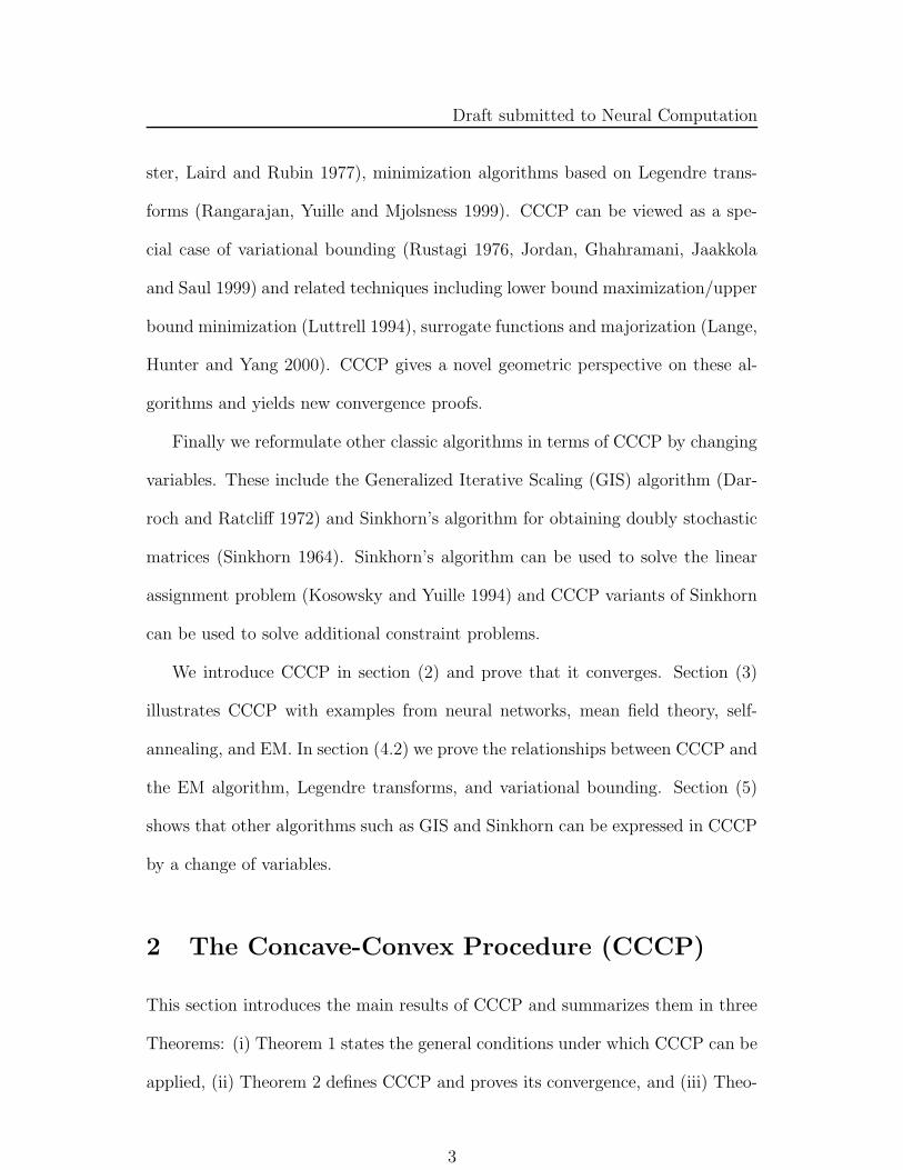
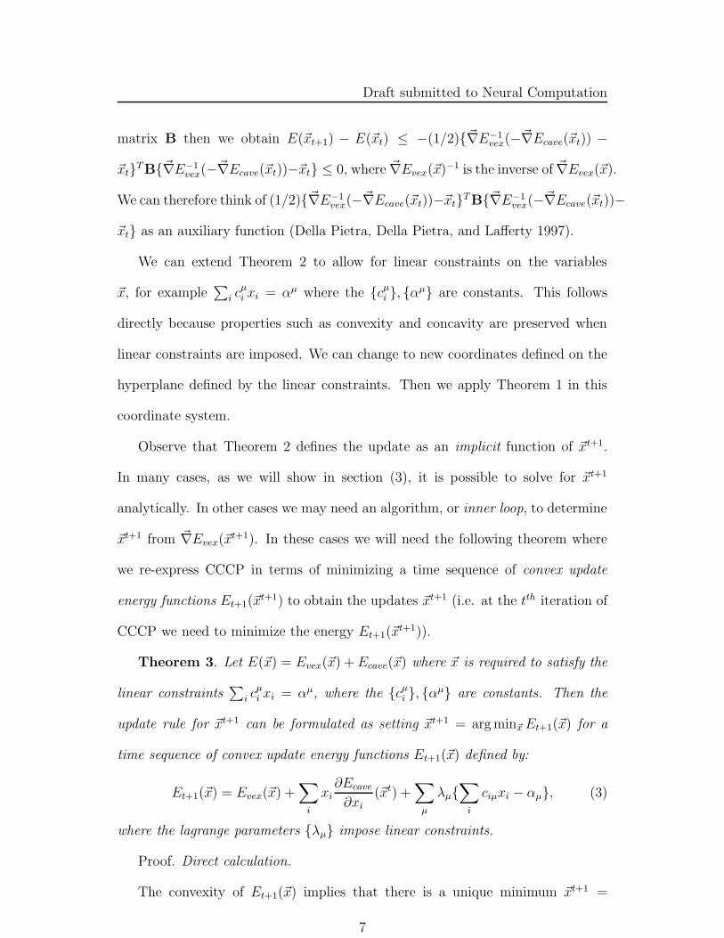
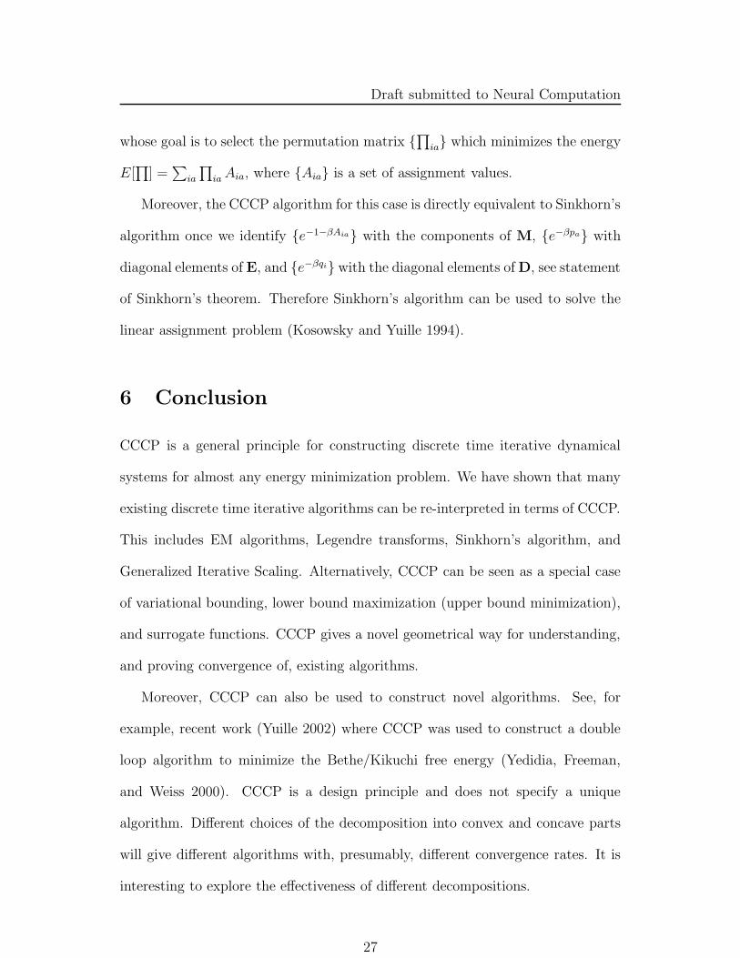
Figure 1: Decomposing a function into convex and concave parts. The original

function (Top Panel) can be expressed as the sum of a convex function (Bottom

Left Panel) and a concave function (Bottom Right Panel).

if it starts at one). Moreover,

E(~xt+1) = E(~xt)−1

2(~xt+1 − ~xt)

T{~∇~∇Evex(~x∗)− ~∇~∇Ecave(~x

∗∗)}(~xt+1 − ~xt), (2)

for some ~x∗ and ~x∗∗, where ~∇~∇E(.) is the Hessian of E(.).

Proof. The convexity and concavity of Evex(.) and Ecave(.) means that Evex(~x2) ≥

Evex(~x1)+(~x2−~x1) · ~∇Evex(~x1) and Ecave(~x4) ≤ Ecave(~x3)+(~x4−~x3) · ~∇Ecave(~x3),

for all ~x1, ~x2, ~x3, ~x4. Now set ~x1 = ~xt+1, ~x2 = ~xt, ~x3 = ~xt, ~x4 = ~xt+1. Using the

algorithm definition (i.e. ~∇Evex(~xt+1) = −~∇Ecave(~x

t)) we find that Evex(~xt+1) +

Ecave(~xt+1) ≤ Evex(~x

t)+Ecave(~xt), which proves the first claim. The second claim

follows by computing the second order terms of the Taylor series expansion and

5


applying Rolle’s theorem.

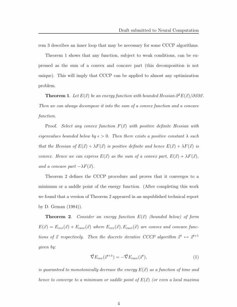
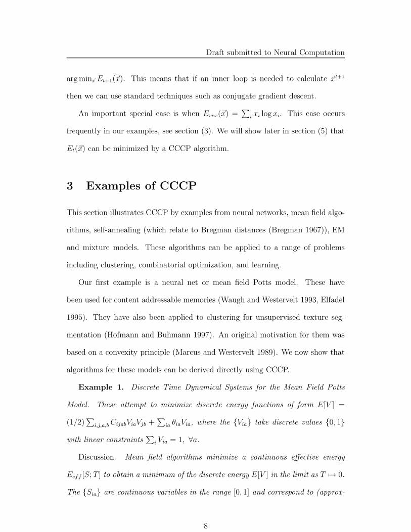
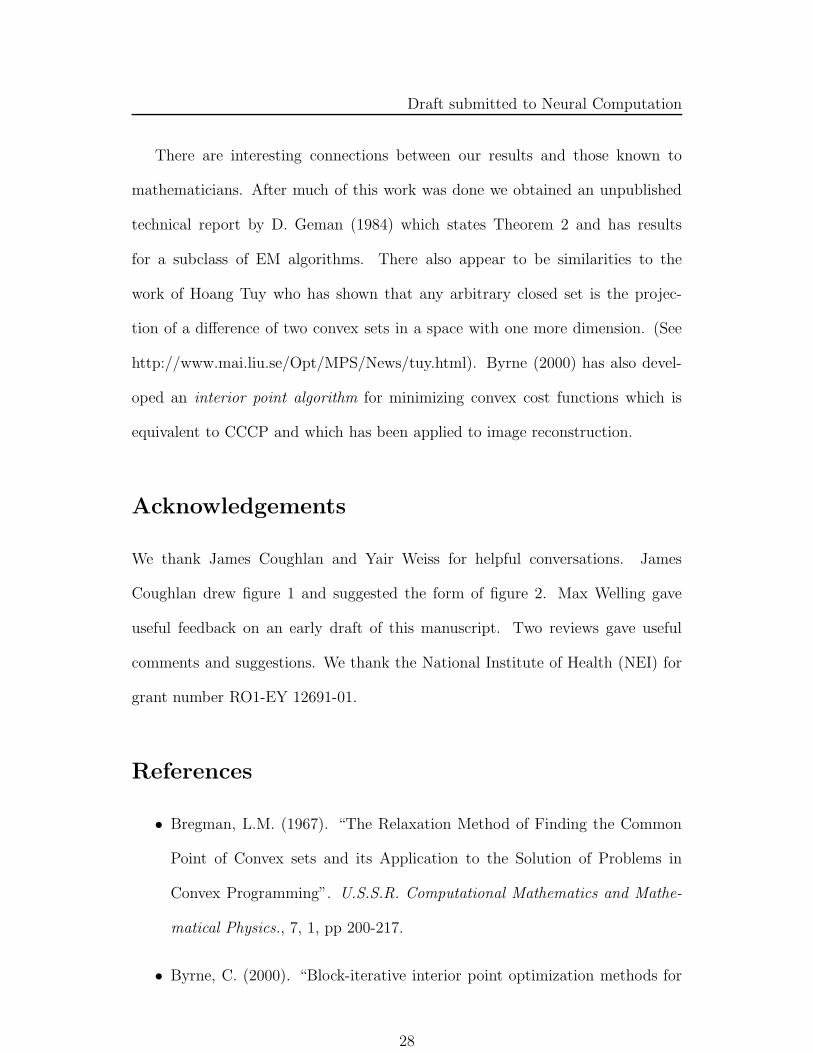
We can get a graphical illustration of this algorithm by the reformulation shown

in figure (2). Think of decomposing the energy function E(~x) into E1(~x)−E2(~x)

where both E1(~x) and E2(~x) are convex. (This is equivalent to decomposing E(~x)

into a a convex term E1(~x) plus a concave term −E2(~x)). The algorithm proceeds

by matching points on the two terms which have the same tangents. For an input

~x0 we calculate the gradient ~∇E2(~x0) and find the point ~x1 such that ~∇E1(~x1) =

~∇E2(~x0). We next determine the point ~x2 such that ~∇E1(~x2) = ~∇E2(~x1), and

repeat.

0 5 1010

20

30

40

50

60

70

0 5 100

10

20

30

40

50

60

70

80

X0 X2 X4

Figure 2: A CCCP algorithm illustrated for Convex minus Convex. We want to

minimize the function in the Left Panel. We decompose it (Right Panel) into

a convex part (top curve) minus a convex term (bottom curve). The algorithm

iterates by matching points on the two curves which have the same tangent vectors,

see text for more details. The algorithm rapidly converges to the solution at

x = 5.0.

The second statement of Theorem 2 can be used to analyze the convergence

rates of the algorithm by placing lower bounds on the (positive semi-definite)

matrix {~∇~∇Evex(~x∗) − ~∇~∇Ecave(~x

∗∗)}. Moreover, if we can bound this by a

6


matrix B then we obtain E(~xt+1) − E(~xt) ≤ −(1/2){~∇E−1vex(−~∇Ecave(~xt)) −

~xt}TB{~∇E−1

vex(−~∇Ecave(~xt))−~xt} ≤ 0, where ~∇Evex(~x)−1 is the inverse of ~∇Evex(~x).

We can therefore think of (1/2){~∇E−1vex(−

~∇Ecave(~xt))−~xt}TB{~∇E−1

vex(−~∇Ecave(~xt))−

~xt} as an auxiliary function (Della Pietra, Della Pietra, and Lafferty 1997).

We can extend Theorem 2 to allow for linear constraints on the variables

~x, for example∑

i cµi xi = αµ where the {cµ

i }, {αµ} are constants. This follows

directly because properties such as convexity and concavity are preserved when

linear constraints are imposed. We can change to new coordinates defined on the

hyperplane defined by the linear constraints. Then we apply Theorem 1 in this

coordinate system.

Observe that Theorem 2 defines the update as an implicit function of ~xt+1.

In many cases, as we will show in section (3), it is possible to solve for ~xt+1

analytically. In other cases we may need an algorithm, or inner loop, to determine

~xt+1 from ~∇Evex(~xt+1). In these cases we will need the following theorem where

we re-express CCCP in terms of minimizing a time sequence of convex update

energy functions Et+1(~xt+1) to obtain the updates ~xt+1 (i.e. at the tth iteration of

CCCP we need to minimize the energy Et+1(~xt+1)).

Theorem 3. Let E(~x) = Evex(~x) + Ecave(~x) where ~x is required to satisfy the

linear constraints∑

i cµi xi = αµ, where the {cµ

i }, {αµ} are constants. Then the

update rule for ~xt+1 can be formulated as setting ~xt+1 = arg min~x Et+1(~x) for a

time sequence of convex update energy functions Et+1(~x) defined by:

Et+1(~x) = Evex(~x) +∑

i

xi∂Ecave

∂xi

(~xt) +∑

µ

λµ{∑

i

ciµxi − αµ}, (3)

where the lagrange parameters {λµ} impose linear constraints.

Proof. Direct calculation.

The convexity of Et+1(~x) implies that there is a unique minimum ~xt+1 =

7


arg min~x Et+1(~x). This means that if an inner loop is needed to calculate ~xt+1

then we can use standard techniques such as conjugate gradient descent.

An important special case is when Evex(~x) =∑

i xi log xi. This case occurs

frequently in our examples, see section (3). We will show later in section (5) that

Et(~x) can be minimized by a CCCP algorithm.

3 Examples of CCCP

This section illustrates CCCP by examples from neural networks, mean field algo-

rithms, self-annealing (which relate to Bregman distances (Bregman 1967)), EM

and mixture models. These algorithms can be applied to a range of problems

including clustering, combinatorial optimization, and learning.

Our first example is a neural net or mean field Potts model. These have

been used for content addressable memories (Waugh and Westervelt 1993, Elfadel

1995). They have also been applied to clustering for unsupervised texture seg-

mentation (Hofmann and Buhmann 1997). An original motivation for them was

based on a convexity principle (Marcus and Westervelt 1989). We now show that

algorithms for these models can be derived directly using CCCP.

Example 1. Discrete Time Dynamical Systems for the Mean Field Potts

Model. These attempt to minimize discrete energy functions of form E[V ] =

(1/2)∑

i,j,a,b CijabViaVjb +∑

ia θiaVia, where the {Via} take discrete values {0, 1}

with linear constraints∑

i Via = 1, ∀a.

Discussion. Mean field algorithms minimize a continuous effective energy

Eeff [S; T ] to obtain a minimum of the discrete energy E[V ] in the limit as T 7→ 0.

The {Sia} are continuous variables in the range [0, 1] and correspond to (approx-

8


imate) estimates of the mean states of the {Via} with respect to the distribution

P [V ] = e−E[V ]/T /Z, where T is a temperature parameter and Z is a normaliza-

tion constant. As described in (Yuille and Kosowsky 1994), to ensure that the

minima of E[V ] and Eeff [S; T ] all coincide (as T 7→ 0) it is sufficient that Cijab

be negative definite. Moreover, this can be attained by adding a term −K∑

ia V 2ia

to E[V ] (for sufficiently large K) without altering the structure of the minima of

E[V ]. Hence, without loss of generality we can consider (1/2)∑

i,j,a,b CijabViaVjb

to be a concave function.

We impose the linear constraints by adding a Lagrange multiplier term∑

a pa{∑

i Via−

1} to the energy where the {pa} are the Lagrange multipliers. The effective energy

is given by:

Eeff [S] = (1/2)∑

i,j,a,b

CijabSiaSjb+∑

ia

θiaSia+T∑

ia

Sia log Sia+∑

a

pa{∑

i

Sia−1}.

(4)

We decompose Eeff [S] into a convex part Evex = T∑

ia Sia log Sia+∑

a pa{∑

i Sia−

1} and a concave part Ecave[S] = (1/2)∑

i,j,a,b CijabSiaSjb +∑

ia θiaSia. Taking

derivatives yields: ∂∂Sia

Evex[S] = T log Sia + pa and ∂∂Sia

Ecave[S] =∑

j,b CijabSjb +

θia. Applying CCCP by setting ∂Evex

∂Sia(St+1) = −∂Ecave

∂Sia(St) gives T{1 + log St+1

ia }+

pa = −∑

j,b CijabStjb−θia. We solve for the Lagrange multipliers {pa} by imposing

the constraints∑

i St+1ia = 1, ∀ a. This gives a discrete update rule:

St+1ia =

e(−1/T ){2∑

j,b CijabStjb

+θia}

∑

c e(−1/T ){2∑

j,b CijcbStjb

+θic}. (5)

The next example concerns mean field methods to model combinatorial opti-

mization problems such as the quadratic assignment problem (Rangarajan, Gold

and Mjolsness 1996, Rangarajan, Yuille and Mjolsness 1999) or the Travelling

9


Salesman Problem. It uses the same quadratic energy function as the last exam-

ple but adds extra linear constraints. These additional constraints prevent us from

expressing the update rule analytically and require an inner loop to implement

Theorem 3.

Example 2. Mean Field Algorithms to minimize discrete energy functions of

form E[V ] =∑

i,j,a,b CijabViaVjb+∑

ia θiaVia with linear constraints∑

i Via = 1, ∀a

and∑

a Via = 1, ∀i.

Discussion. This differs from the previous example because we need to add

an additional constraint term∑

i qi(∑

a Sia − 1) to the effective energy Eeff [S]

in equation (4) where {qi} are Lagrange multipliers. This constraint term is also

added to the convex part of the energy Evex[S] and we apply CCCP. Unlike the

previous example, it is no longer possible to express S t+1 as an analytic function of

St. Instead we resort to Theorem 3. Solving for S t+1 is equivalent to minimizing

the convex cost function:

Et+1[St+1; p, q] = T

∑

ia

St+1ia log St+1

ia +∑

a

pa{∑

i

St+1ia − 1}

+∑

i

qi{∑

a

St+1ia − 1}+

∑

ia

St+1ia

∂Ecave

Sia(St

ia). (6)

It can be shown that minimizing Et+1[St+1; p, q] can also be done by CCCP,

see section (5.3). Therefore each step of CCCP for this example requires an inner

loop which in turn can be solved by a CCCP algorithm.

Our next example is self-annealing (Rangarajan 2000). This algorithm can be

applied to the effective energies of the last two examples provided we remove the

“entropy term”∑

ia Sia log Sia. Hence self-annealing can be applied to the same

combinatorial optimization and clustering problems. It can also be applied to the

relaxation labelling problems studied in computer vision and indeed the classic

10


relaxation algorithm (Rosenfeld, Hummel and Zucker 2000) can be obtained as

an approximation to self-annealing by performing a Taylor series approximation

(Rangarajan 2000). It also relates to linear prediction (Kivinen and Warmuth

1997).

Self-annealing acts as if it has a temperature parameter which it continuously

decreases or, equivalently, as if it has a barrier function whose strength is re-

duced automatically as the algorithm proceeds (Rangarajan 2000). This relates

to Bregman distances (Bregman 1967) and, indeed, the original derivation of self-

annealing involved adding a Bregman distance to the energy function followed

by taking Legendre transforms, see section (4.2). As we now show, however,

self-annealing can be derived directly from CCCP.

Example 3. Self-Annealing for quadratic energy functions. We use the

effective energy of example 1, see equation (4), but remove the entropy term

T∑

ia Sia log Sia. We first apply both sets of linear constraints on the {Sia} (as in

example 2). Next we apply only one set of constraints (as in example 1).

Discussion. Decompose the energy function into convex and concave parts by

adding and subtracting a term γ∑

i,a Sia log Sia, where γ is a constant. This yields:

Evex[S] = γ∑

ia

Sia log Sia +∑

a

pa(∑

i

Sia − 1) +∑

i

qi(∑

a

Sia − 1),

Ecave[S] =1

2

∑

i,j,a,b

CijabSiaSjb +∑

i,a

θiaSia − γ∑

ia

Sia log Sia. (7)

Applying CCCP gives the self-annealing update equations:

St+1ia = St

iae(1/γ){−

∑

jb CijabStjb−θia−pa−qi}, (8)

where an inner loop is required to solve for the {pa}, {qi} to ensure that the con-

straints on {St+1ia } are satisfied. This inner loop is a small modification of the one

required for example 2, see section (5.3).

11


Removing the constraints∑

i qi(∑

a Sia − 1) gives us an update rule (compare

example 1):

St+1ia =

Stiae

(−1/γ){∑

jb CijabStjb

+θia}

∑

c Stice

(−1/γ){∑

jb CijbcStbj

+θic}, (9)

which, by expanding the exponential by a Taylor series, gives the equations for

relaxation labelling (Rosenfeld, Hummel and Zucker 1976) (see (Rangarajan 2000)

for details).

Our final example is the elastic net (Durbin and Willshaw 1987, Durbin,

Szeliski and Yuille 1989) in the formulation presented in (Yuille 1990). This is

an example of constrained mixture models (Jordan and Jacobs 1994) and uses an

EM algorithm (Dempster, Laird and Rubin 1977).

Example 4. The elastic net (Durbin and Willshaw 1987) attempts to solve

the Travelling Salesman Problem (TSP) by finding the shortest tour through a set

of cities at positions {~xi}. The net is represented by a set of nodes at positions

{~ya} and the algorithm performs steepest descent on a cost function E[~y]. This

corresponds to a probability distribution P (~y) = e−E[~y]/Z on the node positions

which can be interpreted (Durbin, Szeliski and Yuille 1989) as a constrained mix-

ture model (Jordan and Jacobs 1994). The elastic net can be reformulated (Yuille

1990) as minimizing an effective energy Eeff [S, ~y] where the variables {Sia} deter-

mine soft correspondence between the cities and the nodes of the net. Minimizing

Eeff [S, ~y] with respect to S and ~y alternatively can be reformulated as a CCCP

algorithm. Moreover, this alternating algorithm can also be re-expressed as an EM

algorithm for performing MAP estimation of the node variables {~ya} from P (~y),

see section (4.1).

Discussion. The elastic net can be formulated as minimizing an effective energy

12


(Yuille 1990):

Eeff [S, ~y] =∑

ia

Sia(~xi−~ya)2+γ

∑

a,b

~yTa Aab~yb+T

∑

i,a

Sia log Sia+∑

i

λi(∑

a

Sia−1),

(10)

where the {Aab} are components of a positive definite matrix representing a spring

energy and {λa} are Lagrange multipliers which impose the constraints∑

a Sia =

1, ∀ i. By setting E[~y] = Eeff [S∗(~y), ~y] where S∗(~y) = arg minS Eeff [S, ~y], we

obtain the original elastic net cost function E[~y] = −T∑

i log∑

a e−|~xi−~ya|2/T +

γ∑

a,b ~yTa Aab~yb (Durbin and Willshaw 1987). P [~y] = e−E[~y]/Z can be interpreted

(Durbin, Szeliski and Yuille 1989) as a constrained mixture model (Jordan and

Jacobs 1994).

The effective energy Eeff [S, ~y] can decreased by minimizing it with respect to

{Sia} and {~ya} alternatively. This gives update rules:

St+1ia =

e−|~xi−~yta|

2/T

∑

j e−|~xj−~yta|

2/T, (11)

∑

i

St+1ia (~yt+1

a − ~xi) +∑

b

Aab~yt+1b = 0 ∀ a, (12)

where {~yt+1a } can be computed from the {St+1

ia } by solving the linear equations.

To interpret equations (11,12) as CCCP, we define a new energy function

E[S] = Eeff [S, ~y∗(S)] where ~y∗(S) = arg min~y Eeff [S, ~y] (which can be obtained by

solving the linear equation (12) for {~ya}). We decompose E[S] = Evex[S]+Ecave[S]

where:

Evex[S] = T∑

ia

Sia log Sia +∑

i

λi(∑

a

Sia − 1),

Ecave[S] =∑

ia

Sia|~xi − ~y∗a(S)|2 + γ

∑

ab

~y∗a(S) · ~y∗

b (S)Aab. (13)

It is clear that Evex[S] is a convex function of S. It can be verified alge-

braically that Ecave[S] is a concave function of S and that its first derivative is

13


∂∂Sia

Ecave[S] = |~xi − ~y∗a(S)|2 (using the definition of ~y∗(S) to remove additional

terms). Applying CCCP to E[S] = Evex[S] + Ecave[S] gives the update rule:

St+1ia =

e−|~xi−~y∗a(St)|2

∑

b e−|~xi−~y∗b(St)|2

, ~y∗(St) = arg min~y

Eeff [St, ~y], (14)

which is equivalent to the alternating algorithm described above, see equations (11,12).

More understanding of this particular CCCP algorithm is given in the next

section where we show that is a special case of a general result for EM algorithms.

4 EM, Legendre Transforms, and Variational Bound-

ing

This section proves that two standard algorithms can be expressed in terms of

CCCP: (i) all EM algorithms, and (ii) a class of algorithms using Legendre trans-

forms. In addition, we show that CCCP can be obtained as a special case of

variational bounding and equivalent methods known as lower bound maximiza-

tion and surrogate functions.

4.1 The EM algorithm and CCCP

The EM algorithm (Dempster, Laird and Rubin 1977) seeks to estimate a variable

~y∗ = arg max~y log∑

{V } P (~y, V ), where {~y}, {V } are variables that depend on the

specific problem formulation (we will soon illustrate them for the elastic net). The

distribution P (~y, V ) is usually conditioned on data which, for simplicity, we will

not make explicit.

It was shown in (Hathaway 1986, Neal and Hinton 1998) that EM is equivalent

to minimizing the following effective energy with respect to the variables ~y and

14


P (V ):

Eem[~y, P ] = −∑

V

P (V ) log P (~y, V )+∑

V

P (V ) log P (V )+λ{∑

P (V )−1}, (15)

where λ is a lagrange multiplier.

The EM algorithm proceeds by minimizing Eem[~y, P ] with respect to P (V )

and ~y alternatively:

P t+1(V ) =P (~yt, V )

∑

V P (~yt, V ), ~yt+1 = arg min

~y−

∑

V

P t+1(V ) log P (~y, V ). (16)

These update rules are guaranteed to lower Eem[~y, P and give convergence to

a saddle point or a local minimum (Dempster, Laird and Rubin 1977, Hathaway

1986, Neal and Hinton 1998).

For example, this formulation of the EM algorithm enables us to rederive the

effective energy for the elastic net and show that the alternating algorithm is

EM. We let the {~ya} correspond to the positions of the nodes of the net and the

{Via} be binary variables indicating the correspondences between cities and nodes

(related to the {Sia} in example 4). P (~y, V ) = e−E[~y,V ]/T /Z where E[~y, V ] =

∑

ia Via|~xi − ~ya|2 + γ

∑

ab ~ya · ~ybAab with constraint that∑

a Via = 1, ∀ i. We

define Sia = P (Via = 1), ∀ i, a. Then Eem[~y, S] is equal to the effective energy

Eeff [~y, S] in the elastic net example, see equation (10). The update rules for EM,

see equation (16), are equivalent to the alternating algorithm to minimize the

effective energy, see equations (11,12).

We now show that all EM algorithms are CCCP. This requires two intermediate

results which we state as lemmas.

Lemma 1. Minimizing Eem[~y, P ] is equivalent to minimizing the function

E[P ] = Evex[P ] + Ecave[P ] where Evex[P ] =∑

V P (V ) log P (V ) + λ{∑

P (V )− 1}

15


is a convex function and Ecave[P ] = −∑

V P (V ) log P (~y∗(P ), V ) is a concave

function, where we define ~y∗(P ) = arg min~y −∑

V P (V ) log P (~y, V ).

Proof. Set E[P ] = Eem[~y∗(P ), P ], where ~y∗(P ) = arg min~y −∑

V P (V ) log P (~y, V ).

It is straightforward to decompose E[P ] as Evex[P ] + Ecave[P ] and verify that

Evex[P ] is a convex function. To determine that Ecave[P ] is concave requires

showing that its Hessian is negative semi-definite. This is performed in lemma

2.

Lemma 2. Ecave[P ] is a concave function and ∂

∂P (V )Ecave = − log P (~y∗(P ), V ),

where ~y∗(P ) = arg min~y −∑

V P (V ) log P (~y, V ).

Proof. We first derive consequences of the definition of ~y∗ which will be required

when computing the Hessian of Ecave. The definition implies:

∑

V

P (V )∂

∂~yµlog P (~y∗, V ) = 0 ∀µ (17)

∂

∂~yµlog P (~y∗, V ) +

∑

V

P (V )∑

ν

∂~y∗ν

∂P (V )

∂2

∂~yµ∂~yνlog P (~y∗, V ) = 0, ∀ µ., (18)

where the first equation is an identity which is valid for all P and the second

equation follows by differentiating the first equation with respect to P . More-

over, since ~y∗ is a minimum of −∑

V P (V ) log P (~y, V ) we also know that the

matrix∑

V P (V ) ∂2

∂yµ∂yνlog P (~y∗, V ) is negative definite. (We use the convention

that ∂∂~yµ

log P (~y∗, V ) denotes the derivative of the function log P (~y, V ) with respect

to ~yµ evaluated at ~y = ~y∗).

We now calculate the derivatives of Econv[P ] with respect to P . We obtain:

∂

∂P (V )Ecave = − log P (~y∗(P ), V )−

∑

V

P (V )∑

mu

∂~y∗µ

∂P (V )

∂ log P (~y∗, V )

∂fµ= − log P (~y∗, V ),

(19)

where we have used the definition of ~y∗, see equation (17), to eliminate the second

term on the right hand side. This proves the first statement of the theorem.

16


To prove the concavity of Ecave, we compute its Hessian:

∂2

∂P (V )∂P (V )Ecave = −

∑

ν

∂~y∗ν

∂P (V )

∂

∂~yνlog P (~y∗, V ). (20)

By using the definition of ~y∗(P ), see equation (18), we can re-express the

Hessian as:

∂2

∂P (V )∂P (V )Ecave =

∑

V,µ,ν

∂~y∗ν

∂P (V )

∂~y∗µ

∂P (V )

∂2 log P (~y∗, V )

∂~yµ∂~yν. (21)

It follows that Ecave has a negative definite Hessian and hence Ecave is concave,

recalling that −∑

V P (V ) ∂2

∂yµ∂yνlog P (~y∗, V ) is negative definite.

Theorem 4. The EM algorithm for P (~y, V ) can be expressed as a CCCP algo-

rithm in P (V ) with Evex[P ] =∑

V P (V ) log P (V )+λ{∑

P (V )−1} and Ecave[P ] =

−∑

V P (V ) log P (~y∗(P ), V ), where ~y∗(P ) = arg min~y −∑

V P (V ) log P (~y, V ). Af-

ter convergence to P ∗(V ), the solution is calculated to be ~y∗∗ = arg min~y −∑

V P ∗(V ) log P (~y, V ).

Proof. The update rule for P determined by CCCP is precisely that specified

by the EM algorithm. Therefore we can run the CCCP algorithm until it has con-

verged to P ∗(.) and then calculate the solution ~y∗∗ = arg min~y −∑

V P ∗(V ) log P (~y, V ).

Finally, we observe that D. Geman’s technical report (Geman 1984) gives

an alternative way of relating EM to CCCP for a special class of probability

distributions. He assumes that P (~y, V ) is of form e~y·~φ(V )/Z for some functions ~Φ(.).

He then proves convergence of the EM algorithm to estimate ~y by exploiting his

version of Theorem 2. Interestingly, he works with convex and concave functions

of ~y while our results are expressed in terms of convex and concave functions of

P .

17


4.2 Legendre Transformations

The Legendre transform can be used to reformulate optimization problems by

introducing auxiliary variables (Mjolsness and Garrett 1990). The idea is that

some of the formulations may be more effective and computationally cheaper

than others.

We will concentrate on Legendre minimization, see (Rangarajan, Gold and

Mjolsness 1996, Rangarajan, Yuille and Mjolsness 1999), instead of Legendre min-

max emphasized in (Mjolsness and Garrett 1990). In the later, see (Mjolsness and

Garrett 1990), the introduction of auxiliary variables converts the problem to a

min-max problem where the goal is to find a saddle point. By contrast, in Legendre

minimization, see (Rangarajan, Gold and Mjolsness 1996), the problem remains

a minimization one (and so it becomes easier to analyze convergence).

In Theorem 5 we show that Legendre minimization algorithms are equivalent

to CCCP provided we first decompose the energy into a convex plus a concave

part. The CCCP viewpoint emphasizes the geometry of the approach and com-

plements the algebraic manipulations given in (Rangarajan, Yuille and Mjolsness

1999). (Moreover, the results of this paper show the generality of CCCP while, by

contrast, Legendre transform methods have been applied only on a case by case

basis).

Definition 1. Let F (~x) be a convex function. For each value ~y let F ∗(~y) =

min~x{F (~x)+~y ·~x.}. Then F ∗(~y) is concave and is the Legendre transform of F (~x).

Two properties can be derived from this definition (Strang 1986).

Property 1. F (~x) = max~y{F∗(~y)− ~y · ~x}.

Property 2. F (.) and F ∗(.) are related by ∂F ∗

∂~y(~y) = {∂F

∂~x}−1(−~y), −∂F

∂~x(~x) =

{∂F ∗

∂~y}−1(~x). (By {∂F ∗

∂~y}−1(~x) we mean the value ~y such that ∂F ∗

∂~y(~y) = ~x.)

18


The Legendre minimization algorithms (Rangarajan, Gold and Mjolsness 1996,

Rangarajan, Yuille and Mjolsness 1999) exploits Legendre transforms. The op-

timization function E1(~x) is expressed as E1(~x) = f(~x) + g(~x) where g(~x) is

required to be a convex function. This is equivalent to minimizing E2(~x, ~y) =

f(~x) + ~x · ~y + g(~y), where g(.) is the inverse Legendre transform of g(.). Legendre

minimization consists of minimizing E2(~x, ~y) with respect to ~x and ~y alternatively.

Theorem 5. Let E1(~x) = f(~x)+g(~x) and E2(~x, ~y) = f(~x)+~x ·~y+h(~y), where

f(.), h(.) are convex functions and g(.) is concave. Then applying CCCP to E1(~x)

is equivalent to minimizing E2(~x, ~y) with respect to ~x and ~y alternatively, where

g(.) is the Legendre transform of h(.). This is equivalent to Legendre minimization.

Proof. We can write E1(~x) = f(~x) + min~y{g∗(~y) + ~x · ~y} where g∗(.) is the

Legendre transform of g(.) (identify g(.) with F ∗(.) and g∗(.) with F (.) in Defi-

nition 1 and Property 1). Thus minimizing E1(~x) with respect to ~x is equivalent

to minimizing E1(~x, ~y) = f(~x) + ~x · ~y + g∗(~y) with respect to ~x and ~y. (Alterna-

tively, we can set g∗(~y) = h(~y) in the expression for E2(~x, ~y) and obtain a cost

function E2(~x) = f(~x)+g(~x).) Alternatively minimization over ~x and ~y gives: (i)

∂f/∂~x = ~y to determine ~xt+1 in terms of ~yt, and (ii) ∂g∗/∂~y = ~x to determine

~yt in terms of ~xt which, by Property 2 of the Legendre transform is equivalent to

setting ~y = −∂g/∂~x. Combining these two stages gives CCCP:

∂f

∂~x(~xt+1) = −

∂g

∂~x(~xt).

19


4.3 Variational Bounding

In variational bounding, the original objective function to be minimized gets re-

placed by a new objective function which satisfies the following requirements, see

(Rustagi 1976, Jordan, Ghahramani, Jaakkola and Saul 1999). Other equivalent

techniques are known as surrogate functions and majorization (Lange, Hunter and

Yang 2000) or as lower bound maximization (Luttrell 1994). These techniques are

more general than CCCP and it has been shown that algorithms like EM can be

derived from them (Minka 1998, Lange, Hunter and Yang 2000). (This, of course,

does not imply that EM can be derived from CCCP).

Let E(~x), ~x ∈ RD be the original objective function that we seek to minimize.

Assume that we are at a point ~x(n) corresponding to the nth iteration. If we have

a function Ebound(~x) which satisfies the following properties, see figure (3),

E(~x(n)) = Ebound(~x(n)), and (22)

E(~x) ≤ Ebound(~x) (23)

then the next iterate ~x(n+1) is chosen such that

Ebound(~x(n+1)) ≤ E(~x(n)) whichimplies E(~x(n+1)) ≤ E(~x(n)). (24)

Consequently, we can minimize Ebound(~x) instead of E(~x) after ensuring that

E(~x(n)) = Ebound(~x(n)).

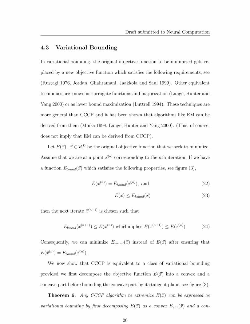
We now show that CCCP is equivalent to a class of variational bounding

provided we first decompose the objective function E(~x) into a convex and a

concave part before bounding the concave part by its tangent plane, see figure (3).

Theorem 6. Any CCCP algorithm to extremize E(~x) can be expressed as

variational bounding by first decomposing E(~x) as a convex Evex(~x) and a con-

20


Figure 3: Variational bounding, see Left Panel, bounds a function E(~x) by a

function Ebound(~x) such that E(~x(n)) = Ebound(~x(n)). We decompose E(~x) into

convex and concave parts, Evex(~x) and Ecave(~x) and bound Ecave(~x) by its tangent

plane at ~x∗, see Right Panel. We set Ebound(~x) = Evex(~x) + Ecave(~x).

cave Ecave(~x) function and then at each iteration starting at ~xt set Etbound(~x) =

Evex(~x) + Ecave(~xt) + (~x− ~xt) · ∂Ecave(~xt)

∂~x≥ Ecave(~x).

Proof. Since Ecave(~x) is concave, we have Ecave(~x∗)+(~x−~x∗)· ∂Ecave

∂~x≥ Ecave(~x)

for all ~x. Therefore Etbound(~x) satisfies the equations (22,23) for variational bound-

ing. Minimizing Etbound(~x) with respect to ~x gives ∂

∂~xEvex(~x

t+1) = −∂Ecave(~xt)∂~x

which

is the CCCP update rule.

Note that the formulation of CCCP given earlier by Theorem 3, in terms of a

sequence of convex update energy functions, is already in the variational bounding

form.

5 CCCP by changes in variables

This section gives examples where the algorithms are not CCCP in the original

variables. But they can be transformed into CCCP by changing coordinates. In

21


this section, we first show that Generalized Iterative Scaling (GIS) (Darroch and

Ratcliff 1972) and Sinkhorn’s algorithm (Sinkhorn 1964) can both be formulated

as CCCP. Then we obtain CCCP generalizations of Sinkhorn’s algorithm which

can minimize many of the inner-loop convex update energy functions defined in

Theorem 3.

5.1 Generalized Iterative Scaling

This section shows that the Generalized Iterative Scaling (GIS) algorithm (Dar-

roch and Ratcliff 1972) for estimating parameters of probability distributions can

also be expressed as CCCP. This gives a simple converge proof for the algorithm.

The parameter estimation problem is to determine the parameters ~λ of a dis-

tribution P (~x : ~λ) = e~λ·~φ(~x)/Z[~λ] so that

∑

~x P (~x;~λ)~φ(~x) = ~h, where ~h are obser-

vation data (with components indexed by µ). This can be expressed as finding the

minimum of the convex energy function log Z[λ]−~h ·~λ, where Z[~λ] =∑

~x e~λ·~φ(~x) is

the partition problem. All problems of this type can be converted to a standard

form where φµ(~x) ≥ 0, ∀ µ, ~x, hµ ≥ 0, ∀ µ, and∑

µ φµ(~x) = 1, ∀ ~x and∑

µ hµ = 1

(Darroch and Ratcliff 1972). From now on we assume this form.

The GIS algorithm is given by

λt+1µ = λt

µ − log htµ + log hµ, ∀ µ, (25)

where htµ =

∑

~x P (~x;~λt)φµ(~x). It is guaranteed to converge to the (unique)

minimum of the energy function log Z[λ] − ~h · ~λ and hence gives a solution to

∑

~x P (~x;~λ)~φ(~x) = ~h, (Darroch and Ratcliff 1972).

We now show that GIS can be reformulated as CCCP which gives a simple

convergence proof of the algorithm.

22


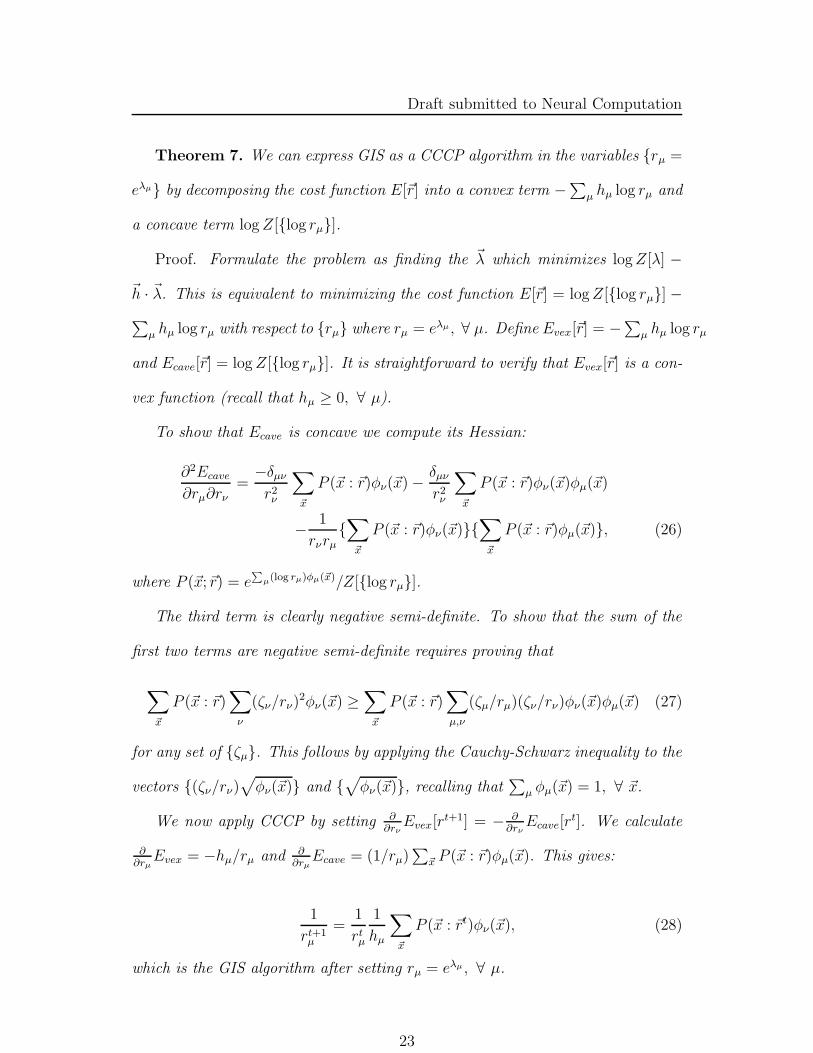
Theorem 7. We can express GIS as a CCCP algorithm in the variables {rµ =

eλµ} by decomposing the cost function E[~r] into a convex term −∑

µ hµ log rµ and

a concave term log Z[{log rµ}].

Proof. Formulate the problem as finding the ~λ which minimizes log Z[λ] −

~h · ~λ. This is equivalent to minimizing the cost function E[~r] = log Z[{log rµ}] −

∑

µ hµ log rµ with respect to {rµ} where rµ = eλµ , ∀ µ. Define Evex[~r] = −∑

µ hµ log rµ

and Ecave[~r] = log Z[{log rµ}]. It is straightforward to verify that Evex[~r] is a con-

vex function (recall that hµ ≥ 0, ∀ µ).

To show that Ecave is concave we compute its Hessian:

∂2Ecave

∂rµ∂rν=−δµν

r2ν

∑

~x

P (~x : ~r)φν(~x)−δµν

r2ν

∑

~x

P (~x : ~r)φν(~x)φµ(~x)

−1

rνrµ

{∑

~x

P (~x : ~r)φν(~x)}{∑

~x

P (~x : ~r)φµ(~x)}, (26)

where P (~x;~r) = e∑

µ(log rµ)φµ(~x)/Z[{log rµ}].

The third term is clearly negative semi-definite. To show that the sum of the

first two terms are negative semi-definite requires proving that

∑

~x

P (~x : ~r)∑

ν

(ζν/rν)2φν(~x) ≥

∑

~x

P (~x : ~r)∑

µ,ν

(ζµ/rµ)(ζν/rν)φν(~x)φµ(~x) (27)

for any set of {ζµ}. This follows by applying the Cauchy-Schwarz inequality to the

vectors {(ζν/rν)√

φν(~x)} and {√

φν(~x)}, recalling that∑

µ φµ(~x) = 1, ∀ ~x.

We now apply CCCP by setting ∂∂rν

Evex[rt+1] = − ∂

∂rνEcave[r

t]. We calculate

∂∂rµ

Evex = −hµ/rµ and ∂∂rµ

Ecave = (1/rµ)∑

~x P (~x : ~r)φµ(~x). This gives:

1

rt+1µ

=1

rtµ

1

hµ

∑

~x

P (~x : ~rt)φν(~x), (28)

which is the GIS algorithm after setting rµ = eλµ , ∀ µ.

23


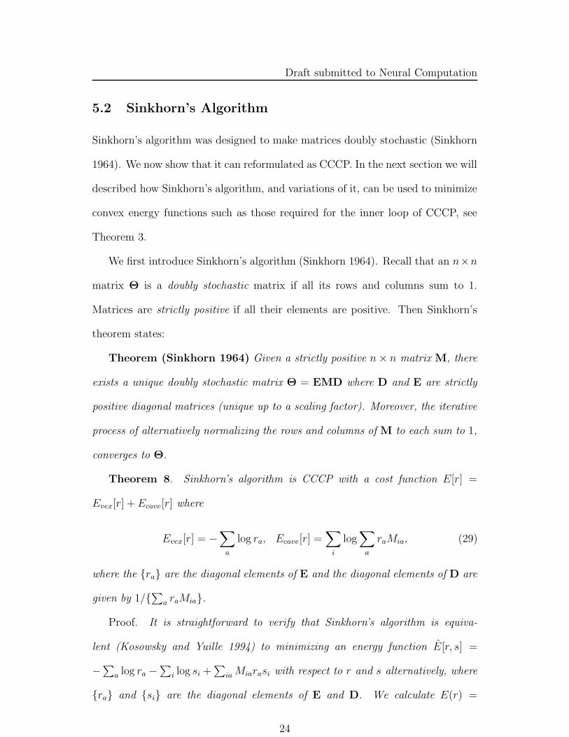
5.2 Sinkhorn’s Algorithm

Sinkhorn’s algorithm was designed to make matrices doubly stochastic (Sinkhorn

1964). We now show that it can reformulated as CCCP. In the next section we will

described how Sinkhorn’s algorithm, and variations of it, can be used to minimize

convex energy functions such as those required for the inner loop of CCCP, see

Theorem 3.

We first introduce Sinkhorn’s algorithm (Sinkhorn 1964). Recall that an n×n

matrix Θ is a doubly stochastic matrix if all its rows and columns sum to 1.

Matrices are strictly positive if all their elements are positive. Then Sinkhorn’s

theorem states:

Theorem (Sinkhorn 1964) Given a strictly positive n× n matrix M, there

exists a unique doubly stochastic matrix Θ = EMD where D and E are strictly

positive diagonal matrices (unique up to a scaling factor). Moreover, the iterative

process of alternatively normalizing the rows and columns of M to each sum to 1,

converges to Θ.

Theorem 8. Sinkhorn’s algorithm is CCCP with a cost function E[r] =

Evex[r] + Ecave[r] where

Evex[r] = −∑

a

log ra, Ecave[r] =∑

i

log∑

a

raMia, (29)

where the {ra} are the diagonal elements of E and the diagonal elements of D are

given by 1/{∑

a raMia}.

Proof. It is straightforward to verify that Sinkhorn’s algorithm is equiva-

lent (Kosowsky and Yuille 1994) to minimizing an energy function E[r, s] =

−∑

a log ra −∑

i log si +∑

ia Miarasi with respect to r and s alternatively, where

{ra} and {si} are the diagonal elements of E and D. We calculate E(r) =

24


E[r, s∗(r)] where s∗(r) = arg mins E[r, s]. It is a direct calculation that Evex[r]

is convex. The Hessian of Ecave[r] can be calculated to be

∂2

∂ra∂rbEcave[r] = −

∑

i

MiaMib

{∑

c rcMic}2, (30)

which is negative semi-definite. The CCCP algorithm is

rt+1a =

∑

i

Mia∑

c rtcMic

, (31)

which is corresponds to one step of minimizing E[r, s] with respect to r and s, and

hence is equivalent to Sinkhorn’s algorithm.

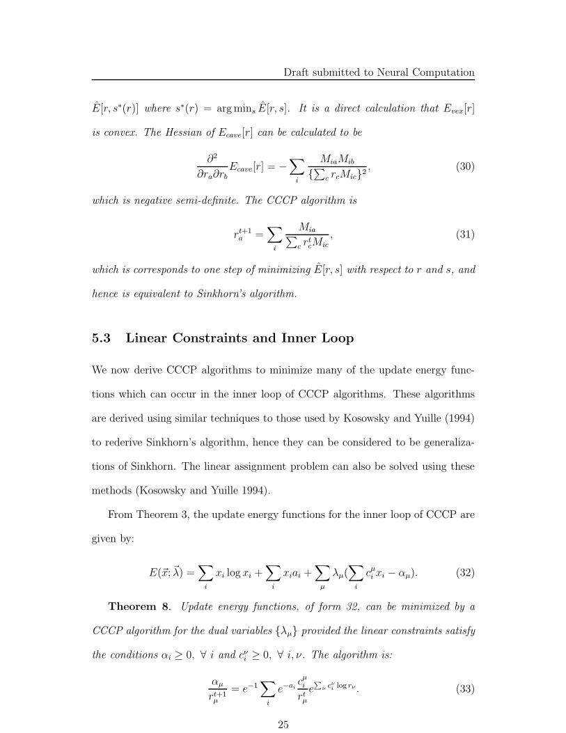
5.3 Linear Constraints and Inner Loop

We now derive CCCP algorithms to minimize many of the update energy func-

tions which can occur in the inner loop of CCCP algorithms. These algorithms

are derived using similar techniques to those used by Kosowsky and Yuille (1994)

to rederive Sinkhorn’s algorithm, hence they can be considered to be generaliza-

tions of Sinkhorn. The linear assignment problem can also be solved using these

methods (Kosowsky and Yuille 1994).

From Theorem 3, the update energy functions for the inner loop of CCCP are

given by:

E(~x;~λ) =∑

i

xi log xi +∑

i

xiai +∑

µ

λµ(∑

i

cµi xi − αµ). (32)

Theorem 8. Update energy functions, of form 32, can be minimized by a

CCCP algorithm for the dual variables {λµ} provided the linear constraints satisfy

the conditions αi ≥ 0, ∀ i and cνi ≥ 0, ∀ i, ν. The algorithm is:

αµ

rt+1µ

= e−1∑

i

e−aicµi

rtµ

e∑

ν cνi log rν . (33)

25


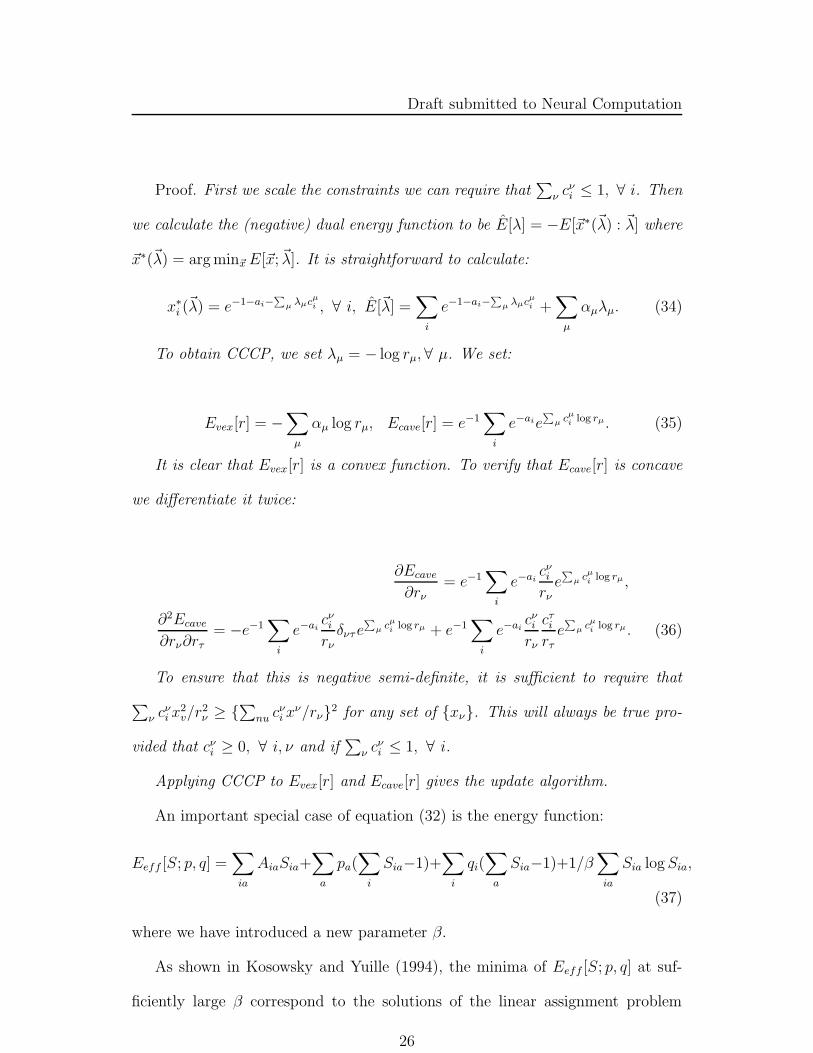
Proof. First we scale the constraints we can require that∑

ν cνi ≤ 1, ∀ i. Then

we calculate the (negative) dual energy function to be E[λ] = −E[~x∗(~λ) : ~λ] where

~x∗(~λ) = arg min~x E[~x;~λ]. It is straightforward to calculate:

x∗i (

~λ) = e−1−ai−∑

µ λµcµi , ∀ i, E[~λ] =

∑

i

e−1−ai−∑

µ λµcµi +

∑

µ

αµλµ. (34)

To obtain CCCP, we set λµ = − log rµ, ∀ µ. We set:

Evex[r] = −∑

µ

αµ log rµ, Ecave[r] = e−1∑

i

e−aie∑

µ cµi log rµ. (35)

It is clear that Evex[r] is a convex function. To verify that Ecave[r] is concave

we differentiate it twice:

∂Ecave

∂rν= e−1

∑

i

e−aicνi

rνe

∑

µ cµi

log rµ ,

∂2Ecave

∂rν∂rτ

= −e−1∑

i

e−aicνi

rν

δντe∑

µ cµi log rµ + e−1

∑

i

e−aicνi

rν

cτi

rτ

e∑

µ cµi log rµ. (36)

To ensure that this is negative semi-definite, it is sufficient to require that

∑

ν cνi x

2v/r

2ν ≥ {

∑

nu cνi x

ν/rν}2 for any set of {xν}. This will always be true pro-

vided that cνi ≥ 0, ∀ i, ν and if

∑

ν cνi ≤ 1, ∀ i.

Applying CCCP to Evex[r] and Ecave[r] gives the update algorithm.

An important special case of equation (32) is the energy function:

Eeff [S; p, q] =∑

ia

AiaSia+∑

a

pa(∑

i

Sia−1)+∑

i

qi(∑

a

Sia−1)+1/β∑

ia

Sia log Sia,

(37)

where we have introduced a new parameter β.

As shown in Kosowsky and Yuille (1994), the minima of Eeff [S; p, q] at suf-

ficiently large β correspond to the solutions of the linear assignment problem

26


whose goal is to select the permutation matrix {∏

ia} which minimizes the energy

E[∏

] =∑

ia

∏

ia Aia, where {Aia} is a set of assignment values.

Moreover, the CCCP algorithm for this case is directly equivalent to Sinkhorn’s

algorithm once we identify {e−1−βAia} with the components of M, {e−βpa} with

diagonal elements of E, and {e−βqi} with the diagonal elements of D, see statement

of Sinkhorn’s theorem. Therefore Sinkhorn’s algorithm can be used to solve the

linear assignment problem (Kosowsky and Yuille 1994).

6 Conclusion

CCCP is a general principle for constructing discrete time iterative dynamical

systems for almost any energy minimization problem. We have shown that many

existing discrete time iterative algorithms can be re-interpreted in terms of CCCP.

This includes EM algorithms, Legendre transforms, Sinkhorn’s algorithm, and

Generalized Iterative Scaling. Alternatively, CCCP can be seen as a special case

of variational bounding, lower bound maximization (upper bound minimization),

and surrogate functions. CCCP gives a novel geometrical way for understanding,

and proving convergence of, existing algorithms.

Moreover, CCCP can also be used to construct novel algorithms. See, for

example, recent work (Yuille 2002) where CCCP was used to construct a double

loop algorithm to minimize the Bethe/Kikuchi free energy (Yedidia, Freeman,

and Weiss 2000). CCCP is a design principle and does not specify a unique

algorithm. Different choices of the decomposition into convex and concave parts

will give different algorithms with, presumably, different convergence rates. It is

interesting to explore the effectiveness of different decompositions.

27


There are interesting connections between our results and those known to

mathematicians. After much of this work was done we obtained an unpublished

technical report by D. Geman (1984) which states Theorem 2 and has results

for a subclass of EM algorithms. There also appear to be similarities to the

work of Hoang Tuy who has shown that any arbitrary closed set is the projec-

tion of a difference of two convex sets in a space with one more dimension. (See

http://www.mai.liu.se/Opt/MPS/News/tuy.html). Byrne (2000) has also devel-

oped an interior point algorithm for minimizing convex cost functions which is

equivalent to CCCP and which has been applied to image reconstruction.

Acknowledgements

We thank James Coughlan and Yair Weiss for helpful conversations. James

Coughlan drew figure 1 and suggested the form of figure 2. Max Welling gave

useful feedback on an early draft of this manuscript. Two reviews gave useful

comments and suggestions. We thank the National Institute of Health (NEI) for

grant number RO1-EY 12691-01.

References

• Bregman, L.M. (1967). “The Relaxation Method of Finding the Common

Point of Convex sets and its Application to the Solution of Problems in

Convex Programming”. U.S.S.R. Computational Mathematics and Mathe-

matical Physics., 7, 1, pp 200-217.

• Byrne, C. (2000). “Block-iterative interior point optimization methods for

28


image reconstruction from limited data.” Inverse Problem. 14, pp 1455-

1467.

• Darroch, J.N. and Ratcliff, D. (1972). “Generalized Iterative Scaling for

Log-Linear Models”. The Annals of Mathematical Statistics. Vol. 43. No.

5, pp 1470-1480.

• Della Pietra, S., Della Pietra, V. and Lafferty, J. (1997). “Inducing features

of random fields”. IEEE Transactions on Pattern Analysis and Machine

Intelligence. 19(4), pp 1-13.

• Dempster, A.P., Laird, N.M. and Rubin, D.B. (1977). “Maximum likeli-

hood from incomplete data via the EM algorithm.” Journal of the Royal

Statistical Society, B, 39, 1-38.

• Durbin, R., Willshaw, D. (1987). ”An Analogue Approach to the Travelling

Salesman Problem Using an Elastic Net Method”, Nature, v.326, n.16, ,

p.689.

• Durbin, R., Szeliski, R. and Yuille, A.L. (1989).“ An Analysis of an Elastic

net Approach to the Traveling Salesman Problem”. Neural Computation.

1, pp 348-358.

• Elfadel, I.M. (1995). “Convex potentials and their conjugates in analog

mean-field optimization”. Neural Computation. Volume 7. Number 5. pp.

1079-1104.

• Geman, D. (1984). “Parameter Estimation for Markov Random Fields with

Hidden Variables and Experiments with the EM Algorithm”. Working Pa-

29


per no. 21. Dept. Mathematics and Statistics. University of Massachusetts

at Amherst.

• Hathaway, R. (1986). “Another Interpretation of the EM Algorithm for

Mixture Distributions”. Statistics and Probability Letters. Vol. 4, pp 53-56.

• Hofmann, T. and Buhmann, J.M. (1997). “Pairwise Data Clustering by De-

terministic Annealing”. IEEE Transactions on Pattern Analysis and Ma-

chine Intelligence (PAMI), 19(1), 1-14.

• Jordan, M.I. and Jacobs, R.A. (1994). “Hierarchical mixtures of experts

and the EM algorithm”. Neural Computation, 6, 181–214.

• Jordan, M.I., Ghahramani, Z. and Jaakkola, T.S. and Saul, L.K. (1999).

“An introduction to variational methods for graphical models”. Machine

Learning 37, pp 183-233.

• Kivinen, J. and Warmuth, M. (1997). “Additive versus Exponentiated Gra-

dient Updates for Linear Prediction”. J. Inform. Comput. 132 (1), pp

1-64.

• Kosowsky, J.J. and Yuille, A.L. (1994). “The Invisible Hand Algorithm:

Solving the Assignment Problem with Statistical Physics”. Neural Net-

works., Vol. 7, No. 3, pp 477-490.

• Lange K, Hunter D.R., Yang, I. (2000). ”Optimization transfer using surro-

gate objective functions” (with discussion), Journal of Computational and

Graphical Statistics, 9: 1-59.

• Luttrell, S.P. (1994). “Partitioned mixture distributions: an adaptive bayesian

30


network for low-level image processing.” IEEE Proceedings on Vision, Im-

age and Signal Processing. 141(4): 251-260.

• Marcus, C. and Westervelt, R.M. (1989). “Dynamics of Iterated-Map Neural

Networks”. Physics Review A. 40, pp 501-509.

• Minka, T.P. (1998). “Expectation-Maximization as lower bound maximiza-

tion”. Technical Report. Available from http://www.stat.cmu.edu/ minka/papers/learning.html.

• Mjolsness, E. and Garrett, C. (1990). “Algebraic Transformations of Objec-

tive Functions”. Neural Networks. Vol. 3, pp 651-669.

• Neal, R.M. and Hinton, G.E. (1998). A view of the EM algorithm that

justifies incremental, sparse, and other variants. In Learning in Graphical

Model M.I. Jordan (editor).

• Press, W.H., Flannery, B.R., Teukolsky, S.A. and Vetterling, W.T. (1986).

Numerical Recipes. Cambridge University Press.

• Rangarajan, A., Gold, S. and Mjolsness, E. (1996). “A Novel Optimizing

Network Architecture with Applications”. Neural Computation, 8(5), pp

1041-1060.

• Rangarajan, A. Yuille, A.L. and Mjolsness, E. (1999). ”A Convergence Proof

for the Softassign Quadratic Assignment Algorithm”. Neural Computation.

11, pp 1455-1474.

• Rangarajan, A. (2000). “Self-annealing and self-annihilation: unifying de-

terministic annealing and relaxation labeling”. Pattern Recognition. Vol.

33, pp 635-649.

31


• Rosenfeld, A., Hummel,R, and Zucker, S. (1976). “Scene Labelling by Re-

laxation Operations”. IEEE Trans. Systems MAn Cybernetic. Vol 6(6), pp

420-433.

• Rustagi,J. (1976). Variational Methods in Statistics. Academic Press.

• Strang, G. (1986). Introduction to Applied Mathematics. Wellesley-

Cambridge Press. Wellesley, Massachusetts.

• Sinkhorn, R. (1964). “A Relationship Between Arbitrary Positive Matrices

and Doubly Stochastic Matrices”. Ann. Math. Statist.. 35, pp 876-879.

• Waugh, F.R. and Westervelt, R.M. (1993). “Analog neural networks with

local competition: I. Dynamics and stability”. Physical Review E, 47(6), pp

4524-4536.

• Yuille, A.L. (1990). “Generalized Deformable Models, Statistical Physics

and Matching Problems,” Neural Computation, 2 pp 1-24.

• Yuille, A.L. and Kosowsky, J.J. (1994). “Statistical Physics Algorithms that

Converge.” Neural Computation. 6, pp 341-356.

• Yedidia, J.S., Freeman, W.T. and Weiss, Y. (2000). “Bethe free energy,

Kikuchi approximations and belief propagation algorithms”. Proceedings of

NIPS’2000.

• Yuille, A.L. (2002). “A Double-Loop Algorithm to Minimize the Bethe and

Kikuchi Free Energies”. Neural Computation. In press.

32

Documents

The Concave-Convex Procedure (CCCP)