The content is identical to the content of the published ... · d’expériences optimaux pour la calibration d’un modèle de la microbiologie prédictive Dries Telen 1, Filip Logist

This document contains the post-print pdf version of the refereed paper: “On the trade-off between experimental effort and information content in optimal experimental design for calibrating a predictive microbiology model” by Dries Telen, Filip Logist, Eva Van Derlinden and Jan Van Impe

which has been archived on the university repository Lirias (https://lirias.kuleuven.be/) of the KU Leuven. The content is identical to the content of the published paper, but without the final typesetting by the publisher. When referring to this work, please cite the full bibliographic info:

D. Telen, F. Logist, E. Van Derlinden and J. Van Impe (2013). On the trade-off between experimental effort and information content in optimal experimental design for calibrating a predictive microbiology model, Journal de la Societe Francaise de Statistique, 154(3), 95-112. http://www.sfds.asso.fr/34-Journal_de_la_SFdS_J_SFdS http://journal-sfds.fr/index.php/J-SFdS/ The corresponding author can be contacted for additional info. Conditions for open access are available at: http://www.sherpa.ac.uk/romeo/

https://lirias.kuleuven.be/

http://www.sfds.asso.fr/34-Journal_de_la_SFdS_J_SFdS

http://journal-sfds.fr/index.php/J-SFdS/

http://www.sherpa.ac.uk/romeo/

Postprint version of paper published in JSFS 2014, vol. 154(3), p. 95–112. The content is identical to the published paper, but without the final typesetting by the publisher.

Journal homepage: http://www.sfds.asso.fr/34-Journal_de_la_SFdS_J_SFdS Original file available at: http://journal-sfds.fr/index.php/J-SFdS/

Submission

Journal de la Société Française de Statistique

On the trade-off between experimental effort andinformation content in optimal experimental design

for calibrating a predictive microbiology modelTitre: Sur le compromis entre l’effort expérimental et le contenu des informations dans les plans

d’expériences optimaux pour la calibration d’un modèle de la microbiologie prédictive

Dries Telen 1 , Filip Logist 1 , Eva Van Derlinden 1 and Jan Van Impe 1

Abstract: In predictive microbiology, dynamic mathematical models are developed to describe microbial evolutionunder time-varying environmental conditions. Next to an acceptable model structure, reliable parameter values arenecessary to obtain valid model predictions. To obtain these accurate estimates of the model parameters, labor-andcost-intensive experiments have to be performed. Optimal experimental design techniques for parameter estimationare beneficial to limit the experimental burden. An important issue in optimal experimental design, included in thiswork, is the sampling scheme. Recent work illustrates that identifying sampling decisions results in bang-bang controlof the weighting function in the Fisher information matrix. A second point addressed in this work is the trade-offbetween the amount of time an experimenter has available for measurements on the one hand, and information contenton the other hand. Recently, multi-objective optimization is applied to several different optimal experimental designcriteria, whereas in this paper the workload expressed as when to sample, is considered. The procedure is illustratedthrough simulations with a case study for the Cardinal Temperature Model with Inflection. The viability of the obtainedexperiments is assessed by calculating the confidence regions with two different methods: the Fisher informationmatrix approach and the Monte-Carlo method approach.

Résumé :Aujourd’hui, dans le domaine de la microbiologie prédictive, la croissance et la décroissance des populations

bactériennes sont décrites par des modèles mathématiques dynamiques, dits primaires. Les paramètres de ces modèlesprimaires sont eux-mêmes liés à des facteurs environnementaux par des modèles, dits secondaires, comprenantplusieurs paramètres secondaires (typiquement des températures et des pH minimaux, maximaux et optimaux). A cettecomplexité hiérarchique des modèles s’ajoutent inéluctablement de nombreuses sources d’erreurs de mesure comptetenu de la nature biologique des objets expérimentaux, erreurs qui affectent les observations issues des expériences demicrobiologie. A l’évidence, il est donc particulièrement crucial de disposer de protocoles expérimentaux performants,qui prennent en compte à la fois ces structures de modèles et les erreurs, pour conduire in fine à des estimations dequalité (faible biais, faible variance, ...) des paramètres secondaires, et aussi à des prédictions fiables avec les modèlesestimés. Même s’il existe plusieurs critères d’optimalité pour construire de tels protocoles performants, le coût de leurmise en oeuvre reste toutefois souvent prohibitif de par le nombre d’essais expérimentaux à réaliser. Dans cet article,deux nouvelles approches sont proposées dans un cadre de critères d’optimalité de plans d’expériences bien connus :a) un schéma d’échantillonnage temporel formalisé par une fonction de pondération de type "tout ou rien" ajoutéedans la forme dynamique de la fonction d’information de Fisher ; cette fonction va permettre à l’expérimentateur dedécider si on doit échantillonner ou non à un temps donné optimisé (effort expérimental), et b) l’élaboration d’uncompromis entre l’effort expérimental à fournir, commandé par le protocole optimal, et le contenu de l’informationobtenue grâce à ce protocole ; cette élaboration est basée sur l’utilisation de techniques d’optimisation multi-objectifs.

1 BioTeC & OPTEC - Chemical and Biochemical Process Technology and ControlDepartment of Chemical Engineering, KU LeuvenW. de Croylaan 46, B-3001, Leuven, Belgium.E-mail: [email protected]

Soumis au Journal de la Société Française de StatistiqueFile: jsfds_Telen_unmarkedv2.tex, compiled with jsfds, version : 2009/12/09date: July 22, 2013



2 Telen, Logist, Van Derlinden and Van Impe

Usuellement, quand ces techniques sont utilisées pour déterminer un protocole optimal, l’effort expérimental n’est paspris en compte. Enfin, à partir d’un modèle bien connu des microbiologistes, des simulations ont été menées à la foispour évaluer la faisabilité des protocoles calculés et déterminer des intervalles de confiance pour les estimations desparamètres.Keywords: optimal experimental design, multi-objective optimization, parameter estimation, Monte-Carlo simulationMots-clés : plan d’expériences optimal, optimisation multi-objectif, l’estimation paramétrique, méthode de Monte-Carlo

1. Introduction

Dynamic models that predict microbial behavior in food products play an important role in foodquality and safety. In these models, the effect of temperature, pH, water activity and preservativesare important elements. When a suitable model structure is chosen, reliable parameter estimateshave to be obtained for different microbial strains. However, performing experiments is cost- andlabor-intensive. The experimenter must take samples and, subsequently, perform an extensiveanalysis procedure. To reduce this experimental effort, optimal experimental design (OED) canbe applied. In optimal experimental design for parameter estimation, some scalar function of theFisher information matrix [23, 34] is employed as objective function in the resulting dynamicoptimization problem. Design of an optimal experimental can focus on different aspects.

The main contribution is a practical procedure for systematically evaluating trade-offs betweeninformation content and experimental effort in the design of dynamic experiments for calibratingpredictive microbiology models. Advanced multi-objective dynamic optimization approaches areexploited with parameter accuracy and total time reserved for measuring as specific (conflicting)objectives. With respect to the latter objective, the determination of optimal measurement/samplingschemes specifying when to measure, is added as a degree of freedom.

Recent work discussing when to sample [25] indicates that the inclusion of the weighting functionin the Fisher information matrix results in a bang-bang type control [25, 22]. Bang-bang control isa type of control which arises in optimal control when the optimal value for the control action iseither at its minimum or maximum value. The necessary conditions for the existence/occurrenceof this type of control can be found in, e.g., [28]. The maximal amount of measurement time is nota priori fixed and not necessarily equal to the experiment duration, but is added as an additionalobjective to be minimized.

To enable an overview of the trade-offs, multi-objective optimization is exploited to generate theset of Pareto optimal solutions, which contains different optimal alternatives. This availability ofthe Pareto set allows the experimenter to make a sound decision based on his/her preferences. Assuch, the presented procedure is an extension to the work of [29] as it integrates strategies from[25].

The accuracy of the designed experiments with reduced workload is assessed in a simulationstudy for the Cardinal Temperature Model with Inflection (CTMI), which describes the effectof temperature on the microbial growth rate. Based on generated data, a parameter estimationprocedure is carried out and confidence intervals are calculated. A first approach exploits the




Trade-off between experimental effort and information content 3

Fisher information matrix. However, one known drawback of this matrix is that, for modelsnon-linear in the parameters [1, 12, 27], it can result in inaccurate estimates of the confidenceintervals. Hence, to check the validity of the Fisher information matrix approach for the CTMImodel, a Monte-Carlo simulation [34] is also performed.

The paper is structured as follows. In Section 2, the employed mathematical techniques andthe mathematical model are discussed. Section 3 presents the obtained results. Afterwards, inSection 4, the conclusions are formulated.

2. Methods and Model

Optimal experimental design for dynamic models gives rise to a specific subclass of dynamicoptimization problems. The general concept of dynamic optimization and the techniques ofoptimal experimental design are discussed in the first part of this section. Because samplingschemes are considered in this paper, recent work on sampling decisions is discussed in thesecond part. As no single optimal criterion for optimal experimental design exists, conflictingcriteria can be considered by employing multi-objective optimization [29]. Hence, the specificmethods of multi-objective optimization are described in the third part. The fourth part discussesthe validation process of the computation of the confidence intervals. In the last subsection, thepredictive microbiological case study is presented.

2.1. Optimal experimental design

An adequately general formulation of a dynamic optimization problem for the purpose of thispaper, reads as follows:

minx(t),u(t)

J(x(t),u(t),p, t) (1)

subject to:

dxdt

= f(x(t),u(t),p, t) (2)

0 = bc(x(0)) (3)

0 ≥ cp(x(t),u(t),p, t) (4)

0 ≥ ct(x(t f ),u(t f ),p, t f ) (5)

where t is the time in the interval [0, t f ], x are the state variables, u are the control variables andp the parameters. The dynamic system equations are represented by f. The vector bc indicatesthe initial conditions, the vector cp the path inequality constraints and the vector ct the terminalinequality constraints on controls and states. Furthermore, the vector y containing the measuredoutputs, is introduced. These are usually a subset of the state variables x. The degrees of freedomsof the optimal experimental design are grouped in a vector of trajectories z = [x(t)T ,u(t)T ]T . Allvectors z that satisfy equations (2) to (5) form the set of feasible solutions S.

This optimization problem is infinite-dimensional. These problems are solved within this work





by converting them to a finite Non-Linear Programming (NLP) problem by means of discretiza-tion. There are two different approaches. A sequential direct method as single shooting (e.g.,[26, 32, 33]) discretizes only the controls u using piecewise polynomials. The differential equa-tions are subsequently solved using standard integrators and the objective function is evaluated.The parametrized controls are updated using a standard optimization algorithm. Alternatively,simultaneous direct methods discretize both states and controls. The simulation and optimizationare performed simultaneously which results in larger NLPs than in the sequential approach. Twodifferent approaches exist within the class of simultaneous direct methods: multiple shooting (e.g.,[6, 14]) and orthogonal collocation (e.g., [3, 4]). In multiple shooting, the integration range issplit in a finite number of intervals while in orthogonal collocation the states are fully discretizedbased on orthogonal polynomials. These large NLPs require tailored algorithms that exploit theproblems’ structure and sparsity. In view of brevity, the interested reader is referred to [5] for ageneral overview and discussion.

In optimal experimental design for parameter estimation, a scalar function Φ(.) of the Fisherinformation matrix is used as the objective function. This matrix is defined as:

F(p) =∫ t f

0

(∂y(p, t)

∂p

)T ∣∣∣∣p=p∗

Q(

∂y(p, t)∂p

)∣∣∣∣p=p∗

dt (6)

The true values p∗ are unknown so the Fisher matrix depends on their current best estimate. Twoparts constitute the Fisher information matrix: the matrix Q, being the inverse of the measurementerror variance-covariance matrix and ∂y(p,t)

∂p , the sensitivities of the model output with respect tosmall variations in the model parameters. The latter can be found as the solution to:

ddt

∂y(p, t)∂p

=∂ f∂y

∂y(p, t)∂p

+∂ f∂p

(7)

An interesting property of the Fisher information matrix is that under the assumption of unbiasedestimators, the inverse of F is the lower bound of the parameter estimation variance-covariancematrix, i.e., the Cramér-Rao lower bound [15].

The matrix F contains the information of a specific experiment. To optimize this amount ofinformation a scalar function of F has to be selected as the optimization problem’s objectivefunction. Mathematically this is expressed as:

J = Φ(F(x(t),u(t),p, t)) (8)

where Φ(.) is one of the criteria further described. The most widely used scalar functions arelisted below [23, 34, 10].

• A-criterion: min[trace(F−1)] A-optimal designs minimize the mean of the asymptotic vari-ances of individual parameter estimates. The geometrical interpretation is the minimizationof the enclosing frame around the joint confidence region.

• D-criterion: max[det(F)] D-optimal designs minimize the geometric mean of the eigen-values of the approximate variance-covariance matrix. Geometrically, this is minimizingthe volume of the joint confidence region. Note that when only a subset of the parametersare considered, this is the Ds-criterion [34].





• E-criterion: max[λmin (F)] E-optimal designs aim at minimizing the largest asymptoticvariance of individual parameter estimates. This corresponds to minimizing the length ofthe largest uncertainty axis of the joint confidence region.

2.2. Determination of an optimal sampling scheme

In [25], an additional control function ν(t) ∈ [0,1] is introduced in the Fisher information matrix,which is then defined as:

F(p) =∫ t f

0ν(t)

(∂y(p, t)

∂p

)T ∣∣∣∣p=p∗

Q(

∂y(p, t)∂p

)∣∣∣∣p=p∗

dt (9)

This function ν(t) is a binary function indicating whether or not measurements are required attime t. Mathematically this is expressed as v(t) ∈ {0,1} ∀t ∈ [0, t f ]. Note that in the current papermeasuring several times at the same time instance is excluded. However, to provide a tractableoptimal control problem, the problem is relaxed to ν(t)∈ [0,1] and the strategy described in [25] isfollowed. Note that there is a subtle difference between the experiment time and the measurementtime. The experiment time is assumed to be a predetermined number of hours. The measurementtime is the amount of hours the experimenter is willing to spend to take measurements. Thisvalue is assumed not to be set a priori. The measurement time can of course never exceed thetotal experiment time. When the measurement time is not constrained to a certain value, themaximum information content is found by measuring continuously during the experiment time.As performing experiments is cost-and labor-intensive, the following additional objective is takeninto consideration:

minν(t)

W (10)

in which:dWdt

= ν(t) (11)

W (0) = 0 (12)

This objective represents the experimental/measurement effort in the sense that it representsthe total amount of hours spent measuring during the experiment. This objective can also beformulated as a constraint W (t f ) ≤ α ≤ t f in a single objective optimization problem. Thisproblem formulation closely resembles the work of [9]. In the latter work, a numerical procedurefor optimal design is presented based on the idea to delete less informative sets and to includemore informative ones at every step of the procedure. Furthermore, the idea that the total amountof measurements is constrained to an a priori specified value is also present and equivalent to theapproach in the current paper. However, the difference is that the current paper does not requirethe model to be linear in the parameters, which is one of the assumptions in [9]. This means thatthe Fisher information matrix depends on the best estimates of the parameters and no guarantee onglobal optimality of the design can be provided. Note that, in the current work, the experimentaleffort is computed as the time integral of the measurement time. This approach can be generalizedby taking the integral of a different function (e.g., computing the financial cost) by taking intoaccount the cost to take samples at different points.





2.3. Multi-objective optimization

The formulation of a dynamic optimization problem involving multiple objectives J1 to Jm isdescribed as:

minz{J1(z), . . . ,Jm(z)} (13)

subject to equations (2) to (5).

In multi-objective optimization, Pareto optimality is used (see, e.g., [21]). A solution is calledPareto optimal if there exists no other feasible solution that improves at least one objectivefunction without worsening another. The decision variables z belong to the feasible set S, de-fined previously, and the vector of all individual cost functions is defined as J = [J1(z), . . . ,Jm(z)]T.

The (convex) weighted sum (WS) is in practice the most widely-used technique for combiningdifferent objectives. By consistently varying the weights assigned to each cost Ji an approxima-tion of the Pareto set is obtained. However, despite its simplicity, the weighted sum has severalintrinsic drawbacks [7]: a uniform distribution of the weights does not necessarily result in aneven spread on the Pareto front, and points in non-convex parts of the Pareto set cannot be obtained.

Two recent scalarization-based multi-objective optimization techniques are the normal boundaryintersection (NBI) [8] and the (enhanced) normalized normal constraint ((E)NNC) [20]. Bothtechniques mitigate the discussed disadvantages of the WS and allow the use of fast gradient-based solvers. For a more detailed description of the NBI and (E)NNC, the interested reader isreferred to [16, 19]. In recent, work a connection [19] between the WS, NBI and (E)NNC is proven.

In [25], a different approach is presented to make the trade-off between experimental effort andinformation gain. The author suggests adding a linear penalty of the control ν(t) to the objective.In this penalty term, there is a factor ε which is shown to be a minimum bound on the informationgain. As this ε is set a priori this approach leads to a single optimal solution in a similar manneras fixing the total amount of measurement time which is equivalent to the ε-constraint method[11]. The authors of the current paper prefer to solve this trade-off in a multi-objective frameworkto ensure the experimenter can make an informed decision.

2.4. Validation of the confidence regions

To assess the viability of the obtained experiments, simulations with pseudo-measurements areperformed for different workload settings. To this extent, random white noise is added to theexpected state evolution. This noise is drawn from a normal distribution with zero mean and avariance equal to the state measurement variance, σ2

n .

To estimate the confidence intervals, the approximate variance-covariance matrix C is calcu-lated parameter estimation. The individual confidence intervals of the parameters are givenas:

pi± tnt−npα/2

√Cii (14)





where tnt−npα/2 is the upper critical value of the Student’s t-distribution with tolerance level α and

nt −np degrees of freedom, nt is the number of measurements, np is the number of parametersand α is the (1−α)100% confidence level employed by the user.

The model under study is non-linear in the parameters. As a result, the parameter estimationmay yield an inaccurate estimation of the real confidence region [1, 12, 27]. In order to assessthe viability of the obtained confidence regions, a Monte-Carlo-analysis is performed [34]. Inthis work, 500 pseudo-measurement sets are generated. For each set, the model parameters areidentified. Next, the 95% empirical confidence bounds on the parameters pi are computed.

2.5. Predictive microbial growth model for E. coli

In this case study, optimal experiments for identifying the parameters of the Cardinal TemperatureModel with Inflection (CTMI) [24] are designed. This is a secondary model to the model ofBaranyi and Roberts [2]. This latter model describes the cell density as a function of time whilethe former incorporates the dependency on temperature. The model equations of the Baranyi andRoberts model are:

dn(t)dt

=Q(t)

Q(t)+1µmax(T (t))[1− exp(n(t)−nmax)] (15)

dQ(t)dt

= µmax(T (t))Q(t) (16)

with the states x(t) = [n(t) Q(t)]T . The state n(t) [ln(CFU/ml)] is the natural logarithm of the celldensity and Q(t) [-] the physiological state of the cells. The observable state is y(t) = n(t). Thecontrol input to this system is the temperature profile u(t) = T (t). The temperature dependencyof the CTMI is given by:

µmax = µoptγ(T (t)) (17)

with:

γ(T (t)) =(T (t)−Tmin)2(T (t)−Tmax)

(Topt −Tmin)[(Topt −Tmin)(T (t)−Topt)− (Topt −Tmax)(Topt +Tmin−2T (t))](18)

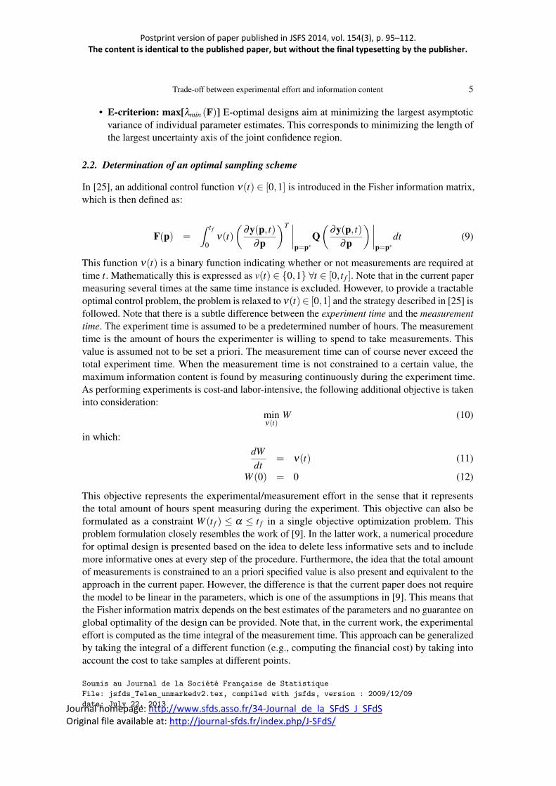
The values of the parameters p = [µmax Tmin Topt Tmax]T for the model [31] are shown in Table 1.The Cardinal Temperature Model with Inflection is illustrated in Figure 1. Tmin is the minimaltemperature needed for growth, Tmax is the maximal temperature where growth can occur. In caseof temperatures lower than Tmin or higher than Tmax, no growth is assumed. Topt is the temperatureat which the growth rate µ is optimal. When designing experiments, the end time is fixed to 38 h[31]. For model validity reasons the dynamic temperature profiles are constrained to:

15◦C≤ T (t) ≤ 45◦C (19)

−5◦C/h≤ dT (t)/dt ≤ 5◦C/h (20)

The temperature profile is designed as a combination of piecewise linear parts [31] to ensurepractical implementation. The simplest approach is to estimate the four parameters from one





FIGURE 1. Cardinal Temperature Model with Inflection with illustration of the meaning of the four parameters.

single experiment. In previous work, the following practical strategy was proposed and validatedexperimentally. The four parameters are divided in six 2-parameter combinations ((Tmax,µopt),(Tmax,Tmin), (Tmax,Topt), (Tmin,µopt), (Tmin,Topt) and (Topt ,µopt)) and for each combination anoptimal experiment was designed. By only considering two parameters, the Ds-criterion is actuallyused instead of the D-criterion [34]. Although the four parameters are unknown, only two areof interest in the design while the others are considered nuisance. Note that Ds-designs can besingular. By performing these six experiments, each individual parameter is considered threetimes (with each of the other parameters). This approach increases the experimental load, butwas chosen as an acceptable trade-off with respect to parameter accuracy [30, 31]. In [31] it wasillustrated on simulation level that four 2-parameter combinations lead to an acceptable level ofparameter accuracy provided each individual parameter is considered twice in two combinations.Note that three such possible combinations exist. To enable a fair comparison, the strategy ofdividing into six 2-parameter combinations is also followed in this work.

TABLE 1. Parameter values used for the design of the optimal experiments for the predictive growth model.

Tmin 11.33 ◦C Topt 40.85 ◦CTmax 46.54 ◦C µopt 2.397 1/hnmax 22.55 ln(CFU/mL) σ2

n 3.27×10−2 ln(CFU/mL)2

3. Results

In the first subsection, the individual results for the different parameter combinations are discussed.The trade-off between the experimental burden and the information content is discussed in thesecond subsection. The third subsection presents the discussion of the parameter accuracy.





3.1. Maximizing information content

In order to estimate the four model parameters, six possible two-parameter combinations canbe used. For each combination, the corresponding cost function is optimized using the Ds-criterion [31]. The six criteria as used in [31] are: J1 = DsTmax,µopt , J2 = DsTmax,Tmin , J3 = DsTmax,Topt ,J4 = DsTmin,µopt , J5 = DsTmin,Topt , J6 = DsTopt ,µopt . The individual maxima are summarized in Table2. These values are obtained using a multiple shooting [6] approach using the ACADO-toolkit[13] which allows for a fast computation of the optimal profiles. The integrator tolerance of theRungeKutta78 and the KKT-tolerance of the resulting SQP-problem are set to 10−6. In this case,the assumption is that the measurements are performed continuously during the 38 hours of theexperiment. These results are used as initialization in the next section as they represent the upperbound of available information content. The results in Table 2 are similar to those in [31]. Itshould be noted that the employed non-linear programming does not guarantee global optimality,only local optimality is ensured. The effect of increasing the number of discretization intervals isclearly visible in Table 2. The third column depicts the results for a different control action everyfifteen minutes whereas the second column requires a control action every two hours. By a finercontrol discretization, slightly better results are obtained. However, nineteen control intervalswill be chosen in the subsequent simulations to limit computational time. Compared with theapproach in [31], there are more degrees of freedom in this paper. In [31] the temperature profileis constrained to two constant phases and a connecting linear section. The degrees of freedom in[31] are: the initial temperature profile, the switching time to start the linear phase, the slope ofthe linear phase and the switching point to the second constant phase.

TABLE 2. Values for the Ds-criterion for all the possible two-parameter combinations for 19 and 152 discretizationintervals.

Combination 19 intervals 152 intervalsTmax−µopt 8.41×105 8.45×105

Tmax−Tmin 9.38×104 1.12×105

Tmax−Topt 7.40×104 8.49×104

Tmin−µopt 1.80×106 1.81×106

Tmin−Topt 7.76×104 7.76×104

Topt −µopt 1.58×106 1.62×106

3.2. The trade-off between information content and measurement burden

In order to study the trade-off between information content and the measurement burden, a multi-objective optimization approach is employed, where the additional objective is the minimization ofthe experimental effort. The extra decision variable introduced in this case is ν(t), which indicateswhether to measure or not. Each of the six criteria described in Section 3.1 are combined with thecriterion which aims at minimizing the measurement time. Note that nineteen control intervals areagain used in order to limit the computational burden. These trade-off experiments are designedusing NNC, as possible non-convex parts are expected. As software tool, the multi-objectiveextension of the ACADO-toolkit [16, 18, 17] is employed. For each of the combinations, thenumber of Pareto points is set to 21. The maximal observed CPU time for 1 of the 6 combinationsis 167 seconds, the minimal time observed is 73 seconds. The maximum number of SQP iterations





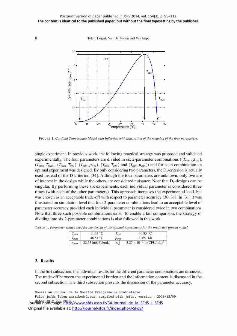
is 256, the minimum number is 118. The 6 combinations are computed in 1002 seconds. Theresulting Pareto fronts for each of the parameter combinations are displayed in Figure 2. Note thatthe values for the information content are normalized. The obtained Pareto fronts clearly indicatenon-convex feasible regions. Hence, the choice for NNC is justified. These Pareto fronts allow theexperimenter to select a specific experiment with a given amount of work. Based on the Paretofront he or she then knows the expected information amount of the experiment.

0 0.5 10

10

20

30

40

Mea

sure

men

t Tim

e (h

)

Ds,crit Tmax, µopt

0 0.5 10

10

20

30

40

Mea

sure

men

t Tim

e (h

)

Ds,crit Tmax, Tmin

0 0.5 10

10

20

30

40

Mea

sure

men

t Tim

e (h

)

Ds,crit Tmax, Topt

0 0.5 10

10

20

30

40

Mea

sure

men

t Tim

e (h

)

Ds,crit Tmin, µopt

0 0.5 10

10

20

30

40

Mea

sure

men

t Tim

e (h

)

Ds,crit Tmin, Topt

0 0.5 10

10

20

30

40

Mea

sure

men

t Tim

e (h

)

Ds,crit Topt, µopt

FIGURE 2. Pareto fronts for the six different criteria in relation to measurement time. The plus and circle indicate theindividual optima of the two considered objectives, respectively.

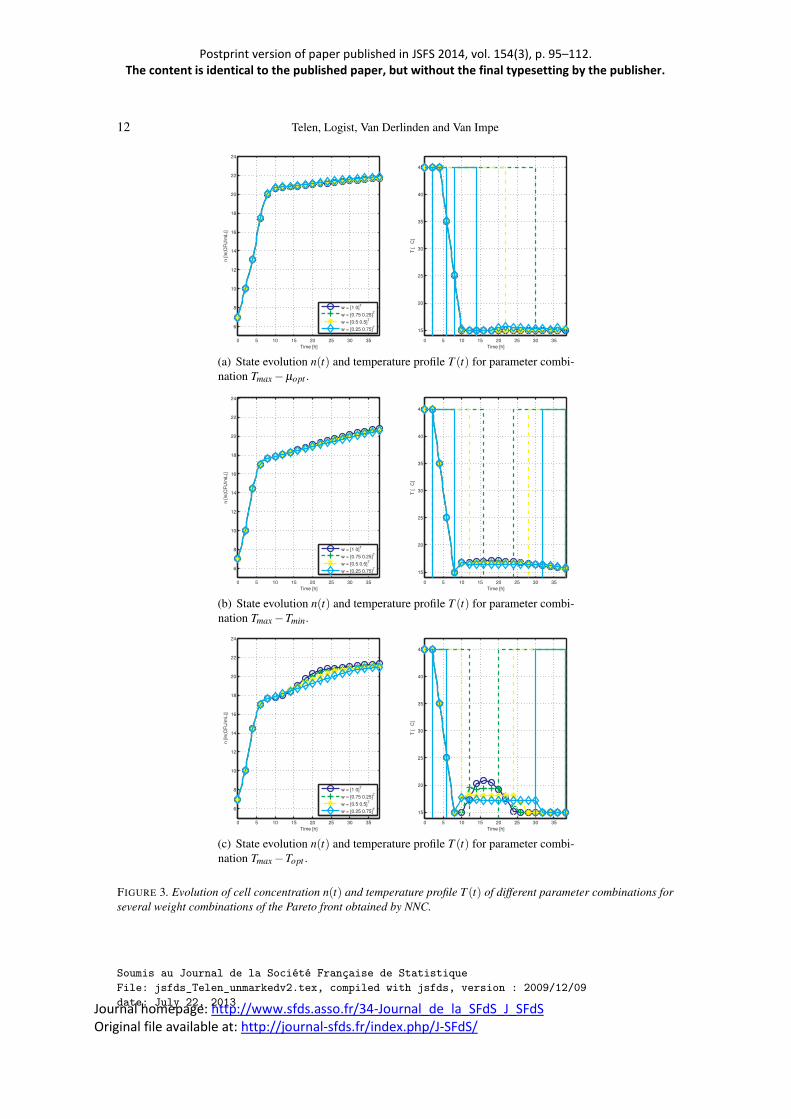
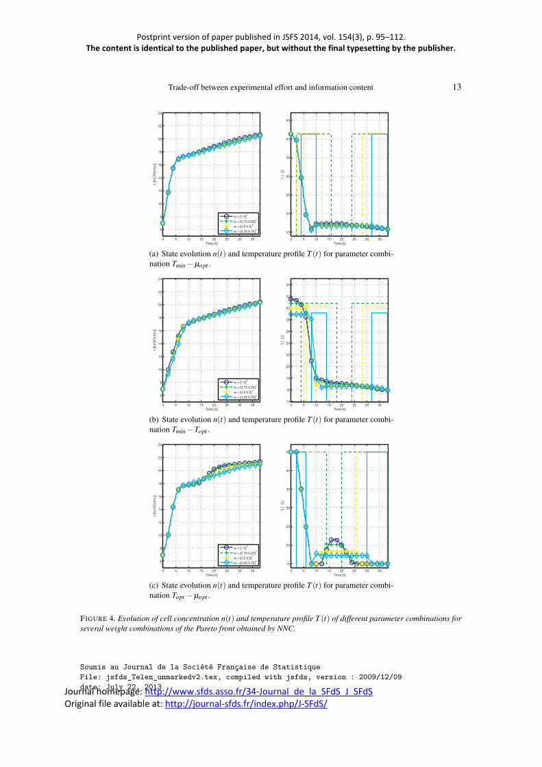
The decision when to measure influences the designed experiment. This is illustrated in Figures3 and 4. In this paragraph w, is used to indicate which multi-objective point of the utopia planeis considered. The utopia plane is the line/plane connecting the two individual objectives. Theweights, w indicate how this line is discretized in the NNC. The case with w = [1 0]T correspondsto measuring at each of the multiple shooting nodes during the experiment, so every two hours





and a maximum total of 20 samples per experiment. Other weight combinations have a reducedworkload. The lowest workload combination taken into consideration relates to weight combi-nation w = [0.25 0.75]. In the cases with a reduced workload, the experimenter is expected tosample continuously in the time horizons indicated by the rectangles in the temperature profiles ofFigures 3 and 4. The total amount of hours denoted by the integral over the intervals indicated bythe rectangles constitutes the measurement time. These coincide again with the 2-hourly multipleshooting nodes and a possible change in control action.

For the three combinations where Tmax is involved, the temperature profile starts at the max-imal allowed temperature of 45◦C. For these experiments, the decreasing part of the temperatureprofile is an interesting part for optimizing the information content. So, if only a few samplesare taken, it is advisable to do it in this part of the experiment. Note that the temperature pro-file changes in view of when samples are taken. This is shown for the parameter combinationTmax−Topt .

When Tmin is combined with Topt or µopt , the temperature profile does not start at the maxi-mal value. There also seems to be a more gentle decrease in the lower temperature region of theexperiment compared with the profiles where Tmax is present.

Combining Topt−µopt results again in a temperature profile that starts at the maximum allowedtemperature value. Note again the change of the obtained temperature profile when reducing theamount of samples that are taken.

A general observation is that all parameter combinations except Tmax− µopt have some mea-surements taken at the end of the experiment. Also the sharp decrease in temperature present in allprofiles generates information. Biologically, this corresponds to the fast growing phase of the cell,as illustrated in the corresponding cell concentration profiles (see Figure 3 and 4). Based on theseobservations, one can conclude that it is important to sample at the start (i) of the experiment,(ii) during a period of decreasing temperature, and at the end (iii) of the experiment. In previouswork, this was done from practical point of view (need of night rest) [31], but is now validatedwith these results.





0 5 10 15 20 25 30 35

6

8

10

12

14

16

18

20

22

24

Time [h]

n [ln

(CF

U/m

L)]

w = [1 0]T

w = [0.75 0.25]T

w = [0.5 0.5]T

w = [0.25 0.75]T

0 5 10 15 20 25 30 35

15

20

25

30

35

40

45

Time [h]

T [

°C

]

(a) State evolution n(t) and temperature profile T (t) for parameter combi-nation Tmax−µopt .

0 5 10 15 20 25 30 35

6

8

10

12

14

16

18

20

22

24

Time [h]

n [ln

(CF

U/m

L)]

w = [1 0]T

w = [0.75 0.25]T

w = [0.5 0.5]T

w = [0.25 0.75]T

0 5 10 15 20 25 30 35

15

20

25

30

35

40

45

Time [h]

T [

°C

]

(b) State evolution n(t) and temperature profile T (t) for parameter combi-nation Tmax−Tmin.

0 5 10 15 20 25 30 35

6

8

10

12

14

16

18

20

22

24

Time [h]

n [ln

(CF

U/m

L)]

w = [1 0]T

w = [0.75 0.25]T

w = [0.5 0.5]T

w = [0.25 0.75]T

0 5 10 15 20 25 30 35

15

20

25

30

35

40

45

Time [h]

T [

°C

]

(c) State evolution n(t) and temperature profile T (t) for parameter combi-nation Tmax−Topt .

FIGURE 3. Evolution of cell concentration n(t) and temperature profile T (t) of different parameter combinations forseveral weight combinations of the Pareto front obtained by NNC.





0 5 10 15 20 25 30 35

6

8

10

12

14

16

18

20

22

24

Time [h]

n [ln

(CF

U/m

L)]

w = [1 0]T

w = [0.75 0.25]T

w = [0.5 0.5]T

w = [0.25 0.75]T

0 5 10 15 20 25 30 35

15

20

25

30

35

40

45

Time [h]

T [

°C

]

(a) State evolution n(t) and temperature profile T (t) for parameter combi-nation Tmin−µopt .

0 5 10 15 20 25 30 35

6

8

10

12

14

16

18

20

22

24

Time [h]

n [ln

(CF

U/m

L)]

w = [1 0]T

w = [0.75 0.25]T

w = [0.5 0.5]T

w = [0.25 0.75]T

0 5 10 15 20 25 30 3514

16

18

20

22

24

26

28

30

32

34

Time [h]

T [

°C

]

(b) State evolution n(t) and temperature profile T (t) for parameter combi-nation Tmin−Topt .

0 5 10 15 20 25 30 35

6

8

10

12

14

16

18

20

22

24

Time [h]

n [ln

(CF

U/m

L)]

w = [1 0]T

w = [0.75 0.25]T

w = [0.5 0.5]T

w = [0.25 0.75]T

0 5 10 15 20 25 30 35

15

20

25

30

35

40

45

Time [h]

T [

°C

]

(c) State evolution n(t) and temperature profile T (t) for parameter combi-nation Topt −µopt .

FIGURE 4. Evolution of cell concentration n(t) and temperature profile T (t) of different parameter combinations forseveral weight combinations of the Pareto front obtained by NNC.





3.3. Assessing parameter accuracy when reducing number of samples

The obtained parameter values and the corresponding confidence regions are presented in Tables3, 4, 5 and 6. In each table, the results are grouped according to the number of measurements inthe experiments.

Parameters are estimated using a least squares objective function. Multiple shooting is em-ployed, where the shooting nodes coincide with the in silico measurements. The bounds on theparameters are:

1.5≤ µopt ≤ 4.5 (21)

6≤ Tmin ≤ 13 (22)

37≤ Topt ≤ 42 (23)

44≤ Tmax ≤ 50. (24)

The initial parameter values passed to the optimization routine are the middle values of theabove intervals. Two different approaches for computing the parameter variance are compared.One of the main possible drawbacks of the Fisher information matrix is that it can lead to anunderestimation of the confidence bounds [1]. This means that the confidence regions obtainedby the Fisher information matrix are smaller than those obtained by other approaches [12, 27].In this work, a Monte-Carlo simulation is performed to check whether this is also the case forthe CTMI. In the first approach, the model parameters are identified, and their uncertainty iscomputed using the obtained FIM. The second approach uses 500 Monte-Carlo noise realizations,each time re-estimating the parameters. The 500 individual estimates are used to construct theempirical 95% confidence region. Their average value is taken as the final parameter estimate.

The results show that the original parameters are each time located inside the obtained con-fidence region. As can be expected, the parameter confidence intervals become broader when thenumber of measurement points are decreased (and thus the workload reduced). This holds forboth the Fisher information approach and the Monte-Carlo approach. When only 45 samples aretaken compared to the 120 in the nominal case, the confidence interval, on average doubles insize.

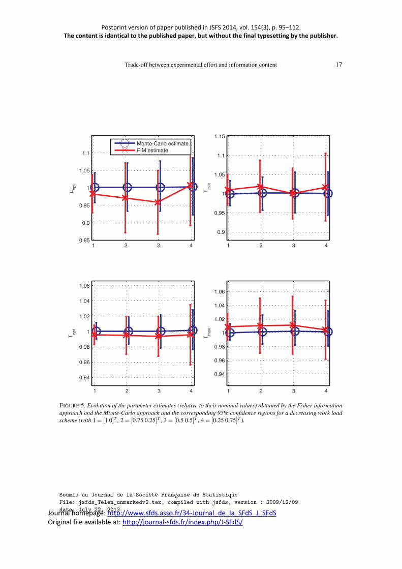
From the simulation results shown in Tables 3 to 6, one infers that the size of the confidenceintervals of the FIM and MC approaches is approximately equal. In Figure 5, the evolution of theparameter estimates and the confidence bounds for both approaches are displayed. This figureillustrates that there are only three cases where the 95% confidence bound given by the asymptoticnormal distribution of the least squares estimator is smaller than the Monte-Carlo estimate of the95% bound. Note, however, that in all cases the total width of the confidence region obtained bythe Fisher information is broader than the one obtained by the Monte-Carlo simulation. Fromthese observations, it can be inferred that the Fisher information matrix can be used to get a robustestimate of the real confidence bounds of the parameter estimates for the current case study.

An additional observation is the fact that the confidence regions for Topt and Tmax exhibit a





non-symmetrical confidence region in the Monte-Carlo simulations. The empirically obtaineddistributions have been tested for normality using the Kolmogorov-Smirnov test. The hypothesisthat Topt is normal, could not be rejected on a 5% discrimination level for all workload cases.For Tmax this hypothesis can be rejected using the same test with the same discrimination level.Note, that the Fisher information matrix yields a conservative bound for Tmax, even in view ofthe non-normal distribution of Tmax. This clearly illustrates that the uncertainty estimation by theFisher information matrix can be inaccurate and too conservative in this case study. In this casestudy, the uncertainty was too conservative. Therefore, a careful assessment of the uncertaintythrough other means than the Fisher information matrix is advisable if computationally feasible.Furthermore, if the assumption that the parameters are normal, is rejected, this means that thesample size is too small and that asymptotic normality is not reached.





TABLE 3. Parameter values and confidence regions for 120 samples in the six experiments.

Parameter FIM approach (95% CI) Monte-Carlo approach (95% CI)µopt 2.357 (±0.1299) 2.399 (−0.1042 +0.1030)Tmin 11.44 (±0.4571) 11.32 (−0.3436 +0.3876)Topt 40.68 (±0.5203) 40.86 (−0.4108 +0.4679)Tmax 46.94 (±0.8874) 46.55 (−0.5018 +0.5995)











1 2 3 40.85

0.9

0.95

1

1.05

1.1

µopt

Monte-Carlo estimate

FIM estimate

1 2 3 4

0.9

0.95

1

1.05

1.1

1.15

Tm

in

1 2 3 4

0.94

0.96

0.98

1

1.02

1.04

1.06

Topt

1 2 3 4

0.94

0.96

0.98

1

1.02

1.04

1.06

Tm

ax

FIGURE 5. Evolution of the parameter estimates (relative to their nominal values) obtained by the Fisher informationapproach and the Monte-Carlo approach and the corresponding 95% confidence regions for a decreasing work loadscheme (with 1 = [1 0]T , 2 = [0.75 0.25]T , 3 = [0.5 0.5]T , 4 = [0.25 0.75]T ).





4. Conclusion

In this work, a practical procedure is proposed to systematically evaluate trade-offs between infor-mation content and experimental effort in the design of dynamic experiments for calibrating theCardinal Temperature Model with Inflection. In the employed procedure, advanced multi-objectivedynamic optimization approaches are exploited. The considered objectives were parameter accu-racy on the one hand, and the total time reserved for measuring on the other. With respect to thelatter objective, the determination of optimal measurement/sampling schemes specifying whento measure is added as a degree of freedom. The use of advanced multi-objective optimizationallowed the experimenter to generate the set of Pareto optimal solutions. This set enables theexperimenter to obtain an overview of all the possible trade-offs. The accuracy of the designed ex-periments with reduced workload is assessed in a simulation study, because one known drawbackof the Fisher information matrix approach is that, for models non-linear in the parameters, it cangive a possibly inaccurate estimate of the confidence intervals. Hence, the validity of the Fisherinformation matrix approach is checked by performing a Monte-Carlo simulation.

Acknowledgements

Work supported in part by Projects, OT/10/035, PFV/10/002 OPTEC (Centre-of-ExcellenceOptimisation in Engineering), KP/09/005 SCORES4CHEM knowledge platform of the KULeuven, the Flemish government: G.0930.13 and FWO-1518913N and the Belgian FederalScience Policy Office: IAP PVII/19. Dries Telen has a Ph.D grant of the Agency for the Promotionof Innovation through Science and Technology in Flanders (IWT-Vlaanderen). Jan Van Impe holdsthe chair Safety Engineering sponsored by the Belgian chemistry and life sciences federationessenscia. The authors thank Geert Gins for the thorough proofreading of the final paper.

References

[1] E. Balsa-Canto, A.A. Alonso, and Banga J.R. Computing optimal dynamic experiments for model calibration inpredictive microbiology. Journal of Food Process Engineering, 31:186–206, 2007.

[2] J. Baranyi and T.A. Roberts. A dynamic approach to predicting bacterial growth in food. International Journalof Food Microbiology, 23:277–294, 1994.

[3] L.T. Biegler. Solution of dynamic optimization problems by successive quadratic programming and orthogonalcollocation. Computers and Chemical Engineering, 8:243–248, 1984.

[4] L.T. Biegler. An overview of simultaneous strategies for dynamic optimization. Chemical Engineering andProcessing: Process Intensification, 46:1043–1053, 2007.

[5] L.T. Biegler. Nonlinear Programming: Concepts, Algorithms and Applications to Chemical Engineering. SIAM,2010.

[6] H.G. Bock and K.J. Plitt. A multiple shooting algorithm for direct solution of optimal control problems. InProceedings of the 9th IFAC world congress, Budapest. Pergamon Press, 1984.

[7] I. Das and J.E. Dennis. A closer look at drawbacks of minimizing weighted sums of objectives for Pareto setgeneration in multicriteria optimization problems. Structural Optimization, 14:63–69, 1997.

[8] I. Das and J.E. Dennis. Normal-Boundary Intersection: A new method for generating the Pareto surface innonlinear multicriteria optimization problems. SIAM Journal on Optimization, 8:631–657, 1998.

[9] V.V. Fedorov. Optimal design with bounded density: optimization algorithms of the exchange type. Journal ofStatistical Planning and Inference, 22:1–13, 1989.

[10] G. Franceschini and S. Macchietto. Model-based design of experiments for parameter precision: State of the art.Chemical Engineering Science, 63:4846–4872, 2008.





[11] Y.Y. Haimes, L.S. Lasdon, and D.A. Wismer. On a bicriterion formulation of the problems of integrated systemidentification and system optimization. IEEE Transactions on Systems, Man, and Cybernetics, SMC-1:296–297,1971.

[12] T. Heine, M. Kawohl, and R. King. Derivative-free optimal experimental design. Chemical Engineering Science,63:4873–4880, 2008.

[13] B. Houska, H.J. Ferreau, and M. Diehl. ACADO Toolkit - an open-source framework for automatic control anddynamic optimization. Optimal Control Applications and Methods, 32:298–312, 2011.

[14] D.B. Leineweber, I. Bauer, H.G. Bock, and J.P. Schlöder. An efficient multiple shooting based reduced SQPstrategy for large-scale dynamic process optimization. Part I: theoretical aspects. Computers and ChemicalEngineering, 27:157–166, 2003.

[15] L. Ljung. System Identification: Theory for the User. Prentice Hall, 1999.[16] F. Logist, B. Houska, M. Diehl, and J. Van Impe. Fast pareto set generation for nonlinear optimal control

problems with multiple objectives. Structural and Multidisciplinary Optimization, 42:591–603, 2010.[17] F. Logist, D. Telen, B. Houska, M. Diehl, and J. Van Impe. Multi-objective optimal control of dynamic

bioprocesses using ACADO toolkit. Bioprocess and Biosystems Engineering, 36:151–164, 2013.[18] F. Logist, M. Vallerio, B. Houska, M. Diehl, and J. Van Impe. Multi-objective optimal control of chemical

processes using ACADO toolkit. Computers and Chemical Engineering, 37:191–199, 2012.[19] F. Logist and J. Van Impe. Novel insights for multi-objective optimisation in engineering using normal boundary

intersection and (enhanced) normalised normal constraint. Structural and Multidisciplinary Optimization,45:417–431, 2012.

[20] A. Messac, A. Ismail-Yahaya, and C.A. Mattson. The normalized normal constraint method for generating thePareto frontier. Structural & Multidisciplinary Optimization, 25:86–98, 2003.

[21] K. Miettinen. Nonlinear multiobjective optimization. Kluwer Academic Publishers, Boston, 1999.[22] L. Pontryagin, V. Boltyanskiy, R. Gamkrelidze, and Y. Mishchenko. The mathematical theory of optimal

processes. Wiley - Interscience, New York, 1962.[23] F. Pukelsheim. Optimal design of Experiments. John Wiley & Sons, Inc., New York, 1993.[24] L. Rosso, J.R. Lobry, and J.P. Flandrois. An unexpected correlation between cardinal temperatures of microbial

growth highlighted by a new model. Journal of Theoretical Biology, 162:447–463, 1993.[25] S. Sager. Sampling decisions in optimum experimental design in the light of Pontryagin’s maximum principle.

SIAM Journal on Control and Optimization, 2012. (submitted).[26] R.W.H. Sargent and G.R. Sullivan. The development of an efficient optimal control package. In J. Stoer,

editor, Proceedings of the 8th IFIP Conference on Optimization Techniques, pages 158–168, Heidelberg, 1978.Springer-Verlag.

[27] R. Schenkendorf, A. Kremling, and M. Mangold. Optimal experiment design with the sigma point method.Systems Biology, 3:10–23, 2009.

[28] L. Sonneborn and F. Van Vleck. The bang-bang principle for linear control systems. J. SIAM Control, Ser. A,2:151–159, 1965.

[29] D. Telen, F. Logist, E. Vanderlinden, and J. Van Impe. Optimal experiment design for dynamic bioprocesses: amulti-objective approach. Chemical Engineering Science, 78:82–97, 2012.

[30] E. Van Derlinden. Quantifying microbial dynamics as a function of temperature: towards an optimal trade-offbetween biological and model complexity. PhD thesis, 2009.

[31] E. Van Derlinden, K. Bernaerts, and J. Van Impe. Simultaneous versus sequential optimal experiment designfor the identification of multi-parameter microbial growth kinetics as a function of temperature. Journal ofTheoretical Biology, 264:347–355, 2010.

[32] V.S. Vassiliadis, R.W.H. Sargent, and C.C. Pantelides. Solution of a class of multistage dynamic optimizationproblems. 1. Problems without path constraints. Industrial and Engineering Chemistry Research, 33:2111–2122,1994.

[33] V.S. Vassiliadis, R.W.H. Sargent, and C.C. Pantelides. Solution of a class of multistage dynamic optimizationproblems. 2. Problems with path constraints. Industrial and Engineering Chemistry Research, 33:2123–2133,1994.

[34] E. Walter and L. Pronzato. Identification of Parametric Models from Experimental Data. Springer, Paris, 1997.


Documents

The content is identical to the content of the published ... · d’expériences optimaux pour la calibration d’un modèle de la microbiologie prédictive Dries Telen 1, Filip Logist